MAD-TH-14-03

IPMU-14-0094

Boundaries and Defects of ${\cal N}=4$ SYM with 4 Supercharges

Part I: Boundary/Junction Conditions

Akikazu Hashimoto^a, Peter Ouyang^b, and Masahito Yamazaki^c,d

^a Department of Physics, University of Wisconsin, Madison, WI 53706, USA

^b Department of Physics, Purdue University, West Lafayette, IN 47907, USA

^c Institute for Advanced Study, Princeton, NJ 08540, USA

^d Kavli IPMU (WPI), University of Tokyo, Kashiwa, Chiba 277-8583, Japan

We consider ${\cal N}=4$ supersymmetric Yang Mills theory on a space with supersymmetry preserving boundary conditions. The boundaries preserving half of the 16 supercharges were analyzed and classified in an earlier work by Gaiotto and Witten. We extend that analysis to the case with fewer supersymmetries, concentrating mainly on the case preserving one quarter. We develop tools necessary to explicitly construct boundary conditions which can be viewed as taking the zero slope limit of a system of D3 branes intersecting and ending on a collection of NS5 and D5 branes oriented to preserve the appropriate number of supersymmetries. We analyze how these boundary conditions constrain the bulk degrees of freedom and enumerate the unconstrained degrees of freedom from the boundary/defect field theory point of view. The key ingredients used in the analysis are a generalized version of Nahm’s equations and the explicit boundary/interface conditions for the NS5-like and D5-like impurities and boundaries, which we construct and describe in detail. Some bulk degrees of freedom suggested by the naive brane diagram considerations are lifted.

1 Introduction

Impurities, defects, and boundaries are important objects in the study of field theories. The dynamics of the field theory itself can generate defects nonperturbatively, and the existence or nonexistence of certain defect solutions can serve as a probe for the phase structure of the theory. It can also be interesting to study boundary conditions abstractly, in terms of conditions imposed on the fields. In the presence of boundaries and impurities, one often encounters edge effects and localized degrees of freedom which can give rise to interesting physics.

The generic study of defects and boundaries is an enormous subject, which touches on the physics of essentially every field theory. To sharpen this study, it is useful to restrict to supersymmetric field theories and boundaries which preserve some fraction of the bulk supersymmetry. For example, by studying the supersymmetric boundaries of two dimensional superconformal field theory, one uncovers the existence of D-branes and other worldsheet boundary states.

Another natural class of systems one can consider is the set of boundaries preserving half of the supersymmetries of the maximally supersymmetric Yang-Mills (SYM) theory with gauge group $G$ in 3+1 dimensions. These boundaries were studied extensively by Gaiotto and Witten (GW) [1, 2]. Their treatment begins with a study of the BPS field configurations on a half-space with translation invariance broken in one direction; the relevant Bogomolny-type equations are the Nahm equations [3]. Using intuition from string theory realizations [4], GW formulated a low-energy classification of the boundary conditions in terms of a triple $(\rho,H,\mathfrak{B})$[1, 2]. Here $\rho$ is an embedding of $\mathfrak{sl}(2)$ into $\mathfrak{g}$ (the Lie algebra of $G$) representing the Nahm pole, gauge group $G$ is broken to a subgroup $H$ of the commutant of $\rho$ at the boundary, and $\mathfrak{B}$ is a 3$d$ $\mathcal{N}=4$ boundary theory with global symmetry $H$. Moreover, they gave a recipe for relating the action of S-duality on a given 1/2 BPS boundary condition to the action of mirror symmetry on a related 3$d$ theory, which they constructed by coupling a given boundary condition to a 3$d$ theory called $T[SU(N)]$ [2].

Our work initially stemmed out of a rather innocent inquiry: how does the structure of boundaries and their classification generalize if they preserve less than half of the original supersymmetry? Generally, we expect richer physics when the amount of supersymmetry is reduced. Would we discover an object, generalizing the NS5-branes or the D5-branes, on which a D3 can end and preserve less than half of the supersymmetries? Is there a simple generalization to the triple $(\rho,H,\mathfrak{B})$ that one can formulate to generalize the GW classification?

We have encountered a number of subtleties in answering these questions. Below, we will review the formalism of GW, and show that attempts to construct an elementary 1/4 BPS object analogous to an NS5 brane or a D5 brane do not lead to anything new. We can construct boundaries and defects preserving less than half of the supersymmetries by including 5-branes oriented in such a way that each of the 5-branes break different components of the supersymmetries. We can attempt to classify different configurations of stacks of NS5 and D5 branes arranged to preserve some fraction of supersymmetries. Such a classification, however, will be more complicated than the results in the 1/2 BPS case. The main reason is the fact that in the 1/2 BPS analysis, changing the positions of the 5-branes does not change the low energy physics. This allowed GW to define a canonical ordering of the 5-branes, and this feature was used to dramatically reduce the set of possible boundaries. In the cases with less than 8 supersymmetries, however, the changes in the ordering of the 5-branes can, in general, change the low energy physics. This does not necessarily imply that a classification for these boundaries is impossible, but it does imply that such a classification will be far more intricate than when 8 supersymmetries are preserved.

Even if the classification scheme for 1/2 BPS boundaries does not generalize easily to the case of 1/4 BPS, it is interesting to explore the rich dynamics of boundaries with less supersymmetries. In this paper, we will construct several examples of boundaries preserving 1/4 of the supersymmetries of ${\cal N}=4$ supersymmetric Yang-Mills theory by combining a collection of NS5 and D5-branes. These structures possess localized as well as delocalized degrees of freedom, which in a loose sense could be considered the moduli space of the boundary. Through explicit analysis of the Lagrangian of this system in the classical limit, we map out these deformations, which have a natural Kähler structure as a result of having 4 supercharges.

These boundary conditions can then be used as building blocks for engineering ${\cal N}=2$ field theories in 2+1 dimensions, for instance, by considering the 4$d$ $\mathcal{N}=4$ theory on an interval with boundary conditions at both ends. On the interval, there are no issues with the delocalized modes and the notion of a moduli space is well defined. Strictly speaking, our analysis is limited to classical dynamics. However, for ${\cal N}=4$ theory in 3+1 dimensions on an interval, we can also analyze the moduli space of the S-dual configuration in the classical limit. Depending on the pattern of gauge symmetry breaking, which can be mapped nontrivially by duality, we can gain access to some quantum corrected features of the model by doing classical computations in the S-dual.

In addition, there are non-renormalization theorems for systems with ${\cal N}=2$ supersymmetries in 2+1 dimensions [5]. We expect superpotentials to be protected from corrections at the perturbative level. However, superpotential terms can be generated dynamically at the non-perturbative level through instantons as was shown in [6]. On the other hand, we expect the instanton corrections to be absent in branches where all of the gauge symmetries are spontaneously broken. Generally, the information contained in the $D$-terms (which encodes the metric data of the moduli space through the Kähler potential) are subjected to corrections, but there are situations where even the Kähler potential is protected from quantum corrections [7, 8].

One interesting application of our program is to map out (as much as possible) the fully quantum corrected moduli space of systems using the data available from the combination of S-duality and the assortment of non-renormalization theorems. In this paper, we will begin this program by performing a detailed analysis of boundaries which preserve 1/4 of the supersymmetry. The application to ${\cal N}=2$ theories in 2+1 dimensions by placing the $\mathcal{N}=4$ theory on a finite interval with boundary conditions on both ends of the interval will appear in a separate paper [9]. We will assess the power of this approach and attempt to extract some general lessons by working out numerous concrete examples with varying degrees of complexity. Although we mostly study the case where $1/4$ of the supersymmetries are preserved, some of our methods extend easily to the cases with $3/8$ or $1/8$ of the supersymmetries being preserved.

2 Basic Construction of Boundaries in 4$d$ ${\cal N}=4$ SYM

In this section, we describe the construction of supersymmetric boundary conditions in ${\cal N}=4$ SYM in 3+1 dimensions. We will begin by reviewing the construction of boundaries preserving half of the supersymmetries of the bulk theory (section 2.1), following the treatment of [1], whose conventions we adopt. We then describe the generalization to the case preserving a quarter of the supersymmetries (section 2.2). We also comment on more general composite boundary conditions (section 2.3) and on the classification of 1/4 BPS boundary conditions (section 2.4).

Before going into the details, we will make a few general remarks about our analysis:

1. Throughout this paper, we distinguish between “bulk” properties which refer to the 3+1-dimensional theory and “boundary” or “interface” properties which refer to 2+1-dimensional defects embedded in the 3+1-dimensional bulk.

2. In this section, we assume that the boundaries themselves do not carry any dynamical degrees of freedom of their own. As we will see, this assumption often does not hold in practical applications, and we will relax this assumption later in section 3.

3. We will not make use of the conformal symmetry (or its fermionic counterpart) of the the $\mathcal{N}=4$ SYM theory in the discussion of the boundary conditions. Our boundary conditions in general break conformal symmetry, which is recovered only in the IR limit. This is in contrast with the discussion of boundary conformal field theories, which relies crucially on conformal symmetry.

4. While our discussion in this paper deals with 4$d$ $\mathcal{N}=4$ SYM, the approach we follow is rather general. It would be interesting to apply the same methods to supersymmetric boundary conditions for other theories in various dimensions; for example, 1/2 BPS boundary conditions of 4$d$ $\mathcal{N}=2$ theories [10] should also give rise to 3$d$ $\mathcal{N}=2$ theories associated with 3-manifolds [11, 12].

Let us first recall the basics of 4$d$ $\mathcal{N}=4$ theory, and set up some notation. The ${\cal N}=4$ SYM in 3+1 dimensions can be efficiently obtained from ${\cal N}=1$ SYM in 9+1 dimensions. Our convention is that the 10$d$ metric $g_{IJ}$ ($I,J=0,\ldots,9$) has signature $(-,+,\cdots+)$ and the Clifford-Dirac algebra is $\{\Gamma_{I},\Gamma_{J}\}=2g_{IJ}$. The 10$d$ chirality operator is $\bar{\Gamma}\equiv\Gamma_{0}\Gamma_{1}\cdots\Gamma_{9}$. The 10$d$ SYM action is

$$I={1\over g_{\rm YM4}^{2}}\int d^{10}x\,{\rm Tr}\left({1\over 2}F_{IJ}F^{IJ}-i\bar{\Psi}\Gamma^{I}D_{I}\Psi\right),$$ (2.1)

where $A_{I}$ is a gauge field whose field strength we defined to be $F_{IJ}\equiv\partial_{I}A_{J}-\partial_{J}A_{I}{-}[A_{I},A_{J}]$, and $\Psi$ is a Majorana-Weyl fermion satisfying $\Psi=\bar{\Gamma}\Psi$. We use the convention that the bosonic fields are anti-hermitian, so the field strength $F_{IJ}$ is defined without a factor of $i$ in front of the commutator. The fields transform under supersymmetry as

$$\delta A_{I} = i\bar{\varepsilon}\,\Gamma_{I}\Psi\ ,$$ (2.2)

$$\delta\Psi = {1\over 2}\Gamma^{IJ}F_{IJ}\varepsilon\ .$$ (2.3)

The supersymmetry generator $\varepsilon$ is also Majorana-Weyl and satisfies $\varepsilon=\bar{\Gamma}\varepsilon$. The supercurrent associated with these transformations is

$$J^{I}={1\over 2}{\rm Tr}\,\Gamma^{JK}F_{JK}\Gamma^{I}\Psi.$$ (2.4)

The 3+1-dimensional ${\cal N}=4$ SYM theory can now be obtained by dimensional reduction of the 10$d$ theory, with the ansatz that the fields depend only on $x^{0},\cdots,x^{3}$. It is conventional to re-label the components of the gauge fields as $A_{3+i}=\Phi_{i}$ for $i=1\ldots 6$; these transform as scalars under the $SO(3,1)$ Lorentz symmetry.

We will take the boundary to be flat, extended in $x_{0}$, $x_{1}$, and $x_{2}$ coordinates, and localized at some fixed $y\equiv x_{3}$ coordinate. This breaks translation invariance in the $y$ direction.

The condition that the boundary preserves supersymmetry is that the flux of the supercurrent through the boundary vanishes, or in other words

$$J^{3}\big{|}={\rm Tr}\,\bar{\varepsilon}\,\Gamma^{IJ}F_{IJ}\Gamma_{3}\Psi\big{|}=0\ ,$$ (2.5)

where the symbol $\big{|}$ means that the equation holds at the boundary. Since the 3+1 dimensional Lorentz is broken by the presence of the boundary, we cannot impose (2.5) for all the sixteen supercharges; to preserve half (a quarter) of the supersymmetry, we impose (2.5) for 8 (4) of the 16 components of $\varepsilon$.

The boundary condition eliminates half of the degrees of the freedom at the boundary. For bosons, we could choose Dirichlet or Neumann, or more generally mixed boundary conditions. For the fermions, the boundary condition sets half of the components of $\Psi$ to some fixed values (using the Dirac equation, one sees that Dirichlet boundary conditions for half the fermionic degrees of freedom imposes Neumann boundary conditions for the other half.) We then need to see which of these boundary conditions are consistent with (2.5).

While we are mainly interested in boundary conditions in this paper, it is also useful to consider the BPS condition in the bulk. The bulk equations are especially important if we wish to construct complicated boundary conditions by starting with several boundary/junction conditions separated by the bulk theory on the interval, and then take the limit where the defects collide, as illustrated in figure 1. This limit is equivalent to the taking the IR limit of the composite boundary. These composite boundary conditions contain the bulk degrees of freedom on the interval, which are crucial for the analysis of the moduli space of the boundary condition. The same remark applies to the analysis of the 3$d$ field theory discussed in our second paper [9].

The bulk BPS equation is given by

$$\,\delta\bar{\Psi}=\bar{\varepsilon}\,\Gamma^{IJ}F_{IJ}=0\ ,$$ (2.6)

where the right hand side refers to $\varepsilon$ but not to $\Psi$.

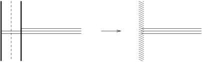
Figure 1: By collapsing the boundary conditions we can construct more complicated boundary conditions. For this analysis it is necessary to keep track of the bulk degrees of freedom between the two defects, which is constrained by (2.6).

Clearly, the bulk BPS condition (2.6) is stronger than the boundary BPS condition for fermions (2.5), in that the former restricted to the boundary implies the latter. This is not necessarily the case for scalars. In some cases (for example for the Neumann boundary condition for the scalar field) the actual boundary condition is contained in the supersymmetry condition (2.5); in other cases (for example for the Dirichlet boundary condition) we have to impose the boundary condition separately. We will see concrete examples momentarily.

2.1 Boundaries Preserving Half of the Supersymmetries

Let us now consider the construction of boundaries preserving half of the 16 supersymmetries.

To proceed further in analyzing these equations, it is useful to parametrize $\varepsilon$ and $\Psi$ to maximally reflect the symmetries of the problem. Here, the key feature is that the symmetry of the bulk boundary system is equivalent to the symmetry of ${\cal N}=4$ supersymmetry in 2+1 dimensions, whose $R$ symmetry is $SO(4)\simeq SO(3)_{X}\times SO(3)_{Y}$. As the notation suggests, we can identify these $SO(3)$’s as acting on two sets of three transverse scalars which we label

$$(X_{1},X_{2},X_{3})\equiv(\Phi_{1},\Phi_{2},\Phi_{3})\ ,\qquad(Y_{1},Y_{2},Y_{3})\equiv(\Phi_{4},\Phi_{5},\Phi_{6})\ .$$ (2.7)

Let us define

$$\begin{split}B_{0}&\equiv\Gamma_{456789}\ ,\cr B_{1}&\equiv\Gamma_{3456}\ ,\cr B_{2}&\equiv\Gamma_{3789}\ .\end{split}$$ (2.8)

These form an $SL(2,\mathbb{R})$ algebra. In the representation of appendix A, these can be represented by

$$B_{0} = \left(\begin{array}[]{cc}0&1\\ -1&0\end{array}\right)\ ,$$ (2.11)

$$B_{1} = \left(\begin{array}[]{cc}0&1\\ 1&0\end{array}\right)\ ,$$ (2.14)

$$B_{2} = \left(\begin{array}[]{cc}1&0\\ 0&-1\end{array}\right)\ .$$ (2.17)

Moreover these matrices commute with the $SO(3)_{X}\times SO(3)_{Y}$ symmetry, as well as the (2+1)-dimensional Lorentz symmetry $SO(2,1)$. The supercharges, which are in 16 of $SO(1,9)$, can then be represented as $V_{8}\otimes V_{2}$. Here $V_{2}$ is the two dimensional space on which the representation (2.14) of $SL(2,\mathbb{R})$ acts, and $V_{8}$ is the $({\bf 2},{\bf 2},{\bf 2})$ of $SO(1,2)\times SO(3)_{X}\times SO(3)_{Y}$. Some of these details will be reviewed in the appendix A.

Armed with this amount of structure, we parametrize

$$\varepsilon=v\otimes\varepsilon_{0}\in V_{8}\otimes V_{2}\ ,$$ (2.18)

and similarly

$$\Gamma_{3}\Psi=\Psi^{\prime}\otimes\vartheta\in V_{8}\otimes V_{2}\ .$$ (2.19)

Here $\varepsilon_{0}$ and $\vartheta$ are specific, fixed 2 component vectors, and $v$ and $\Psi^{\prime}$ are arbitrary eight component vectors. The choice of $\varepsilon_{0}$ specifies which 8 out of 16 components of the supersymmetry generator $\varepsilon$ are preserved. The choice of $\vartheta$, on the other hand, specifies the components of $\Psi$ which are allowed to take arbitrary values at the boundary. Components orthogonal to $\Psi^{\prime}\otimes\vartheta$, on the other hand, must vanish at the boundary.

We can now substitute (2.18), (2.19) back into the boundary BPS condition (2.5) and the bulk BPS condition (2.6) For the boundary condition (2.5), we arrive at the following set of conditions (see appendix A for more details)

$$\bar{\varepsilon}_{0}\left(F_{\mu\nu}-\epsilon_{\mu\nu\lambda}F^{3\lambda}B_{0}\right)\,\vartheta\,\big{|} = 0\ ,$$ (2.20)

$$D_{\mu}X_{a}\,\left(\bar{\varepsilon}_{0}B_{2}\vartheta\right)\big{|} = 0\ ,$$ (2.21)

$$D_{\mu}Y_{m}\,\left(\bar{\varepsilon}_{0}B_{1}\vartheta\right)\big{|} = 0\ ,$$ (2.22)

$$[X_{a},Y_{m}]\,\left(\bar{\varepsilon}_{0}B_{0}\vartheta\right)\big{|} = 0\ ,$$ (2.23)

$$\bar{\varepsilon}_{0}\left([X_{b},X_{c}]-\epsilon_{abc}D_{3}X_{a}B_{1}\right)\vartheta\,\big{|} = 0\ ,$$ (2.24)

$$\bar{\varepsilon}_{0}\left([Y_{m},Y_{n}]-\epsilon_{mnp}D_{3}Y_{p}B_{2}\right)\vartheta\,\big{|} = 0\ .$$ (2.25)

Since we have the choice of the $\varepsilon_{0}$ and $\vartheta$ up to their overall normalization, we could in principle have a 2-parameter family of boundary conditions. It turns that only one parameter survives. Two special points in the 1-parameter space corresponds to D5-like and NS5-like boundary conditions, which we discuss in turn.

2.1.1 D5-like Boundary

Consider setting

$$\bar{\varepsilon}_{0} = \frac{1}{\sqrt{2}}(1\;\;\;1)\ ,$$ (2.26)

$$\vartheta = \frac{1}{\sqrt{2}}\left(\begin{array}[]{c}1\\ 1\end{array}\right)\ .$$ (2.29)

Then

$$\bar{\varepsilon}_{0}B_{0}\vartheta=\bar{\varepsilon}_{0}B_{2}\vartheta=0\ .$$ (2.30)

Then, the bulk BPS equation (2.6) reads

$$F_{\mu\nu} = 0\ ,$$ (2.31)

$$F_{3\lambda} = 0\ ,$$ (2.32)

$$D_{\mu}X_{a} = 0\ ,$$ (2.33)

$$D_{\mu}Y_{m} = 0\ ,$$ (2.34)

$$[X_{a},Y_{m}] = 0\ ,$$ (2.35)

$$[X_{b},X_{c}]-\epsilon_{abc}D_{3}X_{a} = 0\ ,$$ (2.36)

$$[Y_{m},Y_{n}] = 0\ ,$$ (2.37)

$$D_{3}Y_{m} = 0\ .$$ (2.38)

The most important part of this equation is the Nahm equation for the $X_{a}$:

$$D_{3}X_{a}-\frac{1}{2}\epsilon_{abc}[X_{b},X_{c}] = 0\ .$$ (2.39)

The appearance of Nahm’s equations in D-brane physics was originally noted in [13]. This equation will play crucial roles in our subsequent analysis.

The boundary BPS equations (2.5) are a slightly weaker subset of these equations:

$$F_{\mu\nu}\big{|} = 0\ ,$$ (2.40)

$$D_{\mu}Y_{m}\big{|} = 0\ ,$$ (2.41)

$$\left([X_{b},X_{c}]-\epsilon_{abc}D_{3}X_{a}\right)\big{|} = 0\ ,$$ (2.42)

$$[Y_{m},Y_{n}]\big{|} = 0\ .$$ (2.43)

The boundary conditions consistent with these are

$$\textrm{D5-like}:\quad F_{\mu\nu}\big{|}=\left(D_{3}X_{a}-\frac{1}{2}\epsilon_{abc}[X_{b},X_{c}]\right)\Big{|}=Y_{m}\big{|}=0\ .$$ (2.44)

When $[X_{a},X_{a}]\big{|}=0$, this means that we have Dirichlet boundary condition for $(A_{\mu},X_{a})$ and Neumann boundary condition for $(A_{3},Y_{m})$; in 3$d$ $\mathcal{N}=4$ language each of these makes up a 3$d$ $\mathcal{N}=4$ hypermultiplet. Note that the boundary condition for gauge fields should be imposed in a gauge invariant manner, and hence we have for example $F_{\mu\nu}\big{|}=0$, and not $A_{\mu}\big{|}=0$.

Since $X_{a}$ ($Y_{m}$) obey Neumann (Dirichlet) conditions, the boundary condition (2.44) can be interpreted as a boundary condition for the D5-brane extended along the $012456$ directions. This is the reason why the boundary condition (2.44) was called “D5-like.”

If the D3 brane extends on both sides of the D5, there will be some additional localized degrees of freedom. The boundary condition (2.44) can be recovered as a limit of this more general junction condition which we will review in section 3.

When the commutator term $[X_{b},X_{c}]$ in (2.44) is nonzero, a new structure emerges. After setting $A_{3}=0$ by a choice of gauge, the equation (2.44) becomes

$$\frac{dX_{a}}{dy}-\frac{1}{2}\epsilon_{abc}[X_{b},X_{c}] = 0\ ,$$ (2.45)

which has a singular solution of the form

$$X_{a}\sim\frac{\rho(t_{a})}{y}+\mathcal{O}(y^{0})\ ,$$ (2.46)

where we have chosen the boundary to be at $y=0$, and $t^{a}$ are three matrices satisfying the $\mathfrak{sl}(2)$ commutation relation $[t_{a},t_{b}]=-\epsilon_{abc}t_{c}$, and $\rho$ is an embedding of $\mathfrak{sl}(2)$ into the gauge group $\mathfrak{g}$ (this is the same $\rho$ as appears in introduction). This means we can impose (2.46) instead of the standard Neumann boundary condition. This $1/y$ singularity is often called a “Nahm pole” in the literature.

While the singular boundary condition with a pole might unfamiliar to some of the readers, the singularity (2.46) naturally describes the funnel of D3-branes ending on D5-branes [14, 15]. It is also the case the the singular boundary conditions of this kind are required in order for the S-duality to NS5-like boundaries to work in detail. Let us now turn to that example.

2.1.2 NS5-like Boundary

Another choice for specializing (2.20)–(2.25) is to set

$$\bar{\varepsilon}_{0} = \frac{1}{\sqrt{2}}(1\;\;\;1)\ ,$$ (2.48)

$$\vartheta = \frac{1}{\sqrt{2}}\left(\begin{array}[]{c}-1\\ 1\end{array}\right)\ ,$$ (2.51)

so that

$$\bar{\varepsilon}_{0}\vartheta=\bar{\varepsilon}_{0}B_{1}\vartheta=0\ .$$ (2.52)

Because the choice of $\varepsilon_{0}$ is the same as before, this system should preserve the same set of supersymmetries. The bulk equation (2.6) is therefore the same as before. However, because $\vartheta$ is different, the boundary condition changes. In fact, the boundary BPS condition (2.5) will now read

$$F^{3\lambda}\big{|} = 0\ ,$$ (2.53)

$$D_{\mu}X_{a}\big{|} = 0\ ,$$ (2.54)

$$[X_{a},Y_{m}]\big{|} = 0\ ,$$ (2.55)

$$D_{3}Y_{m}\big{|} = 0\ .$$ (2.56)

The boundary condition consistent with these BPS conditions are

$$\textrm{NS5-like}:F_{3\mu}\big{|}=X_{a}\big{|}=D_{3}Y_{m}\big{|}=0\ ,$$ (2.57)

which can be represented as an NS5-brane extended along the $012789$-directions.

The NS5-like boundary condition, when we exchange $456$-directions with $789$-directions, might appear to be somewhat similar to the D5-like boundary conditions, in that one of $X,Y$ obeys Dirichlet boundary conditions, and the other Neumann. However, note that we do not have the commutator $[Y_{m},Y_{n}]$ this time for the Neumann boundary condition, and hence the singular solution (2.46) is not allowed for $Y_{m}$. The generalization to the case where some number of D3 branes ends on both sides of the NS5 brane will be discussed in section 3.

2.1.3 $(p,q)$ 5-brane-like Boundary

One other possibility considered by GW in [1] can be interpreted as “$(p,q)$ 5-brane like.” Somewhat interestingly, $p/q$ does not necessarily need to be a rational number, in which case $p/q$ can still be interpreted as the $\theta$-angle of the $\mathcal{N}=4$ SYM. One can also consider various rotations of 5-branes in the 456789 coordinates. These appear to correspond, in some sense, to the exhaustive set of elementary boundaries with no explicit boundary degrees of freedom. The D5, the NS5, and the $(p,q)$ also impose conditions on the set of allowed gauge transformations at the interface, as we will illustrate in more detail below. More sophisticated boundaries are then constructed by introducing multiple sets of NS5 and D5 branes, as was described in [1, 2].

2.2 Boundaries Preserving 1/4 of the Supersymmetries

We have now accumulated enough tools to study the properties of boundaries breaking all but one quarter of supersymmetries of ${\cal N}=4$ SYM in 3+1 dimensions. The problem we want to solve is to repeat the analysis of the boundary supersymmetry condition (2.5) but with the requirement that only four of the components of $\varepsilon$ need to be nonzero.

An efficient way to do the computation is to insert a projection operator $\hat{P}$ which annihilates half the components of $\varepsilon$, and study the resulting supersymmetry condition:

$${\rm Tr}\,\bar{\varepsilon}\hat{P}\Gamma^{IJ}F_{IJ}\Gamma_{3}\Psi=0\ .$$ (2.58)

The advantage of working with the projection operators is that we can avoid explicitly writing the supersymmetry generators and work instead with the algebra of Dirac matrices. Under the decomposition $\varepsilon=v\otimes\epsilon_{0}$, we see that $\hat{P}$ must act on $v$ since $\epsilon_{0}$ has already been fixed to pick out 8 independent components. This projection operator should further break the $SO(3)_{X}\times SO(3)_{Y}$ R-symmetry. This is to be expected since the amount of supersymmetry left unbroken in the 2+1 dimensional sense is that of ${\cal N}=2$ supersymmetry, whose R-symmetry group, $SO(2)$, is much smaller. We will however consider mostly the case where there is an accidental global symmetry $SO(2)\times SO(2)$ which corresponds to orienting the NS5 and D5 branes at right angles.

Let us pause to make a comment about the notation. When discussing constructions with one quarter of supersymmetries, we use the notation

$$(X_{4},X_{5},\ldots,X_{9})\equiv(\Phi_{1},\Phi_{2},\ldots,\Phi_{6})\ .$$ (2.59)

When discussing constructions preserving one half of the supersymmetries, we will continue to use $X_{a}$ and $Y_{a}$ with the index $a$ ranging from 1 to 3. At later stages, we will also combine some of these components into complex combinations. Care has been made to make sure that this issue of notation is clear from context.

Just as we had some freedom in choosing the $\varepsilon_{0}$ and $\vartheta$, we have the freedom to chose $\hat{P}$ which in essence is the choice of which components of supersymmetry to preserve. One natural candidate we will consider is to take

$$\hat{P}=1-\Gamma_{4578}$$ (2.60)

which projects out half of the components of $v$. Note that this projection is compatible with an $SO(2)\times SO(2)$ global symmetry corresponding to rotations in the 45 and 78 planes.

For this choice of $\hat{P}$, the boundary condition (2.58) is given by

$$D_{3}X_{4}\left(\bar{\varepsilon}_{0}B_{1}\vartheta\right)-\left[X_{5},X_{6}\left(\bar{\varepsilon}_{0}\vartheta\right)-X_{9}\left(\bar{\varepsilon}_{0}B_{0}\vartheta\right)\right] = 0\ ,$$ (2.61)

$$D_{3}X_{5}\left(\bar{\varepsilon}_{0}B_{1}\vartheta\right)+\left[X_{4},X_{6}\left(\bar{\varepsilon}_{0}\vartheta\right)-X_{9}\left(\bar{\varepsilon}_{0}B_{0}\vartheta\right)\right] = 0\ ,$$ (2.62)

$$D_{3}X_{7}\left(\bar{\varepsilon}_{0}B_{2}\vartheta\right)-\left[X_{8},X_{9}\left(\bar{\varepsilon}_{0}\vartheta\right)-X_{6}\left(\bar{\varepsilon}_{0}B_{0}\vartheta\right)\right] = 0\ ,$$ (2.63)

$$D_{3}X_{8}\left(\bar{\varepsilon}_{0}B_{2}\vartheta\right)+\left[X_{7},X_{9}\left(\bar{\varepsilon}_{0}\vartheta\right)-X_{6}\left(\bar{\varepsilon}_{0}B_{0}\vartheta\right)\right] = 0$$ (2.64)

$$\bar{\varepsilon}_{0}B_{0}\vartheta\left(\left[X_{4},X_{7}\right]-\left[X_{5},X_{8}\right]\right) = 0\ ,$$ (2.65)

$$\bar{\varepsilon}_{0}B_{0}\vartheta\left(\left[X_{4},X_{8}\right]+\left[X_{5},X_{7}\right]\right) = 0\ ,$$ (2.66)

$$\bar{\varepsilon}_{0}B_{0}\vartheta\left(\left[X_{6},X_{9}\right]\right) = 0\ ,$$ (2.67)

$$D_{3}X_{6}\left(\bar{\varepsilon}_{0}B_{1}\vartheta\right)-\left[X_{4},X_{5}\right]\left(\bar{\varepsilon}_{0}\vartheta\right)+D_{3}X_{9}\left(\bar{\varepsilon}_{0}B_{2}\vartheta\right)-\left[X_{7},X_{8}\right]\left(\bar{\varepsilon}_{0}\vartheta\right) = 0\ ,$$ (2.68)

along with equations with Lorentz indices which do not play an important role for the Lorentz-invariant solutions we are interested in.

Now, let us choose

$$\bar{\varepsilon}_{0}=\frac{1}{\sqrt{2}}(1\;\;\;1)$$ (2.69)

as we did in the previous section. We can then read off the bulk equations

$$D_{3}X_{4}-[X_{5},X_{6}] = 0\ ,$$ (2.70)

$$D_{3}X_{5}-[X_{6},X_{4}] = 0\ ,$$ (2.71)

$$D_{3}X_{6}-[X_{4},X_{5}]-[X_{7},X_{8}] = 0\ ,$$ (2.72)

$$D_{3}X_{7}-[X_{8},X_{6}] = 0\ ,$$ (2.73)

$$D_{3}X_{8}-[X_{6},X_{7}] = 0\ ,$$ (2.74)

$$\left[X_{4},X_{7}\right]-\left[X_{5},X_{8}\right] = 0\ ,$$ (2.75)

$$\left[X_{4},X_{8}\right]+\left[X_{5},X_{7}\right] = 0\ ,$$ (2.76)

$$D_{3}X_{9} = 0\ ,$$ (2.77)

$$[X_{9},X_{i}] = 0\ .$$ (2.78)

The first five equations generalize the Nahm equations. Indeed, if we set $X_{7,8,9}=0$ we have the Nahm equation for $X_{4,5,6}$:

$$D_{3}X_{4}-[X_{5},X_{6}] = 0\ ,$$ (2.79)

$$D_{3}X_{5}-[X_{6},X_{4}] = 0\ ,$$ (2.80)

$$D_{3}X_{6}-[X_{4},X_{5}] = 0\ .$$ (2.81)

Similarly, we have the Nahm equation for $X_{6,7,8}$ if we set $X_{4,5,9}=0$. In this sense the first five equations of the bulk equation (2.78) can be thought of as a composite of two Nahm equations in $X_{4,5,6}$ and $X_{6,7,8}$, the two being coupled through the common scalar $X_{6}$. While this work was in progress, a closely related system of equations appeared in the context of the Hitchin equation in [16] (see also [17]).

Just as Nahm’s equations can be viewed as a dimensional reduction of the self-dual Yang-Mills equations in 4$d$, the generalized Nahm’s equations can be understood as a particular dimensional reduction of the Donaldson-Uhlenbeck-Yau equations [18, 19]. We will elaborate more on these equations and their solutions when we explore the moduli space of non-Abelian systems in a follow up paper [9].

Let us now examine the consequence of choosing

$$\vartheta = \frac{1}{\sqrt{2}}\left(\begin{array}[]{c}1\\ 1\end{array}\right)\ .$$ (2.84)

This gives rise to the boundary constraint

$$D_{3}X_{4}-[X_{5},X_{6}] = 0\ ,$$ (2.85)

$$D_{3}X_{5}-[X_{6},X_{4}] = 0\ ,$$ (2.86)

$$D_{3}X_{6}-[X_{4},X_{5}]-[X_{7},X_{8}] = 0\ ,$$ (2.87)

$$[X_{9},X_{7}]=[X_{9},X_{8}] = 0\ .$$ (2.88)

Alternatively, setting

$$\vartheta = \frac{1}{\sqrt{2}}\left(\begin{array}[]{c}-1\\ 1\end{array}\right)$$ (2.91)

gives rise to the boundary constraints

$$D_{3}X_{7}-[X_{8},X_{6}] = 0\ ,$$ (2.92)

$$D_{3}X_{8}-[X_{6},X_{7}] = 0\ ,$$ (2.93)

$$\left[X_{4},X_{7}\right]-\left[X_{5},X_{8}\right] = 0\ ,$$ (2.94)

$$\left[X_{4},X_{8}\right]+\left[X_{5},X_{7}\right] = 0\ ,$$ (2.95)

$$D_{3}X_{9} = 0\ ,$$ (2.96)

$$[X_{9},X_{4}]=[X_{9},X_{5}]=\left[X_{9},X_{6}\right] = 0\ .$$ (2.97)

These boundary constraints, as in earlier cases, are implied by the bulk equations. We see that boundary conditions (2.85)–(2.88), combined with the bulk equations (2.70)–(2.78), support either D5-branes oriented along 012456 or NS5-branes oriented along 012459, which we will refer to as NS5^′-branes. Similarly, (2.92)–(2.97) are compatible with an NS5-brane oriented along 012789 and a D5^′-brane oriented along 012678. These are the 5-branes we expect to find when supersymmetry is projected from 8 supercharges to 4 using the projection operator (2.60). Perhaps not too surprisingly, we do not find any candidate configuration corresponding say to a D7-brane oriented along 01245678. Such a configuration, in the presence of a D3 brane along 0123, will not preserve any supersymmetry.

2.3 Composite Boundary Conditions

So far we have mostly considered boundary conditions which one might consider as arising from the field theory limit of D3-branes ending on a single object, whether it be a D5, an NS5, or a $(p,q)$ five brane. As discussed in figure 1, a broader class of boundary condition arises from considering a system with more than one component, as we will discuss throughout the rest of this paper. In this subsection we describe part of this compositeness in the formulation of [1]. A simple example might be to consider a D5 and an NS5 in combination, as is illustrated in figure 2, where the bulk gauge group $G=U(3)$ is broken to a subgroup $H=U(2)$.

Figure 2: 1/2 BPS boundary for a $U(3)$ theory preserving $U(2)$ gauge symmetry.

In such a situation, the boundary conditions are imposed somewhat differently between the unbroken subgroup $H$ and the rest of the gauge group $G$. To illustrate this idea more precisely, let us decompose the Lie algebra of $G$ as $\mathfrak{g}=\mathfrak{h}\oplus\mathfrak{h}^{\perp}$, where $\mathfrak{h}$ is the Lie algebra of $H$ and $\mathfrak{h}^{\perp}$ is the complement. For an adjoint-valued field $X$, we could decompose the field as $X=X^{+}+X^{-}$, with $X^{+}\in\mathfrak{h}$ and $X^{-}\in\mathfrak{h}^{\perp}$.

For the example illustrated in figure 2, $G$ is given by $U(3)$, we can take $H=U(2)$, as residing in the $2\times 2$ upper left block of $G$. Then $X^{+}$ is the $2\times 2$ block part of the $3\times 3$ matrix $X$, while $X^{-}$ is the all the other coefficients of the matrix.

We then impose two different types of boundary conditions for $+$ and $-$. Note that this is a generalization of the boundary conditions we have considered previously. In particular when $H$ is a trivial subgroup, i.e., just an identity, and then $\mathfrak{h}=0,\mathfrak{h}^{\perp}=\mathfrak{g}$. and we have $\Phi^{-}=0,\Phi^{+}=\Phi$.

For example, let us choose the NS5-like boundary condition for $X^{+}$ and D5-like boundary condition for $X^{-}$. Then the 1/2 BPS boundary condition, with gauge symmetry breaking allowed, is

$$\begin{split}X_{7,8,9}^{-}\big{|}&=0\,\\ \left(D_{3}X_{a}^{-}-\epsilon_{abc}[X_{b}^{-},X_{c}^{-}]^{-}\right)\big{|}&=0\quad(a,b,c=4,5,6)\ ,\\ X_{4,5,6}^{+}\big{|}&=0\,\\ D_{3}X_{7,8,9}^{+}\big{|}&=0\ .\end{split}$$ (2.98)

Note that we in general have a commutator term $[X_{b}^{-},X_{c}^{-}]^{-}$ in the boundary condition. This term vanishes if $G/H$ is a symmetric coset, i.e., $[\mathfrak{h}^{\perp},\mathfrak{h}^{\perp}]\subset\mathfrak{h}$. Note also that there is no commutator term $[X_{4,5,6}^{+},X_{4,5,6}^{+}]^{-}$, since $\mathfrak{h}$ is a subalgebra and hence satisfies $[\mathfrak{h},\mathfrak{h}]\subset\mathfrak{h}$.

We can apply the same idea to junction conditions—when $N$ D3-branes and $M$ D3-branes meet at a D5 (or NS5)-branes, say with $N<M$, we can think of the junction condition as a boundary condition for the $U(N)\times U(M)$ theory with $H=U(N)$. As we shall see in the next section, however, we need to take into account localized degrees of freedom at the junction when $N=M$.

Along similar lines, one can contemplate more complicated composite boundaries, possibly involving more branes and further reducing the number of supersymmetries.

2.4 Comments on Classification of Boundary Conditions

Let us conclude this section by commenting briefly on the status of classifying boundaries preserving supersymmetries specified by $\varepsilon_{0}$ and $\hat{P}$. What we have learned from the analysis leading up to this point is that for $\hat{P}$ given by (2.60), boundaries can be constructed by stacking NS5, NS5^′, D5, and D5^′ branes with orientations specified in the last subsection. The problem of interest is to classify the possible supersymmetric boundary conditions by their effect on the low energy modes of the bulk theory.

It is useful to first recall the case considered by GW [1, 2] where the boundary preserves one half of the supersymmetries, i.e. $\hat{P}$ is the identity. In that case, in general, one considers a system consisting of NS5(012789) branes and D5(012456) branes arranged in some arbitrary order, eventually terminating with all D3 branes ending on either a D5 or an NS5 on one end, and some number of D3 extending indefinitely on the other. The key ingredient in the classification of [1, 2] is the well-established observation that the positions of 5-branes along the $y=x_{3}$ direction decouple in the infrared. This means that one can move the 5-branes in the $y$-direction freely, as long as one accounts for the brane creation effect when the NS5 and the D5-branes cross [4]. With all this in mind, GW prescribed the following canonical ordering. Let us suppose that we are considering a boundary on the left in the $y=x_{3}$ axis so that the system can be represented by D3 branes extending semi-infinitely on the right side and terminating on a collection of D5 and NS5 branes on the right. Then, the procedure is to:

1. take all the D5 branes on which there are some net number of D3 branes terminating on them, and move them all to the right of all of the NS5 branes, and

2. arrange the NS5 and D5 branes so that their linking number is non-decreasing from left to right.

Once the 5-branes are arranged in this canonical order, the meaning of the triple $(\rho,H,\mathfrak{B})$ becomes apparent. First, collect the 5-branes into two groups: the D5’s with some number of D3’s ending on them, and the rest. Because of the canonical ordering, all of the 5-branes in the first group will be to the right of the second group. The first group of D5’s encode a pattern of breaking of gauge group $G$ to $H$. The data $\rho$ characterize the embeddings of solutions to Nahm’s equations and encode the sequence of breaking of gauge symmetry as D5 branes are crossed from right to left among the first group of D5 branes. Finally, the second group of 5-branes, consisting of NS5 branes, some D5 branes with no D3’s ending on them, and a set of semi-infinite D3’s extending to the right is represented by a boundary theory $\mathfrak{B}$. The global symmetry of this boundary theory $\mathfrak{B}$ contains $H$ as a subgroup which is gauged when coupling to the rest of the boundary characterized by $\rho$. An example of the canonically ordered brane configuration is shown in figure 3. Note that although the classification is motivated by considering branes, there is no particular requirement that $\mathfrak{B}$ is constructed from 5-branes; it could be any $\mathcal{N}=4$ 3$d$ gauge theory with global symmetry $H$.

Figure 3: An example of $1/2$ BPS boundary for the ${\cal N}=4$ $U(10)$ SYM with $H=U(6)$, $\mathfrak{B}$ is $U(1)\times U(3)$ gauge theory with 1 and 6 flavors of quarks, respectively. The data $\rho$ characterizes the sequence non-decreasing linking numbers which for this example is $\{1,3\}$ and encodes the pattern of symmetry breaking $10\rightarrow 7\rightarrow 6$. This data can also be represented by the Young diagram as shown.

An interesting question is whether a similar statement classifying boundaries preserving one quarter of supersymmetries of the ${\cal N}=4$ theory can be formulated. One way to frame this question is as the problem of classifying low energy effective dynamics of a system of D3 branes ending on collection of NS5(012789), NS5^′(012459), D5(012456), and D5^′(012678) branes[20, 21]:

(2.105)

The experience from the case of preserving half of the supersymmetries suggests that one should start by sorting these 5 branes in some canonical order, but there is a problem with this approach. In the case where only the D5 and the NS5 are present, it is the case that exchanging their order do not affect the low energy physics [4]. In the presence of NS5^′ and D5^′ branes, however, the story is different. Exchanging the order of D5 and NS5^′ or D5 and D5^′ gives rise to phase transitions where the number of infrared degrees of freedom can change. Some examples illustrating this effect were described in [22]. The classification of boundaries constructed starting form general configuration of NS5, NS5^′, D5, an D5^′ branes will necessarily be more complicated, forcing one to map the equivalences and dualities among various configurations.

A slightly less ambitious problem, perhaps, is to classify the boundary conditions where some of the brane ordering prescription is implemented a priori. For example, we can take all the D5 and D5^′ with D3 ending on them to be to the right of rest of the 5-branes, and order the 5-branes to have non-decreasing linking numbers going from left to right. Then, one can characterize the boundary condition in terms of a triple $(\tilde{\rho},H,\mathfrak{B})$ where $\mathfrak{B}$ is now an ${\cal N}=2$ superconformal field theory, and $\tilde{\rho}$ must encode the fact that there are two (or more) distinct types of D5’s. An example for a configuration of D5 and D5^′ giving rise to such a setup is illustrated in figure 4. The Young diagram associated with the $\tilde{\rho}$ will now need to also encode the fact that they might arise either from a D5 or a D5^′. A structure very similar to this was also discussed in [16]. The classification of $\mathfrak{B}$ with ${\cal N}=2$ supersymmetries is itself a non-trivial problem. Even the classification of “good,” “bad,” and “ugly” quivers is complicated by the non-trivial dynamics of field theory in 2+1 dimensions with ${\cal N}=2$ supersymmetries [23, 24]. It would therefore appear that the problem of classifying boundary conditions preserving one quarter of ${\cal N}=4$ supersymmetric Yang Mills theory in 3+1 dimensions is too ambitious at the present time. It would be interesting to revisit this problem when a more thorough understanding of theories in 2+1 dimensions with ${\cal N}=2$ supersymmetries is available.

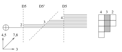
Figure 4: The generalization of $\rho$ when D5 and D5^′ branes are present. We have restricted our attention to the case where the linking number is non-decreasing so that a generalized Young diagram can be drawn as illustrated, although there are no a priori reason to only consider this case.

3 Boundaries with Localized Degrees of Freedom

In the previous section, we saw that a natural class of supersymmetric boundary conditions arose from demanding that the supercurrent have vanishing flux through the boundary. However, this analysis depended on a restrictive assumption, that the only degrees of freedom in the problem live in the bulk. In this section, we will explore some interesting classes of boundary degrees of freedom and the boundary conditions they imply for the bulk fields.

An astute reader might have wondered whether we are required to choose the particular form of the supercurrent in eq. (2.4). Just as is the case for the energy-momentum tensor, we could have considered adding conserved “improvement” terms to the supercurrent. They can generically be constructed by adding total derivative terms to the Lagrangian before implementing the Noether procedure; thus it is clear that they do not affect the local analysis of supersymmetry, but they do affect the global analysis. In particular, the improvement terms are important in the presence of boundaries, where the total derivatives give rise to Lagrangians defined at the boundary, potentially with their own degrees of freedom.

To visualize the kind of construction we want to study, let us start by recalling the construction of ${\cal N}=2$ Abelian theory in 2+1 dimensions using branes. As a concrete example, we show two ways of constructing a theory with $U(1)$ gauge symmetry and $N_{f}=3$ flavors in figure 5.

Figure 5: Brane construction of ${\cal N}=2$ $U(1)$ $N_{f}=3$ theory in two different brane orderings.

Configurations like these were used to engineer ${\cal N}=2$ theories in [20, 25]. The 5-branes and the 3-branes can then be allowed to move, with their positions being interpretable as masses, FI parameters, and components of the moduli. These features are explained in detail in [20, 25].

The two configurations in figure 5 describe equivalent physics in the IR, in that they are related by the exchange of the relative positions of an NS5 brane and the D5 brane. Although what is illustrated in figure 5 is a string theory construct, one can also consider a decoupling limit and think of the system as consisting of defects and boundaries of a gauge field theory in 3+1 dimensions. The distance $L$ between the NS5 and the NS5^′ brane encodes the 2+1 gauge coupling via the relation

$$g_{\rm YM3}^{2}={g_{\rm YM4}^{2}\over L}\ .$$ (3.1)

It is also common to engineer the theory in 2+1 dimensions by pushing the D5 branes infinitely to the right so that the configuration resembles a 3+1 theory bounded by an NS5^′ and an NS. This picture, however, obscures the decoupling between the 2+1 dimensional physics and 3+1 dimensional physics due to light modes living on the segment between the NS5 and the D5^′s. This issue is related to the subtlety in formally defining the notion of the “moduli space of the boundary” as a local notion, independent of the bulk physics and the “boundary condition on the other side.”

Our goal in this section is to specify boundary conditions for ${\cal N}=4$ SYM in a sufficiently precise way that we can compute the moduli space of configurations like the one in figure 5 in terms of an explicit computation for a defect version of the ${\cal N}=4$ theory.

3.1 Bulk Equations

In this section, we will describe the conditions imposed on the bulk fields by supersymmetry.

Before proceeding, we will rewrite the bulk supersymmetry equations (2.31)–(2.38) in a form where holomorphy is manifest: we have 3$d$ $\mathcal{N}=2$ theory and the moduli space is Kähler. A consistent truncation that is sometimes useful to consider is to set $\vec{Y}=0$, and to suppress all terms with Lorentz indices, leaving precisely the Nahm equation (2.81). It will turn out to be convenient to combine $X_{4}$ and $X_{5}$ into complex combination

$${\cal X}\equiv X_{4}+iX_{5}\ ,$$ (3.2)

as well as $A_{3}$ and $X_{6}$ into

$${\cal A}\equiv A_{3}+iX_{6}\ ,$$ (3.3)

so that the two of the three Nahm equations can be written as a complex equation

$$\frac{\mathcal{D}\mathcal{X}}{\mathcal{D}y}\equiv\frac{d\mathcal{X}}{dy}+[\mathcal{A},\mathcal{X}]=0\ ,$$ (3.4)

and the third Nahm equation is

$$\frac{d}{dy}\left(\mathcal{A}-\bar{\mathcal{A}}\right)-\left[\mathcal{A},\bar{\mathcal{A}}\right]+\left[\mathcal{X},\bar{\mathcal{X}}\right]=0\ ,$$ (3.5)

where the barred fields are $\bar{\cal X}\equiv X_{4}-iX_{5}$ and $\bar{\cal A}\equiv A_{3}-iX_{6}$. This is a standard form of presenting the Nahm equation, and can be an effective form for analyzing moduli spaces as quotient space as we will review later in this section.

In the case where only one quarter of supersymmetry (2.60) is preserved, one should generally expect the the $Y$ fields to mix as seen in (2.70)–(2.78). In this case, the useful truncation is to consider is $X_{9}=0$. Then the bulk equations in terms of complex fields are given by three naturally complex equations,

$$\frac{\mathcal{D}\mathcal{X}}{\mathcal{D}y} = 0\ ,$$ (3.6)

$$\frac{\mathcal{D}\mathcal{Y}}{\mathcal{D}y} = 0\ ,$$ (3.7)

$$\left[\mathcal{X},\mathcal{Y}\right] = 0\ ,$$ (3.8)

and one real equation,

$$\frac{d}{dy}\left(\mathcal{A}-\bar{\mathcal{A}}\right)-\left[\mathcal{A},\bar{\mathcal{A}}\right]+\left[\mathcal{X},\bar{\mathcal{X}}\right]+\left[\mathcal{Y},\bar{\mathcal{Y}}\right] = 0\ ,$$ (3.9)

where

$$\mathcal{Y} \equiv X_{7}+iX_{8}\ .$$ (3.10)

In addition to these equations, we also have BPS conditions for the sixth scalar $X_{9}$:

$$D_{3}X_{9} = 0\ ,$$ (3.11)

$$\left[X_{6},X_{9}\right] = 0\ ,$$ (3.12)

$$\left[\mathcal{X},X_{9}\right] = 0\ ,$$ (3.13)

$$\left[\mathcal{Y},X_{9}\right] = 0\ .$$ (3.14)

The equations involving $X_{9}$ do not obey the same division into “naturally real” and “naturally complex” parts as with the other BPS equations; because of this, when $X_{9}$ is nonzero, the correct Kähler structure of the moduli space can be obscured.

One simple class of solutions can be obtained by simply setting $X_{9}=0$, so that the BPS equations are indeed those of a Kähler quotient. In fact this turns out to be the most interesting case, but it is not the most general. For example, we might consider a single D3-brane suspended between two NS5-branes (extended in the 789 directions), for which we would expect that there is indeed a modulus associated with motions of the D3-brane in the $X_{9}$-direction, and also a modulus associated with the “dual scalar” from the reduction of the 4$d$ theory to a 3$d$ theory. This example with NS5-branes is prototypical; the NS5-brane boundary conditions allow $X_{9}$ to contribute to the moduli space, but they also preserve an unbroken abelian gauge symmetry which in this case allows the dual scalar to also be part of the moduli space.

It will turn out that the boundary conditions which preserve some amount of unbroken gauge symmetry are those for which the scalar $X_{9}$ is active. This is a subtle issue when quantum effects are taken into account, but sometimes it can be useful to keep track of the classical moduli associated with $X_{9}$ and the dual scalar, even if they receive quantum corrections.

3.2 Junction Conditions

In order to discuss junction conditions, we need to incorporate the localized degrees of freedom at the D5 and NS5 defects. In the case where the NS5 and D5 break the same half of the supersymmetry, this issue has been worked out in the treatment of GW [1].

Specifically, for the D5 brane at $x^{3}=x^{7}=x^{8}=x^{9}=0$ intersecting $N$ D3-branes, equation (3.27) of [1] reads

$${D\vec{X}\over Dy}+\vec{X}\times\vec{X}+\delta(y)\vec{\mu}_{\omega}=0\ ,$$ (3.15)

and for the NS5-brane at $x_{3}=x_{4}=x_{5}=x_{6}=0$, equation (3.79) of [1] reads

$$-\vec{X}_{L}(0)+\vec{\mu}_{L} = 0\ ,$$ (3.16)

$$\vec{X}_{R}(0)+\vec{\mu}_{R} = 0\ .$$ (3.17)

Here, $\mu_{\omega}$, $\mu_{L}$, and $\mu_{R}$ refers to the contribution of the matter fields localized on the defect to the moment maps. These relations would be all that we need in principle, except for one critical ingredient: in the half BPS case, we usually restrict to the case that $\vec{Y}=0$. When we consider 1/4 BPS configurations, however, it is no longer appropriate to ignore the $\vec{Y}$ fields.

In this subsection, we will review the arguments deriving the junction condition for the $\vec{X}$ and the $\vec{Y}$ fields across the D5 and NS5 domain walls. Along the way we will reproduce the explicit form for the moment functions $\mu_{\omega}$, $\mu_{L}$, and $\mu_{R}$. Once these are worked out, it is straightforward to generalize the junction conditions to the NS5^′ and the D5^′ defects.

3.2.1 D5-like Junction

We begin by reviewing the D5 boundary and defects. We start by considering $N$ D3 branes ending on both sides of a D5-brane interface. The junction condition for $N$ D3 on one side and $M<N$ D3 on the other side of the D5 can be inferred by pushing some of the D3’s to infinity along the world volume of D5. As we have seen already, even for 1/4 BPS cases the junction condition at the D5-brane is 1/2 BPS, which was already discussed in [1]. However for the application to the 1/4 BPS cases it is crucial to work out the conditions of all the scalars involved, in particular $\mathcal{Y}$.

It is intuitively clear that there are some modes localized at the D3-D5 intersection, when $M=N$: these are the the strings connecting D3 and D5-branes. From the viewpoint of the D3-brane the strings give rise to a chiral multiplet $Q$ in the fundamental representation or $\tilde{Q}$ in the anti-fundamental representation, depending on the orientation of the strings. Since the D3-D5 intersection locally is 1/2 BPS, $Q$ and $\tilde{Q}$ combine to form a 3$d$ $\mathcal{N}=4$ hypermultiplet ${\omega}=(Q,\tilde{Q})$.

The localized fields $Q,\tilde{Q}$ should couple to the bulk degrees of freedom. For this purpose we can write the fields of 4$d$ $\mathcal{N}=4$ SYM in terms of 3$d$ $\mathcal{N}=2$ superspace, following the formalism of [26, 27].

The 4$d$ $\mathcal{N}=4$ vector multiplet can be decomposed into four 3$d$ $\mathcal{N}=2$ multiplets. First, we have one $\mathcal{N}=2$ vector multiplet $V$, or rather the associated linear multiplet

$$\Sigma=\frac{1}{2i}\epsilon^{\alpha\beta}\bar{D}_{\alpha}(e^{-V}D_{\beta}e^{V})\ ,$$ (3.18)

which contains the topological current $J^{\mu}\equiv\frac{1}{2}\epsilon^{\mu\nu\rho}F_{\nu\rho}$ in one of its components. Here the role of the vector multiplet adjoint scalar is played by the adjoint scalar $X_{9}$. Second, we have three $\mathcal{N}=2$ chiral multiplets $\mathcal{A},\mathcal{X},\mathcal{Y}$, which are the complex combinations of $A_{3}$ and $X_{4,5,6,7,8}$. The latter three coincide with our previous definition given in (3.2),(3.3), and (3.10). Each of these four $\mathcal{N}=2$ multiplets depends on the $y$-coordinate.

We can write the bulk $\mathcal{N}=4$ Lagrangian in terms of 3$d$ $\mathcal{N}=2$ superfields. The answer is given by [27]

$$\begin{split}\mathcal{L}_{\rm bulk}&=\int d^{4}\theta\,\textrm{Tr}\left[\Sigma^{2}+\frac{1}{2}(e^{-V}\bar{\mathcal{D}}e^{V}+\mathcal{A})^{2}-e^{-V}\bar{\mathcal{X}}e^{V}\mathcal{X}-e^{-V}\bar{\mathcal{Y}}e^{V}\mathcal{Y}\right]\\ &\qquad+\int d^{2}\theta\,\textrm{Tr}\left(\mathcal{X}\mathcal{D}\mathcal{Y}-\mathcal{Y}\mathcal{D}\mathcal{X}\right)+\int d^{2}\bar{\theta}\,\textrm{Tr}\left(-\bar{\mathcal{X}}\bar{\mathcal{D}}\bar{\mathcal{Y}}+\bar{\mathcal{Y}}\bar{\mathcal{D}}\bar{\mathcal{X}}\right)\ ,\end{split}$$ (3.19)

where $\mathcal{D}\equiv\partial_{y}+\mathcal{A},\bar{\mathcal{D}}\equiv\partial_{y}+\bar{\mathcal{A}}$ as in (3.4). Recall that in our convention $\mathcal{A},\mathcal{X},\mathcal{Y}$ are anti-Hermitian and hence for example $\mathcal{X}^{\dagger}=-\bar{\mathcal{X}}$.

Note that the $F$-term contains the commutator term $\textrm{Tr}([\mathcal{X},\mathcal{Y}]\mathcal{A})$, which is related to the superpotential term of the 4$d$ $\mathcal{N}=4$ theory. Note also that the $F$-term equations for this bulk Lagrangian give

$$\mathcal{D}\mathcal{X}=\mathcal{D}\mathcal{Y}=0$$ (3.20)

which are nothing but the complex part of the Nahm equations.

We can also vary the vector multiplet $V$ in (3.19), and if we neglect the covariant derivatives along the 3$d$ directions we have the real part of the Nahm equations.

Let us now come back to the coupling with the $Q,\tilde{Q}$. The coupling between the bulk and the boundary should preserve 3$d$ $\mathcal{N}=4$ supersymmetry. This determines the bulk-boundary interaction to be

$$\mathcal{L}_{\rm defect}=\left[\int d^{4}\theta\left(Q^{\dagger}e^{V}Q+\tilde{Q}e^{-V}\tilde{Q}^{\dagger}\right)+\int\!d^{2}\theta\,\left[\tilde{Q}\mathcal{Y}Q\right]-\int\!d^{2}\bar{\theta}\,\left[Q^{\dagger}\bar{\mathcal{Y}}\tilde{Q}^{\dagger}\right]\right]\delta(y-y_{0})\ ,$$ (3.21)

where $y_{0}$ represents the position of the defect along the $y$-direction. This takes the form of the Lagrangian of 3$d$ $\mathcal{N}=4$ theory, where the role of the adjoint 3$d$ $\mathcal{N}=2$ chiral (vector) multiplet is played by the bulk chiral multiplet $\mathcal{Y}$.

Note that the superpotential term $\tilde{Q}\mathcal{X}Q$ has the correct dimension $2$; this is because the bulk field $\mathcal{Y}$, being a field in four dimensions, has mass dimension $1$ ($Q$ and $\tilde{Q}$ have canonical mass dimension in 3$d$, namely $1/2$).

Let us now see how this affects our analysis of the moduli space. When we vary the bulk fields, the equations of motion for the bulk fields read

$$V:\quad\frac{d}{dy}(\mathcal{A}-\bar{\mathcal{A}})-[\mathcal{A},\bar{\mathcal{A}}]+[\mathcal{X},\bar{\mathcal{X}}]+[\mathcal{Y},\bar{\mathcal{Y}}]+\mu_{\omega,\mathbb{R}}\,\delta(y-y_{0})=\zeta\ ,$$ (3.22)

$$\mathcal{X}:\quad\frac{\mathcal{D}\mathcal{X}}{\mathcal{D}y}+\,\mu_{\omega,\mathbb{C}}\,\delta(y-y_{0})=0\ ,$$ (3.23)

and $\mu_{\mathbb{R}},\mu_{\mathbb{C}}$ are real and complex moment maps defined by

$$\mu_{\omega,\mathbb{R}} \equiv QQ^{\dagger}-\tilde{Q}^{\dagger}\tilde{Q}\ ,$$ (3.24)

$$\mu_{\omega,\mathbb{C}} \equiv Q\tilde{Q}\ .$$ (3.25)

We can combine these equations into

$$D_{y}X_{a}-\frac{1}{2}\epsilon_{abc}[X_{b},X_{c}]-\mu_{\omega,a}\delta(y-y_{0})=0\ ,$$ (3.26)

where

$$\omega\equiv\frac{1}{\sqrt{2}}\left(\begin{array}[]{cc}Q&\tilde{Q}^{{\dagger}}\end{array}\right)\ ,\qquad\omega^{{\dagger}}\equiv\frac{1}{\sqrt{2}}\left(\begin{array}[]{c}Q^{{\dagger}}\\ \tilde{Q}\end{array}\right)\ ,$$ (3.30)

and

$$\vec{\mu}_{\omega}\equiv\omega^{{\dagger}}\vec{\sigma}\omega$$ (3.31)

is a triplet of moment maps, making manifest the hyperKähler structure (which comes from 3$d$ $\mathcal{N}=4$ supersymmetry locally present at the junction.) Note that the triplet structure is not manifest in the 3$d$ $\mathcal{N}=2$ superspace formulation, see however appendix B for a 3$d$ $\mathcal{N}=1$ superspace formulation which makes the triplet structure manifest.

The moment maps $\vec{\mu}_{\omega}$ cause $\vec{X}_{a}$ to jump at the D5 and are sometimes referred to as the “jumping conditions.” Two of the three components of $\vec{\mu}_{\omega}$ can also be found in (3.33) of [1]. The equations are known in the context of the Nahm equations, see [28] and also [29, 30].

In general the supersymmetry is broken to 1/4 BPS with other boundary/junction conditions, and we have only 3$d$ $\mathcal{N}=2$ superspace. Even in these cases, the $F$-term part is protected from perturbative quantum corrections thanks to the non-renormalization theorem for 3$d$ $\mathcal{N}=2$ theory.

There is an additional constraint imposed on the fields $\mathcal{Y}$ due to the superpotential (3.21). The $F$-term equation for the fields $Q,\tilde{Q}$ gives

$${\cal Y}Q =0\ ,$$ (3.32)

$$\tilde{Q}{\cal Y} =0\ .$$ (3.33)

This is part of the triplet of the equations (see appendix B)

$$Y_{a}\sigma^{a}\omega=\omega^{{\dagger}}Y_{a}\sigma^{a}=0\ ,$$ (3.34)

which includes extra conditions

$$Y_{3}Q=\tilde{Q}Y_{3}=0\ .$$ (3.35)

For the most part, we can consistently set

$$Y_{3}=X_{9}=0$$ (3.36)

for both half and quarter supersymmetric cases. Exceptions will be discussed briefly below, but as long as $Y_{3}$ is set to zero, the constraint on $X$ and $Y$ can be written more concisely as

$$\Delta\mathcal{X}(y_{0}) = Q\tilde{Q}\ ,$$ (3.37)

$$i\Delta X_{6} = QQ^{{\dagger}}-\tilde{Q}^{{\dagger}}\tilde{Q}\ ,$$ (3.38)

$${\cal Y}Q = 0\ ,$$ (3.39)

$$\tilde{Q}{\cal Y} = 0\ .$$ (3.40)

We see that the new conditions (3.39), (3.40) imply that $\mathcal{X}$ is only allowed to jump if $\mathcal{Y}=0$, or in other words, when the D3-branes intersect the D5-brane.

With these ingredients, one can easily understand the case of $N$ D3-branes on one side and $N-1$ on the other by considering limiting forms of the fundamental quarks $Q,\tilde{Q}$ (this essentially follows the analysis of [31] in the context of monopole solutions.) One possibility is to parametrize

$${\cal X}_{L}=\left(\begin{array}[]{ccc|c}&&&{}\hfil\\ &A&&B\\ &&&{}\hfil\\ \hline\cr&C&&D\end{array}\right),\qquad{\cal X}_{R}=\left(\begin{array}[]{ccc|c}&&&{}\hfil\\ &A^{\prime}&&0\\ &&&{}\hfil\\ \hline\cr&0&&\alpha\end{array}\right)\ ,$$ (3.41)

with

$$Q^{\dagger}=(u_{1},\ldots u_{N-1},M)\ ,\qquad\tilde{Q}=(v_{1},\ldots v_{N-1},M)\ .$$ (3.42)

We can then solve (3.37) by setting

$$|M^{2}|=\alpha-D\ ,\qquad u_{i}={\lambda\over M}B^{*}_{i}\ ,\qquad v_{i}={1\over\lambda^{*}M^{*}}C_{i}\ .$$ (3.43)

We can consider the case

$$i\Delta X_{6}=QQ^{\dagger}-\tilde{Q}^{\dagger}\tilde{Q}=0\ ,$$ (3.44)

which amounts to not moving the D3’s in the $X_{6}$ direction to fix $\lambda$. These two conditions determine $Q$ and $\tilde{Q}$ completely up to the phase of $\lambda$ and $M$. These phases, however, are irrelevant when we take the limit $|M|\rightarrow\infty$. In that limit, $Q$ and $\tilde{Q}$ are determined uniquely. Also, in that limit, we find that the $(N-1)\times(N-1)$ block

$$A=A^{\prime}$$ (3.45)

is continuous. Finally, we observe that in the limit, $B$, $C$, and $D$ are arbitrary. This is the same feature found in (3.42) and (3.43) of [1].

The D5-brane interface conditions imply restrictions on the allowed gauge transformations when the numbers of D3-branes on each side of the interface are unequal. Specifically, the form (3.42) only preserves a $U(N-1)$ gauge symmetry of the bulk $U(N)$; note also that because some of the fields are continuous across the interface, the gauge transformations must also be continuous. We see that the allowed gauge transformations take the block form

$$g=\left(\begin{array}[]{ccc|c}&&&{}\hfil\\ &*&&0\\ &&&{}\hfil\\ \hline\cr&0&&1\end{array}\right).$$ (3.50)

The other structure that we need is the condition imposed on the $Y$ fields. This was covered only implicitly in [1] but we can read off the relevant detail from (3.39) and (3.40). Since one component of $Q$ and $\tilde{Q}$ is blowing up while the others are going to zero, we infer that the row and the column of ${\cal Y}$ associated with the divergent component of $Q$ and $\tilde{Q}$ must vanish. Physically, this is simply the statement that the D3 brane ending on a D5 brane must have its transverse coordinates coincident with the transverse coordinate of the D5-brane.

Now that we have worked out the case of D5 junction with $N$ D3 on one side and $N-1$ on the other, we can extend to the case with $N$ on one side and $N-M$ on the other with $M>1$. For the ${\cal X}$ fields, the structure is similar to (3.41) except that now, $B$ and $C$ are $M\times(N-M)$ and $D$ is $M\times M$. $B$ and $C$ are required to be finite, whereas $D$ will have the structure of Nahm poles close to the D5 brane. In the limit $M=N$, $A$, $B$, and $C$ goes away and we have the standard Nahm pole boundary condition. These are basically the findings reported in [1]. We also impose the condition that the $N-M$ rows and column of ${\cal Y}$ field vanish.

We close this subsection by pointing out that this analysis can easily be extended to the junction condition for the D5^′ brane oriented along the 012678 direction. They are related to the case of D5-brane oriented along 012456 simply by exchanging ${\cal X}$ and ${\cal Y}$ while leaving $X_{6}$ alone:

$$\Delta\mathcal{Y}(y_{0}) = Q\tilde{Q}\ ,$$ (3.51)

$$i\Delta X_{6} = QQ^{{\dagger}}-\tilde{Q}^{{\dagger}}\tilde{Q}\ ,$$ (3.52)

$${\cal X}Q = 0\ ,$$ (3.53)

$$\tilde{Q}{\cal X} = 0\ .$$ (3.54)

3.2.2 NS5-like Junction

Next, let us turn our attention to the case of NS5-branes intersecting $N$ D3-brane from the left and $M$ D3-branes from the right. There should again be localized degrees of freedom, this time representing the strings between D3-branes on the left and on the right. They are bifundamentals under the $U(N)\times U(M)$ gauge symmetry; we have $\mathcal{N}=2$ bifundamental chiral multiplets $A$ and $B$ transforming as (${\bf N,\bar{M}}$) and (${\bf\bar{N},M}$), which together make up an $\mathcal{N}=4$ hypermultiplet.

We can again write down the Lagrangian representing the coupling of the localized field $A,B$ to the bulk:

$$\mathcal{L}_{\rm defect} =\delta(y-y_{0})\int d^{4}\theta\left(\textrm{Tr}_{R}A^{\dagger}e^{V_{L}}Ae^{V_{R}}+\textrm{Tr}_{L}B^{\dagger}e^{V_{R}}Be^{V_{L}}\right)$$

$$\quad+\delta(y-y_{0})\left(\int d^{2}\theta\left[\textrm{Tr}_{L}AB\mathcal{Y}_{L}+\textrm{Tr}_{R}BA\mathcal{Y}_{R}\right]+\textrm{(h.c.)}\right)\ ,$$ (3.55)

where as before $y_{0}$ represents the position of the defect along the $y$-direction. Note that again this interaction is completely fixed by the requirement of 3$d$ $\mathcal{N}=4$ supersymmetry We can check that the superpotential terms have correct dimension $2$, since $A$, $B$ have 3$d$ canonical dimension $1/2$, whereas the bulk fields $\mathcal{X},\mathcal{Y}$ dimension $1$.

We can derive the junction conditions again from (3.2.2). However, some care is needed since there is also a boundary contribution from the bulk Lagrangian (3.19), which contains the term, after integrating by parts,

$$\int d^{3}x\int_{y<y_{0}}\!dy\,\textrm{Tr}(\mathcal{X}_{L}\mathcal{D}\mathcal{Y}_{L}-\mathcal{Y}_{L}\mathcal{D}\mathcal{X}_{L})=\int d^{3}x\int_{y<y_{0}}\!dy\,\textrm{Tr}(2\mathcal{X}_{L}\mathcal{D}\mathcal{Y}_{L})-\int d^{3}x\,\textrm{Tr}\,\mathcal{X}_{L}\mathcal{Y}_{L}\Big{|}_{y=0}\ .$$ (3.56)

The integration by parts are done in such a way that the bulk contribution vanishes at the boundary in light of ${\cal DY}$ being zero at the interface. When we have no localized degrees of freedom at the boundary, we should impose $\mathcal{X}_{L}=0$ on the NS5-like boundary and hence (3.56) vanishes. However for our purposes $\mathcal{X}_{L}=0$ turns to be too strong, and we should keep the boundary contribution $\textrm{Tr}\,\mathcal{X}_{L}\mathcal{Y}_{L}$. There is also a similar contribution from the region $y>y_{0}$ (this time with the opposite sign due to orientation reserval), and collecting there we have the boundary contribution from the bulk:

$$\mathcal{L}_{\partial\textrm{(bulk)}}=\int d^{2}\theta\,\textrm{Tr}\,\left[-\mathcal{X}_{L}\mathcal{Y}_{L}+\mathcal{X}_{R}\mathcal{Y}_{R}\right]\delta(y-y_{0})\ .$$ (3.57)

We can now derive the $F$-term constraints, which gives the same equations as in (3.79) and (3.80) of [1]:

$${\cal X}_{L} =\mu_{L,\mathbb{C}}\equiv AB\ ,$$ (3.58)

$${\cal X}_{R} =-\mu_{R,\mathbb{C}}\equiv-BA\ .$$ (3.59)

We can again supplement (3.58)–(3.59) by the equation involving real part of the triplet of the moment maps, making the hyperKähler structure at the junction manifest (c.f. appendix B):

$$iX_{6,L} = \mu_{L,\mathbb{R}}\equiv AA^{\dagger}-B^{\dagger}B\ ,$$ (3.60)

$$iX_{6,R} = \mu_{R,\mathbb{R}}\equiv A^{\dagger}A-BB^{\dagger}\ ,$$ (3.61)

where the we have introduced the real part of the triplet of moment maps defined similarly to the D3-D5 case:

$$\mu_{L}=\xi Y_{L}^{a}\sigma^{a}\xi^{\dagger},$$ (3.62)

with

$$\xi=\frac{1}{\sqrt{2}}\left(\begin{array}[]{c}A^{{\dagger}}\\ B\end{array}\right),\qquad\xi^{{\dagger}}=\frac{1}{\sqrt{2}}\left(\begin{array}[]{cc}A&B^{{\dagger}}\end{array}\right)\ .$$ (3.66)

We also have the $F$-term equation from the fields $A$ and $B$:

$$B:\mathcal{Y}_{L}A-A\mathcal{Y}_{R} = 0\ ,$$ (3.67)

$$A:B\mathcal{Y}_{L}-\mathcal{Y}_{R}B = 0\ .$$ (3.68)

Note that the $F$-term equation for the field $\mathcal{X}$ gives complex part of

$$D_{3}Y_{L}^{a}=Y_{L}^{a}\delta(y-y_{0})\ ,$$ (3.69)

which effectively states that $Y_{L}^{a}$ is gauge-covariantly-constant in the bulk and takes an arbitrary value at the boundary. This is just what one expects for a D3-brane ending on an NS5-brane. Similar conclusion applies to $Y_{R}^{a}$.

Crucially, because the fields are not required to be continuous across an NS5-interface, we have independent gauge symmetries acting on each side (unlike the D5-brane boundary condition.) This is necessary so that the D3-brane segments between any pair of NS-type branes give rise to an independent 3-dimensional gauge symmetry.

To summarize, at NS5 oriented along 012789 with $N$ D3 ending from the left and $M$ D3 ending from the right, we impose the junction conditions

$${\cal X}_{L} = AB\ ,$$ (3.70)

$${\cal X}_{R} = BA\ ,$$ (3.71)

$$iX_{6,L} = AA^{\dagger}-B^{\dagger}B\ ,$$ (3.72)

$$iX_{6,R} = A^{\dagger}A-BB^{\dagger}\ ,$$ (3.73)

$$\mathcal{Y}_{L}A = A\mathcal{Y}_{R}\ ,$$ (3.74)

$$B\mathcal{Y}_{L} = \mathcal{Y}_{R}B\ .$$ (3.75)

To gain some intuition for these equations, consider the case where the gauge group is $U(N)$ on the left, and $U(1)$ on the right. Then $A$ and $B$ are constrained to be either a row or column eigenvector of $\mathcal{Y}_{L}$. If $A,B$ do not both vanish, then $\mathcal{Y}_{R}$ (which is a complex scalar) is equal to one of the eigenvalues of $\mathcal{Y}_{L}$, and generic expectation values for $A$ or $B$ will break all the gauge symmetry at the interface. However, if $A$ and $B$ do both vanish, there is no constraint and $\mathcal{Y}_{R}$ can take any value. In this latter case, $U(N)$ is only broken to $U(1)^{N}$ by generic expectation values for $\mathcal{Y}_{L}$. We see also that $\mathcal{X}$ is only allowed to jump if some of the D3-branes are continuous across an NS5 interface.

We can also generalize these conditions for the case of NS5^′ brane junction oriented along 012459 by exchanging ${\cal X}$ and ${\cal Y}$.

$${\cal Y}_{L} = AB\ ,$$ (3.76)

$${\cal Y}_{R} = BA\ ,$$ (3.77)

$$iX_{6,L} = AA^{\dagger}-B^{\dagger}B\ ,$$ (3.78)

$$iX_{6,R} = A^{\dagger}A-BB^{\dagger}\ ,$$ (3.79)

$$\mathcal{X}_{L}A = A\mathcal{X}_{R}\ ,$$ (3.80)

$$B\mathcal{X}_{L} = \mathcal{X}_{R}B\ .$$ (3.81)

3.2.3 Mass/FI Deformations

So far, we have assumed all the 5-branes to be located at the origin in the transverse coordinates. It is however possible to consider generalizations where we move the position of these D5 branes. These deformations are interpretable as Fayet-Iliopolous terms and quark masses of the low energy field theory and was mapped out in [20]. These deformations also have the effect of slightly modifying the junction condition.

For example, for D5-branes which are extended in the 456 directions, so far we have assumed that they are located at $x^{7,8,9}=0$. Displacing a D5-brane in the 78 directions can naturally be implemented by modifying the boundary conditions

$$(\mathcal{Y}-m_{\mathbb{C}}\mathbb{I})Q=\tilde{Q}(\mathcal{Y}-m_{\mathbb{C}}\mathbb{I})=0\ ,$$ (3.82)

which can be reproduced from extra defect superpotential

$$\delta\mathcal{L}_{\rm defect}=m_{\mathbb{C}}\tilde{Q}Q\ .$$ (3.83)

We can also include real mass terms, giving expectation values to $X_{9}$. However since the real mass term is in the $D$-term, it is expected that the precise form of the equation can be corrected quantum mechanically.

For NS5-branes, the position of the NS5-brane gives the FI parameter, which modifies the bulk Lagrangian (3.19) by the standard $D$-term $\mathcal{L}_{\rm FI}=\int d^{4}\theta\,\zeta V$. This naturally gives

$$iX_{6,L} = AA^{{\dagger}}-B^{{\dagger}}B+\zeta_{\mathbb{R}}\mathbb{I}_{L}\ ,$$ (3.84)

$$iX_{6,R} = A^{{\dagger}}A-BB^{{\dagger}}+\zeta_{\mathbb{R}}\mathbb{I}_{R}\ ,$$ (3.85)

for the real part, which is supplemented by the complex counterparts

$$\mathcal{X}_{L} = AB+\zeta_{\mathbb{C}}\mathbb{I}_{L}\ ,$$ (3.86)

$$\mathcal{X}_{R} = BA+\zeta_{\mathbb{C}}\mathbb{I}_{R}\ .$$ (3.87)

In general, there can be quantum corrections to the real equations involving $X_{6}$. We have defined $\mathbb{I}_{L}$ and $\mathbb{I}_{R}$ as the identity matrices on the left-hand and right-hand sides of the NS5-brane. Of course there are analogous expressions for the NS5^′-brane boundary conditions.

In analyzing 2+1 field theories with ${\cal N}=2$ supersymmetries, it will be instructive to explore how the moduli space depends on these deformation parameters.

3.3 Moduli Space and Complexified Gauge Symmetry

A powerful technique which we will employ in analyzing the moduli space of some of these boundary/defect systems is to complexify the gauge symmetry. The essential idea behind this technique is that because the moduli space is a Kähler quotient, it can be computed by promoting the gauge group $G$ to a complexified gauge group $G_{\mathbb{C}}$ (modulo the issue of stability [32] which will turn out to be important in the analysis of 3$d$ gauge theory [9]). A discussion of this technique in the context of the Nahm equations can be found in [33].

To determine the moduli space, the mathematical problem of interest is that of solving a set of differential equations (3.6), (3.7), and (3.9) subject to an algebraic constraint (3.8) and the boundary and junction conditions (which are also algebraic), and up to gauge equivalence under the gauge group $G$. This problem can be solved directly, but we can take advantage of the fact that some of the equations, such as the differential equations (3.6), (3.7), (3.8), and some of the boundary conditions, are manifestly in a complex form. These complex equations are actually invariant under a larger gauge symmetry group than the full set of equations – we may take $\mathcal{X}\rightarrow g^{-1}\mathcal{X}g$, $\mathcal{Y}\rightarrow g^{-1}\mathcal{Y}g$, $\mathcal{A}\rightarrow g^{-1}\mathcal{A}g+g^{-1}dg$, where $g$ is valued in the complexified gauge group $G_{\mathbb{C}}$. On the other hand, the real equation (3.9) is only invariant under the real gauge symmetry $G$ and transforms nontrivially under $G_{\mathbb{C}}$.

It is a beautiful mathematical fact that solving the full system of equations (3.6)–(3.9), modded out by the gauge symmetry $G$, is equivalent to solving the complex system (3.6)–(3.8), modded out by the complexified gauge symmetry $G_{\mathbb{C}}$, and where we completely ignore the real equation (3.9). The technical point is that for a particular choice of $G_{\mathbb{C}}$ gauge, a typical solution of the complex equations will not solve the real equation, but because (3.9) transforms under $G_{\mathbb{C}}$, there will be a gauge-equivalent point which does solve the real equation. As a practical matter, this procedure of using $G_{\mathbb{C}}$ and ignoring the real equation proves to be a drastic technical simplification.

3.4 Summary of Section 3

Let us pause to summarize the main results of section 3. In this section, we have explicitly worked out

• Generalized Nahm equations (3.6)–(3.9),

• Junction condition for D5 (3.37)–(3.40) and for D5^′ (3.51)–(3.54),

• Junction condition for NS5 (3.70)–(3.75) and for NS5^′ (3.76)–(3.81).

The moduli space of field configurations subject to the boundary conditions consists of solutions to these equations modulo gauge equivalences. To make this notion completely precise, we need to specify the boundary/junction condition also for the gauge parameters. On D5 junctions with the same number of D3’s on each sides, we will require the gauge parameter to be continuous [34]. On NS5-branes, where bifundamental degrees of freedom live, we allow the gauge parameter to be discontinuous and take arbitrary values on either side.

We have also described how the Kähler structure comes about naturally from the complexified gauge formalism. These relations will be the main ingredient for our subsequent analysis in the remainder of this paper as well as in the companion paper [9].

4 Boundary Conditions on a Half-Space

A particularly simple class of boundary conditions are those which are defined on a half-space; that is, we take the ${\cal N}=4$ theory defined in $\mathbb{R}^{3,1}$ but restricted to $x^{3}=y>0$. At $y=0$, we impose some conditions on the bulk fields consistent with the amount of supersymmetry we wish to preserve. This proves to be a simple context in which we can understand the issues which arise from reducing to supersymmetry to 1/4 BPS.

We will describe two important classes of boundary conditions – those which can be constructed from a sequence of D5 and D5^′ branes, which we can think of as a generalization of Dirichlet boundary conditions, and their S-duals, which we can construct from a sequence of NS5 and NS5^′-branes. We will see that the various boundary conditions impose different constraints on the bulk fields.

The spaces of bulk field configurations allowed by a given boundary condition are similar to moduli spaces, but to give a truly well-posed problem for the field configurations on a half-space we need to also specify a boundary condition at infinity. In GW [1] a canonical choice of boundary condition at infinity was used, namely that the $\vec{X}$ fields should be valued in a maximal torus of the gauge group, with the $\vec{Y}$ fields all set to zero. As it turns out, this boundary condition is equivalent to coupling the theory on a finite interval to a quiver gauge theory $T[SU(N)]$. This quiver gauge theory admits a 1/4 BPS generalization which we will describe.

Throughout this section, we will place D5-branes at the origin of $X_{7,8,9}$ and D5^′-branes at the origin of $X_{4,5,9}$ for simplicity; generic positions can be easily restored.

In this section we start with a 1/2 BPS boundary conditions in section 4.1. We then discuss 1/4 BPS boundary conditions in sections 4.2 and 4.3, starting with simple examples and then moving on to more complicated examples.

4.1 1/2 BPS Boundary Conditions

We review briefly some of the boundary conditions discussed in [1].

4.1.1 Ordinary Dirichlet Boundary Conditions

First, let us recall what GW called the “ordinary” Dirichlet boundary condition for $U(N)$ $\mathcal{N}=4$ SYM. For the theory realized on $N$ D3-branes, it corresponds to having a stack of $N$ D5-branes, with one D3-brane ending on each D5-brane. For $N=2$ and $N=3$, the corresponding configuration is shown in figure 6.

Figure 6: Ordinary Dirichlet boundary conditions for $U(2)$ and $U(3)$ gauge theory in the bulk.

We assume that the fields are non-singular throughout the half-space $y>0$, so that we can choose the $G_{\mathbb{C}}$ gauge $\mathcal{A}=0$. The conditions imposed on the scalars $\mathcal{X}$ and $\mathcal{Y}$ are that $\mathcal{X}$ takes any finite value while $\mathcal{Y}=0$.

This boundary condition plays a central role in the discussion of S-duality in [2]. There it was called an “ungauging,” because it removes the gauge fields at low energies but imposes no other constraint on the scalar field $\mathcal{X}$.

4.1.2 1/2 BPS $U(2)$ Boundary with a Pole

The simplest example where we allow a Nahm pole singularity arises for a bulk gauge group $U(2)$. This is the case illustrated in figure 7.

In the analysis of Dirichlet boundary conditions, we chose the gauge $\mathcal{A}=0$. If the boundary has a pole we cannot choose this gauge because we only allow non-singular gauge transformations. However, we are allowed to gauge away all the non-singular terms in $\mathcal{A}$ , leaving us with

$$\mathcal{A}=\frac{it_{3}}{y}\ ,$$ (4.1)

where $t_{3}$ is the Cartan generator of an $\mathfrak{sl}(2)$ subalgebra in the gauge algebra. We satisfy Nahm’s equations with

$$\mathcal{X}=\frac{t_{+}}{y}+({\rm nonsingular})\ .$$ (4.2)

The normalization of the singular part is determined by the singular terms in the third Nahm equation.

We need to solve the BPS equation $\mathcal{D}\mathcal{X}=0$. There are residual gauge transformations satisfying $g(0)=1$; after modding these out we can put $\mathcal{X}$ in the form

$$\mathcal{X}=\left(\begin{array}[]{cc}a&1/y\\ by&a\end{array}\right)\ .$$ (4.5)

We are left with two complex parameters, $a$ and $b$.

From the action of S-duality in string theory, it is clear that the Nahm pole boundary condition is S-dual to a D3-brane ending on an NS5-brane, which gives ordinary Neumann boundary conditions (with no added degrees of freedom.)

Figure 7: $U(2)$ with D5-like boundary giving rise to an elementary Nahm pole.

4.2 1/4 BPS Dirichlet Boundary Conditions

The simplest generalization of the 1/2 BPS Dirichlet boundary conditions is obtained by rotating some of the D5-branes to D5^′-branes. Despite their simplicity, these boundary conditions will already illustrate an important point — unlike the 1/2 BPS case, there is no canonical ordering of the 5-branes in the mixed D5-D5^′ system. This means, in particular, that these boundary conditions do not have a simple classification in terms of Young diagrams of the type illustrated in figure 3.

We consider some concrete examples for $U(2)$ and $U(3)$ gauge theory in the bulk. We begin with boundary conditions without Nahm poles; for these we can consistently choose the $G_{\mathbb{C}}$ gauge $\mathcal{A}=0$. Then the bulk equations are trivial except for the commutator $[\mathcal{X},\mathcal{Y}]=0$.

4.2.1 D5-D5^′ Boundary Conditions for $U(2)$ Gauge Theory

A natural class of 1/4 BPS generalizations of the ordinary Dirichlet boundary condition can be obtained by rotating some of the D5-branes to D5^′-branes; it is particularly interesting because, like the 1/2 BPS ordinary Dirichlet condition, it acts on the vectors as an ungauging. The simplest such boundary condition arises in $U(2)$ $\mathcal{N}=4$ gauge theory. The brane configuration is shown in figure 8.

Figure 8: Dirichlet boundary conditions for D5 and D5^′ branes in $U(2)$ gauge theory.

We construct the boundary conditions from left to right. Beginning with the leftmost gauge theory segment, we have

$$\mathcal{X}=\left(a\right)\ ,\qquad\qquad\mathcal{Y}=\left(0\right)\ ,$$ (4.6)

Proceeding to the $U(2)$ region, $\mathcal{X}$ grows an extra row and column which vanish:

$$\mathcal{X}=\left(\begin{array}[]{cc}a&0\\ 0&0\end{array}\right)\ ,$$ (4.9)

but $\mathcal{Y}$ grows without constraint:

$$\mathcal{Y}=\left(\begin{array}[]{cc}0&b\\ c&d\end{array}\right).$$ (4.12)

Now we impose $[\mathcal{X},\mathcal{Y}]=0$ to find

$$ba=ca=0\ ,$$ (4.13)

and there are two solution branches. The first branch has $b=c=0$:

$$\mathcal{X} = \left(\begin{array}[]{cc}a&0\\ 0&0\end{array}\right)\ ,$$ (4.16)

$$\mathcal{Y} = \left(\begin{array}[]{cc}0&0\\ 0&d\end{array}\right)\ .$$ (4.19)

For this branch, we have only diagonal elements.

The other branch has $a=0$ with no constraints on $b,c,d$:

$$\mathcal{X} = \left(\begin{array}[]{cc}0&0\\ 0&0\end{array}\right)\ ,$$ (4.22)

$$\mathcal{Y} = \left(\begin{array}[]{cc}0&b\\ c&d\end{array}\right)\ .$$ (4.25)

It is instructive to interpret the field configurations for $\mathcal{X}$ and $\mathcal{Y}$ in terms of the allowed motions of branes, as shown in in figure 9. We have indicated each adjustable complex degree of freedom with a green double arrow. We can see that how two parameters, $a$ and $d$ affect the first branch and three parameters, $b$, $c$, and $d$ affect the second branch. Some of these parameters affect the configuration of the brane far from the boundary. The data encoding the position of the semi-infinite D3 branes in the $X_{6}$ direction are not clearly reflected in this presentation because of our choice of $G_{\mathbb{C}}$ gauge. In particular, note that (4.25) is not diagonal. The $X_{6}$ data are encoded in the off-diagonal terms, and can be extracted by choosing a different gauge. In general these data are not totally geometric, because if the “physical” gauge has $\mathcal{A}\neq 0$, the scalars will not necessarily commute.

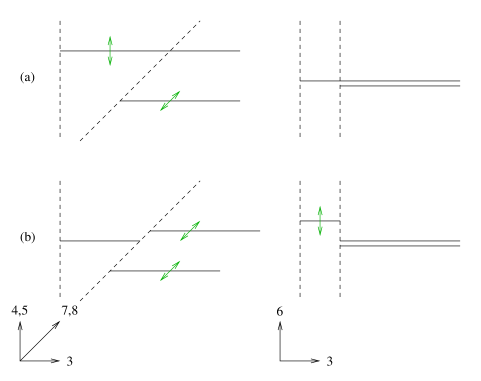
Figure 9: Brane configuration associated with the branch (4.16)–(4.19) on top, and the branch (4.22)–(4.25) on the bottom. The positions of the semi-infinite D3 branes in the $X_{6}$ direction are obscured in the analysis in the main text. They can be recovered by finding the $G_{\mathbb{C}}$ gauge transformation which solves the real part of the Nahm equations.

Of course, interchanging the D5 and D5^′ corresponds to interchanging $\mathcal{X}$ and $\mathcal{Y}$, and this illustrates an important point – after the exchange of the D5 and D5^′, different boundary conditions are imposed on the bulk fields. In general, this will give rise to a phase transition in the moduli space of vacua.

4.2.2 $U(3)$ Examples without Poles

Now we turn to the examples in figure 10. These analyses are included mainly to illustrate our methods to broader set of examples. We consider (a), (b), and (c) in turn.

Figure 10: Possible arrangements of D5 and D5^′ branes boundary conditions for $U(3)$ gauge theory on a half-space.

D5-D5-D5^′

Starting from the left, we have a $U(2)$ gauge theory with ordinary Dirichlet boundary conditions

$$\mathcal{X} = \left(\begin{array}[]{cc}a&b\\ c&d\end{array}\right)\ ,$$ (4.28)

$$\mathcal{Y} = \left(\begin{array}[]{cc}0&0\\ 0&0\end{array}\right)\ .$$ (4.31)

Crossing the D5^′-brane, these become

$$\mathcal{X} = \left(\begin{array}[]{ccc}a&b&0\\ c&d&0\\ 0&0&0\end{array}\right)\ ,$$ (4.35)

$$\mathcal{Y} = \left(\begin{array}[]{ccc}0&0&u\\ 0&0&v\\ r&s&t\end{array}\right)\ .$$ (4.39)

The commutation $[\mathcal{X},\mathcal{Y}]=0$ then gives the equations

$$\left(\begin{array}[]{cc}a&b\\ c&d\end{array}\right)\left(\begin{array}[]{c}u\\ v\end{array}\right) = 0\ ,$$ (4.44)

$$\left(\begin{array}[]{cc}r&s\end{array}\right)\left(\begin{array}[]{cc}a&b\\ c&d\end{array}\right) = 0\ .$$ (4.48)

This gives rise to distinct branches of field configurations (see figure 11). If $u=v=r=s=0$, there are 5 unconstrained coordinates $a,b,c,d,t$. On the other hand, if any of $u,v,r,s$ are nonvanishing, then we have the constraint $ad-bc=0$, giving rise to total of six parameters: one of $u$ or $v$, one of $r$ or $s$, $t$, and three of $a$, $b$, $c$, and $d$.

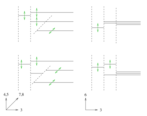
Figure 11: Allowed brane motions for the 2 solution branches of the D5-D5-D5^′ configuration. The top configuration has 5 adjustable parameters and the bottom has six, shown by green arrows.

D5-D5^′-D5

In the $U(2)$ region we have

$$\mathcal{X} = \left(\begin{array}[]{cc}a&0\\ 0&0\end{array}\right)\ ,$$ (4.51)

$$\mathcal{Y} = \left(\begin{array}[]{cc}0&b\\ c&d\end{array}\right)\ .$$ (4.54)

Crossing the D5 brane on the right, we have

$$\mathcal{X} = \left(\begin{array}[]{ccc}a&0&r\\ 0&0&s\\ u&v&t\end{array}\right)\ ,$$ (4.58)

$$\mathcal{Y} = \left(\begin{array}[]{ccc}0&b&0\\ c&d&0\\ 0&0&0\end{array}\right)\ .$$ (4.62)

The commutation relation $[\mathcal{X},\mathcal{Y}]=0$ implies

$$\left(\begin{array}[]{ccc}&ba&-bs\\ -ca&0&-cr-sd\\ cv&bu+vd&0\end{array}\right)=0\ .$$ (4.66)

There are various branches. One involves setting $b=c=v=s=0$ giving rise to a five dimensional branch parameterized by $a$, $d$, $u$, $r$, and $t$, illustrated in figure 12 on top. Another involves setting $a=r=s=u=v=0$ giving rise to a four dimensional branch parameterized by $b$, $c$, $d$, and $t$, illustrated in figure 12 on bottom.

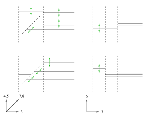
Figure 12: Brane configuration for the 2 solution branches of the D5-D5^′-D5 configuration. The top configuration has five adjustable parameters and the bottom has four, shown by green arrows.

D5^′-D5-D5

This is the easiest case for $U(3)$. One component of $\mathcal{X}$ is fixed to a fiducial value, while for the rest of the components we have

$$\mathcal{X} = \left(\begin{array}[]{ccc}0&b&c\\ d&e&f\\ g&h&j\end{array}\right)\ ,$$ (4.70)

$$\mathcal{Y} = \left(\begin{array}[]{ccc}a&&\\ &0&\\ &&0\end{array}\right).$$ (4.74)

If $a\neq 0$, we are forced to set $b=c=d=g=0$, and so we have a five dimensional space parameterized by $a$, $e$, $f$, $h$, and $j$. If $a=0$, there are no additional constraints on $\mathcal{X}$ and so it is parameterized by eight variables $b$, $c$, $d$, $e$, $f$, $g$, $h$, and $j$. The brane configuration associated with these deformation is illustrated in figure 13.

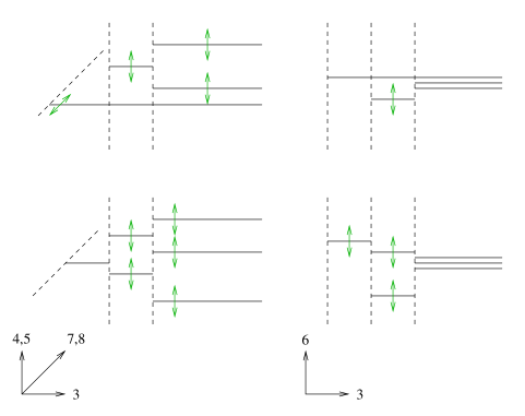
Figure 13: Brane configurations for the 2 branches of the D5^′-D5-D5 system. The top configuration with $a\neq 0$ has five adjustable parameters and the bottom with $a=0$ has eight, indicated by green arrows.

4.2.3 1/4 BPS Pole Boundary Conditions

When we allow both D5 and D5^′ branes we can also have 1/4 BPS configurations with poles, as shown in figure 14.

Figure 14: 1/4 BPS $U(3)$ boundary conditions with poles.

We want to generalize the procedure for handling poles to 1/4 BPS. There are a few subtle points. We will now have two matrices $\mathcal{X}$ and $\mathcal{Y}$. Therefore we have to impose singularity constraints on both of them. We will also have to be careful in modding out by residual gauge transformations, which will act on both $\mathcal{X}$ and $\mathcal{Y}$.

First we consider case (a). We begin in the $U(2)$ region, $0<y<y_{1}$, where $y_{1}$ is the position of D5^′ in the $y$-direction. According to our rules for treating D5 and and D5^′ boundary conditions, we should set $\mathcal{Y}=0$. We also have

$$\mathcal{A}=\frac{1}{2y}\left(\begin{array}[]{ccc}1&0&0\\ 0&-1&0\\ 0&0&0\end{array}\right)\ ,$$ (4.78)

so that we will solve all the constraints in the $U(2)$ region with

$$\mathcal{X} = \left(\begin{array}[]{ccc}a&1/y&\\ by&a&\\ &&\end{array}\right)\ ,$$ (4.82)

$$\mathcal{Y} = \left(\begin{array}[]{ccc}0&0&\\ 0&0&\\ &&\end{array}\right)\ .$$ (4.86)

Proceeding to the $U(3)$ region, $y>y_{1}$, we should put zeros in $\mathcal{X}$ off the diagonal while $\mathcal{Y}$ grows in all of the new entries; at the boundary we may choose any values for these entries but they also have a $y$ dependence given by the complex equation $\mathcal{D}\mathcal{Y}=0$:

$$\mathcal{X} = \left(\begin{array}[]{ccc}a&1/y&0\\ by&a&0\\ 0&0&0\end{array}\right)\ ,$$ (4.90)

$$\mathcal{Y} = \left(\begin{array}[]{ccc}0&0&uy^{-1/2}\\ 0&0&vy^{1/2}\\ ry^{1/2}&sy^{-1/2}&t\end{array}\right)\ .$$ (4.94)

Of course the $y^{-1/2}$ terms are nonsingular because they are defined only for $y\geq y_{1}>0$.

We are not done because we still have to impose the 1/4 BPS commutator equation $[\mathcal{X},\mathcal{Y}]=0$. This gives the equations

$$au+v = 0\ ,$$ (4.95)

$$av+bu = 0\ ,$$ (4.96)

$$ar+bs = 0\ ,$$ (4.97)

$$as+r = 0\ .$$ (4.98)

This system of equations has solutions when

$$b=a^{2}\ ,$$ (4.99)

with $u$ determined by $v$ and $r$ determined by $s$. In this case the configurations are parameterized by four variables, $a$, $v$, $s$, and $t$. The other possiblity is for $a=b=0$ which also forces $r=v=0$ giving rise to a three parameter branch of solutions parameterized by $u$, $s$, and $t$, which we illustrate in figure 15.

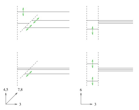
Figure 15: Allowed brane motions for the two branches associated with the configuration of figure 14.a. The top configuration has four adjustable parameters and the bottom with has three, indicated by green arrows.

Note that on this branch, if we try to take the limit $y_{1}\rightarrow 0$ we encounter singular terms proportional to $y^{-1/2}$. (For finite brane separations, this is not singular because it is evaluated at $y_{1}$.) In the 1/2 BPS analysis of [1], a similar singularity was found for the analogous brane configuration with only D5-branes. They pointed out that this configuration can be related to the 1/2 BPS version of figure 14 accompanied by some decoupled free sectors by changing the ordering of the branes, and argued that they are therefore redundant in their classification scheme. Since branes can not be reordered with similar control in the case with 1/4 BPS, and since the way in which decoupled sectors arise is generally more intricate [23, 24], it seems less convincing to attribute the singularity here as a signature of some free decoupled sector.

Another noteworthy feature of the three dimensional branch illustrated on the bottom of figure 15 is the fact that the positions of three semi-infinite D3’s along the ${\cal Y}=X_{7}+iX_{8}$ coordinates are not the most general ones allowed from the consideration of the brane configurations. In fact, only one of the three semi-infinite D3-branes are allowed to move in the ${\cal Y}$ direction. This is one of the manifestations of the non-abelian dynamics which we will explore in greater detail in the follow up paper [9].

Next we consider case (b). Here the pole is at $y=y_{1}$ and we set

$$\mathcal{A}=\frac{1}{2(y-y_{1})}\left(\begin{array}[]{ccc}1&0&0\\ 0&-1&0\\ 0&0&0\end{array}\right)\ .$$ (4.103)

We must also have (using our rules for crossing D5 and D5^′)

$$\mathcal{X}=\left(\begin{array}[]{ccc}0&0&0\\ 0&0&0\\ 0&0&a\end{array}\right)\ ,$$ (4.107)

(we have reversed the ordering of rows and columns) while $\mathcal{Y}$ has one element fixed at the boundary and one element fixed by the singularity structure:

$$\mathcal{Y}=\left(\begin{array}[]{ccc}0&(y-y_{1})^{-1}&\\ &0&\\ &&0\end{array}\right)\ ,$$ (4.111)

and the empty elements are still to be filled in. Solving the complex Nahm equation and modding out by $G_{C}$ requires

$$\mathcal{Y}=\left(\begin{array}[]{ccc}d&(y-y_{1})^{-1}&u(y-y_{1})^{-1/2}\\ e(y-y_{1})&d&v(y-y_{1})^{1/2}\\ r(y-y_{1})^{1/2}&s(y-y_{1})^{-1/2}&0\end{array}\right)\ .$$ (4.115)

We see that there are unwanted singular coefficients at $y=y_{1}$ off the diagonal. These have to be set to zero:

$$\mathcal{Y}=\left(\begin{array}[]{ccc}d&(y-y_{1})^{-1}&0\\ e(y-y_{1})&d&v(y-y_{1})^{1/2}\\ r(y-y_{1})^{1/2}&0&0\end{array}\right)\ ,$$ (4.119)

and we should impose $[\mathcal{X},\mathcal{Y}]=0$. There is a branch of configurations with $a=0$ and $d,e,r,v$ unconstrained, and another branch with $v=r=0$, and $a,d,e$ unconstrained.

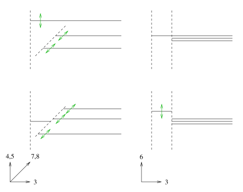
Figure 16: Allowed brane motions for the two branches associated with the brane configuration of figure 14.b. The top configuration has three adjustable parameters and the bottom with has four, indicated by green arrows.

This configuration does have a simple $y_{1}\rightarrow 0$ limit, because the boundary conditions forced us to drop the potentially singular terms.

4.3 $T[SU(N)]$ and Its 1/4 BPS Generalizations

In this subsection, we consider boundaries made out of NS5-branes in place of the D5-branes which appeared in the previous subsection. Typical boundaries which arise in this way are illustrated in figure 17. They are related to the analysis of the previous section by S-duality. We will first review the case where 1/2 of the supersymmetry is preserved, and then proceed to generalize to the 1/4 BPS case.

Figure 17: Basic configuration of the boundary theory generally referred to as $T(SU(N)$. Here, the case for $N=3$ is illustrated.

4.3.1 $T[SU(N)]$

We can understand the NS5/NS5^′ boundary condition in terms fo a coupling of the bulk $\mathcal{N}=4$ SYM theory to a boundary $\mathcal{N}=2$ theory via bifundamentals. Note that the bifundamental couplings can look different depending on whether the right-most boundary is NS5 or NS5^′ (unlike 3$d$ $\mathcal{N}=4$, the bifundamental coupling is not universal when only four supersymmetries are preserved.)

In the 1/2 BPS case, the Nahm pole boundary conditions ($N$ D3-branes ending on a D5) are S-dual to ordinary Neumann boundary conditions ($N$ D3-branes ending on NS5.) The ordinary Dirichlet boundary conditions, on the other hand, are S-dual to a coupling to a quiver gauge theory which GW called $T[SU(N)]$, corresponding to $N$ D3-branes ending on $N$ NS5-branes. It is not hard to see that coupling to $T[SU(N)]$ fixes the characteristic polynomial of $\mathcal{X}$.

NS5-NS5

Let us revisit coupling to $T[SU(2)]$. The brane configuration is NS5—1D3(1)—NS5—2D3(2)—(semi-infinite). See also figure 18. We will assume that generic complex FI terms are turned on. Note that when we couple this boundary condition to some configuration on the right there can be a $U(2)$ gauge transformation relating the two conditions.

From the first NS5, we have

$$\mathcal{X}_{1}=-\zeta_{1}\ ,\qquad\mathcal{Y}_{1}=a\ ,$$ (4.120)

and at the 1-2 interface we find

$$\mathcal{X}_{1} = A_{1}B_{1}-\zeta_{2}\ ,$$ (4.121)

$$\mathcal{X}_{2} = B_{1}A_{1}-\zeta_{2}\left(\begin{array}[]{cc}1&0\\ 0&1\end{array}\right)\ .$$ (4.124)

$A_{1}$ is a row vector and $B_{1}$ is a column vector in this example. This sets

$$\mathcal{X}_{2} = \left(\begin{array}[]{cc}-\zeta_{1}&0\\ 0&-\zeta_{2}\end{array}\right)\ ,$$ (4.127)

$$\mathcal{Y}_{2} = \left(\begin{array}[]{cc}a&0\\ 0&b\end{array}\right)\ ,$$ (4.130)

$$A_{1} = (\zeta_{2}-\zeta_{1},0)\ ,$$ (4.131)

$$B_{1} = \left(\begin{array}[]{c}1\\ 0\end{array}\right)\ ,$$ (4.134)

up to a gauge transformation, provided that $\zeta_{1}\neq\zeta_{2}$. There are two parameters, $a$ and $b$. This configuration and the geometric interpretation of the two parameters is illustrated in figure 18.a.

If, instead, the two FI parameters take equal values, then we can have

$$\mathcal{X}_{2} = \left(\begin{array}[]{cc}-\zeta_{1}&1\\ 0&-\zeta_{1}\end{array}\right)\ ,$$ (4.137)

$$\mathcal{Y}_{2} = \left(\begin{array}[]{cc}a&b\\ 0&a\end{array}\right)\ ,$$ (4.140)

$$A_{1} = (0,1)\ ,$$ (4.141)

$$B_{1} = \left(\begin{array}[]{c}1\\ 0\end{array}\right)\ .$$ (4.144)

Here, the form of the matter fields introduces an off-diagonal element in (4.137); this possibility is consistent with the fact that when two or more eigenvalues of a matrix coincide one cannot always diagonalize the matrix, but it can always be put in the upper triangular Jordan normal form. Once again, we find two parameters, $a$, and $b$, but their physical interpretation, illustrated in figure 18.b, is different. The parameter $b$ does not affect the eigenvalues of $\cal X$ or $\cal Y$ and as such does not deform the branes geometrically in these directions. Instead, it encodes aspects of the embedding in the $X_{6}$ coordinate which requires additional care. In addition, having this parameter non-vanishing binds the finite D3 segment and the two semi-infinite D3 branes so the entire collection of D3-branes move together. This is one of the novel features of the $T[SU(2)]$ not previously seen in the S-dual configuration built using the D5-branes. It should also be viewed as a subtle consequence of S-duality being non-local. We will elaborate further on this point below.

Another possible branch arises from the case

$$\mathcal{X}_{2} = \left(\begin{array}[]{cc}-\zeta_{1}&0\\ 0&-\zeta_{1}\end{array}\right)\ ,$$ (4.147)

$$\mathcal{Y}_{2} = \left(\begin{array}[]{cc}a&0\\ 0&a\end{array}\right)\ ,$$ (4.150)

$$A_{1} = (0,b)\ ,$$ (4.151)

$$B_{1} = \left(\begin{array}[]{c}0\\ 0\end{array}\right)\ ,$$ (4.154)

whose geometric interpretation also involves the deformation of the semi-infinite D3 in the $X_{6}$ direction (there is a potential issue with stability of the complex gauge quotient for this branch, which will be described in detail in [9].) For now we will illustrate it as figure 18.c. There will be another closely related branch with non-vanishing $B_{1}$ and $A_{1}=0$.

Finally, if we set $\zeta_{1}=\zeta_{2}$ without including the Jordan form terms, there will be an unbroken gauge symmetry which we illustrate in figure 18.d. It is the branches (a) and (d) which has immediate counterparts in the S-dual. However, since (d) leaves some gauge symmetry unbroken, and involves turning on $X_{9}$, we expect the classical picture to receive corrections. The fact that we have access to enumerating boundary deformation classically in one description and the S-dual will eventually enable us to infer the self-consistent quantum corrected description of the moduli space when these boundaries are used to define a system on a finite interval, which we will explore in detail in [9].

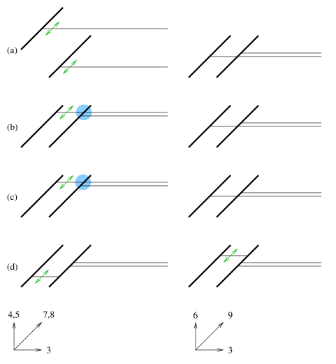
Figure 18: Brane configuration for $T[SU(2)]$ with distinct FI terms, and three case with coincident FI terms. The blue disk indicates one complex degree of freedom associated with a deformation localized at the defect which does not deform the branes geometrically in ${\cal X}$ and ${\cal Y}$ directions, but in some cases may affect the $X_{6}$ embedding (not drawn in figure). The blue disk also has the effect of forcing the D3 interval and two semi infinite D3 branes to bind and move collectively in the ${\cal Y}$ direction as indicated by the green arrows in (b) and (c). For the case illustrated in (d), there will be an unbroken $U(1)$ gauge symmetry giving rise to a two complex dimensional moduli from the ${\cal N}=4$ vector multiplet illustrated using the green arrows.

This structure generalizes to $T[SU(N)]$. We will have that $\mathcal{X}_{N}$ is a matrix in Jordan normal form. $\mathcal{Y}_{N}$ will then be forced to be a commuting matrix, also in Jordan normal form, except that we do not have enough gauge freedom to set the off-diagonal elements to 1.

4.3.2 1/4 BPS Generalization of $T[SU(N)]$

NS-NS^′

Now suppose we rotate the second NS5 to NS5^′. Then we have

$$\mathcal{Y}_{1} = A_{1}B_{1}-\zeta_{2}=a\ ,$$ (4.155)

$$\mathcal{Y}_{2} = B_{1}A_{1}-\zeta_{2}\left(\begin{array}[]{cc}1&0\\ 0&1\end{array}\right)\ .$$ (4.158)

This implies that up to a gauge transformation we must be able to have

$$\mathcal{Y}_{2} = \left(\begin{array}[]{cc}a&0\\ 0&-\zeta_{2}\end{array}\right)\ ,$$ (4.161)

$$\mathcal{X}_{2} = \left(\begin{array}[]{cc}-\zeta_{1}&0\\ 0&b\end{array}\right)\ ,$$ (4.164)

and gives rise to a branch with two degrees of freedom, $a$, and $b$, illustrated in figure 19.a. There is a special case when $a=-\zeta_{2}$ and $b=-\zeta_{1}$. Then we can have a one complex dimensional branch parameterized by $c$

$$\mathcal{Y}_{2} = \left(\begin{array}[]{cc}-\zeta_{2}&1\\ 0&-\zeta_{2}\end{array}\right)\ ,$$ (4.167)

$$\mathcal{X}_{2} = \left(\begin{array}[]{cc}-\zeta_{1}&c\\ 0&-\zeta_{1}\end{array}\right)\ ,$$ (4.170)

illustrated in figure 19.b. There is also a branch where ${\cal X}$ will not be in the Jordan normal form, for which the gauge symmetry is not broken. The brane configuration for that branch is illustrated in figure 19.c up to gauge transformations. Note also that the freedom to one of the semi-infinite D3 freely in the ${\cal X}$ direction is not captured in this branch.

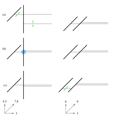
Figure 19: Brane configuration for NS5–D3–NS5^′–2D3–. This is the S-dual of configuration illustrated in figure 9. Unlike in the case of figure 9, some data pertaining to the embedding in the $X_{6}$ direction such as the real component of the FI parameter is contained in the blue disk in (b).

How does this generalize to $N$ 5-branes? It appears that in this case, for each NS5 or NS5^′, one eigenvalue of $\mathcal{X}_{N}$ or $\mathcal{Y}_{N}$, respectively, is fixed by the FI parameter of that 5-brane, while correspondingly one gets a meson in $\mathcal{Y}_{N}$ or $\mathcal{X}_{N}$. When some of the eigenvalues coincide one can only put the matrix in Jordan normal form, and then there is only enough freedom to set the off-diagonal elements to 1 in either $\mathcal{X}$ or $\mathcal{Y}$ but not both.

NS5-NS5-NS5

Let us write it out explicitly for $T[SU(3)]$. We will find

$$\mathcal{X}_{3} = \left(\begin{array}[]{ccc}-\zeta_{1}&&\\ &-\zeta_{2}&\\ &&-\zeta_{3}\end{array}\right)\ ,$$ (4.174)

$$\mathcal{Y}_{3} = \left(\begin{array}[]{ccc}\;\;a&&\\ &\;\;b&\\ &&\;\;c\end{array}\right)\ ,$$ (4.178)

unless some of the $\zeta_{i}$ are equal. If two are equal, then we also have to consider

$$\mathcal{X}_{3} = \left(\begin{array}[]{ccc}-\zeta_{1}&&\\ &-\zeta_{2}&1\\ &&-\zeta_{2}\end{array}\right)\ ,$$ (4.182)

$$\mathcal{Y}_{3} = \left(\begin{array}[]{ccc}\;\;a&&\\ &\;\;b&\;\;c\\ &&\;\;b\end{array}\right)\ .$$ (4.186)

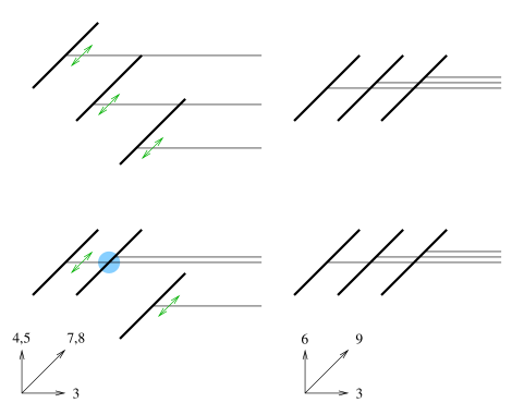
Figure 20: Brane configuration for NS5–D3–NS5–2D3–NS5–3D3–.

The three parameters $a$, $b$, and $c$ in (4.174)–(4.178) and (4.182)–(4.186) are represented by green arrows and blue disks in figure 20.

NS5-NS5-NS5^′

If we have two NS5 and one NS5^′, we should write

$$\mathcal{X}_{3} = \left(\begin{array}[]{ccc}-\zeta_{1}&&\\ &-\zeta_{2}&\\ &&c\end{array}\right)\ ,$$ (4.190)

$$\mathcal{Y}_{3} = \left(\begin{array}[]{ccc}\;\;a&&\\ &\;\;b&\\ &&-\zeta_{3}\end{array}\right)\ ,$$ (4.194)

assuming the eigenvalues are all distinct. The three parameteres $a$, $b$, and $c$ in (4.190)–(4.194) corresponds to the green arrows and blue disks in figure 21.

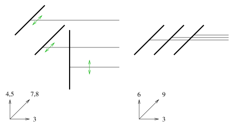
Figure 21: Brane configuration for NS5–D3–NS5–2D3–NS5^′–3D3–.

It should be clear now that we can prove our statement about the structure of the boundary conditions for general $N$ by the method of induction. We assume the form of the boundary condition for $T[SU(N-1)]$ (that is, $N-1$ NS5-branes with one D3-brane ending on each NS5), so $\mathcal{X}_{N-1}$ and $\mathcal{Y}_{N-1}$ are some $(N-1)\times(N-1)$ diagonal matrices (if the eigenvalues are distinct.) Then we couple it to an NS5 brane (or NS5^′) with the $N-1$ D3-branes on one side and $N$ D3-branes on the other. We then have (for NS5)

$$\mathcal{X}_{N-1} = AB-\zeta I_{N-1}\ ,$$ (4.195)

$$\mathcal{X}_{N} = BA-\zeta I_{N}\ .$$ (4.196)

We need to determine the eigenvalues of $\mathcal{X}_{N}$ in terms of those for $\mathcal{X}_{N-1}$. This can be done easily as follows. Suppose $v$ is an eigenvector of $\mathcal{X}_{N-1}$, with

$$\mathcal{X}_{N-1}v=\lambda v\ .$$ (4.197)

As long as $Bv\neq 0$, one then checks that $Bv$ is an eigenvector of $\mathcal{X}_{N-1}$ with eigenvalue $\lambda$. If the gauge symmetry is unbroken, one can always find $N-1$ such eigenvectors, either as column eigenvectors $v$ in which case we multiply to form $Bv$ or row eigenvectors $u$ and we construct $uA$. So $N-1$ of the eigenvalues of $\mathcal{X}_{N}$ are equal to the eigenvalues of $\mathcal{X}_{N-1}$. To fix the last eigenvalue, we compute

$${\rm Tr}(\mathcal{X}_{N})-{\rm Tr}(\mathcal{X}_{N-1})={\rm Tr}(BA-\zeta I_{N})-{\rm Tr}(AB-\zeta I_{N-1})=-\zeta\ ,$$ (4.198)

so the $N$-th eigenvalue of $\mathcal{X}_{N}$ is $-\zeta$.

Now we need to fix the eigenvalues of $\mathcal{Y}_{N}$ in terms of the eigenvalues of $\mathcal{Y}_{N-1}$. We use

$$B\mathcal{Y}_{N-1}=\mathcal{Y}_{N}B\ ,$$ (4.199)

and once again, we see that if $v$ is an eigenvector of $\mathcal{Y}_{N-1}$ with eigenvalue $\lambda$, $Bv$ is an eigenvector of $\mathcal{Y}_{N}$ with eigenvalue $\lambda$. This allows us to fix $N-1$ eigenvalues of $\mathcal{Y}_{N}$, provided that the gauge symmetry is fully broken. The $N$-th eigenvalue of $\mathcal{Y}_{N}$ is unfixed and free to vary. Note that each eigenvalue of $\mathcal{X}$ which is fixed by an FI term is paired with a free eigenvalue of $\mathcal{Y}$, and vice versa.

Because $[\mathcal{X},\mathcal{Y}]=0$, we can simultaneously diagonalize $\mathcal{X}_{N}$ and $\mathcal{Y}_{N}$. Note that this assumes that we have a $U(N)$ gauge symmetry to the right of the last NS5-brane. If the gauge symmetry is broken by the boundary conditions at infinity, then we can only impose the $T[SU(N)]$ boundary conditions up to a $GL(N)$ rotation.

If some of the eigenvalues are equal then we have to consider the corresponding Jordan normal forms as well. In fact, one can easily see that if we assume that $\mathcal{X}$ and $\mathcal{Y}$ are purely diagonal with mutually degenerate eigenvalues, the interface matter fields preserve some amount of unbroken gauge symmetry. Demanding that this gauge symmetry is broken forces us to only consider Jordan normal form.

5 Summary and Discussion

Let us pause and summarize the status of this paper. Our primary goal was to explore the boundary conditions which one can impose on ${\cal N}=4$ SYM in 3+1 dimensions such that the boundary preserves 1/4 of the supersymmetries, generalizing the earlier analysis for the case where 1/2 of the supersymmetries were preserved [1, 2].

Just as in the earlier work, we found that

1. A large class of boundaries can be constructed starting with the D3-brane intersecting with and terminating on NS5 and D5-branes arranged to preserve the correct number of supersymmetries.

2. The boundaries are equipped with parameters which can be viewed as deformation parameters, and unfixed degrees of freedom which can give rise to moduli of the theory at low energies.

3. For a given boundary, there exists a notion of the S-dual inherited from the S-duality of type IIB string theory.

In this article, we generalized the results of [1, 2] by including a broader class of orientations of the NS5 and D5-branes consistent with the reduced number of supersymmetries.

The main technical results which form the basis of our subsequent analysis are

• Generalized Nahm equations (3.6)–(3.9),

• Junction condition for D5 (3.37)–(3.40) and for D5^′ (3.51)–(3.54),

• Junction condition for NS5 (3.70)–(3.75) and for NS5^′ (3.76)–(3.81).

The analysis of the boundary conditions amounts to solving these sets of equations which are a combination of algebraic and first order differential relations.

As a practical tool to analyze the supersymmetry equations, it is convenient to employ the complex gauge formalism where the Nahm equation and the junction conditions are separated into complex equations and the real equations. This typically breaks the analysis into to two parts, where the complex part can be treated separately. Most of the interesting features are already contained in the analysis of the complex equations, without reference to the real equations. However there are situations (primarily related to real mass or FI deformations) where some important additional information relies on the analysis of the real part.

What we find from these analyses is that in many cases, the parameters characterizing the boundary correspond to moving brane segments around in the Hanany-Witten like picture (corresponding to the case where the fields are in some sense nearly Abelian and the notion of positions is well-defined.) However, when the fields have some intrinsically non-Abelian structure, there are some departures from the naive expectations based on brane diagrams alone. This is to be expected since one expects more quantum corrections with few preserved supersymmetries. It is, after all, well known that there are more quantum corrections to ${\cal N}=2$ supersymmetric gauge theories in 2+1 dimensions compared to ${\cal N}=4$ which can dynamically generate superpotentials and lift various branches of moduli space [20, 25, 5].

Some of the key departures and subtleties identified from our analysis are as follows.

1. Embedding of the semi-infinite bulk in the $X_{6}$ coordinate is hidden as is illustrated in figure 9. This feature is also shared by the 1/2 BPS constructions of [1, 2] but was not emphasized in their treatment.

2. Some configurations which are naively allowed from the consideration of naive Hanany-Witten brane constructions are not realized in the Nahm analysis. An example of this is illustrated in figure 15 in section 4.2.3 where only one of the three deformations of the semi-infinite D3 segments are allowed to move in the ${\cal Y}=X_{7}+iX_{8}$ directions. This is an example of lifting of branches naively expected from brane considerations.

3. There are degrees of freedom, illustrated in figures 18, 19, and 20 which do not have any geometric interpretation as movement in the ${\cal X}=X_{4}+iX_{5}$, ${\cal Y}=X_{7}+iX_{8}$, or $X_{9}$ directions. We will see in a followup paper [9] that these deformations have a role in adjusting the $X_{6}$ coordinates. This further illustrates the subtleties involving the embedding in the $X_{6}$ coordinate.

4. Another feature, noted in section 4.2.3, is the fact that the limit of coincident D5 and D5^′ branes is singular depending on the direction in which this limit is approached. This is in contrast to the half BPS cases where the positions of the 5-branes are irrelevant in the infrared. One important consequence of this observation is the fact that the classification of 1/4 BPS boundaries along the lines of GW’s treatment [1, 2] based on the decoupling of 5-brane positions does not immediately generalize.

It appears though that generally, these boundaries have parameters characterizing deformations consistent with the supersymmetry constraints (3.6)–(3.9), (3.37)–(3.40), (3.51)–(3.54), (3.70)–(3.75), and (3.76)–(3.81).

An important question one must address is whether these constraints derived at the classical level receive quantum corrections. Generally, one expects a variety of perturbative and non-perturbative corrections for dynamics of 2+1 dimensional systems with ${\cal N}=2$ supersymmetry [20, 25, 5, 6]. These boundary systems have the same amount of isometries and supersymmetries, so we should expect similar corrections.

A powerful tool to assess the role of quantum corrections is S-duality. Through S-duality, a model in the weak coupling limit probes the strong coupling limit of the S-dual theory. Using S-duality, one can therefore access the theory in two opposing limits. By identifying features such as the dimension of space of variables parameterizing the boundaries, one can assess if any of these features are likely to be constant with respect to the change in coupling and therefore protected against quantum corrections.

Furthermore, one can argue that if the gauge symmetry is completely broken in one of the duality frames, the supersymmetry constraints (3.6)–(3.9), (3.37)–(3.40), (3.51)–(3.54), (3.70)–(3.75), and (3.76)–(3.81) are protected against certain corrections (such as instanton corrections.) Using these ingredients, one can attempt to patch together a self-consistent picture of the complex structure of the parameter space which takes quantum corrections into account.

We have considered the simplest 1/4 BPS boundary consisting of D5 and D5^′ branes illustrated in figure 9 and its S-dual illustrated in figure 19. We in fact see that under S-duality, branch (a) of figure 9 is naturally mapped to branch (a) of figure 19 in the S-dual. Similarly, branch (b) of figure 9 appears to correspond to branch (c) of figure 19. For this branch, we see that there are unbroken gauge symmetries in the latter description, so we take the former to be the more reliable description.

The status of branch (b) in figure19 is somewhat curious. There is no counterpart of this branch in figure 9. Nonetheless, gauge symmetry is completely broken in the duality frame depicted by figure 19 and as such one expects this branch to be reliable. So why does it not show up in the figure 9 frame?

The answer to this question has to do with the subtlety of the treatment of the $X_{6}$ coordinate as well as the accounting of the boundary condition infinitely far away in the $X_{3}$ direction. The point is that the bulk scalar fields need to be specified at infinity in order to define the moduli space rigorously. In addition, in comparing the moduli spaces of two different S-dual descriptions of the same system, it is necessary to properly S-dualize the boundary condition at infinity consistently. In particular, because S-duality is strictly not a local transformation in space-time, some features specifying the boundary condition at infinity on one end in one duality frame might map to some features localized near the other boundary.

One way to systematically resolve these issues is to carefully construct the system on an interval terminated by boundary conditions on both ends, and to compare the moduli space on both sides. Such a construction is precisely the prescription to engineer ${\cal N}=2$ field theories in 2+1 dimensions along the line illustrated in figure 5. Taking advantage of S-duality and protection against potential quantum correction in cases where gauge symmetry is completely broken, we should be able to piece together the complicated branching structure of moduli spaces of field theories in 2+1 dimensions with 4 supercharges. Some of these issues have been studied previously using tools such as brane construction, mirror symmetry, and some inspired guesswork [20, 25, 5]. The 1/4 BPS conditions (3.6)–(3.9), (3.37)–(3.40), (3.51)–(3.54), (3.70)–(3.75), and (3.76)–(3.81) turns out to offer a new systematic approach to analyze these issues and offer some new insights. We will report on our findings on these matters in part II of this paper [9].

Appendix A Analysis of BPS Boundary Conditions

A.1 Spinor Algebra

To perform explicit computations with the fermions, it is often useful to have an explicit basis for the $\Gamma$-matrices which realizes the global symmetries of the system of interest in a natural way. For boundaries with $\mathcal{N}=4$ supersymmetry, we have the global symmetry ${SO(2,1)}\times{SO(3)}\times{SO(3)}$ which acts naturally on the 012, 456, 789 directions. For our purposes, a convenient basis may be defined as follows:

$${\Gamma_{0}} = \;{i\sigma_{2}}\otimes 1\otimes 1\otimes 1\otimes\sigma_{2}\ ,$$ (A.1)

$${\Gamma_{1}} = \;{\sigma_{1}}\otimes 1\otimes 1\otimes 1\otimes\sigma_{2}\ ,$$ (A.2)

$${\Gamma_{2}} = \;{\sigma_{3}}\otimes 1\otimes 1\otimes 1\otimes\sigma_{2}\ ,$$ (A.3)

$$\Gamma_{3} = \;\;1\otimes 1\otimes 1\otimes\sigma_{2}\otimes\sigma_{1}\ ,$$ (A.4)

$${\Gamma_{4}} = -1\otimes{\sigma_{1}}\otimes 1\otimes\sigma_{3}\otimes\sigma_{1}\ ,$$ (A.5)

$${\Gamma_{5}} = -1\otimes{\sigma_{2}}\otimes 1\otimes\sigma_{3}\otimes\sigma_{1}\ ,$$ (A.6)

$${\Gamma_{6}} = -1\otimes{\sigma_{3}}\otimes 1\otimes\sigma_{3}\otimes\sigma_{1}\ ,$$ (A.7)

$${\Gamma_{7}} = \;\;1\otimes 1\otimes{\sigma_{1}}\otimes\sigma_{1}\otimes\sigma_{1}\ ,$$ (A.8)

$${\Gamma_{8}} = \;\;1\otimes 1\otimes{\sigma_{2}}\otimes\sigma_{1}\otimes\sigma_{1}\ ,$$ (A.9)

$${\Gamma_{9}} = \;\;1\otimes 1\otimes{\sigma_{3}}\otimes\sigma_{1}\otimes\sigma_{1}\ ,$$ (A.10)

from which we compute

$${B_{0}} = \Gamma_{456789}=1\otimes 1\otimes 1\otimes{i\sigma_{2}}\otimes 1\ ,$$ (A.11)

$${B_{1}} = \Gamma_{3456}=1\otimes 1\otimes 1\otimes{\sigma_{1}}\otimes 1\ ,$$ (A.12)

$${B_{2}} = \Gamma_{3789}=1\otimes 1\otimes 1\otimes{\sigma_{3}}\otimes 1\ ,$$ (A.13)

$${\Gamma_{11}} = \bar{\Gamma}=1\otimes 1\otimes 1\otimes 1\otimes{\sigma_{3}}\ .$$ (A.14)

The convenience of this basis lies in the fact that the global symmetry ${SO(2,1)}\times{SO(3)}\times{SO(3)}$ acts simply on the first three entries of this tensor basis, the fourth entry transforms under an $SL(2,\mathbb{R})$ algebra (with generators $B_{0},B_{1},B_{2}$), and the fifth entry labels the 10-d chirality. The 16 component spinor $\epsilon_{L}$ of 4$d$ $\mathcal{N}=4$ is in representation $({\bf 2},{\bf 2},{\bf 2},{\bf 2})$.

There is also a Majorana condition which we should impose on the 10-d spinor, but it only fixes the phase multiplying the components of the spinors. In our analysis, this phase plays no role, but to be explicit, a possible Majorana condition is

$$\zeta^{*}=\Gamma_{4679}\zeta\ .$$ (A.15)

A.2 Half BPS Boundary Conditions

Let us first discuss the half BPS case, and analyze the boundary supersymmetry condition (2.5). Since we are interested in boundary conditions which preserve the $SO(2,1)\times SO(3)\times SO(3)$ global symmetry, we should not fix the spinors $\Psi$ and $\varepsilon$ in the the first three tensor indices of the basis in appendix A.1; also the Weyl condition fixes the fifth index. Therefore we fix half the components of $\Psi$ at the boundary by fixing the fourth spinor index. Specifically, in $\Psi$ and $\varepsilon$ we label the fourth spinor as ${\varepsilon_{0}}$ and ${\vartheta}$ (with arbitrary $v$ and $\psi$ labeling the first three spinor indices)

$$\varepsilon=v\otimes{\varepsilon_{0}}\ ,\qquad\Psi=\psi\otimes{\vartheta}\ .$$ (A.16)

Now, we expand $({\bf 2},{\bf 2},{\bf 2})$ components of $F\!\!\!\!/$

$${1\over 2}\Gamma\cdot F = ({\sigma_{\mu}},{1},{1}){R^{\mu}}+({\sigma_{\mu}},{\sigma_{a}},{1}){U_{\mu a}}+({\sigma_{\mu}},{1},{\sigma_{m}}){V_{\mu m}}$$ (A.18)

$$+({1},{\sigma_{a}},{1}){S_{a}}+({1},{1},{\sigma_{m}}){T_{m}}+({1},{\sigma_{a}},{\sigma_{m}}){W_{am}}\ .$$

The condition that half the supersymmetry is preserved is then simply that all the components in this tensor decomposition of $F\!\!\!\!/$ vanish: ${R^{\mu}}={U_{\mu a}}={V_{\mu m}}={S_{a}}={T_{m}}={W_{am}}=0$ with

$$\begin{split}R^{\mu}&=\epsilon^{\mu\nu\lambda}F_{\nu\lambda}({\bar{\varepsilon}_{0}\vartheta})+2F^{3\mu}({\bar{\varepsilon}_{0}B_{0}\vartheta})\ ,\cr U_{\mu a}&=2iD_{\mu}X_{a}({\bar{\varepsilon}_{0}B_{2}\vartheta})\ ,\cr V_{\mu m}&=-2iD_{\mu}Y_{m}({\bar{\varepsilon}_{0}B_{1}\vartheta})\ ,\cr W_{am}&=2[X_{a},Y_{m}]({\bar{\varepsilon}_{0}B_{0}\vartheta})\ ,\cr S_{a}&=2i[X_{b},X_{c}]\epsilon_{abc}({\bar{\varepsilon}_{0}\vartheta})-2iD_{3}X_{a}({\bar{\varepsilon}_{0}B_{1}\vartheta})\ ,\cr T_{m}&=2i[Y_{n},Y_{p}]\epsilon_{mnp}({\bar{\varepsilon}_{0}\vartheta})-2iD_{3}Y_{m}({\bar{\varepsilon}_{0}B_{2}\vartheta})\ ,\cr{B_{0}}&=i\sigma_{2}\ ,\cr{B_{1}}&=\sigma_{1}\ ,\cr{B_{2}}&=\sigma_{3}\ .\end{split}$$ (A.19)

To proceed further, we look for ${\varepsilon_{0}}$ and ${\vartheta}$ for which we can consistently solve this set of equations. First, in order to preserve the $SO(3)\times SO(3)$ R-symmetry, we have to impose the same set of boundary conditions for $X_{a}$ for $a=1,2,3$. The same applies to $Y_{a}$.

Up to an overall normalization we can write $\bar{\varepsilon}_{0}=(1,a),\vartheta=(\alpha,1)^{T}$ (we allow $a$ and $\alpha$ to be infinity.) We then have

$${\bar{\varepsilon}_{0}\vartheta}=a+\alpha\ ,\quad{\bar{\varepsilon}_{0}B_{0}\vartheta}=-a\alpha+1\ ,\quad{\bar{\varepsilon}_{0}B_{1}\vartheta}=a\alpha+1\ ,\quad{\bar{\varepsilon}_{0}B_{2}\vartheta}=\alpha-a\ .$$ (A.20)

Suppose first that both $X_{a}$ and $Y_{a}$ both obey Dirichlet boundary conditions. Then from the second and the third equations we have ${\bar{\varepsilon}_{0}B_{1}\vartheta}={\bar{\varepsilon}_{0}B_{2}\vartheta}=0$. This cannot be satisfied for real $\epsilon_{0}$ and $\vartheta$.

Suppose now that neither $X_{a}$ nor $Y_{a}$ obey Dirichlet boundary conditions. Then the fourth and the fifth equations tell us ${\bar{\varepsilon}_{0}B_{1}\vartheta}={\bar{\varepsilon}_{0}B_{2}\vartheta}=0$, which is again a contradiction.

If $X$ is Neumann and $Y$ is Dirichlet, we obtain

$$D_{3}X_{a}+{u\over 2}\epsilon_{abc}[X_{b},X_{c}]=0\ ,$$ (A.21)

with

$${0=\bar{\varepsilon}_{0}B_{2}\vartheta=\bar{\varepsilon}_{0}(1+uB_{1})\vartheta}\ .$$ (A.22)

We also have

$$\epsilon_{\lambda\mu\nu}F^{3\lambda}=\gamma F_{\mu\nu}\ ,$$ (A.23)

which implies

$${\bar{\varepsilon}_{0}(1+\gamma B_{0})\vartheta=0}\ .$$ (A.24)

This is solved by

$$\bar{\varepsilon}_{0}=(1,a)\ ,\qquad\vartheta=\left(\begin{array}[]{c}a\\ 1\end{array}\right)\ ,\qquad\gamma=-{2a\over 1-a^{2}}\ ,\qquad u=-{2a\over 1+a^{2}}\ .$$ (A.25)

Different choices of $a$ correspond to different types of boundary conditions, as discussed in the main text:

$\bullet\$$a=0$, $u=0$, $\gamma=0$: D3 ending on NS5 on ${012}{456}$

$\bullet\$$a=1$, $u=-1$, $\gamma=\infty$: D3 ending on D5 on ${012}{456}$

$\bullet\$$\gamma=-{g_{\rm YM4}^{2}\over 4\pi}{q\over p}$: D3 ending on $(p,q)5$ on ${012}{456}$

We can rotate these boundary conditions with the $SO(6)$ R-symmetry of the bulk, while preserving 1/2 BPS supersymmetry. For example, an NS5 on ${012}{456}$ and a D5 on ${012}{789}$ preserve the same eight supersymmetries. In the main text we mostly use these boundary conditions.

A.3 Rotated Branes

Our 4$d$ $\mathcal{N}=4$ $U(N)$ gauge theory is the low-energy effective theory on $N$ D3-branes extended along the 0123 directions. This preserves the supersymmetry

$$\epsilon_{L}=\Gamma_{0123}\,\epsilon_{R}\ .$$ (A.26)

If we add a D5-brane in $012345$, we have another constraint

$$\epsilon_{L}=\Gamma_{012456}\,\epsilon_{R}\ .$$

From (A.26), this is the same as

$$\epsilon_{L}=\,\Gamma_{3456}\,\epsilon_{L}\ ,\quad\epsilon_{R}=-\,\Gamma_{3456}\,\epsilon_{R}\ .$$ (A.27)

The total system consisting of D3 and D5 branes preserves 8 supercharges. Similarly, an NS5-brane in $0123456$-directions preserves

$$\epsilon_{L}=\Gamma_{012456}\,\epsilon_{L}\ ,\quad\epsilon_{R}=-\Gamma_{012456}\,\epsilon_{R}\ .$$

From the chirality constraint this is the same as

$$\epsilon_{L}=\Gamma_{3789}\,\epsilon_{L}\ ,\quad\epsilon_{R}=-\Gamma_{3789}\,\epsilon_{R}\ .$$ (A.28)

More generally, a $(p,q)$ 5-brane in $012[47]_{\psi}[58]_{\varphi}[69]_{\rho}$ preserves (under (A.26)) $\epsilon_{L},\epsilon_{R}$ satisfying

$$\epsilon_{L}=R_{\theta,\psi,\varphi,\rho}\Gamma_{3456}R_{\theta,\psi,\varphi,\rho}^{-1}\epsilon_{L}\ ,\quad\epsilon_{R}=-R_{\theta,\psi,\varphi,\rho}\Gamma_{3456}R_{\theta,\psi,\varphi,\rho}^{-1}\epsilon_{R}\ ,$$ (A.29)

or equivalently

$$(R_{\theta,\psi,\varphi,\rho}^{2}-1)\,\epsilon_{L}=\epsilon_{L},\quad(R_{\theta,\psi,\varphi,\rho}^{2}-1)\,\epsilon_{R}=\epsilon_{R}\ .$$ (A.30)

Here $\theta\equiv\pi\arctan\left(\frac{p}{q}\right)$, and the rotation matrix $R_{\theta,\psi,\varphi,\rho}$ given by

$$R_{\theta,\psi,\varphi,\rho}\equiv\exp\left(\frac{\theta}{2}\Gamma_{456789}+\frac{\psi}{2}\Gamma_{47}+\frac{\varphi}{2}\Gamma_{58}+\frac{\rho}{2}\Gamma_{69}\right)\ ,$$ (A.31)

whose square is computed to be

$$R_{\theta,\psi,\varphi,\rho}^{2}=\exp\left[1\otimes(\theta\,1\otimes 1+\psi\,\sigma_{1}\otimes\sigma_{1}+\varphi\,\sigma_{2}\otimes\sigma_{2}+\rho\,\sigma_{3}\otimes\sigma_{3})\otimes\sigma_{2}\otimes 1\right]\ .$$ (A.33)

Therefore (A.30) becomes the statement that the term inside the bracket, i.e.,

$$\theta\,1\otimes 1+\psi\,\sigma_{1}^{(2)}\otimes\sigma_{1}^{(3)}+\varphi\,\sigma_{2}^{(2)}\otimes\sigma_{2}^{(3)}+\rho\,\sigma_{3}^{(2)}\otimes\sigma_{3}^{(3)}\ ,$$ (A.34)

acts trivially on the second and the third components. The operator (A.34) has eigenvectors

$$\begin{aligned} |1\rangle&\equiv\frac{1}{\sqrt{2}}\left[|\!\!\uparrow\uparrow\rangle+|\!\!\downarrow\downarrow\rangle\right]\ ,\\ |2\rangle&\equiv\frac{1}{\sqrt{2}}\left[|\!\!\uparrow\uparrow\rangle-|\!\!\downarrow\downarrow\rangle\right]\ ,\\ |3\rangle&\equiv\frac{1}{\sqrt{2}}\left[|\!\!\uparrow\downarrow\rangle+|\!\!\downarrow\uparrow\rangle\right]\ ,\\ |4\rangle&\equiv\frac{1}{\sqrt{2}}\left[|\!\!\uparrow\downarrow\rangle-|\!\!\downarrow\uparrow\rangle\right]\ ,\end{aligned}$$ (A.35)

with eigenvalues

$$\begin{aligned} \theta_{1}&\equiv\theta+\rho+\psi-\varphi\ ,\\ \theta_{2}&\equiv\theta+\rho-\psi+\varphi\ ,\\ \theta_{3}&\equiv\theta-\rho+\psi+\varphi\ ,\\ \theta_{4}&\equiv\theta-\rho-\psi-\varphi\ .\end{aligned}$$ (A.36)

When the angles $\theta,\psi,\varphi,\rho$ are generic this means all the supersymmetries are broken. However, in special situations some of (A.36) are zero, and corresponding supersymmetry is preserved. This gives Table 1. Note that the number of unbroken symmetry is preserved under permutations of $\theta,\psi,\varphi,\rho$.

	condition	3$d$ SUSY	5-brane
I	all angles zero	$\mathcal{N}=4$	D5$\left(012456\right)$
II-1	$\theta=\psi=\varphi=-\rho$	$\mathcal{N}=3$	$(p,q)5\left(012\left[{4}\atop{7}\right]_{\theta}\left[{5}\atop{8}\right]_{\theta}\left[{6}\atop{9}\right]_{-\theta}\right)$
II-2	$-\theta=\psi=\varphi=\rho$		$(p,q)5\left(012\left[{4}\atop{7}\right]_{-\theta}\left[{5}\atop{8}\right]_{-\theta}\left[{6}\atop{9}\right]_{-\theta}\right)$
III-1	$\varphi=\psi,\rho=-\theta$	$\mathcal{N}=2$	$(p,q)5\left(012\left[{4}\atop{7}\right]_{\psi}\left[{5}\atop{8}\right]_{\psi}\left[{6}\atop{9}\right]_{-\theta}\right)$
III-2	$\theta=\rho=0,\psi=\varphi$		D5$\left(012\left[{4}\atop{7}\right]_{\psi}\left[{5}\atop{8}\right]_{\psi}6\right)$
III-3	$\psi=\varphi=0,\rho=\theta$		$(p,q)5\left(01245\left[{6}\atop{9}\right]_{\theta}\right)$
IV	$\rho=\theta+\psi+\varphi$	$\mathcal{N}=1$	$(p,q)5\left(012\left[{4}\atop{7}\right]_{\psi}\left[{5}\atop{8}\right]_{\varphi}\left[{6}\atop{9}\right]_{\theta+\psi+\varphi}\right)$

Table 1: The classification of supersymmetries preserved, when we have D3-D5(012456) and an extra 5-brane, where we defined $\theta=\pi\arctan\left(p/q\right)$. The number of remaining supersymmetries is determined simply from the number of zeros in the four angles (A.36). This is a reformat of the similar table from [35].

A.4 1/4 BPS Case

In this appendix we explore the 1/4 BPS boundary conditions in a framework more general than that of the main text, at least those corresponding to the 1/4 BPS case of (2.105). What is special about the brane configuration there is that the system has $SO(2)_{45}\times SO(2)_{78}$ symmetry, corresponding to the rotation symmetry of $45$ and $78$-planes; we expect that the general 3$d$ $\mathcal{N}=2$ theory to have only one $SO(2)$ symmetry, namely the R-symmetry of the theory.

As we learn from the analysis of the previous subsection, the supersymmetries preserved by the D3-D5-D5^′ system is spanned by $|1\rangle,|2\rangle$ (case III-2 in table 1). Motivated by this, we choose the Ansatz

$$\bar{\epsilon}^{T}=\{|1\rangle\otimes|\!\!\uparrow\rangle+a|1\rangle\otimes|\!\!\downarrow\rangle\ ,\quad|2\rangle\otimes|\!\!\uparrow\rangle+a|2\rangle\otimes|\!\!\downarrow\rangle\}\ ,$$ (A.37)

and

$$\begin{split}\Gamma_{3}\Psi\in\textrm{span}\Big{\{}&\beta|1\rangle\otimes|\!\!\uparrow\rangle+|1\rangle\otimes|\!\!\downarrow\rangle\ ,\qquad\beta|2\rangle\otimes|\!\!\uparrow\rangle+|2\rangle\otimes|\!\!\downarrow\rangle\ ,\\ &\alpha|3\rangle\otimes|\!\!\uparrow\rangle+|3\rangle\otimes|\!\!\downarrow\rangle\ ,\qquad\alpha|4\rangle\otimes|\!\!\uparrow\rangle+|4\rangle\otimes|\!\!\downarrow\rangle\Big{\}}\ .\end{split}$$ (A.38)

The one parameter $a$ (two parameters $\alpha,\beta$) determines the choice of two (four) out of ${\bf 2}\otimes{\bf 2}\otimes{\bf 2}$. Note that this Ansatz is consistent with the $SO(2)_{45}\times SO(2)_{78}$ symmetry, which mixes two states $|1\rangle$ and $|2\rangle$, and also states $|3\rangle$ and $|4\rangle$. The equation (2.5) simplify considerably under this Ansatz, and we obtain

$$cF_{\mu\nu}+c_{0}\,\epsilon_{\mu\nu\lambda}F_{3\lambda} =0\ ,$$ (A.39)

$$c_{1}D_{\mu}X_{9}-c_{2}D_{\mu}X_{6} =0\ ,$$ (A.40)

$$d_{2}D_{\mu}X_{4}=d_{2}D_{\mu}X_{5} =0\ ,$$ (A.41)

$$d_{1}D_{\mu}X_{7}=d_{1}D_{\mu}X_{8} =0\ ,$$ (A.42)

$$c_{0}[X_{6},X_{9}] =0\ ,$$ (A.43)

$$c_{0}([X_{5},X_{7}]+[X_{4},X_{8}]) =0\ ,$$ (A.44)

$$c_{0}([X_{5},X_{8}]-[X_{4},X_{7}]) =0\ ,$$ (A.45)

$$d_{1}D_{3}X_{4}+d_{0}[X_{9},X_{5}]+d[X_{6},X_{5}] =0\ ,$$ (A.46)

$$d_{1}D_{3}X_{5}+d_{0}[X_{9},X_{4}]+d[X_{6},X_{4}] =0\ ,$$ (A.47)

$$d_{2}D_{3}X_{7}+d_{0}[X_{6},X_{8}]+d[X_{9},X_{8}] =0\ ,$$ (A.48)

$$d_{2}D_{3}X_{8}+d_{0}[X_{6},X_{7}]+d[X_{9},X_{7}] =0\ ,$$ (A.49)

$$c([X_{4},X_{5}]+[X_{7},X_{8}])-c_{1}D_{3}X_{6}-c_{2}D_{3}X_{9} =0\ ,$$ (A.50)

where we defined

$$\begin{split}c&\equiv a+\beta\ ,\quad c_{0}\equiv-a\beta+1\ ,\quad c_{1}\equiv a\beta+1\ ,\quad c_{2}\equiv\beta-a\ ,\\ d&\equiv a+\alpha\ ,\quad d_{0}\equiv-a\alpha+1\ ,\quad d_{1}\equiv a\alpha+1\ ,\quad d_{2}\equiv\alpha-a\ .\end{split}$$ (A.51)

These are the 1/4 BPS generalizations of (A.20).

Let us analyze the equations. Due to the existence of $SO(2)_{45}\times SO(2)_{78}$ symmetry $X_{4,5}$, and also $X_{7,8}$ have to obey the same boundary condition.

First, assume that $X_{4,5}$ and $X_{7,8}$ both obey the Dirichlet boundary condition. Then from (A.46)–(A.49) we have $d_{1}=d_{2}=0$. This is not possible for real $a,\alpha$.

Second, assume that neither $X_{4,5}$ nor $X_{7,8}$ obey the Dirichlet boundary condition. Then from the (A.41) and (A.42) we have $d_{1}=d_{2}=0$. Again, this is not possible for real $a,\alpha$.

Therefore we can assume that only one of $X_{4,5}$ and $X_{7,8}$ obey Dirichlet boundary conditions. Without losing generality we can assume that $X_{7,8}$ obey Dirichlet boundary conditions. Then (A.41) gives $d_{2}=0$ and hence $\alpha=a,d_{1}\neq 0$. The remaining equations are

$$cF_{\mu\nu}+v_{0}\,\epsilon_{\mu\nu\lambda}F_{3\lambda} =0\ ,$$ (A.52)

$$c_{1}D_{\mu}X_{9}-c_{2}D_{\mu}X_{6} =0\ ,$$ (A.53)

$$c_{0}[X_{6},X_{9}] =0\ ,$$ (A.54)

$$d_{1}D_{3}X_{4}+d_{0}[X_{9},X_{5}]+d[X_{6},X_{5}] =0\ ,$$ (A.55)

$$d_{1}D_{3}X_{5}+d_{0}[X_{9},X_{4}]+d[X_{6},X_{4}] =0\ ,$$ (A.56)

$$c([X_{4},X_{5}])-c_{1}D_{3}X_{6}-c_{2}D_{3}X_{9} =0\ .$$ (A.57)

Let us now consider boundary conditions for $X_{6}$ and $X_{9}$. Suppose that both of them obey Dirichlet boundary conditions. Then we have from (A.55) and (A.56) that $d_{1}=0$, which contradicts with the condition $d_{2}=0$ we obtained previously.

Another case is that only one of $X_{6}$ and $X_{9}$ obey Dirichlet. Suppose $X_{9}$ obey Dirichlet, but not $X_{6}$. Then we have $c_{2}=0$ from (A.53), and together with the previous results we have $d_{1},c_{1}\neq 0,c_{2}=d_{2}=0$, and the remaining equations are the Nahm equations for $X_{4,5,6}$. Hence the equations reduce to the 1/2 BPS case. Similarly, if $X_{4}$ obey Dirichlet, but not $X_{7}$, then we have $d_{1},c_{2}\neq 0,c_{1}=d_{2}=0$, and the remaining equations are the Nahm equations for $X_{5,6,7}$. Again this is 1/2 BPS.

The last case is when neither $X_{6}$ nor $X_{9}$ obey Dirichlet boundary conditions. We still have to satisfy (A.53) and (A.54). In (A.53) if $X_{6}$ and $X_{9}$ are independent we have $c_{1}=c_{2}=0$, which is a contradiction. This means we need

$$c_{2}X_{6}=c_{1}X_{9}\ ,$$ (A.58)

which automatically solve (A.54). Three of the remaining equations (A.55)–(A.57) then simplify to

$$D_{3}X_{6}-{c^{\prime}}[X_{4},X_{5}]=0\ ,\!\quad D_{3}X_{4}-{c^{\prime\prime}}[X_{5},X_{6}]=0\ ,\!\quad D_{3}X_{5}-{c^{\prime\prime}}[X_{6},X_{4}]=0\ ,$$ (A.59)

with

$$\begin{split}c^{\prime}\equiv\frac{c_{1}c}{c_{1}^{2}+c_{2}^{2}}=\frac{(a\beta+1)(a+\beta)}{(a^{2}+1)(\beta^{2}+1)}\ ,\quad c^{\prime\prime}\equiv\frac{dc_{1}+d_{0}c_{2}}{d_{1}c_{1}}=\frac{a+\beta}{1+a\beta}\ .\end{split}$$ (A.60)

If we define the rescaled variables $\tilde{X}_{4,5,6}$ by

$$\tilde{X}_{6}\equiv\frac{X_{6}}{f\cos{\varphi}}\ ,\quad\tilde{X}_{4,5}\equiv\frac{X_{4,5}}{f}\ ,$$ (A.61)

with

$$f=\frac{2a}{a+\beta}\sqrt{\frac{1+\beta^{2}}{1+a^{2}}}\ ,\quad\cos\varphi=\frac{1+a\beta}{\sqrt{(1+a^{2})(1+\beta^{2})}}=\frac{c_{1}}{\sqrt{c_{1}^{2}+c_{2}^{2}}}\ ,$$ (A.62)

then (A.59) becomes the Nahm equation (2.81)

$$D_{3}\tilde{X}_{a}-\frac{u}{2}\epsilon_{abc}[\tilde{X}_{b},\tilde{X}_{c}]=0\qquad(a=4,5,6)\ ,$$ (A.63)

with the value of $u$ being the same as in the 1/2 BPS case:

$$u\equiv\frac{c^{\prime}f}{\cos\varphi}=\frac{c^{\prime\prime}\cos\varphi}{f}=\frac{2a}{1+a^{2}}\ .$$ (A.64)

The final remaining equation (A.52) for the gauge field is familiar from the 1/2 BPS case:

$$\epsilon_{\lambda\mu\nu}F^{3\lambda}+\gamma F_{\mu\nu}=0\ ,$$ (A.65)

with $\gamma=c/c_{0}$.

To summarize, we have a 2-parameter family of boundary conditions, parametrized by $a$ and $\beta$, or equivalently $\gamma$ and $\varphi$:

$$\begin{split}\epsilon_{\lambda\mu\nu}F_{3\lambda}+\gamma F_{\mu\nu}\big{|}=D_{3}(\cos\varphi X_{6}+\sin\varphi X_{9})\big{|}=D_{3}X_{4,5}\big{|}\\ \quad=(\sin\varphi X_{6}-\cos\varphi X_{9})\big{|}=X_{7,8}\big{|}=0\ .\end{split}$$ (A.66)

One of the parameters, $\gamma$ represents the $\theta$-angle of the bulk 4$d$ ${\cal N}=4$ theory, just as in the 1/2 BPS case. Another parameter, $\varphi$, represents the rotation in the $47$-planes. In fact, we can see from (A.58) that such a rotation by $\varphi$ in the $69$-plane sets $X_{9}=0$ (notice that $\tan\varphi=c_{2}/c_{1}=X_{9}/X_{6}$). Alternatively, we could choose to do simultaneous rotations by the same angle in $47$ and $58$-planes, while keeping the $47$-plane. This is consistent with the 1/4 BPS case of Table 1, which excludes pure D5-like boundary condition preserving 3/8 BPS supersymmetry.

Let us choose to rotate by $\varphi$ in $47$ and $58$-planes instead of the $69$-plane. In the absence of the $\theta$-angle, we find NS5-like boundary conditions

$$\begin{split}\textrm{NS5-like}:F_{3\mu}\big{|}=D_{3}X_{6}\big{|}=D_{3}(\cos\varphi X_{4,5}+\sin\varphi X_{7,8})\big{|}\\ \quad=X_{9}\big{|}=(\cos\varphi X_{7,8}-\sin\varphi X_{4,5})\big{|}=0\ ,\end{split}$$ (A.67)

as well as the D5-like boundary condition.

$$\begin{split}\textrm{D5-like}:F_{\mu\nu}\big{|}&=X_{6}\big{|}=(\cos\varphi X_{4,5}+\sin\varphi X_{7,8})\big{|}\\ &=D_{3}X_{9}\big{|}=D_{3}(\cos\varphi X_{7,8}-\sin\varphi X_{4,5})\big{|}=0\ .\end{split}$$ (A.68)

Note each of these boundary conditions are 1/2 BPS, not 1/4 BPS, and is simply the previous 1/2 BPS boundary condition rotated by an angle $\varphi$. However we can construct more general 1/4 BPS boundary conditions as the composite of 1/2 BPS boundary conditions as in figure 1 (see section 2.3).

A.5 1/8 BPS Equation

By following the same method as in the main text, we can derive the $1/8$ bulk BPS equations. The equation involves a component $A_{3}$ of the gauge field and all the six scalars $X_{4},\ldots,X_{9}$ (c.f. [36]):

$$\begin{split}D_{3}X_{4}&=[X_{5},X_{6}]+[X_{7},X_{8}]\ ,\\ D_{3}X_{5}&=[X_{6},X_{4}]+[X_{7},X_{9}]\ ,\\ D_{3}X_{6}&=[X_{4},X_{5}]+[X_{9},X_{8}]\ ,\\ D_{3}X_{7}&=[X_{8},X_{4}]+[X_{9},X_{5}]\ ,\\ D_{3}X_{8}&=[X_{4},X_{7}]+[X_{9},X_{6}]\ ,\\ D_{3}X_{9}&=[X_{5},X_{7}]+[X_{8},X_{6}]\ ,\\ [X_{5},X_{8}]&+[X_{6},X_{7}]+[X_{9},X_{4}]=0\ .\end{split}$$ (A.69)

The equations represent the brane configuration

(A.76)

where $\overline{\rm D5}$ means the D5 with orientation reversal.

The equation (A.69) can be obtained from the dimensional reduction of the higher-dimensional generalization of the self-duality equations. For the 1/2 BPS case this states that the Nahm equation is the dimensional reduction of 4$d$ self-duality equations. For the 1/8 BPS case the relevant equations are

$$F_{12}+F_{34}+F_{56}=0\ ,$$ (A.77)

$$F_{35}+F_{17}-F_{64}=0\ ,$$ (A.78)

$$F_{15}+F_{34}+F_{62}=0\ ,$$ (A.79)

$$F_{13}+F_{57}-F_{42}=0\ ,$$ (A.80)

$$F_{27}+F_{34}+F_{56}=0\ ,$$ (A.81)

$$F_{47}+F_{17}-F_{64}=0\ ,$$ (A.82)

$$F_{76}+F_{34}+F_{56}=0\ ,$$ (A.83)

which is one of the the higher dimensional generalizations of instanton equations discussed in [37], coming from a reduction of an octonionic instanton. The field strength obeys

$$F_{\mu\nu}=\frac{1}{2}c_{\mu\nu\rho\sigma}F_{\rho\sigma}\ ,$$ (A.84)

where $c_{\mu\nu\rho\sigma}$ is Hodge dual of the 3-form determined from the structure constant of the imaginary octonion. (Amusingly, the octonionic instanton has an interpretation in terms of a seven-dimensional generalization of the Euler top [38, 39], much as the $SU(2)$ version of Nahm’s equations are the three-dimensional Euler top equations.)

Since we have only two supercharges (3$d$ $\mathcal{N}=1$) the moduli space of the 1/8 BPS equation will not be Kähler, and it is not clear if we can control the quantum corrections in any way. However we could still hope to extract useful data on 1/8 BPS boundary conditions or the boundary 3$d$ $\mathcal{N}=1$ theories. For example, we can again trivially solve the equations by superimposing Nahm poles. In the gauge $A_{3}=0$

$$\begin{split}X_{4}&=\frac{1}{y}\,\textrm{diag}(\rho_{1}(t_{1}),0,0,\rho_{4}(t_{1}))\ ,\\ X_{5}&=\frac{1}{y}\,\textrm{diag}(\rho_{1}(t_{2}),\rho_{2}(t_{1}),0,0)\ ,\\ X_{6}&=\frac{1}{y}\,\textrm{diag}(\rho_{1}(t_{3}),0,\rho_{3}(t_{1}),0)\ ,\\ X_{7}&=\frac{1}{y}\,\textrm{diag}(0,\rho_{2}(t_{2}),0,\rho_{4}(t_{2}))\ ,\\ X_{8}&=\frac{1}{y}\,\textrm{diag}(0,0,\rho_{3}(t_{3}),\rho_{4}(t_{3}))\ ,\\ X_{9}&=\frac{1}{y}\,\textrm{diag}(0,\rho_{2}(t_{3}),\rho_{3}(t_{2}),0)\ .\end{split}$$ (A.85)

where $\rho_{i}:\mathfrak{sl}(2)\to\mathfrak{g}_{i}\,(i=1,\cdots,4)$ represent mutually commuting Nahm poles and $t_{a}$ are again generators of $\mathfrak{sl}(2)$. Such a quadruple of Nahm poles, generalizing a pair of Nahm poles for the 1/4 BPS equation, should be the crucial ingredient in the specification of the 1/8 BPS boundary condition and the associated 3$d$ $\mathcal{N}=1$ theory.

Appendix B Boundary Degrees of Freedom in $\mathcal{N}=1$ Superspace

In section 3 we presented the junction conditions for D5 and NS5 branes in a manifestly $\mathcal{N}=2$ supersymmetric language. The $\mathcal{N}=2$ superfields realize half of the full supersymmetry of the junction and are the natural objects for considering 1/4 BPS boundary conditions.

It can also be useful to write the boundary effective actions in terms of 3$d$ $\mathcal{N}=1$ superfields. Although this only realizes a quarter of the supersymmetry of the interface, it is possible to realize the $SO(3)$ global symmetry explicitly, which is not possible in $\mathcal{N}=2$ language. From this point of view it is easier to understand how the supersymmetry enhances to $\mathcal{N}=4$.

For D5-branes, the interface action with $N$ D3-branes on each side

$$W_{\rm interface}=\left(\omega^{{\dagger}}\phi_{1}^{a}\sigma^{a}\omega\right)\delta(y-y_{0})\ ,$$ (B.1)

as can be read off from (4.23) and (4.28) of [26]. The bulk superfield $\Phi$ are defined such that its lowest component

$$\Phi^{a}=\phi^{a}_{1}+i\phi^{a}_{2}$$ (B.2)

as defined in (4.22) of [26]. The real and imaginary parts of $\Phi$ are:

$$\phi^{a}_{1} = Y^{a}+\Theta\psi^{a}+\Theta\bar{\Theta}(F^{a}-D_{3}X^{a})\ ,$$ (B.3)

$$\phi^{a}_{2} = X^{a}+\Theta\chi^{a}+\Theta\bar{\Theta}(\tilde{F}^{a}-D_{3}Y^{a})\ .$$ (B.4)

The $F$-terms associated with varying $\phi$ are

$$D_{3}X^{a}=F^{a}=\frac{1}{2}\epsilon^{abc}[X_{b},X_{c}]-\frac{1}{2}\epsilon^{abc}[Y_{b},Y_{c}]+\omega^{{\dagger}}\sigma^{a}\omega\delta(y-y_{0})\ .$$ (B.5)

Because we have only realized $\mathcal{N}=1$ supersymmetry, the $F$-term equations contain both the commutators of $X_{a}$ and of $Y_{a}$, with an $SO(3)$ symmetry manifest. The enhancement to $\mathcal{N}=4$ supersymmetry, with an $SO(4)$ $R$-symmetry, requires that the commutators of $Y_{a}$ vanish. We also have $F$-terms from varying the $Q$ fields which imply (3.34).

For NS5-branes, the effective superpotential at the interface is

$$W={\rm Tr}\left(\phi_{1,L}^{a}\phi_{2,L}^{a}-\phi_{1,L}^{a}\xi^{{\dagger}}\sigma^{a}\xi-\phi_{1,R}^{a}\phi_{2,R}^{a}+\phi_{1,R}^{a}\xi^{T}(\sigma^{a})^{T}\xi^{*}\right)\delta(y-y_{0}).$$ (B.6)

where $\xi,\xi^{\dagger}$ are defined in (3.66). It is straightforward to check that the $F$-term equations from this superpotential reproduce the equations (3.70)-(3.75).

References

- [1] D. Gaiotto and E. Witten, “Supersymmetric boundary conditions in super Yang-Mills theory,” J.Statist.Phys. 135 (2009) 789–855, 0804.2902.
- [2] D. Gaiotto and E. Witten, “S-duality of boundary conditions in super Yang-Mills theory,” Adv.Theor.Math.Phys. 13 (2009) 0807.3720.
- [3] W. Nahm, “A simple formalism for the BPS monopole,” Phys.Lett. B90 (1980) 413.
- [4] A. Hanany and E. Witten, “Type IIB superstrings, BPS monopoles, and three-dimensional gauge dynamics,” Nucl.Phys. B492 (1997) 152–190, hep-th/9611230.
- [5] O. Aharony, A. Hanany, K. A. Intriligator, N. Seiberg, and M. Strassler, “Aspects of supersymmetric gauge theories in three-dimensions,” Nucl.Phys. B499 (1997) 67–99, hep-th/9703110.
- [6] I. Affleck, J. A. Harvey, and E. Witten, “Instantons and (super)symmetry breaking in (2+1)-dimensions,” Nucl.Phys. B206 (1982) 413.
- [7] M. Aganagic, K. Hori, A. Karch, and D. Tong, “Mirror symmetry in (2+1)-dimensions and (1+1)-dimensions,” JHEP 0107 (2001) 022, hep-th/0105075.
- [8] K. Intriligator and N. Seiberg, “Aspects of Chern-Simons-matter theories,” JHEP 1307 (2013) 079, 1305.1633.
- [9] A. Hashimoto, P. Ouyang, and M. Yamazaki, “Boundaries and defects of SYM with 4 supercharges, Part II,” to appear.
- [10] D. Gaiotto, “ dualities,” JHEP 1208 (2012) 034, 0904.2715.
- [11] Y. Terashima and M. Yamazaki, “ Chern-Simons, Liouville, and gauge theory on duality walls,” JHEP 1108 (2011) 135, 1103.5748.
- [12] T. Dimofte and S. Gukov, “Chern-Simons theory and S-duality,” JHEP 1305 (2013) 109, 1106.4550.
- [13] D.-E. Diaconescu, “D-branes, monopoles and Nahm equations,” Nucl.Phys. B503 (1997) 220–238, hep-th/9608163.
- [14] D.-E. Diaconescu and S. Gukov, “Three-dimensional gauge theories and degenerations of Calabi-Yau four folds,” Nucl.Phys. B535 (1998) 171–196, hep-th/9804059.
- [15] N. R. Constable, R. C. Myers, and O. Tafjord, “The noncommutative bion core,” Phys.Rev. D61 (2000) 106009, hep-th/9911136.
- [16] D. Xie, “M5 brane and four dimensional theories I,” 1307.5877.
- [17] G. Bonelli, S. Giacomelli, K. Maruyoshi, and A. Tanzini, “ geometries via M-theory,” JHEP 1310 (2013) 227, 1307.7703.
- [18] S. Donaldson, “Anti self-dual Yang-Mills connections over complex algebraic surfaces and stable vector bundles,” Proc.Lond.Math.Soc. 50 (1985) 1–26.
- [19] K. Uhlenbeck and S. T. Yau, “On the existence of Hermitian-Yang-Mills connections in stable vector bundles,” Communications on Pure and Applied Mathematics 39 (1986), no. S1, S257–S293.
- [20] J. de Boer, K. Hori, Y. Oz, and Z. Yin, “Branes and mirror symmetry in supersymmetric gauge theories in three-dimensions,” Nucl.Phys. B502 (1997) 107–124, hep-th/9702154.
- [21] S. Elitzur, A. Giveon, D. Kutasov, E. Rabinovici, and A. Schwimmer, “Brane dynamics and supersymmetric gauge theory,” Nucl.Phys. B505 (1997) 202–250, hep-th/9704104.
- [22] O. Aharony and A. Hanany, “Branes, superpotentials and superconformal fixed points,” Nucl.Phys. B504 (1997) 239–271, hep-th/9704170.
- [23] A. Kapustin, B. Willett, and I. Yaakov, “Nonperturbative tests of three-dimensional dualities,” JHEP 1010 (2010) 013, 1003.5694.
- [24] B. R. Safdi, I. R. Klebanov, and J. Lee, “A crack in the conformal window,” JHEP 1304 (2013) 165, 1212.4502.
- [25] J. de Boer, K. Hori, and Y. Oz, “Dynamics of supersymmetric gauge theories in three-dimensions,” Nucl.Phys. B500 (1997) 163–191, hep-th/9703100.
- [26] O. DeWolfe, D. Z. Freedman, and H. Ooguri, “Holography and defect conformal field theories,” Phys.Rev. D66 (2002) 025009, hep-th/0111135.
- [27] J. Erdmenger, Z. Guralnik, and I. Kirsch, “Four-dimensional superconformal theories with interacting boundaries or defects,” Phys.Rev. D66 (2002) 025020, hep-th/0203020.
- [28] J. Hurtubise and M. Murray, “On the construction of monopoles for the classical groups,” Commun.Math.Phys. 122 (1989) 35–89.
- [29] A. Kapustin and S. Sethi, “The Higgs branch of impurity theories,” Adv.Theor.Math.Phys. 2 (1998) 571–591, hep-th/9804027.
- [30] D. Tsimpis, “Nahm equations and boundary conditions,” Phys.Lett. B433 (1998) 287–290, hep-th/9804081.
- [31] X. Chen and E. J. Weinberg, “ADHMN boundary conditions from removing monopoles,” Phys.Rev. D67 (2003) 065020, hep-th/0212328.
- [32] D. Mumford, Geometric invariant theory. Ergebnisse der Mathematik und ihrer Grenzgebiete, Neue Folge, Band 34. Springer-Verlag, Berlin-New York, 1965.
- [33] P. B. Kronheimer, “The construction of ALE spaces as hyper-Kähler quotients,” J. Differential Geom. 29 (1989), no. 3, 665–683.
- [34] E. J. Weinberg and P. Yi, “Magnetic monopole dynamics, supersymmetry, and duality,” Phys.Rept. 438 (2007) 65–236, hep-th/0609055.
- [35] T. Kitao, K. Ohta, and N. Ohta, “Three-dimensional gauge dynamics from brane configurations with - five-brane,” Nucl.Phys. B539 (1999) 79–106, hep-th/9808111.
- [36] N. R. Constable and N. D. Lambert, “Calibrations, monopoles and fuzzy funnels,” Phys.Rev. D66 (2002) 065016, hep-th/0206243.
- [37] E. Corrigan, C. Devchand, D. Fairlie, and J. Nuyts, “First order equations for gauge fields in spaces of dimension greater than four,” Nucl.Phys. B214 (1983) 452.
- [38] D. B. Fairlie and T. Ueno, “Higher dimensional generalizations of the Euler top equations,” hep-th/9710079.
- [39] T. Ueno, “General solution of octonionic top equation,” Phys.Lett. A245 (1998) 373–381, hep-th/9801079.