A global convergence result for processive multisite phosphorylation systems

Abstract.

Multisite phosphorylation plays an important role in intracellular signaling. There has been much recent work aimed at understanding the dynamics of such systems when the phosphorylation/dephosphorylation mechanism is distributive, that is, when the binding of a substrate and an enzyme molecule results in addition or removal of a single phosphate group and repeated binding therefore is required for multisite phosphorylation. In particular, such systems admit bistability. Here we analyze a different class of multisite systems, in which the binding of a substrate and an enzyme molecule results in addition or removal of phosphate groups at all phosphorylation sites. That is, we consider systems in which the mechanism is processive, rather than distributive. We show that in contrast with distributive systems, processive systems modeled with mass-action kinetics do not admit bistability and, moreover, exhibit rigid dynamics: each invariant set contains a unique equilibrium, which is a global attractor. Additionally, we obtain a monomial parametrization of the steady states. Our proofs rely on a technique of Johnston for using “translated” networks to study systems with “toric steady states”, recently given sign conditions for injectivity of polynomial maps, and a result from monotone systems theory due to Angeli and Sontag. Keywords: reaction network, mass-action kinetics, multisite phosphorylation, global convergence, steady state, monomial parametrization, monotone systems

1. Introduction

A biological process of great importance, phosphorylation is the enzyme-mediated addition of a phosphate group to a protein substrate, which often modifies the function of the substrate. Additionally, many such substrates have more than one site at which phosphate groups can be attached. Such multisite phosphorylation systems may be distributive or processive. In distributive systems, each enzyme-substrate binding results in one addition or removal of a phosphate group, whereas in processive systems, when an enzyme catalyzes the addition or removal of a phosphate group, then phosphate groups are added or removed from all available sites before the enzyme and substrate dissociate. The (fully) processive and distributive mechanisms can be viewed as the extremes of a whole spectrum of possible mechanisms [34]. Some proteins are phosphorylated at $N>1$ sites with each enzyme-substrate binding, but not necessarily at all available sites. An example that is briefly discussed in [34] is the yeast transcription factor Pho4. With every enzyme-substrate binding it is on average phosphorylated at two sites (cf. [34] and references therein). Other proteins, however, are phosphorylated at all available sites in a single encounter with the kinase (examples are the splicing factor ASF/SF2 or the Crk-associated substrate (Cas), cf. [31, 34]). For more biological examples and discussion of the biological significance of multisite phosphorylation, we refer the reader to the work of Salazar and Höfer [34] and of Gunawardena [21, 22]. An excellent source for processive systems in particular is the review article of Patwardhan and Miller [31, §2–5].

Ordinary differential equations (ODEs) frequently are used to describe the dynamics of the chemical species involved in multisite phosphorylation, e.g. protein substrate, (partially) phosphorylated substrate, catalyzing enzymes, enzyme-substrate complexes, and so on. A protein substrate can have many phosphorylation sites (examples are discussed in [39]), and the number of variables and parameters increases with the number of phosphorylation sites. Detailed models of multisite phosphorylation are therefore large, while only a limited number of variables can be measured. Thus, parameter values can only be specified within large intervals, if at all (that is, parameter uncertainty is high). For all these reasons, mathematical analysis of models of multisite phosphorylation typically requires analysis of parametrized families of ODEs.

Much of the prior work on the mathematics of phosphorylation systems has focused on parametrized families of ODEs that describe multisite phosphorylation under a sequential and distributive mechanism; for instance, see Conradi et al. [10], Conradi and Mincheva [11], Feliu and Wiuf [17], Hell and Rendall [23], Holstein et al. [24], Flockerzi et al. [19], Manrai and Gunawardena [27], Markevich et al. [29], Pérez Millán et al. [32], Thomson and Gunawardena [38, 39], and Wang and Sontag [40]. Here we concentrate instead on the multisite phosphorylation by a kinase/phosphatase pair in a sequential and processive mechanism, building on work of Gunawardena [22] and Conradi et al. [9]. While models of distributive phosphorylation can admit multiple steady states and multistability whenever there are at least two phosphorylation sites [23, 39, 40], it was shown in [9] that models of processive phosphorylation at two phosphorylation sites cannot admit more than one steady state in each invariant set. Whether or not this holds for models with an arbitrary number of phosphorylation sites has not been discussed previously. Also, it is known from [38] that there exists a rational parametrization of the set of all positive steady states for processive systems. However, no explicit parametrization has been given for an arbitrary number of phosphorylation sites.

The present article addresses both of the aforementioned topics: the number of steady states and a parametrization of steady states of processive phosphorylation systems. We show that processive phosphorylation belongs to the class of chemical reaction systems with “toric steady states” (as does distributive phosphorylation [32] and other related networks [33]) and present a particular (rational) parametrization of all positive steady states (Proposition 5.3). By applying the Brouwer fixed-point theorem and recent results on injectivity of polynomial maps, we conclude that every invariant set contains a unique element of this parametrization and that this element is the only steady state within the invariant set (Theorem 5.9). Finally, in Theorem 6.3, we prove – for every invariant set – global convergence to that unique steady state by applying a result of Angeli and Sontag from monotone systems theory [4].

The outline of our paper is as follows. In Section 2, we introduce the dynamical systems arising from chemical reaction networks taken with mass-action kinetics. The networks of interest in this work, those arising from multisite phosphorylation by a sequential and processive mechanism, are introduced in Section 3. In Section 4, we describe a “translated” version of the network which will aid our analysis. In Section 5, we prove the existence and uniqueness of steady states of the processive multisite system taken with mass-action kinetics and obtain a monomial parametrization of the steady states. Global stability is proven in Section 6, and a discussion appears in Section 7.

2. Dynamical systems arising from chemical reaction networks

In this section we recall how a chemical reaction network gives rise to a dynamical system, beginning with an illustrative example. An example of a chemical reaction, as it usually appears in the literature, is the following:

(2.1)

In this reaction, one unit of chemical species $A$ and one of $B$ react to form three units of $A$ and one of $C$. The educt (or reactant) $A+B$ and the product $3A+C$ are called complexes. The concentrations of the three species, denoted by $x_{A},$ $x_{B}$, and $x_{C}$, will change in time as the reaction occurs. Under the assumption of mass-action kinetics, species $A$ and $B$ react at a rate proportional to the product of their concentrations, where the proportionality constant is the reaction rate constant $\kappa$. Noting that the reaction yields a net change of two units in the amount of $A$, we obtain the first differential equation in the following system:

$$\frac{d}{dt}x_{A}~{} =~{}2\kappa x_{A}x_{B}~{}$$

$$\frac{d}{dt}x_{B}~{} =~{}-\kappa x_{A}x_{B}~{}$$

$$\frac{d}{dt}x_{C}~{} =~{}\kappa x_{A}x_{B}~{}.$$

The other two equations arise similarly. A chemical reaction network consists of finitely many reactions. The mass-action differential equations that a network defines are comprised of a sum of the monomial contribution from the reactant of each chemical reaction in the network; these differential equations will be defined by equations (2.2–2.3).

2.1. Chemical reaction systems

We now provide precise definitions. A chemical reaction network consists of a finite set of species $\{A_{1},A_{2},\dots,A_{s}\}$, a finite set of complexes (finite nonnegative-integer combinations of the species), and a finite set of reactions (ordered pairs of the complexes). A chemical reaction network is often depicted by a finite directed graph whose vertices are labeled by complexes and whose edges correspond to reactions. Specifically, the digraph is denoted $G=(V,E)$, with vertex set $V=\{1,2,\ldots,p\}$ and edge set $\,E\subseteq\{(i,j)\in V\times V:\,i\not=j\}$. Throughout this paper, the integer unknowns $p$, $s$, and $r$ denote the numbers of complexes, species, and reactions, respectively. Writing the $i$-th complex as $y_{i1}A_{1}+y_{i2}A_{2}+\cdots+y_{is}A_{s}$ (where $y_{ij}\in\mathbb{Z}_{\geq 0}$ for $j=1,2,\dots,s$), we introduce the following monomial:

$$x^{y_{i}}\,\,\,:=\,\,\,x_{1}^{y_{i1}}x_{2}^{y_{i2}}\cdots x_{s}^{y_{is}}~{}.$$

For example, the two complexes in (2.1) give rise to the monomials $x_{A}x_{B}$ and $x^{3}_{A}x_{C}$, which determine the vectors $y_{1}=(1,1,0)$ and $y_{2}=(3,0,1)$. These vectors define the rows of a $p\times s$-matrix of nonnegative integers, which we denote by $Y=(y_{ij})$. Next, the unknowns $x_{1},x_{2},\ldots,x_{s}$ represent the concentrations of the $s$ species in the network, and we regard them as functions $x_{i}(t)$ of time $t$.

A directed edge $(i,j)\in E$ represents a reaction $y_{i}\to y_{j}$ from the $i$-th chemical complex to the $j$-th chemical complex, and the reaction vector $y_{j}-y_{i}$ encodes the net change in each species that results when the reaction takes place. Also, associated to each edge is a positive parameter $\kappa_{ij}$, the rate constant of the reaction. In this article, we will treat the rate constants $\kappa_{ij}$ as positive unknowns in order to analyze the entire family of dynamical systems that arise from a given network as the $\kappa_{ij}$’s vary. A network is said to be weakly reversible if every connected component of the network is strongly connected.

A pair of reversible reactions refers to a bidirected edge $y_{i}\rightleftharpoons y_{j}$ in $E$. For each such pair $y_{i}\rightleftharpoons y_{j}$, we designate a ‘forward’ reaction $y_{i}\to y_{j}$ and a ‘backward’ reaction $y_{i}\leftarrow y_{j}$. Letting $m$ denote the number of reactions, where we count each pair of reversible reactions only once, the stoichiometric matrix $\Gamma$ is the $s\times m$ matrix whose $k$-th column is the reaction vector of the $k$-th reaction (in the forward direction if the reaction is reversible), i.e., it is the vector $y_{j}-y_{i}$ if $k$ indexes the (forward) reaction $y_{i}\to y_{j}$. The choice of kinetics is encoded by a locally Lipschitz function $R:\mathbb{R}_{\geq 0}^{s}\to\mathbb{R}^{m}$ that encodes the reaction rates of the $m$ reactions as functions of the $s$ species concentrations (a pair of reversible reactions is counted only once – in this case, $R_{k}$ is the forward rate minus the backward rate). The reaction kinetics system defined by a reaction network $G$ and reaction rate function $R$ is given by the following system of ODEs:

$$\frac{dx}{dt}~{}=~{}\Gamma\,R(x)~{}.$$ (2.2)

For mass-action kinetics, which is the setting of this paper, the coordinates of $R$ are:

$$R_{k}(x)=\left\{\begin{array}[]{ll}\kappa_{ij}x^{y_{i}}&\textrm{ if $k$ indexes an irreversible reaction $y_{i}\to y_{j}$}\\ \kappa_{ij}x^{y_{i}}-\kappa_{ji}x^{y_{j}}&\textrm{ if $k$ indexes a reversible reaction $y_{i}\leftrightarrow y_{j}$}\\ \end{array}\right.$$ (2.3)

A chemical reaction system refers to the dynamical system (2.2) arising from a specific chemical reaction network $G$ and a choice of rate parameters $(\kappa^{*}_{ij})\in\mathbb{R}^{r}_{>0}$ (recall that $r$ denotes the number of reactions) where the reaction rate function $R$ is that of mass-action kinetics (2.3).

Example 2.1.

The following network (called the “futile cycle”) describes 1-site phosphorylation:

(2.4)

The key players in this network are a kinase ($K$), a phosphatase ($F$), and a substrate ($S_{0}$). The substrate $S_{1}$ is obtained from the unphosphorylated protein $S_{0}$ by attaching a phosphate group to it via an enzymatic reaction catalyzed by $K$. Conversely, a reaction catalyzed by $F$ removes the phosphate group from $S_{1}$ to obtain $S_{0}$. The intermediate complexes $S_{0}K$ and $S_{1}F$ are the bound enzyme-substrate complexes. Using the variables $x_{1},x_{2},\ldots,x_{6}$ to denote the species concentrations $K,F,S_{0},S_{1},S_{0}K,S_{1}F$, respectively, and letting $r_{i}$ denote the reaction vectors, the chemical reaction system defined by the 1-site phosphorylation network (2.4) is given by the following ODEs:

$$\begin{split}\frac{dx}{dt}&=k_{1}\,x_{1}\,x_{3}\,\underbrace{\begin{pmatrix}-1\\ \phantom{-}0\\ -1\\ \phantom{-}0\\ \phantom{-}1\\ \phantom{-}0\end{pmatrix}}_{r_{1}}+k_{2}\,x_{5}\,\underbrace{\begin{pmatrix}\phantom{-}1\\ \phantom{-}0\\ \phantom{-}1\\ \phantom{-}0\\ -1\\ \phantom{-}0\end{pmatrix}}_{r_{2}}+k_{3}\,x_{5}\,\underbrace{\begin{pmatrix}\phantom{-}1\\ \phantom{-}0\\ \phantom{-}0\\ \phantom{-}1\\ -1\\ \phantom{-}0\end{pmatrix}}_{r_{3}}\\ &\qquad+\ell_{3}\,x_{2}\,x_{4}\,\underbrace{\begin{pmatrix}\phantom{-}0\\ -1\\ \phantom{-}0\\ -1\\ \phantom{-}0\\ \phantom{-}1\end{pmatrix}}_{r_{4}}+\ell_{2}\,x_{6}\,\underbrace{\begin{pmatrix}\phantom{-}0\\ \phantom{-}1\\ \phantom{-}0\\ \phantom{-}1\\ \phantom{-}0\\ -1\end{pmatrix}}_{r_{5}}+\ell_{1}\,x_{6}\,\underbrace{\begin{pmatrix}\phantom{-}0\\ \phantom{-}1\\ \phantom{-}1\\ \phantom{-}0\\ \phantom{-}0\\ -1\end{pmatrix}}_{r_{6}}\end{split}$$ (2.5)

To recognize the above ODEs (2.5) in the general form (2.2), we choose for the reversible reactions $S_{0}+K\leftrightharpoons S_{0}K$ and $S_{1}+F\leftrightharpoons S_{1}F$, the reactions $S_{0}+K\to S_{0}K$ and $S_{1}+F\to S_{1}F$ as forward reactions, and then obtain the following equivalent representation of the ODEs (2.5):

$$\frac{dx}{dt}=\underbrace{\left[\begin{array}[]{*{4}{r}}-1&1&0&0\\ 0&0&-1&1\\ -1&0&0&1\\ 0&1&-1&0\\ 1&-1&0&0\\ 0&0&1&-1\end{array}\right]}_{=\Gamma}\,\underbrace{\begin{pmatrix}k_{1}\,x_{1}\,x_{3}-k_{2}\,x_{5}\\ k_{3}\,x_{5}\\ \ell_{3}\,x_{2}\,x_{4}-\ell_{2}\,x_{6}\\ \ell_{1}\,x_{6}\end{pmatrix}}_{=R(x)}.$$ (2.6)

The column vectors of the stoichiometric matrix $\Gamma$ are $r_{1}$, $r_{3}$, $r_{4}$, and $r_{6}$. We will study generalizations of the chemical reaction system (2.6) in this article.

The stoichiometric subspace is the vector subspace of $\mathbb{R}^{s}$ spanned by the reaction vectors $y_{j}-y_{i}$ (where $(i,j)$ is an edge of $G$), and we will denote this space by $\mathcal{S}$:

$$\mathcal{S}~{}:=~{}\mathbb{R}\{y_{j}-y_{i}~{}|~{}(i,j)\in E\}~{}.$$ (2.7)

Note that in the setting of (2.2), one has $\mathcal{S}=\operatorname{im}(\Gamma)$. In the earlier example reaction shown in (2.1), we have $y_{2}-y_{1}=(2,-1,1)$, which means that with each occurrence of the reaction, two units of $A$ and one of $C$ are produced, while one unit of $B$ is consumed. This vector $(2,-1,1)$ spans the stoichiometric subspace $\mathcal{S}$ for the network (2.1). Note that the vector $\frac{dx}{dt}$ in (2.2) lies in $\mathcal{S}$ for all time $t$. In fact, a trajectory $x(t)$ beginning at a positive vector $x(0)=x^{0}\in\mathbb{R}^{s}_{>0}$ remains in the stoichiometric compatibility class (also called an “invariant polyhedron”), which we denote by

$$\mathcal{P}~{}:=~{}(x^{0}+\mathcal{S})\cap\mathbb{R}^{s}_{\geq 0}~{},$$ (2.8)

for all positive time. In other words, this set is forward-invariant with respect to the dynamics (2.2). A steady state of a reaction kinetics system (2.2) is a nonnegative concentration vector $x^{*}\in\mathbb{R}_{\geq 0}^{s}$ at which the ODEs (2.2) vanish: $\Gamma R(x^{*})=0$. We distinguish between positive steady states $x^{*}\in\mathbb{R}^{s}_{>0}$ and boundary steady states $x^{*}\in\left(\mathbb{R}^{s}_{\geq 0}\setminus\mathbb{R}^{s}_{>0}\right)$. A system is multistationary (or admits multiple steady states) if there exists a stoichiometric compatibility class $\mathcal{P}$ with two or more positive steady states. In the setting of mass-action kinetics, a network may admit multistationarity for all, some, or no choices of positive rate constants $\kappa_{ij}$.

2.2. Alternate description of chemical reaction systems

We now give another characterization of the ODEs arising from mass-action kinetics that will be useful for obtaining parametrizations of steady states. First we introduce the following monomial mapping defined by the row vectors of a nonnegative matrix $B\in\mathbb{R}^{p\times s}$:

$$\begin{split}\Psi^{(B)}&:\mathbb{R}_{\geq 0}^{s}\to\mathbb{R}_{\geq 0}^{p},\\ \Psi^{(B)}(x)&=~{}\bigl{(}x^{b_{1}},~{}x^{b_{2}},~{}\ldots~{},~{}x^{b_{p}}\bigr{)}^{t}~{}\end{split}$$ (2.9)

Second, recall that $Y$ is the $p\times s$-matrix with rows given by the $y_{i}$’s; following (2.9) these rows define the following monomial mapping:

$$\Psi^{(Y)}(x)~{}=~{}\bigl{(}x^{y_{1}},~{}x^{y_{2}},~{}\ldots~{},~{}x^{y_{p}}\bigr{)}^{t}~{}.$$

Third, let $A_{\kappa}$ denote the negative of the Laplacian of the chemical reaction network $G$. In other words, $A_{\kappa}$ is the $p\times p$-matrix whose off-diagonal entries are the $\kappa_{ij}$ and whose row sums are zero. An equivalent characterization of the chemical reaction system (2.2–2.3) is

$$\frac{dx}{dt}~{}=~{}Y^{t}~{}A_{\kappa}^{t}~{}\Psi^{(Y)}(x)~{}.$$ (2.10)

That is, after fixing orderings of the species, complexes, and reactions; the products $\Gamma\,R(x)$ and $Y^{t}\,A_{\kappa}^{t}\,\Psi^{(Y)}(x)$ evaluate to the same polynomial system: $\Gamma\,R(x)=Y^{t}\,A_{\kappa}^{t}\,\Psi^{(Y)}(x).$

Example 2.2.

We revisit the 1-site phosphorylation network (2.4). Using the ordering of the species given earlier (namely, $K,F,S_{0},S_{1},S_{0}K,S_{1}F$) and the following ordering of the complexes: $S_{0}+K$, $S_{0}K$, $S_{1}+K$, $S_{1}+F$, $S_{1}F$, $S_{0}+F$, the alternate description (2.10) of the chemical reaction system (2.6) arises as the product of the following:

$$\Psi^{(Y)}(x)~{}=~{}\left(x_{1}x_{3},~{}x_{5},~{}x_{1}x_{4},~{}x_{2}x_{4},~{}x_{6},~{}x_{2}x_{3}\right)^{t}\ ,$$

$$Y^{t}~{}=~{}\left[\begin{array}[]{llllllllll}1&0&1&0&0&0\\ 0&0&0&1&0&1\\ 1&0&0&0&0&1\\ 0&0&1&1&0&0\\ 0&1&0&0&0&0\\ 0&0&0&0&1&0\end{array}\right],{\rm~{}and}$$

$$A^{t}_{\kappa}~{}:=~{}\left[\begin{array}[]{*{3}{c}|*{3}{c}}-k_{1}&k_{2}&0&&&\\ k_{1}&-(k_{2}+k_{3})&0&&0&\\ 0&k_{3}&0&&&\\ \hline\cr&&&-\ell_{3}&\ell_{2}&0\\ &0&&\ell_{3}&-(\ell_{2}+\ell_{1})&0\\ &&&0&\ell_{1}&0\end{array}\right].$$

2.3. Translated chemical reaction networks

Recall that the reaction vector encodes the net change in each species when a given reaction takes place. If the same amount of some chemical species is added to both the product and the educt complex of this reaction, then the reaction vector is unchanged. For example, the reactions $A+B\to 3\,A+C$ and $2A+B\to 4\,A+C$ both have the reaction vector $(2,-1,1)^{t}$. Thus, if both reactions are assigned the reaction rate function $v=\kappa\,x_{A}\,x_{B}$, then both reactions define the same dynamical system (2.2). To exploit this observation, Johnston introduced the notion of a translated chemical reaction network in [25]: a translated chemical reaction network is a reaction network obtained by adding to the product and educt of each reaction the same amounts of certain species.

Obviously, a given reaction network generates infinitely many translated networks. Here, we are interested only in those for which the original network and its translation define the same dynamical system. Translated networks for which this is possible include those that are weakly reversible and for which there exists a reaction-preserving bijection between the educt complexes in the original network and those of the translated network [25, Lemma 4.1]. In [25] such a weakly reversible translation is called proper.

Next we consider a reaction network with matrices $A_{\kappa}$ and $Y$, and let $\tilde{A}_{\kappa}$ and $\tilde{Y}$ be the corresponding matrices defined by its proper, weakly reversible translated network. By [25, Lemma 4.1], there exists a matrix ${\mathcal{Y}}$ such that the chemical reaction system defined by the translation (taken with the monomial function $\Psi^{({\mathcal{Y}})}$) is identical to the chemical reaction system defined by the original network (taken with $\Psi^{(Y)}$), where the rate constants are taken to be the same:

$$\tilde{Y}^{t}\,\tilde{A}^{t}_{\kappa}\,\Psi^{({\mathcal{Y}})}(x)=Y^{t}\,A^{t}_{\kappa}\,\Psi^{(Y)}(x)~{}.$$ (2.11)

For completeness, this entails $\tilde{Y}^{t}\,\tilde{A}^{t}_{\kappa}\,\Psi^{(\mathcal{Y})}(x)=\Gamma\,R(x),$ where $\Gamma$ is the stoichiometric matrix and $R$ the mass-action rate function of the original network. In Section 4, we will establish proper, weakly reversible translations for the generalizations of network (2.4) described in Section 3. And in Section 5 we will obtain parametrizations of steady states based on these translations.

3. Sequential and processive phosphorylation/dephosphorylation at $n$ sites

This section introduces a generalization of the 1-site phosphorylation network (2.4) to an $n$-site network. In nature, an enzyme may facilitate the (de)phosphorylation of a substrate at $n$ sites by a processive or distributive mechanism. Our work focuses on the processive mechanism; a comparison with the distributive mechanism appears in Subsection 3.2.

3.1. Description of the processive $n$-site network

Here is the reaction network that describes the sequential and processive phosphorylation/dephosphorylation of a substrate at $n$ sites, which we call the processive $n$-site network in this paper:

$$\begin{split}\lx@xy@svg{\hbox{\raise 0.0pt\hbox{\kern 17.3583pt\hbox{\ignorespaces\ignorespaces\ignorespaces\hbox{\vtop{\kern 0.0pt\offinterlineskip\halign{\entry@#!@&&\entry@@#!@\cr&&&&&\\&&&&&\crcr}}}\ignorespaces{\hbox{\kern-17.3583pt\raise 0.0pt\hbox{\hbox{\kern 0.0pt\raise 0.0pt\hbox{\hbox{\kern 3.0pt\raise 0.0pt\hbox{$\textstyle{S_{0}+K\ignorespaces\ignorespaces\ignorespaces\ignorespaces}$}}}}}}}\ignorespaces\ignorespaces\ignorespaces\ignorespaces{}{\hbox{\lx@xy@droprule}}\ignorespaces\ignorespaces\ignorespaces{\hbox{\kern 23.42603pt\raise 7.79718pt\hbox{{}\hbox{\kern 0.0pt\raise 0.0pt\hbox{\hbox{\kern 3.0pt\hbox{\hbox{\kern 0.0pt\raise-1.78612pt\hbox{$\scriptstyle{k_{1}}$}}}\kern 3.0pt}}}}}}\ignorespaces{\hbox{\kern 41.3583pt\raise 1.72218pt\hbox{\hbox{\kern 0.0pt\raise 0.0pt\hbox{\lx@xy@tip{1}}}}}}{\hbox{\lx@xy@droprule}}{\hbox{\lx@xy@droprule}}{\hbox{\kern 41.3583pt\raise 0.0pt\hbox{\hbox{\kern 0.0pt\raise 0.0pt\hbox{\hbox{\kern 3.0pt\raise 0.0pt\hbox{$\textstyle{\ignorespaces\ignorespaces\ignorespaces\ignorespaces S_{0}K\ignorespaces\ignorespaces\ignorespaces\ignorespaces}$}}}}}}}\ignorespaces\ignorespaces\ignorespaces\ignorespaces{}{\hbox{\lx@xy@droprule}}\ignorespaces\ignorespaces\ignorespaces{\hbox{\kern 23.42603pt\raise-6.07498pt\hbox{{}\hbox{\kern 0.0pt\raise 0.0pt\hbox{\hbox{\kern 3.0pt\hbox{\hbox{\kern 0.0pt\raise-1.78612pt\hbox{$\scriptstyle{k_{2}}$}}}\kern 3.0pt}}}}}}\ignorespaces{\hbox{\kern 17.3583pt\raise 0.0pt\hbox{\hbox{\kern 0.0pt\raise 0.0pt\hbox{\lx@xy@tip{1}}}}}}{\hbox{\lx@xy@droprule}}{\hbox{\lx@xy@droprule}}\ignorespaces\ignorespaces\ignorespaces\ignorespaces{}{\hbox{\lx@xy@droprule}}\ignorespaces\ignorespaces\ignorespaces{\hbox{\kern 72.14267pt\raise 7.79718pt\hbox{{}\hbox{\kern 0.0pt\raise 0.0pt\hbox{\hbox{\kern 3.0pt\hbox{\hbox{\kern 0.0pt\raise-1.78612pt\hbox{$\scriptstyle{k_{3}}$}}}\kern 3.0pt}}}}}}\ignorespaces{\hbox{\kern 90.07495pt\raise 1.72218pt\hbox{\hbox{\kern 0.0pt\raise 0.0pt\hbox{\lx@xy@tip{1}}}}}}{\hbox{\lx@xy@droprule}}{\hbox{\lx@xy@droprule}}{\hbox{\kern 90.07495pt\raise 0.0pt\hbox{\hbox{\kern 0.0pt\raise 0.0pt\hbox{\hbox{\kern 3.0pt\raise 0.0pt\hbox{$\textstyle{\ignorespaces\ignorespaces\ignorespaces\ignorespaces S_{1}K\ignorespaces\ignorespaces\ignorespaces\ignorespaces}$}}}}}}}\ignorespaces\ignorespaces\ignorespaces\ignorespaces{}{\hbox{\lx@xy@droprule}}\ignorespaces\ignorespaces\ignorespaces{\hbox{\kern 72.14267pt\raise-6.07498pt\hbox{{}\hbox{\kern 0.0pt\raise 0.0pt\hbox{\hbox{\kern 3.0pt\hbox{\hbox{\kern 0.0pt\raise-1.78612pt\hbox{$\scriptstyle{k_{4}}$}}}\kern 3.0pt}}}}}}\ignorespaces{\hbox{\kern 66.07495pt\raise 0.0pt\hbox{\hbox{\kern 0.0pt\raise 0.0pt\hbox{\lx@xy@tip{1}}}}}}{\hbox{\lx@xy@droprule}}{\hbox{\lx@xy@droprule}}\ignorespaces\ignorespaces\ignorespaces\ignorespaces{}{\hbox{\lx@xy@droprule}}\ignorespaces\ignorespaces\ignorespaces{\hbox{\kern 123.31625pt\raise 7.79718pt\hbox{{}\hbox{\kern 0.0pt\raise 0.0pt\hbox{\hbox{\kern 3.0pt\hbox{\hbox{\kern 0.0pt\raise-1.78612pt\hbox{$\scriptstyle{k_{5}}$}}}\kern 3.0pt}}}}}}\ignorespaces{\hbox{\kern 143.70547pt\raise 1.72218pt\hbox{\hbox{\kern 0.0pt\raise 0.0pt\hbox{\lx@xy@tip{1}}}}}}{\hbox{\lx@xy@droprule}}{\hbox{\lx@xy@droprule}}{\hbox{\kern 143.70547pt\raise 0.0pt\hbox{\hbox{\kern 0.0pt\raise 0.0pt\hbox{\hbox{\kern 3.0pt\raise 0.0pt\hbox{$\textstyle{\ignorespaces\ignorespaces\ignorespaces\ignorespaces\ldots\ignorespaces\ignorespaces\ignorespaces\ignorespaces}$}}}}}}}\ignorespaces\ignorespaces\ignorespaces\ignorespaces{}{\hbox{\lx@xy@droprule}}\ignorespaces\ignorespaces\ignorespaces{\hbox{\kern 123.31625pt\raise-6.07498pt\hbox{{}\hbox{\kern 0.0pt\raise 0.0pt\hbox{\hbox{\kern 3.0pt\hbox{\hbox{\kern 0.0pt\raise-1.78612pt\hbox{$\scriptstyle{k_{6}}$}}}\kern 3.0pt}}}}}}\ignorespaces{\hbox{\kern 114.7916pt\raise 0.0pt\hbox{\hbox{\kern 0.0pt\raise 0.0pt\hbox{\lx@xy@tip{1}}}}}}{\hbox{\lx@xy@droprule}}{\hbox{\lx@xy@droprule}}\ignorespaces\ignorespaces\ignorespaces\ignorespaces{}{\hbox{\lx@xy@droprule}}\ignorespaces\ignorespaces\ignorespaces{\hbox{\kern 162.86299pt\raise 7.79718pt\hbox{{}\hbox{\kern 0.0pt\raise 0.0pt\hbox{\hbox{\kern 3.0pt\hbox{\hbox{\kern 0.0pt\raise-1.78612pt\hbox{$\scriptstyle{k_{2n-1}}$}}}\kern 3.0pt}}}}}}\ignorespaces{\hbox{\kern 186.11935pt\raise 1.72218pt\hbox{\hbox{\kern 0.0pt\raise 0.0pt\hbox{\lx@xy@tip{1}}}}}}{\hbox{\lx@xy@droprule}}{\hbox{\lx@xy@droprule}}{\hbox{\kern 186.11935pt\raise 0.0pt\hbox{\hbox{\kern 0.0pt\raise 0.0pt\hbox{\hbox{\kern 3.0pt\raise 0.0pt\hbox{$\textstyle{\ignorespaces\ignorespaces\ignorespaces\ignorespaces S_{n-1}K\ignorespaces\ignorespaces\ignorespaces\ignorespaces}$}}}}}}}\ignorespaces\ignorespaces\ignorespaces\ignorespaces{}{\hbox{\lx@xy@droprule}}\ignorespaces\ignorespaces\ignorespaces{\hbox{\kern 164.52966pt\raise-6.07498pt\hbox{{}\hbox{\kern 0.0pt\raise 0.0pt\hbox{\hbox{\kern 3.0pt\hbox{\hbox{\kern 0.0pt\raise-1.78612pt\hbox{$\scriptstyle{k_{2n}}$}}}\kern 3.0pt}}}}}}\ignorespaces{\hbox{\kern 157.20547pt\raise 0.0pt\hbox{\hbox{\kern 0.0pt\raise 0.0pt\hbox{\lx@xy@tip{1}}}}}}{\hbox{\lx@xy@droprule}}{\hbox{\lx@xy@droprule}}\ignorespaces\ignorespaces\ignorespaces\ignorespaces{}{\hbox{\lx@xy@droprule}}\ignorespaces\ignorespaces\ignorespaces{\hbox{\kern 218.37566pt\raise 6.24165pt\hbox{{}\hbox{\kern 0.0pt\raise 0.0pt\hbox{\hbox{\kern 3.0pt\hbox{\hbox{\kern 0.0pt\raise-1.61945pt\hbox{$\scriptstyle{k_{2n+1}}$}}}\kern 3.0pt}}}}}}\ignorespaces{\hbox{\kern 240.06396pt\raise 0.0pt\hbox{\hbox{\kern 0.0pt\raise 0.0pt\hbox{\lx@xy@tip{1}\lx@xy@tip{-1}}}}}}{\hbox{\lx@xy@droprule}}{\hbox{\lx@xy@droprule}}{\hbox{\kern 240.06396pt\raise 0.0pt\hbox{\hbox{\kern 0.0pt\raise 0.0pt\hbox{\hbox{\kern 3.0pt\raise 0.0pt\hbox{$\textstyle{S_{n}+K}$}}}}}}}{\hbox{\kern-16.94452pt\raise-39.0pt\hbox{\hbox{\kern 0.0pt\raise 0.0pt\hbox{\hbox{\kern 3.0pt\raise 0.0pt\hbox{$\textstyle{S_{n}+F\ignorespaces\ignorespaces\ignorespaces\ignorespaces}$}}}}}}}\ignorespaces\ignorespaces\ignorespaces\ignorespaces{}{\hbox{\lx@xy@droprule}}\ignorespaces\ignorespaces\ignorespaces{\hbox{\kern 20.14394pt\raise-31.03616pt\hbox{{}\hbox{\kern 0.0pt\raise 0.0pt\hbox{\hbox{\kern 3.0pt\hbox{\hbox{\kern 0.0pt\raise-1.61945pt\hbox{$\scriptstyle{\ell_{2n+1}}$}}}\kern 3.0pt}}}}}}\ignorespaces{\hbox{\kern 41.7721pt\raise-37.27782pt\hbox{\hbox{\kern 0.0pt\raise 0.0pt\hbox{\lx@xy@tip{1}}}}}}{\hbox{\lx@xy@droprule}}{\hbox{\lx@xy@droprule}}{\hbox{\kern 41.7721pt\raise-39.0pt\hbox{\hbox{\kern 0.0pt\raise 0.0pt\hbox{\hbox{\kern 3.0pt\raise 0.0pt\hbox{$\textstyle{\ignorespaces\ignorespaces\ignorespaces\ignorespaces S_{n}F\ignorespaces\ignorespaces\ignorespaces\ignorespaces}$}}}}}}}\ignorespaces\ignorespaces\ignorespaces\ignorespaces{}{\hbox{\lx@xy@droprule}}\ignorespaces\ignorespaces\ignorespaces{\hbox{\kern 22.69951pt\raise-45.07498pt\hbox{{}\hbox{\kern 0.0pt\raise 0.0pt\hbox{\hbox{\kern 3.0pt\hbox{\hbox{\kern 0.0pt\raise-1.78612pt\hbox{$\scriptstyle{\ell_{2n}}$}}}\kern 3.0pt}}}}}}\ignorespaces{\hbox{\kern 16.94453pt\raise-39.0pt\hbox{\hbox{\kern 0.0pt\raise 0.0pt\hbox{\lx@xy@tip{1}}}}}}{\hbox{\lx@xy@droprule}}{\hbox{\lx@xy@droprule}}\ignorespaces\ignorespaces\ignorespaces\ignorespaces{}{\hbox{\lx@xy@droprule}}\ignorespaces\ignorespaces\ignorespaces{\hbox{\kern 72.34676pt\raise-31.20282pt\hbox{{}\hbox{\kern 0.0pt\raise 0.0pt\hbox{\hbox{\kern 3.0pt\hbox{\hbox{\kern 0.0pt\raise-1.78612pt\hbox{$\scriptstyle{\ell_{2n-1}}$}}}\kern 3.0pt}}}}}}\ignorespaces{\hbox{\kern 95.68327pt\raise-37.27782pt\hbox{\hbox{\kern 0.0pt\raise 0.0pt\hbox{\lx@xy@tip{1}}}}}}{\hbox{\lx@xy@droprule}}{\hbox{\lx@xy@droprule}}{\hbox{\kern 95.68327pt\raise-39.0pt\hbox{\hbox{\kern 0.0pt\raise 0.0pt\hbox{\hbox{\kern 3.0pt\raise 0.0pt\hbox{$\textstyle{\ignorespaces\ignorespaces\ignorespaces\ignorespaces\ldots\ignorespaces\ignorespaces\ignorespaces\ignorespaces}$}}}}}}}\ignorespaces\ignorespaces\ignorespaces\ignorespaces{}{\hbox{\lx@xy@droprule}}\ignorespaces\ignorespaces\ignorespaces{\hbox{\kern 72.34676pt\raise-45.07498pt\hbox{{}\hbox{\kern 0.0pt\raise 0.0pt\hbox{\hbox{\kern 3.0pt\hbox{\hbox{\kern 0.0pt\raise-1.78612pt\hbox{$\scriptstyle{\ell_{2n-2}}$}}}\kern 3.0pt}}}}}}\ignorespaces{\hbox{\kern 65.66118pt\raise-39.0pt\hbox{\hbox{\kern 0.0pt\raise 0.0pt\hbox{\lx@xy@tip{1}}}}}}{\hbox{\lx@xy@droprule}}{\hbox{\lx@xy@droprule}}\ignorespaces\ignorespaces\ignorespaces\ignorespaces{}{\hbox{\lx@xy@droprule}}\ignorespaces\ignorespaces\ignorespaces{\hbox{\kern 118.52908pt\raise-31.20282pt\hbox{{}\hbox{\kern 0.0pt\raise 0.0pt\hbox{\hbox{\kern 3.0pt\hbox{\hbox{\kern 0.0pt\raise-1.78612pt\hbox{$\scriptstyle{\ell_{5}}$}}}\kern 3.0pt}}}}}}\ignorespaces{\hbox{\kern 138.7916pt\raise-37.27782pt\hbox{\hbox{\kern 0.0pt\raise 0.0pt\hbox{\lx@xy@tip{1}}}}}}{\hbox{\lx@xy@droprule}}{\hbox{\lx@xy@droprule}}{\hbox{\kern 138.7916pt\raise-39.0pt\hbox{\hbox{\kern 0.0pt\raise 0.0pt\hbox{\hbox{\kern 3.0pt\raise 0.0pt\hbox{$\textstyle{\ignorespaces\ignorespaces\ignorespaces\ignorespaces S_{2}F\ignorespaces\ignorespaces\ignorespaces\ignorespaces}$}}}}}}}\ignorespaces\ignorespaces\ignorespaces\ignorespaces{}{\hbox{\lx@xy@droprule}}\ignorespaces\ignorespaces\ignorespaces{\hbox{\kern 118.5291pt\raise-45.07498pt\hbox{{}\hbox{\kern 0.0pt\raise 0.0pt\hbox{\hbox{\kern 3.0pt\hbox{\hbox{\kern 0.0pt\raise-1.78612pt\hbox{$\scriptstyle{\ell_{4}}$}}}\kern 3.0pt}}}}}}\ignorespaces{\hbox{\kern 109.18327pt\raise-39.0pt\hbox{\hbox{\kern 0.0pt\raise 0.0pt\hbox{\lx@xy@tip{1}}}}}}{\hbox{\lx@xy@droprule}}{\hbox{\lx@xy@droprule}}\ignorespaces\ignorespaces\ignorespaces\ignorespaces{}{\hbox{\lx@xy@droprule}}\ignorespaces\ignorespaces\ignorespaces{\hbox{\kern 170.31523pt\raise-31.20282pt\hbox{{}\hbox{\kern 0.0pt\raise 0.0pt\hbox{\hbox{\kern 3.0pt\hbox{\hbox{\kern 0.0pt\raise-1.78612pt\hbox{$\scriptstyle{\ell_{3}}$}}}\kern 3.0pt}}}}}}\ignorespaces{\hbox{\kern 189.42778pt\raise-37.27782pt\hbox{\hbox{\kern 0.0pt\raise 0.0pt\hbox{\lx@xy@tip{1}}}}}}{\hbox{\lx@xy@droprule}}{\hbox{\lx@xy@droprule}}{\hbox{\kern 189.42778pt\raise-39.0pt\hbox{\hbox{\kern 0.0pt\raise 0.0pt\hbox{\hbox{\kern 3.0pt\raise 0.0pt\hbox{$\textstyle{\ignorespaces\ignorespaces\ignorespaces\ignorespaces S_{1}F\ignorespaces\ignorespaces\ignorespaces\ignorespaces}$}}}}}}}\ignorespaces\ignorespaces\ignorespaces\ignorespaces{}{\hbox{\lx@xy@droprule}}\ignorespaces\ignorespaces\ignorespaces{\hbox{\kern 170.31523pt\raise-45.07498pt\hbox{{}\hbox{\kern 0.0pt\raise 0.0pt\hbox{\hbox{\kern 3.0pt\hbox{\hbox{\kern 0.0pt\raise-1.78612pt\hbox{$\scriptstyle{\ell_{2}}$}}}\kern 3.0pt}}}}}}\ignorespaces{\hbox{\kern 162.11937pt\raise-39.0pt\hbox{\hbox{\kern 0.0pt\raise 0.0pt\hbox{\lx@xy@tip{1}}}}}}{\hbox{\lx@xy@droprule}}{\hbox{\lx@xy@droprule}}\ignorespaces\ignorespaces\ignorespaces\ignorespaces{}{\hbox{\lx@xy@droprule}}\ignorespaces\ignorespaces\ignorespaces{\hbox{\kern 221.43896pt\raise-32.925pt\hbox{{}\hbox{\kern 0.0pt\raise 0.0pt\hbox{\hbox{\kern 3.0pt\hbox{\hbox{\kern 0.0pt\raise-1.78612pt\hbox{$\scriptstyle{\ell_{1}}$}}}\kern 3.0pt}}}}}}\ignorespaces{\hbox{\kern 241.03906pt\raise-39.0pt\hbox{\hbox{\kern 0.0pt\raise 0.0pt\hbox{\lx@xy@tip{1}\lx@xy@tip{-1}}}}}}{\hbox{\lx@xy@droprule}}{\hbox{\lx@xy@droprule}}{\hbox{\kern 241.03906pt\raise-39.0pt\hbox{\hbox{\kern 0.0pt\raise 0.0pt\hbox{\hbox{\kern 3.0pt\raise 0.0pt\hbox{$\textstyle{S_{0}+F}$}}}}}}}\ignorespaces}}}}\ignorespaces\end{split} \textstyle{S_{0}+K\ignorespaces\ignorespaces\ignorespaces\ignorespaces} \scriptstyle{k_{1}} \textstyle{\ignorespaces\ignorespaces\ignorespaces\ignorespaces S_{0}K\ignorespaces\ignorespaces\ignorespaces\ignorespaces} \scriptstyle{k_{2}} \scriptstyle{k_{3}} \textstyle{\ignorespaces\ignorespaces\ignorespaces\ignorespaces S_{1}K\ignorespaces\ignorespaces\ignorespaces\ignorespaces} \scriptstyle{k_{4}} \scriptstyle{k_{5}} \textstyle{\ignorespaces\ignorespaces\ignorespaces\ignorespaces\ldots\ignorespaces\ignorespaces\ignorespaces\ignorespaces} \scriptstyle{k_{6}} \scriptstyle{k_{2n-1}} \textstyle{\ignorespaces\ignorespaces\ignorespaces\ignorespaces S_{n-1}K\ignorespaces\ignorespaces\ignorespaces\ignorespaces} \scriptstyle{k_{2n}} \scriptstyle{k_{2n+1}} \textstyle{S_{n}+K} \textstyle{S_{n}+F\ignorespaces\ignorespaces\ignorespaces\ignorespaces} \scriptstyle{\ell_{2n+1}} \textstyle{\ignorespaces\ignorespaces\ignorespaces\ignorespaces S_{n}F\ignorespaces\ignorespaces\ignorespaces\ignorespaces} \scriptstyle{\ell_{2n}} \scriptstyle{\ell_{2n-1}} \textstyle{\ignorespaces\ignorespaces\ignorespaces\ignorespaces\ldots\ignorespaces\ignorespaces\ignorespaces\ignorespaces} \scriptstyle{\ell_{2n-2}} \scriptstyle{\ell_{5}} \textstyle{\ignorespaces\ignorespaces\ignorespaces\ignorespaces S_{2}F\ignorespaces\ignorespaces\ignorespaces\ignorespaces} \scriptstyle{\ell_{4}} \scriptstyle{\ell_{3}} \textstyle{\ignorespaces\ignorespaces\ignorespaces\ignorespaces S_{1}F\ignorespaces\ignorespaces\ignorespaces\ignorespaces} \scriptstyle{\ell_{2}} \scriptstyle{\ell_{1}} \textstyle{S_{0}+F} \textstyle{S_{0}+K\ignorespaces\ignorespaces\ignorespaces\ignorespaces} \scriptstyle{k_{1}} \textstyle{\ignorespaces\ignorespaces\ignorespaces\ignorespaces S_{0}K\ignorespaces\ignorespaces\ignorespaces\ignorespaces} \scriptstyle{k_{2}} \scriptstyle{k_{3}} \textstyle{\ignorespaces\ignorespaces\ignorespaces\ignorespaces S_{1}K\ignorespaces\ignorespaces\ignorespaces\ignorespaces} \scriptstyle{k_{4}} \scriptstyle{k_{5}} \textstyle{\ignorespaces\ignorespaces\ignorespaces\ignorespaces\ldots\ignorespaces\ignorespaces\ignorespaces\ignorespaces} \scriptstyle{k_{6}} \scriptstyle{k_{2n-1}} \textstyle{\ignorespaces\ignorespaces\ignorespaces\ignorespaces S_{n-1}K\ignorespaces\ignorespaces\ignorespaces\ignorespaces} \scriptstyle{k_{2n}} \scriptstyle{k_{2n+1}} \textstyle{S_{n}+K} \textstyle{S_{n}+F\ignorespaces\ignorespaces\ignorespaces\ignorespaces} \scriptstyle{\ell_{2n+1}} \textstyle{\ignorespaces\ignorespaces\ignorespaces\ignorespaces S_{n}F\ignorespaces\ignorespaces\ignorespaces\ignorespaces} \scriptstyle{\ell_{2n}} \scriptstyle{\ell_{2n-1}} \textstyle{\ignorespaces\ignorespaces\ignorespaces\ignorespaces\ldots\ignorespaces\ignorespaces\ignorespaces\ignorespaces} \scriptstyle{\ell_{2n-2}} \scriptstyle{\ell_{5}} \textstyle{\ignorespaces\ignorespaces\ignorespaces\ignorespaces S_{2}F\ignorespaces\ignorespaces\ignorespaces\ignorespaces} \scriptstyle{\ell_{4}} \scriptstyle{\ell_{3}} \textstyle{\ignorespaces\ignorespaces\ignorespaces\ignorespaces S_{1}F\ignorespaces\ignorespaces\ignorespaces\ignorespaces} \scriptstyle{\ell_{2}} \scriptstyle{\ell_{1}} \textstyle{S_{0}+F}$$ (3.1)

We see that the substrate undergoes $n>1$ phosphorylations after binding to the kinase and forming the enzyme-substrate complex; thus, only the fully phosphorylated substrate is released and hence only two phosphoforms have to be considered: the unphosphorylated substrate $S_{0}$ and fully phosphorylated substrate $S_{n}$ (see, for example, [29, 34]). Processive dephosphorylation proceeds similarly. The enzyme-substrate complex formed by the kinase (or phosphatase, respectively) and the substrate with $i$ phosphate groups attached is denoted by $S_{i}K$ (or $S_{i}F$, respectively).

$x_{1}$	$x_{2}$	$x_{3}$	$x_{4}$	$x_{5}$	$x_{6}$	$x_{7}$	$x_{8}$	$\cdots$	$x_{2n+3}$	$x_{2n+4}$
$K$	$F$	$S_{0}$	$S_{n}$	$S_{0}K$	$S_{1}F$	$S_{1}K$	$S_{2}F$	$\cdots$	$S_{n-1}K$	$S_{n}F$

Table 1. Assignment of variables and species of the processive $n$-site network (3.1)

Letting $e_{i}\in\mathbb{R}^{2n+4}$ denote the $i$-th standard basis vector, the $(2n+4)\times(2n+2)$ stoichiometric matrix for the $n$-site processive network (3.1) is the following, where the rows are indexed by the $2n+4$ species in the order presented in Table 1 and the columns correspond to the (forward) reactions in the order given by $(k_{1},k_{3},\dots,k_{2n+1},~{}l_{2n+1},l_{2n-1},\dots,l_{1})$:

$$\begin{split}\Gamma&=\bigl{[}e_{5}-(e_{1}+e_{3})\quad\lvert\quad\ldots,\,e_{2i+5}-e_{2i+3},\,\ldots\quad\lvert\quad e_{4}+e_{1}-e_{2n+3},\\ &\quad\quad\qquad e_{2}+{e_{3}}-e_{6}\quad\lvert\quad\ldots,~{}e_{{2i+4}}-e_{{2i+6}},\,\ldots\quad\lvert\quad e_{2n+4}-(e_{2}+e_{4})\bigr{]}\end{split}$$ (3.2)

where $i=1$, …, $n-1$. The reaction rate function arising from mass-action kinetics (2.3) is:

$$R(x)=\left[\begin{array}[]{c}k_{1}x_{1}x_{3}-k_{2}x_{5}\\ \hline\cr k_{3}x_{5}-k_{4}x_{7}\\ k_{5}x_{7}-k_{6}x_{9}\\ \vdots\\ k_{2n-1}x_{2n+1}-k_{2n}x_{2n+3}\\ \hline\cr k_{2n+1}x_{2n+3}\\ \hline\cr\ell_{2n+1}x_{2}x_{4}-\ell_{2n}x_{2n+4}\\ \hline\cr\ell_{2n-1}x_{2n+4}-\ell_{2n-2}x_{2n+2}\\ \ell_{2n-3}x_{2n+2}-\ell_{2n-4}x_{2n}\\ \vdots\\ \ell_{3}x_{8}-\ell_{2}x_{6}\\ \hline\cr\ell_{1}x_{6}\end{array}\right]~{}.$$ (3.3)

For $n=1$, the matrices (3.2–3.3) appeared earlier in (2.6).

Remark 3.1.

The processive multisite network (3.1) is consistent with the one presented in [9], but differs somewhat from the ones given in [31, Figure 1] and [22, Equation (7)].

Next we consider the rank of the matrix $\Gamma\in\mathbb{R}^{(2n+4)\times(2n+2)}$:

Lemma 3.2.

The matrix $\Gamma$ from (3.2) has rank 2n+1.

Proof.

It is easy to see that the row sums of $\Gamma$ are zero (so the rank is at most $2n+1$) because each species appears with stoichiometric coefficient one in the educt (reactant) of exactly one reaction (in the forward direction) and similarly in the product of exactly one reaction. Also, after reordering the rows so that the first $2n+1$ rows are indexed by the species as follows: $(S_{0},S_{0}K,S_{1}K,\dots,S_{n-1}K,S_{n},S_{n}F,S_{n-1}F,\dots,S_{2}F)$, the upper $(2n+1)\times(2n+1)$-submatrix has full rank. Indeed, this submatrix is lower-triangular with $-1$’s along the diagonal; this holds because when considering only the first $2n+1$ species, reaction 1 involves only $S_{0}$ as educt (reactant) and $S_{0}K$ as product (corresponding to rows 1 and 2, respectively), reaction 2 involves only $S_{0}K$ and $S_{1}K$ (rows 2 and 3), and so on, with reaction $2n$ involving only rows $2n$ and $2n+1$ and reaction $2n+1$ involving only row $2n+1$. ∎

Remark 3.3 (Conservation relations).

By Lemma 3.2, $\ker(\Gamma^{t})=\mathcal{S}^{\perp}$ is three-dimensional. A particular basis is formed by the rows of the following matrix:

$$\mathcal{A}=\left[\begin{array}[]{rr|rr|rrrrrrr}1&0&0&0&1&0&1&0&\cdots&1&0\\ 0&1&0&0&0&1&0&1&\cdots&0&1\\ 0&0&1&1&1&1&1&1&\cdots&1&1\\ \end{array}\right].$$ (3.7)

This basis has the following interpretation: the total amounts of free and bound enzyme or substrate remain constant as the dynamical system (2.2) progresses. In other words, the rows of $\mathcal{A}$ correspond to the following conserved (positive) quantities (recall the species ordering from Table 1):

$$K_{\mbox{tot}} =x_{1}+(x_{5}+x_{7}+\cdots+x_{2n+3}),$$

$$F_{\mbox{tot}} =x_{2}+(x_{6}+x_{8}+\cdots+x_{2n+4})~{},$$

$$S_{\mbox{tot}} =x_{3}+x_{4}+\cdots+x_{2n+4}~{}.$$

From the conservation relations, we establish that no boundary steady states exist, by a straightforward generalization of the analysis due to Angeli, De Leenheer, and Sontag in [3, § 6, Ex. 1–2].

Lemma 3.4.

Let $x^{*}\in\mathbb{R}_{\geq 0}^{2n+4}-\mathbb{R}_{>0}^{2n+4}$ be a boundary steady state. Set $\Lambda:=\{i\in\{1,\dots,2n+4\}:x^{*}_{i}=0\}$. Then, $\Lambda$ contains the support of at least one of the vectors defining the conservation relations (3.7). Thus, there are no boundary steady states in any stoichiometric compatibility class.

Remark 3.5 (Existence of steady states via the Brouwer fixed-point theorem).

The aim of this paper is to analyze the chemical reaction systems arising from the $n$-site phosphorylation network (for all $n$ and all choices of rate constants), that is, the dynamical system $\frac{dx}{dt}=\Gamma\,R(x)$, where $\Gamma$ and $R(x)$ are given in (3.2–3.3). We will show that the steady states admit a monomial parametrization, each stoichiometric compatibility class has a unique steady state, and this steady state is a global attractor. As a first step, the existence of at least one steady state in each compatibility class is guaranteed by the Brouwer fixed-point theorem (for details, see [32, Remark 3.9]); indeed, the compatibility classes are compact because of the conservation laws (Remark 3.3) and there are no boundary steady states (Lemma 3.4). Therefore, to show that a unique steady state exists in each compatibility class, it suffices to preclude multistationarity. This will be accomplished in Section 5.

3.2. Comparison with distributive multisite systems

Here we describe, for comparison, the distributive multisite phosphorylation networks and what is known about their dynamics. Phosphorylation/dephosphorylation is distributive when the binding of a substrate and an enzyme results in at most one addition or removal of a phosphate group. The distributive $n$-site network describes the sequential and distributive phosphorylation/dephosphorylation of a substrate at $n$ sites:

$$\begin{split}\lx@xy@svg{\hbox{\raise 0.0pt\hbox{\kern 17.3583pt\hbox{\ignorespaces\ignorespaces\ignorespaces\hbox{\vtop{\kern 0.0pt\offinterlineskip\halign{\entry@#!@&&\entry@@#!@\cr&&&&&&&\\&&&&&&&\\}}}\ignorespaces{\hbox{\kern-17.3583pt\raise 0.0pt\hbox{\hbox{\kern 0.0pt\raise 0.0pt\hbox{\hbox{\kern 3.0pt\raise 0.0pt\hbox{$\textstyle{S_{0}+K\ignorespaces\ignorespaces\ignorespaces\ignorespaces}$}}}}}}}\ignorespaces\ignorespaces\ignorespaces\ignorespaces{}{\hbox{\lx@xy@droprule}}\ignorespaces{\hbox{\kern 29.85832pt\raise 1.72218pt\hbox{\hbox{\kern 0.0pt\raise 0.0pt\hbox{\lx@xy@tip{1}}}}}}{\hbox{\lx@xy@droprule}}{\hbox{\lx@xy@droprule}}{\hbox{\kern 29.85832pt\raise 0.0pt\hbox{\hbox{\kern 0.0pt\raise 0.0pt\hbox{\hbox{\kern 3.0pt\raise 0.0pt\hbox{$\textstyle{\ignorespaces\ignorespaces\ignorespaces\ignorespaces S_{0}K\ignorespaces\ignorespaces\ignorespaces\ignorespaces}$}}}}}}}\ignorespaces\ignorespaces\ignorespaces\ignorespaces{}{\hbox{\lx@xy@droprule}}\ignorespaces{\hbox{\kern 17.3583pt\raise 0.0pt\hbox{\hbox{\kern 0.0pt\raise 0.0pt\hbox{\lx@xy@tip{1}}}}}}{\hbox{\lx@xy@droprule}}{\hbox{\lx@xy@droprule}}\ignorespaces\ignorespaces\ignorespaces\ignorespaces{}{\hbox{\lx@xy@droprule}}\ignorespaces{\hbox{\kern 67.07498pt\raise 0.0pt\hbox{\hbox{\kern 0.0pt\raise 0.0pt\hbox{\lx@xy@tip{1}\lx@xy@tip{-1}}}}}}{\hbox{\lx@xy@droprule}}{\hbox{\lx@xy@droprule}}{\hbox{\kern 67.07498pt\raise 0.0pt\hbox{\hbox{\kern 0.0pt\raise 0.0pt\hbox{\hbox{\kern 3.0pt\raise 0.0pt\hbox{$\textstyle{S_{1}+K\ignorespaces\ignorespaces\ignorespaces\ignorespaces}$}}}}}}}\ignorespaces\ignorespaces\ignorespaces\ignorespaces{}{\hbox{\lx@xy@droprule}}\ignorespaces{\hbox{\kern 118.59715pt\raise 1.72218pt\hbox{\hbox{\kern 0.0pt\raise 0.0pt\hbox{\lx@xy@tip{1}}}}}}{\hbox{\lx@xy@droprule}}{\hbox{\lx@xy@droprule}}{\hbox{\kern 118.59715pt\raise 0.0pt\hbox{\hbox{\kern 0.0pt\raise 0.0pt\hbox{\hbox{\kern 3.0pt\raise 0.0pt\hbox{$\textstyle{\ignorespaces\ignorespaces\ignorespaces\ignorespaces S_{1}K\ignorespaces\ignorespaces\ignorespaces\ignorespaces}$}}}}}}}\ignorespaces\ignorespaces\ignorespaces\ignorespaces{}{\hbox{\lx@xy@droprule}}\ignorespaces{\hbox{\kern 101.7916pt\raise 0.0pt\hbox{\hbox{\kern 0.0pt\raise 0.0pt\hbox{\lx@xy@tip{1}}}}}}{\hbox{\lx@xy@droprule}}{\hbox{\lx@xy@droprule}}\ignorespaces\ignorespaces\ignorespaces\ignorespaces{}{\hbox{\lx@xy@droprule}}\ignorespaces{\hbox{\kern 165.03323pt\raise 0.0pt\hbox{\hbox{\kern 0.0pt\raise 0.0pt\hbox{\lx@xy@tip{1}\lx@xy@tip{-1}}}}}}{\hbox{\lx@xy@droprule}}{\hbox{\lx@xy@droprule}}{\hbox{\kern 165.03323pt\raise 0.0pt\hbox{\hbox{\kern 0.0pt\raise 0.0pt\hbox{\hbox{\kern 3.0pt\raise 0.0pt\hbox{$\textstyle{\ldots\ignorespaces\ignorespaces\ignorespaces\ignorespaces}$}}}}}}}\ignorespaces\ignorespaces\ignorespaces\ignorespaces{}{\hbox{\lx@xy@droprule}}\ignorespaces{\hbox{\kern 195.94713pt\raise 0.0pt\hbox{\hbox{\kern 0.0pt\raise 0.0pt\hbox{\lx@xy@tip{1}\lx@xy@tip{-1}}}}}}{\hbox{\lx@xy@droprule}}{\hbox{\lx@xy@droprule}}{\hbox{\kern 195.94713pt\raise 0.0pt\hbox{\hbox{\kern 0.0pt\raise 0.0pt\hbox{\hbox{\kern 3.0pt\raise 0.0pt\hbox{$\textstyle{S_{n-1}+K\ignorespaces\ignorespaces\ignorespaces\ignorespaces}$}}}}}}}\ignorespaces\ignorespaces\ignorespaces\ignorespaces{}{\hbox{\lx@xy@droprule}}\ignorespaces{\hbox{\kern 248.39172pt\raise 1.72218pt\hbox{\hbox{\kern 0.0pt\raise 0.0pt\hbox{\lx@xy@tip{1}}}}}}{\hbox{\lx@xy@droprule}}{\hbox{\lx@xy@droprule}}{\hbox{\kern 248.39172pt\raise 0.0pt\hbox{\hbox{\kern 0.0pt\raise 0.0pt\hbox{\hbox{\kern 3.0pt\raise 0.0pt\hbox{$\textstyle{\ignorespaces\ignorespaces\ignorespaces\ignorespaces S_{n-1}K\ignorespaces\ignorespaces\ignorespaces\ignorespaces}$}}}}}}}\ignorespaces\ignorespaces\ignorespaces\ignorespaces{}{\hbox{\lx@xy@droprule}}\ignorespaces{\hbox{\kern 235.89172pt\raise 0.0pt\hbox{\hbox{\kern 0.0pt\raise 0.0pt\hbox{\lx@xy@tip{1}}}}}}{\hbox{\lx@xy@droprule}}{\hbox{\lx@xy@droprule}}\ignorespaces\ignorespaces\ignorespaces\ignorespaces{}{\hbox{\lx@xy@droprule}}\ignorespaces{\hbox{\kern 290.83635pt\raise 0.0pt\hbox{\hbox{\kern 0.0pt\raise 0.0pt\hbox{\lx@xy@tip{1}\lx@xy@tip{-1}}}}}}{\hbox{\lx@xy@droprule}}{\hbox{\lx@xy@droprule}}{\hbox{\kern 290.83635pt\raise 0.0pt\hbox{\hbox{\kern 0.0pt\raise 0.0pt\hbox{\hbox{\kern 3.0pt\raise 0.0pt\hbox{$\textstyle{S_{n}+K}$}}}}}}}{\hbox{\kern-16.94452pt\raise-20.0pt\hbox{\hbox{\kern 0.0pt\raise 0.0pt\hbox{\hbox{\kern 3.0pt\raise 0.0pt\hbox{$\textstyle{S_{n}+F\ignorespaces\ignorespaces\ignorespaces\ignorespaces}$}}}}}}}\ignorespaces\ignorespaces\ignorespaces\ignorespaces{}{\hbox{\lx@xy@droprule}}\ignorespaces{\hbox{\kern 30.27211pt\raise-18.27782pt\hbox{\hbox{\kern 0.0pt\raise 0.0pt\hbox{\lx@xy@tip{1}}}}}}{\hbox{\lx@xy@droprule}}{\hbox{\lx@xy@droprule}}{\hbox{\kern 30.27211pt\raise-20.0pt\hbox{\hbox{\kern 0.0pt\raise 0.0pt\hbox{\hbox{\kern 3.0pt\raise 0.0pt\hbox{$\textstyle{\ignorespaces\ignorespaces\ignorespaces\ignorespaces S_{n}F\ignorespaces\ignorespaces\ignorespaces\ignorespaces}$}}}}}}}\ignorespaces\ignorespaces\ignorespaces\ignorespaces{}{\hbox{\lx@xy@droprule}}\ignorespaces{\hbox{\kern 16.94453pt\raise-20.0pt\hbox{\hbox{\kern 0.0pt\raise 0.0pt\hbox{\lx@xy@tip{1}}}}}}{\hbox{\lx@xy@droprule}}{\hbox{\lx@xy@droprule}}\ignorespaces\ignorespaces\ignorespaces\ignorespaces{}{\hbox{\lx@xy@droprule}}\ignorespaces{\hbox{\kern 77.68329pt\raise-20.0pt\hbox{\hbox{\kern 0.0pt\raise 0.0pt\hbox{\lx@xy@tip{1}\lx@xy@tip{-1}}}}}}{\hbox{\lx@xy@droprule}}{\hbox{\lx@xy@droprule}}{\hbox{\kern 77.68329pt\raise-20.0pt\hbox{\hbox{\kern 0.0pt\raise 0.0pt\hbox{\hbox{\kern 3.0pt\raise 0.0pt\hbox{$\textstyle{\ldots\ignorespaces\ignorespaces\ignorespaces\ignorespaces}$}}}}}}}\ignorespaces\ignorespaces\ignorespaces\ignorespaces{}{\hbox{\lx@xy@droprule}}\ignorespaces{\hbox{\kern 114.29161pt\raise-20.0pt\hbox{\hbox{\kern 0.0pt\raise 0.0pt\hbox{\lx@xy@tip{1}\lx@xy@tip{-1}}}}}}{\hbox{\lx@xy@droprule}}{\hbox{\lx@xy@droprule}}{\hbox{\kern 114.29161pt\raise-20.0pt\hbox{\hbox{\kern 0.0pt\raise 0.0pt\hbox{\hbox{\kern 3.0pt\raise 0.0pt\hbox{$\textstyle{S_{2}+F\ignorespaces\ignorespaces\ignorespaces\ignorespaces}$}}}}}}}\ignorespaces\ignorespaces\ignorespaces\ignorespaces{}{\hbox{\lx@xy@droprule}}\ignorespaces{\hbox{\kern 160.11935pt\raise-18.27782pt\hbox{\hbox{\kern 0.0pt\raise 0.0pt\hbox{\lx@xy@tip{1}}}}}}{\hbox{\lx@xy@droprule}}{\hbox{\lx@xy@droprule}}{\hbox{\kern 160.11935pt\raise-20.0pt\hbox{\hbox{\kern 0.0pt\raise 0.0pt\hbox{\hbox{\kern 3.0pt\raise 0.0pt\hbox{$\textstyle{\ignorespaces\ignorespaces\ignorespaces\ignorespaces S_{2}F\ignorespaces\ignorespaces\ignorespaces\ignorespaces}$}}}}}}}\ignorespaces\ignorespaces\ignorespaces\ignorespaces{}{\hbox{\lx@xy@droprule}}\ignorespaces{\hbox{\kern 147.61935pt\raise-20.0pt\hbox{\hbox{\kern 0.0pt\raise 0.0pt\hbox{\lx@xy@tip{1}}}}}}{\hbox{\lx@xy@droprule}}{\hbox{\lx@xy@droprule}}\ignorespaces\ignorespaces\ignorespaces\ignorespaces{}{\hbox{\lx@xy@droprule}}\ignorespaces{\hbox{\kern 199.25555pt\raise-20.0pt\hbox{\hbox{\kern 0.0pt\raise 0.0pt\hbox{\lx@xy@tip{1}\lx@xy@tip{-1}}}}}}{\hbox{\lx@xy@droprule}}{\hbox{\lx@xy@droprule}}{\hbox{\kern 199.25555pt\raise-20.0pt\hbox{\hbox{\kern 0.0pt\raise 0.0pt\hbox{\hbox{\kern 3.0pt\raise 0.0pt\hbox{$\textstyle{S_{1}+F\ignorespaces\ignorespaces\ignorespaces\ignorespaces}$}}}}}}}\ignorespaces\ignorespaces\ignorespaces\ignorespaces{}{\hbox{\lx@xy@droprule}}\ignorespaces{\hbox{\kern 251.70015pt\raise-18.27782pt\hbox{\hbox{\kern 0.0pt\raise 0.0pt\hbox{\lx@xy@tip{1}}}}}}{\hbox{\lx@xy@droprule}}{\hbox{\lx@xy@droprule}}{\hbox{\kern 251.70015pt\raise-20.0pt\hbox{\hbox{\kern 0.0pt\raise 0.0pt\hbox{\hbox{\kern 3.0pt\raise 0.0pt\hbox{$\textstyle{\ignorespaces\ignorespaces\ignorespaces\ignorespaces S_{1}F\ignorespaces\ignorespaces\ignorespaces\ignorespaces}$}}}}}}}\ignorespaces\ignorespaces\ignorespaces\ignorespaces{}{\hbox{\lx@xy@droprule}}\ignorespaces{\hbox{\kern 232.5833pt\raise-20.0pt\hbox{\hbox{\kern 0.0pt\raise 0.0pt\hbox{\lx@xy@tip{1}}}}}}{\hbox{\lx@xy@droprule}}{\hbox{\lx@xy@droprule}}\ignorespaces\ignorespaces\ignorespaces\ignorespaces{}{\hbox{\lx@xy@droprule}}\ignorespaces{\hbox{\kern 291.81145pt\raise-20.0pt\hbox{\hbox{\kern 0.0pt\raise 0.0pt\hbox{\lx@xy@tip{1}\lx@xy@tip{-1}}}}}}{\hbox{\lx@xy@droprule}}{\hbox{\lx@xy@droprule}}{\hbox{\kern 291.81145pt\raise-20.0pt\hbox{\hbox{\kern 0.0pt\raise 0.0pt\hbox{\hbox{\kern 3.0pt\raise 0.0pt\hbox{$\textstyle{S_{0}+F}$}}}}}}}\ignorespaces}}}}\ignorespaces\end{split} \textstyle{S_{0}+K\ignorespaces\ignorespaces\ignorespaces\ignorespaces} \textstyle{\ignorespaces\ignorespaces\ignorespaces\ignorespaces S_{0}K\ignorespaces\ignorespaces\ignorespaces\ignorespaces} \textstyle{S_{1}+K\ignorespaces\ignorespaces\ignorespaces\ignorespaces} \textstyle{\ignorespaces\ignorespaces\ignorespaces\ignorespaces S_{1}K\ignorespaces\ignorespaces\ignorespaces\ignorespaces} \textstyle{\ldots\ignorespaces\ignorespaces\ignorespaces\ignorespaces} \textstyle{S_{n-1}+K\ignorespaces\ignorespaces\ignorespaces\ignorespaces} \textstyle{\ignorespaces\ignorespaces\ignorespaces\ignorespaces S_{n-1}K\ignorespaces\ignorespaces\ignorespaces\ignorespaces} \textstyle{S_{n}+K} \textstyle{S_{n}+F\ignorespaces\ignorespaces\ignorespaces\ignorespaces} \textstyle{\ignorespaces\ignorespaces\ignorespaces\ignorespaces S_{n}F\ignorespaces\ignorespaces\ignorespaces\ignorespaces} \textstyle{\ldots\ignorespaces\ignorespaces\ignorespaces\ignorespaces} \textstyle{S_{2}+F\ignorespaces\ignorespaces\ignorespaces\ignorespaces} \textstyle{\ignorespaces\ignorespaces\ignorespaces\ignorespaces S_{2}F\ignorespaces\ignorespaces\ignorespaces\ignorespaces} \textstyle{S_{1}+F\ignorespaces\ignorespaces\ignorespaces\ignorespaces} \textstyle{\ignorespaces\ignorespaces\ignorespaces\ignorespaces S_{1}F\ignorespaces\ignorespaces\ignorespaces\ignorespaces} \textstyle{S_{0}+F} \textstyle{S_{0}+K\ignorespaces\ignorespaces\ignorespaces\ignorespaces} \textstyle{\ignorespaces\ignorespaces\ignorespaces\ignorespaces S_{0}K\ignorespaces\ignorespaces\ignorespaces\ignorespaces} \textstyle{S_{1}+K\ignorespaces\ignorespaces\ignorespaces\ignorespaces} \textstyle{\ignorespaces\ignorespaces\ignorespaces\ignorespaces S_{1}K\ignorespaces\ignorespaces\ignorespaces\ignorespaces} \textstyle{\ldots\ignorespaces\ignorespaces\ignorespaces\ignorespaces} \textstyle{S_{n-1}+K\ignorespaces\ignorespaces\ignorespaces\ignorespaces} \textstyle{\ignorespaces\ignorespaces\ignorespaces\ignorespaces S_{n-1}K\ignorespaces\ignorespaces\ignorespaces\ignorespaces} \textstyle{S_{n}+K} \textstyle{S_{n}+F\ignorespaces\ignorespaces\ignorespaces\ignorespaces} \textstyle{\ignorespaces\ignorespaces\ignorespaces\ignorespaces S_{n}F\ignorespaces\ignorespaces\ignorespaces\ignorespaces} \textstyle{\ldots\ignorespaces\ignorespaces\ignorespaces\ignorespaces} \textstyle{S_{2}+F\ignorespaces\ignorespaces\ignorespaces\ignorespaces} \textstyle{\ignorespaces\ignorespaces\ignorespaces\ignorespaces S_{2}F\ignorespaces\ignorespaces\ignorespaces\ignorespaces} \textstyle{S_{1}+F\ignorespaces\ignorespaces\ignorespaces\ignorespaces} \textstyle{\ignorespaces\ignorespaces\ignorespaces\ignorespaces S_{1}F\ignorespaces\ignorespaces\ignorespaces\ignorespaces} \textstyle{S_{0}+F}$$ (3.8)

For any $n\geq 2$, there exist rate constants such that the chemical reaction system arising from the distributive $n$-site network (3.8) admits multiple steady states [19, 23, 39, 40]. These rate constants arise from the solutions of the linear inequality systems described in [24]. One goal of this work is to highlight the differences between distributive systems and processive systems. In particular, as we will see, processive systems are not multistationary: their steady states are unique and global attractors (Theorem 6.3). Indeed, this confirms mathematically the observation in [31, §5] that distributive phosphorylation can be switch-like, while processive phosphorylation is not.

Both distributive and processive systems have toric steady states: the set of steady states is cut out by binomials, which then gives rise to a monomial parametrization of the steady states. This was shown for distributive systems by Pérez Millán et al. [32, §4]. For processive systems, this will be accomplished in Section 5.

4. Translated version of the processive network

Here we present a translated version of the processive $n$-site network which will aid in our analysis of the steady states of the original network (cf. Section 2.3). This network is obtained from the processive $n$-site network (3.1) by adding $F$ to every complex of the first connected component and adding $K$ to every complex of the second connected component:

(4.1)

Consisting of a single strongly connected component, our translated network (4.1) is therefore weakly reversible. Our subsequent arguments generalize the analysis of the 1-site network by Johnston [25, Example I] and fits in the setting of Theorem 4.1 in that work.

Complex	$\text{Corresponding vector }\tilde{y}_{i}$	Educt complex in (3.1)	$\text{Corresponding vector }y_{i}$
$S_{0}+K+F$	$\tilde{y}_{1}=e_{1}+e_{2}+e_{3}$	$S_{0}+K$	$y_{1}=e_{1}+e_{3}$
$\vdots$	$\vdots$	$\vdots$	$\vdots$
$S_{i}K+F$	$\tilde{y}_{i+2}=e_{2}+e_{2i+5}$	$S_{i}K$	$y_{i+2}=e_{2i+5}$
$\vdots$	$\vdots$	$\vdots$	$\vdots$
$S_{n}+K+F$	$\tilde{y}_{n+2}=e_{1}+e_{2}+e_{4}$	$S_{n}+F$	$y_{n+2}=e_{2}+e_{4}$
$\vdots$	$\vdots$	$\vdots$	$\vdots$
$S_{n-i}F+K$	$\tilde{y}_{n+i+3}=e_{1}+{e_{2n+4-2i}}$	$S_{n-i}F$	$y_{n+i+3}=e_{2n+4-2i}$
$\vdots$	$\vdots$	$\vdots$	$\vdots$

Table 2. Column 1: the complexes of the translated network (4.1); column 2: the corresponding vectors $\tilde{y}_{i}$ (via the species ordering in Table 1); column 3: the unique corresponding educt complexes of the (original) processive $n$-site network (3.1); column 4: the corresponding vectors $y_{i}$. The index $i$ runs over $0\leq i\leq n-1$.

Following the ideas introduced in Section 2.3, we establish in Table 2 (columns 1 and 3) a reaction-preserving bijection between educt complexes of the original processive network (3.1) and those of its translation (4.1). Hence, as explained in Section 2.3, the translation (4.1) is weakly reversible and proper. Columns 2 and 4 of Table 2 give the vectors $\tilde{y}_{i}$ of the translation together with the corresponding vectors $y_{i}$ of the original network. These vectors define matrices $\tilde{Y}$ and $\mathcal{Y}$:

$$\tilde{Y}=\left[\begin{array}[]{c}\tilde{y}_{1}\\ \vdots\\ \tilde{y}_{2n+2}\end{array}\right]\;\text{and }\quad\mathcal{Y}=\left[\begin{array}[]{c}y_{1}\\ \vdots\\ y_{2n+2}\end{array}\right].$$ (4.8)

The matrix $\mathcal{Y}$ defines the monomial vector

$$\Psi^{(\mathcal{Y})}(x)=\left(x_{1}x_{3}\,|\,x_{5},\,x_{7},\,\ldots,\,x_{2n+3}\,|\,x_{2}x_{4}\,|\,x_{2n+4},\,x_{2n+2},\,\ldots,\,x_{6}\right)^{t}~{}.$$ (4.9)

Also, the matrix $\tilde{A}_{\kappa}^{t}\in\mathbb{R}^{(2n+2)\times(2n+2)}$ for the translated network (4.1) is:

$$\tilde{A}_{\kappa}^{t}=\scalebox{0.55}{ \mbox{ $\blockarray{cccccccccccccc}&\scriptstyle 1\scriptstyle 2\scriptstyle 3\scriptstyle 4\scriptstyle\ldots\scriptstyle n+1\scriptstyle n+2\scriptstyle n+3\scriptstyle n+4\scriptstyle n+5\scriptstyle\ldots\scriptstyle 2n+1\scriptstyle 2n+2\\ \block{>{\scriptstyle}c(ccccccccccccc)}1-k_{1}k_{2}l_{1}\\ 2k_{1}-(k_{2}+k_{3})k_{4}\\ 3k_{3}-(k_{4}+k_{5})k_{6}\\ 4k_{5}-(k_{6}+k_{7})\\ 5k_{7}\\ \vdots\ddots\\ nk_{2n}\\ n+1-(k_{2n}+k_{2n+1})\\ n+2k_{2n+1}-\ell_{2n+1}\ell_{2n}\\ n+3\ell_{2n+1}-(\ell_{2n-1}+\ell_{2n})\ell_{2n-2}\\ n+4\ell_{2n-1}-(\ell_{2n-3}+\ell_{2n-2})\ell_{2n-4}\\ n+5\ell_{2n-3}-(\ell_{2n-5}+\ell_{2n-4})\\ n+6\ell_{2n-5}\\ \vdots\ddots\\ 2n\ell_{4}\\ 2n+1-(\ell_{3}+\ell_{4})\ell_{2}\\ 2n+2\ell_{3}-(\ell_{1}+\ell_{2})\\ $ } }$$ (4.10)

As explained earlier, it follows that the chemical reaction system defined by network (3.1) and the generalized chemical reaction system defined by the translation (4.1) via the matrix $\mathcal{Y}$ are identical  [25, Lemma 4.1]. That is, either system is defined by the following system of ODEs:

$$\frac{dx}{dt}~{}=~{}\tilde{Y}^{t}\,\tilde{A}^{t}_{\kappa}\,\Psi^{(\mathcal{Y})}(x)~{}=~{}\Gamma\,R(x),$$ (4.11)

where the matrix $\tilde{Y}$ is given in (4.8) (via Table 2), $\Psi^{(\mathcal{Y})}$ and $\tilde{A}_{\kappa}$ are given in (4.9–4.10), and the matrix $\Gamma$ and the function $R(x)$ arise from from the original network via mass-action kinetics and are given in (3.2–3.3), respectively.

We now analyze the matrix $\tilde{Y}\in\mathbb{R}^{(2n+2)\times(2n+4)}$ for the translated network (4.1):

Lemma 4.1.

The matrix $\tilde{Y}\in\mathbb{R}^{(2n+2)\times(2n+4)}$ for the translated network (4.1) has full rank $2n+2$ and hence $\ker(\tilde{Y}^{t})=0$.

Proof.

By Table 2,

$$\tilde{Y}=\left[\begin{array}[]{c}e_{1}+e_{2}+e_{3}\\ \hline\cr e_{2}+e_{5}\\ e_{2}+e_{7}\\ \vdots\\ e_{2}+e_{2n+3}\\ \hline\cr e_{1}+e_{2}+e_{4}\\ \hline\cr e_{1}+e_{2n+4}\\ e_{1}+e_{2n+2}\\ \vdots\\ e_{1}+e_{6}\end{array}\right]~{}.$$

As $\tilde{Y}$ is a $(2n+2)\times(2n+4)$–matrix, it suffices to find $2n+2$ linearly independent columns. Indeed, the submatrix $\hat{Y}$ consisting of the $2n+2$ columns $3$, 4, …, $2n+4$ is a permutation matrix, so $\det(\hat{Y})=\pm 1$. ∎

5. Existence and uniqueness of steady states

As mentioned earlier, the fully distributive $n$-site system admits multiple steady states for all $n\geq 2$ [39, 40]. In this section, we show that the fully processive $n$-site systems preclude multiple steady states. By equation (4.11), steady states $x\in\mathbb{R}^{2n+4}_{+}$ of the processive system are characterized by the following equivalent conditions:

$$\Gamma\,R(x)=0\quad\Leftrightarrow\quad\tilde{Y}^{t}\tilde{A}^{t}_{\kappa}\,\Psi^{(\mathcal{Y})}(x)=0\quad\Leftrightarrow\quad\tilde{A}^{t}_{\kappa}\,\Psi^{(\mathcal{Y})}(x)=0~{},$$ (5.1)

where the rightmost equivalence follows from Lemma 4.1. Accordingly, we analyze the condition $\tilde{A}^{t}_{\kappa}\,\Psi^{(\mathcal{Y})}(x)=0$, where $\Psi^{(\mathcal{Y})}(x)$ and $\tilde{A}^{t}_{\kappa}$ are defined in (4.9–4.10), respectively.

The underlying graph of the translated network (4.1) consists of a single connected component that is strongly connected, so we obtain the following consequence of [38, Lemma 2].

Corollary 5.1.

The $(2n+2)\times(2n+2)$-matrix $\tilde{A}^{t}_{\kappa}$ from (4.10) has rank $2n+1$. Moreover, $\ker(\tilde{A}^{t}_{\kappa})$ is spanned by a positive vector $\rho$, whose entries are rational functions of the $k_{i}$ and $\ell_{i}$.

Remark 5.2.

In principle one may explicitly compute the the elements of $\rho$ by using the Matrix-Tree Theorem. To establish uniqueness of steady states (the aim of this section), however, one needs only existence of a positive vector spanning $\ker(\tilde{A}_{\kappa}^{t})$, which is given by Corollary 5.1. As the explicit computation of the $\rho_{i}$ is a rather tedious process, we omit this here. The interested reader is referred to Appendix A, where we comment on the computation of the vector $\rho_{i}$ in some detail.

Following Corollary 5.1, we let $\rho\in\mathbb{R}_{+}^{2n+2}$ be a vector that spans $\ker(\tilde{A}_{\kappa}^{t})$. Thus, by (5.1) of the chemical reaction system defined by the processive network (3.1) if and only if

$$\Psi^{(\mathcal{Y})}(x)=\alpha\,\rho\quad{\rm for~{}some~{}}\alpha>0~{},$$

where $\Psi^{(\mathcal{Y})}(x)$ is defined in (4.9). In other words:

$$x_{1}\,x_{3} =\alpha\,\rho_{1}$$ (5.2)

$$x_{2i+3} =\alpha\,\rho_{i+1}\quad{\rm for~{}}1\leq i\leq n$$ (5.3)

$$x_{2}\,x_{4} =\alpha\,\rho_{n+2}$$ (5.4)

$$x_{2n+6-2i} =\alpha\,\rho_{n+2+i}\quad{\rm for~{}}1\leq i\leq n~{}.$$ (5.5)

To eliminate $\alpha$, we divide equations (5.2) and (5.3) by $x_{6}=\alpha\,\rho_{2n+2}$ (the $i=n$ case of (5.5)) and divide equations (5.4) and (5.5) by $x_{2n+3}=\alpha\,\rho_{n+1}$ (the $i=n$ case of (5.3)). We thereby obtain the following implicit equations defining the set of steady states:

$$\frac{x_{1}\,x_{3}}{x_{6}} =\frac{\rho_{1}}{\rho_{2n+2}}$$ (5.6)

$$\frac{x_{2i+3}}{x_{6}} =\frac{\rho_{i+1}}{\rho_{2n+2}}\quad{\rm for~{}}1\leq i\leq n$$ (5.7)

$$\frac{x_{2}\,x_{4}}{x_{2n+3}} =\frac{\rho_{n+2}}{\rho_{n+1}}$$ (5.8)

$$\frac{x_{2n+6-2i}}{x_{2n+3}} =\frac{\rho_{n+2+i}}{\rho_{n+1}}\quad{\rm for~{}}1\leq i\leq n~{}.$$ (5.9)

These steady state equations are binomials in the $x_{i}$’s (for instance, $x_{1}x_{3}-\frac{\rho_{1}}{\rho_{2n+2}}x_{6}=0$), i.e., the processive systems have toric steady states [32], just like the distributive systems. Therefore, following [32, Theorem 3.11], we obtain the following parametrization of positive steady states in terms of the coordinates of $\rho$ and the free variables $x_{2}$, $x_{3}$, and $x_{6}$:

Proposition 5.3 (Parametrization of the steady states of the processive network).

Let $n$ be a positive integer. The set of positive steady states of the chemical reaction system defined by the processive $n$-site network (3.1) and any choice of rate constants is three-dimensional and is the image of the following map $\chi=\chi_{n,\{k_{i},\ell_{i}\}}$:

$$\chi:\mathbb{R}^{3}_{+} \to\mathbb{R}^{2n+4}_{+}$$

$$\chi(x_{2},x_{3},x_{6}) :=(x_{1},x_{2},\dots,x_{2n+4})$$

given by

$$x_{1} :=\frac{\rho_{1}}{\rho_{2n+2}}\,\frac{x_{6}}{x_{3}} \quad x_{4} :=\frac{\rho_{n+2}}{\rho_{2n+2}}\,\frac{x_{6}}{x_{2}}$$

$$x_{2i+3} :=\frac{\rho_{i+1}}{\rho_{2n+2}}\,x_{6},\;{\rm for~{}}1\leq i\leq n \quad x_{2i+6} :=\frac{\rho_{2n+2-i}}{\rho_{2n+2}}\,\,x_{6},\;{\rm for~{}}1\leq i\leq n-1.$$

Proof.

The expressions for $x_{1}$ and $x_{2i+3}$ follow from equations (5.6) and (5.7), respectively. The expression for $x_{4}$ follows from equation (5.8) together with the equation

$$x_{2n+3}=\frac{\rho_{n+1}}{\rho_{2n+2}}\,x_{6}~{},$$ (5.10)

which in turn follows from the $i=n$ case of equation (5.9). The expression for $x_{2i+6}$ follows from equations (5.9) and (5.10) again, together with an index shift that replaces $i$ (where $1\leq i\leq n-1$) by $n-i$ (so, $2n+6-2i\mapsto 2i+6$ and $n+2+i\mapsto 2n+2-i$). ∎

Remark 5.4.

That we could achieve Proposition 5.3 was guaranteed by the rational parametrization theorem for multisite systems of Thomson and Gunawardena [38]; see also [32, Theorem 3.11]. An alternative derivation follows from a recent result of Feliu and Wiuf [18, Theorem 1]. This result guarantees that one may express the concentrations of the ‘intermediate’ species $S_{0}K$, …, $S_{n-1}K$ and hence the variables $x_{5}$, $x_{7}$, …, $x_{2n+3}$ in terms of the product $x_{1}\,x_{3}$. Likewise one may express the concentrations of the ‘intermediate’ species $S_{1}F$, …, $S_{n}F$ and hence the variables $x_{6}$, $x_{8}$, …, $x_{2n+4}$ in terms of the product $x_{2}\,x_{4}$. By exploiting the steady state relation of $x_{1}\,x_{3}$ and $x_{2}\,x_{4}$ one may then arrive at a parameterization. Although the approach we took is more lengthy, it allows us to see that Johnston’s analysis of the 1-site network generalizes [25].

Remark 5.5.

In the parametrization in Proposition 5.3, two of the coordinates require dividing by $x_{2}$ or $x_{3}$, so the parametrization is not technically a monomial map. However, this can be made monomial easily: by introducing $y:=\frac{x_{6}}{x_{2}x_{3}}$, so that the parametrization accepts as input $(x_{2},x_{3},y)$, we see that $\frac{x_{6}}{x_{3}}$ is replaced by $x_{2}y$ and $\frac{x_{6}}{x_{2}}$ is replaced by $x_{3}y$.

Below we will restate Proposition 5.3 so that we can apply results from [30] to rule out multistationarity. First we require some notation.

Notation.

• For $x,y\in\mathbb{R}^{n}$, we denote the componentwise (or Hadamard) product by $x\circ y\in\mathbb{R}^{n}$, that is, $(x\circ y)_{i}=x_{i}y_{i}$.

• For $x\in\mathbb{R}^{n}_{+}$, the vector $\ln(x)\in\mathbb{R}^{n}$ is defined componentwise: $\ln(x)_{i}:=\ln(x_{i})$.

• For a vector $x\in\mathbb{R}^{n}$, we obtain the sign vector $\operatorname{sign}(x)\in\{-,0,+\}^{n}$ by applying the sign function componentwise. For a subset $X$ of $\mathbb{R}^{n}$, we then have $\operatorname{sign}(X):=\{\operatorname{sign}(x)\mid x\in X\}$.

We collect the exponents of $x_{2}$, $x_{3}$, and $x_{6}$ in the above parametrization (Proposition 5.3) as rows of a $3\times(2n+2)$-matrix we call $B$:

$$B^{t}:=\left[\begin{array}[]{rrrr | rrrr}0&1&0&-1&0&0&\cdots&0\\ -1&0&1&0&0&0&\cdots&0\\ 1&0&0&1&1&1&\cdots&1\\ \end{array}\right]~{}.$$ (5.11)

Also, we use $x^{*}$ to denote the value of $\chi$ at $(1,1,1)$:

$$x^{*}=x^{*}(n,\{k_{i},\ell_{i}\}):=\chi(1,1,1)\in\mathbb{R}_{>0}^{2n+2}~{}.$$ (5.12)

We obtain the following representation of the map $\chi(\cdot)$ from Proposition 5.3:

Proposition 5.6 (Parametrization, restated).

Let $\xi=(\xi_{1},\xi_{2},\xi_{3})$ be a vector of indeterminates. Then the map $\chi$ given in Proposition 5.3 can be rewritten as:

$$\chi(\xi)=x^{*}\circ\Psi^{(B)}(\xi)~{},$$

where the matrix $B$ and the vector $x^{*}$ are given in (5.11–5.12) and $\Psi^{(B)}(\xi)$ is as in (2.9). Thus, distinct positive vectors $a,b\in\mathbb{R}^{2n+2}_{+}$ are both steady states of the system if and only if $\ln b-\ln a\in\operatorname{im}(B)$.

Proof.

Follows from Proposition 5.3, the construction of both, $B$ and $x^{*}$ and the fact that by (2.9) one has $\Psi^{(B)}(\xi)=(\xi^{b_{1}},\,\ldots,\,\xi^{b_{2n+2}})^{t}$. ∎

Next we consider steady states within a stoichiometric compatibility class, that is, we analyze the intersection of ${\rm Im}(\chi)$ with parallel translates $x^{\prime}+\mathcal{S}$ of the stoichiometric subspace of the processive network (3.1). The following is an application of the discussion preceding [30, Proposition 3.9]. For any $x^{\prime}\in\mathbb{R}^{2n+2}_{+}$, the intersection ${\rm Im}(\chi)\cap(x^{\prime}+\mathcal{S})$ is nonempty if and only if there exist vectors $\xi\in\mathbb{R}^{3}_{+}$ and $u\in\mathcal{S}$ such that

$$\chi(\xi)=x^{\prime}+u.$$ (5.13)

Let $\mathcal{A}\in\mathbb{R}^{3\times(2n+2)}$ be the (full-rank) matrix with ${\rm ker}\mathcal{A}=\mathcal{S}$ given in equation (3.7) of Remark 3.3. Then, equation (5.13) implies that

$$\mathcal{A}\,\chi(\xi)=\mathcal{A}\,x^{\prime}.$$

Therefore, if the map $f_{x^{*}}:\mathbb{R}^{3}_{+}\to\mathbb{R}^{3}$ given by

$$f_{x^{*}}(\xi)~{}:=~{}\mathcal{A}\,\chi(\xi)$$ (5.14)

is injective, then every parallel translate $x^{\prime}+\mathcal{S}$ (and thus, every stoichiometric compatibility class) contains at most one element of ${\rm Im}(\chi)$. So, by Propositions 5.3 and 5.6, multistationarity would be precluded for all processive systems. To decide injectivity of $f_{x^{*}}$, we use the following result which is a direct consequence of [30, Proposition 3.9]:

Proposition 5.7 (Müller et al.).

Let $\mathcal{S}$ be the stoichiometric subspace of the processive network (3.1), and let $B$ be as in (5.11). If

$$\operatorname{sign}(\operatorname{im}(B))\cap\operatorname{sign}(\mathcal{S})=\{0\}~{},$$

then the polynomial map $f_{x^{*}}:\mathbb{R}^{3}_{+}\to\mathbb{R}^{3}$ given in (5.14) is injective.

Proof.

Follows from the equivalence (ii) $\Leftrightarrow$ (iii) of [30, Proposition 3.9]. ∎

Remark 5.8.

Proposition 5.7 appears in many works, for instance, [8, 35]. In fact, criteria for injectivity (including those given by sign conditions) have a long history in the study of reaction systems. For a more detailed discussion, see [30].

We can now give the main result of this section:

Theorem 5.9.

Let $n$ be a positive integer. For any chemical reaction system (2.2) arising from the processive $n$-site network (3.1) and any choice of rate constants, each stoichiometric compatibility class $\mathcal{P}$ contains a unique steady state $\eta$, and $\eta$ is a positive steady state.

Proof.

As explained earlier in Remark 3.5, the existence of at least one (necessarily positive) steady state in $\mathcal{P}$ is guaranteed by the Brouwer fixed-point theorem. Thus, to prove the theorem, we need only preclude multistationarity. So, by Proposition 5.7 and the preceding discussion, it suffices to prove the nonexistence of nonzero vectors $\alpha\in\operatorname{im}(B)$ and $s\in\mathcal{S}$ with $\operatorname{sign}(s)=\operatorname{sign}(\alpha)$. We begin by defining $\tilde{B}$ as the matrix obtained from $B$ by adding the first two columns to the third column, so $\operatorname{im}(B)=\operatorname{im}(\tilde{B})$:

$$\tilde{B}^{t}=\left[\begin{array}[]{rrrr | rrrr}0&1&0&-1&0&0&\cdots&0\\ -1&0&1&0&0&0&\cdots&0\\ 0&1&1&0&1&1&\cdots&1\\ \end{array}\right]~{}.$$ (5.18)

We proceed by contradiction: assume that there exist nonzero vectors $\alpha\in\operatorname{im}(\tilde{B})$ and $s\in\mathcal{S}$ with $\operatorname{sign}(\alpha)=\operatorname{sign}(s)$. By (5.18), $\alpha\in\operatorname{im}(\tilde{B})$ implies that

$$\operatorname{sign}(\alpha_{5})=\operatorname{sign}(\alpha_{6})=\dots=\operatorname{sign}(\alpha_{2n+4}),$$

so we conclude that

$$\operatorname{sign}(s_{5})=\operatorname{sign}(s_{6})=\dots=\operatorname{sign}(s_{2n+4})$$ (5.19)

as well. Also, from our choice of $\mathcal{A}$ in (3.7), the vector $s\in\ker(\mathcal{A})$ satisfies

$$s_{1}=-s_{5}-s_{7}-\cdots-s_{2n+3}$$

$$s_{2}=-s_{6}-s_{8}-\cdots-s_{2n+4}$$

$$\;s_{3}+s_{4}=-s_{5}-s_{6}-\cdots-s_{2n+4}~{}.$$

Thus, using (5.19), the coordinates $s_{1}$, $s_{2}$, …, $s_{5}$ must satisfy

$$\operatorname{sign}(s_{1})=-\operatorname{sign}(s_{5}),\quad\operatorname{sign}(s_{2})=-\operatorname{sign}(s_{5}),\quad\operatorname{sign}(s_{3}+s_{4})=-\operatorname{sign}(s_{5}).$$ (5.20)

We assumed that $\operatorname{sign}(s)=\operatorname{sign}(\alpha)$, so the coordinates $\alpha_{1}$, $\alpha_{2}$, …, $\alpha_{5}$ must satisfy the same conditions (5.20). Now we make use of a vector $\beta\in\mathbb{R}^{3}$ for which $\alpha=\tilde{B}\,\beta$, which exists because $\alpha\in\operatorname{im}(B)=\operatorname{im}(\tilde{B})$. By (5.18), we have:

$$\alpha_{1}=-\beta_{2}\quad\alpha_{2}=\beta_{1}+\beta_{3}\quad\alpha_{3}=\beta_{2}+\beta_{3}\quad\alpha_{4}=-\beta_{1}\quad\alpha_{5}=\beta_{3}~{}.$$

Thus, the conditions on $\alpha$ arising from (5.20) imply:

$$\operatorname{sign}(-\beta_{2})=\operatorname{sign}(-\beta_{3})\quad\operatorname{sign}(\beta_{1}+\beta_{3})=\operatorname{sign}(-\beta_{3})\quad\operatorname{sign}(-\beta_{1}+\beta_{2}+\beta_{3})=\operatorname{sign}(-\beta_{3})~{}.$$ (5.21)

We distinguish three cases based on the sign of $\beta_{2}$.

Case One: $\beta_{2}>0$. The conditions (5.21) yield

$$-\beta_{2}<0,\quad-\beta_{3}<0,\quad\beta_{1}+\beta_{3}<0,\quad-\beta_{1}+\beta_{2}+\beta_{3}<0~{}.$$

The sum of the first, second, and fourth inequalities yields the consequence $-\beta_{1}<0$, while the sum of the second and the third inequalities yields the consequence $\beta_{1}<0$, which is a contradiction.

Case Two: $\beta_{2}<0$. This similarly yields a contradiction (reverse all inequalities in Case One).

Case Three: $\beta_{2}=0$. The first condition in (5.21) implies $\beta_{3}=0$, which, by the second condition in (5.21), implies that $\beta_{1}=0$. Thus, $\alpha=\tilde{B}\,\beta$ is zero , so we again reach a contradiction. ∎

Having established the existence and uniqueness of steady states, the next section addresses the natural next question: global convergence.

6. Convergence to a global attractor

In this section, we prove that each steady state of the processive network taken with mass-action kinetics is a global attractor of the corresponding compatibility class (Theorem 6.3). The proof is via Lemma 6.2, which is due to Angeli and Sontag [4]. Their work is one of many recent papers proving convergence of reaction systems by way of monotone systems theory; see Angeli, De Leenheer, and Sontag [2], Banaji and Mierczynski [7], and Donnell and Banaji [12].

Setup. We begin by recalling the setup in Angeli and Sontag [4, §3]. We consider any reaction kinetics system with $s$ chemical species and $m$ reactions (where each pair of reversible reactions is counted only once) given by $\dot{x}=\Gamma\,R(x)$, as in (2.2). Each such system together with a vector $\sigma\in\mathbb{R}_{\geq 0}^{s}$ (viewed as an initial condition of (2.2)) defines another ODE system:

$$\dot{c}=f_{\sigma}(c):=R(\sigma+\Gamma c),$$ (6.1)

with associated state space (which is sometimes called the space of “reaction coordinates”)

$$X_{\sigma}=\left\{c\in\mathbb{R}^{m}\mid\sigma+\Gamma c\in\mathbb{R}_{\geq 0}^{s}\right\}.$$ (6.2)

To state Lemma 6.2 below, we require the following definition.

Definition 6.1.

1. The nonnegative orthant $\mathbb{R}^{m}_{\geq 0}$ defines a partial order on $\mathbb{R}^{m}$ given by $c_{1}\succcurlyeq c_{2}$ if $c_{1}-c_{2}\in\mathbb{R}^{m}_{\geq 0}$. Also, we write $c_{1}\succ c_{2}$ if $c_{1}\succcurlyeq c_{2}$ with $c_{1}\neq c_{2}$, and $c_{1}\gg c_{2}$ if $c_{1}-c_{2}\in\mathbb{R}^{m}_{>0}.$

2. A dynamical system with state space $X\subseteq\mathbb{R}^{m}$ and flow denoted by $\phi_{t}(c)$ (for initial condition $c$) is monotone with respect to the nonnegative orthant $\mathbb{R}^{m}_{\geq 0}$ if the partial order arising from $\mathbb{R}^{m}_{\geq 0}$ is preserved by the forward flow: for $c_{1},c_{2}\in X$, if $c_{1}\geq c_{2}$ then $\phi_{t}(c_{1})\geq\phi_{t}(c_{2})$ for all $t\geq 0$. A dynamical system is strongly monotone with respect to the nonnegative orthant if it is monotone with respect to the nonnegative orthant and, additionally, for $c_{1},c_{2}\in X$, the relation $c_{1}\succ c_{2}$ implies that $\phi_{t}(c_{1})\gg\phi_{t}(c_{2})$ for all $t>0$.

The following result is due to Angeli and Sontag [4, Corollary 3.3].

Lemma 6.2 (Angeli and Sontag).

Let $R$, $\Gamma$, and $\sigma$ be as in the setup above. Assume that:

1. the stoichiometric matrix $\Gamma$ has rank $m-1$, with kernel spanned by some positive vector (i.e., in $\mathbb{R}_{>0}^{m}$),

2. every trajectory of the reaction kinetics system (2.2) is bounded, and

3. the system $\dot{c}=f_{\sigma}(c)$ defined in (6.1) is strongly monotone with respect to the nonnegative orthant.

Then there exists a unique $\eta=\eta_{\sigma}\in\mathbb{R}_{\geq 0}^{s}$ such that for any initial condition $\mu\in\mathbb{R}_{\geq 0}^{s}$ that is stoichiometrically compatible with $\sigma$ (i.e., $\mu-\sigma\in{\rm Im}(\Gamma)$), the trajectory $x(t)$ of the reaction kinetics system (2.2) with initial condition $x(0)=\mu$ converges to $\eta$: $\lim\limits_{t\to\infty}x(t)=\eta$.

Following closely the example of the 1-site system presented by Angeli and Sontag [4, §3], we now use Lemma 6.2 to extend their result beyond the $n=1$ case: the following result states that the processive $n$-site network (3.1) is convergent. Note that in applying Lemma 6.2, we will show that the new system in (6.1), not the original processive system, is strongly monotone. Also note that by obtaining existence and uniqueness of steady states, the theorem supersedes our earlier result (Theorem 5.9), but the approach here can not obtain the parametrization of the steady states we accomplished earlier (Proposition 5.3).

Theorem 6.3.

Let $n$ be a positive integer. For any chemical reaction system (2.2) arising from the processive $n$-site network (3.1) and any choice of rate constants,

1. each stoichiometric compatibility class $\mathcal{P}$ contains a unique steady state $\eta$,

2. $\eta$ is a positive steady state, and

3. $\eta$ is the global attractor of $\mathcal{P}$.

Proof.

Let $\sigma\in\mathcal{P}$. The result will follow from Lemma 6.2 applied to this reaction system and the vector $\sigma$, once we verify its three hypotheses.

For hypothesis (1) we note that the rank of $\Gamma$ is $(2n+2)-1$ by Lemma 3.2.

For hypothesis (2) of Lemma 6.2, every stoichiometric compatibility class is bounded due to the conservation laws (cf. Remark 3.3). Thus, trajectories of (2.2) are bounded.

Finally, we must verify that the system (6.1) is strongly monotone. We begin by showing that it is monotone with respect to the nonnegative orthant. It suffices (by Proposition 1.1 and Remark 1.1 in [36, §3.1]) to show that the Jacobian matrix of $f_{\sigma}(c):=R(\sigma+\Gamma c)$ with respect to $c$ has nonnegative off-diagonal entries for all $c\in X_{\sigma}$. Note that this reaction rate function $R$ appeared earlier in (3.3). For simplicity, we introduce $z:=\sigma+\Gamma c$, so by the chain rule, the Jacobian matrix of $f_{\sigma}(c):=R(\sigma+\Gamma c)$ with respect to $c$ is ${\rm Jac}_{c}f_{\sigma}(c)={\rm Jac}_{x}R(z)\,\Gamma$, which from (3.2–3.3) is the following $(2n+2)\times(2n+2)$-matrix:

$$\left[\begin{array}[]{c}\left(-k_{1}\left(z_{3}+z_{1}\right)-k_{2}\right)e_{1}+k_{2}e_{2}+k_{1}z_{3}e_{n+1}+k_{1}z_{1}e_{2n+2}\\ \hline\cr k_{3}e_{1}-(k_{3}+k_{4})e_{2}+k_{4}e_{3}\\ k_{5}e_{2}-(k_{5}+k_{6})e_{3}+k_{6}e_{4}\\ \vdots\\ k_{2n-1}e_{n-1}-(k_{2n-1}+k_{2n})e_{n}+k_{2n}e_{n+1}\\ \hline\cr k_{2n+1}e_{n}-k_{2n+1}e_{n+1}\\ \hline\cr\ell_{2n+1}z_{2}e_{n+1}+\left(-\ell_{2n+1}\left(z_{4}+z_{2}\right)-\ell_{2n}\right)e_{n+2}+\ell_{2n}e_{n+3}+\ell_{2n+1}z_{4}e_{n+2}\\ \hline\cr\ell_{2n-1}e_{n+2}-(\ell_{2n-1}+\ell_{2n-2})e_{n+3}+\ell_{2n-2}e_{n+4}\\ \ell_{2n-3}e_{n+3}-(\ell_{2n-3}+\ell_{2n-4})e_{n+4}+\ell_{2n-4}e_{n+5}\\ \vdots\\ \ell_{3}e_{2n}-(\ell_{3}+\ell_{2})e_{2n+1}+\ell_{2}e_{2n+2}\\ \hline\cr\ell_{1}e_{2n+1}-\ell_{1}e_{2n+2}\end{array}\right]~{}.$$ (6.15)

By inspection of the Jacobian matrix (6.15), each nonzero off-diagonal entry either is some $\ell_{i}$ or $k_{j}$, which is strictly positive, or has the form $k_{j}z_{i}$ or $\ell_{j}z_{i}$ (for some $i$) and such a term is nonnegative for $c\in X_{\sigma}$ (recall that the system (6.1) evolves on the space $X_{\sigma}$ defined in (6.2), so $z=\sigma+\Gamma c\in\mathbb{R}_{\geq 0}^{2n+2}$.

Now we show that the system (6.1) is strongly monotone by checking that the Jacobian matrix (6.15) is almost everywhere irreducible along trajectories of (6.1) (see Theorem 1.1 of [36, §4.1]), i.e., that the matrix is almost everywhere the adjacency matrix of a strongly connected directed graph. By inspection of (6.15), this directed graph always contains the edges $1\leftrightarrow 2\leftrightarrow\cdots\leftrightarrow n+1$ and $n+2\leftrightarrow n+3\leftrightarrow\cdots\leftrightarrow 2n+2$ (because $k_{i},\ell_{i}>0$ for all $i$), and the only possible edges between these two components are $1\to 2n+2$ and $n+2\to n+1$, so we must show that the corresponding two entries in the matrix (6.15), namely $k_{1}z_{1}=k_{1}(\sigma_{K}-c_{1}+c_{n+1})$ and $\ell_{2n+1}z_{2}=\ell_{2n+1}(\sigma_{F}-c_{n+2}+c_{2n+2})$, are almost everywhere nonzero along trajectories.

By symmetry between $K$ and $F$, we need only verify the first case. We proceed by contradiction: assume that $z_{1}(t)=\sigma_{K}-c_{1}(t)+c_{n+1}(t)\equiv 0$ for a positive amount of time $t$ along a trajectory $c(t)$ of (6.1). So, using (3.3), this subtrajectory satisfies:

$$0\equiv\dot{c}_{1}(t)-\dot{c}_{n+1}(t)=(0-k_{2}z_{5}(t))-k_{2n+1}z_{2n+3}(t)~{}.$$

But, $z_{5}(t)\geq 0$ and $z_{2n+3}(t)\geq 0$, so both must equal zero for the above to hold. Additionally, we conclude that $\dot{c}_{1}(t)\equiv 0$ and $\dot{c}_{n+1}(t)\equiv 0$. Hence, the base case is complete for showing by induction on $i=0,1,\dots,n-1$ that

$$z_{2i+5}(t)\equiv 0\quad{\rm and}\quad\dot{c}_{i+1}(t)\equiv 0~{}.$$ (6.16)

For the $i$-th step, we use the inductive hypothesis (namely, $z_{2i+3}(t)=\sigma_{2i+3}+c_{i}(t)-c_{i+1}(t)\equiv 0$ and $\dot{c}_{i}(t)\equiv 0$) to obtain:

$$0\equiv\dot{c}_{i}(t)-\dot{c}_{i+1}(t)=0-\left(0-k_{2i+2}z_{2i+5}(t)\right)~{}.$$

Thus, the desired equalities (6.16) hold. Hence,

$$0=0+\cdots+0 \equiv z_{1}(t)+z_{5}(t)+z_{7}(t)+\cdots+z_{2n+3}(t)$$

$$=\left(\sigma_{1}-c_{1}+c_{n+1}\right)+\left(\sigma_{5}+c_{1}-c_{2}\right)+\cdots+\left(\sigma_{2n+3}+c_{n}-c_{n+1}\right)$$

$$=\sigma_{1}+(\sigma_{5}+\sigma_{7}+\cdots+\sigma_{2n+3})>0~{},$$ (6.17)

where the inequality in (6) follows because the sum in (6) represents the total (free and bound) amount of kinase $K$ present in the initial condition $\sigma$, which must be strictly positive in order for $\sigma\in\mathcal{P}$ (recall Remark 3.3). Thus, we obtain a contradiction, and this completes the proof. ∎

7. Discussion

In this section, we comment on related works. The following three remarks highlight alternative methods to the one taken here for precluding multistationarity in processive networks. For an overview of known methods for assessing multistationarity in reaction kinetics systems, see the introduction of [26]. For a historical survey of experimental and theoretical findings concerning multistationarity, see the book of Marin and Yablonsky [28, Chapter 8].

Remark 7.1.

Readers familiar with “directed species-reaction graphs” (DSR graphs) can verify that the DSR graph arising from the processive multisite network (3.1) satisfies Banaji and Craciun’s condition (*) in [6] and thereby conclude that processive systems do not admit multistationarity.

Remark 7.2.

Another approach to ruling out multistationarity in processive systems is via the Deficiency One Algorithm due to Feinberg. Namely, one could apply a criterion for multistationarity of regular deficiency-one networks [16, Corollary 4.1], determine that the resulting system of inequalities is infeasible, and then conclude that multiple steady states are precluded. Indeed, for small $n$, this can be verified by the CRN Toolbox software [15].

Remark 7.3.

A third approach to analyzing processive systems is to use the recent work of Feliu and Wiuf [18]. Namely, in their notation, each processive $n$-site network (3.1) is an “extension model” of the following “core model” network:

$$S_{0}+E\rightarrow S_{n}+E\quad\quad S_{n}+F\rightarrow S_{0}+F~{}.$$

The corresponding “canonical model” is obtained by adding the reactions $X\rightleftharpoons S_{0}+E$ and $S_{n}+F\rightleftharpoons Y$. This canonical model can be determined to preclude multistationarity, via the CRN Toolbox software [15] (which applies the Deficiency One Algorithm [16] in this case) or the online software tool CoNtRol [13] (which applies injectivity criteria of Banaji and Pantea [8]). Corollary 6.1 in the work of Feliu and Wiuf states that if a canonical model admits at most $N$ steady states, then every extension model of the core model also admits no more than $N$ steady states. So, that corollary allows us to conclude

that the entire family of processive $n$-site networks (3.1) also precludes multistationarity. Also, their results can give information about the stability of the resulting unique steady states. However, even if we could readily apply Proposition 2 in the Data Supplement of that work, we would obtain only local stability. In Section 6, we accomplished the stronger result of global stability by appealing to monotone systems theory.

The next two remarks relate our convergence result to other such results.

Remark 7.4.

As explained before Theorem 6.3, our result extends the convergence result for 1-site systems due to Angeli and Sontag. An alternate proof of convergence of the 1-site network is due to Donnell and Banaji [12, Example 3], but their argument does not extend to $n$-site systems.

Remark 7.5.

As mentioned earlier, Theorem 6.3 is one of many results proving the global convergence of various reaction systems by way of monotone systems theory [2, 7, 12]. As a complement to monotone systems theory, other approaches to obtaining convergence theorems for reaction systems have been aimed at resolving the so-called Global Attractor Conjecture and related conjectures. An overview of such recent results appears in [1, §1.1] and [20, §4]. However, the aforementioned conjectures and results do not apply to the processive systems considered in our work.

Finally, we identify other families of multisite systems for further study.

Remark 7.6.

As discussed earlier, many works have analyzed distributive multisite systems, in contrast with the processive versions analyzed in our work. We now make note of two additional families of multisite systems. The first is the class of mixed systems, in which the phosphorylation mechanism is processive and the dephosphorylation mechanism is distributive (or vice-versa); the $n=2$ case was considered in [9, §2.2]. We conjecture that, like processive systems, mixed systems taken with mass-action kinetics admit a unique (positive) steady state in each stoichiometric compatibility class, and that this steady state is a global attractor. The online software tool CoNtRol [13] verifies that for small $n$, steady states are unique because the systems satisfy certain injectivity criteria [8]. As for convergence, the proof of Theorem 6.3 can not easily be modified to analyze mixed systems, so global convergence (if it holds) must be proved in another way. We note that a related version of the mixed $2$-site system was considered by Gunawardena in [22].

A second potentially interesting class of networks arises when phosphorylation proceeds by a semi-processive mechanism [31, §4.2], in which the kinase is capable of catalyzing the attachment of more than one phosphate group per binding event, but the maximum number of phosphate groups is not attached each time. Indeed, macromolecular crowding [14] causes distributive systems to function in a semi-processive manner [5].

We leave this class as a topic for future work.

Acknowledgments. We thank Murad Banaji and Pete Donnell for directing us to the relevant monotone systems literature. We also thank Matthew Johnston for helpful discussions, and two conscientious referees whose comments improved this work.

Appendix A Obtaining the nullspace of $A^{t}_{\kappa}$ from (4.1)

Here we focus on the nullspace of $A^{t}_{\kappa}$ and explain how it can be obtained by studying the directed graph underling network (4.1), given in Fig. 1 below.

Figure 1. Directed graph $G$ underlying the translated network (4.1)

Notation ($G^{*}$). For a directed graph $G$, we let $G^{*}$ denote the undirected graph obtained from $G$ by making each directed edge undirected (and allowing multiple edges in the resulting graph).

Definition A.1 (Directed spanning tree / spanning tree rooted at node $j$).

Let $j$ be a node of a directed graph $G$. A subgraph $T$ is a spanning tree (of $G$) rooted at $j$, if it satisfies the following:

1. $T$ contains all nodes of $G$,

2. the undirected graph $T^{*}$ is acyclic and connected, and

3. for every node $v\neq j$ of $T$, there exists a directed path from $v$ to $j$.

A subgraph is a directed spanning tree of $G$ if it is a spanning tree rooted at $j$, for some node $j$.

Remark A.2.

In a directed graph, a sink is a node that has no outgoing edges. For a spanning tree rooted at $j$, the unique sink is the node $j$. Any acyclic and connected subgraph that contains more than one sink is not a directed spanning tree.

Next we identify the directed spanning trees of $G$ from Fig. 1. Note that $G$ is cyclic, and due to the unidirectional edges labeled $k_{2n+1}$ and $\ell_{1}$, $G$ can be traversed in the clockwise direction only.

Remark A.3 (Acyclic, connected subgraphs of $G$ from Fig. 1).

For a subgraph $T$ of $G$ that contains all nodes of $G$, the undirected graph $T^{*}$ is acyclic and connected if and only if $T$ satisfies the following properties (cf. Fig. 2):

1. there is a unique node $p$ such that $T$ contains neither the edge $p\rightarrow p+1$ nor the edge $p\leftarrow p+1$ (where $p+1:=1$ if $p=2n+2$).

2. for all other nodes $q\neq p$, exactly one of the edges $q\rightarrow q+1$ and $q\leftarrow q+1$ is present in $T$.

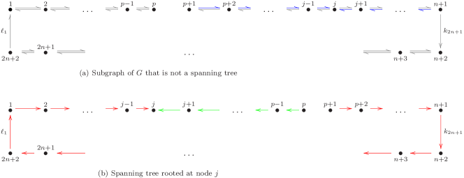
Figure 2. (a) Subgraph obtained from $G$ by removing edges $p\to p+1$ and $p\leftarrow p+1$. To obtain a subgraph $T$ for which the undirected graph $T^{*}$ is acyclic and connected, choose one edge from each gray pair of reversible edges. By choosing all the blue edges, one obtains two directed paths ending at $j$: one connecting the nodes $p+1$,…, $j-1$ to $j$ and the other connecting $j+1$, …, $n+1$ to $j$. No choice of edges, however, will connect any of the following nodes to $j$: $n+2$, …, $2n+2$ and $1$, …, $p$. Thus, any such subgraph will have at least two sinks. (b) Spanning tree $T_{j,p}$ (of $G$ from Fig. 1) rooted at $j$; this tree consists of two paths, one from $p$ to $j$ (green, counter-clockwise) and one from $p+1$ to $j$ (red, clockwise).

Now we can determine the directed spanning trees of $G$ (recall Definition A.1):

Proposition A.4 (Directed spanning trees of $G$ from Fig. 1).

For the directed graph $G$ in Fig. 1, let $j$ and $p$ be integers such that

$$1\leq j\leq p\leq n+1\quad{\rm or}\quad n+2\leq j\leq p\leq 2n+2~{}.$$ (A.1)

Let $T_{j,p}$ be the subgraph of $G$ that contains all nodes of $G$ and for which the edges are comprised of:

1. if $j\neq n+1,2n+2$:

   1. the clockwise path from node $p+1$ to $j$, and

   2. the counter-clockwise path from $p$ to $j$ (cf. Fig. 2(b)).

2. if $j=n+1$ or $j=2n+2$, the clockwise path from node $j+1$ to $j$ (where $j+1:=1$ if $j=2n+2$).

Then $T_{j,p}$ is a directed spanning tree rooted at node $j$ that does not contain the edges $p\to p+1$ or $p\leftarrow p+1$ (where $p+1:=1$ if $p=2n+2$). Conversely, every spanning tree of $G$ has this form.

Proof.

Assume that $T_{j,p}$ is a subgraph as described in the proposition. By Definition A.1 and Remark A.3, it remains only to show that there exists a path from every node $v\neq j$ to $j$. Indeed, by points (1) and (2), every node belongs to a path that ends in $j$.

Conversely, let $T$ be a spanning tree of $G$ rooted at $j$. By Remark A.3, there exists a node $p$ such that $T$ contains neither $p\to p+1$ nor $p\leftarrow p+1$, so it suffices to check that condition (A.1) holds and the edges of $T$ satisfy points (1) and (2). We first assume that $p$ violates condition (A.1). By symmetry between the two cases, we need only consider the case when $1\leq j\leq n+1$ and $p\in\{1,\dots,j-1\}\cup\{n+2,\dots,2n+2\}$. If $p\in\{1,\dots,j-1\}$, then there is no path in $T$ from $p$ to $j$; similarly, if $p\in\{n+2,\dots,2n+2\}$, then there is no path from $n+2$ to $j$ (cf. Fig. 2). Thus, $T$ is not a spanning tree rooted at $j$, which is a contradiction. Thus, $T$ must satisfy condition (A.1), so it remains only to show that it must satisfy points (1) and (2) as well. Indeed in the first case (that is, if $j\neq n+1,2n+2$), the paths (A) and (B) are the unique paths in $G$ that do not use $p\to p+1$ to reach $j$ from $p+1$ and $p$, respectively, and all nodes except $j$ lie on exactly one of these paths, so the two paths comprise the edges of $T$. Similarly, in the remaining case (if $j=n+1$ or $j=2n+2$), the clockwise path from node $j+1$ to $j$ is the unique path in $G$ from $j+1$ to $j$, and all nodes lie along the path (note that $j=p$ in this case). This completes the proof. ∎

We note the following corollary of Proposition A.4:

Corollary A.5.

For the directed graph $G$ in Fig. 1, the number of spanning trees rooted at $j$ is

• $n+2-j$, if $j\in\{1$, …, $n+1\}$

• $2n+3-j$, if $j\in\{n+2$, …, $2n+2\}$.

Consequently the number of spanning trees rooted at $j$ is at most $n+1$.

Now we turn to the kernel of $A_{\kappa}^{t}$. In Corollary 5.1, we argued that $\ker(A_{\kappa}^{t})$ is spanned by a positive vector. This is a consequence of [38, Lemma 2], which built on the well-known Matrix-Tree Theorem of algebraic combinatorics [37, §5.6], and also gives an explicit formula for this vector. For this, we need some more notation:
Notation. Following [38], for a directed spanning tree $T$ of an edge-labeled directed graph $G$, we denote by $L(T)$ the product of all edge labels in the spanning tree $T$:

$$L(T):=\prod_{y_{i}\overset{a}{\to}y_{j}\in T}a\ .$$ (A.2)

Note that $L(T)>0$, as it is a product of rate constants.

Proposition A.6.

Recall the spanning trees $T_{j,p}$ of $G$ from Fig. 1. For the matrix $\tilde{A}_{\kappa}^{t}$ displayed in (4.10) for the translated network (4.1), the nullspace is spanned by the positive vector $\rho\in\mathbb{R}_{+}^{2n+2}$ whose coordinates are given below:

$$\rho_{j}=\begin{cases}\displaystyle\sum_{p=j}^{n+1}L(T_{j,p})&{\rm if~{}}1\leq j\leq n+1\\ \displaystyle\sum_{i=j-(n+1)}^{n+1}L(T_{j,n+1+i})&{\rm if~{}}n+2\leq j\leq 2n+2~{}.\end{cases}$$ (A.3)

The terms $L(T_{j,p})$ are defined in eq. (A.4) below.

Proof.

Proposition A.4 and application of [38, Lemma 2] to $G$ from Fig. 1. ∎

Next we will compute the product $L(T_{j,p})$ associated to each spanning tree $T_{j,p}$ of $G$. To this end, we recall the labeling of reactions between adjacent nodes $j$ and $j+1$ for $1\leq j\leq n-1$:

For a node $j$ with $n+2\leq j\leq 2n+1$, we write $j$ as $j=n+1+i$ (so, $1\leq i\leq n+1$) and recall the labeling of reactions between adjacent nodes $j$ and $j+1$:

Now we use Proposition A.4 to compute $L(T_{j,p})$, for a spanning tree $T_{j,p}$ of $G$:

• if $1\leq j\leq n$, the tree $T_{j,p}$ splits into four paths:

  1. $p+1\to\cdots\to n+2$, with product of edge labels $k_{2n+1}\,\prod_{i=p+1}^{n}k_{2i-1}=\prod_{i=p+1}^{n+1}k_{2i-1}$,

  2. $n+2\to\cdots\to 1$, with product of edge labels $\ell_{1}\prod_{i=1}^{n},\ell_{2(n+1-i)+1}=\prod_{i=1}^{n+1}\ell_{2(n+1-i)+1}$,

  3. $1\to\cdots\to j$, with product of edge labels $\prod_{i=1}^{j-1}k_{2i-1}$,

  4. $p\to\cdots\to j$, with product of edge labels $\prod_{i=j}^{p-1}k_{2i}$.

• if $j=n+1$ (so, $p=n+1$, by Proposition A.4), the tree $T_{j,p}$ splits into two paths:

  1. $n+2\to\cdots\to 1$, with product of edge labels $\prod_{i=1}^{n+1}\ell_{2(n+1-i)+1}$, as in (b) in the previous case.

  2. $1\to\cdots\to n+1$, with product of edge labels $\prod_{i=1}^{n}k_{2i-1}$.

• if $n+2\leq j\leq 2n+1$, write $j=n+1+j_{0}$ and $p=n+1+p_{0}$, and then split $T_{j,p}$ into four paths (cf. Fig. 2(b)):

  1. $p+1\to\cdots\to 1$, with product of edge labels $\ell_{1}\prod_{i=p_{0}+1}^{n}\ell_{2(n+1-i)+1}=\prod_{i=p_{0}+1}^{n+1}\ell_{2(n+1-i)+1}$,

  2. $1\to\cdots\to n+2$, with product of edge labels $k_{2n+1}\prod_{i=1}^{n}k_{2i-1}=\prod_{i=1}^{n+1}k_{2i-1}$,

  3. $n+2\to\cdots\to j$, with product of edge labels $\prod_{i=1}^{j_{0}-1}\ell_{2(n+1-i)+1}$,

  4. $p\to\cdots\to j$, with product of edge labels $\prod_{i=j_{0}}^{p_{0}-1}\ell_{2(n+1-i)}$.

• if $j=2n+2$ (so, $p=2n+2$, by Proposition A.4), the tree $T_{j,p}$ splits into two paths:

  1. $1\to\cdots\to n+2$, with product of edge labels $\prod_{i=1}^{n+1}k_{2i-1}$, as in (b) in the previous case,

  2. $n+2\to\cdots\to 2n+2$, with product of edge labels $\prod_{i=1}^{n}\ell_{2(n+1-i)+1}$.

Thus, by definition (A.2), we obtain for $L(T_{j,p})$, where for $i_{1}<i_{0}$ we adopt the standard convention $\prod_{i=i_{0}}^{i_{1}}\alpha_{i}:=1$ for the empty product, and, as before, $j_{0}:=j-(n+1)$ and $p_{0}:=p-(n+1)$:

$$L(T_{j,p})=\begin{cases}\displaystyle\prod_{i=1}^{n+1}\ell_{2(n+1-i)+1}\cdot\prod_{i=1}^{j-1}k_{2i-1}\cdot\prod_{i=j}^{p-1}k_{2i}\cdot\prod_{i=p+1}^{n+1}k_{2i-1}&{\rm if~{}}1\leq j\leq n\\ \displaystyle\prod_{i=1}^{n+1}\ell_{2(n+1-i)+1}\cdot\prod_{i=1}^{n}k_{2i-1}&{\rm if~{}}j=n+1\\ \displaystyle\prod_{i=1}^{n+1}k_{2i-1}\cdot\prod_{i=1}^{j_{0}-1}\ell_{2(n+1-i)+1}\cdot\prod_{i=j_{0}}^{p_{0}-1}\ell_{2(n+1-i)}\cdot\prod_{i=p_{0}+1}^{n+1}\ell_{2(n+1-i)+1}&{\rm if~{}}n+2\leq j\leq 2n+1\\ \displaystyle\prod_{i=1}^{n+1}k_{2i-1}\cdot\prod_{i=1}^{n}\ell_{2(n+1-i)+1}&{\rm if~{}}j=2n+2~{}.\end{cases}$$ (A.4)

References

- [1] David F. Anderson, Global asymptotic stability for a class of nonlinear chemical equations, SIAM J. Appl. Math. 68 (2008), no. 5, 1464–1476.
- [2] David Angeli, Patrick De Leenheer, and Eduardo Sontag, Graph-theoretic characterizations of monotonicity of chemical networks in reaction coordinates, J. Math. Biol. 61 (2010), no. 4, 581–616.
- [3] David Angeli, Patrick De Leenheer, and Eduardo D. Sontag, A petri net approach to the study of persistence in chemical reaction networks, Mathematical Biosciences 210 (2007), no. 2, 598 – 618.
- [4] David Angeli and Eduardo D. Sontag, Translation-invariant monotone systems, and a global convergence result for enzymatic futile cycles, Nonlinear Anal. Real World Appl. 9 (2008), no. 1, 128–140.
- [5] Kazuhiro Aoki, Koichi Takahashi, Kazunari Kaizu, and Michiyuki Matsuda, A quantitative model of erk map kinase phosphorylation in crowded media, Sci. Rep. 3 (2013).
- [6] Murad Banaji and Gheorghe Craciun, Graph-theoretic approaches to injectivity and multiple equilibria in systems of interacting elements, Commun. Math. Sci. 7 (2009), no. 4, 867–900.
- [7] Murad Banaji and Janusz Mierczyński, Global convergence in systems of differential equations arising from chemical reaction networks, J. Differential Equations 254 (2013), no. 3, 1359–1374.
- [8] Murad Banaji and Casian Pantea, Some results on injectivity and multistationarity in chemical reaction networks, preprint, http://arXiv.org/abs/1309.6771 (2013).
- [9] C. Conradi, J. Saez-Rodriguez, E.-D. Gilles, and J. Raisch, Using Chemical Reaction Network Theory to discard a kinetic mechanism hypothesis, IEEE Proc. Systems Biology (now IET Systems Biology) 152 (2005), no. 4, 243–248.
- [10] Carsten Conradi, Dietrich Flockerzi, and Jörg Raisch, Multistationarity in the activation of a MAPK: parametrizing the relevant region in parameter space, Math. Biosci. 211 (2008), no. 1, 105–131.
- [11] Carsten Conradi and Maya Mincheva, Catalytic constants enable the emergence of bistability in dual phosphorylation, Journal of the Royal Society, Interface 11 (2014), no. 95.
- [12] Pete Donnell and Murad Banaji, Local and global stability of equilibria for a class of chemical reaction networks, SIAM J. Appl. Dyn. Syst. 12 (2013), no. 2, 899–920.
- [13] Pete Donnell, Murad Banaji, Anca Marginean, and Casian Pantea, CoNtRol: an open source framework for the analysis of chemical reaction networks, Bioinformatics (2014), to appear.
- [14] R. John Ellis, Macromolecular crowding: an important but neglected aspect of the intracellular environment, Current Opinion in Structural Biology 11 (2001), no. 1, 114 – 119.
- [15] Phillipp Ellison, Martin Feinberg, Haixia Ji, and Daniel Knight, Chemical Reaction Network Toolbox, 2011, Available at http://www.crnt.osu.edu/CRNTWin.
- [16] Martin Feinberg, Multiple steady states for chemical reaction networks of deficiency one, Arch. Rational Mech. Anal. 132 (1995), no. 4, 371–406.
- [17] Elisenda Feliu and Carsten Wiuf, Enzyme-sharing as a cause of multi-stationarity in signalling systems, J. R. Soc. Interface 9 (2012), no. 71, 1224–1232.
- [18] by same author, Simplifying biochemical models with intermediate species, J. R. Soc. Interface 10 (2013), no. 87.
- [19] D. Flockerzi, K. Holstein, and C. Conradi, N-site phosphorylation systems with 2N-1 steady states, Bulletin of Mathematical Biology 76 (2014), no. 8, 1892–1916.
- [20] Manoj Gopalkrishnan, Ezra Miller, and Anne Shiu, A geometric approach to the global attractor conjecture, SIAM J. Appl. Dyn. Syst. 13 (2014), no. 2, 758–797.
- [21] Jeremy Gunawardena, Multisite protein phosphorylation makes a good threshold but can be a poor switch, PNAS 102 (2005), no. 41, 14617–14622.
- [22] by same author, Distributivity and processivity in multisite phosphorylation can be distinguished through steady-state invariants, Biophys. J. 93 (2007), no. 11, 3828–3834.
- [23] Juliette Hell and Alan D. Rendall, A proof of bistability for the dual futile cycle, preprint, http://arxiv.org/abs/1404.0394 (2014).
- [24] Katharina Holstein, Dietrich Flockerzi, and Carsten Conradi, Multistationarity in sequential distributed multisite phosphorylation networks, Bull. Math. Biol. 75 (2013), no. 11, 2028–2058.
- [25] Matthew D. Johnston, Translated chemical reaction networks, Bull. Math. Biol. 76 (2014), no. 6, 1081–1116.
- [26] Badal Joshi and Anne Shiu, Simplifying the Jacobian criterion for precluding multistationarity in chemical reaction networks, SIAM J. Appl. Math. 72 (2012), no. 3, 857–876.
- [27] Arjun Kumar Manrai and Jeremy Gunawardena, The geometry of multisite phosphorylation, Biophys. J. 95 (2008), no. 12, 5533–5543.
- [28] Guy Marin and Gregory S. Yablonsky, Kinetics of chemical reactions, Wiley-VCH, Wienheim, Germany, 2011.
- [29] Nick I. Markevich, Jan B. Hoek, and Boris N. Kholodenko, Signaling switches and bistability arising from multisite phosphorylation in protein kinase cascades, J. Cell Biol. 164 (2004), no. 3, 353–359.
- [30] S. Müller, E. Feliu, G. Regensburger, C. Conradi, A. Shiu, and A. Dickenstein, Sign conditions for injectivity of generalized polynomial maps with applications to chemical reaction networks and real algebraic geometry, preprint, http://arxiv.org/abs/1311.5493 (2013).
- [31] Parag Patwardhan and W. Todd Miller, Processive phosphorylation: Mechanism and biological importance, Cellular Signalling 19 (2007), no. 11, 2218–2226.
- [32] Mercedes Pérez Millán, Alicia Dickenstein, Anne Shiu, and Carsten Conradi, Chemical reaction systems with toric steady states, Bull. Math. Biol. 74 (2012), no. 5, 1027–1065.
- [33] Mercedes Pérez Millán and Adrián G. Turjanski, MAPK’s networks and their capacity for multistationarity due to toric steady states, preprint, http://arxiv.org/abs/1403.6702 (2014).
- [34] Carlos Salazar and Thomas Höfer, Multisite protein phosphorylation —- from molecular mechanisms to kinetic models, FEBS Journal 276 (2009), no. 12, 3177–3198.
- [35] G. Shinar and M. Feinberg, Concordant chemical reaction networks, Math. Biosci. 240 (2012), no. 2, 92–113.
- [36] Hal L. Smith, Monotone dynamical systems: An introduction to the theory of competitive and cooperative systems, Mathematical Surveys and Monographs, vol. 41, American Mathematical Society, Providence, RI, 1995.
- [37] Richard P. Stanley, Enumerative combinatorics. Vol. 2, Cambridge Studies in Advanced Mathematics, vol. 62, Cambridge University Press, Cambridge, 1999.
- [38] Matthew Thomson and Jeremy Gunawardena, The rational parameterisation theorem for multisite post-translational modification systems, J. Theoret. Biol. 261 (2009), no. 4, 626–636.
- [39] by same author, Unlimited multistability in multisite phosphorylation systems, Nature 460 (2009), 274–277.
- [40] Liming Wang and Eduardo D. Sontag, On the number of steady states in a multiple futile cycle, J. Math. Biol. 57 (2008), no. 1, 29–52.