Stable Numerical Approximation of Two-Phase Flow with a Boussinesq–Scriven Surface Fluid

Abstract

We consider two-phase Navier–Stokes flow with a Boussinesq–Scriven surface fluid. In such a fluid the rheological behaviour at the interface includes surface viscosity effects, in addition to the classical surface tension effects. We introduce and analyze parametric finite element approximations, and show, in particular, stability results for semi-discrete versions of the methods, by demonstrating that a free energy inequality also holds on the discrete level. We perform several numerical simulations for various scenarios in two and three dimensions, which illustrate the effects of the surface viscosity.

Key words. incompressible two-phase flow, surface viscosity, Boussinesq–Scriven surface fluid, finite elements, parametric method, stability

AMS subject classifications. 35Q35, 65M12, 76D05, 76M10

1 Introduction

Fluid interfaces typically have their own dynamic properties and, in particular, a surface stress tensor, involving interfacial shear and dilatational viscosities, can have a significant effect on the dynamics. Surface tension effects on a fluid interface are well-known, and in this case the stresses acting on the interface are balanced by the surface tension and the curvature of the interface. However, in systems with high surface area to volume ratios, such as micro bubbles, blood cells, dispersions of vesicles and emulsions, the dynamics of the system are also highly influenced by the dynamics on the interface. Hence one can argue, see e.g. ?, that a more detailed study of the stress-deformation behaviour of interfaces is highly relevant for many disciplines, e.g. interface science, biophysics, pharmaceutical science, polymer physics, food science and engineering.

If only surface tension effects are taken into account in the surface stress tensor $\underline{\underline{\sigma}}\rule{0.0pt}{0.0pt}_{\Gamma}$, one obtains the form

$$\underline{\underline{\sigma}}\rule{0.0pt}{0.0pt}_{\Gamma}=\gamma\,\underline{\underline{\mathcal{P}}}\rule{0.0pt}{0.0pt}_{\Gamma},$$ (1.1)

where $\underline{\underline{\mathcal{P}}}\rule{0.0pt}{0.0pt}_{\Gamma}$ is the projection to the tangent space of the interfacial surface $\Gamma$, and $\gamma$ is the surface tension, which in the simplest case is constant. In this case the stress balance on the interface is given as

$$-\nabla_{\!s}\,.\,\underline{\underline{\sigma}}\rule{0.0pt}{0.0pt}_{\Gamma}=[\underline{\underline{\sigma}}\rule{0.0pt}{0.0pt}\,\vec{\nu}]^{+}_{-}\qquad\Leftrightarrow\qquad-\gamma\,\varkappa\,\vec{\nu}=[\underline{\underline{\sigma}}\rule{0.0pt}{0.0pt}\,\vec{\nu}]^{+}_{-}\,.$$ (1.2)

Here $\nabla_{\!s}\,.$ is the surface divergence, $[\,\cdot\,]^{+}_{-}$ denotes the jump of a quantity across the interface, $\underline{\underline{\sigma}}\rule{0.0pt}{0.0pt}$ denotes the bulk fluid stress tensor, $\vec{\nu}$ is the unit normal to the interface, and $\varkappa$ is the mean curvature, we refer to Section 2 for the precise definitions. Equation (1.1) expresses the momentum balance at a dividing surface, see e.g. ?. When the surface tension coefficient in (1.1) is not constant, which is the case when a surface active agent has an effect on the surface tension, the stress balance (1.2) becomes

$$-\gamma\,\varkappa\,\vec{\nu}-\nabla_{\!s}\,\gamma=[\underline{\underline{\sigma}}\rule{0.0pt}{0.0pt}\,\vec{\nu}]^{+}_{-}\,,$$

which in turn gives rise to discontinuities in the tangential components of the bulk fluid stresses at the surface. However, in general other interfacial properties, such as the resistance of an interface to deformation, have to be taken into account. This is particularly relevant in cases, where the interface is not clean. For systems with species that adsorb at the interface, like emulsions or foams stabilized by surfactants and proteins, it is expected that the surface stresses have a pronounced effect on the dynamics. Therefore the interest in surface rheology has increased significantly in the last twenty years, see e.g. ?. One key difference between bulk and surface rheology is that in the bulk phase one usually assumes incompressibility, whereas this assumption often does not hold for interfaces – biomembranes are a notable exception, see e.g. ?. The general momentum balance, which generalizes (1.2), now, in addition, has to take the surface momentum and a generalized stress tensor, involving surface shear and dilatational viscosities, into account. The overall momentum balance on the surface then reads as

$$\partial_{t}^{\bullet}\,(\rho_{\Gamma}\,\vec{u})+(\nabla_{\!s}\,.\,\vec{u})\,\rho_{\Gamma}\,\vec{u}-\nabla_{\!s}\,.\,\underline{\underline{\sigma}}\rule{0.0pt}{0.0pt}_{\Gamma}=[\underline{\underline{\sigma}}\rule{0.0pt}{0.0pt}\,\vec{\nu}]_{-}^{+}\,,$$ (1.3)

with the surface stress tensor now given by

$$\underline{\underline{\sigma}}\rule{0.0pt}{0.0pt}_{\Gamma}=2\,\mu_{\Gamma}\,\underline{\underline{D}}\rule{0.0pt}{0.0pt}_{s}(\vec{u})+(\lambda_{\Gamma}\,\nabla_{\!s}\,.\,\vec{u}+\gamma)\,\underline{\underline{\mathcal{P}}}\rule{0.0pt}{0.0pt}_{\Gamma}\,.$$

Here $\rho_{\Gamma}$ is the surface material density, $\vec{u}$ is the fluid velocity, $\partial_{t}^{\bullet}$ is the material derivative on the interface, $\mu_{\Gamma}$ is the surface shear viscosity, $\mu_{\Gamma}+\lambda_{\Gamma}$ is the surface dilatational viscosity and $\underline{\underline{D}}\rule{0.0pt}{0.0pt}_{s}(\vec{u})=\tfrac{1}{2}\,\underline{\underline{\mathcal{P}}}\rule{0.0pt}{0.0pt}_{\Gamma}\,(\nabla_{\!s}\,\vec{u}+(\nabla_{\!s}\,\vec{u})^{T})\,\underline{\underline{\mathcal{P}}}\rule{0.0pt}{0.0pt}_{\Gamma}$ is the interfacial rate-of-deformation tensor. This tensor describes how the lengths of curves on the surface change, and how the angles between intersecting curves change with the flow.

Although, at first glance, the surface momentum equation looks very similar to the bulk momentum equation, it turns out that new geometric quantities appear. For example, we note that in $\nabla_{\!s}\,.\,\vec{u}$ we take the divergence of a non-tangential vector field, which for alternative formulations of (1.3) would lead to a curvature term. In particular, splitting $\vec{u}$ into its normal part $(\vec{u}\,.\,\vec{\nu})\,\vec{\nu}$ and its tangential part $\vec{u}_{\rm tan}=\vec{u}-(\vec{u}\,.\,\vec{\nu})\,\vec{\nu}$ gives $\nabla_{\!s}\,.\,\vec{u}=\nabla_{\!s}\,.\,\vec{u}_{\rm tan}-\vec{u}\,.\,\vec{\nu}\,\varkappa$; see e.g. ?.

For the surface material density $\rho_{\Gamma}$ the mass balance law

$$\partial_{t}^{\bullet}\,\rho_{\Gamma}+(\nabla_{\!s}\,.\,\vec{u})\,\rho_{\Gamma}=0$$ (1.4)

holds on the surface. Hence (1.3) and (1.4) is a compressible Navier–Stokes system on an evolving surface with a forcing $[\underline{\underline{\sigma}}\rule{0.0pt}{0.0pt}\,\vec{\nu}]^{+}_{-}$ arising from bulk stresses. In this paper we also allow for an insoluble surface active agent (surfactant), whose concentration we denote by $\psi$. We then require that the advection-diffusion equation

$$\partial_{t}^{\bullet}\,\psi+(\nabla_{\!s}\,.\,\vec{u})\,\psi-\nabla_{\!s}\,.\,(\mathcal{D}_{\Gamma}\,\nabla_{\!s}\,\psi)=0\,,$$ (1.5)

with a diffusion coefficient $\mathcal{D}_{\Gamma}$, has to hold on the interface. In this case, the surface viscosities $\lambda_{\Gamma}$, $\mu_{\Gamma}$ and the surface tension $\gamma$ may depend on $\psi$. The system (1.3)–(1.5) then has to be coupled to the classical incompressible Navier–Stokes system in the bulk, and we refer to Section 2 for the details.

The first ideas, which later lead to the surface fluid model discussed above, are due to ?, and the approach of Boussinesq was later generalized to arbitrary moving and deforming surfaces by ?. Hence, one speaks of a Boussinesq–Scriven surface fluid, and we refer to the book ? for more details on the physics of the model and for experiments on Boussinesq–Scriven surface fluids.

The mathematical literature on models involving Boussinesq–Scriven surface fluids is very sparse. We refer to ?, who initiated the rigorous mathematical study of two-phase flows with surface viscosity in the case $\rho_{\Gamma}=0$, i.e. when no separate mass balance is considered. To the best knowledge of the authors, only the paper by ? contains numerical simulations of a two-phase flow including a Boussinesq–Scriven surface fluid. Also in that paper the surface material density was set to be zero and no surfactants were considered. It is the goal of this paper to introduce a stable finite element method for two-phase flow with a Boussinesq–Scriven interface stress tensor, which allows for a surface material density and an insoluble surfactant. Besides showing stability results, we also present numerical simulations in two and three dimensions, which show different phenomena arising from the surface viscosity effects.

Let us state the main features of the topics studied in this paper.

• Our approach is based on a parametric finite element method for the numerical approximation of the interface. Such an approach, in the context of a purely geometric evolution of the interface, was introduced by ?, see also the review article ?. We also use the techniques of ? for the approximation of partial differential equations on surfaces.

• For one variant of our introduced approximations, based on the present authors’ work, see ????, the parameterization of the evolving interface has good mesh properties and, in contrast to other parametric approaches, no remeshing is needed in practice.

• A suitable variational formulation of the complex conditions at the free boundary is introduced, which allows one to show stability of semi-discrete (discrete in space, continuous in time) versions of the schemes. This extends the present authors’ work on the stable numerical approximation of two-phase flow with insoluble surfactant, see ?, by including surface viscosity effects and a surface material density.

• Fully discrete finite element approximations are introduced, which lead to linear systems of equation at each time step. In particular, existence and uniqueness of the discrete solutions can be shown. If no surface material density is present, then stability can be shown also for these fully discrete variants.

• Conservation properties and non-negativity properties of the surface material density and the surfactant can be shown for the discretized systems.

• We present several numerical simulations in two and three space dimensions, which demonstrate the convergence of the scheme and illustrate several effects of surface viscosity. For example, in a shearing experiment one observes that bubbles with higher surface viscosities are much less elongated.

The study of numerical methods for two-phase flows is a very active area, and the available numerical approaches can be broadly grouped into three different categories: parametric front tracking methods, such as the approximations presented in this paper, level set methods and phase field methods; see the introduction in ?. For more details, and for further background information on the various approaches, we refer, for example, to ?????????. We remark that only ? have considered the case of a Boussinesq–Scriven surface fluid numerically.

The outline of the paper is as follows. In Section 2 we give a mathematical formulation of the Navier–Stokes two-phase problem for a Boussinesq–Scriven surface fluid. Section 3 states two semi-discrete approximations of the problem together with several analytical results such as stability, and conservation and non-negativity properties of the approximations to the surface material density and the surfactant concentration. In Section 4 the corresponding fully discrete approximations are introduced. Section 5 discusses some issues concerning the practical implementation of the method, in particular, the assembly of the bulk-interface cross terms. Finally, in Section 6 several numerical computations are presented.

2 Mathematical setting

Let $\Omega\subset\mathbb{R}^{d}$ be a given domain, where $d=2$ or $d=3$. We now seek a time dependent interface $(\Gamma(t))_{t\in[0,T]}$, $\Gamma(t)\subset\Omega$, which for all $t\in[0,T]$ separates $\Omega$ into a domain $\Omega_{+}(t)$, occupied by one phase, and a domain $\Omega_{-}(t):=\Omega\setminus\overline{\Omega}_{+}(t)$, which is occupied by the other phase. Here the phases could represent two different liquids, or a liquid and a gas. Common examples are oil/water or water/air interfaces. See Figure 1 for an illustration.

Figure 1: The domain $\Omega$ in the case $d=2$.

For later use, we assume that $(\Gamma(t))_{t\in[0,T]}$ is a sufficiently smooth evolving hypersurface without boundary that is parameterized by $\vec{x}(\cdot,t):\Upsilon\to{\mathbb{R}}^{d}$, where $\Upsilon\subset{\mathbb{R}}^{d}$ is a given reference manifold, i.e. $\Gamma(t)=\vec{x}(\Upsilon,t)$. Then

$$\vec{\mathcal{V}}(\vec{z},t):=\vec{x}_{t}(\vec{q},t)\qquad\forall\ \vec{z}=\vec{x}(\vec{q},t)\in\Gamma(t)$$ (2.1)

defines the velocity of $\Gamma(t)$, and $\vec{\mathcal{V}}\,.\,\vec{\nu}$ is the normal velocity of the evolving hypersurface $\Gamma(t)$, where $\vec{\nu}(t)$ is the unit normal on $\Gamma(t)$ pointing into $\Omega_{+}(t)$. Moreover, we define the space-time surface

$${\mathcal{G}_{T}}:=\bigcup_{t\in[0,T]}\Gamma(t)\times\{t\}\,.$$ (2.2)

Let $\rho(t)=\rho_{+}\,\mathrm{\mathcal{X}}_{\Omega_{+}(t)}+\rho_{-}\,\mathrm{\mathcal{X}}_{\Omega_{-}(t)}$, with $\rho_{\pm}\in{\mathbb{R}}_{>0}$, denote the fluid densities, where here and throughout $\mathrm{\mathcal{X}}_{\mathcal{A}}$ defines the characteristic function for a set $\mathcal{A}$. Denoting by $\vec{u}:\Omega\times[0,T]\to{\mathbb{R}}^{d}$ the fluid velocity, by $\underline{\underline{\sigma}}\rule{0.0pt}{0.0pt}:\Omega\times[0,T]\to{\mathbb{R}}^{d\times d}$ the stress tensor, and by $\vec{f}:\Omega\times[0,T]\to{\mathbb{R}}^{d}$ a possible forcing, the incompressible Navier–Stokes equations in the two phases are given by

$$\rho\,(\vec{u}_{t}+(\vec{u}\,.\,\nabla)\,\vec{u})-\nabla\,.\,\underline{\underline{\sigma}}\rule{0.0pt}{0.0pt} =\vec{f}:=\rho\,\vec{f}_{1}+\vec{f}_{2}\qquad \mbox{in }\Omega_{\pm}(t)\,,$$ (2.3a)

$$\nabla\,.\,\vec{u} =0\qquad \mbox{in }\Omega_{\pm}(t)\,,$$ (2.3b)

$$[\vec{u}]_{-}^{+} =\vec{0}\qquad \mbox{on }\Gamma(t)\,,$$ (2.3c)

$$\vec{u} =\vec{0}\qquad \mbox{on }\partial_{1}\Omega\,,$$ (2.3d)

$$\vec{u}\,.\,\vec{\rm n}=0\,,\quad\underline{\underline{\sigma}}\rule{0.0pt}{0.0pt}\,\vec{\rm n}\,.\,\vec{\rm t} =0\quad\forall\ \vec{\rm t}\in\{\vec{\rm n}\}^{\perp}\qquad \mbox{on }\partial_{2}\Omega\,,$$ (2.3e)

where $\partial\Omega=\partial_{1}\Omega\cup\partial_{2}\Omega$, with $\partial_{1}\Omega\cap\partial_{2}\Omega=\emptyset$, denotes the boundary of $\Omega$ with outer unit normal $\vec{\rm n}$ and $\{\vec{\rm n}\}^{\perp}:=\{\vec{\rm t}\in{\mathbb{R}}^{d}:\vec{\rm t}\,.\,\vec{\rm n}=0\}$. Hence (2.3d) prescribes a no-slip condition on $\partial_{1}\Omega$, while (2.3e) prescribes a free-slip condition on $\partial_{2}\Omega$. As usual, $[\vec{u}]_{-}^{+}:=\vec{u}_{+}-\vec{u}_{-}$ denotes the jump in velocity across the interface $\Gamma(t)$, where here and throughout we employ the shorthand notation $\vec{g}_{\pm}:=\vec{g}\!\mid_{\Omega_{\pm}(t)}$ for a function $\vec{g}:\Omega\times[0,T]\to{\mathbb{R}}^{d}$; and similarly for scalar and matrix-valued functions. In addition, the stress tensor in (2.3a) is defined by

$$\underline{\underline{\sigma}}\rule{0.0pt}{0.0pt}=\mu\,(\nabla\,\vec{u}+(\nabla\,\vec{u})^{T})-p\,\underline{\underline{\rm Id}}\rule{0.0pt}{0.0pt}=2\,\mu\,\underline{\underline{D}}\rule{0.0pt}{0.0pt}(\vec{u})-p\,\underline{\underline{\rm Id}}\rule{0.0pt}{0.0pt}\,,$$ (2.4)

where $\underline{\underline{\rm Id}}\rule{0.0pt}{0.0pt}\in{\mathbb{R}}^{d\times d}$ denotes the identity matrix, $\underline{\underline{D}}\rule{0.0pt}{0.0pt}(\vec{u}):=\frac{1}{2}\,(\nabla\,\vec{u}+(\nabla\,\vec{u})^{T})$ is the rate-of-deformation tensor, with $\nabla\,\vec{u}=\left(\partial_{x_{j}}\,u_{i}\right)_{i,j=1}^{d}$. As usual, $\nabla\,.\,\underline{\underline{A}}\rule{0.0pt}{0.0pt}\in{\mathbb{R}}^{d}$ with $[\nabla\,.\,\underline{\underline{A}}\rule{0.0pt}{0.0pt}]_{l}=\nabla\,.\,\vec{A}_{l}$, $l=1\to d$, for $\underline{\underline{A}}\rule{0.0pt}{0.0pt}^{T}=[\vec{A}_{1}\ldots\vec{A}_{d}]\in\mathbb{R}^{d\times d}$. Moreover, $p:\Omega\times[0,T]\to{\mathbb{R}}$ is the pressure and $\mu(t)=\mu_{+}\,\mathrm{\mathcal{X}}_{\Omega_{+}(t)}+\mu_{-}\,\mathrm{\mathcal{X}}_{\Omega_{-}(t)}$, with $\mu_{\pm}\in{\mathbb{R}}_{>0}$, denotes the dynamic viscosities in the two phases.

Let $\rho_{\Gamma}(\cdot,t):\Gamma(t)\to{\mathbb{R}}_{\geq 0}$ denote the surface material density. Then on the free surface the following conditions need to hold:

$$\partial_{t}^{\bullet}\,\rho_{\Gamma}+(\nabla_{\!s}\,.\,\vec{u})\,\rho_{\Gamma} =0\qquad \mbox{on }\Gamma(t)\,,$$ (2.5a)

$$\partial_{t}^{\bullet}\,(\rho_{\Gamma}\,\vec{u})+(\nabla_{\!s}\,.\,\vec{u})\,\rho_{\Gamma}\,\vec{u}-\nabla_{\!s}\,.\,\underline{\underline{\sigma}}\rule{0.0pt}{0.0pt}_{\Gamma} =[\underline{\underline{\sigma}}\rule{0.0pt}{0.0pt}\,\vec{\nu}]_{-}^{+}\qquad \mbox{on }\Gamma(t)\,,$$ (2.5b)

$$\vec{\mathcal{V}}\,.\,\vec{\nu} =\vec{u}\,.\,\vec{\nu}\qquad \mbox{on }\Gamma(t)\,,$$ (2.5c)

see e.g. ? and ?, p. 18–19. Here $[\underline{\underline{\sigma}}\rule{0.0pt}{0.0pt}\,\vec{\nu}]_{-}^{+}:=\underline{\underline{\sigma}}\rule{0.0pt}{0.0pt}_{+}\,\vec{\nu}-\underline{\underline{\sigma}}\rule{0.0pt}{0.0pt}_{-}\,\vec{\nu}$ denotes the jump in normal stress across $\Gamma(t)$, $\nabla_{\!s}\,.\,$ denotes the surface divergence on $\Gamma(t)$, $\underline{\underline{\sigma}}\rule{0.0pt}{0.0pt}_{\Gamma}$ is the surface stress tensor and

$$\partial_{t}^{\bullet}\,\zeta=\zeta_{t}+(\vec{u}\,.\,\nabla)\,\zeta=\zeta_{t}+\vec{u}\,.\,\nabla\,\zeta\qquad\mbox{on }\Gamma(t)$$ (2.6)

denotes the material time derivative of $\zeta:{\mathcal{G}_{T}}\to{\mathbb{R}}$, and similarly for $\vec{\zeta}:{\mathcal{G}_{T}}\to{\mathbb{R}}^{d}$, i.e. $\partial_{t}^{\bullet}\,\vec{\zeta}=\vec{\zeta}_{t}+(\vec{u}\,.\,\nabla)\,\vec{\zeta}=\vec{\zeta}_{t}+(\nabla\,\vec{\zeta})\,\vec{u}$. We set $H^{1}({\mathcal{G}_{T}}):=\{\zeta\in L^{2}({\mathcal{G}_{T}}):\nabla_{\!s}\,\zeta\in L^{2}({\mathcal{G}_{T}}),\partial_{t}^{\bullet}\,\zeta\in L^{2}({\mathcal{G}_{T}})\}$. We stress that the derivative in (2.6) is well-defined, and depends only on the values of $\zeta$ on ${\mathcal{G}_{T}}$, even though $\zeta_{t}$ and $\nabla\,\zeta$ do not make sense separately; see e.g. ?, p. 324. The surface stress tensor is defined by

$$\underline{\underline{\sigma}}\rule{0.0pt}{0.0pt}_{\Gamma}=2\,\mu_{\Gamma}(\psi)\,\underline{\underline{D}}\rule{0.0pt}{0.0pt}_{s}(\vec{u})+(\lambda_{\Gamma}(\psi)\,\nabla_{\!s}\,.\,\vec{u}+\gamma(\psi))\,\underline{\underline{\mathcal{P}}}\rule{0.0pt}{0.0pt}_{\Gamma}\,,$$ (2.7)

where $\mu_{\Gamma}\in C({\mathbb{R}},{\mathbb{R}}_{\geq 0})$ is the interfacial shear viscosity, and $\lambda_{\Gamma}\in C({\mathbb{R}})$ is the second interfacial viscosity coefficient satisfying

$$\lambda_{\Gamma}(r)+\tfrac{2}{d-1}\,\mu_{\Gamma}(r)\geq 0\qquad\forall\ r\in{\mathbb{R}}\,.$$ (2.8)

In the special case that

$$\mu_{\Gamma}(r)=\overline{\mu}_{\Gamma}\in{\mathbb{R}}_{\geq 0}\quad\text{and}\quad\lambda_{\Gamma}(r)=\overline{\lambda}_{\Gamma}\in{\mathbb{R}}\qquad\forall\ r\in{\mathbb{R}}\,,$$ (2.9)

the constants $\overline{\lambda}_{\Gamma}$ and $\overline{\mu}_{\Gamma}$ are also called the first and second surface Lamé constants, respectively. In addition, $\gamma\in C^{1}([0,\psi_{\infty}))$, with $\psi_{\infty}>0$ and

$$\gamma^{\prime}(r)\leq 0\qquad\forall\ r\in[0,\psi_{\infty})\,,$$ (2.10)

denotes the surface tension. The interfacial viscosities and the surface tension depend on the surfactant concentration $\psi:{\mathcal{G}_{T}}\to[0,\psi_{\infty})$, recall (2.2). In addition,

$$\underline{\underline{\mathcal{P}}}\rule{0.0pt}{0.0pt}_{\Gamma}=\underline{\underline{\rm Id}}\rule{0.0pt}{0.0pt}-\vec{\nu}\otimes\vec{\nu}$$ (2.11a)

is the tangential projection at $$\Gamma(t)$$, and

$$\underline{\underline{D}}\rule{0.0pt}{0.0pt}_{s}(\vec{u})=\tfrac{1}{2}\,\underline{\underline{\mathcal{P}}}\rule{0.0pt}{0.0pt}_{\Gamma}\,(\nabla_{\!s}\,\vec{u}+(\nabla_{\!s}\,\vec{u})^{T})\,\underline{\underline{\mathcal{P}}}\rule{0.0pt}{0.0pt}_{\Gamma}$$ (2.11b)

is the interfacial rate-of-deformation tensor, where $\nabla_{\!s}=\underline{\underline{\mathcal{P}}}\rule{0.0pt}{0.0pt}_{\Gamma}\,\nabla=(\partial_{s_{1}},\ldots,\partial_{s_{d}})$ denotes the surface gradient on $\Gamma(t)$, and $\nabla_{\!s}\,\vec{u}=\left(\partial_{s_{j}}\,u_{i}\right)_{i,j=1}^{d}$.

The surfactant transport (with diffusion) on $\Gamma(t)$ is then given by

$$\partial_{t}^{\bullet}\,\psi+(\nabla_{\!s}\,.\,\vec{u})\,\psi-\nabla_{\!s}\,.\,(\mathcal{D}_{\Gamma}\,\nabla_{\!s}\,\psi)=0\qquad\mbox{on }\Gamma(t)\,,$$ (2.12)

where $\mathcal{D}_{\Gamma}\geq 0$ is a diffusion coefficient. The system (2.3a–e), (2.4), (2.5a–c), (2.7), (2.12) is closed with the initial conditions

$$\Gamma(0)=\Gamma_{0}\,,\quad\rho_{\Gamma}(\cdot,0)=\rho_{\Gamma,0}\quad\mbox{on }\Gamma_{0}\,,\quad\psi(\cdot,0)=\psi_{0}\quad\mbox{on }\Gamma_{0}\,,\quad\vec{u}(\cdot,0)=\vec{u}_{0}\qquad\mbox{in }\Omega\,,$$ (2.13)

where $\Gamma_{0}\subset\Omega$, $\rho_{\Gamma,0}:\Gamma_{0}\to{\mathbb{R}}_{\geq 0}$, $\psi_{0}:\Gamma_{0}\to[0,\psi_{\infty})$ and $\vec{u}_{0}:\Omega\to{\mathbb{R}}^{d}$ are given initial data.

With a view towards substituting (2.7) into (2.5b), we observe that

$$\nabla_{\!s}\,.\,\underline{\underline{\sigma}}\rule{0.0pt}{0.0pt}_{\Gamma} =2\,\mu_{\Gamma}(\psi)\,\nabla_{\!s}\,.\,\underline{\underline{D}}\rule{0.0pt}{0.0pt}_{s}(\vec{u})+\nabla_{\!s}\,.\left[(\lambda_{\Gamma}(\psi)\,\nabla_{\!s}\,.\,\vec{u}+\gamma(\psi))\,\underline{\underline{\mathcal{P}}}\rule{0.0pt}{0.0pt}_{\Gamma}\right]$$

$$=2\,\mu_{\Gamma}(\psi)\,\nabla_{\!s}\,.\,\underline{\underline{D}}\rule{0.0pt}{0.0pt}_{s}(\vec{u})+\nabla_{\!s}\,.\left[\lambda_{\Gamma}(\psi)\,(\nabla_{\!s}\,.\,\vec{u})\,\underline{\underline{\mathcal{P}}}\rule{0.0pt}{0.0pt}_{\Gamma}\right]+\gamma(\psi)\,\varkappa\,\vec{\nu}+\nabla_{\!s}\,\gamma(\psi)\,,$$ (2.14)

where $\nabla_{\!s}\,.\,\underline{\underline{A}}\rule{0.0pt}{0.0pt}\in{\mathbb{R}}^{d}$ with $[\nabla_{\!s}\,.\,\underline{\underline{A}}\rule{0.0pt}{0.0pt}]_{l}=\nabla_{\!s}\,.\,\vec{A}_{l}$, $l=1\to d$, for $\underline{\underline{A}}\rule{0.0pt}{0.0pt}^{T}=[\vec{A}_{1}\ldots\vec{A}_{d}]\in\mathbb{R}^{d\times d}$, and where we have noted that $\nabla_{\!s}\,.\,\vec{\nu}=\nabla\,.\,\vec{\nu}=-\varkappa$ implies that

$$\nabla_{\!s}\,.\,\underline{\underline{\mathcal{P}}}\rule{0.0pt}{0.0pt}_{\Gamma}=\varkappa\,\vec{\nu}\,.$$

Here $\varkappa$ denotes the mean curvature of $\Gamma(t)$, i.e. the sum of the principal curvatures of $\Gamma(t)$, where we have adopted the sign convention that $\varkappa$ is negative where $\Omega_{-}(t)$ is locally convex. In particular, it holds that

$$\Delta_{s}\,\vec{\rm}id=\varkappa\,\vec{\nu}=:\vec{\varkappa}\qquad\mbox{on $\Gamma(t)$}\,,$$ (2.15)

where $\Delta_{s}=\nabla_{\!s}\,.\,\nabla_{\!s}$ is the Laplace–Beltrami operator on $\Gamma(t)$.

In the case that the interface is non-material, i.e. when $\rho_{\Gamma}=0$, then the interface conditions (2.5a–c) simplify dramatically. In this case, on recalling (2.14), we are left with the following conditions to hold on $\Gamma(t)$:

$$[\underline{\underline{\sigma}}\rule{0.0pt}{0.0pt}\,\vec{\nu}]_{-}^{+} =-2\,\mu_{\Gamma}(\psi)\,\nabla_{\!s}\,.\,\underline{\underline{D}}\rule{0.0pt}{0.0pt}_{s}(\vec{u})-\nabla_{\!s}\,.\left[\lambda_{\Gamma}(\psi)\,(\nabla_{\!s}\,.\,\vec{u})\,\underline{\underline{\mathcal{P}}}\rule{0.0pt}{0.0pt}_{\Gamma}\right]-\gamma(\psi)\,\varkappa\,\vec{\nu}-\nabla_{\!s}\,\gamma(\psi)\,,$$ (2.16a)

$$\vec{\mathcal{V}}\,.\,\vec{\nu} =\vec{u}\,.\,\vec{\nu}\,.$$ (2.16b)

If, in addition, $\lambda_{\Gamma}(\psi)=\mu_{\Gamma}(\psi)=0$, then (2.16a,b) reduce to the interface conditions studied by the authors in ?, where a two-phase flow problem with insoluble surfactant is considered.

For later purposes, we introduce the surface energy function $F$, which satisfies

$$\gamma(r)=F(r)-r\,F^{\prime}(r)\qquad\forall\ r\in(0,\psi_{\infty})\,,$$ (2.17a)

and

$$\lim_{r\to 0}r\,F^{\prime}(r)=F(0)-\gamma(0)=0\,.$$ (2.17b)

This means in particular that

$$\gamma^{\prime}(r)=-r\,F^{\prime\prime}(r)\qquad\forall\ r\in(0,\psi_{\infty})\,.$$ (2.18)

It immediately follows from (2.18) and (2.10) that $F\in C([0,\psi_{\infty}))\cap C^{2}(0,\psi_{\infty})$ is convex. Typical examples for $\gamma$ and $F$ are given by

$$\gamma(r)=\overline{\gamma}\,(1-\beta\,r)\,,\quad F(r)=\overline{\gamma}\left[1+\beta\,r\left(\ln r-1\right)\right],\ \psi_{\infty}=\infty\,,$$ (2.19a)

which represents a linear equation of state, and by

$$\gamma(r)=\overline{\gamma}\left[1+\beta\,\psi_{\infty}\,\ln\left(1-\tfrac{r}{\psi_{\infty}}\right)\right],\quad F(r)=\overline{\gamma}\left[1+\beta\left(r\,\ln\tfrac{r}{\psi_{\infty}-r}+\psi_{\infty}\,\ln\tfrac{\psi_{\infty}-r}{\psi_{\infty}}\right)\right],$$ (2.19b)

the so-called Langmuir equation of state, where $\overline{\gamma}\in{\mathbb{R}}_{>0}$ and $\beta\in{\mathbb{R}}_{\geq 0}$ are further given parameters, where we note that the special case $\beta=0$ means that (2.19a,b) reduce to

$$F(r)=\gamma(r)=\overline{\gamma}\in{\mathbb{R}}_{>0}\qquad\forall\ r\in{\mathbb{R}}\,.$$ (2.20)

In the case (2.20) the surface tension no longer depends on the surfactant concentration $\psi$.

Before introducing our finite element approximation, we will state an appropriate weak formulation. With this in mind, we introduce the function spaces

$$\mathbb{U} :=\{\vec{\varphi}\in[H^{1}(\Omega)]^{d}:\vec{\varphi}=\vec{0}\ \mbox{ on }\partial_{1}\Omega\,,\ \vec{\varphi}\,.\,\vec{\rm n}=0\ \mbox{ on }\partial_{2}\Omega\}\,,\quad\mathbb{P}:=L^{2}(\Omega)\,,$$

$$\widehat{\mathbb{P}} :=\{\eta\in\mathbb{P}:\int_{\Omega}\eta\;{\rm d}{\cal L}^{d}=0\}\,,\quad\mathbb{V}:=L^{2}(0,T;\mathbb{U})\cap H^{1}(0,T;[L^{2}(\Omega)]^{d})\,,\quad\mathbb{S}:=H^{1}({\mathcal{G}_{T}})\,,$$

$$\mathbb{V}_{\Gamma} :=\{\vec{\varphi}\in\mathbb{V}:\vec{\varphi}\!\mid_{\mathcal{G}_{T}}\in[\mathbb{S}]^{d}\}\,.$$

Let $(\cdot,\cdot)$ and $\langle\cdot,\cdot\rangle_{\Gamma(t)}$ denote the $L^{2}$–inner products on $\Omega$ and $\Gamma(t)$, respectively. For later use we recall from ?, Def. 2.11 that

$$\left\langle\zeta,\nabla_{\!s}\,.\,\vec{\eta}\right\rangle_{\Gamma(t)}+\left\langle\nabla_{\!s}\,\zeta,\vec{\eta}\right\rangle_{\Gamma(t)}=-\left\langle\zeta\,\vec{\eta},\vec{\varkappa}\right\rangle_{\Gamma(t)}\qquad\forall\ \zeta\in H^{1}(\Gamma(t)),\,\vec{\eta}\in[H^{1}(\Gamma(t))]^{d}\,.$$ (2.21)

We remark that it follows from (2.21) that

$$\left\langle\gamma(\psi)\,\vec{\varkappa}+\nabla_{\!s}\,\gamma(\psi),\vec{\xi}\right\rangle_{\Gamma(t)}=\left\langle\gamma(\psi)\,\varkappa\,\vec{\nu}+\nabla_{\!s}\,\gamma(\psi),\vec{\xi}\right\rangle_{\Gamma(t)}=-\left\langle\gamma(\psi),\nabla_{\!s}\,.\,\vec{\xi}\right\rangle_{\Gamma(t)}\quad\forall\ \vec{\xi}\in\mathbb{U}\,.$$ (2.22)

We recall from ? that it follows from (2.3b–e) and (2.5c) that

$$(\rho\,(\vec{u}\,.\,\nabla)\,\vec{u},\vec{\xi}) =\tfrac{1}{2}\left[(\rho\,(\vec{u}\,.\,\nabla)\,\vec{u},\vec{\xi})-(\rho\,(\vec{u}\,.\,\nabla)\,\vec{\xi},\vec{u})-\langle[\rho]_{-}^{+}\,\vec{u}\,.\,\vec{\nu},\vec{u}\,.\,\vec{\xi}\rangle_{\Gamma(t)}\right]$$

$$\hskip 231.26378pt\qquad\forall\ \vec{\xi}\in[H^{1}(\Omega)]^{d}$$ (2.23)

and

$$\frac{\rm d}{{\rm d}t}(\rho\,\vec{u},\vec{\xi}) =(\rho\,\vec{u}_{t},\vec{\xi})+(\rho\,\vec{u},\vec{\xi}_{t})-\left\langle[\rho]_{-}^{+}\,\vec{u}\,.\,\vec{\nu},\vec{u}\,.\,\vec{\xi}\right\rangle_{\Gamma(t)}\qquad\forall\ \vec{\xi}\in\mathbb{V}\,,$$ (2.24)

respectively. Therefore, it holds that

$$(\rho\,\vec{u}_{t},\vec{\xi})=\tfrac{1}{2}\left[\frac{\rm d}{{\rm d}t}(\rho\,\vec{u},\vec{\xi})+(\rho\,\vec{u}_{t},\vec{\xi})-(\rho\,\vec{u},\vec{\xi}_{t})+\left\langle[\rho]_{-}^{+}\,\vec{u}\,.\,\vec{\nu},\vec{u}\,.\,\vec{\xi}\right\rangle_{\Gamma(t)}\right]\qquad\forall\ \vec{\xi}\in\mathbb{V}\,,$$

which on combining with (2.23) yields that

$$(\rho\,[\vec{u}_{t}+(\vec{u}\,.\,\nabla)\,\vec{u}],\vec{\xi})$$

$$\quad=\tfrac{1}{2}\left[\frac{\rm d}{{\rm d}t}(\rho\,\vec{u},\vec{\xi})+(\rho\,\vec{u}_{t},\vec{\xi})-(\rho\,\vec{u},\vec{\xi}_{t})+(\rho,[(\vec{u}\,.\,\nabla)\,\vec{u}]\,.\,\vec{\xi}-[(\vec{u}\,.\,\nabla)\,\vec{\xi}]\,.\,\vec{u})\right]\qquad\forall\ \vec{\xi}\in\mathbb{V}\,.$$ (2.25)

Moreover, it holds, on noting (2.3e) and (2.4), that for all $\vec{\xi}\in\mathbb{U}$

$$\int_{\Omega_{+}(t)\cup\Omega_{-}(t)}(\nabla\,.\,\underline{\underline{\sigma}}\rule{0.0pt}{0.0pt})\,.\,\vec{\xi}\;{\rm d}{\cal L}^{d}=-2\,(\mu\,\underline{\underline{D}}\rule{0.0pt}{0.0pt}(\vec{u}),\underline{\underline{D}}\rule{0.0pt}{0.0pt}(\vec{\xi}))+(p,\nabla\,.\,\vec{\xi})-\left\langle[\underline{\underline{\sigma}}\rule{0.0pt}{0.0pt}\,\vec{\nu}]_{-}^{+},\vec{\xi}\right\rangle_{\Gamma(t)}\,,$$ (2.26)

where we have also noted for symmetric matrices $\underline{\underline{A}}\rule{0.0pt}{0.0pt}\in{\mathbb{R}}^{d\times d}$ that $\underline{\underline{A}}\rule{0.0pt}{0.0pt}:\underline{\underline{B}}\rule{0.0pt}{0.0pt}=\underline{\underline{A}}\rule{0.0pt}{0.0pt}:\tfrac{1}{2}\,(\underline{\underline{B}}\rule{0.0pt}{0.0pt}+\underline{\underline{B}}\rule{0.0pt}{0.0pt}^{T})$ for all $\underline{\underline{B}}\rule{0.0pt}{0.0pt}\in{\mathbb{R}}^{d\times d}$.

Similarly to (2.6) we define the following time derivative that follows the parameterization $\vec{x}(\cdot,t)$ of $\Gamma(t)$, rather than $\vec{u}$. In particular, we let

$$\partial_{t}^{\circ}\,\zeta=\zeta_{t}+\vec{\mathcal{V}}\,.\,\nabla\,\zeta\qquad\forall\ \zeta\in H^{1}({\mathcal{G}_{T}})\,;$$ (2.27)

where we stress once again that this definition is well-defined, even though $\zeta_{t}$ and $\nabla\,\zeta$ do not make sense separately for a function $\zeta\in H^{1}({\mathcal{G}_{T}})$. On recalling (2.6) we obtain that

$$\partial_{t}^{\circ}=\partial_{t}^{\bullet}\qquad\text{if}\qquad\vec{\mathcal{V}}=\vec{u}\quad\text{on }\Gamma(t)\,.$$ (2.28)

We note that the definition (2.27) differs from the definition of $\partial^{\circ}$ in ?, p. 327, where $\partial^{\circ}\,\zeta=\zeta_{t}+(\vec{\mathcal{V}}\,.\,\vec{\nu})\,\vec{\nu}\,.\,\nabla\,\zeta$ for the “normal time derivative”. It holds that

$$\frac{\rm d}{{\rm d}t}\left\langle\chi,\zeta\right\rangle_{\Gamma(t)}=\left\langle\partial_{t}^{\circ}\,\chi,\zeta\right\rangle_{\Gamma(t)}+\left\langle\chi,\partial_{t}^{\circ}\,\zeta\right\rangle_{\Gamma(t)}+\left\langle\chi\,\zeta,\nabla_{\!s}\,.\,\vec{\mathcal{V}}\right\rangle_{\Gamma(t)}\qquad\forall\ \chi,\zeta\in H^{1}({\mathcal{G}_{T}})\,,$$ (2.29)

see ?, Lem. 5.2.

If $\vec{\cal V}=\vec{u}$ on $\Gamma(t)$, then it follows from (2.5b), (2.14), (2.28), (2.29) and (2.21) that

$$\frac{\rm d}{{\rm d}t}\left\langle\rho_{\Gamma}\,\vec{u},\vec{\xi}\right\rangle_{\Gamma(t)}+2\left\langle\mu_{\Gamma}(\psi)\,\underline{\underline{D}}\rule{0.0pt}{0.0pt}_{s}(\vec{u}),\underline{\underline{D}}\rule{0.0pt}{0.0pt}_{s}(\vec{\xi})\right\rangle_{\Gamma(t)}+\left\langle\lambda_{\Gamma}(\psi)\,\nabla_{\!s}\,.\,\vec{u},\nabla_{\!s}\,.\,\vec{\xi}\right\rangle_{\Gamma(t)}$$

$$\hskip 28.45274pt-\left\langle\gamma(\psi)\,\vec{\varkappa}+\nabla_{\!s}\,\gamma(\psi),\vec{\xi}\right\rangle_{\Gamma(t)}=\left\langle\rho_{\Gamma}\,\vec{u},\partial_{t}^{\circ}\,\vec{\xi}\right\rangle_{\Gamma(t)}+\left\langle[\underline{\underline{\sigma}}\rule{0.0pt}{0.0pt}\,\vec{\nu}]_{-}^{+},\vec{\xi}\right\rangle_{\Gamma(t)}\qquad\forall\ \vec{\xi}\in\mathbb{S}\,,$$ (2.30)

where we have noted for symmetric matrices $\underline{\underline{A}}\rule{0.0pt}{0.0pt}\in{\mathbb{R}}^{d\times d}$ that $\underline{\underline{\mathcal{P}}}\rule{0.0pt}{0.0pt}_{\Gamma}\,\underline{\underline{A}}\rule{0.0pt}{0.0pt}\,\underline{\underline{\mathcal{P}}}\rule{0.0pt}{0.0pt}_{\Gamma}:\underline{\underline{B}}\rule{0.0pt}{0.0pt}=\underline{\underline{\mathcal{P}}}\rule{0.0pt}{0.0pt}_{\Gamma}\,\underline{\underline{A}}\rule{0.0pt}{0.0pt}\,\underline{\underline{\mathcal{P}}}\rule{0.0pt}{0.0pt}_{\Gamma}:\tfrac{1}{2}\,\underline{\underline{\mathcal{P}}}\rule{0.0pt}{0.0pt}_{\Gamma}\,(\underline{\underline{B}}\rule{0.0pt}{0.0pt}+\underline{\underline{B}}\rule{0.0pt}{0.0pt}^{T})\,\underline{\underline{\mathcal{P}}}\rule{0.0pt}{0.0pt}_{\Gamma}$ for all $\underline{\underline{B}}\rule{0.0pt}{0.0pt}\in{\mathbb{R}}^{d\times d}$.

We are now in a position to state weak formulations of the Navier–Stokes two-phase flow problem for a Boussinesq–Scriven surface fluid that we consider in this paper. The natural weak formulation of the system (2.3a–e), (2.4), (2.5a–c), (2.7) and (2.12) is given as follows. Find $\Gamma(t)=\vec{x}(\Upsilon,t)$ for $t\in[0,T]$ with $\vec{\mathcal{V}}\in[L^{2}({\mathcal{G}_{T}})]^{d}$, and functions $\rho_{\Gamma}\in\mathbb{S}$, $\vec{u}\in\mathbb{V}_{\Gamma}$, $p\in L^{2}(0,T;\widehat{\mathbb{P}})$, $\vec{\varkappa}\in[L^{2}({\mathcal{G}_{T}})]^{d}$ and $\psi\in\mathbb{S}$ such that for almost all $t\in(0,T)$ it holds that

$$\frac{\rm d}{{\rm d}t}\left\langle\rho_{\Gamma},\zeta\right\rangle_{\Gamma(t)}=\left\langle\rho_{\Gamma},\partial_{t}^{\circ}\,\zeta\right\rangle_{\Gamma(t)}\quad\forall\ \zeta\in\mathbb{S}\,,$$ (2.31a)

$$\tfrac{1}{2}\left[\frac{\rm d}{{\rm d}t}(\rho\,\vec{u},\vec{\xi})+(\rho\,\vec{u}_{t},\vec{\xi})-(\rho\,\vec{u},\vec{\xi}_{t})+(\rho,[(\vec{u}\,.\,\nabla)\,\vec{u}]\,.\,\vec{\xi}-[(\vec{u}\,.\,\nabla)\,\vec{\xi}]\,.\,\vec{u})\right]+2\,(\mu\,\underline{\underline{D}}\rule{0.0pt}{0.0pt}(\vec{u}),\underline{\underline{D}}\rule{0.0pt}{0.0pt}(\vec{\xi}))$$

$$\quad-(p,\nabla\,.\,\vec{\xi})+\frac{\rm d}{{\rm d}t}\left\langle\rho_{\Gamma}\,\vec{u},\vec{\xi}\right\rangle_{\Gamma(t)}+2\left\langle\mu_{\Gamma}(\psi)\,\underline{\underline{D}}\rule{0.0pt}{0.0pt}_{s}(\vec{u}),\underline{\underline{D}}\rule{0.0pt}{0.0pt}_{s}(\vec{\xi})\right\rangle_{\Gamma(t)}$$

$$\quad+\left\langle\lambda_{\Gamma}(\psi)\,\nabla_{\!s}\,.\,\vec{u},\nabla_{\!s}\,.\,\vec{\xi}\right\rangle_{\Gamma(t)}-\left\langle\gamma(\psi)\,\vec{\varkappa}+\nabla_{\!s}\,\gamma(\psi),\vec{\xi}\right\rangle_{\Gamma(t)}$$

$$\quad=(\vec{f},\vec{\xi})+\left\langle\rho_{\Gamma}\,\vec{u},\partial_{t}^{\circ}\,\vec{\xi}\right\rangle_{\Gamma(t)}\qquad\forall\ \vec{\xi}\in\mathbb{V}_{\Gamma}\,,$$ (2.31b)

$$(\nabla\,.\,\vec{u},\varphi)=0\qquad\forall\ \varphi\in\widehat{\mathbb{P}}\,,$$ (2.31c)

$$\left\langle\vec{\mathcal{V}}-\vec{u},\vec{\chi}\right\rangle_{\Gamma(t)}=0\qquad\forall\ \vec{\chi}\in[L^{2}(\Gamma(t))]^{d}\,,$$ (2.31d)

$$\left\langle\vec{\varkappa},\vec{\eta}\right\rangle_{\Gamma(t)}+\left\langle\nabla_{\!s}\,\vec{\rm}id,\nabla_{\!s}\,\vec{\eta}\right\rangle_{\Gamma(t)}=0\qquad\forall\ \vec{\eta}\in[H^{1}(\Gamma(t))]^{d}\,,$$ (2.31e)

$$\frac{\rm d}{{\rm d}t}\left\langle\psi,\zeta\right\rangle_{\Gamma(t)}+\mathcal{D}_{\Gamma}\left\langle\nabla_{\!s}\,\psi,\nabla_{\!s}\,\zeta\right\rangle_{\Gamma(t)}=\left\langle\psi,\partial_{t}^{\circ}\,\zeta\right\rangle_{\Gamma(t)}\quad\forall\ \zeta\in\mathbb{S}\,,$$ (2.31f)

as well as the initial conditions (2.13), where in (2.31d) we have recalled (2.1). Here (2.31b) is derived from (2.3a) and (2.5b) by combining (2), (2.26) and (2.30), on noting (2.31d). The equations (2.31a,f) are derived, similarly to (2.30), from (2.5a) and (2.12), respectively, on noting (2.29) and (2.31d). Of course, it follows from (2.31d) and (2.28) that $\partial_{t}^{\circ}$ in (2.31a,b,f) can be replaced by $\partial_{t}^{\bullet}$.

In what follows we would like to derive an energy bound for a solution of (2.31a–f). All of the following considerations are formal, in the sense that we make the appropriate assumptions about the existence, boundedness and regularity of a solution to (2.31a–f). In particular, we assume that $\psi\in[0,\psi_{\infty})$. Choosing $\vec{\xi}=\vec{u}$ in (2.31b), $\varphi=p(\cdot,t)$ in (2.31c) and $\zeta=-\frac{1}{2}\,|\vec{u}\mid_{{\cal G}_{T}}\!\!|^{2}$ in (2.31a), and combining yields that

$$\tfrac{1}{2}\,\frac{\rm d}{{\rm d}t}\,\left[\|\rho^{\frac{1}{2}}\,\vec{u}\|_{0}^{2}+\left\langle\rho_{\Gamma}\,\vec{u},\vec{u}\right\rangle_{\Gamma(t)}\right]+2\,\|\mu^{\frac{1}{2}}\,\underline{\underline{D}}\rule{0.0pt}{0.0pt}(\vec{u})\|_{0}^{2}+2\left\langle\mu_{\Gamma}(\psi)\,\underline{\underline{D}}\rule{0.0pt}{0.0pt}_{s}(\vec{u}),\underline{\underline{D}}\rule{0.0pt}{0.0pt}_{s}(\vec{u})\right\rangle_{\Gamma(t)}$$

$$\hskip 28.45274pt+\left\langle\lambda_{\Gamma}(\psi)\,\nabla_{\!s}\,.\,\vec{u},\nabla_{\!s}\,.\,\vec{u}\right\rangle_{\Gamma(t)}=(\vec{f},\vec{u})+\left\langle\gamma(\psi)\,\vec{\varkappa}+\nabla_{\!s}\,\gamma(\psi),\vec{u}\right\rangle_{\Gamma(t)}.$$ (2.32)

If $\gamma$ is constant, recall (2.20), then the second term on the right hand side of (2) collapses, on noting (2.31d,e) and (2.29), to

$$\overline{\gamma}\left\langle\vec{\varkappa},\vec{u}\right\rangle_{\Gamma(t)} =\overline{\gamma}\left\langle\vec{\varkappa},\vec{\cal V}\right\rangle_{\Gamma(t)}=-\overline{\gamma}\left\langle\nabla_{\!s}\,\vec{\rm}id,\nabla_{\!s}\,\vec{\cal V}\right\rangle_{\Gamma(t)}=-\overline{\gamma}\left\langle\underline{\underline{\rm Id}}\rule{0.0pt}{0.0pt},\nabla_{\!s}\,\vec{\cal V}\right\rangle_{\Gamma(t)}$$

$$=-\overline{\gamma}\left\langle 1,\nabla_{\!s}\,.\,\vec{\cal V}\right\rangle_{\Gamma(t)}=-\overline{\gamma}\,\frac{\rm d}{{\rm d}t}\,{\cal H}^{d-1}(\Gamma(t))\,.$$ (2.33)

Combining (2) and (2.33) yields the energy identity ?, (3.2) if $\vec{f}=\vec{0}$ in the absence of surfactant, i.e. if (2.9) and (2.20) hold. Here we note that the authors in ? use a slightly different notation and assume that $\overline{\lambda}_{\Gamma}\geq\overline{\mu}_{\Gamma}$, which is a stronger assumption than (2.8). In particular, we note that

$$2\left\langle\mu_{\Gamma}(\psi)\,\underline{\underline{D}}\rule{0.0pt}{0.0pt}_{s}(\vec{\eta}),\underline{\underline{D}}\rule{0.0pt}{0.0pt}_{s}(\vec{\eta})\right\rangle_{\Gamma(t)}+\left\langle\lambda_{\Gamma}(\psi)\,\nabla_{\!s}\,.\,\vec{\eta},\nabla_{\!s}\,.\,\vec{\eta}\right\rangle_{\Gamma(t)}$$

$$\hskip 28.45274pt=2\left\langle\mu_{\Gamma}(\psi)\,\underline{\underline{\widehat{D}}}\rule{0.0pt}{0.0pt}_{s}(\vec{\eta}),\underline{\underline{\widehat{D}}}\rule{0.0pt}{0.0pt}_{s}(\vec{\eta})\right\rangle_{\Gamma(t)}+\left\langle(\lambda_{\Gamma}(\psi)+\tfrac{2}{d-1}\,\mu_{\Gamma}(\psi))\,\nabla_{\!s}\,.\,\vec{\eta},\nabla_{\!s}\,.\,\vec{\eta}\right\rangle_{\Gamma(t)}$$

$$\hskip 284.52756pt\qquad\forall\ \vec{\eta}\in[H^{1}(\Gamma(t))]^{d}\,,$$ (2.34)

where

$$\underline{\underline{\widehat{D}}}\rule{0.0pt}{0.0pt}_{s}(\vec{\eta})=\underline{\underline{D}}\rule{0.0pt}{0.0pt}_{s}(\vec{\eta})-\tfrac{1}{d-1}\left(\operatorname{tr}{\underline{\underline{D}}\rule{0.0pt}{0.0pt}_{s}(\vec{\eta})}\right)\underline{\underline{\mathcal{P}}}\rule{0.0pt}{0.0pt}_{\Gamma}=\underline{\underline{D}}\rule{0.0pt}{0.0pt}_{s}(\vec{\eta})-\tfrac{1}{d-1}\left(\nabla_{\!s}\,.\,\vec{\eta}\right)\underline{\underline{\mathcal{P}}}\rule{0.0pt}{0.0pt}_{\Gamma}$$ (2.35)

denotes the deviatoric part of $\underline{\underline{D}}\rule{0.0pt}{0.0pt}_{s}(\vec{\eta})$. Hence (2) can be reformulated as

$$\tfrac{1}{2}\,\frac{\rm d}{{\rm d}t}\,\left[\|\rho^{\frac{1}{2}}\,\vec{u}\|_{0}^{2}+\left\langle\rho_{\Gamma}\,\vec{u},\vec{u}\right\rangle_{\Gamma(t)}\right]+2\,\|\mu^{\frac{1}{2}}\,\underline{\underline{D}}\rule{0.0pt}{0.0pt}(\vec{u})\|_{0}^{2}+2\left\langle\mu_{\Gamma}(\psi)\,\underline{\underline{\widehat{D}}}\rule{0.0pt}{0.0pt}_{s}(\vec{u}),\underline{\underline{\widehat{D}}}\rule{0.0pt}{0.0pt}_{s}(\vec{u})\right\rangle_{\Gamma(t)}$$

$$\hskip 14.22636pt+\left\langle(\lambda_{\Gamma}(\psi)+\tfrac{2}{d-1}\,\mu_{\Gamma}(\psi))\,\nabla_{\!s}\,.\,\vec{u},\nabla_{\!s}\,.\,\vec{u}\right\rangle_{\Gamma(t)}=(\vec{f},\vec{u})+\left\langle\gamma(\psi)\,\vec{\varkappa}+\nabla_{\!s}\,\gamma(\psi),\vec{u}\right\rangle_{\Gamma(t)}.$$ (2.36)

In order to formally derive an energy bound for the solution of (2.31a–f), we need to control the last term on the right hand side of (2). This can be achieved as in ?, and we repeat these formal considerations here for the benefit of the reader. On assuming that $\gamma$ is not constant, recall (2.20), we would like to choose $\zeta=F^{\prime}(\psi)$ in (2.31f). As $F^{\prime}$ in general is singular at the origin, recall (2.18), we instead choose $\zeta=F^{\prime}(\psi+\alpha)$ for some $\alpha\in{\mathbb{R}}_{>0}$ with $\psi+\alpha<\psi_{\infty}$. Then we obtain, on recalling (2.17a) and (2.29), that

$$\frac{\rm d}{{\rm d}t}\left\langle F(\psi+\alpha)-\gamma(\psi+\alpha),1\right\rangle_{\Gamma(t)}+\mathcal{D}_{\Gamma}\left\langle\nabla_{\!s}\,(\psi+\alpha),\nabla_{\!s}\,F^{\prime}(\psi+\alpha)\right\rangle_{\Gamma(t)}$$

$$\qquad\qquad=\left\langle\psi+\alpha,\partial_{t}^{\circ}\,F^{\prime}(\psi+\alpha)\right\rangle_{\Gamma(t)}+\alpha\left\langle F^{\prime}(\psi+\alpha),\nabla_{\!s}\,.\,\vec{\mathcal{V}}\right\rangle_{\Gamma(t)}\,.$$ (2.37)

Moreover, choosing $\chi=\gamma(\psi+\alpha)$, $\zeta=1$ in (2.29), and then choosing $\vec{\eta}=\vec{\mathcal{V}}$, $\zeta=\gamma(\psi+\alpha)$ in (2.21) gives that

$$\frac{\rm d}{{\rm d}t}\left\langle\gamma(\psi+\alpha),1\right\rangle_{\Gamma(t)} =\left\langle\partial_{t}^{\circ}\,\gamma(\psi+\alpha),1\right\rangle_{\Gamma(t)}+\left\langle\gamma(\psi+\alpha),\nabla_{\!s}\,.\,\vec{\mathcal{V}}\right\rangle_{\Gamma(t)}$$

$$=\left\langle\partial_{t}^{\circ}\,\gamma(\psi+\alpha),1\right\rangle_{\Gamma(t)}-\left\langle\gamma(\psi+\alpha)\,\vec{\varkappa}+\nabla_{\!s}\,\gamma(\psi+\alpha),\vec{\mathcal{V}}\right\rangle_{\Gamma(t)}.$$ (2.38)

In addition, it follows from (2.18) that

$$\partial_{t}^{\circ}\,\gamma(\psi+\alpha)=\gamma^{\prime}(\psi+\alpha)\,\partial_{t}^{\circ}\,\psi=-(\psi+\alpha)\,F^{\prime\prime}(\psi+\alpha)\,\partial_{t}^{\circ}\,\psi=-(\psi+\alpha)\,\partial_{t}^{\circ}\,F^{\prime}(\psi+\alpha)\,.$$ (2.39)

Combining (2), (2) and (2.39) yields that

$$\frac{\rm d}{{\rm d}t}\left\langle F(\psi+\alpha),1\right\rangle_{\Gamma(t)}+\mathcal{D}_{\Gamma}\left\langle\nabla_{\!s}\,\mathcal{F}(\psi+\alpha),\nabla_{\!s}\,\mathcal{F}(\psi+\alpha)\right\rangle_{\Gamma(t)}$$

$$\qquad\qquad=-\left\langle\gamma(\psi+\alpha)\,\vec{\varkappa}+\nabla_{\!s}\,\gamma(\psi+\alpha),\vec{\mathcal{V}}\right\rangle_{\Gamma(t)}+\alpha\left\langle F^{\prime}(\psi+\alpha),\nabla_{\!s}\,.\,\vec{\mathcal{V}}\right\rangle_{\Gamma(t)}\,,$$ (2.40)

where, on recalling (2.18) and (2.10),

$$\mathcal{F}(r)=\int_{0}^{r}[F^{\prime\prime}(y)]^{\frac{1}{2}}\;{\rm d}y\,.$$

Letting $\alpha\to 0$ in (2) yields, on recalling (2.17b), that

$$\frac{\rm d}{{\rm d}t}\left\langle F(\psi),1\right\rangle_{\Gamma(t)}+\mathcal{D}_{\Gamma}\left\langle\nabla_{\!s}\,\mathcal{F}(\psi),\nabla_{\!s}\,\mathcal{F}(\psi)\right\rangle_{\Gamma(t)}=-\left\langle\gamma(\psi)\,\vec{\varkappa}+\nabla_{\!s}\,\gamma(\psi),\vec{\mathcal{V}}\right\rangle_{\Gamma(t)}.$$ (2.41)

We note that (2.41) is still valid, on recalling (2.33), in the case (2.20). Combining (2.41) with (2) implies the a priori energy equation

$$\frac{\rm d}{{\rm d}t}\left(\tfrac{1}{2}\left[\|\rho^{\frac{1}{2}}\,\vec{u}\|_{0}^{2}+\left\langle\rho_{\Gamma}\,\vec{u},\vec{u}\right\rangle_{\Gamma(t)}\right]+\left\langle F(\psi),1\right\rangle_{\Gamma(t)}\right)+2\,\|\mu^{\frac{1}{2}}\,\underline{\underline{D}}\rule{0.0pt}{0.0pt}(\vec{u})\|_{0}^{2}$$

$$\qquad+2\left\langle\mu_{\Gamma}(\psi)\,\underline{\underline{\widehat{D}}}\rule{0.0pt}{0.0pt}_{s}(\vec{u}),\underline{\underline{\widehat{D}}}\rule{0.0pt}{0.0pt}_{s}(\vec{u})\right\rangle_{\Gamma(t)}+\left\langle(\lambda_{\Gamma}(\psi)+\tfrac{2}{d-1}\,\mu_{\Gamma}(\psi))\,\nabla_{\!s}\,.\,\vec{u},\nabla_{\!s}\,.\,\vec{u}\right\rangle_{\Gamma(t)}$$

$$\qquad+\mathcal{D}_{\Gamma}\left\langle\nabla_{\!s}\,\mathcal{F}(\psi),\nabla_{\!s}\,\mathcal{F}(\psi)\right\rangle_{\Gamma(t)}=(\vec{f},\vec{u})\,,$$ (2.42)

where we recall the assumption (2.8).

Apart from the energy law (2), certain conservation properties can also be shown for a solution of (2.31a–f). For example, the volume of $\Omega_{-}(t)$ is preserved in time, i.e. the mass of each phase is conserved. To see this, choose $\vec{\chi}=\vec{\nu}$ in (2.31d) and $\varphi=\mathrm{\mathcal{X}}_{\Omega_{-}(t)}$ in (2.31c) to obtain

$$\frac{\rm d}{{\rm d}t}\mathcal{L}^{d}(\Omega_{-}(t))=\left\langle\vec{\mathcal{V}},\vec{\nu}\right\rangle_{\Gamma(t)}=\left\langle\vec{u},\vec{\nu}\right\rangle_{\Gamma(t)}=\int_{\Omega_{-}(t)}\nabla\,.\,\vec{u}\;{\rm d}{\cal L}^{d}=0\,.$$ (2.43)

In addition, we note that it immediately follows from choosing $\zeta=1$ in (2.31a,f) that the total surface mass and the total amount of surfactant are preserved, i.e.

$$\frac{\rm d}{{\rm d}t}\int_{\Gamma(t)}\rho_{\Gamma}\;{\rm d}{\cal H}^{d-1}=0\qquad\mbox{and}\qquad\frac{\rm d}{{\rm d}t}\int_{\Gamma(t)}\psi\;{\rm d}{\cal H}^{d-1}=0\,.$$ (2.44)

We note that, in contrast to (2.28), if we relax $\vec{\mathcal{V}}=\vec{u}\!\mid_{\Gamma(t)}$ to

$$\vec{\mathcal{V}}\,.\,\vec{\nu}=\vec{u}\,.\,\vec{\nu}\quad\text{on }\Gamma(t)\,,$$

then it holds that

$$\partial_{t}^{\circ}\,\zeta=\partial_{t}^{\bullet}\,\zeta+((\vec{\mathcal{V}}-\vec{u})\,.\,\nabla)\,\zeta=\partial_{t}^{\bullet}\,\zeta+((\vec{\mathcal{V}}-\vec{u})\,.\,\nabla_{\!s})\,\zeta\qquad\forall\ \zeta\in H^{1}({\mathcal{G}_{T}})\,,$$ (2.45)

and similarly for $\vec{\zeta}\in[H^{1}({\mathcal{G}_{T}})]^{d}$.

Our preferred finite element approximation will be based on the following weak formulation. Find $\Gamma(t)=\vec{x}(\Upsilon,t)$ for $t\in[0,T]$ with $\vec{\mathcal{V}}\in[L^{2}({\mathcal{G}_{T}})]^{d}$, and functions $\rho_{\Gamma}\in\mathbb{S}$, $\vec{u}\in\mathbb{V}_{\Gamma}$, $p\in L^{2}(0,T;\widehat{\mathbb{P}})$, $\varkappa\in L^{2}({\mathcal{G}_{T}})$ and $\psi\in\mathbb{S}$ such that for almost all $t\in(0,T)$ it holds that

$$\frac{\rm d}{{\rm d}t}\left\langle\rho_{\Gamma},\zeta\right\rangle_{\Gamma(t)}+\left\langle\rho_{\Gamma},(\vec{\mathcal{V}}-\vec{u})\,.\,\nabla_{\!s}\,\zeta\right\rangle_{\Gamma(t)}=\left\langle\rho_{\Gamma},\partial_{t}^{\circ}\,\zeta\right\rangle_{\Gamma(t)}\quad\forall\ \zeta\in\mathbb{S}\,,$$ (2.46a)

$$\tfrac{1}{2}\left[\frac{\rm d}{{\rm d}t}(\rho\,\vec{u},\vec{\xi})+(\rho\,\vec{u}_{t},\vec{\xi})-(\rho\,\vec{u},\vec{\xi}_{t})+(\rho,[(\vec{u}\,.\,\nabla)\,\vec{u}]\,.\,\vec{\xi}-[(\vec{u}\,.\,\nabla)\,\vec{\xi}]\,.\,\vec{u})\right]+2\,(\mu\,\underline{\underline{D}}\rule{0.0pt}{0.0pt}(\vec{u}),\underline{\underline{D}}\rule{0.0pt}{0.0pt}(\vec{\xi}))$$

$$\quad-(p,\nabla\,.\,\vec{\xi})+\frac{\rm d}{{\rm d}t}\left\langle\rho_{\Gamma}\,\vec{u},\vec{\xi}\right\rangle_{\Gamma(t)}+2\left\langle\mu_{\Gamma}(\psi)\,\underline{\underline{D}}\rule{0.0pt}{0.0pt}_{s}(\vec{u}),\underline{\underline{D}}\rule{0.0pt}{0.0pt}_{s}(\vec{\xi})\right\rangle_{\Gamma(t)}$$

$$\quad+\left\langle\lambda_{\Gamma}(\psi)\,\nabla_{\!s}\,.\,\vec{u},\nabla_{\!s}\,.\,\vec{\xi}\right\rangle_{\Gamma(t)}-\left\langle\gamma(\psi)\,\varkappa\,\vec{\nu}+\nabla_{\!s}\,\gamma(\psi),\vec{\xi}\right\rangle_{\Gamma(t)}$$

$$\quad+\left\langle\rho_{\Gamma}\,\vec{u},[(\vec{\mathcal{V}}-\vec{u})\,.\,\nabla_{\!s}]\,\vec{\xi}\right\rangle_{\Gamma(t)}=(\vec{f},\vec{\xi})+\left\langle\rho_{\Gamma}\,\vec{u},\partial_{t}^{\circ}\,\vec{\xi}\right\rangle_{\Gamma(t)}\qquad\forall\ \vec{\xi}\in\mathbb{V}_{\Gamma}\,,$$ (2.46b)

$$(\nabla\,.\,\vec{u},\varphi)=0\qquad\forall\ \varphi\in\widehat{\mathbb{P}}\,,$$ (2.46c)

$$\left\langle\vec{\mathcal{V}}-\vec{u},\chi\,\vec{\nu}\right\rangle_{\Gamma(t)}=0\qquad\forall\ \chi\in L^{2}(\Gamma(t))\,,$$ (2.46d)

$$\left\langle\varkappa\,\vec{\nu},\vec{\eta}\right\rangle_{\Gamma(t)}+\left\langle\nabla_{\!s}\,\vec{\rm}id,\nabla_{\!s}\,\vec{\eta}\right\rangle_{\Gamma(t)}=0\qquad\forall\ \vec{\eta}\in[H^{1}(\Gamma(t))]^{d}\,,$$ (2.46e)

$$\frac{\rm d}{{\rm d}t}\left\langle\psi,\zeta\right\rangle_{\Gamma(t)}+\mathcal{D}_{\Gamma}\left\langle\nabla_{\!s}\,\psi,\nabla_{\!s}\,\zeta\right\rangle_{\Gamma(t)}+\left\langle\psi,(\vec{\mathcal{V}}-\vec{u})\,.\,\nabla_{\!s}\,\zeta\right\rangle_{\Gamma(t)}=\left\langle\psi,\partial_{t}^{\circ}\,\zeta\right\rangle_{\Gamma(t)}\qquad\forall\ \zeta\in\mathbb{S}\,,$$ (2.46f)

as well as the initial conditions (2.13), where in (2.46a,b,d,f) we have recalled (2.1).

Similarly to (2), choosing $\vec{\xi}=\vec{u}$ in (2.46b), $\varphi=p(\cdot,t)$ in (2.46c) and $\zeta=-\frac{1}{2}\,|\vec{u}\mid_{{\cal G}_{T}}\!\!|^{2}$ in (2.46a) yields, on noting $\vec{\varkappa}=\varkappa\,\vec{\nu}$ and

$$\tfrac{1}{2}\left\langle\rho_{\Gamma},(\vec{\mathcal{V}}-\vec{u})\,.\,\nabla_{\!s}\,|\vec{u}|^{2}\right\rangle_{\Gamma(t)}=\left\langle\rho_{\Gamma}\,\vec{u},[(\vec{\mathcal{V}}-\vec{u})\,.\,\nabla_{\!s}]\,\vec{u}\right\rangle_{\Gamma(t)},$$ (2.47)

that the formal equation (2) holds for a solution of the weak formulation (2.46a–f). Moreover, similarly to (2)–(2), we can formally show that a solution to (2.46a–f) satisfies the a priori energy bound (2). We observe that the analogue of (2.41) has as right hand side

$$-\left\langle\gamma(\psi)\,\vec{\varkappa}+\nabla_{\!s}\,\gamma(\psi),\vec{\mathcal{V}}\right\rangle_{\Gamma(t)}-\left\langle\psi\,(\vec{\mathcal{V}}-\vec{u}),\nabla_{\!s}\,F^{\prime}(\psi)\right\rangle_{\Gamma(t)}$$

$$\qquad=-\left\langle\gamma(\psi)\,\varkappa\,\vec{\nu}+\nabla_{\!s}\,\gamma(\psi),\vec{\mathcal{V}}\right\rangle_{\Gamma(t)}+\left\langle\nabla_{\!s}\,\gamma(\psi),\vec{\mathcal{V}}-\vec{u}\right\rangle_{\Gamma(t)}$$

$$\qquad=-\left\langle\gamma(\psi)\,\varkappa\,\vec{\nu}+\nabla_{\!s}\,\gamma(\psi),\vec{u}\right\rangle_{\Gamma(t)},$$ (2.48)

where we have used (2.46d) with $\chi=\gamma(\psi)\,\varkappa$ and (2.18). Of course, (2) now cancels with the last term in (2), and so we obtain (2). Moreover, the properties (2.43) and (2.44) also hold for a solution to (2.46a–f).

3 Semi-discrete finite element approximation

For simplicity we consider $\Omega$ to be a polyhedral domain. Then let ${\cal T}^{h}$ be a regular partitioning of $\Omega$ into disjoint open simplices $o^{h}_{j}$, $j=1,\ldots,J_{\Omega}^{h}$. Associated with ${\cal T}^{h}$ are the finite element spaces

$$S^{h}_{k}:=\{\chi\in C(\overline{\Omega}):\chi\!\mid_{o}\in\mathcal{P}_{k}(o)\quad\forall\ o\in{\cal T}^{h}\}\subset H^{1}(\Omega)\,,\qquad k\in\mathbb{N}\,,$$

where $\mathcal{P}_{k}(o)$ denotes the space of polynomials of degree $k$ on $o$. We also introduce $S^{h}_{0}$, the space of piecewise constant functions on ${\cal T}^{h}$. Let $\{\varphi_{k,j}^{h}\}_{j=1}^{K_{k}^{h}}$ be the standard basis functions for $S^{h}_{k}$, $k\geq 0$. We introduce $\vec{I}^{h}_{k}:[C(\overline{\Omega})]^{d}\to[S^{h}_{k}]^{d}$, $k\geq 1$, the standard interpolation operators, such that $(\vec{I}^{h}_{k}\,\vec{\eta})(\vec{p}_{k,j}^{h})=\vec{\eta}(\vec{p}_{k,j}^{h})$ for $j=1,\ldots,K_{k}^{h}$; where $\{\vec{p}_{k,j}^{h}\}_{j=1}^{K_{k}^{h}}$ denotes the coordinates of the degrees of freedom of $S^{h}_{k}$, $k\geq 1$. In addition we define the standard projection operator $I^{h}_{0}:L^{1}(\Omega)\to S^{h}_{0}$, such that

$$(I^{h}_{0}\eta)\!\mid_{o}=\frac{1}{\mathcal{L}^{d}(o)}\,\int_{o}\eta\;{\rm d}{\cal L}^{d}\qquad\forall\ o\in\mathcal{T}^{h}\,.$$

Our approximation to the velocity and pressure on ${\cal T}^{h}$ will be finite element spaces $\mathbb{U}^{h}\subset\mathbb{U}$ and $\mathbb{P}^{h}(t)\subset\mathbb{P}$. We require also the spaces $\widehat{\mathbb{P}}^{h}(t):=\mathbb{P}^{h}(t)\cap\widehat{\mathbb{P}}$. Based on the authors’ earlier work in ??, we will select velocity/pressure finite element spaces that satisfy the LBB inf-sup condition, see e.g. ?, p. 114, and augment the pressure space by a single additional basis function, namely by the characteristic function of the inner phase. For the obtained spaces $(\mathbb{U}^{h},\mathbb{P}^{h}(t))$ we are unable to prove that they satisfy an LBB condition. The extension of the given pressure finite element space, which is an example of an XFEM approach, leads to exact volume conservation of the two phases within the finite element framework. For the non-augmented spaces we may choose, for example, the lowest order Taylor-Hood element P2–P1, the P2–P0 element or the P2–(P1+P0) element on setting $\mathbb{U}^{h}=[S^{h}_{2}]^{d}\cap\mathbb{U}$, and $\mathbb{P}^{h}=S^{h}_{1},\,S^{h}_{0}$ or $S^{h}_{1}+S^{h}_{0}$, respectively. We refer to ?? for more details.

The parametric finite element spaces in order to approximate $\vec{x}$, $\vec{\varkappa}$ in (2.31a–f) and $\vec{x}$, $\varkappa$ in (2.46a–f), respectively, are defined as follows; see also ??. Let $\Gamma^{h}(t)\subset{\mathbb{R}}^{d}$ be a $(d-1)$-dimensional polyhedral surface, i.e. a union of non-degenerate $(d-1)$-simplices with no hanging vertices (see ?, p. 164 for $d=3$), approximating the closed surface $\Gamma(t)$. In particular, let $\Gamma^{h}(t)=\bigcup_{j=1}^{J_{\Gamma}}\overline{\sigma^{h}_{j}(t)}$, where $\{\sigma^{h}_{j}(t)\}_{j=1}^{J_{\Gamma}}$ is a family of mutually disjoint open $(d-1)$-simplices with vertices $\{\vec{q}^{h}_{k}(t)\}_{k=1}^{K_{\Gamma}}$. Then let

$$\underline{V}(\Gamma^{h}(t)) :=\{\vec{\chi}\in[C(\Gamma^{h}(t))]^{d}:\vec{\chi}\!\mid_{\sigma^{h}_{j}}\mbox{ is linear}\ \forall\ j=1\to J_{\Gamma}\}$$

$$=:[W(\Gamma^{h}(t))]^{d}\subset[H^{1}(\Gamma^{h}(t))]^{d}\,,$$

where $W(\Gamma^{h}(t))\subset H^{1}(\Gamma^{h}(t))$ is the space of scalar continuous piecewise linear functions on $\Gamma^{h}(t)$, with $\{\chi^{h}_{k}(\cdot,t)\}_{k=1}^{K_{\Gamma}}$ denoting the standard basis of $W(\Gamma^{h}(t))$, i.e.

$$\chi^{h}_{k}(\vec{q}^{h}_{l}(t),t)=\delta_{kl}\qquad\forall\ k,l\in\{1,\ldots,K_{\Gamma}\}\,,t\in[0,T]\,.$$ (3.1)

For later purposes, we also introduce $\pi^{h}(t):C(\Gamma^{h}(t))\to W(\Gamma^{h}(t))$, the standard interpolation operator at the nodes $\{\vec{q}_{k}^{h}(t)\}_{k=1}^{K_{\Gamma}}$, and similarly $\vec{\pi}^{h}(t):[C(\Gamma^{h}(t))]^{d}\to\underline{V}(\Gamma^{h}(t))$.

On choosing an arbitrary fixed $t_{0}\in(0,T)$, we can represent each $\vec{z}\in\Gamma^{h}(t_{0})$ as

$$\vec{z}=\sum_{k=1}^{K_{\Gamma}}\chi^{h}_{k}(\vec{z},t_{0})\,\vec{q}^{h}_{k}(t_{0})\,.$$ (3.2)

Now we can parameterize $\Gamma^{h}(t)$ by $\vec{X}^{h}(\cdot,t):\Gamma^{h}(t_{0})\to{\mathbb{R}}^{d}$, where $\vec{z}\mapsto\sum_{k=1}^{K_{\Gamma}}\chi^{h}_{k}(\vec{z},t_{0})\,\vec{q}^{h}_{k}(t)$, i.e. $\Gamma^{h}(t_{0})$ plays the role of a reference manifold for $(\Gamma^{h}(t))_{t\in[0,T]}$. Then, similarly to (2.1), we define the discrete velocity for $\vec{z}\in\Gamma^{h}(t_{0})$ by

$$\vec{\mathcal{V}}^{h}(\vec{z},t_{0}):=\frac{\rm d}{{\rm d}t}\,\vec{X}^{h}(\vec{z},t_{0})=\sum_{k=1}^{K_{\Gamma}}\chi^{h}_{k}(\vec{z},t_{0})\,\frac{\rm d}{{\rm d}t}\,\vec{q}^{h}_{k}(t_{0})\,,$$ (3.3)

which corresponds to ?, (5.23). In addition, similarly to (2.27), we define

$$\partial_{t}^{\circ,h}\,\zeta(\vec{z},t_{0})=\frac{\rm d}{{\rm d}t}\,\zeta(\vec{X}^{h}(\vec{z},t_{0}),t_{0})=\zeta_{t}(\vec{z},t_{0})+\vec{\mathcal{V}}^{h}(\vec{z},t_{0})\,.\,\nabla\,\zeta(\vec{z},t_{0})\qquad\forall\ \zeta\in H^{1}({\mathcal{G}^{h}_{T}})\,,$$ (3.4)

where, similarly to (2.2), we have defined the discrete space-time surface

$${\mathcal{G}^{h}_{T}}:=\bigcup_{t\in[0,T]}\Gamma^{h}(t)\times\{t\}\,.$$ (3.5)

It immediately follows from (3.4) that $\partial_{t}^{\circ,h}\,\vec{\rm}id=\vec{\mathcal{V}}^{h}$ on $\Gamma^{h}(t)$. For later use, we also introduce the finite element spaces

$$W({\mathcal{G}^{h}_{T}}) :=\{\chi\in C({\mathcal{G}^{h}_{T}}):\chi(\cdot,t)\in W(\Gamma^{h}(t))\quad\forall\ t\in[0,T]\}\,,$$

$$W_{T}({\mathcal{G}^{h}_{T}}) :=\{\chi\in W({\mathcal{G}^{h}_{T}}):\partial_{t}^{\circ,h}\,\chi\in C({\mathcal{G}^{h}_{T}})\}\,.$$

On differentiating (3.1) with respect to $t$, we obtain that

$$\partial_{t}^{\circ,h}\,\chi^{h}_{k}=0\quad\forall\ k\in\{1,\ldots,K_{\Gamma}\}\,,$$ (3.6)

see also ?, Lem. 5.5. It follows directly from (3.6) that

$$\partial_{t}^{\circ,h}\,\zeta(\cdot,t)=\sum_{k=1}^{K_{\Gamma}}\chi^{h}_{k}(\cdot,t)\,\frac{\rm d}{{\rm d}t}\,\zeta_{k}(t)\quad\text{on}\ \Gamma^{h}(t)$$ (3.7)

for $\zeta(\cdot,t)=\sum_{k=1}^{K_{\Gamma}}\zeta_{k}(t)\,\chi^{h}_{k}(\cdot,t)\in W(\Gamma^{h}(t))$. Moreover, it holds that

$$\frac{\rm d}{{\rm d}t}\,\int_{\sigma^{h}_{j}(t)}\zeta\;{\rm d}{\cal H}^{d-1}=\int_{\sigma^{h}_{j}(t)}\partial_{t}^{\circ,h}\,\zeta+\zeta\,\nabla_{\!s}\,.\,\vec{\mathcal{V}}^{h}\;{\rm d}{\cal H}^{d-1}\quad\forall\ \zeta\in H^{1}(\sigma^{h}(t))\,,j\in\{1,\ldots,J_{\Gamma}\}\,,$$ (3.8)

see ?, Lem. 5.6. It immediately follows from (3.8) that

$$\frac{\rm d}{{\rm d}t}\langle\eta,\zeta\rangle_{\Gamma^{h}(t)}=\langle\partial_{t}^{\circ,h}\,\eta,\zeta\rangle_{\Gamma^{h}(t)}+\langle\eta,\partial_{t}^{\circ,h}\,\zeta\rangle_{\Gamma^{h}(t)}+\langle\eta\,\zeta,\nabla_{\!s}\,.\,\vec{\mathcal{V}}^{h}\rangle_{\Gamma^{h}(t)}\qquad\forall\ \eta,\zeta\in W_{T}({\mathcal{G}^{h}_{T}})\,,$$ (3.9)

which is a discrete analogue of (2.29). Here $\langle\cdot,\cdot\rangle_{\Gamma^{h}(t)}$ denotes the $L^{2}$–inner product on $\Gamma^{h}(t)$. It is not difficult to show that the analogue of (3.9) with numerical integration also holds. We state this result in the next lemma, together with a discrete variant of (2.21), on recalling (2.15), for the case $d=2$. Let the mass lumped inner product $\langle\cdot,\cdot\rangle_{\Gamma^{h}(t)}^{h}$ on $\Gamma^{h}(t)$, for piecewise continuous functions with possible jumps across the edges of $\{\sigma_{j}^{h}\}_{j=1}^{J_{\Gamma}}$, be defined by

$$\left\langle\eta,\zeta\right\rangle^{h}_{\Gamma^{h}(t)}:=\tfrac{1}{d}\sum_{j=1}^{J_{\Gamma}}\mathcal{H}^{d-1}(\sigma^{h}_{j})\,\sum_{k=1}^{d}(\eta\,\zeta)((\vec{q}^{h}_{j_{k}})^{-}),$$ (3.10)

where $\{\vec{q}^{h}_{j_{k}}\}_{k=1}^{d}$ are the vertices of $\sigma^{h}_{j}$, and where we define $(\eta\,\zeta)((\vec{q}^{h}_{j_{k}})^{-}):=\underset{\sigma^{h}_{j}\ni\vec{p}\to\vec{q}^{h}_{j_{k}}}{\lim}\,(\eta\,\zeta)(\vec{p})$.

Lemma. 3.1.

It holds that

$$\frac{\rm d}{{\rm d}t}\langle\eta,\zeta\rangle_{\Gamma^{h}(t)}^{h}=\langle\partial_{t}^{\circ,h}\,\eta,\zeta\rangle_{\Gamma^{h}(t)}^{h}+\langle\eta,\partial_{t}^{\circ,h}\,\zeta\rangle_{\Gamma^{h}(t)}^{h}+\langle\eta\,\zeta,\nabla_{\!s}\,.\,\vec{\mathcal{V}}^{h}\rangle_{\Gamma^{h}(t)}^{h}\quad\forall\ \eta,\zeta\in W_{T}({\mathcal{G}^{h}_{T}})\,.$$ (3.11)

In addition, if $d=2$, it holds that

$$\langle\zeta,\nabla_{\!s}\,.\,\vec{\eta}\rangle_{\Gamma^{h}(t)}+\langle\nabla_{\!s}\,\zeta,\vec{\eta}\rangle_{\Gamma^{h}(t)}=\langle\nabla_{\!s}\,\vec{\rm}id,\nabla_{\!s}\,\vec{\pi}^{h}\,(\zeta\,\vec{\eta})\rangle_{\Gamma^{h}(t)}\quad\forall\ \zeta\in W(\Gamma^{h}(t))\,,\vec{\eta}\in\underline{V}(\Gamma^{h}(t))\,.$$ (3.12)

Proof. See the proof of Lemma 2.1 in ?.      

Similarly to (2.11a,b), we introduce

$$\underline{\underline{\mathcal{P}}}\rule{0.0pt}{0.0pt}_{\Gamma^{h}}=\underline{\underline{\rm Id}}\rule{0.0pt}{0.0pt}-\vec{\nu}^{h}\otimes\vec{\nu}^{h}\quad\text{on}\ \Gamma^{h}(t)\,,$$ (3.13a)

and

$$\underline{\underline{D}}\rule{0.0pt}{0.0pt}_{s}^{h}(\vec{\eta})=\tfrac{1}{2}\,\underline{\underline{\mathcal{P}}}\rule{0.0pt}{0.0pt}_{\Gamma^{h}}\,(\nabla_{\!s}\,\vec{\eta}+(\nabla_{\!s}\,\vec{\eta})^{T})\,\underline{\underline{\mathcal{P}}}\rule{0.0pt}{0.0pt}_{\Gamma^{h}}\quad\text{on}\ \Gamma^{h}(t)\,,$$ (3.13b)

where here $\nabla_{\!s}=\underline{\underline{\mathcal{P}}}\rule{0.0pt}{0.0pt}_{\Gamma^{h}}\,\nabla$ denotes the surface gradient on $\Gamma^{h}(t)$. In addition, and similarly to (2.35), we define

$$\underline{\underline{\widehat{D}}}\rule{0.0pt}{0.0pt}_{s}^{h}(\vec{\eta})=\underline{\underline{D}}\rule{0.0pt}{0.0pt}_{s}^{h}(\vec{\eta})-\tfrac{1}{d-1}\left(\nabla_{\!s}\,.\,\vec{\eta}\right)\underline{\underline{\mathcal{P}}}\rule{0.0pt}{0.0pt}_{\Gamma^{h}}\quad\text{on}\ \Gamma^{h}(t)\,.$$ (3.14)

Then it is straightforward to show that

$$2\left\langle\mu_{\Gamma}(\chi)\,\underline{\underline{D}}\rule{0.0pt}{0.0pt}_{s}^{h}(\vec{\eta}),\underline{\underline{D}}\rule{0.0pt}{0.0pt}_{s}^{h}(\vec{\eta})\right\rangle_{\Gamma^{h}(t)}^{h}+\left\langle\lambda_{\Gamma}(\chi)\,\nabla_{\!s}\,.\,\vec{\eta},\nabla_{\!s}\,.\,\vec{\eta}\right\rangle_{\Gamma^{h}(t)}^{h}$$

$$\hskip 28.45274pt=2\left\langle\mu_{\Gamma}(\chi)\,\underline{\underline{\widehat{D}}}\rule{0.0pt}{0.0pt}_{s}^{h}(\vec{\eta}),\underline{\underline{\widehat{D}}}\rule{0.0pt}{0.0pt}_{s}^{h}(\vec{\eta})\right\rangle_{\Gamma^{h}(t)}^{h}+\left\langle(\lambda_{\Gamma}(\chi)+\tfrac{2}{d-1}\,\mu_{\Gamma}(\chi))\,\nabla_{\!s}\,.\,\vec{\eta},\nabla_{\!s}\,.\,\vec{\eta}\right\rangle_{\Gamma^{h}(t)}^{h}$$

$$\hskip 199.16928pt\qquad\forall\ \vec{\eta}\in\underline{V}(\Gamma^{h}(t))\,,\chi\in W(\Gamma^{h}(t))$$ (3.15)

holds, which is a discrete analogue of (2.34).

Given $\Gamma^{h}(t)$, we let $\Omega^{h}_{+}(t)$ denote the exterior of $\Gamma^{h}(t)$ and let $\Omega^{h}_{-}(t)$ denote the interior of $\Gamma^{h}(t)$, so that $\Gamma^{h}(t)=\partial\Omega^{h}_{-}(t)=\overline{\Omega^{h}_{-}(t)}\cap\overline{\Omega^{h}_{+}(t)}$. We then partition the elements of the bulk mesh $\mathcal{T}^{h}$ into interior, exterior and interfacial elements as follows. Let

$$\mathcal{T}^{h}_{-}(t) :=\{o\in\mathcal{T}^{h}:o\subset\Omega^{h}_{-}(t)\}\,,$$

$$\mathcal{T}^{h}_{+}(t) :=\{o\in\mathcal{T}^{h}:o\subset\Omega^{h}_{+}(t)\}\,,$$

$$\mathcal{T}^{h}_{\Gamma^{h}}(t) :=\{o\in\mathcal{T}^{h}:o\cap\Gamma^{h}(t)\not=\emptyset\}\,.$$ (3.16)

Clearly $\mathcal{T}^{h}=\mathcal{T}^{h}_{-}(t)\cup\mathcal{T}^{h}_{+}(t)\cup\mathcal{T}^{h}_{\Gamma}(t)$ is a disjoint partition. In addition, we define the piecewise constant unit normal $\vec{\nu}^{h}(t)$ to $\Gamma^{h}(t)$ such that $\vec{\nu}^{h}(t)$ points into $\Omega^{h}_{+}(t)$. Moreover, we introduce the discrete density $\rho^{h}(t)\in S^{h}_{0}$ and the discrete viscosity $\mu^{h}(t)\in S^{h}_{0}$ as

$$\rho^{h}(t)\!\mid_{o}=\begin{cases}\rho_{-}&o\in\mathcal{T}^{h}_{-}(t)\,,\\ \rho_{+}&o\in\mathcal{T}^{h}_{+}(t)\,,\\ \tfrac{1}{2}\,(\rho_{-}+\rho_{+})&o\in\mathcal{T}^{h}_{\Gamma^{h}}(t)\,,\end{cases}\quad\text{and}\quad\mu^{h}(t)\!\mid_{o}=\begin{cases}\mu_{-}&o\in\mathcal{T}^{h}_{-}(t)\,,\\ \mu_{+}&o\in\mathcal{T}^{h}_{+}(t)\,,\\ \tfrac{1}{2}\,(\mu_{-}+\mu_{+})&o\in\mathcal{T}^{h}_{\Gamma^{h}}(t)\,.\end{cases}$$ (3.17)

Finally we note that from now on we assume that $\vec{f}_{i}\in L^{2}(0,T;[C(\overline{\Omega})]^{d})$, $i=1,2$, so that $\vec{I}^{h}_{2}\,\vec{f}_{i}$, $i=1,2$, is well-defined for almost all $t\in(0,T)$.

In what follows we will introduce two different finite element approximations for the free boundary problem (2.3a–e), (2.4), (2.5a–c), (2.7) and (2.12). The first will be based on the weak formulation (2.31a–f), and the second will be based on (2.46a–f). In each case, $\vec{U}^{h}(\cdot,t)\in\mathbb{U}^{h}$ will be an approximation to $\vec{u}(\cdot,t)$, while $P^{h}(\cdot,t)\in\widehat{\mathbb{P}}^{h}(t)$ approximates $p(\cdot,t)$, $\rho_{\Gamma}^{h}(\cdot,t)\in W(\Gamma^{h}(t))$ approximates $\rho_{\Gamma}(\cdot,t)$ and $\Psi^{h}(\cdot,t)\in W(\Gamma^{h}(t))$ approximates $\psi(\cdot,t)$. When designing such a finite element approximation, a careful decision has to be made about the discrete tangential velocity of $\Gamma^{h}(t)$. The most natural choice is to select the velocity of the fluid, i.e. $\vec{\mathcal{V}}=\vec{u}$ is appropriately discretized. This leads to a discretization of (2.31a–f), where the arising variational approximation of curvature, which directly discretizes $\vec{\varkappa}$, recall (2.15), goes back to the seminal paper ?. Overall, we obtain the following semidiscrete continuous-in-time finite element approximation.

Given $\Gamma^{h}(0)$, $\rho_{\Gamma}^{h}(\cdot,0)\in W(\Gamma^{h}(0))$, $\vec{U}^{h}(\cdot,0)\in\mathbb{U}^{h}$ and $\Psi^{h}(\cdot,0)\in W(\Gamma^{h}(0))$, find $\Gamma^{h}(t)$ such that $\vec{\rm}id\!\mid_{\Gamma^{h}(t)}\in\underline{V}(\Gamma^{h}(t))$ for $t\in[0,T]$, and functions $\rho_{\Gamma}^{h}\in W_{T}({\mathcal{G}^{h}_{T}})$, $\vec{U}^{h}\in\mathbb{V}^{h}_{\Gamma^{h}}:=\{\vec{\phi}\in H^{1}(0,T;\mathbb{U}^{h}):\vec{\chi}\in[W_{T}({\mathcal{G}_{T}})]^{d}\text{, where }\vec{\chi}(\cdot,t)=\vec{\pi}^{h}\,[\vec{\phi}\!\mid_{\Gamma^{h}(t)}]\ \forall\ t\in[0,T]\}$, $P^{h}\in\mathbb{P}^{h}_{T}:=\{\varphi\in L^{2}(0,T;\widehat{\mathbb{P}}):\varphi(t)\in\widehat{\mathbb{P}}^{h}(t)\text{ for a.e. }t\in(0,T)\}$, $\vec{\kappa}^{h}\in[W({\mathcal{G}^{h}_{T}})]^{d}$ and $\Psi^{h}\in W_{T}({\mathcal{G}^{h}_{T}})$ such that for almost all $t\in(0,T)$ it holds that

$$\frac{\rm d}{{\rm d}t}\left\langle\rho_{\Gamma}^{h},\zeta\right\rangle_{\Gamma^{h}(t)}^{h}=\left\langle\rho_{\Gamma}^{h},\partial_{t}^{\circ,h}\,\zeta\right\rangle_{\Gamma^{h}(t)}^{h}\quad\forall\ \zeta\in W_{T}({\mathcal{G}^{h}_{T}})\,,$$ (3.18a)

$$\tfrac{1}{2}\left[\frac{\rm d}{{\rm d}t}\left(\rho^{h}\,\vec{U}^{h},\vec{\xi}\right)+\left(\rho^{h}\,\vec{U}^{h}_{t},\vec{\xi}\right)-(\rho^{h}\,\vec{U}^{h},\vec{\xi}_{t})\right]+2\left(\mu^{h}\,\underline{\underline{D}}\rule{0.0pt}{0.0pt}(\vec{U}^{h}),\underline{\underline{D}}\rule{0.0pt}{0.0pt}(\vec{\xi})\right)$$

$$\qquad+\tfrac{1}{2}\left(\rho^{h},[(\vec{I}^{h}_{2}\,\vec{U}^{h}\,.\,\nabla)\,\vec{U}^{h}]\,.\,\vec{\xi}-[(\vec{I}^{h}_{2}\,\vec{U}^{h}\,.\,\nabla)\,\vec{\xi}]\,.\,\vec{U}^{h}\right)-\left(P^{h},\nabla\,.\,\vec{\xi}\right)+\frac{\rm d}{{\rm d}t}\left\langle\rho_{\Gamma}^{h}\,\vec{U}^{h},\vec{\xi}\right\rangle_{\Gamma^{h}(t)}^{h}$$

$$\qquad+2\left\langle\mu_{\Gamma}(\Psi^{h})\,\underline{\underline{D}}\rule{0.0pt}{0.0pt}_{s}^{h}(\vec{\pi}^{h}\,\vec{U}^{h}),\underline{\underline{D}}\rule{0.0pt}{0.0pt}_{s}^{h}(\vec{\pi}^{h}\,\vec{\xi})\right\rangle_{\Gamma^{h}(t)}^{h}$$

$$\qquad+\left\langle\lambda_{\Gamma}(\Psi^{h})\,\nabla_{\!s}\,.\,(\vec{\pi}^{h}\,\vec{U}^{h}),\nabla_{\!s}\,.\,(\vec{\pi}^{h}\,\vec{\xi})\right\rangle_{\Gamma^{h}(t)}^{h}$$

$$\qquad-\left\langle\gamma(\Psi^{h})\,\vec{\kappa}^{h}+\nabla_{\!s}\,[\pi^{h}\,\gamma(\Psi^{h})],\vec{\xi}\right\rangle_{\Gamma^{h}(t)}^{h}=\left(\rho^{h}\,\vec{f}^{h}_{1}+\vec{f}^{h}_{2},\vec{\xi}\right)+\left\langle\rho_{\Gamma}^{h}\,\vec{U}^{h},\partial_{t}^{\circ,h}\,(\vec{\pi}^{h}\,\vec{\xi})\right\rangle_{\Gamma^{h}(t)}^{h}$$

$$\hskip 256.0748pt\qquad\forall\ \vec{\xi}\in H^{1}(0,T;\mathbb{U}^{h})\,,$$ (3.18b)

$$\left(\nabla\,.\,\vec{U}^{h},\varphi\right)=0\qquad\forall\ \varphi\in\widehat{\mathbb{P}}^{h}(t)\,,$$ (3.18c)

$$\left\langle\vec{\mathcal{V}}^{h},\vec{\chi}\right\rangle_{\Gamma^{h}(t)}^{h}=\left\langle\vec{U}^{h},\vec{\chi}\right\rangle_{\Gamma^{h}(t)}^{h}\qquad\forall\ \vec{\chi}\in\underline{V}(\Gamma^{h}(t))\,,$$ (3.18d)

$$\left\langle\vec{\kappa}^{h},\vec{\eta}\right\rangle_{\Gamma^{h}(t)}^{h}+\left\langle\nabla_{\!s}\,\vec{\rm}id,\nabla_{\!s}\,\vec{\eta}\right\rangle_{\Gamma^{h}(t)}=0\qquad\forall\ \vec{\eta}\in\underline{V}(\Gamma^{h}(t))\,,$$ (3.18e)

$$\frac{\rm d}{{\rm d}t}\left\langle\Psi^{h},\chi\right\rangle_{\Gamma^{h}(t)}^{h}+\mathcal{D}_{\Gamma}\left\langle\nabla_{\!s}\,\Psi^{h},\nabla_{\!s}\,\chi\right\rangle_{\Gamma^{h}(t)}=\left\langle\Psi^{h},\partial_{t}^{\circ,h}\,\chi\right\rangle_{\Gamma^{h}(t)}^{h}\qquad\forall\ \chi\in W_{T}({\mathcal{G}^{h}_{T}})\,,$$ (3.18f)

where we recall (3.3). Here we have defined $\vec{f}^{h}_{i}(\cdot,t):=\vec{I}^{h}_{2}\,\vec{f}_{i}(\cdot,t)$, $i=1\to 2$. We observe that (3.18d) collapses to $\vec{\mathcal{V}}^{h}=\vec{\pi}^{h}\,\vec{U}^{h}\!\mid_{\Gamma^{h}(t)}\in\underline{V}(\Gamma^{h}(t))$, which on recalling (3.4) turns out to be crucial for the stability analysis for (3.18a–f). It is for this reason that we use mass lumping in (3.18d).

In the following theorem we derive discrete analogues of (2), and the surface mass conservation property in (2.44), as well as a nonnegativity result for the discrete surface material density.

Theorem. 3.2.

Let $\{(\Gamma^{h},\rho^{h}_{\Gamma},\vec{U}^{h},P^{h},\vec{\kappa}^{h},\Psi^{h})(t)\}_{t\in[0,T]}$ be a solution to (3.18a–f). Then

$$\tfrac{1}{2}\,\frac{\rm d}{{\rm d}t}\left(\|[\rho^{h}]^{\frac{1}{2}}\,\vec{U}^{h}\|_{0}^{2}+\left\langle\rho_{\Gamma}^{h}\,\vec{U}^{h},\vec{U}^{h}\right\rangle_{\Gamma^{h}(t)}^{h}\right)+2\,\|[\mu^{h}]^{\frac{1}{2}}\,\underline{\underline{D}}\rule{0.0pt}{0.0pt}(\vec{U}^{h})\|_{0}^{2}$$

$$\hskip 28.45274pt+2\left\langle\mu_{\Gamma}(\Psi^{h})\,\underline{\underline{\widehat{D}}}\rule{0.0pt}{0.0pt}_{s}^{h}(\vec{\pi}^{h}\,\vec{U}^{h}),\underline{\underline{\widehat{D}}}\rule{0.0pt}{0.0pt}_{s}^{h}(\vec{\pi}^{h}\,\vec{U}^{h})\right\rangle_{\Gamma^{h}(t)}^{h}$$

$$\hskip 28.45274pt+\left\langle(\lambda_{\Gamma}(\Psi^{h})+\tfrac{2}{d-1}\,\mu_{\Gamma}(\Psi^{h}))\,\nabla_{\!s}\,.\,(\vec{\pi}^{h}\,\vec{U}^{h}),\nabla_{\!s}\,.\,(\vec{\pi}^{h}\,\vec{U}^{h})\right\rangle_{\Gamma^{h}(t)}^{h}$$

$$\hskip 85.35826pt=\left(\rho^{h}\,\vec{f}_{1}^{h}+\vec{f}_{2}^{h},\vec{U}^{h}\right)+\left\langle\gamma(\Psi^{h})\,\vec{\kappa}^{h}+\nabla_{\!s}\,\pi^{h}\,[\gamma(\Psi^{h})],\vec{U}^{h}\right\rangle_{\Gamma^{h}(t)}^{h}.$$ (3.19)

In addition, it holds that

$$\frac{\rm d}{{\rm d}t}\left\langle\rho_{\Gamma}^{h},1\right\rangle_{\Gamma^{h}(t)}=0$$ (3.20)

and

$$\rho_{\Gamma}^{h}(\cdot,t)\begin{cases}>0\\ \geq 0\end{cases}\quad\forall\ t\in(0,T]\qquad\text{if}\quad\rho_{\Gamma}^{h}(\cdot,0)\begin{cases}>0\\ \geq 0\end{cases}\,.$$ (3.21)

Proof. On recalling (3.15), the desired result (3.2) follows on choosing $\vec{\xi}=\vec{U}^{h}$ in (3.18b), $\varphi=P^{h}$ in (3.18c) and $\zeta\in W_{T}({\mathcal{G}_{T}})$ with $\zeta(\cdot,t)=-\frac{1}{2}\,\pi^{h}\,[|\vec{U}^{h}\!\mid_{\Gamma^{h}(t)}|^{2}]$ for all $t\in[0,T]$, recall $\vec{U}^{h}\in\mathbb{V}^{h}_{\Gamma^{h}}$, in both (3.18a) and (3.7), where we observe that the latter implies that

$$\tfrac{1}{2}\,\partial_{t}^{\circ,h}\,\pi^{h}\,[\vec{U}^{h}|^{2}=\pi^{h}\,[\vec{U}^{h}\,.\,(\partial_{t}^{\circ,h}\,\vec{\pi}^{h}\,\vec{U}^{h})]\quad\text{on }\ \Gamma^{h}(t)\,.$$ (3.22)

In addition, the conservation property (3.20) follows from choosing $\zeta=1$ in (3.18a). Finally, it follows from (3.18a), on recalling (3.6), that

$$\frac{\rm d}{{\rm d}t}\left\langle\rho_{\Gamma}^{h},\chi_{k}^{h}\right\rangle_{\Gamma^{h}(t)}^{h}=\frac{\rm d}{{\rm d}t}\left[\left\langle 1,\chi^{h}_{k}\right\rangle_{\Gamma^{h}(t)}\rho_{\Gamma}^{h}(\vec{q}^{h}_{k}(t),t)\right]=0\,,$$ (3.23)

for $k=1,\ldots,K_{\Gamma}$, which yields our desired result (3.21).      

In the following two theorems we derive discrete analogues of (2) for the scheme (3.18a–f). First we consider the case of constant surface tension, recall (2.20).

Theorem. 3.3.

Let $\gamma$ be defined as in (2.20), let (2.9) hold and let $\{(\Gamma^{h},\rho_{\Gamma}^{h},\vec{U}^{h},P^{h},\vec{\kappa}^{h})(t)\}_{t\in[0,T]}$ be a solution to (3.18a–e). Then it holds that

$$\frac{\rm d}{{\rm d}t}\left(\tfrac{1}{2}\,\|[\rho^{h}]^{\frac{1}{2}}\,\vec{U}^{h}\|^{2}_{0}+\tfrac{1}{2}\left\langle\rho_{\Gamma}^{h}\,\vec{U}^{h},\vec{U}^{h}\right\rangle_{\Gamma^{h}(t)}^{h}+\overline{\gamma}\,\mathcal{H}^{d-1}(\Gamma^{h}(t))\right)+2\,\|[\mu^{h}]^{\frac{1}{2}}\,\underline{\underline{D}}\rule{0.0pt}{0.0pt}(\vec{U}^{h})\|_{0}^{2}$$

$$\hskip 14.22636pt+2\,\overline{\mu}_{\Gamma}\left\langle\underline{\underline{\widehat{D}}}\rule{0.0pt}{0.0pt}_{s}^{h}(\vec{\pi}^{h}\,\vec{U}^{h}),\underline{\underline{\widehat{D}}}\rule{0.0pt}{0.0pt}_{s}^{h}(\vec{\pi}^{h}\,\vec{U}^{h})\right\rangle_{\Gamma^{h}(t)}+(\overline{\lambda}_{\Gamma}+\tfrac{2}{d-1}\,\overline{\mu}_{\Gamma})\left\langle\nabla_{\!s}\,.\,(\vec{\pi}^{h}\,\vec{U}^{h}),\nabla_{\!s}\,.\,(\vec{\pi}^{h}\,\vec{U}^{h})\right\rangle_{\Gamma^{h}(t)}$$

$$\hskip 113.81102pt=(\rho^{h}\,\vec{f}_{1}^{h}+\vec{f}_{2}^{h},\vec{U}^{h})\,.$$ (3.24)

Proof. Similarly to (2.33), it follows from (3.18d,e) and (3.9) that

$$\overline{\gamma}\left\langle\vec{\kappa}^{h},\vec{U}^{h}\right\rangle_{\Gamma^{h}(t)}^{h} =\overline{\gamma}\left\langle\vec{\kappa}^{h},\vec{\mathcal{V}}^{h}\right\rangle_{\Gamma^{h}(t)}^{h}=-\overline{\gamma}\left\langle\nabla_{\!s}\,\vec{\rm}id,\nabla_{\!s}\,\vec{\cal V}^{h}\right\rangle_{\Gamma^{h}(t)}=-\overline{\gamma}\left\langle 1,\nabla_{\!s}\,.\,\vec{\cal V}^{h}\right\rangle_{\Gamma^{h}(t)}$$

$$=-\overline{\gamma}\,\frac{\rm d}{{\rm d}t}\,{\cal H}^{d-1}(\Gamma^{h}(t))\,.$$ (3.25)

Combining (3.25) and (3.2) for the special case (2.20) yields the desired result (3.3).      

Next we generalize the results from Theorem 3.3 to the case of a general surface tension function $\gamma$ as introduced in (2.10), using the techniques introduced in ?. Here, similarly to (2), it will be crucial to test (3.18f) with an appropriate discrete variant of $F^{\prime}(\Psi^{h})$. It is for this reason that we have to make the following well-posedness assumption:

$$\Psi^{h}(\cdot,t)<\psi_{\infty}\quad\text{on $\Gamma^{h}(t)$}\,,\quad\forall\ t\in[0,T]\,.$$ (3.26)

The theorem also establishes nonnegativity of $\Psi^{h}$ under the assumption, if $\mathcal{D}_{\Gamma}>0$, that

$$\int_{\sigma^{h}_{j}(t)}\nabla_{\!s}\chi^{h}_{i}\,.\,\nabla_{\!s}\chi^{h}_{k}\;{\rm d}{\cal H}^{d-1}\leq 0\quad\forall\ i\neq k\,,\quad\forall\ t\in[0,T]\,,\qquad j=1,\ldots,J_{\Gamma}\,.$$ (3.27)

We note that (3.27) always holds for $d=2$, and it holds for $d=3$ if all the triangles $\sigma^{h}_{j}(t)$ of $\Gamma^{h}(t)$ have no obtuse angles. A direct consequence of (3.27) is that for any monotonic function $G\in C^{0,1}({\mathbb{R}})$ it holds for all $\xi\in W(\Gamma^{h}(t))$ that

$$L_{G}\,\int_{\sigma^{h}_{j}(t)}\nabla_{\!s}\,\xi\,.\,\nabla_{\!s}\,\pi^{h}\,[G(\xi)]\;{\rm d}{\cal H}^{d-1}\geq\int_{\sigma^{h}_{j}(t)}\nabla_{\!s}\,\pi^{h}\,[G(\xi)]\,.\,\nabla_{\!s}\,\pi^{h}\,[G(\xi)]\;{\rm d}{\cal H}^{d-1}\quad\forall\ t\in[0,T]\,,$$

$$\hskip 312.9803pt\quad j=1,\ldots,J_{\Gamma}\,,$$ (3.28)

where $L_{G}\in{\mathbb{R}}_{>0}$ denotes the Lipschitz constant of $G$. For example, (3) holds for

$$G(r)=[r]_{\pm}:=\pm\max\{0,\pm r\}\qquad\forall\ r\in{\mathbb{R}}$$ (3.29)

with $L_{G}=1$.

For the following theorem, we denote the $L^{\infty}$–norm on $\Gamma^{h}(t)$ by $\|\cdot\|_{\infty,\Gamma^{h}(t)}$, i.e. $\|z\|_{\infty,\Gamma^{h}(t)}:=\operatorname{ess\,sup}_{\Gamma^{h}(t)}|z|$ for $z:\Gamma^{h}(t)\to{\mathbb{R}}$.

Theorem. 3.4.

Let $\{(\Gamma^{h},\rho_{\Gamma}^{h},\vec{U}^{h},P^{h},\vec{\kappa}^{h},\Psi^{h})(t)\}_{t\in[0,T]}$ be a solution to (3.18a–f). Then

$$\frac{\rm d}{{\rm d}t}\left\langle\Psi^{h},1\right\rangle_{\Gamma^{h}(t)}=0\,.$$ (3.30)

In addition, if $\mathcal{D}_{\Gamma}=0$ or if (3.27) and

$$\max_{0\leq t\leq T}\|\nabla_{\!s}\,.\,\vec{\mathcal{V}}^{h}\|_{\infty,\Gamma^{h}(t)}<\infty$$ (3.31)

hold, then

$$\Psi^{h}(\cdot,t)\geq 0\quad\forall\ t\in(0,T]\qquad\text{if}\quad\Psi^{h}(\cdot,0)\geq 0\,.$$ (3.32)

Moreover, if $d=2$ and if (3.32) and (3.26) hold, then

$$\frac{\rm d}{{\rm d}t}\left(\tfrac{1}{2}\,\|[\rho^{h}]^{\frac{1}{2}}\,\vec{U}^{h}\|^{2}_{0}+\tfrac{1}{2}\left\langle\rho_{\Gamma}^{h}\,\vec{U}^{h},\vec{U}^{h}\right\rangle_{\Gamma^{h}(t)}^{h}+\left\langle F(\Psi^{h}),1\right\rangle_{\Gamma^{h}(t)}^{h}\right)+2\,\|[\mu^{h}]^{\frac{1}{2}}\,\underline{\underline{D}}\rule{0.0pt}{0.0pt}(\vec{U}^{h})\|_{0}^{2}$$

$$\hskip 14.22636pt+2\left\langle\mu_{\Gamma}(\Psi^{h})\,\underline{\underline{\widehat{D}}}\rule{0.0pt}{0.0pt}_{s}^{h}(\vec{\pi}^{h}\,\vec{U}^{h}),\underline{\underline{\widehat{D}}}\rule{0.0pt}{0.0pt}_{s}^{h}(\vec{\pi}^{h}\,\vec{U}^{h})\right\rangle_{\Gamma^{h}(t)}^{h}$$

$$\hskip 14.22636pt+\left\langle(\lambda_{\Gamma}(\Psi^{h})+\tfrac{2}{d-1}\,\mu_{\Gamma}(\Psi^{h}))\,\nabla_{\!s}\,.\,(\vec{\pi}^{h}\,\vec{U}^{h}),\nabla_{\!s}\,.\,(\vec{\pi}^{h}\,\vec{U}^{h})\right\rangle_{\Gamma^{h}(t)}^{h}\leq(\rho^{h}\,\vec{f}_{1}^{h}+\vec{f}_{2}^{h},\vec{U}^{h})\,.$$ (3.33)

Proof. The conservation property (3.30) follows immediately from choosing $\chi=1$ in (3.18f). A proof of the result (3.32) can be found in ?, Theorem 3.3. Also in ?, Theorem 3.3, on using (3), it was shown that

$$\frac{\rm d}{{\rm d}t}\,\left\langle F(\Psi^{h}),1\right\rangle_{\Gamma^{h}(t)}^{h} \leq-\left\langle\gamma(\Psi^{h})\,\vec{\kappa}^{h}+\nabla_{\!s}\,\pi^{h}\,[\gamma(\Psi^{h})],\vec{U}^{h}\right\rangle_{\Gamma^{h}(t)}^{h},$$ (3.34)

which is a discrete analogue of (2.41). Combining (3.34) with (3.2) yields the desired result (3.4).      

We note that while (3.18a–f) is a very natural approximation, a drawback in practice is that the finitely many vertices of the triangulations $\Gamma^{h}(t)$ are moved with the flow, which can lead to coalescence. If a remeshing procedure is applied to $\Gamma^{h}(t)$, then theoretical results like stability are no longer valid.

It is with this in mind that we would like to introduce an alternative finite element approximation. It will be based on the weak formulation (2.46a–f), and on the schemes from ?? for the two-phase flow problem in the bulk.

The main difference to (3.18a–f) is that (3.18d) is replaced with a discrete variant of (2.46d). In particular, the discrete tangential velocity of $\Gamma^{h}(t)$ is not defined via $\vec{U}^{h}(\cdot,t)$, but it is chosen totally independent from the surrounding fluid. In fact, the discrete tangential velocity is not prescribed directly, but it is implicitly introduced via the novel approximation of curvature which was first introduced by the authors in ? for the case $d=2$, and in ? for the case $d=3$. This discrete tangential velocity is such that, in the case $d=2$, $\Gamma^{h}(t)$ will remain equidistributed for all times $t\in(0,T]$. For $d=3$, a weaker property can be shown, which still guarantees good meshes in practice. We refer to ?? for more details.

Following similar ideas in ??, we introduce regularizations $F_{\varepsilon}\in C^{2}(-\infty,\psi_{\infty})$ of $F\in C^{2}(0,\psi_{\infty})$, where $\varepsilon>0$ is a regularization parameter. In particular, we set

$$F_{\varepsilon}(r)=\begin{cases}F(r)&r\geq\varepsilon\,,\\ F(\varepsilon)+F^{\prime}(\varepsilon)\,(r-\varepsilon)+\frac{1}{2}\,F^{\prime\prime}(\varepsilon)\,(r-\varepsilon)^{2}&r\leq\varepsilon\,,\end{cases}$$ (3.35a)

which in view of (2.17a) leads to

$$\gamma_{\varepsilon}(r)=\begin{cases}\gamma(r)&r\geq\varepsilon\,,\\ \gamma(\varepsilon)+\frac{1}{2}\,F^{\prime\prime}(\varepsilon)\,(\varepsilon^{2}-r^{2})&r\leq\varepsilon\,,\end{cases}$$ (3.35b)

so that

$$\gamma_{\varepsilon}(r)=F_{\varepsilon}(r)-r\,F^{\prime}_{\varepsilon}(r)\quad\text{and}\quad\gamma_{\varepsilon}^{\prime}(r)=-r\,F_{\varepsilon}^{\prime\prime}(r)\qquad\forall\ r<\psi_{\infty}\,.$$ (3.36)

We also introduce the matrix functions $\underline{\underline{\Xi}}\rule{0.0pt}{0.0pt}^{h}(\cdot,t):W(\Gamma^{h}(t))\to[L^{\infty}(\Gamma^{h}(t))]^{d\times d}$ defined such that for all $z^{h}\in W(\Gamma^{h}(t))$ it holds that

$$\underline{\underline{\Xi}}\rule{0.0pt}{0.0pt}^{h}(z^{h},t)\!\mid_{\sigma^{h}_{j}(t)}\in{\mathbb{R}}^{d\times d}\quad\text{and}\quad\underline{\underline{\Xi}}\rule{0.0pt}{0.0pt}^{h}(z^{h},t)\,\nabla_{\!s}\,z^{h}=\tfrac{1}{2}\,\nabla_{\!s}\,\pi^{h}\,[|z^{h}|^{2}]\ \text{ on }\sigma^{h}_{j}(t)\,,j=1,\ldots,J_{\Gamma}\,.$$ (3.37)

Here we introduce (3.37) in order to be able to mimic (2.47) on the discrete level. The construction for $\underline{\underline{\Xi}}\rule{0.0pt}{0.0pt}^{h}$ is given as follows. Let $\widehat{\sigma}$ denote the standard $(d-1)$-dimensional reference simplex in ${\mathbb{R}}^{d-1}\times\{0\}\subset{\mathbb{R}}^{d}$, with vertices $\{\vec{0},\vec{e}_{1},\ldots,\vec{e}_{d-1}\}$. For each $\sigma=\sigma^{h}_{j}(t)$, $j=1,\ldots,J_{\Gamma}$, with vertices $\{\vec{\rm p}_{i}\}_{i=0}^{d-1}$ there exists an affine linear map $\vec{\mathcal{M}}_{\sigma}:\widehat{\sigma}\to\sigma$ with $\vec{\mathcal{M}}_{\sigma}(\vec{z})=\vec{\rm p}_{0}+\underline{\underline{M}}\rule{0.0pt}{0.0pt}_{\sigma}\,\vec{z}$ for all $\vec{z}\in{\mathbb{R}}^{d}$, where $\underline{\underline{M}}\rule{0.0pt}{0.0pt}_{\sigma}\in{\mathbb{R}}^{d\times d}$ is nonsingular, such that $\vec{\mathcal{M}}_{\sigma}(\vec{e}_{i})=\vec{\rm p}_{i}$, $i=1,\ldots,d-1$. In particular, the columns of $\underline{\underline{M}}\rule{0.0pt}{0.0pt}_{\sigma}$ are given by $\vec{\rm p}_{i}-\vec{\rm p}_{0}$, $i=1,\ldots,d$, where $\vec{\rm p}_{d}\in{\mathbb{R}}^{d}$ is an arbitrary point that does not lie within the hyperplane that contains $\sigma$. On choosing $\vec{\rm p}_{d}$ such that $(\vec{\rm p}_{d}-\vec{\rm p}_{0})\,.\,(\vec{\rm p}_{i}-\vec{\rm p}_{0})=0$ for $i=1,\ldots,d-1$, we observe that $\nabla_{\!s}\,\xi=(\underline{\underline{M}}\rule{0.0pt}{0.0pt}_{\sigma}^{T})^{-1}\,[\nabla_{\!s}\,(\xi\circ\vec{\mathcal{M}}_{\sigma})]\circ(\vec{\mathcal{M}}_{\sigma})^{-1}$ on $\sigma$, where we note that $\nabla_{\!s}\,\eta=\nabla\,\eta-(\vec{e}_{d}\,.\,\nabla\,\eta)\,\vec{e}_{d}$ on $\widehat{\sigma}$. Hence we define

$$\underline{\underline{\Xi}}\rule{0.0pt}{0.0pt}^{h}(z^{h},t)\!\mid_{\sigma}=(\underline{\underline{M}}\rule{0.0pt}{0.0pt}_{\sigma}^{T})^{-1}\,\underline{\underline{\widehat{\Xi}}}\rule{0.0pt}{0.0pt}^{h}_{\sigma}(z^{h})\,\underline{\underline{M}}\rule{0.0pt}{0.0pt}_{\sigma}^{T}\,,$$ (3.38a)

where $$\underline{\underline{\widehat{\Xi}}}\rule{0.0pt}{0.0pt}^{h}_{\sigma}(z^{h})\in{\mathbb{R}}^{d\times d}$$ is the diagonal matrix with entries

$$[\underline{\underline{\widehat{\Xi}}}\rule{0.0pt}{0.0pt}^{h}_{\sigma}(z^{h})]_{ii}=\begin{cases}\frac{1}{2}\,(z^{h}(\vec{\rm p}_{0})+z^{h}(\vec{\rm p}_{i}))&i=1,\ldots,d-1\,,\\ 0&i=d\,.\end{cases}$$ (3.38b)

We propose the following semidiscrete analogue of the weak formulation (2.46a–f). Given $\Gamma^{h}(0)$, $\rho_{\Gamma}^{h}(\cdot,0)\in W(\Gamma^{h}(0))$, $\vec{U}^{h}(\cdot,0)\in\mathbb{U}^{h}$ and $\Psi^{h}(\cdot,0)\in W(\Gamma^{h}(0))$, find $\Gamma^{h}(t)$ such that $\vec{\rm}id\!\mid_{\Gamma^{h}(t)}\in\underline{V}(\Gamma^{h}(t))$ for $t\in[0,T]$, and functions $\rho_{\Gamma}^{h}\in W_{T}({\mathcal{G}^{h}_{T}})$, $\vec{U}^{h}\in\mathbb{V}^{h}_{\Gamma^{h}}$, $P^{h}\in\mathbb{P}^{h}_{T}$, $\kappa^{h}\in W({\mathcal{G}^{h}_{T}})$ and $\Psi^{h}\in W_{T}({\mathcal{G}^{h}_{T}})$ such that for almost all $t\in(0,T)$ it holds that

$$\frac{\rm d}{{\rm d}t}\left\langle\rho_{\Gamma}^{h},\zeta\right\rangle_{\Gamma^{h}(t)}^{h}=\left\langle\rho_{\Gamma}^{h},\partial_{t}^{\circ,h}\,\zeta\right\rangle_{\Gamma^{h}(t)}^{h}-\left\langle\rho^{h}_{\Gamma,\star},(\vec{\mathcal{V}}^{h}-\vec{U}^{h})\,.\,\nabla_{\!s}\,\zeta\right\rangle_{\Gamma^{h}(t)}^{h}\quad\forall\ \zeta\in W_{T}({\mathcal{G}^{h}_{T}})\,,$$ (3.39a)

$$\tfrac{1}{2}\left[\frac{\rm d}{{\rm d}t}\left(\rho^{h}\,\vec{U}^{h},\vec{\xi}\right)+\left(\rho^{h}\,\vec{U}^{h}_{t},\vec{\xi}\right)-(\rho^{h}\,\vec{U}^{h},\vec{\xi}_{t})\right]+2\left(\mu^{h}\,\underline{\underline{D}}\rule{0.0pt}{0.0pt}(\vec{U}^{h}),\underline{\underline{D}}\rule{0.0pt}{0.0pt}(\vec{\xi})\right)$$

$$\quad+\tfrac{1}{2}\left(\rho^{h},[(\vec{I}^{h}_{2}\,\vec{U}^{h}\,.\,\nabla)\,\vec{U}^{h}]\,.\,\vec{\xi}-[(\vec{I}^{h}_{2}\,\vec{U}^{h}\,.\,\nabla)\,\vec{\xi}]\,.\,\vec{U}^{h}\right)-\left(P^{h},\nabla\,.\,\vec{\xi}\right)+\frac{\rm d}{{\rm d}t}\left\langle\rho_{\Gamma}^{h}\,\vec{U}^{h},\vec{\xi}\right\rangle_{\Gamma^{h}(t)}^{h}$$

$$\quad+2\left\langle\mu_{\Gamma}(\Psi^{h})\,\underline{\underline{D}}\rule{0.0pt}{0.0pt}_{s}^{h}(\vec{\pi}^{h}\,\vec{U}^{h}),\underline{\underline{D}}\rule{0.0pt}{0.0pt}_{s}^{h}(\vec{\pi}^{h}\,\vec{\xi})\right\rangle_{\Gamma^{h}(t)}^{h}$$

$$\quad+\left\langle\lambda_{\Gamma}(\Psi^{h})\,\nabla_{\!s}\,.\,(\vec{\pi}^{h}\,\vec{U}^{h}),\nabla_{\!s}\,.\,(\vec{\pi}^{h}\,\vec{\xi})\right\rangle_{\Gamma^{h}(t)}^{h}$$

$$\quad-\left\langle\pi^{h}\,[\gamma_{\varepsilon}(\Psi^{h})\,\kappa^{h}]\,\vec{\nu}^{h},\vec{\xi}\right\rangle_{\Gamma^{h}(t)}-\left\langle\nabla_{\!s}\,[\pi^{h}\,\gamma_{\varepsilon}(\Psi^{h})],\vec{\xi}\right\rangle_{\Gamma^{h}(t)}^{h}$$

$$\quad\ =\left(\rho^{h}\,\vec{f}^{h}_{1}+\vec{f}^{h}_{2},\vec{\xi}\right)+\left\langle\rho_{\Gamma}^{h}\,\vec{U}^{h},\partial_{t}^{\circ,h}\,(\vec{\pi}^{h}\,\vec{\xi})\right\rangle_{\Gamma^{h}(t)}^{h}$$

$$\quad\quad-\sum_{i=1}^{d}\left\langle\rho_{\Gamma,\star}^{h}\,(\vec{\mathcal{V}}^{h}-\vec{U}^{h}),\underline{\underline{\Xi}}\rule{0.0pt}{0.0pt}^{h}(\pi^{h}\,U^{h}_{i})\,\nabla_{\!s}\,(\pi^{h}\,\xi_{i})\right\rangle_{\Gamma^{h}(t)}^{h}\qquad\forall\ \vec{\xi}\in H^{1}(0,T;\mathbb{U}^{h})\,,$$ (3.39b)

$$\left(\nabla\,.\,\vec{U}^{h},\varphi\right)=0\quad\forall\ \varphi\in\widehat{\mathbb{P}}^{h}(t)\,,$$ (3.39c)

$$\left\langle\vec{\mathcal{V}}^{h},\chi\,\vec{\nu}^{h}\right\rangle_{\Gamma^{h}(t)}^{h}=\left\langle\vec{U}^{h},\chi\,\vec{\nu}^{h}\right\rangle_{\Gamma^{h}(t)}\quad\forall\ \chi\in W(\Gamma^{h}(t))\,,$$ (3.39d)

$$\left\langle\kappa^{h}\,\vec{\nu}^{h},\vec{\eta}\right\rangle_{\Gamma^{h}(t)}^{h}+\left\langle\nabla_{\!s}\,\vec{\rm}id,\nabla_{\!s}\,\vec{\eta}\right\rangle_{\Gamma^{h}(t)}=0\quad\forall\ \vec{\eta}\in\underline{V}(\Gamma^{h}(t))\,,$$ (3.39e)

$$\frac{\rm d}{{\rm d}t}\left\langle\Psi^{h},\chi\right\rangle_{\Gamma^{h}(t)}^{h}+\mathcal{D}_{\Gamma}\left\langle\nabla_{\!s}\,\Psi^{h},\nabla_{\!s}\,\chi\right\rangle_{\Gamma^{h}(t)}$$

$$\hskip 28.45274pt=\left\langle\Psi^{h},\partial_{t}^{\circ,h}\,\chi\right\rangle_{\Gamma^{h}(t)}^{h}-\left\langle\Psi^{h}_{\star,\varepsilon},\left(\vec{\mathcal{V}}^{h}-\vec{U}^{h}\right).\,\nabla_{\!s}\,\chi\right\rangle_{\Gamma^{h}(t)}^{h}\qquad\forall\ \chi\in W_{T}({\mathcal{G}^{h}_{T}})\,,$$ (3.39f)

where we recall (3.3), and where e.g. $\vec{U}^{h}=(U^{h}_{1},\ldots,U^{h}_{d})^{T}$. The value $\Psi^{h}_{\star,\varepsilon}$ in (3.39f) is chosen in a special way to enable us to prove stability for the scheme (3.39a–f). As we are unable to prove stability for $d=3$ for general surface tensions, due to the need for (3.12), we simply set $\Psi^{h}_{\star,\varepsilon}=\Psi^{h}$ if $d=3$. For $d=2$, on recalling (3.36), we define

$$\Psi^{h}_{\star,\varepsilon}=\begin{cases}-\frac{\gamma_{\varepsilon}(\Psi^{h}_{k})-\gamma_{\varepsilon}(\Psi^{h}_{k-1})}{F^{\prime}_{\varepsilon}(\Psi^{h}_{k})-F^{\prime}_{\varepsilon}(\Psi^{h}_{k-1})}&F^{\prime}_{\varepsilon}(\Psi^{h}_{k-1})\not=F^{\prime}_{\varepsilon}(\Psi^{h}_{k})\,,\\ \frac{1}{2}\,(\Psi^{h}_{k-1}+\Psi^{h}_{k})&F^{\prime}_{\varepsilon}(\Psi^{h}_{k-1})=F^{\prime}_{\varepsilon}(\Psi^{h}_{k})\,,\end{cases}\quad\text{on}\quad[\vec{q}^{h}_{k-1},\vec{q}^{h}_{k}]\quad\forall\ k\in\{1,\ldots,K_{\Gamma}\}\,.$$ (3.40)

Here we have introduced the shorthand notation $\Psi^{h}_{k}(t)=\Psi^{h}(\vec{q}^{h}_{k}(t),t)$, for $k=1,\ldots,K_{\Gamma}$, and for notational convenience we have dropped the dependence on $t$ in (3.40). The definition in (3.40) is chosen such that for $d=2$ it holds that

$$\left\langle\Psi^{h}_{\star,\varepsilon}\,\vec{\eta},\nabla_{\!s}\,\pi^{h}\,[F^{\prime}_{\varepsilon}(\Psi^{h})]\right\rangle_{\Gamma^{h}(t)}^{h}=\left\langle\Psi^{h}_{\star,\varepsilon}\,\vec{\eta},\nabla_{\!s}\,\pi^{h}\,[F^{\prime}_{\varepsilon}(\Psi^{h})]\right\rangle_{\Gamma^{h}(t)}=-\left\langle\vec{\eta},\nabla_{\!s}\,\pi^{h}\,[\gamma_{\varepsilon}(\Psi^{h})]\right\rangle_{\Gamma^{h}(t)}$$

$$\hskip 312.9803pt\forall\ \vec{\eta}\in\underline{V}(\Gamma^{h}(t))\,,$$ (3.41)

which will be crucial for the stability proof for (3.39a–f). Note that here the regularization (3.35a,b) is required in order to make the definition (3.40) well-defined. We observe that (3) for $\vec{\eta}=\vec{\mathcal{V}}^{h}-\vec{\pi}^{h}\,\vec{U}^{h}\!\mid_{\Gamma^{h}(t)}$ mimics (2) on the discrete level. In addition $\rho^{h}_{\Gamma,\star}$ in (3.39a,b) is defined by

$$\rho^{h}_{\Gamma,\star}=\begin{cases}\frac{1}{\mathcal{H}^{d-1}(\sigma^{h}_{j})}\,\int_{\sigma^{h}_{j}}\rho^{h}_{\Gamma}\;{\rm d}{\cal H}^{d-1}&\rho^{h}_{\Gamma}\geq 0\ \text{on}\ \overline{\sigma^{h}_{j}}\,,\\ 0&\min_{\overline{\sigma^{h}_{j}}}\rho^{h}_{\Gamma}<0\,,\end{cases}\quad\text{on}\quad\sigma^{h}_{j}\quad\forall\ j\in\{1,\ldots,J_{\Gamma}\}\,.$$ (3.42)

In the following lemma we derive a discrete analogue of (2), as well as a discrete surface mass conservation property, for the scheme (3.39a–f).

Theorem. 3.5.

Let $\{(\Gamma^{h},\rho^{h}_{\Gamma},\vec{U}^{h},P^{h},\kappa^{h},\Psi^{h})(t)\}_{t\in[0,T]}$ be a solution to (3.39a–f). Then

$$\tfrac{1}{2}\,\frac{\rm d}{{\rm d}t}\left(\|[\rho^{h}]^{\frac{1}{2}}\,\vec{U}^{h}\|_{0}^{2}+\left\langle\rho_{\Gamma}^{h}\,\vec{U}^{h},\vec{U}^{h}\right\rangle_{\Gamma^{h}(t)}^{h}\right)+2\,\|[\mu^{h}]^{\frac{1}{2}}\,\underline{\underline{D}}\rule{0.0pt}{0.0pt}(\vec{U}^{h})\|_{0}^{2}$$

$$\hskip 28.45274pt+2\left\langle\mu_{\Gamma}(\Psi^{h})\,\underline{\underline{\widehat{D}}}\rule{0.0pt}{0.0pt}_{s}^{h}(\vec{\pi}^{h}\,\vec{U}^{h}),\underline{\underline{\widehat{D}}}\rule{0.0pt}{0.0pt}_{s}^{h}(\vec{\pi}^{h}\,\vec{U}^{h})\right\rangle_{\Gamma^{h}(t)}^{h}$$

$$\hskip 28.45274pt+\left\langle(\lambda_{\Gamma}(\Psi^{h})+\tfrac{2}{d-1}\,\mu_{\Gamma}(\Psi^{h}))\,\nabla_{\!s}\,.\,(\vec{\pi}^{h}\,\vec{U}^{h}),\nabla_{\!s}\,.\,(\vec{\pi}^{h}\,\vec{U}^{h})\right\rangle_{\Gamma^{h}(t)}^{h}$$

$$\hskip 42.67912pt=\left(\rho^{h}\,\vec{f}_{1}^{h}+\vec{f}_{2}^{h},\vec{U}^{h}\right)+\left\langle\pi^{h}\,[\gamma_{\varepsilon}(\Psi^{h})\,\kappa^{h}]\,\vec{\nu}^{h},\vec{U}^{h}\right\rangle_{\Gamma^{h}(t)}+\left\langle\nabla_{\!s}\,\pi^{h}\,[\gamma_{\varepsilon}(\Psi^{h})],\vec{U}^{h}\right\rangle_{\Gamma^{h}(t)}^{h}.$$ (3.43)

In addition, it holds that

$$\frac{\rm d}{{\rm d}t}\left\langle\rho_{\Gamma}^{h},1\right\rangle_{\Gamma^{h}(t)}=0$$ (3.44)

and, if

$$\max_{0\leq t\leq T}\|\nabla_{\!s}\,.\,\vec{\mathcal{V}}^{h}\|_{\infty,\Gamma^{h}(t)}<\infty\,,$$ (3.45)

then

$$\rho_{\Gamma}^{h}(\cdot,t)\geq 0\quad\forall\ t\in(0,T]\qquad\text{if}\quad\rho_{\Gamma}^{h}(\cdot,0)\geq 0\,.$$ (3.46)

Proof. On recalling (3.15), the desired result (3.5) follows on choosing $\vec{\xi}=\vec{U}^{h}$ in (3.39b), $\varphi=P^{h}$ in (3.39c) and $\zeta\in W_{T}({\mathcal{G}_{T}})$ with $\zeta(\cdot,t)=-\frac{1}{2}\,\pi^{h}\,[|\vec{U}^{h}\!\mid_{\Gamma^{h}(t)}|^{2}]$ for all $t\in[0,T]$, recall $\vec{U}^{h}\in\mathbb{V}^{h}_{\Gamma^{h}}$, in (3.39a), where we recall (3.22) and (3.37).

The conservation property (3.44) follows from choosing $\zeta=1$ in (3.39a). Moreover, choosing $\zeta=\pi^{h}[\rho_{\Gamma}^{h}]_{-}$ in (3.39a) yields, on recalling (3.7) and (3.11), that

$$\frac{\rm d}{{\rm d}t}\left\langle[\rho^{h}_{\Gamma}]_{-}^{2},1\right\rangle_{\Gamma^{h}(t)}^{h}+\left\langle\rho^{h}_{\Gamma,\star},(\vec{\mathcal{V}}^{h}-\vec{U}^{h})\,.\,\nabla_{\!s}\,\pi^{h}\,[\rho^{h}_{\Gamma}]_{-}\right\rangle_{\Gamma^{h}(t)}^{h}=\left\langle\rho_{\Gamma}^{h},\partial_{t}^{\circ,h}\,\pi^{h}\,[\rho^{h}_{\Gamma}]_{-}\right\rangle_{\Gamma^{h}(t)}^{h}$$

$$\qquad=\tfrac{1}{2}\left\langle\partial_{t}^{\circ,h}\,\pi^{h}\left[[\rho_{\Gamma}^{h}]_{-}^{2}\right],1\right\rangle_{\Gamma^{h}(t)}^{h}=\tfrac{1}{2}\,\frac{\rm d}{{\rm d}t}\left\langle[\rho^{h}_{\Gamma}]_{-}^{2},1\right\rangle_{\Gamma^{h}(t)}^{h}-\tfrac{1}{2}\left\langle[\rho_{\Gamma}^{h}]_{-}^{2},\nabla_{\!s}\,.\,\vec{\mathcal{V}}^{h}\right\rangle_{\Gamma^{h}(t)}^{h}.$$ (3.47)

It follows from (3.42) that the second term on the left hand side of (3.47) vanishes, and hence we obtain that

$$\frac{\rm d}{{\rm d}t}\left\langle[\rho^{h}_{\Gamma}]_{-}^{2},1\right\rangle_{\Gamma^{h}(t)}^{h}=-\left\langle[\rho_{\Gamma}^{h}]_{-}^{2},\nabla_{\!s}\,.\,\vec{\mathcal{V}}^{h}\right\rangle_{\Gamma^{h}(t)}^{h}\leq\|\nabla_{\!s}\,.\,\vec{\mathcal{V}}^{h}\|_{\infty,\Gamma^{h}(t)}\left\langle[\rho^{h}_{\Gamma}]_{-}^{2},1\right\rangle_{\Gamma^{h}(t)}^{h}\,.$$ (3.48)

A Gronwall inequality, together with (3.45), now yields our desired result (3.46).      

In the following two theorems we derive discrete analogues of (2) for the scheme (3.39a–f). First we consider the case of constant surface tension, recall (2.20).

Theorem. 3.6.

Let $\gamma$ be defined as in (2.20), let (2.9) hold and let $\{(\Gamma^{h},\rho_{\Gamma}^{h},\vec{U}^{h},P^{h},\kappa^{h})(t)\}_{t\in[0,T]}$ be a solution to (3.39a–e). Then it holds that

$$\frac{\rm d}{{\rm d}t}\left(\tfrac{1}{2}\,\|[\rho^{h}]^{\frac{1}{2}}\,\vec{U}^{h}\|^{2}_{0}+\tfrac{1}{2}\left\langle\rho_{\Gamma}^{h}\,\vec{U}^{h},\vec{U}^{h}\right\rangle_{\Gamma^{h}(t)}^{h}+\overline{\gamma}\,\mathcal{H}^{d-1}(\Gamma^{h}(t))\right)+2\,\|[\mu^{h}]^{\frac{1}{2}}\,\underline{\underline{D}}\rule{0.0pt}{0.0pt}(\vec{U}^{h})\|_{0}^{2}$$

$$\hskip 14.22636pt+2\,\overline{\mu}_{\Gamma}\left\langle\underline{\underline{\widehat{D}}}\rule{0.0pt}{0.0pt}_{s}^{h}(\vec{\pi}^{h}\,\vec{U}^{h}),\underline{\underline{\widehat{D}}}\rule{0.0pt}{0.0pt}_{s}^{h}(\vec{\pi}^{h}\,\vec{U}^{h})\right\rangle_{\Gamma^{h}(t)}+(\overline{\lambda}_{\Gamma}+\tfrac{2}{d-1}\,\overline{\mu}_{\Gamma})\left\langle\nabla_{\!s}\,.\,(\vec{\pi}^{h}\,\vec{U}^{h}),\nabla_{\!s}\,.\,(\vec{\pi}^{h}\,\vec{U}^{h})\right\rangle_{\Gamma^{h}(t)}$$

$$\hskip 113.81102pt=(\rho^{h}\,\vec{f}_{1}^{h}+\vec{f}_{2}^{h},\vec{U}^{h})\,.$$ (3.49)

Proof. Similarly to (3.25), it follows from $\gamma_{\varepsilon}(\cdot)=\gamma(\cdot)=\overline{\gamma}$, (3.39d,e) and (3.9) that

$$\overline{\gamma}\left\langle\kappa^{h}\,\vec{\nu}^{h},\vec{U}^{h}\right\rangle_{\Gamma^{h}(t)} =\overline{\gamma}\left\langle\kappa^{h}\,\vec{\nu}^{h},\vec{\mathcal{V}}^{h}\right\rangle_{\Gamma^{h}(t)}^{h}=-\overline{\gamma}\left\langle\nabla_{\!s}\,\vec{\rm}id,\nabla_{\!s}\,\vec{\cal V}^{h}\right\rangle_{\Gamma^{h}(t)}$$

$$=-\overline{\gamma}\left\langle 1,\nabla_{\!s}\,.\,\vec{\cal V}^{h}\right\rangle_{\Gamma^{h}(t)}=-\overline{\gamma}\,\frac{\rm d}{{\rm d}t}\,{\cal H}^{d-1}(\Gamma^{h}(t))\,.$$ (3.50)

Combining (3.50) and (3.5) for the special case (2.20) yields the desired result (3.6).      

Next we generalize the results from Theorem 3.6 to the case of a general surface tension function $\gamma$ as introduced in (2.10).

Theorem. 3.7.

Let $\{(\Gamma^{h},\rho^{h}_{\Gamma},\vec{U}^{h},P^{h},\kappa^{h},\Psi^{h})(t)\}_{t\in[0,T]}$ be a solution to (3.39a–f). Then

$$\frac{\rm d}{{\rm d}t}\left\langle\Psi^{h},1\right\rangle_{\Gamma^{h}(t)}=0\,.$$ (3.51)

Moreover, if $\mathrm{\mathcal{X}}_{\Omega_{-}^{h}(t)}\in\mathbb{P}^{h}(t)$ then

$$\frac{\rm d}{{\rm d}t}\,\mathcal{L}^{d}(\Omega_{-}^{h}(t))=0\,.$$ (3.52)

In addition, if $d=2$ and if the assumption (3.26) holds, then

$$\frac{\rm d}{{\rm d}t}\left(\tfrac{1}{2}\,\|[\rho^{h}]^{\frac{1}{2}}\,\vec{U}^{h}\|^{2}_{0}+\tfrac{1}{2}\left\langle\rho_{\Gamma}^{h}\,\vec{U}^{h},\vec{U}^{h}\right\rangle_{\Gamma^{h}(t)}^{h}+\left\langle F_{\varepsilon}(\Psi^{h}),1\right\rangle_{\Gamma^{h}(t)}^{h}\right)+2\,\|[\mu^{h}]^{\frac{1}{2}}\,\underline{\underline{D}}\rule{0.0pt}{0.0pt}(\vec{U}^{h})\|^{2}_{0}$$

$$\hskip 14.22636pt+2\left\langle\mu_{\Gamma}(\Psi^{h})\,\underline{\underline{\widehat{D}}}\rule{0.0pt}{0.0pt}_{s}^{h}(\vec{\pi}^{h}\,\vec{U}^{h}),\underline{\underline{\widehat{D}}}\rule{0.0pt}{0.0pt}_{s}^{h}(\vec{\pi}^{h}\,\vec{U}^{h})\right\rangle_{\Gamma^{h}(t)}^{h}$$

$$\hskip 14.22636pt+\left\langle(\lambda_{\Gamma}(\Psi^{h})+\tfrac{2}{d-1}\,\mu_{\Gamma}(\Psi^{h}))\,\nabla_{\!s}\,.\,(\vec{\pi}^{h}\,\vec{U}^{h}),\nabla_{\!s}\,.\,(\vec{\pi}^{h}\,\vec{U}^{h})\right\rangle_{\Gamma^{h}(t)}^{h}\leq\left(\rho^{h}\,\vec{f}^{h}_{1}+\vec{f}^{h}_{2},\vec{U}^{h}\right).$$ (3.53)

Proof. The conservation property (3.51) follows immediately from choosing $\chi=1$ in (3.39f). Moreover, choosing $\chi=1$ in (3.39d) and $\varphi=(\mathrm{\mathcal{X}}_{\Omega_{-}^{h}(t)}-\frac{\mathcal{L}^{d}(\Omega_{-}^{h}(t))}{\mathcal{L}^{d}(\Omega)})\in\widehat{\mathbb{P}}^{h}(t)$ in (3.39c), we obtain that

$$\frac{\rm d}{{\rm d}t}\mathcal{L}^{d}(\Omega_{-}^{h}(t))=\left\langle\vec{\mathcal{V}}^{h},\vec{\nu}^{h}\right\rangle_{\Gamma^{h}(t)}=\left\langle\vec{\mathcal{V}}^{h},\vec{\nu}^{h}\right\rangle^{h}_{\Gamma^{h}(t)}=\left\langle\vec{U}^{h},\vec{\nu}^{h}\right\rangle_{\Gamma^{h}(t)}=\int_{\Omega_{-}^{h}(t)}\nabla\,.\,\vec{U}^{h}\;{\rm d}{\cal L}^{d}=0\,,$$

which proves the desired result (3.52). In ?, Theorem 3.7 it was shown that

$$\frac{\rm d}{{\rm d}t}\,\left\langle F_{\varepsilon}(\Psi^{h}),1\right\rangle_{\Gamma^{h}(t)}^{h}+\mathcal{D}_{\Gamma}\left\langle\nabla_{\!s}\,\Psi^{h},\nabla_{\!s}\,\pi^{h}\,[F^{\prime}_{\varepsilon}(\Psi^{h})]\right\rangle_{\Gamma^{h}(t)}$$

$$\qquad\qquad=-\left\langle\pi^{h}\,[\gamma_{\varepsilon}(\Psi^{h})\,\kappa^{h}]\,\vec{\nu}^{h},\vec{U}^{h}\right\rangle_{\Gamma^{h}(t)}-\left\langle\nabla_{\!s}\,\pi^{h}\,[\gamma_{\varepsilon}(\Psi^{h})],\vec{U}^{h}\right\rangle_{\Gamma^{h}(t)}^{h}\,,$$ (3.54)

which, similarly to (3.34), is a discrete analogue of (2.41). The desired result (3.53) now follows from combining (3.54) with (3.5).      

We remark that it is possible to prove that the vertices of the solution $\Gamma^{h}(t)$ to (3.39a–f) are well distributed. As this follows already from the equations (3.39e), we refer to our earlier work in ?? for further details. In particular, we observe that in the case $d=2$, i.e. for the planar two-phase problem, an equidistribution property for the vertices of $\Gamma^{h}(t)$ can be shown. These good mesh properties mean that for fully discrete schemes based on (3.39a–f) no remeshings are required in practice for either $d=2$ or $d=3$, and this is the main advantage of the scheme (3.39a–f) over (3.18a–f). Another advantage is that the volume of the two phases is preserved for the approximation (3.39a–f), recall (3.52), while it does not appear possible to prove a similar result for (3.18a–f). A minor disadvantage is the fact that it does not appear possible to derive a maximum principle for the discrete surfactant concentration $\Psi^{h}$ similarly to (3.32). However, the following remark demonstrates that also for the scheme (3.39a–f) the negative part of $\Psi^{h}$ can be controlled. Moreover, in practice we observe that for a fully discrete variant of (3.39a–f) the fully discrete analogues of $\Psi^{h}(\cdot,t)$ remain positive for positive initial data.

Remark. 3.8.

The convex nature of $F$, together with the fact that $F^{\prime}$ is singular at the origin, allows us to derive upper bounds on the negative part of $\Psi^{h}$ for the two cases (2.19a,b). On recalling (3.35a) and (2.17a), it holds that

$$F_{\varepsilon}(r)=\gamma(\varepsilon)+F^{\prime}(\varepsilon)\,r+\tfrac{1}{2}\,F^{\prime\prime}(\varepsilon)\,(r-\varepsilon)^{2}\geq\tfrac{1}{2}\,F^{\prime\prime}(\varepsilon)\,r^{2}\geq\tfrac{1}{2}\,\varepsilon^{-1}\,\overline{\gamma}\,\beta\,r^{2}\qquad\forall\ r\leq 0\,,$$

provided that $\varepsilon$ is sufficiently small. Hence the bound (3.53), via a Korn’s inequality, and on assuming that $\left\langle\rho_{\Gamma}^{h}\,\vec{U}^{h},\vec{U}^{h}\right\rangle_{\Gamma^{h}(t)}^{h}\geq-C_{0}$ for some positive constant $C_{0}$ that is independent of $\varepsilon$, implies that

$$\left\langle[\Psi^{h}]_{-}^{2},1\right\rangle_{\Gamma^{h}(t)}^{h}\leq C\,\varepsilon\qquad\forall\ t\in[0,T]\,,$$

for some positive constant $C$, and for $\varepsilon$ sufficiently small.

Remark. 3.9.

In order to be able to add numerical diffusion to our fully discrete schemes, we also consider a variant of (3.39a–f), where we add

$$\vartheta(h_{\Gamma}(t))\left\langle\left|\underline{\underline{\mathcal{P}}}\rule{0.0pt}{0.0pt}_{\Gamma^{h}}\left(\vec{\mathcal{V}}^{h}-\vec{U}^{h}\right)\right|\nabla_{\!s}\,\rho_{\Gamma}^{h},\nabla_{\!s}\,\chi_{k}^{h}\right\rangle_{\Gamma^{h}(t)}^{h}$$

to the left hand side of (3.39a). To maintain stability, we accordingly add the term $-\tfrac{1}{2}\,\vartheta(h_{\Gamma}(t))\left\langle\left|\underline{\underline{\mathcal{P}}}\rule{0.0pt}{0.0pt}_{\Gamma^{h}}\left(\vec{\mathcal{V}}^{h}-\vec{U}^{h}\right)\right|\nabla_{\!s}\,\rho_{\Gamma}^{h},\nabla_{\!s}\,\pi^{h}\,[\vec{U}^{h}\,.\,\vec{\xi}]\right\rangle_{\Gamma^{h}(t)}^{h}$ to the right hand side of (3.39b). Here $\vartheta(s)\geq 0$ is a discrete diffusion coefficient with $\vartheta(s)\to 0$ as $s\to 0$, and $h_{\Gamma}(t):=\max_{j=1,\ldots,J_{\Gamma}}\operatorname{diam}{\sigma^{h}_{j}(t)}$. Then it is easy to show that all the results in Theorems 3.5, 3.6 and 3.7 still remain true. For example, in (3.47) we note that, on recalling (3), the bound (3.48) still holds.

Remark. 3.10.

We recall that the stability proofs in Theorems 3.4 and 3.7 are restricted to the case $d=2$. However, it is possible to prove stability for $d=2$ and $d=3$ for a variant of (3.18a–f), which, on recalling (2.22), is given by

$$\tfrac{1}{2}\left[\frac{\rm d}{{\rm d}t}\left(\rho^{h}\,\vec{U}^{h},\vec{\xi}\right)+\left(\rho^{h}\,\vec{U}^{h}_{t},\vec{\xi}\right)-(\rho^{h}\,\vec{U}^{h},\vec{\xi}_{t})\right]+2\left(\mu^{h}\,\underline{\underline{D}}\rule{0.0pt}{0.0pt}(\vec{U}^{h}),\underline{\underline{D}}\rule{0.0pt}{0.0pt}(\vec{\xi})\right)$$

$$\quad+\tfrac{1}{2}\left(\rho^{h},[(\vec{I}^{h}_{2}\,\vec{U}^{h}\,.\,\nabla)\,\vec{U}^{h}]\,.\,\vec{\xi}-[(\vec{I}^{h}_{2}\,\vec{U}^{h}\,.\,\nabla)\,\vec{\xi}]\,.\,\vec{U}^{h}\right)-\left(P^{h},\nabla\,.\,\vec{\xi}\right)+\frac{\rm d}{{\rm d}t}\left\langle\rho_{\Gamma}^{h}\,\vec{U}^{h},\vec{\xi}\right\rangle_{\Gamma^{h}(t)}^{h}$$

$$\quad+2\left\langle\mu_{\Gamma}(\Psi^{h})\,\underline{\underline{D}}\rule{0.0pt}{0.0pt}_{s}^{h}(\vec{\pi}^{h}\,\vec{U}^{h}),\underline{\underline{D}}\rule{0.0pt}{0.0pt}_{s}^{h}(\vec{\pi}^{h}\,\vec{\xi})\right\rangle_{\Gamma^{h}(t)}^{h}$$

$$\quad+\left\langle\lambda_{\Gamma}(\Psi^{h})\,\nabla_{\!s}\,.\,(\vec{\pi}^{h}\,\vec{U}^{h}),\nabla_{\!s}\,.\,(\vec{\pi}^{h}\,\vec{\xi})\right\rangle_{\Gamma^{h}(t)}^{h}$$

$$\quad+\left\langle\gamma(\Psi^{h}),\nabla_{\!s}\,.\,\vec{\pi}^{h}\,\vec{\xi}\right\rangle_{\Gamma^{h}(t)}^{h}=\left(\rho^{h}\,\vec{f}^{h}_{1}+\vec{f}^{h}_{2},\vec{\xi}\right)+\left\langle\rho_{\Gamma}^{h}\,\vec{U}^{h},\partial_{t}^{\circ,h}\,(\vec{\pi}^{h}\,\vec{\xi})\right\rangle_{\Gamma^{h}(t)}^{h}$$

$$\hskip 284.52756pt\qquad\forall\ \vec{\xi}\in H^{1}(0,T;\mathbb{U}^{h})\,,$$ (3.55)

together with (3.18a,c,d,f). Here we observe that in this new discretization it is no longer necessary to compute the discrete curvature vector $\vec{\kappa}^{h}$. It is then not difficult to prove stability for this scheme for $d=2$ and $d=3$, as (3.12) is now avoided. See ?, Theorem 2.7 for an analogous proof.

4 Fully discrete finite element approximation

In this section we consider fully discrete variants of the schemes (3.18a–f) and (3.39a–f) from §3. Here we will choose the time discretization such that existence and uniqueness of the discrete solutions can be guaranteed, and such that we inherit as much of the structure of the stable schemes in ?? as possible, see below for details.

We consider the partitioning $t_{m}=m\,\tau$, $m=0,\ldots,M$, of $[0,T]$ into uniform time steps $\tau=T/M$. The time discrete spatial discretizations then directly follow from the finite element spaces introduced in §3, where in order to allow for adaptivity in space we consider bulk finite element spaces that change in time.

For all $m\geq 0$, let $\mathcal{T}^{m}$ be a regular partitioning of $\Omega$ into disjoint open simplices $o^{m}_{j}$, $j=1,\ldots,J_{\Omega}$. We set $h^{m}:=\max_{j=1\rightarrow J^{m}_{\Omega}}\mbox{diam}(o^{m}_{j})$. Associated with ${\cal T}^{m}$ are the finite element spaces $S^{m}_{k}$ for $k\geq 0$. We introduce also $\vec{I}^{m}_{k}:[C(\overline{\Omega})]^{d}\to[S^{m}_{k}]^{d}$, $k\geq 1$, the standard interpolation operators, and the standard projection operator $I^{m}_{0}:L^{1}(\Omega)\to S^{m}_{0}$. For the approximation to the velocity and pressure on ${\cal T}^{m}$ we will use the finite element spaces $\mathbb{U}^{m}\subset\mathbb{U}$ and $\mathbb{P}^{m}\subset\mathbb{P}$, which are the direct time discrete analogues of $\mathbb{U}^{h}$ and $\mathbb{P}^{h}(t_{m})$, as well as $\widehat{\mathbb{P}}^{m}:=\mathbb{P}^{m}\cap\widehat{\mathbb{P}}$. We recall that $(\mathbb{U}^{m},\mathbb{P}^{m})$ are said to satisfy the LBB inf-sup condition if there exists a constant $C_{0}\in{\mathbb{R}}_{>0}$ independent of $h^{m}$ such that

$$\inf_{\varphi\in\widehat{\mathbb{P}}^{m}}\sup_{\vec{\xi}\in\mathbb{U}^{m}}\frac{(\varphi,\nabla\,.\,\vec{\xi})}{\|\varphi\|_{0}\,\|\vec{\xi}\|_{1}}\geq C_{0}\,.$$ (4.1)

Moreover, the parametric finite element spaces are given by

$$\underline{V}(\Gamma^{m}):=\{\vec{\chi}\in[C(\Gamma^{m})]^{d}:\vec{\chi}\!\mid_{\sigma^{m}_{j}}\mbox{ is linear}\ \forall\ j=1\to J_{\Gamma}\}=:[W(\Gamma^{m})]^{d}\subset[H^{1}(\Gamma^{m})]^{d}\,,$$ (4.2)

for $m=0\to M-1$. Here $\Gamma^{m}=\bigcup_{j=1}^{J_{\Gamma}}\overline{\sigma^{m}_{j}}$, where $\{\sigma^{m}_{j}\}_{j=1}^{J_{\Gamma}}$ is a family of mutually disjoint open $(d-1)$-simplices with vertices $\{\vec{q}^{m}_{k}\}_{k=1}^{K_{\Gamma}}$. We also introduce $\pi^{m}:C(\Gamma^{m})\to W(\Gamma^{m})$, the standard interpolation operator at the nodes $\{\vec{q}_{k}^{m}\}_{k=1}^{K_{\Gamma}}$, and similarly $\vec{\pi}^{m}:[C(\Gamma^{m})]^{d}\to\underline{V}(\Gamma^{m})$. Throughout this paper, we will parameterize the new closed surface $\Gamma^{m+1}$ over $\Gamma^{m}$, with the help of a parameterization $\vec{X}^{m+1}\in\underline{V}(\Gamma^{m})$, i.e. $\Gamma^{m+1}=\vec{X}^{m+1}(\Gamma^{m})$.

We also introduce the $L^{2}$–inner product $\langle\cdot,\cdot\rangle_{\Gamma^{m}}$ over the current polyhedral surface $\Gamma^{m}$, as well as the the mass lumped inner product $\langle\cdot,\cdot\rangle_{\Gamma^{m}}^{h}$. Similarly to (3.13a,b), we introduce

$$\underline{\underline{\mathcal{P}}}\rule{0.0pt}{0.0pt}_{\Gamma^{m}}=\underline{\underline{\rm Id}}\rule{0.0pt}{0.0pt}-\vec{\nu}^{m}\otimes\vec{\nu}^{m}\quad\text{on}\ \Gamma^{m}\,,$$ (4.3a)

and

$$\underline{\underline{D}}\rule{0.0pt}{0.0pt}_{s}^{m}(\vec{\eta})=\tfrac{1}{2}\,\underline{\underline{\mathcal{P}}}\rule{0.0pt}{0.0pt}_{\Gamma^{m}}\,(\nabla_{\!s}\,\vec{\eta}+(\nabla_{\!s}\,\vec{\eta})^{T})\,\underline{\underline{\mathcal{P}}}\rule{0.0pt}{0.0pt}_{\Gamma^{m}}\quad\text{on}\ \Gamma^{m}\,,$$ (4.3b)

where here $\nabla_{\!s}=\underline{\underline{\mathcal{P}}}\rule{0.0pt}{0.0pt}_{\Gamma^{m}}\,\nabla$ denotes the surface gradient on $\Gamma^{m}$. In addition, and similarly to (3.14), we define

$$\underline{\underline{\widehat{D}}}\rule{0.0pt}{0.0pt}_{s}^{m}(\vec{\eta})=\underline{\underline{D}}\rule{0.0pt}{0.0pt}_{s}^{m}(\vec{\eta})-\tfrac{1}{d-1}\left(\nabla_{\!s}\,.\,\vec{\eta}\right)\underline{\underline{\mathcal{P}}}\rule{0.0pt}{0.0pt}_{\Gamma^{m}}\quad\text{on}\ \Gamma^{m}\,.$$ (4.4)

Then it is straightforward to show that

$$2\left\langle\mu_{\Gamma}(\chi)\,\underline{\underline{D}}\rule{0.0pt}{0.0pt}_{s}^{m}(\vec{\eta}),\underline{\underline{D}}\rule{0.0pt}{0.0pt}_{s}^{m}(\vec{\eta})\right\rangle_{\Gamma^{m}}^{h}+\left\langle\lambda_{\Gamma}(\chi)\,\nabla_{\!s}\,.\,\vec{\eta},\nabla_{\!s}\,.\,\vec{\eta}\right\rangle_{\Gamma^{m}}^{h}$$

$$\hskip 28.45274pt=2\left\langle\mu_{\Gamma}(\chi)\,\underline{\underline{\widehat{D}}}\rule{0.0pt}{0.0pt}_{s}^{m}(\vec{\eta}),\underline{\underline{\widehat{D}}}\rule{0.0pt}{0.0pt}_{s}^{m}(\vec{\eta})\right\rangle_{\Gamma^{m}}^{h}+\left\langle(\lambda_{\Gamma}(\chi)+\tfrac{2}{d-1}\,\mu_{\Gamma}(\chi))\,\nabla_{\!s}\,.\,\vec{\eta},\nabla_{\!s}\,.\,\vec{\eta}\right\rangle_{\Gamma^{m}}^{h}$$

$$\hskip 199.16928pt\qquad\forall\ \vec{\eta}\in\underline{V}(\Gamma^{m})\,,\chi\in W(\Gamma^{m})$$ (4.5)

holds, which is the fully discrete analogue of (3.15).

Given $\Gamma^{m}$, we let $\Omega^{m}_{+}$ denote the exterior of $\Gamma^{m}$ and let $\Omega^{m}_{-}$ denote the interior of $\Gamma^{m}$, so that $\Gamma^{m}=\partial\Omega^{m}_{-}=\overline{\Omega^{m}_{-}}\cap\overline{\Omega^{m}_{+}}$. We then partition the elements of the bulk mesh $\mathcal{T}^{m}$ into interior, exterior and interfacial elements as before, and we introduce $\rho^{m},\,\mu^{m}\in S^{m}_{0}$, for $m\geq 0$, as

$$\rho^{m}\!\mid_{o^{m}}=\begin{cases}\rho_{-}&o^{m}\in\mathcal{T}^{m}_{-}\,,\\ \rho_{+}&o^{m}\in\mathcal{T}^{m}_{+}\,,\\ \tfrac{1}{2}\,(\rho_{-}+\rho_{+})&o^{m}\in\mathcal{T}^{m}_{\Gamma^{m}}\,,\end{cases}\quad\text{and}\quad\mu^{m}\!\mid_{o^{m}}=\begin{cases}\mu_{-}&o^{m}\in\mathcal{T}^{m}_{-}\,,\\ \mu_{+}&o^{m}\in\mathcal{T}^{m}_{+}\,,\\ \tfrac{1}{2}\,(\mu_{-}+\mu_{+})&o^{m}\in\mathcal{T}^{m}_{\Gamma^{m}}\,.\end{cases}$$ (4.6)

We introduce the following pullback and pushforward operators for the discrete interfaces $\Gamma^{m}$ and $\Gamma^{m-1}$. Let $\vec{\Pi}_{m}^{m-1}:[C(\Gamma^{m})]^{d}\to\underline{V}(\Gamma^{m-1})$ such that

$$(\vec{\Pi}_{m}^{m-1}\,\vec{z})(\vec{q}^{m-1}_{k})=\vec{z}(\vec{q}^{m}_{k})\,,\qquad k=1,\ldots,K_{\Gamma}\,,\qquad\forall\ \vec{z}\in[C(\Gamma^{m})]^{d}\,,$$ (4.7a)

for $$m=1,\ldots,M-1 \vec{\Pi}_{0}^{-1}:=\vec{\pi}^{0} \vec{\Pi}_{m-1}^{m}:[C(\Gamma^{m-1})]^{d}\to\underline{V}(\Gamma^{m})$$, and set . Similarly, let such that

$$(\vec{\Pi}_{m-1}^{m}\,\vec{z})(\vec{q}^{m}_{k})=\vec{z}(\vec{q}^{m-1}_{k})\,,\qquad k=1,\ldots,K_{\Gamma}\,,\qquad\forall\ \vec{z}\in[C(\Gamma^{m-1})]^{d}\,,$$ (4.7b)

for $m=1,\ldots,M-1$, and set $\vec{\Pi}_{-1}^{0}:=\vec{\pi}^{0}$. Analogously to (4.7b) we also introduce $\Pi_{m-1}^{m}:C(\Gamma^{m-1})\to W(\Gamma^{m})$.

We set $\rho^{-1}:=\rho^{0}$, $\Gamma^{-1}:=\Gamma^{0}$, $\vec{X}^{-1}:=\vec{X}^{0}$ and $\rho^{-1}_{\Gamma}:=\rho^{0}_{\Gamma}$. Our proposed fully discrete equivalent of (3.18a–f) is then given as follows. Let $\Gamma^{0}$, an approximation to $\Gamma(0)$, and $\vec{U}^{0}\in\mathbb{U}^{0}$, $\vec{\kappa}^{0}\in\underline{V}(\Gamma^{0})$, $\rho_{\Gamma}^{0}\in W(\Gamma^{0})$ and $\Psi^{0}\in W(\Gamma^{0})$ be given. For $m=0\to M-1$, find $\vec{U}^{m+1}\in\mathbb{U}^{m}$, $P^{m+1}\in\widehat{\mathbb{P}}^{m}$, $\vec{X}^{m+1}\in\underline{V}(\Gamma^{m})$ and $\vec{\kappa}^{m+1}\in\underline{V}(\Gamma^{m})$ such that

$$\tfrac{1}{2}\left(\frac{\rho^{m}\,\vec{U}^{m+1}-(I^{m}_{0}\,\rho^{m-1})\,\vec{I}^{m}_{2}\,\vec{U}^{m}}{\tau}+(I^{m}_{0}\,\rho^{m-1})\,\frac{\vec{U}^{m+1}-\vec{I}^{m}_{2}\,\vec{U}^{m}}{\tau},\vec{\xi}\right)$$

$$\quad+2\left(\mu^{m}\,\underline{\underline{D}}\rule{0.0pt}{0.0pt}(\vec{U}^{m+1}),\underline{\underline{D}}\rule{0.0pt}{0.0pt}(\vec{\xi})\right)+\tfrac{1}{2}\left(\rho^{m},[(\vec{I}^{m}_{2}\,\vec{U}^{m}\,.\,\nabla)\,\vec{U}^{m+1}]\,.\,\vec{\xi}-[(\vec{I}^{m}_{2}\,\vec{U}^{m}\,.\,\nabla)\,\vec{\xi}]\,.\,\vec{U}^{m+1}\right)$$

$$\quad-\left(P^{m+1},\nabla\,.\,\vec{\xi}\right)+\frac{1}{\tau}\left\langle\rho_{\Gamma}^{m}\,\vec{U}^{m+1},\vec{\xi}\right\rangle_{\Gamma^{m}}^{h}+2\left\langle\mu_{\Gamma}(\Psi^{m})\,\underline{\underline{D}}\rule{0.0pt}{0.0pt}_{s}^{m}(\vec{\pi}^{m}\,\vec{U}^{m+1}),\underline{\underline{D}}\rule{0.0pt}{0.0pt}_{s}^{m}(\vec{\pi}^{m}\,\vec{\xi})\right\rangle_{\Gamma^{m}}^{h}$$

$$\quad+\left\langle\lambda_{\Gamma}(\Psi^{m})\,\nabla_{\!s}\,.\,(\vec{\pi}^{m}\,\vec{U}^{m+1}),\nabla_{\!s}\,.\,(\vec{\pi}^{m}\,\vec{\xi})\right\rangle_{\Gamma^{m}}^{h}$$

$$\quad-\left\langle\gamma(0)\,(\vec{\kappa}^{m+1}-\vec{\Pi}_{m-1}^{m}\,\vec{\kappa}^{m})+\gamma(\Psi^{m})\,\vec{\Pi}_{m-1}^{m}\,\vec{\kappa}^{m}+\nabla_{\!s}\,[\pi^{m}\,\gamma(\Psi^{m})],\vec{\xi}\right\rangle_{\Gamma^{m}}^{h}$$

$$\hskip 28.45274pt\quad=\left(\rho^{m}\,\vec{f}^{m+1}_{1}+\vec{f}^{m+1}_{2},\vec{\xi}\right)+\frac{1}{\tau}\left\langle\rho^{m-1}_{\Gamma}\,\vec{I}^{m}_{2}\,\vec{U}^{m},\vec{\Pi}_{m}^{m-1}\,\vec{\xi}\!\mid_{\Gamma^{m}}\right\rangle_{\Gamma^{m-1}}^{h}\qquad\forall\ \vec{\xi}\in\mathbb{U}^{m}\,,$$ (4.8a)

$$\left(\nabla\,.\,\vec{U}^{m+1},\varphi\right)=0\qquad\forall\ \varphi\in\widehat{\mathbb{P}}^{m}\,,$$ (4.8b)

$$\left\langle\frac{\vec{X}^{m+1}-\vec{\rm}id}{\tau},\vec{\chi}\right\rangle_{\Gamma^{m}}^{h}=\left\langle\vec{U}^{m+1},\vec{\chi}\right\rangle_{\Gamma^{m}}^{h}\qquad\forall\ \vec{\chi}\in\underline{V}(\Gamma^{m})\,,$$ (4.8c)

$$\left\langle\vec{\kappa}^{m+1},\vec{\eta}\right\rangle_{\Gamma^{m}}^{h}+\left\langle\nabla_{\!s}\,\vec{X}^{m+1},\nabla_{\!s}\,\vec{\eta}\right\rangle_{\Gamma^{m}}=0\qquad\forall\ \vec{\eta}\in\underline{V}(\Gamma^{m})$$ (4.8d)

and set $$\Gamma^{m+1}=\vec{X}^{m+1}(\Gamma^{m}) \rho_{\Gamma}^{m+1}\in W(\Gamma^{m+1}) \Psi^{m+1}\in W(\Gamma^{m+1})$$. Then find and such that

$$\left\langle\rho_{\Gamma}^{m+1},\chi^{m+1}_{k}\right\rangle_{\Gamma^{m+1}}^{h}=\left\langle\rho_{\Gamma}^{m},\chi^{m}_{k}\right\rangle_{\Gamma^{m}}^{h}\qquad\forall\ k\in\{1,\ldots,K_{\Gamma}\}\,,$$ (4.8e)

$$\frac{1}{\tau}\left\langle\Psi^{m+1},\chi^{m+1}_{k}\right\rangle_{\Gamma^{m+1}}^{h}+\mathcal{D}_{\Gamma}\left\langle\nabla_{\!s}\,\Psi^{m+1},\nabla_{\!s}\,\chi^{m+1}_{k}\right\rangle_{\Gamma^{m+1}}=\frac{1}{\tau}\left\langle\Psi^{m},\chi^{m}_{k}\right\rangle_{\Gamma^{m}}^{h}$$

$$\hskip 284.52756pt\quad\forall\ k\in\{1,\ldots,K_{\Gamma}\}\,.$$ (4.8f)

Here we have defined $\vec{f}^{m+1}_{i}:=\vec{I}^{m}_{2}\,\vec{f}_{i}(\cdot,t_{m+1})$, $i=1,2$. We observe that (4.8a–f) is a linear scheme in that it leads to a linear system of equations for the unknowns $(\vec{U}^{m+1},P^{m+1},\vec{X}^{m+1},\vec{\kappa}^{m+1},\rho_{\Gamma}^{m+1},\Psi^{m+1})$ at each time level. In particular, the system (4.8a–f) clearly decouples into (4.8a–d) for $(\vec{U}^{m+1},P^{m+1},\vec{X}^{m+1},\vec{\kappa}^{m+1})$, (4.8e) for $\rho_{\Gamma}^{m+1}$ and (4.8f) for $\Psi^{m+1}$.

We note that the right hand side in (4.8a) was obtained from

$$\frac{1}{\tau}\left\langle\rho^{m-1}_{\Gamma}\,\vec{I}^{m}_{2}\,\vec{U}^{m},\vec{\Pi}_{m}^{m-1}\,\vec{\xi}\!\mid_{\Gamma^{m}}\right\rangle_{\Gamma^{m-1}}^{h} =\frac{1}{\tau}\left\langle\rho^{m-1}_{\Gamma}\,\vec{I}^{m}_{2}\,\vec{U}^{m},\vec{\xi}\right\rangle_{\Gamma^{m-1}}^{h}$$

$$\qquad+\frac{1}{\tau}\left\langle\rho^{m-1}_{\Gamma}\,\vec{I}^{m}_{2}\,\vec{U}^{m},\vec{\Pi}_{m}^{m-1}\,\vec{\xi}\!\mid_{\Gamma^{m}}-\vec{\xi}\right\rangle_{\Gamma^{m-1}}^{h}\,,$$ (4.9)

where we recall from (3.6) and (3.7) that the last term in (4) is a fully discrete approximation of the last term in (3.18b).

When the velocity/pressure space pair $(\mathbb{U}^{m},\widehat{\mathbb{P}}^{m})$ does not satisfy (4.1), we need to consider the following reduced version of (4.8a–d), where the pressure $P^{m+1}$ is eliminated, in order to prove existence of a solution. Let

$$\mathbb{U}^{m}_{0}:=\{\vec{U}\in\mathbb{U}^{m}:(\nabla\,.\,\vec{U},\varphi)=0\ \ \forall\ \varphi\in\widehat{\mathbb{P}}^{m}\}\,.$$

Then any solution $(\vec{U}^{m+1},P^{m+1},\vec{X}^{m+1},\vec{\kappa}^{m+1})\in\mathbb{U}^{m}\times\widehat{\mathbb{P}}^{m}\times[\underline{V}(\Gamma^{m})]^{2}$ to (4.8a–d) is such that $(\vec{U}^{m+1},\vec{X}^{m+1},\vec{\kappa}^{m+1})\in\mathbb{U}^{m}_{0}\times[\underline{V}(\Gamma^{m})]^{2}$ satisfy (4.8a,c,d) with $\mathbb{U}^{m}$ replaced by $\mathbb{U}^{m}_{0}$.

In order to prove the existence of a unique solution to (4.8a–f) we make the following very mild well-posedness assumption.

• We assume for $m=0,\ldots,M-1$ that $\mathcal{H}^{d-1}(\sigma^{m}_{j})>0$ for all $j=1,\ldots,J_{\Gamma}$, and that $\Gamma^{m}\subset\Omega$.

Moreover, and similarly to (3.27), we note that the assumption

$$\int_{\sigma^{m+1}_{j}}\nabla_{\!s}\chi^{m+1}_{i}\,.\,\nabla_{\!s}\chi^{m+1}_{k}\;{\rm d}{\cal H}^{d-1}\leq 0\quad\forall\ i\neq k\,,\qquad j=1,\ldots,J_{\Gamma}\,,$$ (4.10)

is always satisfied for $d=2$, and for $d=3$ if all the triangles $\sigma^{m+1}$ of $\Gamma^{m+1}$ have no obtuse angles.

Theorem. 4.1.

Let the assumption $(\mathcal{A})$ hold and let $\rho^{m}_{\Gamma}\geq 0$. If the LBB condition (4.1) holds, then there exists a unique solution $(\vec{U}^{m+1},P^{m+1},\vec{X}^{m+1},\vec{\kappa}^{m+1})\in\mathbb{U}^{m}\times\widehat{\mathbb{P}}^{m}\times[\underline{V}(\Gamma^{m})]^{2}$ to (4.8a–d). In all other cases there exists a unique solution $(\vec{U}^{m+1},\vec{X}^{m+1},\vec{\kappa}^{m+1})\in\mathbb{U}^{m}_{0}\times[\underline{V}(\Gamma^{m})]^{2}$ to the reduced system (4.8a,c,d) with $\mathbb{U}^{m}$ replaced by $\mathbb{U}^{m}_{0}$. In either case, there exists a unique solution $(\rho_{\Gamma}^{m+1},\Psi^{m+1})\in[W(\Gamma^{m+1})]^{2}$ to (4.8e,f) that satisfies

$$\left\langle\rho_{\Gamma}^{m+1},1\right\rangle_{\Gamma^{m+1}}=\left\langle\rho_{\Gamma}^{m},1\right\rangle_{\Gamma^{m}}\quad\text{and}\quad\left\langle\Psi^{m+1},1\right\rangle_{\Gamma^{m+1}}=\left\langle\Psi^{m},1\right\rangle_{\Gamma^{m}}$$ (4.11a)

and

$$\rho_{\Gamma}^{m+1}\geq 0\,.$$ (4.11b)

Moreover, if $$\mathcal{D}_{\Gamma}=0$$ or if the assumption (4.10) holds, then

$$\Psi^{m+1}\geq 0\qquad\text{if}\quad\Psi^{m}\geq 0\,.$$ (4.11c)

Proof. As all the systems are linear, existence follows from uniqueness. In order to establish the latter, we will consider the homogeneous system in each case. We begin with: Find $(\vec{U},P,\vec{X},\vec{\kappa})\in\mathbb{U}^{m}\times\widehat{\mathbb{P}}^{m}\times[\underline{V}(\Gamma^{m})]^{2}$ such that

$$\tfrac{1}{2\,\tau}\left((\rho^{m}+I^{m}_{0}\,\rho^{m-1})\,\vec{U},\vec{\xi}\right)+2\left(\mu^{m}\,\underline{\underline{D}}\rule{0.0pt}{0.0pt}(\vec{U}),\underline{\underline{D}}\rule{0.0pt}{0.0pt}(\vec{\xi})\right)-\left(P,\nabla\,.\,\vec{\xi}\right)$$

$$\qquad+\tfrac{1}{2}\left(\rho^{m},[(\vec{I}^{m}_{2}\,\vec{U}^{m}\,.\,\nabla)\,\vec{U}]\,.\,\vec{\xi}-[(\vec{I}^{m}_{2}\,\vec{U}^{m}\,.\,\nabla)\,\vec{\xi}]\,.\,\vec{U}\right)$$

$$\quad+\tfrac{1}{\tau}\left\langle\rho^{m}_{\Gamma}\,\vec{U},\vec{\xi}\right\rangle_{\Gamma^{m}}^{h}+2\left\langle\mu_{\Gamma}(\Psi^{m})\,\underline{\underline{D}}\rule{0.0pt}{0.0pt}_{s}^{m}(\vec{\pi}^{m}\,\vec{U}),\underline{\underline{D}}\rule{0.0pt}{0.0pt}_{s}^{m}(\vec{\pi}^{m}\,\vec{\xi})\right\rangle_{\Gamma^{m}}^{h}$$

$$\quad+\left\langle\lambda_{\Gamma}(\Psi^{m})\,\nabla_{\!s}\,.\,(\vec{\pi}^{m}\,\vec{U}),\nabla_{\!s}\,.\,(\vec{\pi}^{m}\,\vec{\xi})\right\rangle_{\Gamma^{m}}^{h}-\gamma(0)\left\langle\vec{\kappa},\vec{\xi}\right\rangle_{\Gamma^{m}}^{h}=0\qquad\forall\ \vec{\xi}\in\mathbb{U}^{m}\,,$$ (4.12a)

$$\left(\nabla\,.\,\vec{U},\varphi\right)=0\qquad\forall\ \varphi\in\widehat{\mathbb{P}}^{m}\,,$$ (4.12b)

$$\tfrac{1}{\tau}\left\langle\vec{X},\vec{\chi}\right\rangle_{\Gamma^{m}}^{h}=\left\langle\vec{U},\vec{\chi}\right\rangle_{\Gamma^{m}}^{h}\qquad\forall\ \vec{\chi}\in\underline{V}(\Gamma^{m})\,,$$ (4.12c)

$$\left\langle\vec{\kappa},\vec{\eta}\right\rangle_{\Gamma^{m}}^{h}+\left\langle\nabla_{\!s}\,\vec{X},\nabla_{\!s}\,\vec{\eta}\right\rangle_{\Gamma^{m}}=0\qquad\forall\ \vec{\eta}\in\underline{V}(\Gamma^{m})\,.$$ (4.12d)

Choosing $\vec{\xi}=\vec{U}$ in (4.12a), $\varphi=P$ in (4.12b), $\vec{\chi}=\gamma(0)\,\vec{\kappa}$ in (4.12c) and $\vec{\eta}=\gamma(0)\,\vec{X}$ in (4.12d) yields, on recalling (4.5), that

$$\tfrac{1}{2}\left((\rho^{m}+I^{m}_{0}\,\rho^{m-1})\,\vec{U},\vec{U}\right)+2\,\tau\left(\mu^{m}\,\underline{\underline{D}}\rule{0.0pt}{0.0pt}(\vec{U}),\underline{\underline{D}}\rule{0.0pt}{0.0pt}(\vec{U})\right)+\left\langle\rho^{m}_{\Gamma}\,\vec{U},\vec{U}\right\rangle_{\Gamma^{m}}^{h}$$

$$\quad+2\,\tau\left\langle\mu_{\Gamma}(\Psi^{m})\,\underline{\underline{\widehat{D}}}\rule{0.0pt}{0.0pt}_{s}^{m}(\vec{\pi}^{m}\,\vec{U}),\underline{\underline{\widehat{D}}}\rule{0.0pt}{0.0pt}_{s}^{m}(\vec{\pi}^{m}\,\vec{U})\right\rangle_{\Gamma^{m}}^{h}$$

$$\quad+\tau\left\langle(\lambda_{\Gamma}(\Psi^{m})+\tfrac{2}{d-1}\,\mu_{\Gamma}(\Psi^{m}))\,\nabla_{\!s}\,.\,(\vec{\pi}^{m}\,\vec{U}),\nabla_{\!s}\,.\,(\vec{\pi}^{m}\,\vec{U})\right\rangle_{\Gamma^{m}}^{h}+\gamma(0)\left\langle\nabla_{\!s}\,\vec{X},\nabla_{\!s}\,\vec{X}\right\rangle_{\Gamma^{m}}=0\,.$$ (4.13)

It immediately follows from (4.13), on recalling $\rho_{\pm}>0$ and (2.8), that $\vec{U}=\vec{0}\in\mathbb{U}^{m}$. Moreover, (4.12a) with $\vec{U}=\vec{0}$ implies, together with (4.1), that $P=0\in\widehat{\mathbb{P}}^{m}$. This shows existence and uniqueness of $(\vec{U}^{m+1},P^{m+1})\in\mathbb{U}^{m}\times\widehat{\mathbb{P}}^{m}$. The proof for the reduced equation is very similar. The homogeneous system to consider is (4.12a) with $\mathbb{U}^{m}$ replaced by $\mathbb{U}^{m}_{0}$, where we note that the latter is a linear subspace of $\mathbb{U}^{m}$. As before, (4.13) yields that $\vec{U}=\vec{0}\in\mathbb{U}^{m}_{0}$, and so the existence of a unique solution $\vec{U}^{m+1}\in\mathbb{U}^{m}_{0}$ to the reduced equation. In addition, it follows from (4.13) that $\vec{X}=\vec{X}_{c}\in{\mathbb{R}}^{d}$. Hence (4.12d) yields that $\vec{\kappa}=\vec{0}$, while (4.12c) with $\vec{U}=\vec{0}$ implies that $\vec{X}=\vec{0}$.

The two equations (4.8e,f) are clearly symmetric, positive definite linear systems with unique solutions $\rho_{\Gamma}^{m+1}\in W(\Gamma^{m+1})$ and $\Psi^{m+1}\in W(\Gamma^{m+1})$, respectively. The desired results in (4.11a) follow on summing (4.8e) and (4.8f) for $k=1,\ldots,K_{\Gamma}$, respectively. In order to prove (4.11b) we note that $\rho_{\Gamma}^{m}\geq 0$ in (4.8e) implies that

$$\left\langle[\rho_{\Gamma}^{m+1}]_{-},[\rho_{\Gamma}^{m+1}]_{-}\right\rangle_{\Gamma^{m+1}}^{h}=\left\langle\rho_{\Gamma}^{m+1},[\rho_{\Gamma}^{m+1}]_{-}\right\rangle_{\Gamma^{m+1}}^{h}\leq 0\,,$$ (4.14)

i.e. $\rho_{\Gamma}^{m+1}\geq 0$. Similarly, on assuming $\Psi^{m}\geq 0$ we observe from (4.8f) that this implies that

$$\left\langle\Psi^{m+1},[\Psi^{m+1}]_{-}\right\rangle_{\Gamma^{m+1}}^{h}+\tau\,\mathcal{D}_{\Gamma}\left\langle\nabla_{\!s}\,\Psi^{m+1},\nabla_{\!s}\,\pi^{m+1}\,[\Psi^{m+1}]_{-}\right\rangle_{\Gamma^{m+1}}\leq 0\,.$$ (4.15)

Similarly to (3) it follows that under our assumptions the second term in (4.15) is nonnegative, which yields that $\Psi^{m+1}\geq 0$, similarly to (4.14).      

Let

$$\mathcal{E}(\xi,\vec{V},\mathcal{M}):=\tfrac{1}{2}\,(\xi\,\vec{V},\vec{V})+\gamma(0)\,\mathcal{H}^{d-1}(\mathcal{M})\,,$$

for $\xi\in L^{\infty}(\Omega)$, $\vec{V}\in\mathbb{U}$ and $\mathcal{M}\subset{\mathbb{R}}^{d}$ being a $(d-1)$-dimensional manifold.

Theorem. 4.2.

Let $\gamma$ be defined as in (2.20), let (2.9) hold, let $\rho_{\Gamma}^{m}=\rho_{\Gamma}^{m-1}=0$ and let $(\vec{U}^{m+1},P^{m+1},\vec{X}^{m+1},\vec{\kappa}^{m+1},\rho_{\Gamma}^{m+1})$ be a solution to (4.8a–e). Then $\rho_{\Gamma}^{m+1}=0$ and

$$\mathcal{E}(\rho^{m},\vec{U}^{m+1},\Gamma^{m+1})+\tfrac{1}{2}\left((I^{m}_{0}\rho^{m-1})\,(\vec{U}^{m+1}-\vec{I}^{m}_{2}\,\vec{U}^{m}),\vec{U}^{m+1}-\vec{I}^{m}_{2}\,\vec{U}^{m}\right)$$

$$\hskip 28.45274pt+2\,\tau\left(\mu^{m}\,\underline{\underline{D}}\rule{0.0pt}{0.0pt}(U^{m+1}),\underline{\underline{D}}\rule{0.0pt}{0.0pt}(U^{m+1})\right)$$

$$\hskip 28.45274pt+2\,\tau\,\overline{\mu}_{\Gamma}\left\langle\underline{\underline{\widehat{D}}}\rule{0.0pt}{0.0pt}_{s}^{m+1}(\vec{\pi}^{m+1}\,\vec{U}^{m+1}),\underline{\underline{\widehat{D}}}\rule{0.0pt}{0.0pt}_{s}^{m+1}(\vec{\pi}^{m+1}\,\vec{U}^{m+1})\right\rangle_{\Gamma^{m+1}}$$

$$\hskip 28.45274pt+\tau\,(\overline{\lambda}_{\Gamma}+\tfrac{2}{d-1}\,\overline{\mu}_{\Gamma})\left\langle\nabla_{\!s}\,.\,(\vec{\pi}^{m+1}\,\vec{U}^{m+1}),\nabla_{\!s}\,.\,(\vec{\pi}^{m+1}\,\vec{U}^{m+1})\right\rangle_{\Gamma^{m+1}}$$

$$\hskip 85.35826pt\leq\mathcal{E}(I^{m}_{0}\,\rho^{m-1},\vec{I}^{m}_{2}\,\vec{U}^{m},\Gamma^{m})+\tau\left(\rho^{m}\,\vec{f}^{m+1}_{1}+\vec{f}^{m+1}_{2},\vec{U}^{m+1}\right).$$ (4.16)

Proof. It follows immediately from (4.8e) that $\rho_{\Gamma}^{m+1}=0$. Choosing $\vec{\xi}=\vec{U}^{m+1}$ in (4.8a), $\varphi=P^{m+1}$ in (4.8b), $\vec{\chi}=\overline{\gamma}\,\vec{\kappa}^{m+1}$ in (4.8c) and $\vec{\eta}=\overline{\gamma}\,(\vec{X}^{m+1}-\vec{\rm}id\!\mid_{\Gamma^{m}})$ in (4.8d) yields that

$$\tfrac{1}{2}\left(\rho^{m}\,\vec{U}^{m+1},\vec{U}^{m+1}\right)+\tfrac{1}{2}\left((I^{m}_{0}\,\rho^{m-1})\,(\vec{U}^{m+1}-\vec{I}^{m}_{2}\,\vec{U}^{m}),\vec{U}^{m+1}-\vec{I}^{m}_{2}\,\vec{U}^{m}\right)$$

$$\quad+2\,\tau\left(\mu^{m}\,\underline{\underline{D}}\rule{0.0pt}{0.0pt}(U^{m+1}),\underline{\underline{D}}\rule{0.0pt}{0.0pt}(U^{m+1})\right)+2\,\tau\,\overline{\mu}_{\Gamma}\left\langle\underline{\underline{D}}\rule{0.0pt}{0.0pt}_{s}^{m+1}(\vec{\pi}^{m+1}\,\vec{U}^{m+1}),\underline{\underline{D}}\rule{0.0pt}{0.0pt}_{s}^{m+1}(\vec{\pi}^{m+1}\,\vec{U}^{m+1})\right\rangle_{\Gamma^{m+1}}$$

$$\quad+\tau\,\overline{\lambda}_{\Gamma}\left\langle\nabla_{\!s}\,.\,(\vec{\pi}^{m+1}\,\vec{U}^{m+1}),\nabla_{\!s}\,.\,(\vec{\pi}^{m+1}\,\vec{U}^{m+1})\right\rangle_{\Gamma^{m+1}}$$

$$\quad+\overline{\gamma}\,\left\langle\nabla_{\!s}\,\vec{X}^{m+1},\nabla_{\!s}\,(\vec{X}^{m+1}-\vec{\rm}id)\right\rangle_{\Gamma^{m}}$$

$$\hskip 28.45274pt=\tfrac{1}{2}\left((I^{m}_{0}\,\rho^{m-1})\,\vec{I}^{m}_{2}\,\vec{U}^{m},\vec{I}^{m}_{2}\,\vec{U}^{m}\right)+\tau\left(\rho^{m}\,\vec{f}^{m+1}_{1}+\vec{f}^{m+1}_{2},\vec{U}^{m+1}\right).$$

and hence (4.16), on recalling (4.5), follows immediately, where we have used the result that

$$\left\langle\nabla_{\!s}\,\vec{X}^{m+1},\nabla_{\!s}\,(\vec{X}^{m+1}-\vec{\rm}id)\right\rangle_{\Gamma^{m}}\geq\mathcal{H}^{d-1}(\Gamma^{m+1})-\mathcal{H}^{d-1}(\Gamma^{m})$$

see e.g. ? and ? for the proofs for $d=2$ and $d=3$, respectively.      

In order to define a fully discrete equivalent of (3.39a–f), we introduce the matrix functions $\underline{\underline{\Xi}}\rule{0.0pt}{0.0pt}^{m}:W(\Gamma^{m})\to[L^{\infty}(\Gamma^{m})]^{d\times d}$ defined such that for all $z^{h}\in W(\Gamma^{m})$ it holds that

$$\underline{\underline{\Xi}}\rule{0.0pt}{0.0pt}^{m}(z^{h})\!\mid_{\sigma^{m}_{j}}\in{\mathbb{R}}^{d\times d}\quad\text{and}\quad\underline{\underline{\Xi}}\rule{0.0pt}{0.0pt}^{m}(z^{h})\,\nabla_{\!s}\,z^{h}=\tfrac{1}{2}\,\nabla_{\!s}\,\pi^{m}\,[|z^{h}|^{2}]\ \text{ on }\sigma^{m}_{j}\,,j=1,\ldots,J_{\Gamma}\,,$$ (4.17)

which can be constructed in a fashion analogous to (3.38a,b). We let $\underline{\underline{\Xi}}\rule{0.0pt}{0.0pt}^{-1}:=\underline{\underline{\Xi}}\rule{0.0pt}{0.0pt}^{0}$, as well as $\vec{U}^{-1}:=\vec{U}^{0}$ and $\pi^{-1}:=\pi^{0}$.

Let $\Gamma^{0}$, an approximation to $\Gamma(0)$, and $\vec{U}^{0}\in\mathbb{U}^{0}$, $\kappa^{0}\in W(\Gamma^{0})$, $\rho_{\Gamma}^{0}\in W(\Gamma^{0})$ and $\Psi^{0}\in W(\Gamma^{0})$ be given. For $m=0\to M-1$, find $\vec{U}^{m+1}\in\mathbb{U}^{m}$, $P^{m+1}\in\widehat{\mathbb{P}}^{m}$, $\vec{X}^{m+1}\in\underline{V}(\Gamma^{m})$ and $\kappa^{m+1}\in W(\Gamma^{m})$ such that

$$\tfrac{1}{2}\left(\frac{\rho^{m}\,\vec{U}^{m+1}-(I^{m}_{0}\,\rho^{m-1})\,\vec{I}^{m}_{2}\,\vec{U}^{m}}{\tau}+(I^{m}_{0}\,\rho^{m-1})\,\frac{\vec{U}^{m+1}-\vec{I}^{m}_{2}\,\vec{U}^{m}}{\tau},\vec{\xi}\right)$$

$$\ +2\left(\mu^{m}\,\underline{\underline{D}}\rule{0.0pt}{0.0pt}(\vec{U}^{m+1}),\underline{\underline{D}}\rule{0.0pt}{0.0pt}(\vec{\xi})\right)+\tfrac{1}{2}\left(\rho^{m},[(\vec{I}^{m}_{2}\,\vec{U}^{m}\,.\,\nabla)\,\vec{U}^{m+1}]\,.\,\vec{\xi}-[(\vec{I}^{m}_{2}\,\vec{U}^{m}\,.\,\nabla)\,\vec{\xi}]\,.\,\vec{U}^{m+1}\right)$$

$$\ -\left(P^{m+1},\nabla\,.\,\vec{\xi}\right)+\frac{1}{\tau}\left\langle[\rho^{m}_{\Gamma}]_{+}\,\vec{U}^{m+1}+[\rho^{m}_{\Gamma}]_{-}\,\vec{I}^{m}_{2}\,\vec{U}^{m},\vec{\xi}\right\rangle_{\Gamma^{m}}^{h}$$

$$\ +2\left\langle\mu_{\Gamma}(\Psi^{m})\,\underline{\underline{D}}\rule{0.0pt}{0.0pt}_{s}^{m}(\vec{\pi}^{m}\,\vec{U}^{m+1}),\underline{\underline{D}}\rule{0.0pt}{0.0pt}_{s}^{m}(\vec{\pi}^{m}\,\vec{\xi})\right\rangle_{\Gamma^{m}}^{h}$$

$$\ +\left\langle\lambda_{\Gamma}(\Psi^{m})\,\nabla_{\!s}\,.\,(\vec{\pi}^{m}\,\vec{U}^{m+1}),\nabla_{\!s}\,.\,(\vec{\pi}^{m}\,\vec{\xi})\right\rangle_{\Gamma^{m}}^{h}$$

$$\ -\left\langle\gamma(0)\,(\kappa^{m+1}-\Pi_{m-1}^{m}\,\kappa^{m})\,\vec{\nu}^{m}+\pi^{m}\,[\gamma_{\varepsilon}(\Psi^{m})\,\Pi_{m-1}^{m}\,\kappa^{m}]\,\vec{\nu}^{m},\vec{\xi}\right\rangle_{\Gamma^{m}}$$

$$\ -\left\langle\nabla_{\!s}\,[\pi^{m}\,\gamma_{\varepsilon}(\Psi^{m})],\vec{\xi}\right\rangle_{\Gamma^{m}}^{h}$$

$$\ =\left(\rho^{m}\,\vec{f}^{m+1}_{1}+\vec{f}^{m+1}_{2},\vec{\xi}\right)+\frac{1}{\tau}\left\langle[\rho^{m-1}_{\Gamma}]_{+}\,\vec{I}^{m}_{2}\,\vec{U}^{m}+[\rho^{m-1}_{\Gamma}]_{-}\,\vec{I}^{m}_{2}\,\vec{U}^{m-1},\vec{\Pi}_{m}^{m-1}\,\vec{\xi}\!\mid_{\Gamma^{m}}\right\rangle_{\Gamma^{m-1}}^{h}$$

$$\quad-\sum_{i=1}^{d}\left\langle\rho_{\Gamma,\star}^{m-1}\left(\frac{\vec{X}^{m}-\vec{\rm}id}{\tau}-\vec{I}^{m}_{2}\,\vec{U}^{m}\right),\underline{\underline{\Xi}}\rule{0.0pt}{0.0pt}^{m-1}(\pi^{m-1}\,I^{m}_{2}\,U^{m}_{i})\,\nabla_{\!s}\,(\pi^{m-1}\,\xi_{i})\right\rangle_{\Gamma^{m-1}}^{h}$$

$$\hskip 341.43306pt\forall\ \vec{\xi}\in\mathbb{U}^{m}\,,$$ (4.18a)

$$\left(\nabla\,.\,\vec{U}^{m+1},\varphi\right)=0\quad\forall\ \varphi\in\widehat{\mathbb{P}}^{m}\,,$$ (4.18b)

$$\left\langle\frac{\vec{X}^{m+1}-\vec{\rm}id}{\tau},\chi\,\vec{\nu}^{m}\right\rangle_{\Gamma^{m}}^{h}=\left\langle\vec{U}^{m+1},\chi\,\vec{\nu}^{m}\right\rangle_{\Gamma^{m}}\quad\forall\ \chi\in W(\Gamma^{m})\,,$$ (4.18c)

$$\left\langle\kappa^{m+1}\,\vec{\nu}^{m},\vec{\eta}\right\rangle_{\Gamma^{m}}^{h}+\left\langle\nabla_{\!s}\,\vec{X}^{m+1},\nabla_{\!s}\,\vec{\eta}\right\rangle_{\Gamma^{m}}=0\quad\forall\ \vec{\eta}\in\underline{V}(\Gamma^{m})\,,$$ (4.18d)

and set $$\Gamma^{m+1}=\vec{X}^{m+1}(\Gamma^{m}) \rho_{\Gamma}^{m+1}\in W(\Gamma^{m+1}) \Psi^{m+1}\in W(\Gamma^{m+1})$$. Here we have recalled the definition (3.29). Then find and such that

$$\frac{1}{\tau}\left\langle\rho_{\Gamma}^{m+1},\chi^{m+1}_{k}\right\rangle_{\Gamma^{m+1}}^{h}=\frac{1}{\tau}\left\langle\rho_{\Gamma}^{m},\chi^{m}_{k}\right\rangle_{\Gamma^{m}}^{h}-\left\langle\rho_{\Gamma,\star}^{m},\left(\frac{\vec{X}^{m+1}-\vec{\rm}id}{\tau}-\vec{U}^{m+1}\right).\,\nabla_{\!s}\,\chi^{m}_{k}\right\rangle_{\Gamma^{m}}^{h}$$

$$\hskip 284.52756pt\qquad\forall\ k\in\{1,\ldots,K_{\Gamma}\}\,,$$ (4.18e)

$$\frac{1}{\tau}\left\langle\Psi^{m+1},\chi^{m+1}_{k}\right\rangle_{\Gamma^{m+1}}^{h}+\mathcal{D}_{\Gamma}\left\langle\nabla_{\!s}\,\Psi^{m+1},\nabla_{\!s}\,\chi^{m+1}_{k}\right\rangle_{\Gamma^{m+1}}$$

$$\quad=\frac{1}{\tau}\left\langle\Psi^{m},\chi^{m}_{k}\right\rangle_{\Gamma^{m}}^{h}-\left\langle\Psi^{m}_{\star,\varepsilon},\left(\frac{\vec{X}^{m+1}-\vec{\rm}id}{\tau}-\vec{U}^{m+1}\right).\,\nabla_{\!s}\,\chi^{m}_{k}\right\rangle_{\Gamma^{m}}^{h}\quad\forall\ k\in\{1,\ldots,K_{\Gamma}\}\,,$$ (4.18f)

where $\Psi^{m}_{\star,\varepsilon}=\Psi^{m}$ for $d=3$ and, on recalling (2.18),

$$\Psi^{m}_{\star,\varepsilon}=\begin{cases}-\frac{\gamma_{\varepsilon}(\Psi^{m}_{k})-\gamma_{\varepsilon}(\Psi^{m}_{k-1})}{F^{\prime}_{\varepsilon}(\Psi^{m}_{k})-F^{\prime}_{\varepsilon}(\Psi^{m}_{k-1})}&F^{\prime}_{\varepsilon}(\Psi^{m}_{k-1})\not=F^{\prime}_{\varepsilon}(\Psi^{m}_{k})\,,\\ \frac{1}{2}\,(\Psi^{m}_{k-1}+\Psi^{m}_{k})&F^{\prime}_{\varepsilon}(\Psi^{m}_{k-1})=F^{\prime}_{\varepsilon}(\Psi^{m}_{k})\,,\end{cases}\quad\text{on}\quad[\vec{q}^{m}_{k-1},\vec{q}^{m}_{k}]\quad\forall\ k\in\{1,\ldots,K_{\Gamma}\}$$

for $d=2$, where $\Psi^{m}=\sum_{k=1}^{K_{\Gamma}}\Psi^{m}_{k}\,\chi^{m}_{k}$. Moreover, on recalling (3.42), we set

$$\rho^{m}_{\Gamma,\star}=\begin{cases}\frac{1}{\mathcal{H}^{d-1}(\sigma^{m}_{j})}\,\int_{\sigma^{m}_{j}}\rho^{m}_{\Gamma}\;{\rm d}{\cal H}^{d-1}&\rho^{m}_{\Gamma}\geq 0\ \text{on}\ \overline{\sigma^{m}_{j}}\,,\\ 0&\min_{\overline{\sigma^{m}_{j}}}\rho^{h}_{\Gamma}<0\,,\end{cases}\quad\text{on}\quad\sigma^{m}_{j}\quad\forall\ j\in\{1,\ldots,J_{\Gamma}\}\,.$$ (4.19)

We observe that (4.18a–f) is a linear scheme in that it leads to a linear system of equations for the unknowns $(\vec{U}^{m+1},P^{m+1},\vec{X}^{m+1},\kappa^{m+1},\rho^{m+1}_{\Gamma},$ $\Psi^{m+1})$ at each time level. In particular, the system (4.18a–f) clearly decouples into (4.18a–d) for $(\vec{U}^{m+1},P^{m+1},\vec{X}^{m+1},\kappa^{m+1})$, (4.18e) for $\rho_{\Gamma}^{m+1}$ and (4.18f) for $\Psi^{m+1}$.

In order to prove the existence of a unique solution to (4.18a–f) we need to make the following very mild additional assumption.

• For $k=1,\ldots,K_{\Gamma}$, let $\Theta_{k}^{m}:=\{\sigma^{m}_{j}:\vec{q}^{m}_{k}\in\overline{\sigma^{m}_{j}}\}$ and set

  $$\Lambda_{k}^{m}:=\bigcup_{\sigma^{m}_{j}\in\Theta_{k}^{m}}\overline{\sigma^{m}_{j}}\qquad\mbox{and}\qquad\vec{\omega}^{m}_{k}:=\frac{1}{\mathcal{H}^{d-1}(\Lambda^{m}_{k})}\sum_{\sigma^{m}_{j}\in\Theta_{k}^{m}}\mathcal{H}^{d-1}(\sigma^{m}_{j})\;\vec{\nu}^{m}_{j}\,.$$

  Then we further assume that $\dim\operatorname{span}\{\vec{\omega}^{m}_{k}\}_{k=1}^{K_{\Gamma}}=d$, $m=0,\ldots,M-1$.

We refer to ? and ? for more details and for an interpretation of this assumption. Given the above definitions, we introduce the piecewise linear vertex normal function $\vec{\omega}^{m}:=\sum_{k=1}^{K_{\Gamma}}\chi^{m}_{k}\,\vec{\omega}^{m}_{k}\in\underline{V}(\Gamma^{m})$, and note that

$$\left\langle\vec{v},w\,\vec{\nu}^{m}\right\rangle_{\Gamma^{m}}^{h}=\left\langle\vec{v},w\,\vec{\omega}^{m}\right\rangle_{\Gamma^{m}}^{h}\qquad\forall\ \vec{v}\in\underline{V}(\Gamma^{m})\,,\ w\in W(\Gamma^{m})\,.$$ (4.20)

Theorem. 4.3.

Let the assumptions $(\mathcal{A})$ and ($\mathcal{B}$) hold. If the LBB condition (4.1) holds, then there exists a unique solution $(\vec{U}^{m+1},P^{m+1},\vec{X}^{m+1},\kappa^{m+1})\in\mathbb{U}^{m}\times\widehat{\mathbb{P}}^{m}\times\underline{V}(\Gamma^{m})\times W(\Gamma^{m})$ to (4.18a–d). In all other cases there exists a unique solution $(\vec{U}^{m+1},\vec{X}^{m+1},\kappa^{m+1})\in\mathbb{U}^{m}_{0}\times\underline{V}(\Gamma^{m})\times W(\Gamma^{m})$ to the reduced system (4.18a,c,d) with $\mathbb{U}^{m}$ replaced by $\mathbb{U}^{m}_{0}$. In either case, there exists a unique solution $(\rho_{\Gamma}^{m+1},\Psi^{m+1})\in[W(\Gamma^{m+1})]^{2}$ to (4.8e,f) that satisfies (4.11a).

Proof. The existence and uniqueness results for $(\vec{U}^{m+1},P^{m+1},\vec{X}^{m+1},\kappa^{m+1})$ can be shown similarly to the proof in Theorem 4.1, and analogous to the proof in ?, Theorem 4.1. The results for $\rho_{\Gamma}^{m+1}$ and $\Psi^{m+1}$ can be shown exactly as in the proof of Theorem 4.1.      

We remark that it does not appear possible to prove the analogues of (4.11b,c) for the scheme (4.18a–f).

Theorem. 4.4.

Let $\gamma$ be defined as in (2.20), let (2.9) hold, let $\rho_{\Gamma}^{m}=\rho_{\Gamma}^{m-1}=0$ and let $(\vec{U}^{m+1},P^{m+1},\vec{X}^{m+1},\kappa^{m+1},\rho_{\Gamma}^{m+1})$ be a solution to (4.18a–e). Then $\rho_{\Gamma}^{m+1}=0$ and (4.16) holds.

Proof. It follows immediately from (4.18e) that $\rho_{\Gamma}^{m+1}=0$. Choosing $\vec{\xi}=\vec{U}^{m+1}$ in (4.18a), $\varphi=P^{m+1}$ in (4.18b), $\chi=\overline{\gamma}\,\kappa^{m+1}$ in (4.18c) and $\vec{\eta}=\overline{\gamma}\,({\vec{X}^{m+1}-\vec{\rm}id\!\mid_{\Gamma^{m}}})$ in (4.18d) yields, similarly to the proof of Theorem 4.2, that (4.16) holds.      

Remark. 4.5.

We may want to add numerical diffusion to (4.18e), in order to avoid oscillations in $\rho_{\Gamma}^{m+1}$. Here we recall Remark 3.9, and hence we would add the term

$$-\vartheta(h^{m}_{\Gamma})\left\langle\left|\underline{\underline{\mathcal{P}}}\rule{0.0pt}{0.0pt}_{\Gamma^{m}}\left(\frac{\vec{X}^{m+1}-\vec{\rm}id}{\tau}-\vec{U}^{m+1}\right)\right|\nabla_{\!s}\,\rho_{\Gamma}^{m},\nabla_{\!s}\,\chi_{k}^{m}\right\rangle_{\Gamma^{m}}^{h}$$

to the right hand side of (4.18e), and similarly the term

$$-\tfrac{1}{2}\,\vartheta(h^{m}_{\Gamma})\left\langle\left|\underline{\underline{\mathcal{P}}}\rule{0.0pt}{0.0pt}_{\Gamma^{m}}\left(\frac{\vec{X}^{m+1}-\vec{\rm}id}{\tau}-\vec{U}^{m+1}\right)\right|\nabla_{\!s}\,\rho_{\Gamma}^{m},\nabla_{\!s}\,\pi^{m}\,[\vec{U}^{m}\,.\,\vec{\xi}]\right\rangle_{\Gamma^{m}}^{h}$$

to the right hand side of (4.18a). Here $h^{m}_{\Gamma}:=\max_{j=1,\ldots,J_{\Gamma}}\operatorname{diam}{\sigma^{m}_{j}}$.

5 Solution methods

As is standard practice for the solution of linear systems arising from discretizations of Stokes and Navier–Stokes equations, we avoid the complications of the constrained pressure space $\widehat{\mathbb{P}}^{m}$ in practice by considering an overdetermined linear system with $\mathbb{P}^{m}$ instead. The assembly and the solution of the linear systems for the schemes (4.8a–f) and (4.18a–f) at each time step are very similar to the analogue procedures in ??, and so we omit most of the precise details here.

5.1 Assembly of bulk-interface cross terms

In this subsection we give some more details about the assembly of the bulk-interface cross terms in (4.8a–f) and (4.18a–f) that are new in this paper, and where the assembly is nontrivial.

For $\langle\rho_{\Gamma}^{m}\,\vec{U}^{m+1},\vec{\xi}\rangle_{\Gamma^{m}}^{h}$, with $\vec{\xi}\in\mathbb{U}^{m}$, we recall from (3.10) that

$$\left\langle\rho_{\Gamma}^{m}\,\varphi^{\mathbb{U}^{m}}_{l},\varphi^{\mathbb{U}^{m}}_{i}\right\rangle_{\Gamma^{m}}^{h}=\tfrac{1}{d}\sum_{j=1}^{J_{\Gamma}}\mathcal{H}^{d-1}(\sigma^{m}_{j})\,\sum_{k=1}^{d}\rho_{\Gamma}^{m}(\vec{q}^{m}_{j_{k}})\,\varphi^{\mathbb{U}^{m}}_{l}(\vec{q}^{m}_{j_{k}})\,\varphi^{\mathbb{U}^{m}}_{i}(\vec{q}^{m}_{j_{k}})\,,$$ (5.1)

where $\{\vec{q}^{m}_{j_{k}}\}_{k=1}^{d}$ are the vertices of $\sigma^{m}_{j}$, $j=1,\ldots,J_{\Gamma}$, and $\{\varphi_{i}^{\mathbb{U}^{m}}\}_{i=1}^{K_{\mathbb{U}}^{m}}$ denote the standard basis functions of $\mathbb{U}^{m}$.

For all elements $\sigma^{m}$ of $\Gamma^{m}$ do

 For each vertex $\vec{Q}_{i}$ of $\sigma^{m}$, find the bulk element in which $\vec{Q}_{i}$ lies and denote the

 local $S^{m}_{2}$ bulk basis functions on these elements with $\varphi^{local,i}_{k}$, $k=1,\ldots,K$.

 For all $i=1,\ldots,d$ do

  For all $k=1,\ldots,K$ do

   For all $l=1,\ldots,K$ do

    Add $\tfrac{1}{d}\,\mathcal{H}^{d-1}(\sigma^{m})\,\rho_{\Gamma}^{m}(\vec{Q}_{i})\,\varphi_{k}^{local,i}(\vec{Q}_{i})\,\varphi_{l}^{local,i}(\vec{Q}_{i})$ to the contributions for

    $\left\langle\rho_{\Gamma}^{m}\,\varphi^{\mathbb{U}^{m}}_{global\_dof(k)},\varphi^{\mathbb{U}^{m}}_{global\_dof(l)}\right\rangle_{\Gamma^{m}}^{h}$.

   end do

  end do

 end do

end do

Algorithm 1 Calculate the matrix contributions for (5.1).

In the above algorithm $\varphi_{k}^{local,i}$ is the hat-function for the local degree of freedom (DOF) $k$ on the element in which $\vec{Q}_{i}$ lies, and $global\_dof(k)$ is a map that gives the global DOF in $S^{m}_{2}$ for the local DOF $k$.

For $\left\langle\rho^{m-1}_{\Gamma}\,\vec{I}^{m}_{2}\,\vec{U}^{m},\vec{\Pi}_{m}^{m-1}\,\vec{\xi}\!\mid_{\Gamma^{m}}\right\rangle_{\Gamma^{m-1}}^{h}$, with $\vec{\xi}\in\mathbb{U}^{m}$, we note similarly that

$$\left\langle\rho_{\Gamma}^{m-1}\,\varphi^{\mathbb{U}^{m}}_{l},\Pi_{m}^{m-1}\,\varphi^{\mathbb{U}^{m}}_{i}\!\mid_{\Gamma^{m}}\right\rangle_{\Gamma^{m-1}}^{h}=\tfrac{1}{d}\sum_{j=1}^{J_{\Gamma}}\mathcal{H}^{d-1}(\sigma^{m-1}_{j})\,\sum_{k=1}^{d}\rho_{\Gamma}^{m-1}(\vec{q}^{m-1}_{j_{k}})\,\varphi^{\mathbb{U}^{m}}_{l}(\vec{q}^{m-1}_{j_{k}})\,\varphi^{\mathbb{U}^{m}}_{i}(\vec{q}^{m}_{j_{k}})\,.$$ (5.2)

For all elements $\sigma^{m-1}$ of $\Gamma^{m-1}$ do

 For all $i=1,\ldots,d$ do

  For each vertex $\vec{Q}_{i}^{m-1}$ of $\sigma^{m-1}$, find the bulk element in which $\vec{Q}_{i}^{m-1}$ lies and

  denote the local $S^{m}_{2}$ bulk basis functions on this element with $\varphi^{local,i}_{k}$,

  $k=1,\ldots,K$. Similarly, let $\widetilde{\varphi}^{local,i}_{k}$, $k=1,\ldots,K$, denote the local basis

  functions on the element in which the vertex $\vec{Q}^{m}_{i}$ of $\sigma^{m}$ lies.

  For all $k=1,\ldots,K$ do

   For all $l=1,\ldots,K$ do

    Add $\tfrac{1}{d}\,\mathcal{H}^{d-1}(\sigma^{m-1})\,\rho_{\Gamma}^{m-1}(\vec{Q}^{m-1}_{i})\,\varphi_{k}^{local,i}(\vec{Q}^{m-1}_{i})\,\widetilde{\varphi}_{l}^{local,i}(\vec{Q}_{i}^{m})$ to the

    contributions for $\left\langle\rho_{\Gamma}^{m-1}\,\varphi^{\mathbb{U}^{m}}_{global\_dof(k)},\Pi_{m}^{m-1}\,\varphi^{\mathbb{U}^{m}}_{global\_dof(l)}\!\mid_{\Gamma^{m}}\right\rangle_{\Gamma^{m-1}}^{h}$.

   end do

  end do

 end do

end do

Algorithm 2 Calculate the matrix contributions for (5.2).

For the scheme (4.18a–f) we note that for the terms

$$\left\langle\rho_{\Gamma,\star}^{m-1}\left(\frac{\vec{X}^{m}-\vec{\rm}id}{\tau}-\vec{I}^{m}_{2}\,\vec{U}^{m}\right),\underline{\underline{\Xi}}\rule{0.0pt}{0.0pt}^{m-1}(\pi^{m-1}\,I^{m}_{2}\,U^{m}_{i})\,\nabla_{\!s}\,(\pi^{m-1}\,\xi_{i})\right\rangle_{\Gamma^{m-1}}^{h},$$ (5.3)

for $i=1,\ldots,d$, where $\vec{\xi}=(\xi_{1},\ldots,\xi_{d})^{T}\in\mathbb{U}^{m}$, we need to consider the matrix entries

$$\left\langle\rho_{\Gamma,\star}^{m-1}\,\chi^{m-1}_{k},\underline{\underline{\Xi}}\rule{0.0pt}{0.0pt}^{m-1}(\pi^{m-1}\,I^{m}_{2}\,U^{m}_{r})\,\nabla_{\!s}\,(\pi^{m-1}\,\varphi^{\mathbb{U}^{m}}_{i})\right\rangle_{\Gamma^{m-1}}^{h}$$ (5.4a)

and

$$\left\langle\rho_{\Gamma,\star}^{m-1}\,\varphi^{\mathbb{U}^{m}}_{j},\underline{\underline{\Xi}}\rule{0.0pt}{0.0pt}^{m-1}(\pi^{m-1}\,I^{m}_{2}\,U^{m}_{r})\,\nabla_{\!s}\,(\pi^{m-1}\,\varphi^{\mathbb{U}^{m}}_{i})\right\rangle_{\Gamma^{m-1}}^{h}.$$ (5.4b)

Here and throughout $\{\chi^{m}_{k}\}_{k=1}^{K^{m}_{\Gamma}}$ denotes the standard basis of $W(\Gamma^{m})$, $m=0,\ldots,M-1$.

For all elements $\sigma^{m-1}$ of $\Gamma^{m-1}$ do

 Compute $\vec{G}_{j}=\nabla_{\!s}\,\chi^{m-1}_{Q_{j}}$, $j=1,\ldots,d$ for the $d$ vertices $\vec{Q}_{1},\ldots,\vec{Q}_{d}$ of $\sigma^{m-1}$.

 Let $\underline{\underline{M}}\rule{0.0pt}{0.0pt}\in{\mathbb{R}}^{d\times d}$ be defined by its $d$ columns $\vec{Q}_{j}-\vec{Q}_{1}$, $j=2\to d$, and $\vec{\nu}^{m-1}\!\mid_{\sigma^{m-1}}$.

 Let $\underline{\underline{\widehat{\Lambda}}}\rule{0.0pt}{0.0pt}\in{\mathbb{R}}^{d\times d}$ be the diagonal matrix with diagonal entries

 $\tfrac{1}{2}\,((I^{m}_{2}\,U^{m}_{r})(\vec{Q}_{1})+(I^{m}_{2}\,U^{m}_{r})(\vec{Q}_{j}))$, $j=2\to d$, and $0$.

 Define $\underline{\underline{\Lambda}}\rule{0.0pt}{0.0pt}=(\underline{\underline{M}}\rule{0.0pt}{0.0pt}^{T})^{-1}\,\underline{\underline{\widehat{\Lambda}}}\rule{0.0pt}{0.0pt}\,\underline{\underline{M}}\rule{0.0pt}{0.0pt}^{T}$.

 For each vertex $\vec{Q}_{i}$ of $\sigma^{m-1}$, find the bulk element in which $\vec{Q}_{i}$ lies and denote the

 local $S^{m}_{2}$ bulk basis functions on these elements with $\varphi^{local,i}_{k}$, $k=1,\ldots,K$.

 For all $i=1,\ldots,d$ do

  For all $j=1,\ldots,d$ do

   For all $l=1,\ldots,K$ do

    Add $\tfrac{1}{d}\,\mathcal{H}^{d-1}(\sigma^{m-1})\,\rho^{m-1}_{\Gamma,\star}\,\varphi_{l}^{local,j}(\vec{Q}_{j})\,\underline{\underline{\Lambda}}\rule{0.0pt}{0.0pt}\,\vec{G}_{j}$ to the contributions for

    $\left\langle\rho^{m-1}_{\Gamma,\star}\,\chi^{m-1}_{global\_dof(i)},\underline{\underline{\Xi}}\rule{0.0pt}{0.0pt}^{m-1}(\pi^{m-1}\,I^{m}_{2}\,U^{m}_{r})\,\nabla_{\!s}\,(\pi^{m-1}\,\varphi^{\mathbb{U}^{m}}_{global\_dof(l)})\right\rangle_{\Gamma^{m-1}}^{h}$.

    end do

  end do

 end do

end do

Algorithm 3 Calculate the matrix contributions for (5.4a).

For all elements $\sigma^{m-1}$ of $\Gamma^{m-1}$ do

 Compute $\vec{G}_{j}=\nabla_{\!s}\,\chi^{m-1}_{Q_{j}}$, $j=1,\ldots,d$ for the $d$ vertices $\vec{Q}_{1},\ldots,\vec{Q}_{d}$ of $\sigma^{m-1}$.

 Let $\underline{\underline{M}}\rule{0.0pt}{0.0pt}\in{\mathbb{R}}^{d\times d}$ be defined by its $d$ columns $\vec{Q}_{j}-\vec{Q}_{1}$, $j=2\to d$, and $\vec{\nu}^{m-1}\!\mid_{\sigma^{m-1}}$.

 Let $\underline{\underline{\widehat{\Lambda}}}\rule{0.0pt}{0.0pt}\in{\mathbb{R}}^{d\times d}$ be the diagonal matrix with diagonal entries

 $\tfrac{1}{2}\,((I^{m}_{2}\,U^{m}_{r})(\vec{Q}_{1})+(I^{m}_{2}\,U^{m}_{r})(\vec{Q}_{j}))$, $j=2\to d$, and $0$.

 Define $\underline{\underline{\Lambda}}\rule{0.0pt}{0.0pt}=(\underline{\underline{M}}\rule{0.0pt}{0.0pt}^{T})^{-1}\,\underline{\underline{\widehat{\Lambda}}}\rule{0.0pt}{0.0pt}\,\underline{\underline{M}}\rule{0.0pt}{0.0pt}^{T}$.

 For each vertex $\vec{Q}_{i}$ of $\sigma^{m-1}$, find the bulk element in which $\vec{Q}_{i}$ lies and denote the

 local $S^{m}_{2}$ bulk basis functions on these elements with $\varphi^{local,i}_{k}$, $k=1,\ldots,K$.

 For all $i=1,\ldots,d$ do

  For all $j=1,\ldots,d$ do

   For all $k=1,\ldots,K$ do

    For all $l=1,\ldots,K$ do

     Add $\tfrac{1}{d}\,\mathcal{H}^{d-1}(\sigma^{m-1})\,\rho^{m-1}_{\Gamma,\star}\,\varphi_{k}^{local,i}(\vec{Q}_{i})\,\varphi_{l}^{local,j}(\vec{Q}_{j})\,\underline{\underline{\Lambda}}\rule{0.0pt}{0.0pt}\,\vec{G}_{j}$ to the

     contributions for

     $\left\langle\rho^{m-1}_{\Gamma,\star}\,\varphi^{\mathbb{U}^{m}}_{global\_dof(k)},\underline{\underline{\Xi}}\rule{0.0pt}{0.0pt}^{m-1}(\pi^{m-1}\,I^{m}_{2}\,U^{m}_{r})\,\nabla_{\!s}\,(\pi^{m-1}\,\varphi^{\mathbb{U}^{m}}_{global\_dof(l)})\right\rangle_{\Gamma^{m-1}}^{h}$.

    end do

   end do

  end do

 end do

end do

Algorithm 4 Calculate the matrix contributions for (5.4b).

The remaining new terms are

$$2\left\langle\mu_{\Gamma}(\Psi^{m})\,\underline{\underline{D}}\rule{0.0pt}{0.0pt}_{s}^{m}(\vec{\pi}^{m}\,\vec{U}^{m+1}),\underline{\underline{D}}\rule{0.0pt}{0.0pt}_{s}^{m}(\vec{\pi}^{m}\,\vec{\xi})\right\rangle_{\Gamma^{m}}^{h}\quad\text{and}\quad\left\langle\lambda_{\Gamma}(\Psi^{m})\,\nabla_{\!s}\,.\,(\vec{\pi}^{m}\,\vec{U}^{m+1}),\nabla_{\!s}\,.\,(\vec{\pi}^{m}\,\vec{\xi})\right\rangle_{\Gamma^{m}}^{h}$$ (5.5)

in (4.8a), where $\vec{\xi}\in\mathbb{U}^{m}$. For an element $\sigma^{m}\subset\Gamma^{m}$ let $\{\vec{t}_{j}\}_{j=1}^{d-1}\cup\{\vec{\nu}^{m}\}$ be an ONB of ${\mathbb{R}}^{d}$. Then it holds in the case $d=2$ that

$$2\left(\left\langle\mu_{\Gamma}(\Psi^{m})\,\underline{\underline{D}}\rule{0.0pt}{0.0pt}_{s}^{m}(\pi^{m}\,\varphi^{\mathbb{U}^{m}}_{j}\,\vec{e}_{k}),\underline{\underline{D}}\rule{0.0pt}{0.0pt}_{s}^{m}(\pi^{m}\,\varphi^{\mathbb{U}^{m}}_{i}\,\vec{e}_{l})\right\rangle_{\sigma^{m}}^{h}\right)_{k,l=1}^{d}$$

$$\qquad=2\,\left\langle\mu_{\Gamma}(\Psi^{m}),1\right\rangle_{\sigma^{m}}^{h}\partial_{\vec{t}_{1}}(\pi^{m}\,\varphi^{\mathbb{U}^{m}}_{j})\,\partial_{\vec{t}_{1}}(\pi^{m}\,\varphi^{\mathbb{U}^{m}}_{i})\,\vec{t}_{1}\otimes\vec{t}_{1}$$

$$\qquad=:2\,\left\langle\mu_{\Gamma}(\Psi^{m}),1\right\rangle_{\sigma^{m}}^{h}\underline{\underline{L}}\rule{0.0pt}{0.0pt}(\pi^{m}\,\varphi^{\mathbb{U}^{m}}_{j},\pi^{m}\,\varphi^{\mathbb{U}^{m}}_{i})\,.$$ (5.6a)

Similarly, it holds in the case $$d=3$$ that

$$2\left(\left\langle\mu_{\Gamma}(\Psi^{m})\,\underline{\underline{D}}\rule{0.0pt}{0.0pt}_{s}^{m}(\pi^{m}\,\varphi^{\mathbb{U}^{m}}_{j}\,\vec{e}_{k}),\underline{\underline{D}}\rule{0.0pt}{0.0pt}_{s}^{m}(\pi^{m}\,\varphi^{\mathbb{U}^{m}}_{i}\,\vec{e}_{l})\right\rangle_{\sigma^{m}}^{h}\right)_{k,l=1}^{d}$$

$$\qquad=\left\langle\mu_{\Gamma}(\Psi^{m}),1\right\rangle_{\sigma^{m}}^{h}\left[\vphantom{\sum_{b=1}^{d}}\partial_{\vec{t}_{1}}(\pi^{m}\,\varphi^{\mathbb{U}^{m}}_{j})\,\partial_{\vec{t}_{1}}(\pi^{m}\,\varphi^{\mathbb{U}^{m}}_{i})\,\vec{t}_{2}\otimes\vec{t}_{2}+\partial_{\vec{t}_{2}}(\pi^{m}\,\varphi^{\mathbb{U}^{m}}_{j})\,\partial_{\vec{t}_{1}}(\pi^{m}\,\varphi^{\mathbb{U}^{m}}_{i})\,\vec{t}_{1}\otimes\vec{t}_{2}\right.$$

$$\qquad\qquad\left.+\partial_{\vec{t}_{1}}(\pi^{m}\,\varphi^{\mathbb{U}^{m}}_{j})\,\partial_{\vec{t}_{2}}(\pi^{m}\,\varphi^{\mathbb{U}^{m}}_{i})\,\vec{t}_{2}\otimes\vec{t}_{1}+\partial_{\vec{t}_{2}}(\pi^{m}\,\varphi^{\mathbb{U}^{m}}_{j})\,\partial_{\vec{t}_{2}}(\pi^{m}\,\varphi^{\mathbb{U}^{m}}_{i})\,\vec{t}_{1}\otimes\vec{t}_{1}\right.$$

$$\qquad\qquad\left.+2\sum_{b=1}^{2}\partial_{\vec{t}_{b}}(\pi^{m}\,\varphi^{\mathbb{U}^{m}}_{j})\,\partial_{\vec{t}_{b}}(\pi^{m}\,\varphi^{\mathbb{U}^{m}}_{i})\,\vec{t}_{b}\otimes\vec{t}_{b}\right]$$

$$\qquad=:2\,\left\langle\mu_{\Gamma}(\Psi^{m}),1\right\rangle_{\sigma^{m}}^{h}\underline{\underline{L}}\rule{0.0pt}{0.0pt}(\pi^{m}\,\varphi^{\mathbb{U}^{m}}_{j},\pi^{m}\,\varphi^{\mathbb{U}^{m}}_{i})\,.$$ (5.6b)

Moreover, we have that

$$\left(\left\langle\lambda_{\Gamma}(\Psi^{m})\,\nabla_{\!s}\,.\,(\pi^{m}\,\varphi^{\mathbb{U}^{m}}_{j}\,\vec{e}_{k}),\nabla_{\!s}\,.\,(\pi^{m}\,\varphi^{\mathbb{U}^{m}}_{i}\,\vec{e}_{l})\right\rangle_{\sigma^{m}}^{h}\right)_{k,l=1}^{d}$$

$$\qquad=\left(\left\langle\lambda_{\Gamma}(\Psi^{m})\,\nabla_{\!s}\,(\pi^{m}\,\varphi^{\mathbb{U}^{m}}_{j})\,.\,\vec{e}_{k},\nabla_{\!s}\,(\pi^{m}\,\varphi^{\mathbb{U}^{m}}_{i})\,.\,\vec{e}_{l}\right\rangle_{\sigma^{m}}^{h}\right)_{k,l=1}^{d}$$

$$\qquad=\left\langle\lambda_{\Gamma}(\Psi^{m}),1\right\rangle_{\sigma^{m}}^{h}\nabla_{\!s}\,(\pi^{m}\,\varphi^{\mathbb{U}^{m}}_{j})\otimes\nabla_{\!s}\,(\pi^{m}\,\varphi^{\mathbb{U}^{m}}_{i})\,.$$ (5.7)

For all elements $\sigma^{m}$ of $\Gamma^{m}$ do

 Compute $\vec{S}_{i}=\nabla_{\!s}\,\chi^{m}_{Q_{i}}$, $i=1,\ldots,d$ for the $d$ vertices $\vec{Q}_{1},\ldots,\vec{Q}_{d}$

 of $\sigma^{m}$.

 Compute $\underline{\underline{K}}\rule{0.0pt}{0.0pt}_{ij}=\left\langle\lambda_{\Gamma}(\Psi^{m}),1\right\rangle_{\sigma^{m}}^{h}\,\vec{S}_{i}\otimes\vec{S}_{j}+2\,\left\langle\mu_{\Gamma}(\Psi^{m}),1\right\rangle_{\sigma^{m}}^{h}\underline{\underline{L}}\rule{0.0pt}{0.0pt}(\chi^{m}_{Q_{i}},\chi^{m}_{Q_{j}})$,

 $i,j=1,\ldots,d$.

 For each vertex $\vec{Q}_{i}$ of $\sigma^{m}$, find the bulk element in which $\vec{Q}_{i}$ lies and denote the

 local $S^{m}_{2}$ bulk basis functions on these elements with $\varphi^{local,i}_{k}$, $k=1,\ldots,K$.

 For all $i=1,\ldots,d$ do

  For all $j=1,\ldots,d$ do

   For all $k=1,\ldots,K$ do

    For all $l=1,\ldots,K$ do

     Add $\varphi_{k}^{local,i}(\vec{Q}_{i})\,\varphi_{l}^{local,j}(\vec{Q}_{j})\,\underline{\underline{K}}\rule{0.0pt}{0.0pt}_{ij}$ to the contributions for

     $\left(\left\langle\lambda_{\Gamma}(\Psi^{m})\,\nabla_{\!s}\,.\,(\varphi_{global\_dof(k)}^{\mathbb{U}^{m}}\,\vec{e}_{r}),\nabla_{\!s}\,.\,(\varphi_{global\_dof(l)}^{\mathbb{U}^{m}}\,\vec{e}_{s})\right\rangle_{\Gamma^{m}}^{h}\right)_{r,s=1}^{d}$

     $+2\left(\left\langle\mu_{\Gamma}(\Psi^{m})\,\underline{\underline{D}}\rule{0.0pt}{0.0pt}_{s}^{m}(\pi^{m}\,\varphi_{global\_dof(k)}^{\mathbb{U}^{m}}\,\vec{e}_{r}),\underline{\underline{D}}\rule{0.0pt}{0.0pt}_{s}^{m}(\pi^{m}\,\varphi_{global\_dof(l)}^{\mathbb{U}^{m}}\,\vec{e}_{s})\right\rangle_{\Gamma^{m}}^{h}\right)_{r,s=1}^{d}$.

    end do

   end do

  end do

 end do

end do

Algorithm 5 Calculate the matrix contributions for (5.5).

5.2 Inhomogenous boundary data

With a view towards some numerical test cases in Section 6, we also allow for an inhomogeneous Dirichlet boundary condition $\vec{g}$ on $\partial\Omega$ and for ease of exposition consider only piecewise quadratic velocity approximations. Then we reformulate e.g. (4.18a–d) as follows. Find $\vec{U}^{m+1}\in\mathbb{U}^{m}(\vec{g}):=\{\vec{U}\in[S^{m}_{2}]^{d}:\vec{U}=\vec{I}^{m}_{2}\,\vec{g}\ \text{on}\ \partial\Omega\}$, $P^{m+1}\in\mathbb{P}^{m}$, $\vec{X}^{m+1}\in\underline{V}(\Gamma^{m})$ and $\kappa^{m+1}\in W(\Gamma^{m})$ such that (4.18a,c,d) with $\mathbb{U}^{m}=[S^{m}_{2}]^{d}\cap\mathbb{U}$ hold together with

$$\left(\nabla\,.\,\vec{U}^{m+1},\varphi\right)=\frac{\left(\varphi,1\right)}{\mathcal{L}^{d}(\Omega)}\,\int_{\partial\Omega}(\vec{I}^{m}_{2}\,\vec{g})\,.\,\vec{\rm n}\;{\rm d}{\cal H}^{d-1}\quad\forall\ \varphi\in\mathbb{P}^{m}\,.$$ (5.8)

If $(\mathbb{U}^{m},\mathbb{P}^{m})$ satisfy the LBB condition (4.1), then the existence and uniqueness proof for a solution to (4.18a,c,d), (5.8) is as before. In the absence of (4.1), the existence and uniqueness of a solution to the reduced system that is analogous to (4.18a,c,d), with $\mathbb{U}^{m}$ replaced by $\mathbb{U}^{m}_{0}$, hinges on the nonemptiness of the set $\mathbb{U}^{m}_{0}(\vec{g}):=\{\vec{U}\in\mathbb{U}^{m}(\vec{g}):(\nabla\,.\,\vec{U},\varphi)=0\quad\forall\ \varphi\in\widehat{\mathbb{P}}^{m}\}$.

6 Numerical results

For the bulk mesh adaptation we use the strategy from ?, which results in a fine mesh size $h_{f}$ around $\Gamma^{m}$ and a coarse mesh size $h_{c}$ further away from it. Here $h_{f}=\frac{2\,\min\{H_{1},H_{2}\}}{N_{f}}$ and $h_{c}=\frac{2\,\min\{H_{1},H_{2}\}}{N_{c}}$ are given by two integer numbers $N_{f}>N_{c}$, where we assume from now on that the convex hull of $\Omega$ is given by $\times_{i=1}^{d}(-H_{i},H_{i})$. We remark that we implemented the schemes (4.8a–f) and (4.18a–f) with the help of the finite element toolbox ALBERTA, see ?.

For the scheme (4.18a–f) we fix $\varepsilon=10^{-8}$, and in all our numerical experiments presented in this section the discrete surfactant concentration $\Psi^{m}$ remained above $\varepsilon$ throughout the evolution, so that $\gamma_{\varepsilon}(\Psi^{m})=\gamma(\Psi^{m})$, recall (3.35b). Similarly, the discrete surface material density $\rho_{\Gamma}^{m}$ always remained nonnegative in all our numerical simulations. Unless otherwise stated we use the linear equation of state (2.19a) for the surface tension, and for the numerical simulations without surfactant we set $\beta=0$ in (2.19a). Similarly, we set the numerical diffusion in (4.18e) to be zero, $\vartheta(s)=0$ for all $s\in{\mathbb{R}}$, unless otherwise stated. We set $\Psi^{0}=\psi_{0}=1$ and $\rho_{\Gamma}^{0}=\rho_{\Gamma,0}=1$, unless stated otherwise. In addition, we employ the lowest order Taylor–Hood element P2–P1 in all computations and set $\vec{U}^{0}=\vec{I}^{0}_{2}\,\vec{u}_{0}$, where $\vec{u}_{0}=\vec{0}$ unless stated otherwise. For the initial interface we always choose a circle/sphere of radius $R_{0}$ and set $\kappa^{0}=-\frac{d-1}{R_{0}}$ for the scheme (4.18a–f). For the scheme (4.8a–f) we let $\vec{\kappa}^{0}\in\underline{V}(\Gamma^{0})$ be the solution of (4.8d) with $m$ and $m+1$ replaced by zero. To summarize the discretization parameters we use the shorthand notation $n\,{\rm adapt}_{k,l}$ from ?. The subscripts refer to the fineness of the spatial discretizations, i.e. for the set $n\,{\rm adapt}_{k,l}$ it holds that $N_{f}=2^{k}$ and $N_{c}=2^{l}$. For the case $d=2$ we have in addition that $K_{\Gamma}=J_{\Gamma}=2^{k}$, while for $d=3$ it holds that $(K_{\Gamma},J_{\Gamma})=(1538,3072)$ for $k=5$. Finally, the uniform time step size for the set $n\,{\rm adapt}_{k,l}$ is given by $\tau=10^{-3}/n$, and if $n=1$ we write ${\rm adapt}_{k,l}$.

6.1 Convergence experiments

In order to test our finite element approximations, we consider the true solution of an expanding circle/sphere, as it has been considered e.g. ? for the special case $\rho=\rho_{\Gamma,0}=0$, (2.20) and (2.9) with $\overline{\mu}_{\Gamma}=\overline{\lambda}_{\Gamma}=0$, so that the model (2.3a–e), (2.4), (2.5a–c), (2.7), (2.12) collapses to (2.3a–e) with $\rho=0$, $[\underline{\underline{\sigma}}\rule{0.0pt}{0.0pt}\,\vec{\nu}]_{-}^{+}=-\gamma\,\varkappa\,\vec{\nu}$ and (2.5c).

Throughout this subsection we only consider the case that both (2.20) and (2.9) hold, and that $\partial_{1}\Omega=\partial\Omega$ and $\vec{f}_{2}=\vec{0}$. A nontrivial divergence free and radially symmetric solution $\vec{u}$ can be constructed on a domain that does not contain the origin. To this end, consider e.g. $\Omega=(-H,H)^{d}\setminus[-H_{0},H_{0}]^{d}$, with $0<H_{0}<H$. Then $\Gamma(t):=\{\vec{z}\in{\mathbb{R}}^{d}:|\vec{z}|=r(t)\}$, where

$$r(t)=([r(0)]^{d}+\alpha\,t\,d)^{\frac{1}{d}}\,,$$ (6.1a)

together with

$$\vec{u}(\vec{z},t)=\alpha\,|\vec{z}|^{-d}\,\vec{z}\,,\quad p(\vec{z},t)=\theta(t)\left[\mathrm{\mathcal{X}}_{\Omega_{-}(t)}-\frac{\mathcal{L}^{d}(\Omega_{-}(t))}{\mathcal{L}^{d}(\Omega)}\right],\quad\rho_{\Gamma}(\vec{z},t)=\left[\frac{r(0)}{r(t)}\right]^{d-1}\overline{\rho}_{\Gamma,0}\,,$$ (6.1b)

where $\overline{\rho}_{\Gamma,0}\in{\mathbb{R}}_{\geq 0}$ and

$$\theta(t) =\left[\overline{\gamma}+\frac{\alpha}{[r(t)]^{d}}\left(2\,\overline{\mu}_{\Gamma}+(d-1)\,\overline{\lambda}_{\Gamma}\right)-\alpha^{2}\left[\frac{r(0)}{[r(t)]^{3}}\right]^{d-1}\overline{\rho}_{\Gamma,0}\right]\frac{d-1}{r(t)}$$

$$\quad+2\,\alpha\,\frac{d-1}{[r(t)]^{d}}\,(\mu_{+}-\mu_{-})\,,$$

is an exact solution to the problem (2.3a–e), (2.4), (2.5a–c), (2.7) with $\vec{f}_{1}(\vec{z},t)=\alpha^{2}\,(1-d)\,\vec{z}\,|\vec{z}|^{-2\,d}$ and with the homogeneous right hand side in (2.3d) replaced by $\vec{g}$, where $\vec{g}(\vec{z})=\alpha\,|\vec{z}|^{-d}\,\vec{z}$.

We perform convergence experiments for the solution (6.1a,b) for the case $d=2$. In particular, we fix $\Omega=(-1,1)^{2}\setminus[-\frac{1}{3},\frac{1}{3}]^{2}$ and use the parameters

$$\alpha=0.15\quad\text{and}\quad\rho=0\,,\quad\mu=\overline{\mu}_{\Gamma}=\overline{\lambda}_{\Gamma}=\overline{\gamma}=\rho_{\Gamma,0}=1$$

for the true solution (6.1a,b) and set $\Gamma(0)=\{\vec{z}\in{\mathbb{R}}^{d}:|\vec{z}|=\frac{1}{2}\}$.

With $T=1$ we obtain that $\Gamma(T)$ is a circle of radius $r(1)=\sqrt{0.55}\approx 0.742$. Some errors for the approximation (4.8a–f), where we use uniform bulk meshes with $h_{c}=h_{f}=h$ and $h^{m}_{\Gamma}\approx h/3$, are shown in Table 1. Here we define the errors

$$\|\vec{X}-\vec{x}\|_{L^{\infty}}:=\max_{m=1,\ldots,M}\|\vec{X}^{m}-\vec{x}(\cdot,t_{m})\|_{L^{\infty}}\,,$$

where $\|\vec{X}(t_{m})-\vec{x}(\cdot,t_{m})\|_{L^{\infty}}:=\max_{k=1,\ldots,K_{\Gamma}}\left\{\min_{\vec{y}\in\Upsilon}|\vec{q}^{m}_{k}-\vec{x}(\vec{y},t_{m})|\right\}$ and

$$\|\vec{U}-\vec{I}^{h}_{2}\,\vec{u}\|_{L^{\infty}}:=\max_{m=1,\ldots,M}\|U^{m}-\vec{I}^{m}_{2}\,u(\cdot,t_{m})\|_{L^{\infty}(\Omega)}\,.$$

In order to evaluate the errors in the pressure, we define $\|P_{c}-p_{c}\|_{L^{2}}:=[\tau\,\sum_{m=1}^{M}\|P^{m}_{c}-p_{c}(\cdot,t_{m})\|_{L^{2}(\Omega)}^{2}]^{\frac{1}{2}}$ and $\|\theta^{h}-\theta\|_{L^{2}}:=[\tau\,\sum_{m=1}^{M}|\theta^{m}-\theta(t_{m})|^{2}]^{\frac{1}{2}}$. Here $p_{c}(\cdot,t_{m}):=p(\cdot,t_{m})-\theta(t_{m})\,\mathrm{\mathcal{X}}_{\Omega_{-}(t_{m})}\in{\mathbb{R}}$ for the test problem (6.1a,b), and $P^{m}_{c}:=P^{m}-\theta^{m}\,\mathrm{\mathcal{X}}_{\Omega^{m-1}_{-}}$ is piecewise polynomial on $\mathcal{T}^{m-1}$.

$1/h$	$\tau$	$\|\vec{X}-\vec{x}\|_{L^{\infty}}$	$\|\vec{U}-\vec{I}^{h}_{2}\,\vec{u}\|_{L^{\infty}}$	$\|P_{c}-p_{c}\|_{L^{2}}$	$\|\theta^{h}-\theta\|_{L^{2}}$
3	$10^{-2}$	5.6209e-03	1.2984e-01	5.7124e-01	8.2619e-01
6	$10^{-3}$	5.8122e-04	4.7725e-02	7.0856e-02	5.5830e-02
12	$10^{-4}$	7.3525e-05	2.5878e-02	2.1928e-02	1.7614e-02

Table 1: ($\alpha=0.15$, $\mu=\overline{\gamma}=\overline{\mu}_{\Gamma}=\overline{\lambda}_{\Gamma}=\overline{\rho}_{\Gamma,0}=1$) Expanding bubble problem on $(-1,1)^{2}\setminus[-\frac{1}{3},\frac{1}{3}]^{2}$ over the time interval $[0,1]$ for the P2–P1 element with XFEM_Γ for the scheme (4.8a–f). Here we use uniform meshes.

In Table 1 the convergence in $\|\vec{U}-\vec{I}^{h}_{2}\,\vec{u}\|_{L^{\infty}}$ appears to be very slow. It is for this reason that we repeat the convergence experiment also on a sequence of refined bulk meshes. Here we use adaptively refined grids with $h_{f}=h_{c}/8$ and $h_{\Gamma}\approx h_{c}/12=\tfrac{2}{3}\,h_{f}$. The corresponding errors can be found in Table 2, where now the error $\|\vec{U}-\vec{I}^{h}_{2}\,\vec{u}\|_{L^{\infty}}$ appears to converge with an improved rate.

$1/h_{f}$	$\tau$	$\|\vec{X}-\vec{x}\|_{L^{\infty}}$	$\|\vec{U}-\vec{I}^{h}_{2}\,\vec{u}\|_{L^{\infty}}$	$\|P_{c}-p_{c}\|_{L^{2}}$	$\|\theta^{h}-\theta\|_{L^{2}}$
24	$10^{-2}$	6.2091e-04	1.1700e-02	2.8168e-01	2.5660e-01
48	$10^{-3}$	9.0002e-05	1.9780e-03	3.1748e-02	3.5368e-02
96	$10^{-4}$	8.9183e-06	3.2252e-04	7.9251e-03	8.2088e-03

Table 2: ($\alpha=0.15$, $\mu=\overline{\gamma}=\overline{\mu}_{\Gamma}=\overline{\lambda}_{\Gamma}=\overline{\rho}_{\Gamma,0}=1$) Expanding bubble problem on $(-1,1)^{2}\setminus[-\frac{1}{3},\frac{1}{3}]^{2}$ over the time interval $[0,1]$ for the P2–P1 element with XFEM_Γ for the scheme (4.8a–f). Here we use adaptive meshes.

The errors for the finite element approximation (4.18a–f) are very similar, see Tables 3 and 4.

$1/h$	$\tau$	$\|\vec{X}-\vec{x}\|_{L^{\infty}}$	$\|\vec{U}-\vec{I}^{h}_{2}\,\vec{u}\|_{L^{\infty}}$	$\|P_{c}-p_{c}\|_{L^{2}}$	$\|\theta^{h}-\theta\|_{L^{2}}$
3	$10^{-2}$	2.7615e-03	1.7447e-02	3.1799e-01	3.6399e-01
6	$10^{-3}$	2.0666e-04	2.5265e-03	4.0843e-02	9.7883e-02
12	$10^{-4}$	3.3724e-05	7.7310e-04	8.3360e-03	9.1464e-03

Table 3: ($\alpha=0.15$, $\mu=\overline{\gamma}=\overline{\mu}_{\Gamma}=\overline{\lambda}_{\Gamma}=\overline{\rho}_{\Gamma,0}=1$) Expanding bubble problem on $(-1,1)^{2}\setminus[-\frac{1}{3},\frac{1}{3}]^{2}$ over the time interval $[0,1]$ for the P2–P1 element with XFEM_Γ for the scheme (4.18a–f). Here we use uniform meshes.

$1/h_{f}$	$\tau$	$\|\vec{X}-\vec{x}\|_{L^{\infty}}$	$\|\vec{U}-\vec{I}^{h}_{2}\,\vec{u}\|_{L^{\infty}}$	$\|P_{c}-p_{c}\|_{L^{2}}$	$\|\theta^{h}-\theta\|_{L^{2}}$
24	$10^{-2}$	6.4263e-04	1.1700e-02	2.7907e-01	2.5256e-01
48	$10^{-3}$	9.5236e-05	1.9780e-03	3.1747e-02	3.5357e-02
96	$10^{-4}$	1.0197e-05	3.2348e-04	7.9294e-03	8.2135e-03

Table 4: ($\alpha=0.15$, $\mu=\overline{\gamma}=\overline{\mu}_{\Gamma}=\overline{\lambda}_{\Gamma}=\overline{\rho}_{\Gamma,0}=1$) Expanding bubble problem on $(-1,1)^{2}\setminus[-\frac{1}{3},\frac{1}{3}]^{2}$ over the time interval $[0,1]$ for the P2–P1 element with XFEM_Γ for the scheme (4.18a–f). Here we use adaptive meshes.

6.2 Numerical experiments in 2d

6.2.1 Bubble in shear flow

In the literature on numerical methods for two-phase flow with insoluble surfactant it is often common to consider shear flow experiments for an initially circular bubble in order to study the effect of surfactants and of different equations of state. In this subsection, we will perform such simulations for our preferred scheme (4.18a–f). Here we consider the setup from ?, Fig. 1. In particular, we let $\Omega=(-5,5)\times(-2,2)$ and prescribe the inhomogeneous Dirichlet boundary condition $\vec{g}(\vec{z})=(\frac{1}{2}\,z_{2},0)^{T}$ on $\partial\Omega=\partial_{1}\Omega$. Moreover, $\Gamma_{0}=\{\vec{z}\in{\mathbb{R}}^{2}:|\vec{z}|=1\}$. The physical parameters are given by

$$\rho=1\,,\quad\mu=0.1\,,\quad\overline{\gamma}=0.2\,,\quad\mathcal{D}_{\Gamma}=0.1\,,\quad\vec{f}=\vec{0}\,,\quad\vec{u}_{0}=\vec{g}\,.$$ (6.2)

First we investigate the effect of different surface viscosity strengths on the evolution in the absence of surfactants and surface mass. I.e. we have $\rho_{\Gamma,0}=0$ and the surface tension is constant, see (2.20). See Figure 2 for some time evolutions for different values of $\overline{\mu}_{\Gamma}=\overline{\lambda}_{\Gamma}$. We note that for larger values of the surface viscosities, the effect of the shearing flow on the shape of the bubble is reduced.

Figure 2: (2 adapt_9,4) The time evolution of a drop in shear flow with $\rho_{\Gamma,0}=0$ for (2.20) and (2.9) with $\overline{\mu}_{\Gamma}=\overline{\lambda}_{\Gamma}=0.01$ (left), $\overline{\mu}_{\Gamma}=\overline{\lambda}_{\Gamma}=1$ (middle) and $\overline{\mu}_{\Gamma}=\overline{\lambda}_{\Gamma}=10$ (right). Plots are at times $t=0,\,4,\,8,\,12$.

The same experiments with surface mass present, i.e. for $\rho_{\Gamma,0}=1$, can be seen in Figure 3. In general, there are not many differences to the evolutions shown in Figure 2. However, for small surface viscosity constants there is a marked difference in the evolution. In particular, the bubble appears to be shearing more when surface mass is present.

Figure 3: (2 adapt_9,4) The time evolution of a drop in shear flow with $\rho_{\Gamma,0}=1$ for (2.20) and (2.9) with $\overline{\mu}_{\Gamma}=\overline{\lambda}_{\Gamma}=0.01$ (left), $\overline{\mu}_{\Gamma}=\overline{\lambda}_{\Gamma}=1$ (middle) and $\overline{\mu}_{\Gamma}=\overline{\lambda}_{\Gamma}=10$ (right). Plots are at times $t=0,\,4,\,8,\,12$.

Details of the surface mass distribution at the final time $t=12$ can be seen in Figure 4, while velocity plots are given in Figure 5.

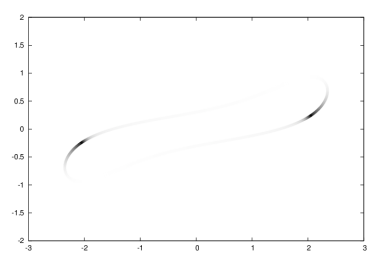
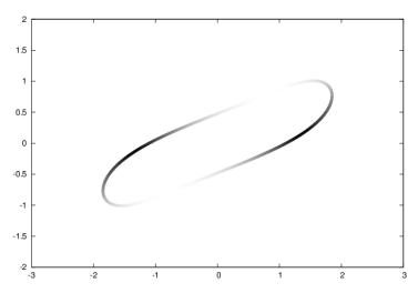
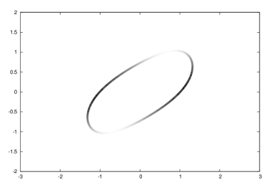
Figure 4: (2 adapt_9,4) Plots of the discrete surface mass on $\Gamma^{m}$ at time $t=12$ for $\overline{\mu}_{\Gamma}=\overline{\lambda}_{\Gamma}=0.01$ (left), $\overline{\mu}_{\Gamma}=\overline{\lambda}_{\Gamma}=1$ (middle) and $\overline{\mu}_{\Gamma}=\overline{\lambda}_{\Gamma}=10$ (right). Below are plots of the discrete surface mass against arclength.

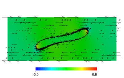
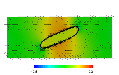
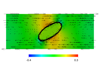
Figure 5: (2 adapt_9,4) Velocity fields for the solutions depicted in Figure 4, with the background colouring depending on the pressure values.

For very small values of $\overline{\mu}_{\Gamma}=\overline{\lambda}_{\Gamma}$ an interesting effect can be observed. As this value gets smaller, we observe a marked concentration of the discrete surface material density $\rho_{\Gamma}^{m}$ at two points on the interface. This poses a challenge for the numerical methods, as the peaks in the surface mass density lead to sharp fronts, which behave almost like a shock. We exhibit the difficulties of the schemes (4.8a–f) and (4.18a–f) with the “degenerate” case $\overline{\mu}_{\Gamma}=\overline{\lambda}_{\Gamma}=0$ in Figure 6. Clearly, the scheme (4.8a–f) displays a very nonuniform mesh, with some vertices close to coalescence. The latter appears to lead to small oscillations in $\rho_{\Gamma}^{m}$. The scheme (4.18a–f), on the other hand, shows very uniform meshes, but suffers from oscillations in the discrete surface mass density where $\rho_{\Gamma}^{m}$ is close to zero. On recalling Remark 4.5, we note that by adding numerical diffusion into the scheme, these oscillations can be avoided. This is underlined by the numerical results shown in Figure 6 for the scheme (4.18a–f) with numerical diffusion; $\vartheta(s)=\tfrac{s}{20}$.

Figure 6: (adapt_7,3) Plots of $\Gamma^{m}$ and plots of the discrete surface mass against arclength at time $t=12$ for $\overline{\mu}_{\Gamma}=\overline{\lambda}_{\Gamma}=0$ for the schemes (4.8a–f), top, (4.18a–f), middle, and (4.18a–f) with numerical diffusion; $\vartheta(s)=\tfrac{s}{20}$, bottom.

From a physical point of view it is not easy to explain the fact that the surface mass accumulates at two points on the interface. However, we recall from Theorem 3.7 that such a relocation of mass on the interface leads to a smaller overall energy, if the discrete velocity $\vec{U}^{m}$ at these points is zero, or nearly zero. In fact, this is what appears to happen for $\overline{\mu}_{\Gamma}=\overline{\lambda}_{\Gamma}=0$, as can be seen from the velocity plot in Figure 7.

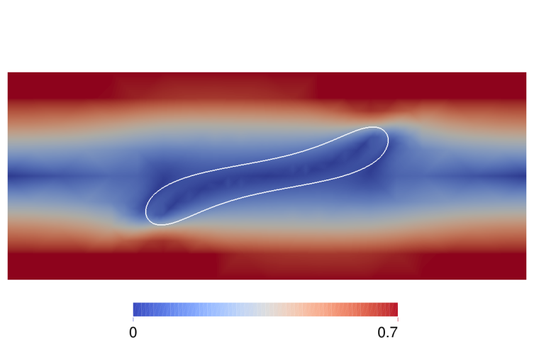
Figure 7: (adapt_7,3) A plot of $|\vec{U}^{m}|$ at time $t=12$ for $\overline{\mu}_{\Gamma}=\overline{\lambda}_{\Gamma}=0$ for the scheme (4.18a–f) with numerical diffusion; $\vartheta(s)=\tfrac{s}{20}$.

In the next simulation we consider the presence of surfactant on the interface. To this end, we choose the linear equation of state (2.19a) with $\beta=0.5$ and let

$$\mu_{\Gamma}(r)=\overline{\mu}_{\Gamma}\,(1+b_{\mu}\,[r]_{+})\quad\text{and}\quad\lambda_{\Gamma}(r)=\overline{\lambda}_{\Gamma}\,(1+b_{\lambda}\,[r]_{+})\quad\forall\ r\in{\mathbb{R}}\,,$$ (6.3)

where $\overline{\mu}_{\Gamma}=\overline{\lambda}_{\Gamma}=0.1$ and $b_{\mu}=b_{\lambda}=100$, with the remaining parameters as in (6.2). We also let $\rho_{\Gamma,0}=1$, while the initial distribution of surfactant on $\Gamma(0)$ is chosen as

$$\psi_{0}(\vec{z})=10^{-6}+[z_{1}]_{+}\,.$$ (6.4)

The evolutions of the approximations of $\psi$ and $\rho_{\Gamma}$ can be seen in Figure 8. The initially onesided distribution of surfactant, together with the definitions (6.3), leads to the bubble moving significantly to the right. The higher concentration of surfactant on the right leads to surface tension gradients on the interface, which then cause tangential shear stresses on the interface. These so called Marangoni forces lead to the overall movement of the drop to the right. Varying the value of $\beta$ between $0$ and $1$ had no significant effect on the overall evolution, and so we omit further numerical results for this setting.

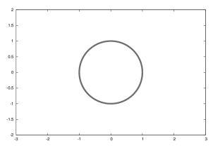
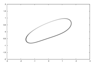
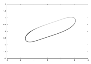
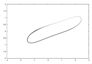
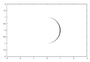
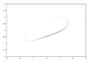
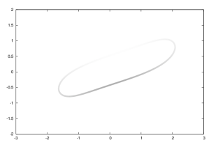
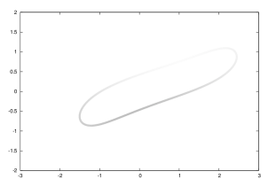
Figure 8: (2 adapt_9,4) The time evolution of a drop in shear flow with (2.19a) and $\beta=0.5$ for the scheme (4.18a–f). The top two rows show the evolution of the discrete surface material density, while the lower two rows show the evolution of the discrete surfactant concentration. Plots are at times $t=0,\,4,\,8,\,12$. In the first row the grey scales linearly with the surface material density ranging from 0 (white) to 1.4 (black). In the third row the grey scales linearly with the surfactant concentration ranging from 0 (white) to 1 (black).

6.2.2 Rising bubble

In this subsection we compare the schemes (4.8a–f) and (4.18a–f) for a rising bubble experiment that is motivated by the benchmark problems in ? for two-phase Navier–Stokes flow. In particular, we use the setup described in ?, see Figure 2 there; i.e. $\Omega=(0,1)\times(0,2)$ with $\partial_{1}\Omega=[0,1]\times\{0,2\}$ and $\partial_{2}\Omega=\{0,1\}\times(0,2)$. Moreover, $\Gamma_{0}=\{\vec{z}\in{\mathbb{R}}^{2}:|\vec{z}-(\frac{1}{2},\frac{1}{2})^{T}|=\frac{1}{4}\}$. The physical parameters from the test case 1 in ?, Table I are given by

$$\rho_{+}=1000\,,\quad\rho_{-}=100\,,\quad\mu_{+}=10\,,\quad\mu_{-}=1\,,\quad\gamma_{0}=24.5\,,\quad\vec{f}_{1}=-0.98\,\vec{e}_{d}\,,\quad\vec{f}_{2}=\vec{0}\,,$$ (6.5)

where, here and throughout, $\{\vec{e}_{j}\}_{j=1}^{d}$ denotes the standard basis in ${\mathbb{R}}^{d}$. For the surfactant problem we choose the parameters $\mathcal{D}_{\Gamma}=0.1$ and (2.19a) with $\beta=0.5$. For the surface material parameters we choose $\overline{\mu}_{\Gamma}=\overline{\lambda}_{\Gamma}=0.1$ and $\rho_{\Gamma,0}=1$. We refer to our recent papers ?? for numerical simulations for this benchmark problem in the absence of a Boussinesq–Scriven surface fluid.

We start with a simulation for the scheme (4.8a–f), using the discretization parameters adapt_7,3. The results can be seen on the left of Figure 9. We see that the vertices of the approximation $\Gamma^{m}$ are transported with the fluid flow. This means that many vertices can be found at the bottom of the bubble, with hardly any vertices left at the top.

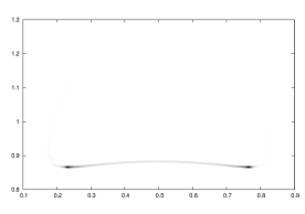
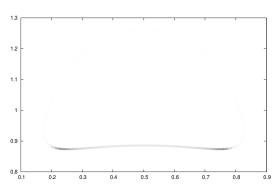
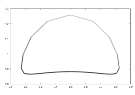
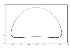
Figure 9: (adapt_7,3) Vertex distributions for the final bubble at time $t=3$ for the schemes (4.8a–f), left, and (4.18a–f), right. The latter scheme uses numerical diffusion with $\vartheta(s)=\tfrac{s}{20}$. The middle row shows the discrete surface material densities, while the bottom row shows the discrete surfactant concentrations. In the former the grey scales linearly with the surface material density ranging from 0 (white) to 9 (black), while in the latter the grey scales linearly with the surfactant concentration ranging from 0 (white) to 0.7 (black).

We also remark that for this computation the area of the inner phase decreases by $1.3\%$, so the volume of the two phases is not preserved. The same computation for our preferred scheme (4.18a–f), where the tangential movement of vertices yields an almost equidistributed approximation of $\Gamma^{m}$, can be seen on the right of Figure 9. In order to avoid oscillations in $\rho^{m}_{\Gamma}$ close to zero, we use numerical diffusion with $\vartheta(s)=\tfrac{s}{20}$ for this numerical experiment. We remark that for this computation the areas of the two phases, as well as the total surfactant amount and the total surface mass on $\Gamma^{m}$, were conserved.

In view of the superior mesh properties of our preferred scheme (4.18a–f), from now on we only consider numerical experiments for the scheme (4.18a–f).

6.3 Numerical experiments in 3d

In this subsection we present numerical results for $d=3$ for our preferred scheme (4.18a–f). As discretization parameters we always choose $\frac{1}{10}\,{\rm adapt}_{5,2}$.

6.3.1 Bubble in shear flow

In this subsection we report on some 3d analogues of the computations in §6.2.1. In particular, we perform shear flow experiments on the domain $\Omega=(-5,5)\times(-2,2)^{2}$ with $\partial\Omega=\partial_{1}\Omega$ and $\vec{g}(\vec{z})=(\frac{1}{2}\,z_{3},0,0)^{T}$. The physical parameters are as in (6.2), and for simplicity we take $\rho_{\Gamma,0}=0$. See Figure 10 for the final bubble shapes for a selection of parameters $\overline{\mu}_{\Gamma}$ and $\overline{\lambda}_{\Gamma}$ in (2.9).

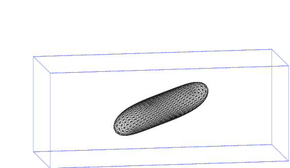
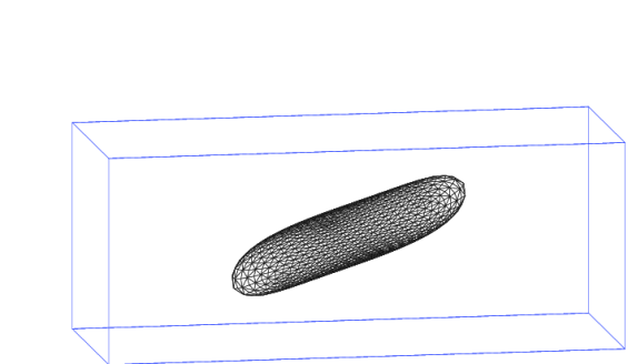
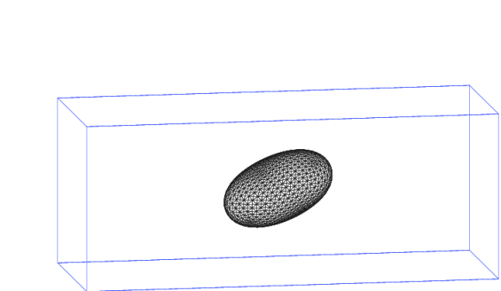
Figure 10: The discrete interface $\Gamma^{m}$ at time $t=12$ for a drop in shear flow with $\rho_{\Gamma,0}=0$ for (2.20) and (2.9) with $\overline{\mu}_{\Gamma}=\overline{\lambda}_{\Gamma}=0$, $\overline{\mu}_{\Gamma}=1$, $\overline{\lambda}_{\Gamma}=0$, $\overline{\mu}_{\Gamma}=\overline{\lambda}_{\Gamma}=1$, $\overline{\mu}_{\Gamma}=0$, $\overline{\lambda}_{\Gamma}=1$ (clockwise from top left).

6.3.2 Rising bubble

Here we consider the natural 3d analogue of the problem in §6.2.2. To this end, we let $\Omega=(0,1)\times(0,1)\times(0.2)$ with $\partial_{1}\Omega=[0,1]\times[0,1]\times\{0,2\}$ and $\partial_{2}\Omega=\partial\Omega\setminus\partial_{1}\Omega$. Moreover, we set $T=3$, $\Gamma_{0}=\{\vec{z}\in{\mathbb{R}}^{3}:|\vec{z}-(\frac{1}{2},\frac{1}{2},\frac{1}{2})^{T}|=\frac{1}{4}\}$, and choose all the remaining parameters as in §6.2.2; recall e.g. (6.5). As in the 2d equivalent, the bubble rises due to density difference against the direction of gravity. In the process, the surfactant and the surface mass accumulate at the bottom of the bubble. We show the concentrations of these two quantities in Figure 11.

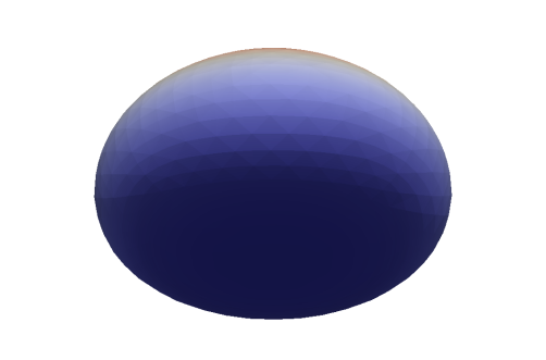
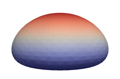
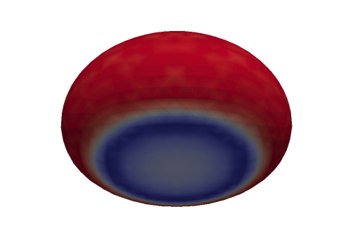
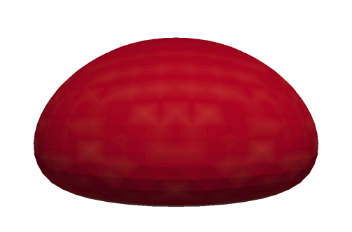
Figure 11: The surfactant concentration $\Psi^{m}$ and the surface mass $\rho^{m}_{\Gamma}$ on $\Gamma^{m}$ at time $t=3$. The top row shows $\Psi^{m}$, with the colour ranging from red (0.3) to blue (0.6). The bottom row shows $\rho^{m}_{\Gamma}$, with the colour ranging from red (0) to blue (6.5).