Quantum-mechanical calculation of ionization potential lowering in dense plasmas

Abstract

The charged environment within a dense plasma leads to the phenomenon of ionization potential depression (IPD) for ions embedded in the plasma. Accurate predictions of the IPD effect are of crucial importance for modeling atomic processes occurring within dense plasmas. Several theoretical models have been developed to describe the IPD effect, with frequently discrepant predictions. Only recently, first experiments on IPD in Al plasma have been performed with an x-ray free-electron laser (XFEL), where their results were found to be in disagreement with the widely-used IPD model by Stewart and Pyatt. Another experiment on Al, at the Orion laser, showed disagreement with the model by Ecker and Kröll. This controversy shows a strong need for a rigorous and consistent theoretical approach to calculate the IPD effect. Here we propose such an approach: a two-step Hartree-Fock-Slater model. With this parameter-free model we can accurately and efficiently describe the experimental Al data and validate the accuracy of standard IPD models. Our model can be a useful tool for calculating atomic properties within dense plasmas with wide-ranging applications to studies on warm dense matter, shock experiments, planetary science, inertial confinement fusion and studies of non-equilibrium plasmas created with XFELs.

I Introduction

The dense plasma state is a common phase of matter in the universe and can be found in all types of stars Taylor (1994) and within giant planets Chabrier (2009); Helled et al. (2011). Dense plasmas are commonly created during experiments involving high-power light sources such as, e.g., the National Ignition Facility Moses et al. (2009), and recently developed x-ray free-electron lasers (XFELs) LCLS Emma et al. (2010) and SACLA Ishikawa and Ueda (2012). In dense plasmas, free electrons stay in the close vicinity of ions. The ions then cannot any longer be treated as isolated species, as the screening by the dense environment shifts their atomic energy levels, leading to a reduction of the ionization potentials. This effect is known as ionization potential depression (IPD). Quantitative predictions of this effect are of crucial importance for a correct understanding and accurate modeling of any atomic processes occurring within a dense plasma environment WDM (2012), i.e., for studies on warm dense matter Glenzer and Redmer (2009); Drake (2009), shock experiments Lee et al. (2009); García Saiz et al. (2008), planetary science Knudson et al. (2012); Nettelmann et al. (2008), inertial confinement fusion Glenzer et al. (2010); Lindl (1995) and studies of non-equilibrium plasmas created with XFELs Corkum (2008); Fäustlin et al. (2010). Several theoretical models have been developed to describe the IPD effect. An early development was the model proposed by Ecker and Kröll (EK) Ecker and Kröll (1963) for strongly coupled plasma, later extended to the weakly coupled regime by Stewart and Pyatt (SP) Stewart and Pyatt (1966) (for more examples, see Ref. Murillo and Weisheit (1998)). However, until recently there were no experimental data available to verify the accuracy of these models whose predictions sometimes differed extensively.

First experiments on the screening effect of plasma on atoms embedded in the plasma have been performed at LCLS Vinko et al. (2012); Ciricosta et al. (2012); Cho et al. (2012). XFELs provide radiation of extremely high peak brightness and pulse duration shorter or comparable with the characteristic times of the electron and ion dynamics within irradiated systems. The dense electronic systems can quickly thermalize via electron–electron collisions and impact ionization processes Fäustlin et al. (2010). Because of the ultrashort pulse duration (typically tens of femtoseconds), only a thermalized electron plasma is probed while the ions still remain cold. This provides access to the properties of a solid-density material at temperature of $10^{5}$–$10^{6}$ K ($\approx 10$–100 eV). Specifically, the experiments in Refs. Vinko et al. (2012); Ciricosta et al. (2012); Cho et al. (2012) measured $K$-edge thresholds and $K\alpha$ emission from solid-density aluminum (Al) plasma. They have been followed by another experiment at the high-power Orion laser Hoarty et al. (2013a, b). This experiment investigated $K$-shell emissions from hot dense Al plasma. Both experimental teams tried to describe their findings with the EK and SP models. In the first experiment a disagreement of the measured $K$-edges with the extensively used SP model was claimed. A modified EK model was proposed to fit the experimental data Ciricosta et al. (2012); Preston et al. (2013). However, the data from the experiment on hot dense Al plasma Hoarty et al. (2013a) could only be described with the SP model. The EK model was found to be in clear disagreement with these data.

This controversy shows a strong need for a rigorous and consistent theoretical approach able to calculate the IPD effect for plasmas in different coupling regimes. Here we propose such an approach: a two-step Hartree-Fock-Slater (HFS) method. This model derives the electronic structure of an ion embedded in the electron plasma from the finite-temperature approach Mermin (1963), assuming thermalization of bound electrons within the free-electron plasma. It can also treat individual electronic configurations of plasma ions, which enables a description of discrete transitions. In this paper, we demonstrate that this model successfully describes laser-irradiated Al solids under the conditions of the LCLS Vinko et al. (2012); Ciricosta et al. (2012); Cho et al. (2012) and Orion laser Hoarty et al. (2013a, b) experiments. Furthermore, we gain an improved understanding of the validity of the widely-used EK and SP models.

II Two-step Hartree-Fock-Slater model

In the first step, we apply the thermal HFS approach for a given finite temperature. Here we assume that the electrons are fully thermalized. In general, XFEL radiation induces non-equilibrium dynamics of electrons, for instance, in carbon-based materials exposed to hard X-rays Hau-Riege (2013). For the solid-density Al plasma studied in the recent experiment Vinko et al. (2012), the incident photon energy is near the ionization threshold, ejecting electrons with low kinetic energy. Due to the high density and low kinetic energy, electron cross sections are large, so that electrons equilibrate rapidly within the ultrashort pulse duration. For example, in the Al plasma considered here, the energy of a photoelectron is less than 270 eV and the highest energy of an Auger electron is about 1.4 keV. With a kinetic energy in this regime, the estimated time scale of electron thermalization is a few femtoseconds for diamond Ziaja et al. (2005) and is expected to be shorter for solid Al due to higher impact ionization cross sections. Therefore, we assume that the electrons are thermalized within the pulse duration of tens of femtoseconds.

The standard Hartree-Fock and Hartree-Fock-Slater (HFS) approaches Slater (1951); Herman and Skillman (1963) treat electronic structure at zero temperature ($T=$0 eV). They use the Ritz variational principle for the ground-state energy. Recently, Thiele et al. Thiele et al. (2012) proposed an extension of the standard HFS model, including plasma environment effects through the Debye screening (see also Refs. Saha et al. (2002); Mukherjee et al. (2002); Das et al. (2011)). However, this model is not applicable to plasmas with low temperature, where the Debye screening approximation breaks down Murillo and Weisheit (1998). Also, it is intrinsically inconsistent to combine the $T=0$ eV approach with Debye screening for a plasma with a non-zero electron temperature. To overcome this inconsistency, the electronic structure has to be derived from a finite-temperature approach. Such a finite-temperature Hartree-Fock approach was proposed by Mermin (1963).

Here we use the average-atom model Rozsnyai (1972), which is a variant of the finite-temperature approach. Basically, it predicts average orbital properties and occupation numbers at a given temperature. There have been various implementations of the average-atom approach. Depending on their treatment of the electronic structure of atoms, they can be categorized as quantum mechanical approaches, such as the Hartree-Fock-Slater (HFS) method or local density approximation (LDA) Rozsnyai (1972); Liberman (1979); Blenski and Ishikawa (1995); Johnson et al. (2006); Sahoo et al. (2008); Johnson et al. (2012); Cauble et al. (1984); Davis and Blaha (1990); Piron and Blenski (2011); Starrett and Saumon (2013); Pain et al. (2006a, b), or semi-classical approaches, such as the Thomas-Fermi (TF) method Feynman et al. (1949); Rozsnyai (1972); Crowley (1990); Yuan (2002). There are also implementations with simplified super-configurations Blenski et al. (1997a, b); Faussurier (1999); Pain et al. (2006a, b) and with the screened hydrogenic model More (1982); Faussurier et al. (1997a, b); Faussurier (1999). The atomic potential within a plasma is usually based on the muffin-tin approximation Liberman (1979); Blenski and Ishikawa (1995); Johnson et al. (2006); Sahoo et al. (2008); Johnson et al. (2012); Rozsnyai (1972); Yuan (2002) or an extended model including ion–ion correlation Cauble et al. (1984); Davis and Blaha (1990); Crowley (1990); Starrett and Saumon (2013). These average-atom models have been applied to calculate physical quantities within plasmas, such as lowering of the ionization energy Davis and Blaha (1990), photoabsorption processes Blenski et al. (1997a); Johnson et al. (2006), and scattering processes Johnson et al. (2012, 2013). Our average-atom implementation presented here is based on the quantum mechanical approach with the muffin-tin approximation Blenski and Ishikawa (1995); Johnson et al. (2006); Sahoo et al. (2008); Johnson et al. (2012), but it benefits from a numerical grid technique, which will be discussed in detail later.

The major distinction of our proposed method from previous average-atom models is not only the different numerical method. In this paper, we will develop a simple model to retrieve more complete information from the average-atom approach. We propose a two-step model: an average-atom calculation as the first step and a fixed-configuration calculation as the second step. From the average-atom approach, we obtain a grand-canonical ensemble at a given temperature with a simple electronic mean field associated with all possible configurations. Using this information, we then calculate improved mean fields for selected configurations of interest. Note that our two-step model is relatively inexpensive, in comparison with polyatomic density-functional calculations, and is easily applicable to any atomic species. This two-step model is described in detail in the three following subsections.

II.1 Hartree-Fock-Slater calculation with a muffin-tin-type potential

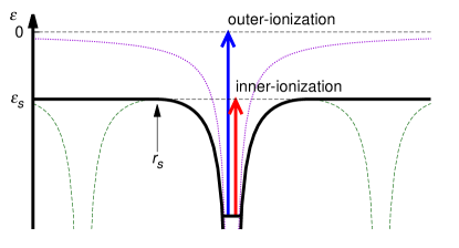
Figure 1: Schematic diagram of an atomic model in a solid or a plasma. The purple dotted curve is the isolated atomic potential, the green dashed curve is the crystalline potential, and the black thick curve is the muffin-tin-type potential. The muffin-tin flat potential is denoted as $\varepsilon_{s}$ and the Wigner-Seitz radius is $r_{s}$.

To describe the electronic structure in a solid or a plasma, we employ a muffin-tin-type potential Slater (1937) as depicted in Fig. 1. Influenced by the free electrons and neighboring ions, the atomic potential is lowered in comparison to that in an isolated atom. The sphere surrounding an atom is defined by the Wigner-Seitz radius, $r_{s}$. If the solid consists of a single atomic species, then $r_{s}=(3/4\pi n_{i})^{1/3}$, where $n_{i}$ is the number density of ions in the solid. Here we assume that the positions of the ions are fixed. Therefore the Wigner-Seitz radius does not change during the calculation. We assume charge neutrality such that the ionic charge density outside the Wigner-Seitz sphere is compensated by the electron density. The net charge inside the Wigner-Seitz sphere is also zero on average, so that the potential outside is constant. We use this muffin-tin-type model for all our calculations.

Our implementation of the muffin-tin potential differs from the original model suggested by Slater Slater (1937) and its quantum-mechanical implementations Blenski and Ishikawa (1995); Johnson et al. (2006); Sahoo et al. (2008); Johnson et al. (2012). First, the constant potential outside the atomic sphere is self-consistently calculated in our model, whereas it is set to zero in other previous implementations Slater (1937); Blenski and Ishikawa (1995); Johnson et al. (2006); Sahoo et al. (2008); Johnson et al. (2012). We refer to this constant potential as the muffin-tin flat potential, $\varepsilon_{s}$. Second, we calculate both bound- and continuum-state wave functions with the same atomic potential, using numerical grids with a sufficiently large radius far from $r_{s}$. This makes our method distinct from other implementations where a continuum state outside $r_{s}$ is usually given as a plane wave and special boundary conditions for both bound and continuum states are required.

With the muffin-tin flat potential, we may consider different ionization processes in a solid or a cluster Last and Jortner (1999); Krainov and Smirnov (2002). The ionization energy is defined as the energy needed to transfer an electron to the continuum level located at $\varepsilon=0$, which corresponds to the binding energy measured with photoelectron spectroscopy. In a solid or a cluster, this process would be called outer-ionization. On the other hand, there is already a continuum of states starting at $\varepsilon_{s}$, when the muffin-tin-type potential is imposed. It defines excitation into the continuum for $\varepsilon_{s}\leq\varepsilon\leq 0$, which would be called inner-ionization. In metals like aluminum, the conduction band can be described by this continuum above $\varepsilon_{s}$ and inner-ionization is a transfer of an electron bound to an atom (narrow band) into the conduction band. Figure 1 depicts schematically outer-ionization and inner-ionization processes for the muffin-tin-type potential.

We solve the effective single-electron Schrödinger equation with the muffin-tin-type potential (atomic units are used unless specified otherwise),

$$\left[-\frac{1}{2}\nabla^{2}+V(\mathbf{r})\right]\psi(\mathbf{r})=\varepsilon\psi(\mathbf{r}),$$ (1)

where the potential is the Hartree-Fock-Slater (HFS) potential inside $r_{s}$ and is constant outside $r_{s}$,

$$V(\mathbf{r})=\begin{cases}{\displaystyle-\frac{Z}{r}+\int_{r^{\prime}\leq r_{s}}d^{3}r^{\prime}\;\frac{\rho(\mathbf{r}^{\prime})}{|\mathbf{r}-\mathbf{r}^{\prime}|}+V_{\text{x}}[\rho(\mathbf{r})]}&\text{for }r\leq r_{s},\\ {\displaystyle V(r_{s})}&\text{for }r>r_{s},\end{cases}$$ (2)

where $Z$ is the nuclear charge, $\rho(\mathbf{r})$ is the electronic density, and $V_{\text{x}}$ is the Slater exchange potential,

$$V_{\text{x}}[\rho(\mathbf{r})]=-\frac{3}{2}\left[\frac{3}{\pi}\rho(\mathbf{r})\right]^{1/3}.$$ (3)

We use a spherically symmetric electronic density, $\rho(\mathbf{r})\rightarrow\rho(r)$, so $V(\mathbf{r})$ is also spherically symmetric. The potential for $r>r_{s}$ is given by the constant value of $V(r_{s})$, fulfilling the continuity condition at the boundary $r=r_{s}$. This constant potential defines the muffin-tin flat potential, $\varepsilon_{s}=V(r_{s})$.

For an isolated atom without the plasma, we use the original HFS potential, which is Eq. (2) without applying the Wigner-Seitz radius and the muffin-tin flat potential,

$$V_{\text{atom}}(\mathbf{r})={\displaystyle-\frac{Z}{r}+\int d^{3}r^{\prime}\;\frac{\rho(\mathbf{r}^{\prime})}{|\mathbf{r}-\mathbf{r}^{\prime}|}+V_{\text{x}}[\rho(\mathbf{r})]}.$$ (4)

In contrast to plasmas and solids, the long-range potential in the isolated atom is governed by the Coulomb potential [$=-(Q+1)/r$] where $Q$ is the charge of the atomic system. However, it is well known that the original HFS potential does not have this proper asymptotic behavior due to the self-interaction term Parr and Yang (1989). To obtain the proper long-range potential for both occupied and unoccupied orbitals, we apply the Latter tail correction Latter (1955). Thus, the unscreened HFS potential for an isolated atom is given by Eq. (4) and replaced by $-(Q+1)/r$ only when $V_{\text{atom}}(\mathbf{r})>-(Q+1)/r$.

The orbital wave function $\psi(\mathbf{r})$ is expressed in terms of the product of a radial wave function and a spherical harmonic,

$$\psi_{nlm}(\mathbf{r})=\frac{u_{nl}(r)}{r}Y^{m}_{l}(\theta,\phi),$$ (5)

where $n$, $l$, and $m$ are the principal quantum number, the orbital angular momentum quantum number, and the associated projection quantum number, respectively. The radial wave function $u_{nl}(r)$ is solved by the generalized pseudospectral method Yao and Chu (1993); Tong and Chu (1997). Plugging Eq. (5) into Eq. (1), we obtain the radial Schrödingier equation for a given $l$,

$$\left[-\frac{1}{2}\frac{d^{2}}{dr^{2}}+\frac{l(l+1)}{2r^{2}}+V(r)\right]u_{nl}(r)=\varepsilon_{nl}u_{nl}(r).$$ (6)

The Hamiltonian and radial wave function in Eq. (6) are discretized on a nonuniform grid for $0\leq r\leq r_{\text{max}}$. Note that the boundary conditions are $u_{nl}(0)=u_{nl}(r_{\text{max}})=0$, and no additional boundary condition at $r_{s}$ is imposed. After diagonalizing the discretized Hamiltonian matrix, one obtains not only bound states ($\varepsilon<\varepsilon_{s}$) but also a discretized pseudocontinuum ($\varepsilon\geq\varepsilon_{s}$). With a sufficiently large radius $r_{\text{max}}$, the distribution of these pseudocontinuum states becomes dense enough to imitate continuum states Chu and Reinhardt (1977); Santra and Cederbaum (2002); Chu and Telnov (2004).

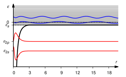
Figure 2: Plots of bound- and continuum-state energies of Al at zero temperature, obtained by diagonalization of the discretized Hamiltonian matrix. Some of bound- and continuum-state wave functions are also plotted. The maximum radius is $r_{\text{max}}=100$ a.u. used in the calculation.

Figure 2 shows some pseudocontinuum states as well as bound states ($2s$ and $2p$) of Al at zero temperature. The dense horizontal lines above $\varepsilon_{s}$ are all pseudocontinuum states. Here we use $r_{\text{max}}=100$ a.u., which is much larger than $r_{s}=2.99$ a.u. from the Al solid density (2.7 g/cm³). The number of grid points for $r$ is 200 and the number of partial waves is 31 ($0\leq l\leq 30)$. With these computational parameters, we obtain 6200 radial eigenstates. In the metallic Al case, only 3 states ($1s$, $2s$, and $2p$) are bound states. All other eigenstates constitute a pseudocontinuum. We keep these computational parameters for all calculations throughout the paper.

The numerical grid technique we use here attains advantageous simplicity in continuum-state calculations. One can transform the integration over positive energy into a summation over discrete states. There is no separation of the inside and outside regions, and therefore, no boundary condition at the Wigner-Seitz radius is needed. In contrast, other implementations of the muffin-tin model involve special boundary conditions at $r_{s}$. For example, Johnson et al. (2006, 2012) used the condition that the wave functions in the inner sphere are continuously connected to those in the outside region, and Sahoo et al. (2008) enforced the derivative of the wave function to vanish at the Wigner-Seitz radius. Note that different boundary conditions at $r_{s}$ lead to different electronic structures as pointed out in Ref. Johnson et al. (2012).

II.2 The first step: average-atom calculation

The first step of our two-step HFS approach is an average-atom model calculation with the muffin-tin-type potential in Eq. (2). We treat the electronic system using a grand-canonical ensemble at a finite temperature $T$ (in units of energy). The electronic density $\rho(\mathbf{r},T)$ is then constructed by

$$\rho(\mathbf{r},T) =\sum_{p}\left|\psi_{p}(\mathbf{r})\right|^{2}\tilde{n}_{p}(\mu,T),$$ (7)

where $p$ indicates the one-particle state index, i.e., $p=(n,l,m,m_{s})$ where $m_{s}$ is the spin quantum number, and $p$ runs over all bound and continuum states. Here $\{\tilde{n}_{p}(\mu,T)\}$ are fractional occupation numbers according to the Fermi-Dirac distribution with a chemical potential $\mu$,

$$\tilde{n}_{p}(\mu,T)=\frac{1}{e^{(\varepsilon_{p}-\mu)/T}+1},$$ (8)

where $\varepsilon_{p}$ is the orbital energy for a given spin-orbital $p$. The average number of electrons, $N_{\text{elec}}$, within the Wigner-Seitz sphere,

$$N_{\text{elec}}=\int_{r\leq r_{s}}d^{3}r\;\rho(\mathbf{r},T),$$ (9)

is fixed to $N_{\text{elec}}=Z$ to ensure charge neutrality. This condition serves as a constraint to determine the chemical potential at the given temperature Johnson et al. (2006); Sahoo et al. (2008); Johnson et al. (2012). In order to determine $\mu$, one must find the root of the following equation,

$$N_{\text{elec}}-\sum_{p}\left(\int_{r\leq r_{s}}d^{3}r\;\left|\psi_{p}(\mathbf{r})\right|^{2}\right)\tilde{n}_{p}(\mu,T)=0.$$ (10)

With $\mu$ obtained from Eq. (10), $\rho(\mathbf{r},T)$ is constructed from Eq. (7). With $\rho(\mathbf{r},T)$, the updated atomic potential, as well as $\varepsilon_{s}$, is obtained from Eq. (2). Then, orbitals $\{\psi_{p}(\mathbf{r})\}$ and orbital energies $\{\varepsilon_{p}\}$ are calculated, using the new potential. Again, a new $\mu$ is obtained from Eq. (10). This self-consistent field (SCF) procedure is performed until the results converge. Note that there are only three input parameters in the calculation: element species ($Z$), temperature ($T$), and solid density via the Wigner-Seitz radius ($r_{s}$). All other quantities such as orbitals, orbital energies, $\rho$, $\mu$, and $\varepsilon_{s}$ are determined self-consistently.

Regarding the exchange potential at a finite temperature, various implementations have been proposed Rozsnyai (1972); Shalitin (1973); Perrot and Dharma-wardana (1984); Pittalis et al. (2011); Karasiev et al. (2012); Pribram-Jones et al. (2014), but no unanimous expression has been identified. Perrot and Dharma-wardana (1984) proposed a parameterization of the thermal exchange potential based on the local density approximation (LDA). Rozsnyai (1972) proposed an interpolation between the zero-temperature Slater potential and the high temperature limit. In the present calculations, we use the same potential as used in the zero-temperature calculation given by Eq. (3). Note that our approach can be easily combined with any type of exchange potential. We will discuss the dependence on different thermal exchange potentials in Sec. III.

II.3 The second step: fixed-configuration calculation

The second step in our two-step HFS approach is a fixed configuration calculation for bound electrons in the presence of the free-electron density. Within the average-atom model, one cannot obtain orbital energies of individual electronic configurations associated with different charge states. Instead, orbital energies in the average-atom model represent averaged quantities for an averaged configuration with fractional occupational numbers. However, in a fluorescence experiment, for instance, one can see discrete transition lines corresponding to individual charge states Vinko et al. (2012), which are not accessible within the average-atom model. In order to describe individual electronic configurations within a plasma environment, we propose a fixed-configuration scheme.

With the grand-canonical ensemble, one can calculate the probability distribution Pei and Chang (2000) of all possible bound-state configurations (see Appendix A for details),

$$P_{[n_{b}]}=\prod_{b}^{\text{bound}}\frac{e^{-(\varepsilon_{b}-\mu)n_{b}/T}}{1+e^{-(\varepsilon_{b}-\mu)/T}},$$ (11)

where $[n_{b}]=(n_{1},\cdots,n_{B})$ indicates the fixed bound-state configuration, and $B$ is the number of bound one-electron states. Here $b$ runs over all bound states $(1\leq b\leq B)$ and $n_{b}$ is an integer occupation number (0 or 1) in the bound-electron configuration. The probability of finding the charge state $Q$ is given by the sum of all associated bound-state configurations,

$$P_{Q}=\sum_{[n_{b}]}^{Q}P_{[n_{b}]}.$$ (12)

Here $[n_{b}]$ runs over all possible bound-state configurations satisfying $\sum_{b}^{\text{bound}}n_{b}=Z-Q$.

From the probability distributions in Eqs. (11) and (12), one can choose one bound-electron configuration from the grand-canonical ensemble and perform a single SCF calculation with this fixed configuration. For example, it is possible to choose the most probable configuration associated with the most probable charge state. The $K\alpha$ transition energy calculated from this configuration gives one discrete line in the x-ray emission spectrum. Different configurations contribute to different transition lines, so measurement of these lines maps out the distribution of all possible configurations and charge states.

Here we focus on individual bound-electron configurations. Even though the bound-state electronic structure is influenced by the presence of the plasma electrons, we assume that it is not sensitive to detailed free-electron configurations in the plasma. Therefore, once we choose one bound-electron configuration, we calculate the free-electron density as an average of all possible free-electron configurations for the given bound-electron configuration (see Appendix B),

$$\rho_{f}(\mathbf{r},T)=\sum_{p}^{\text{continuum}}\left|\psi_{p}(\mathbf{r})\right|^{2}\tilde{n}_{p}(\mu,T),$$ (13)

which turns out to be independent of the bound-electron configuration selected. This free-electron density is self-consistently obtained in the first step and is kept fixed in the second step. The bound-electron density is constructed with a fixed electron configuration,

$$\rho_{b}(\mathbf{r})=\sum_{b}^{\text{bound}}\left|\psi_{b}(\mathbf{r})\right|^{2}n_{b}.$$ (14)

Then, the total electron density is constructed as the sum of the bound and free-electron densities,

$$\rho(\mathbf{r})=\rho_{b}(\mathbf{r})+\rho_{f}(\mathbf{r},T).$$ (15)

With this total electron density, we perform a HFS calculation using a microcanonical ensemble. In this case, $\rho_{b}$ is self-consistently updated, whereas $\rho_{f}$ remains fixed during the SCF procedure. This approach allows the bound electrons in a given configuration to adjust to the presence of the plasma electrons.

III Applications of two-step HFS model to Al plasmas

In this section, we apply the two-step HFS model to laser-irradiated Al solid Vinko et al. (2012); Ciricosta et al. (2012); Hoarty et al. (2013a). The two-step procedure is carried out as follows. First, we perform a finite-temperature HFS calculation to determine the temperature needed to achieve a certain average charge state within the plasma. We then use the free-electron density $\rho_{f}(\mathbf{r},T)$ obtained from the finite-temperature calculation to perform a fixed-configuration HFS calculation for the given charge state to determine the energy of the $1s$ orbital and the energy of the energetically lowest $p$ orbital above $2p$ (always referred to as $3p$, whether it is bound or not). Both the first and second steps of our two-step HFS model are implemented as an extension of the xatom toolkit Son and Santra (2011); Son et al. (2011), which can calculate any atomic element and any electronic configuration within a non-relativistic framework. All calculations are performed with the computational parameters stated in Sec. II.2 and are fully converged.

III.1 Al plasmas at low temperature calculated in the first step

Table 1: Electronic structure of Al metal and Al plasma. All energies in our present calculations are subtracted by $\varepsilon_{s}$, in order to compare with other theoretical data. Al solid density is $n_{i}^{\circ}=2.7$ g/cm³ and $\bar{Q}$ is the average charge state. Energies are in eV.

	$T=10$ eV, $n_{i}=n_{i}^{\circ}$		$T=5$ eV, $n_{i}=0.1n_{i}^{\circ}$
Level	Present	Ref. Sahoo et al. (2008)	Present	Ref. Johnson et al. (2006)
$1s$	$-1530.1$	$-1495.0$	$-1547.3$	$-1501.8$
$2s$	$-102.5$	$-101.2$	$-119.6$	$-108.3$
$2p$	$-64.9$	$-63.9$	$-82.0$	$-71.0$
$3s$	–	$-6.3$	$-8.6$	$-7.0$
$3p$	–	–	$-2.5$	$-1.5$
$\mu$	$-1.5$	–	$-11.1$	$-10.4$
$\bar{Q}$	$+3.01$	$+2.38$	$+1.34$	$+1.49$

In order to benchmark our calculations, we apply our average-atom model (the first step of our two-step approach) to Al solid ($T=0$ eV) and low-temperature Al plasma ($T\leq 10$ eV). In our average-atom model, we self-consistently determine all orbital energies, the muffin-tin flat potential, and the chemical potential. The Fermi level is the position of the chemical potential $\mu$ at $T=0$ eV. The muffin-tin flat potential $\varepsilon_{s}$ represents the lower limit of the delocalized states, corresponding to the lowest occupied state in the conduction band. Therefore, if one defines the Fermi energy relative to the beginning of the conduction band, it is given by $\varepsilon_{F}=\mu-\varepsilon_{s}$ in our calculation. For $T>0$ eV, the $K$-shell inner-ionization energy is defined by the difference between the muffin-tin flat potential and the $1s$ orbital energy, $E_{K}=\varepsilon_{s}-\varepsilon_{1s}$, employing the zeroth-order approximation for the HFS energy, which is similar to Koopmans’ theorem for the Hartree-Fock method. For the Al solid at $T=0$ eV, the inner-ionization energy is given by $E_{K}=\mu-\varepsilon_{1s}$, because orbitals below the Fermi level are fully occupied and there are no transitions into those orbitals. As the temperature increases, the chemical potential becomes lower than the muffin-tin flat potential and the occupation numbers in the continuum states follow the thermal Boltzmann distribution for the given plasma temperature. For instance, the occupation number in $3s$ and $3p$ is $\sim$0.46 at $T=10$ eV and $\sim$0.18 at $T=30$ eV. In this way, for $T>0$ eV the continuum states above the muffin-tin flat potential become available for electronic transitions.

Taking into account the HFS approximation and the muffin-tin approximation, our calculations provide reasonable electronic structures for metallic states. For Al at $T=0$ eV and solid density (2.7 g/cm³), the average charge $\bar{Q}$ is $+3$, indicating that only 10 electrons are bound as $1s^{2}$, $2s^{2}$, and $2p^{6}$. The other 3 electrons, which would be $3s^{2}$$3p^{1}$ in an isolated atom, are then already in the continuum, i.e., within the conduction band. Therefore, our model can mimic the electronic structure of the metal. With our method, we found $\varepsilon_{F}=8.0$ eV. The experimental Fermi energy is 11.7 eV Ashcroft and Mermin (1976). Our method calculates $E_{K}=1538.1$ eV at $T=0$ eV, while the experimental binding energy of the $K$-shell relative to the Fermi level is 1559.6 eV Thompson and Vaughan (2001).

For $T>0$ eV, Table 1 compares our results with available theoretical data. All energies in our calculations are subtracted by $\varepsilon_{s}$ in order to compare with previous calculations Johnson et al. (2006); Sahoo et al. (2008) where $\varepsilon_{s}$ is set to zero. We found that for $T\leq 10$ eV at solid density the average charge of Al is $+3$, and $M$-shells ($3s$ and $3p$) are not bound. Our finding agrees with the comment in Ref. Johnson et al. (2012), but disagrees with the results in Ref. Sahoo et al. (2008), where $3s$ is bound in this low temperature regime. In Table 1, we list energy levels of the Al plasma at $T=10$ eV in comparison with Ref. Sahoo et al. (2008). The different prediction for $M$-shell binding is ascribed to the different boundary condition as discussed in Ref. Johnson et al. (2012). At $T=5$ eV and density of 0.27 g/cm³, we compare our results with Ref. Johnson et al. (2006). The discrepancy in this case is entirely due to the different exchange potential. If we use the same LDA potential as used in Ref. Johnson et al. (2006) ($V_{\text{x}}^{\text{LDA}}=\frac{2}{3}V_{\text{x}}$), then we obtain the same results for all energy levels and the averaged charge state.

III.2 Connection between the first and second steps: bound-electron configuration and free-electron density

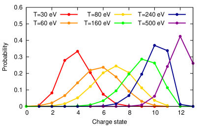
Figure 3: Probability distribution of charge states for different temperatures calculated in the first step of our two-step HFS model.

Table 2: Probability distribution of bound-electron configurations at $T=80$ eV. Configurations are listed when their probability is greater than 0.01, and the probability is calculated from the first step. $K$-shell ionization energy ($E_{K}$) and $K\alpha$ transition energy ($E_{K\alpha}$) are calculated from the second step of our two-step HFS model. $E_{K}$ and $E_{K\alpha}$ are in eV.

$Q$	Configuration	Probability	$E_{K}$	$E_{K\alpha}$
+5	$1s^{2}2s^{1}2p^{4}3s^{0}3p^{1}$	0.0193	1618.3	1497.7
	$1s^{2}2s^{2}2p^{3}3s^{0}3p^{1}$	0.0187	1623.1	1500.3
	$1s^{2}2s^{2}2p^{4}3s^{0}3p^{0}$	0.0174	1578.7	1486.7
+6	$1s^{2}2s^{1}2p^{3}3s^{0}3p^{1}$	0.0376	1658.1	1511.6
	$1s^{2}2s^{1}2p^{4}3s^{0}3p^{0}$	0.0349	1618.3	1497.7
	$1s^{2}2s^{2}2p^{3}3s^{0}3p^{0}$	0.0339	1623.1	1500.3
	$1s^{2}2s^{2}2p^{2}3s^{0}3p^{1}$	0.0205	1663.5	1514.5
	$1s^{2}2s^{1}2p^{3}3s^{1}3p^{0}$	0.0139	1656.0	1511.3
+7	$1s^{2}2s^{1}2p^{3}3s^{0}3p^{0}$	0.0681	1666.3	1512.8
	$1s^{2}2s^{1}2p^{2}3s^{0}3p^{1}$	0.0413	1705.4	1527.8
	$1s^{2}2s^{2}2p^{2}3s^{0}3p^{0}$	0.0371	1671.9	1515.8
	$1s^{2}2s^{0}2p^{3}3s^{0}3p^{1}$	0.0189	1699.3	1524.5
	$1s^{2}2s^{0}2p^{4}3s^{0}3p^{0}$	0.0175	1660.9	1509.9
	$1s^{2}2s^{1}2p^{2}3s^{1}3p^{0}$	0.0153	1705.4	1527.9
	$1s^{2}2s^{2}2p^{1}3s^{0}3p^{1}$	0.0120	1711.7	1531.2
+8	$1s^{2}2s^{1}2p^{2}3s^{0}3p^{0}$	0.0747	1718.7	1530.0
	$1s^{2}2s^{0}2p^{3}3s^{0}3p^{0}$	0.0342	1712.3	1526.7
	$1s^{2}2s^{1}2p^{1}3s^{0}3p^{1}$	0.0241	1758.5	1546.5
	$1s^{2}2s^{2}2p^{1}3s^{0}3p^{0}$	0.0217	1725.1	1533.4
	$1s^{2}2s^{0}2p^{2}3s^{0}3p^{1}$	0.0207	1751.6	1542.9
+9	$1s^{2}2s^{1}2p^{1}3s^{0}3p^{0}$	0.0437	1775.1	1549.6
	$1s^{2}2s^{0}2p^{2}3s^{0}3p^{0}$	0.0375	1768.0	1545.9
	$1s^{2}2s^{0}2p^{1}3s^{0}3p^{1}$	0.0121	1808.2	1564.1
+10	$1s^{2}2s^{0}2p^{1}3s^{0}3p^{0}$	0.0219	1827.4	1568.1
	$1s^{2}2s^{1}2p^{0}3s^{0}3p^{0}$	0.0106	1835.2	1572.1

As discussed in Sec. II.3, we choose certain fixed configurations based on the probability distribution of charge states and bound-electron configurations. Figure 3 shows the charge state distribution for $T=30$–500 eV, calculated using Eq. (12). As $T$ increases, the charge state distribution moves toward higher charge states, resulting in higher $\bar{Q}$. From the first step, it is also possible to calculate probabilities for all possible bound-electron configurations associated with individual charge states. For example, Table 2 shows bound-electron configurations at $T=80$ eV, whose probability is greater than 0.01, calculated using Eq. (11). These probability distributions of charge states and bound-electron configurations provide detailed information about the ensemble and enable us to perform the second step of our two-step approach. In Table 2, we also list $K$-shell ionization energies ($=\varepsilon_{s}-\varepsilon_{1s}$) and $K\alpha$ transition energies ($=\varepsilon_{2p}-\varepsilon_{1s}$), calculated from the second step. Individual configurations provide different ionization energies and transition energies, which cannot be captured by averaged orbital energies from the average-atom approach only. Note that the ground-state configuration is usually not the most probable configuration for given charge states, illustrating the importance of detailed electronic structures of individual configurations. In our calculation, $3s$ and $3p$ are bound at $T=80$ eV, and they are included in the bound-electron configuration. However, those $M$-shell electrons do not considerably alter the $1s$–$2p$ transition lines. For example, $E_{K\alpha}=1512.8$ eV for Al⁷⁺ $1s^{2}2s^{1}2p^{3}$ is similar to 1511.6 eV for Al⁶⁺ $1s^{2}2s^{1}2p^{3}3p^{1}$ and 1511.3 eV for Al⁶⁺ $1s^{2}2s^{1}2p^{3}3s^{1}$ (see Table 2). To compare calculated $K\alpha$ lines with experimental results, it is plausible to assign them according to the super-configuration of $K$ and $L$-shells only, as suggested in Refs. Vinko et al. (2012); Cho et al. (2012).

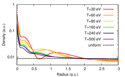
Figure 4: Free-electron density of aluminum plasma for different temperatures, obtained from the first step of our two-step model.

The free-electron density is obtained from the first step of the two-step model. Figure 4 shows the free-electron density $\rho_{f}(\mathbf{r},T)$ for different electronic temperatures ($T=30$–500 eV), calculated using Eq. (13). The density plot is normalized such that the integration of the density within $r_{s}$ yields one. This free-electron density is self-consistently optimized in the presence of the central nucleus and bound electrons, thus its distribution is highly non-uniform. As expected, the free-electron density tends to be more uniformly distributed within the Wigner-Seitz sphere at higher temperatures. For comparison, a constant and normalized density is also plotted with a dashed line in Fig. 4. The shape of the free-electron density at $T=30$ eV is attributed to the nodal structure of the $3p$ orbital in the continuum.

III.3 Ionization potential depression in Al plasmas: LCLS experiment

Table 3: Average charge state $\bar{Q}$, the most probable charge state $Q_{\text{mp}}$ and the most probable bound-electron configuration $C_{\text{mp}}$ for a given temperature $T$ from the first step of two-step HFS calculation. Note that $C_{\text{mp}}$ is the ground configuration for a given charge state, except Al⁷⁺ at $T=80$ eV.

$T$	$\bar{Q}$	$Q_{\text{mp}}$	$C_{\text{mp}}$
10	+3.01	+3	$1s^{2}2s^{2}2p^{6}$
30	+3.95	+4	$1s^{2}2s^{2}2p^{5}$
40	+4.83	+5	$1s^{2}2s^{2}2p^{4}$
60	+5.67	+6	$1s^{2}2s^{2}2p^{3}$
80	+6.87	+7	$1s^{2}2s^{1}2p^{3}$

As shown in the previous subsection, we determine from the first step for a given temperature: a) probabilities of all individual electronic configurations associated with different charge states, and b) the free-electron density. For the LCLS conditions ($T=10$–80 eV) corresponding to the strongly and moderately coupled plasma regimes, the average charge state, the most probable charge state, and the most probable configuration of this charge state are listed in Table 3.

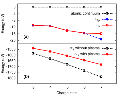
Figure 5: Energy levels as a function of the charge state for aluminum. (a) The $3p$ orbital energy and the threshold energy to the continuum ($\varepsilon_{s}$) calculated with the two-step HFS approach. The threshold energy to the continuum for isolated ions ($\varepsilon=0$) is shown for reference. (b) The $1s$ orbital energies without the plasma (unscreened HFS calculations) and with the plasma (two-step HFS calculations).

Figure 5 shows (a) the resulting $3p$ (or the lowest-energy $p$ state in the continuum) orbital energies and the muffin-tin flat potential calculated by the two-step HFS scheme with the free-electron density, and (b) the $1s$ orbital energies with and without the plasma, as a function of the charge state. All those energies are lowered as the charge state increases. Note that the $3p$ energy lies right at the threshold to the continuum, i.e., it is not bound to a single atom. The only exception is Al⁷⁺, where $3p$ lies $\sim$3.4 eV below the threshold. For an isolated atom or ion, calculated in the unscreened HFS approach, the threshold energy to the continuum is constant ($\varepsilon=0$) for all charge states. For a solid, the threshold energy to the continuum ($\varepsilon_{s}$) decreases by 5 eV from Al iv to Al viii. Lowering of the $1s$ binding energies due to the plasma environment (44–107 eV) is much larger than the lowering of the threshold energy (11–16 eV). For $T>0$ eV, the difference between the threshold energy to the continuum in Fig. 5(a) and the $1s$ orbital energy in Fig. 5(b) gives the $K$-shell ionization potential. In our approach, both the $1s$ orbital energy and the threshold energy are modified by the plasma environment.

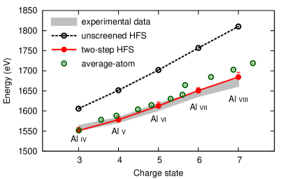
Figure 6: $K$-shell thresholds for aluminum as a function of the charge state calculated with the two-step HFS model. The experimental data are taken from Ref. Ciricosta et al. (2012). Unscreened HFS refers to calculations for isolated ions.

In the LCLS experiment on Al plasma Ciricosta et al. (2012), $K\alpha$ fluorescence was detected and spectrally resolved as a function of the incoming photon energy. In this way, the incident-photon-energy threshold for the formation of a $K$-shell hole was determined for each energetically resolvable charge state. A $K$-shell hole can be created for $T>0$ eV by inner-ionization or photo-excitation into the $3p$ orbital if $3p$ is bound. Figure 6 shows the calculated $K$-shell ionization thresholds (photo-excitation for Al⁷⁺), in comparison with the experimental results Ciricosta et al. (2012). We also plot the $K$-shell ionization thresholds for the unscreened HFS method (isolated ions) and the average-atom model. For Al⁷⁺, the resonant excitation into $3p$ is below the ionization threshold by just $\sim$3.4 eV, which may not be resolvable due to the LCLS energy bandwidth of $\sim$7 eV in experiment Vinko et al. (2012). As shown in Fig. 6, the two-step HFS calculation yields good agreement with the experimental data. However, the average-atom model alone fails in reproducing experiment, especially for high charge states. In experiment, each discrete fluorescence line selects only one charge state and the $K$-shell threshold is assigned to this specific charge state. The fixed-configuration scheme in our two-step model properly describes this selection of the $K$-shell threshold, whereas the average-atom model with the configuration averaging does not. All calculated energies were shifted by +21.5 eV, according to the difference between the inner-ionization energy calculated at $T=0$ eV (1538.1 eV) and the experimental binding energy (1559.6 eV) Thompson and Vaughan (2001). This constant energy shift is a model assumption for comparing our results to the experimental data. Note that the absolute accuracy of HFS binding energies is typically about 1%. Clearly, in order to improve the description, one would require a treatment of the electronic structure beyond the mean-field level. However, it may be anticipated that such an approach would be much less efficient than the present HFS theory. On the other hand, the error bar in the two-step HFS model in Fig. 6 indicates variation from different thermal exchange potentials used in our calculations. We have tested the thermal exchange potentials of Perrot and Dharma-wardana (1984) and Rozsnyai (1972), following the same two-step procedure as described in Sec. II, and found that the maximum deviation from the results with the zero-temperature potential is about 12 eV.

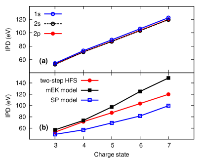
Figure 7: Plots of the ionization potential depression. (a) Comparison for all orbitals of Al calculated with the two-step HFS approach. (b) Comparison of various methods: two-step HFS model, modified EK model, and SP model. The predictions of the latter two are taken from Ref. Ciricosta et al. (2012).

By taking the difference of the ionization potentials with and without the plasma environment, we can examine the lowering of the ionization potentials not only for $K$-shell electrons but also for electrons in other subshells. For individual bound orbitals of Al ions, we obtain the IPD shown in Fig. 7(a). For isolated atoms, the ionization potential is given by $-\varepsilon^{\circ}_{j}$ where $\varepsilon^{\circ}_{j}$ is the $j$th orbital energy from the unscreened HFS calculation. For atoms in the plasma for $T>0$ eV, the inner-ionization potential is calculated by $\varepsilon_{s}-\varepsilon_{j}$, where both $\varepsilon_{s}$ and $\varepsilon_{j}$ are obtained from the two-step HFS calculation. Since the plasma screening affects each orbital differently, it is expected that IPDs for individual orbitals are different. Our results show that the IPD for $1s$ is higher than the IPD of $2s$ and $2p$ by $\sim$3 eV, but there is almost no difference in the IPDs for orbitals with the same principal quantum number ($2s$ and $2p$). This trend is similar to that observed in Ref. Thiele et al. (2012) for the Debye-screened HFS model.

Figure 7(b) depicts a comparison of various theoretical IPD models. The results of the Stewart-Pyatt (SP) model and the modified Ecker-Kröll (EK) model are taken from Ref. Ciricosta et al. (2012). The original EK model Ecker and Kröll (1963) and the SP model Stewart and Pyatt (1966) for lowering of the ionization energy have been widely used in the past decades and are implemented in several codes, e.g., flychk Chung et al. (2005) or lasnex-dca Lee (1987). Ecker and Kröll Ecker and Kröll (1963) have described lowering of the ionization potential as being due to the presence of an electric microfield. In their model, there is no difference among the IPDs of individual orbitals, and the ionization potential is considered as the difference between the ground-state energy of the charge state $Q$ and that of the charge state $(Q+1)$, which corresponds to the outermost-shell ionization potential in our calculations ($2p$ for the Al plasma). A modified version of the EK model (mEK) has been proposed in Refs. Ciricosta et al. (2012); Preston et al. (2013) by employing an empirical constant to fit the experimental data. Figure 7(b) shows that neither the mEK model nor the SP model are close to our two-step HFS approach.

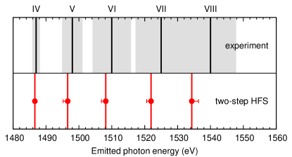
Figure 8: $K\alpha$ transition energies of aluminum ions obtained with the two-step HFS model. They are compared to the experimental data taken from Ref. Ciricosta et al. (2012). The gray areas indicate the full-width-at-half-maximum from experiment.

In Figure 8, we show the peak positions of the $K\alpha$ fluorescence lines for Al iv up to Al viii. The experimental data are taken from Ref. Ciricosta et al. (2012). The transition energies are calculated from the differences of the $2p$ and $1s$ orbital energies in the fixed-configuration scheme. The fixed bound-electron configuration associated with a given charge state is chosen from Table 3. All calculated energies are shifted by +21.5 eV, according to the difference between the Al iv transition energy calculated with the average-atom model at $T=0$ eV ($1464.9$ eV) and the experimental transition line ($1486.4$ eV) Thompson and Vaughan (2001). The error bar in the two-step HFS model shows variation from usage of different thermal exchange potentials, and the maximum deviation is about 2 eV. Our results show small deviations ($<5.7$ eV) from the experimental transition energies. Here we show transition energies for only one configuration associated with a given charge state. However, different configurations, as listed in Table 2 at $T=80$ eV, would give rise to different transition lines. For instance, the ground configuration ($1s^{2}2s^{2}2p^{2}$) of Al viii at $T=80$ eV gives a fluorescence line of +3 eV higher in energy than the most probable configuration ($1s^{2}2s^{1}2p^{3}$).

III.4 Al plasmas at high temperature and high density: Orion experiment

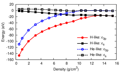
Figure 9: The muffin-tin flat potential ($\varepsilon_{s}$) and $3p$ orbital energy ($\varepsilon_{3p}$) of H-like and He-like Al as a function of the solid density at $T=700$ eV.

Our two-step scheme is applicable not only in the strongly coupled plasma regime but also in the weakly coupled plasma regime. Recently, Hoarty et al. (2013a, b) used the high-power Orion laser to create compressed Al plasmas with high temperature and measured Ly_β and He_β lines to diagnose the Al plasmas created. In Fig. 9, the two-step model calculations show that the $3p$ state of compressed Al merges with the continuum ($\varepsilon\geq\varepsilon_{s}$) as the Al density increases. The electronic temperature is 700 eV, close to the Orion experimental condition Hoarty et al. (2013a). For the bound-electron part in the second step, the H-like Al is calculated with the exact one-electron potential and the He-like Al is calculated with the exact Hartree-Fock potential. For such a high temperature, the plasma electron density contributes to only the direct Coulomb interaction Rozsnyai (1972).

When the solid density $d$ is greater than $\sim$12 g/cm³, the $3p$ state of H-like Al is no longer bound, so the Ly_β line would disappear. Likewise, the He_β line would disappear after $d>10$ g/cm³. Our results are consistent with the experimental finding of no $n=3$ transitions occurring at $d>8$–10 g/cm³. When we use different thermal exchange potentials Perrot and Dharma-wardana (1984); Rozsnyai (1972), the merging point of $3p$ becomes $\sim$8 g/cm³ and $\sim$11 g/cm³ for He_β and Ly_β, respectively. The SP model predicts delocalization of $n=3$ levels for $d>11.6$ g/cm³, whereas the EK model prediction was found to be in clear disagreement with the experimental data Hoarty et al. (2013a).

IV Conclusion

In this work, we have extended the standard HFS approach for calculating atomic energy levels for ions embedded in a plasma, taking into account plasma screening. Our two-step HFS model includes: (i) the average-atom model to obtain the free-electron density at a given temperature and (ii) the fixed-configuration model taking into account the free-electron density. Our current analysis focused on Al plasmas created by LCLS Vinko et al. (2012); Ciricosta et al. (2012) and Orion laser Hoarty et al. (2013a), covering both strongly and weakly coupled plasma regimes. Our two-step HFS results on the $K$-shell threshold energies of different charge states within Al plasma are in good agreement with the LCLS experimental data Vinko et al. (2012); Ciricosta et al. (2012). References Vinko et al. (2012); Ciricosta et al. (2012) measured fluorescence threshold energies that were then used to extract IPDs by combining the data with a specific theory model describing the unscreened ionization potentials. Thus, the estimated IPDs relied on the theory of the unscreened case, which hinders direct comparison with IPD models. In contrast, our model computes the energy shifts of all individual orbitals with and without plasma screening, thus providing IPDs in an internally consistent manner. Our calculated valence IPDs lie between the SP and mEK models. Hence, we cannot confirm that the performance of the mEK model is superior to that of the SP model, as suggested in Ref. Ciricosta et al. (2012). Moreover, in the high temperature regime, our prediction for the $3p$ state is in good agreement with the SP model and reproduces Orion experimental data Hoarty et al. (2013a). These results show that, with our proposed two-step HFS approach, a reliable and relatively inexpensive calculation of atomic properties within plasmas can be performed both for weakly and strongly coupled plasmas. We therefore expect that our model will be a useful tool for describing new data from plasma spectroscopy experiments.

Appendix A Probability distributions of charge states and configurations

The partition function of the grand-canonical ensemble for fermions is given by

$$Y =\mathrm{Tr}\{e^{-\beta(\hat{H}-\mu\hat{N})}\}$$

$$=\sum_{\{n_{p}\}}^{\text{all}}e^{-\beta\sum_{p}(\varepsilon_{p}-\mu)n_{p}}$$

$$=\prod_{p=1}^{\infty}\left(1+e^{-\beta(\varepsilon_{p}-\mu)}\right),$$ (16)

where $\beta=1/T$ is the inverse of the temperature, $\{n_{p}\}=(n_{1},n_{2},\cdots)$, and $n_{p}$ is the occupation number of the $p$th one-electron state. Here $p$ includes all bound and continuum one-electron states, and the summation runs over all possible configurations $\{n_{p}\}$. For fermions, $n_{p}$ is either 0 or 1. Then, the probability of finding one specific configuration $\{n_{p}\}$ is

$$P_{\{n_{p}\}}=\frac{1}{Y}e^{-\beta\sum_{p}(\varepsilon_{p}-\mu)n_{p}}=\prod_{p=1}^{\infty}\frac{e^{-\beta(\varepsilon_{p}-\mu)n_{p}}}{1+e^{-\beta(\varepsilon_{p}-\mu)}}.$$ (17)

Let us consider a fixed configuration, more precisely, a fixed bound-electron configuration $[n_{b}]=(n_{1},\cdots,n_{B})$, where $B$ is the number of the bound states. A general Fock-space configuration consistent with the fixed bound-electron configuration is

$$\{n_{b};n_{p^{\prime}}\}=(n_{1},\cdots,n_{B};n_{B+1},\cdots).$$ (18)

Here $n_{b}$ for $1\leq b\leq B$ is a fixed occupation number, while $n_{p^{\prime}}$ is either 0 or 1 for $p^{\prime}\geq B+1$. The probability of finding the fixed configuration $[n_{b}]$ is calculated by summing over all such configurations $\{n_{b};n_{p^{\prime}}\}$,

$$P_{[n_{b}]} =\sum_{\{n_{p}\}=\{n_{b};n_{p^{\prime}}\}}P_{\{n_{p}\}}$$

$$=\frac{1}{Y}\prod_{b=1}^{B}e^{-\beta(\varepsilon_{b}-\mu)n_{b}}\sum_{\{n_{p^{\prime}}\}}^{\text{all}}\prod_{p^{\prime}=B+1}^{\infty}e^{-\beta(\varepsilon_{p^{\prime}}-\mu)n_{p^{\prime}}}$$

$$=\frac{\prod_{b=1}^{B}e^{-\beta(\varepsilon_{b}-\mu)n_{b}}\prod_{p^{\prime}=B+1}^{\infty}\left(1+e^{-\beta(\varepsilon_{p^{\prime}}-\mu)}\right)}{\prod_{b=1}^{B}\left(1+e^{-\beta(\varepsilon_{b}-\mu)}\right)\prod_{p^{\prime}=B+1}^{\infty}\left(1+e^{-\beta(\varepsilon_{p^{\prime}}-\mu)}\right)}.$$

In the above calculation, since the occupation numbers in the bound states are fixed, they can be factored out and the remaining parts in the numerator and the denominator are canceled out. Thus, the probability reduces to

$$P_{[n_{b}]} =\prod_{b=1}^{B}\frac{e^{-\beta(\varepsilon_{b}-\mu)n_{b}}}{1+e^{-\beta(\varepsilon_{b}-\mu)}},$$ (19)

which corresponds to Eq. (11). This is for spin-orbitals $b$, i.e., $n_{b}$ is either 0 or 1. For practical purposes, we express the probability in terms of subshells,

$$P_{[n_{i}]}=\frac{\prod_{i=1}^{N_{b}}\binom{4l_{i}+2}{n_{i}}e^{-\beta(\varepsilon_{i}-\mu)n_{i}}}{\prod_{i=1}^{N_{b}}\left(1+e^{-\beta(\varepsilon_{i}-\mu)}\right)^{(4l_{i}+2)}},$$ (20)

where $i$ is the subshell index, $N_{b}$ is the number of bound subshells, and $[n_{i}]=(n_{1},\cdots,n_{N_{b}})$. For the $i$th subshell, $\varepsilon_{i}$ is the orbital energy, $l_{i}$ is the orbital angular momentum quantum number, and $n_{i}$ is the occupation number ($0\leq n_{i}\leq 4l_{i}+2$).

The probability of finding the charge state $Q$ is given by summing over all possible configurations associated with $Q$,

$$P_{Q}=\sum_{[n_{b}]}^{Q}P_{[n_{b}]}=\sum_{[n_{b}]}^{Q}\prod_{b=1}^{B}\frac{e^{-\beta(\varepsilon_{b}-\mu)n_{b}}}{1+e^{-\beta(\varepsilon_{b}-\mu)}},$$ (21)

where $[n_{b}]$ satisfies $\sum_{b=1}^{B}n_{b}=Z-Q$. This is Eq. (12). It is straightforward to verify $\sum_{Q}P_{Q}=1$. The average charge state $\bar{Q}$ is given by

$$\bar{Q} =\sum_{Q}QP_{Q}$$

$$=\sum_{Q}\sum_{[n_{b}]}^{Q}\left(Z-\sum_{p=1}^{B}n_{p}\right)\prod_{b=1}^{B}\frac{e^{-\beta(\varepsilon_{b}-\mu)n_{b}}}{1+e^{-\beta(\varepsilon_{b}-\mu)}}$$

$$=Z-\sum_{b=1}^{B}\tilde{n}_{b}(\mu,T),$$ (22)

which is used to calculate $\bar{Q}$ in Tables 1 and 3.

Appendix B Determination of free-electron density

Here we calculate the total electron density for a fixed bound-electron configuration, $[n_{b}]=(n_{1},\cdots,n_{B})$. The total density is chosen by averaging densities over all configurations $\{n_{b};n_{p^{\prime}}\}$ that have $[n_{b}]$ in common:

$$\rho_{[n_{b}]}=\sum_{\{n_{p}\}=\{n_{b};n_{p^{\prime}}\}}\rho_{\{n_{p}\}}w_{\{n_{p}\}},$$ (23)

where $w_{\{n_{p}\}}$ is a statistical weight,

$$w_{\{n_{b};n_{p^{\prime}}\}} =\frac{e^{-\beta\sum_{p}(\varepsilon_{p}-\mu)n_{p}}}{\sum_{\{n_{p}\}=\{n_{b};n_{p^{\prime}}\}}e^{-\beta\sum_{p}(\varepsilon_{p}-\mu)n_{p}}}$$

$$=\prod_{p^{\prime}=B+1}^{\infty}\frac{e^{-\beta(\varepsilon_{p^{\prime}}-\mu)n_{p^{\prime}}}}{1+e^{-\beta(\varepsilon_{p^{\prime}}-\mu)}}.$$ (24)

The total density for $\{n_{p}\}$ decomposes into bound-electron and free-electron densities,

$$\rho_{\{n_{p}\}} =\sum_{b=1}^{B}\left|\psi_{b}(\mathbf{r})\right|^{2}n_{b}+\sum_{p^{\prime}=B+1}^{\infty}\left|\psi_{p^{\prime}}(\mathbf{r})\right|^{2}n_{p^{\prime}}.$$ (25)

Plugging Eqs. (B) and (25) into Eq. (23), we evaluate the total density for $[n_{b}]$. The bound-electron density for $[n_{b}]$ is then

$$\rho_{b,[n_{b}]} =\left(\sum_{b=1}^{B}\left|\psi_{b}(\mathbf{r})\right|^{2}n_{b}\right)\sum_{\{n_{p^{\prime}}\}}^{\text{all}}\prod_{p^{\prime}=B+1}^{\infty}\frac{e^{-\beta(\varepsilon_{p^{\prime}}-\mu)n_{p^{\prime}}}}{1+e^{-\beta(\varepsilon_{p^{\prime}}-\mu)}}$$

$$=\sum_{b=1}^{B}\left|\psi_{b}(\mathbf{r})\right|^{2}n_{b},$$ (26)

and the free-electron density for $[n_{b}]$ is given by

$$\rho_{f,[n_{b}]} =\sum_{\{n_{p^{\prime}}\}}^{\text{all}}\!\!\left(\sum_{p^{\prime}=B+1}^{\infty}\left|\psi_{p^{\prime}}(\mathbf{r})\right|^{2}n_{p^{\prime}}\!\!\right)\!\!\prod_{p^{\prime}=B+1}^{\infty}\frac{e^{-\beta(\varepsilon_{p^{\prime}}-\mu)n_{p^{\prime}}}}{1+e^{-\beta(\varepsilon_{p^{\prime}}-\mu)}}$$

$$=\sum_{p=B+1}^{\infty}\left|\psi_{p}(\mathbf{r})\right|^{2}\frac{1}{e^{\beta(\varepsilon_{p}-\mu)}+1}.$$ (27)

Therefore, the total electron density for configuration $[n_{b}]$ is determined from the average-atom calculation (the first step of our two-step approach) with the grand-canonical ensemble,

$$\rho_{[n_{b}]} =\rho_{b,[n_{b}]}+\rho_{f,[n_{b}]}$$ (28)

$$=\sum_{b=1}^{B}\left|\psi_{b}(\mathbf{r})\right|^{2}n_{b}+\sum_{p=B+1}^{\infty}\left|\psi_{p}(\mathbf{r})\right|^{2}\tilde{n}_{p}(\mu,T).$$ (29)

In the second step of our two-step approach, we separate out the free-electron density, $\rho_{f,[n_{b}]}$, which yields Eq. (13).

References

- Taylor (1994) R. J. Taylor, The Stars: Their Structure and Evolution, 2nd ed. (Cambridge Univ. Press, Cambridge, 1994).
- Chabrier (2009) Gilles Chabrier, “Plasma physics and planetary astrophysics,” Plasma Phys. Control. Fusion 51, 124014 (2009).
- Helled et al. (2011) Ravit Helled, John D. Anderson, Morris Podolak, and Gerald Schubert, “Interior models of uranus and neptune,” Astrophys. J. 726, 15 (2011).
- Moses et al. (2009) E. I. Moses, R. N. Boyd, B. A. Remington, C. J. Keane, and R. Al-Ayat, “The national ignition facility: Ushering in a new age for high energy density science,” Phys. Plasmas 16, 041006 (2009).
- Emma et al. (2010) P. Emma, R. Akre, J. Arthur, R. Bionta, C. Bostedt, J. Bozek, A. Brachmann, P. Bucksbaum, R. Coffee, F.-J. Decker, Y. Ding, D. Dowell, S. Edstrom, A. Fisher, J. Frisch, S. Gilevich, J. Hastings, G. Hays, Ph. Hering, Z. Huang, R. Iverson, H. Loos, M. Messerschmidt, A. Miahnahri, S. Moeller, H.-D. Nuhn, G. Pile, D. Ratner, J. Rzepiela, D. Schultz, T. Smith, P. Stefan, H. Tompkins, J. Turner, J. Welch, W. White, J. Wu, G. Yocky, and J. Galayda, “First lasing and operation of an ångstrom-wavelength free-electron laser,” Nature Photon. 4, 641–647 (2010).
- Ishikawa and Ueda (2012) Kenichi L. Ishikawa and Kiyoshi Ueda, “Competition of resonant and nonresonant paths in resonance-enhanced two-photon single ionization of He by an ultrashort extreme-ultraviolet pulse,” Phys. Rev. Lett. 108, 033003 (2012).
- WDM (2012) High Energy Density Phys. 8, Issue 1, 1–132 (2012).
- Glenzer and Redmer (2009) Siegfried Glenzer and Ronald Redmer, “X-ray Thomson scattering in high energy density plasmas,” Rev. Mod. Phys. 81, 1625–1663 (2009).
- Drake (2009) R. P. Drake, “Perspectives on high-energy-density physics,” Phys. Plasmas 16, 055501 (2009).
- Lee et al. (2009) H. J. Lee, P. Neumayer, J. Castor, T. Döppner, R. W. Falcone, C. Fortmann, B. A. Hammel, A. L. Kritcher, O. L. Landen, R. W. Lee, D. D. Meyerhofer, D. H. Munro, R. Redmer, S. P. Regan, S. Weber, and S. H. Glenzer, “X-ray Thomson-scattering measurements of density and temperature in shock-compressed beryllium,” Phys. Rev. Lett. 102, 115001 (2009).
- García Saiz et al. (2008) E. García Saiz, G. Gregori, F. Y. Khattak, J. Kohanoff, S. Sahoo, G. Shabbir Naz, S. Bandyopadhyay, M. Notley, R. L. Weber, and D. Riley, “Evidence of short-range screening in shock-compressed aluminum plasma,” Phys. Rev. Lett. 101, 075003 (2008).
- Knudson et al. (2012) M. D. Knudson, M. P. Desjarlais, R. W. Lemke, T. R. Mattsson, M. French, N. Nettelmann, and R. Redmer, “Probing the interiors of the ice giants: Shock compression of water to 700 GPa and 3.8 b/cm3,” Phys. Rev. Lett. 108, 091102 (2012).
- Nettelmann et al. (2008) N. Nettelmann, R. Redmer, and D. Blaschke, “Warm dense matter in giant planets and exoplanets,” Phys. Part. Nucl. 39, 1122–1127 (2008).
- Glenzer et al. (2010) S. H. Glenzer, B. J. MacGowan, P. Michel, N. B. Meezan, L. J. Suter, S. N. Dixit, J. L. Kline, G. A. Kyrala, D. K. Bradley, D. A. Callahan, E. L. Dewald, L. Divol, E. Dzenitis, M. J. Edwards, A. V. Hamza, C. A. Haynam, D. E. Hinkel, D. H. Kalantar, J. D. Kilkenny, O. L. Landen, J. D. Lindl, S. LePape, J. D. Moody, A. Nikroo, T. Parham, M. B. Schneider, R. P. J. Town, P. Wegner, K. Widmann, P. Whitman, B. K. F. Young, B. Van Wonterghem, L. J. Atherton, and E. I. Moses, “Symmetric inertial confinement fusion implosions at ultra-high laser energies,” Science 327, 1228–1231 (2010).
- Lindl (1995) John Lindl, “Development of the indirect-drive approach to inertial confinement fusion and the target physics basis for ignition and gain,” Phys. Plasmas 2, 3933–4024 (1995).
- Corkum (2008) P. B. Corkum, “Laser-generated plasmas: Probing plasma dynamics,” Nature Photon. 2, 272–273 (2008).
- Fäustlin et al. (2010) R. R. Fäustlin, Th. Bornath, T. Döppner, S. Düsterer, E. Förster, C. Fortmann, S. H. Glenzer, S. Göde, G. Gregori, R. Irsig, T. Laarmann, H. J. Lee, B. Li, K.-H. Meiwes-Broer, J. Mithen, B. Nagler, A. Przystawik, H. Redlin, R. Redmer, H. Reinholz, G. Röpke, F. Tavella, R. Thiele, J. Tiggesbäumker, S. Toleikis, I. Uschmann, S. M. Vinko, T. Whitcher, U. Zastrau, B. Ziaja, and Th. Tschentscher, “Observation of ultrafast nonequilibrium collective dynamics in warm dense hydrogen,” Phys. Rev. Lett. 104, 125002 (2010).
- Ecker and Kröll (1963) G. Ecker and W. Kröll, “Lowering of the ionization energy for a plasma in thermodynamic equilibrium,” Phys. Fluids 6, 62–69 (1963).
- Stewart and Pyatt (1966) John C. Stewart and Jr. Pyatt, Kedar D., “Lowering of ionization potentials in plasmas,” Astrophys. J. 144, 1203–1211 (1966).
- Murillo and Weisheit (1998) Michael S. Murillo and Jon C. Weisheit, “Dense plasmas, screened interactions, and atomic ionization,” Phys. Rep. 302, 1–65 (1998).
- Vinko et al. (2012) S. M. Vinko, O. Ciricosta, B. I. Cho, K. Engelhorn, H.-K. Chung, C. R. D. Brown, T. Burian, J. Chalupský, R. W. Falcone, C. Graves, V. Hájková, A. Higginbotham, L. Juha, J. Krzywinski, H. J. Lee, M. Messerschmidt, C. D. Murphy, Y. Ping, A. Scherz, W. Schlotter, S. Toleikis, J. J. Turner, L. Vysin, T. Wang, B. Wu, U. Zastrau, D. Zhu, R. W. Lee, P. A. Heimann, B. Nagler, and J. S. Wark, “Creation and diagnosis of a solid-density plasma with an x-ray free-electron laser,” Nature 482, 59–62 (2012).
- Ciricosta et al. (2012) O. Ciricosta, S. M. Vinko, H.-K. Chung, B.-I. Cho, C. R. D. Brown, T. Burian, J. Chalupský, K. Engelhorn, R. W. Falcone, C. Graves, V. Hájková, A. Higginbotham, L. Juha, J. Krzywinski, H. J. Lee, M. Messerschmidt, C. D. Murphy, Y. Ping, D. S. Rackstraw, A. Scherz, W. Schlotter, S. Toleikis, J. J. Turner, L. Vysin, T. Wang, B. Wu, U. Zastrau, D. Zhu, R. W. Lee, P. Heimann, B. Nagler, and J. S. Wark, “Direct measurements of the ionization potential depression in a dense plasma,” Phys. Rev. Lett. 109, 065002 (2012).
- Cho et al. (2012) B. I. Cho, K. Engelhorn, S. M. Vinko, H.-K. Chung, O. Ciricosta, D. S. Rackstraw, R. W. Falcone, C. R. D. Brown, T. Burian, J. Chalupský, C. Graves, V. Hájková, A. Higginbotham, L. Juha, J. Krzywinski, H. J. Lee, M. Messersmidt, C. Murphy, Y. Ping, N. Rohringer, A. Scherz, W. Schlotter, S. Toleikis, J. J. Turner, L. Vysin, T. Wang, B. Wu, U. Zastrau, D. Zhu, R. W. Lee, B. Nagler, J. S. Wark, and P. A. Heimann, “Resonant spectroscopy of solid-density aluminum plasmas,” Phys. Rev. Lett. 109, 245003 (2012).
- Hoarty et al. (2013a) D. J. Hoarty, P. Allan, S. F. James, C. R. D. Brown, L. M. R. Hobbs, M. P. Hill, J. W. O. Harris, J. Morton, M. G. Brookes, R. Shepherd, J. Dunn, H. Chen, E. Von Marley, P. Beiersdorfer, H. K. Chung, R. W. Lee, G. Brown, and J. Emig, “Observations of the effect of ionization-potential depression in hot dense plasma,” Phys. Rev. Lett. 110, 265003 (2013a).
- Hoarty et al. (2013b) D. J. Hoarty, P. Allan, S. F. James, C. R. D. Brown, L. M. R. Hobbs, M. P. Hill, J. W. O. Harris, J. Morton, M. G. Brookes, R. Shepherd, J. Dunn, H. Chen, E. Von Marley, P. Beiersdorfer, H. K. Chung, R. W. Lee, G. Brown, and J. Emig, “The first data from the orion laser; measurements of the spectrum of hot, dense aluminium,” High Energy Density Phys. 9, 661–671 (2013b).
- Preston et al. (2013) Thomas R. Preston, Sam M. Vinko, Orlando Ciricosta, Hyun-Kyung Chung, Richard W. Lee, and Justin S. Wark, “The effects of ionization potential depression on the spectra emitted by hot dense aluminium plasmas,” High Energy Density Phys. 9, 258–263 (2013).
- Mermin (1963) N.David Mermin, “Stability of the thermal hartree-fock approximation,” Ann. Phys. 21, 99–121 (1963).
- Hau-Riege (2013) Stefan P. Hau-Riege, “Nonequilibrium electron dynamics in materials driven by high-intensity x-ray pulses,” Phys. Rev. E 87, 053102 (2013).
- Ziaja et al. (2005) Beata Ziaja, Richard A. London, and Janos Hajdu, “Unified model of secondary electron cascades in diamond,” J. Appl. Phys. 97, 064905 (2005).
- Slater (1951) J. C. Slater, “A simplification of the Hartree–Fock method,” Phys. Rev. 81, 385–390 (1951).
- Herman and Skillman (1963) F. Herman and S. Skillman, Atomic Structure Calculations (Prentice-Hall, Englewood Cliffs, NJ, 1963).
- Thiele et al. (2012) Robert Thiele, Sang-Kil Son, Beata Ziaja, and Robin Santra, “Effect of screening by external charges on the atomic orbitals and photoinduced processes within the Hartree-Fock-Slater atom,” Phys. Rev. A 86, 033411 (2012).
- Saha et al. (2002) B. Saha, P. K. Mukherjee, and G. H. F. Diercksen, “Energy levels and structural properties of compressed hydrogen atom under Debye screening,” Astron. Astrophys. 396, 337–344 (2002).
- Mukherjee et al. (2002) Prasanta K. Mukherjee, Jacek Karwowski, and Geerd H.F. Diercksen, “On the influence of the Debye screening on the spectra of two-electron atoms,” Chem. Phys. Lett. 363, 323–327 (2002).
- Das et al. (2011) Madhulita Das, Rajat K. Chaudhuri, Sudip Chattopadhyay, Uttam Sinha Mahapatra, and P. K. Mukherjee, “Application of relativistic coupled cluster linear response theory to helium-like ions embedded in plasma environment,” J. Phys. B: At. Mol. Opt. Phys. 44, 165701 (2011).
- Rozsnyai (1972) Balazs F. Rozsnyai, “Relativistic Hartree-Fock-Slater calculations for arbitrary temperature and matter density,” Phys. Rev. A 5, 1137–1149 (1972).
- Liberman (1979) David A. Liberman, “Self-consistent field model for condensed matter,” Phys. Rev. B 20, 4981–4989 (1979).
- Blenski and Ishikawa (1995) Thomas Blenski and Kenichi Ishikawa, “Pressure ionization in the spherical ion-cell model of dense plasmas and a pressure formula in the relativistic Pauli approximation,” Phys. Rev. E 51, 4869–4881 (1995).
- Johnson et al. (2006) W. R. Johnson, C. Guet, and G. F. Bertsch, “Optical properties of plasmas based on an average-atom model,” J. Quant. Spectrosc. Radiat. Transfer 99, 327–340 (2006).
- Sahoo et al. (2008) S. Sahoo, G. F. Gribakin, G. Shabbir Naz, J. Kohanoff, and D. Riley, “Compton scatter profiles for warm dense matter,” Phys. Rev. E 77, 046402 (2008).
- Johnson et al. (2012) W. R. Johnson, J. Nilsen, and K. T. Cheng, “Thomson scattering in the average-atom approximation,” Phys. Rev. E 86, 036410 (2012).
- Cauble et al. (1984) R. Cauble, M. Blaha, and J. Davis, “Comparison of atomic potentials and eigenvalues in strongly coupled neon plasmas,” Phys. Rev. A 29, 3280–3287 (1984).
- Davis and Blaha (1990) J. Davis and M. Blaha, “Problems in line broadening and ionization lowering,” AIP Conf. Proc. 206, 177–192 (1990).
- Piron and Blenski (2011) R. Piron and T. Blenski, “Variational-average-atom-in-quantum-plasmas (VAAQP) code and virial theorem: Equation-of-state and shock-Hugoniot calculations for warm dense Al, Fe, Cu, and Pb,” Phys. Rev. E 83, 026403 (2011).
- Starrett and Saumon (2013) C. E. Starrett and D. Saumon, “Electronic and ionic structures of warm and hot dense matter,” Phys. Rev. E 87, 013104 (2013).
- Pain et al. (2006a) J. C. Pain, G. Dejonghe, and T. Blenski, “A self-consistent model for the study of electronic properties of hot dense plasmas in the superconfiguration approximation,” J. Quant. Spectrosc. Radiat. Transfer 99, 451–468 (2006a).
- Pain et al. (2006b) J. C. Pain, G. Dejonghe, and T. Blenski, “Quantum mechanical model for the study of pressure ionization in the superconfiguration approach,” J. Phys. A: Math. Gen. 39, 4659–4666 (2006b).
- Feynman et al. (1949) R. P. Feynman, N. Metropolis, and E. Teller, “Equations of state of elements based on the generalized Fermi-Thomas theory,” Phys. Rev. 75, 1561–1573 (1949).
- Crowley (1990) B. J. B. Crowley, “Average-atom quantum-statistical cell model for hot plasma in local thermodynamic equilibrium over a wide range of densities,” Phys. Rev. A 41, 2179—2191 (1990).
- Yuan (2002) Jianmin Yuan, “Self-consistent average-atom scheme for electronic structure of hot and dense plasmas of mixture,” Phys. Rev. E 66, 047401 (2002).
- Blenski et al. (1997a) T. Blenski, A. Grimaldi, and F. Perrot, “Hartree-Fock statistical approach to atoms and photoabsorption in plasmas,” Phys. Rev. E 55, R4889–R4892 (1997a).
- Blenski et al. (1997b) T. Blenski, A. Grimaldi, and F. Perrot, “A Hartree-Fock statistical approach to atoms in plasmas—electron and hole countings in evaluation of statistical sums,” J. Quant. Spectrosc. Radiat. Transfer 58, 495–500 (1997b).
- Faussurier (1999) G. Faussurier, “Superconfiguration accounting approach versus average-atom model in local-thermodynamic-equilibrium highly ionized plasmas,” Phys. Rev. E 59, 7096—7109 (1999).
- More (1982) Richard M. More, “Electronic energy-levels in dense plasmas,” J. Quant. Spectrosc. Radiat. Transfer 27, 345–357 (1982).
- Faussurier et al. (1997a) G. Faussurier, C. Blancard, and A. Decoster, “Statistical mechanics of highly charged ion plasmas in local thermodynamic equilibrium,” Phys. Rev. E 56, 3474–3487 (1997a).
- Faussurier et al. (1997b) G. Faussurier, C. Blancard, and A. Decoster, “Statistical treatment of the spectral properties of LTE plasmas,” J. Quant. Spectrosc. Radiat. Transfer 58, 571—575 (1997b).
- Johnson et al. (2013) W. R. Johnson, J. Nilsen, and K. T. Cheng, “Resonant bound-free contributions to thomson scattering of x-rays by warm dense matter,” High Energy Density Phys. 9, 407–409 (2013).
- Slater (1937) J. C. Slater, “Wave functions in a periodic potential,” Phys. Rev. 51, 846–851 (1937).
- Last and Jortner (1999) Isidore Last and Joshua Jortner, “Quasiresonance ionization of large multicharged clusters in a strong laser field,” Phys. Rev. A 60, 2215–2221 (1999).
- Krainov and Smirnov (2002) V. P. Krainov and M. B. Smirnov, “Cluster beams in the super-intense femtosecond laser pulse,” Phys. Rep. 370, 237–331 (2002).
- Parr and Yang (1989) Robert G. Parr and Weitao Yang, Density-Functional Theory of Atoms and Molecules, International series of monographs on chemistry, Vol. 16 (Oxford University Press, New York, 1989).
- Latter (1955) Richard Latter, “Atomic energy levels for the Thomas-Fermi and Thomas-Fermi-Dirac potential,” Phys. Rev. 99, 510–519 (1955).
- Yao and Chu (1993) G. H. Yao and S. I. Chu, “Generalized pseudospectral methods with mappings for bound and resonance state problems,” Chem. Phys. Lett. 204, 381–388 (1993).
- Tong and Chu (1997) X. M. Tong and S. I. Chu, “Theoretical study of multiple high-order harmonic generation by intense ultrashort pulsed laser fields: A new generalized pseudospectral time-dependent method,” Chem. Phys. 217, 119–130 (1997).
- Chu and Reinhardt (1977) S. I. Chu and W. P. Reinhardt, “Intense field multiphoton ionization via complex dressed states: Application to the H atom,” Phys. Rev. Lett. 39, 1195–1198 (1977).
- Santra and Cederbaum (2002) Robin Santra and Lorenz S. Cederbaum, “Non-Hermitian electronic theory and applications to clusters,” Phys. Rep. 368, 1–117 (2002).
- Chu and Telnov (2004) S. I. Chu and D. A. Telnov, “Beyond the Floquet theorem: generalized Floquet formalisms and quasienergy methods for atomic and molecular multiphoton processes in intense laser,” Phys. Rep. 390, 1–131 (2004).
- Shalitin (1973) D. Shalitin, “Exchange energies and potentials at finite temperatures,” Phys. Rev. A 7, 1429–1431 (1973).
- Perrot and Dharma-wardana (1984) François Perrot and M. W. C. Dharma-wardana, “Exchange and correlation potentials for electron-ion systems at finite temperatures,” Phys. Rev. A 30, 2619–2626 (1984).
- Pittalis et al. (2011) S. Pittalis, C. R. Proetto, A. Floris, A. Sanna, C. Bersier, K. Burke, and E. K. U. Gross, “Exact conditions in finite-temperature density-functional theory,” Phys. Rev. Lett. 107, 163001 (2011).
- Karasiev et al. (2012) Valentin V. Karasiev, Travis Sjostrom, and S. B. Trickey, “Comparison of density functional approximations and the finite-temperature Hartree-Fock approximation in warm dense lithium,” Phys. Rev. E 86, 056704 (2012).
- Pribram-Jones et al. (2014) Aurora Pribram-Jones, Stefano Pittalis, E. K. U. Gross, and Kieron Burke, “Thermal density functional theory in context,” in Frontiers and Challenges in Warm Dense Matter, Lecture Notes in Computational Science and Engineering, Vol. 96, edited by M. P. Desjarlais, F. Graziani, R. Redmer, and S. B. Trickey (Springer, 2014).
- Pei and Chang (2000) Wenbing Pei and Tieqiang Chang, “Improved calculation for ion configuration distribution from the average-atom model,” J. Quant. Spectrosc. Radiat. Transfer 64, 15–23 (2000).
- Son and Santra (2011) Sang-Kil Son and Robin Santra, xatom—an integrated toolkit for x-ray and atomic physics, CFEL, DESY, Hamburg, Germany, 2013, Rev. 972.
- Son et al. (2011) Sang-Kil Son, Linda Young, and Robin Santra, “Impact of hollow-atom formation on coherent x-ray scattering at high intensity,” Phys. Rev. A 83, 033402 (2011).
- Ashcroft and Mermin (1976) Neil W. Ashcroft and N. David Mermin, Solid State Physics (Holt, Rinehart and Winston, New York, 1976).
- Thompson and Vaughan (2001) A. C. Thompson and D. Vaughan, “X-ray data booklet,” Center for X-ray Optics and Advanced Light Source, Lawrence Berkeley National Laboratory, Berkeley, CA (2001).
- Chung et al. (2005) H.-K. Chung, M. H. Chen, W. L. Morgan, Y. Ralchenko, and R.W. Lee, “FLYCHK: Generalized population kinetics and spectral model for rapid spectroscopic analysis for all elements,” High Energy Density Phys. 1, 3–12 (2005).
- Lee (1987) Y. T. Lee, “A model for ionization balance and L-shell spectroscopy of non-LTE plasmas,” J. Quant. Spectrosc. Radiat. Transfer 38, 131–145 (1987).