Electronic spin working mechanically

Abstract

A single-electron tunneling (SET) device with a nanoscale central island that can move with respect to the bulk source- and drain electrodes allows for a nanoelectromechanical (NEM) coupling between the electrical current through the device and mechanical vibrations of the island. Although an electromechanical “shuttle" instability and the associated phenomenon of single-electron shuttling were predicted more than 15 years ago, both theoretical and experimental studies of NEM-SET structures are still carried out. New functionalities based on quantum coherence, Coulomb correlations and coherent electron-spin dynamics are of particular current interest. In this article we present a short review of recent activities in this area.

I Introduction

Electric weak links play a crucial role in modern nanoelectronics since they offer a natural way to inject electrons into small conducting areas. At the same time weak links of nanometer size offer new functionality due to the mesoscopic properties of the small conductors that form such links. Coulomb blockade of tunneling, resonant tunneling, quantum spin coherence, spin-dependent tunneling and weak superconductivity are just examples of new phenomena (compared to bulk transport phenomena) that lead to new physics in nanometer sized weak electric links. Special interest is focused on the non-equilibrium evolution of “hot” electrons with voltage-controllable excess energy. Point contact spectroscopy of elementary excitations and nanoelectromechanical shuttle instabilities are the brightest examples of functionalities based on properties of accelerated electrons in point contacts. The non-equilibrium nature of an electronic system is most prominently manifested if excitation modes, which are spatially localized in the vicinity of a weak link, interact with the “hot” electrons. Then even a low level of energy transfer from the electrons does not prevent these excitations from accumulating a significant amount of energy, with the energized electrons acting as power supply.

Single-electron tunneling (SET) transistors are nanodevices with particularly prominent mesoscopic features. Here, the Coulomb blockade of single-electron tunneling at low voltage bias and temperature coulombblockade makes Ohm’s law for the electrical conductance invalid in the sense that the electrical current is not necessarily proportional to the voltage drop across the device. Instead, the current is due to a temporally discrete set of events where electrons tunnel quantum-mechanically one-by-one from a source to a drain electrode via a nanometer size island (a “quantum dot"). This is why the properties of a single electronic quantum state are crucial for the operation of the entire device.

Since the probability for quantum mechanical tunneling is exponentially sensitive to the tunneling distance, it follows that the position of the quantum dot relative to the electrodes is crucial. On the other hand the strong Coulomb forces that accompany the discrete nanoscale charge fluctuations, which are a necessary consequence of a current flow through the SET device, might cause a significant deformation of the device and move the dot, hence giving rise to a strong electro-mechanical coupling. This unique feature makes the so-called nanoelectromechanical SET (NEM-SET) devices, where mechanical deformation can be achieved along with electronic operations, to be one of the best nanoscale realizations of electromechanical transduction.

In this review we will discuss some of the latest achievements in the nano-electromechanics of NEM-SET devices focusing on the new functionality that exploits the coherence of quantum charge and spin subsystems in their interplay with mechanical subsystem. By choosing magnets as components of the device one may, take advantage of a macroscopic ordering of electrons with respect to their spin. We will discuss how the electronic spin contribute to electromechanical and mechano-electrical transduction in a NEM-SET device. New effects appear also due to many-body reconstruction of the electron spectrum in the metallic leads related to exchange interaction with spin localized in the moving shuttle. This interaction opens a new channel of Kondo resonance tunneling between the shuttle and the leads, which contributes to specific "Kondo- nano-mechanics".

This review is an update of our earlier reviews of shuttling shuttlerev1 ; shuttlerev2 ; shuttlerevfnt . Other aspects of nanoelectromechanics are only briefly discussed here. We refer readers to the well-known reviews of Refs. blencowe, ; roukes1, ; roukes2, ; cleland, ; zant, on nanoelectromechanical systems for additional information.

II Shuttling of single electrons

A single-electron shuttle can be considered as the ultimate miniaturization of a classical electric pendulum capable of transferring macroscopic amounts of charge between two metal plates. In both cases the electric force acting on a charged “ball" that is free to move in a potential well between two metal electrodes kept at different electrochemical potentials, $eV=\mu_{L}-\mu_{R}$, results in self-oscillations of the ball. Two distinct physical phenomena, namely the quantum mechanical tunneling mechanism for charge loading (unloading) of the ball (in this case more properly referred to as a grain) and the Coulomb blockade of tunneling, distinguish the nanoelectromechanical device known as a single-electron shuttle shuttleprl (see also electrinst ) from its classical textbook analog. The regime of Coulomb blockade realized at bias voltages and temperatures $eV,T\ll E_{C}$ (where $E_{C}=e^{2}/2C$ is the charging energy, $C$ is the grain’s electrical capacitance) allows one to consider single electron transport through the grain. Electron tunneling, being extremely sensitive to the position of the grain relative to the bulk electrodes, leads to a shuttle instability — the absence of any equilibrium position of an initially neutral grain in the gap between the electrodes.

II.1 Shuttle instability in the quantum regime of Coulomb blockade

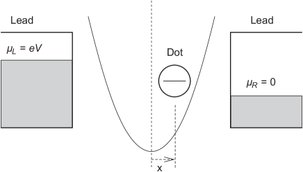
Figure 1: Model system consisting of a movable quantum dot placed between two leads. An effective elastic force acting on the dot due to its connections to the leads is described by a parabolic potential. Only one single electron state is available in the dot and the non-interacting electrons in the leads are assumed to have a constant density of states. Reprinted with permission from shuttlefedor , D. Fedorets et al., Europhys. Lett. 58, 99 (2002). $\copyright$ 2002, EDP Sciences.

At first, we consider the single-electron shuttle effect in the simplest model shuttlefedor where the grain is modeled as a single-level quantum dot (QD) that is weakly coupled (via a tunnel Hamiltonian) to the electrodes (see Fig. 1). The Hamiltonian corresponding to this model reads

$$H_{tot}=\sum_{j=L,R}H^{(j)}_{l}+H_{QD}+H_{v}+\sum_{j=L,R}H_{t}^{(j)},$$ (1)

where the Hamiltonian

$$H_{l}^{(j)}=\sum_{k}(\varepsilon_{kj}-\mu_{j})a^{{\dagger}}_{kj}a_{kj}$$ (2)

describes noninteracting electrons in the left ($j=L$) and right ($j=R$) leads, which are kept at different chemical potential $\mu_{j}$ and have a constant density states $\nu_{j}$; $a^{{\dagger}}_{kj}(a_{kj})$ creates (annihilates) an electron with momentum $k$ in lead $j$. The quantum dot is described by two parts. It is single electron level Hamiltonian and Hamiltonian of harmonic potential in which QD vibrates

$$H_{QD}=\varepsilon_{0}c^{{\dagger}}c-dxc^{{\dagger}}c,$$ (3)

$$H_{v}=\frac{1}{2}(x^{2}+p^{2}),$$ (4)

where $c^{{\dagger}}(c)$ is the creation (annihilation) operator for an electron at the dot, $\varepsilon_{0}$ is the energy of the resonant level, $x$ is the dimensionless coordinate operator (normalized by the amplitude $x_{0}$ of zero-point fluctuations, $x_{0}=\sqrt{\hbar/M\omega_{0}}$, $M$ is the mass of QD), $p$ is the corresponding momentum operator ($[x,p]=i$), $\omega_{0}$ is the frequency of vibrons, $d=eE/(M\omega_{0}^{2}x_{0})$ is characteristic electromechanical interaction constant. For convenience we use dimensionless variables. The physical meaning of the second term in Eq. (3) for usual shuttle systems is the interaction energy due to the coupling of the electron charge density on the dot with the electric field ($E$) in the gap between electrodes. Here, for convenience, all energies measure in units $\hbar\omega_{0}$, time in units of $\omega_{0}^{-1}$. Note, that in general the mechanism of electromechanical interaction could have different nature (electrostatic interaction charge on the dot with gate electrode, interaction in magnetic field due the Lorentz force, due exchange force between electrons with spin and spin polarized leads, see next Sections).

The tunneling Hamiltonian $H_{t}^{(j)}$ in Eq. (1) has the form:

$$H_{t}^{(j)}=\sum_{k}t_{0j}\exp(jx/\lambda)a_{kj}^{{\dagger}}c+h.c.$$ (5)

Here $j=\pm$ for $L/R$ electrodes, $t_{0j}$ is the bare tunneling amplitude, which corresponds to a weak dot-electrode coupling, $\lambda$ is the characteristic tunneling length. The explicit coordinate dependence in the tunneling Hamiltonian indicates sensitivity of tunnel matrix elements to a shift of the quantum dot center-of-mass coordinate with respect to its equilibrium ($x_{cm}=0$) position. The $x$-dependence in Eq. (5) represents also additional interaction with vibronic degree of freedom.

Even in such a simple formulation the single-electron shuttle problem is quite complex. In this section we review some main results of electron shuttling (without involving the spin degree of freedom) and present the basic idea of solution’s method based on the equation of motion for the matrix density. The advantage of this method is that it is possible to explicitly consider the quantum dot dynamics in quantum regime and take into account the coherent dynamics of spin electron’s states in a magnetic field, see the next section.

The time evolution of the system is obtained from the Liouville-von Neumann equation for the total density matrix

$$i\hbar\partial_{t}\hat{\sigma}(t)=[H,\hat{\sigma}(t)].$$ (6)

In order to consider the dynamics of the electronic state in the dot and the vibronic degrees of freedom we reduce the total density operator by tracing over all electronic states in the leads, $\rho(t)=\mathrm{Tr}_{leads}\{\sigma(t)\}$. We assume that electrons in the leads are in equilibrium and that they are not affected by the coupling to the dot. So, we factorize the density matrix, $\sigma(t)\approx\rho(t)\otimes\sigma_{leads}$ (this approximation is always valid for $\Gamma_{j}=2\pi\nu_{j}|t_{0j}|^{2}\exp[\mp x/\lambda]\ll 1$). After shifting the $x$-axis by $d/2$ we get the system of equation of motion for the diagonal elements of density matrix $\rho_{0}=\langle 0|\rho|0\rangle$ and $\rho_{1}=\langle 1|\rho|1\rangle$, where $|1\rangle=d^{{\dagger}}|0\rangle$, as

$$\partial_{t}\rho_{0}=-i\left[(H_{v}+\frac{d}{2}x,\rho_{0}\right]-\frac{1}{2}\{\overline{\Gamma}_{L}(x),\rho_{0}\}$$ (7)

$$+\sqrt{\overline{\Gamma}_{R}(x)}\rho_{1}\sqrt{\overline{\Gamma}_{R}(x)},$$

$$\partial_{t}\rho_{1}=-i\left[(H_{v}-\frac{d}{2}x,\rho_{1}\right]-\frac{1}{2}\{\overline{\Gamma}_{R}(x),\rho_{1}\}$$

$$+\sqrt{\overline{\Gamma}_{L}(x)}\rho_{0}\sqrt{\overline{\Gamma}_{L}(x)},$$ (8)

where $\overline{\Gamma}_{j}(x)=\Gamma_{j}(x+d/2)]$. The off-diagonal density matrix elements are decoupled from the equation of motion of the diagonal elements. It is easy to take into account dissipation of the system. The corresponding dissipation term is $L_{\gamma}\rho=-(i\gamma/2)[x,\{p,\rho\}]-(\gamma/2)[x,[x,p]]$ ($\gamma$ is the dissipation rate).

Now we find the condition under which the vibrational ground state of the oscillator becomes unstable. For this we consider the time evolution of the expectation value of the coordinate, $\bar{x}(t)=\textbf{Tr}\{x\rho_{+}\}$, and the momentum operators, $\bar{p}(t)=\textbf{Tr}\{p\rho_{+}\}$, of the island (here $\rho_{+}\equiv\rho_{0}+\rho_{1}$). To first order in $\lambda^{-1}$, for symmetric tunneling couplings $\widetilde{\Gamma}_{L}(0)=\widetilde{\Gamma}_{R}(0)=\Gamma/2$ and in the high bias voltage limit ($\mu_{L}-\mu_{R}=eV\rightarrow\infty$) the equations of motion for the first vibrational moments become closed, so that quanshuttle

$$\dot{\bar{x}}=\bar{p}, \dot{\bar{p}}=-\gamma\bar{p}-\bar{x}-\frac{d}{2}n_{-},$$

$$\dot{n}_{-}=-\Gamma n_{-}+\frac{2\Gamma}{\lambda}\bar{x},$$

where $n_{-}=1-2\bf{Tr}\rho_{1}$. The solution of Eq. (II.1) for the quantum dot displacement is $\bar{x}(t)\approx Ae^{rt}\cos(t)$, where $r=1/2(\gamma_{thr}-\gamma)$ is the rate of increment of the shuttle instability. If the dissipation rate $\gamma$ is below the threshold value $\gamma_{thr}=\Gamma d/[\lambda(\Gamma^{2})+1]$, then the expectation value of the dot coordinate grows exponentially in time and the vibrational ground state is unstable. It was shown quanshuttle that this exponential increase of the displacement drives the system into the nonlinear regime of the vibration dynamics, where the system reaches a stable steady state of developed shuttle motion.

In order to analyze this stable state (i.e. the solution of the system Eq. (7,II.1) it is convenient to use the Wigner function representation novotny , quanshuttle . The Wigner distribution function for the density operator $\rho_{+}$ is defined as

$$W_{+}(x,p)\equiv\frac{1}{2\pi}\int_{-\infty}^{+\infty}d\xi e^{-ip\xi}\left\langle x+\xi/2|\rho_{+}|x-\xi/2\right\rangle.$$ (10)

The dynamics of the oscillating QD is characterized by its trajectory (distribution) in the phase space ($x,p$) for $p^{2}/2+x^{2}/2=const$. Now we proceed to polar coordinates $(A,\varphi)$, where $x=A\sin\varphi$ and $p=A\cos\varphi$. An equation for $W_{+}(A,\varphi)$ is derived from Eqs. (7) and (II.1) after straightforward calculations (for details see quanshuttle ). To leading order in the small parameters $d/\lambda$, $\lambda^{-2}$, and $\gamma$ this equation takes the form of a stationary Fokker-Planck equation for the zeroth Fourier component of the Wigner function $\overline{W}_{+}(A)$

$$\frac{\partial}{\partial A}\left(\overline{D}_{0}(A)\frac{\partial}{\partial A}-\overline{D}_{1}(A)\right)\overline{W}_{+}(A)=0,$$ (11)

where $\overline{D}_{1}=A^{2}D_{1}(A),\overline{D}_{0}=AD_{0}(A)$ are drift- and diffusion coefficients (analytical expression of this coefficients will be presented in section for the magnetic shuttle). The normalized solution of Eq. (11) has the form of a Boltzman distribution,

$$\overline{W}_{+}=Z^{-1}\exp\left(\int_{0}^{A}dA\frac{\overline{D}_{1}(A)}{\overline{D}_{0}(A)}\right)$$ (12)

The stationary solution of the oscillating dot is localized in the phase space around points where $\overline{W}_{+}$ is maximal. From Eq. (12) one can see that the maximum of the Wigner function is determined by zeros of the drift coefficient $\overline{D}_{1}(A_{m})=0$ ($\overline{D}^{\prime}_{1}(A_{m})<0$). In the vicinity of this point, $\overline{W}_{+}$ can be approximated by a Gaussian distribution function. For the spinless shuttle problem it can be shown that $\overline{W}_{+}$ always has an extremum at $A=0$: maximum for $\gamma>\gamma_{thr}$ and minimum for $\gamma<\gamma_{thr}$. So the vibrational ground state is unstable when the dissipation is below threshold value as has been shown by solving the equation system (II.1). The function $\overline{W}_{+}$ has also a maximum for the non-zero amplitude $A_{C}$, which corresponds to the stable limit cycle amplitude of shuttle oscillations (for more details see quanshuttle ).

One can distinguish two regimes of "quantum" (for $d/\lambda\ll\lambda^{-4}$) and "quasiclassical" ($d/\lambda\gg\lambda^{-4}$) shuttle motion. In the quasiclassical regime Gaussian distribution is narrow and in quantum regime the width of distribution “bell” is of the order of $\lambda\gg 1$, i.e. the Wigner function is smeared around classical phase trajectory. It is interesting to note that a region of parameters exists where both vibrational and shuttling regimes are present (a region where the Wigner function has two maxima).

III Electro - and Spintro - Mechanics of Magnetic shuttle devices

In this Section we will explore new functionalities that emerge when nanomechanical devices are partly or completely made of magnetic materials. The possibility of magnetic ordering brings new degrees of freedom into play in addition to the electronic and mechanical ones considered so far, opening up an exciting perspective towards utilising magneto-electro-mechanical transduction for a large variety of applications. Device dimensions in the nanometer range mean that a number of mesoscopic phenomena in the electronic, magnetic and mechanical subsystems can be used for quantum coherent manipulations. In comparison with the electromechanics of the nanodevices considered above the prominent role of the electronic spin in addition to the electric charge should be taken into account.

The ability to manipulate and control spins via electrical 9 ; 10 ; 11 magnetic 12 and optical kadigrobov ; 13 means has generated numerous applications in metrology 14 in recent years. A promising alternative method for spin manipulation employs a mechanical resonator coupled to the magnetic dipole moment of the spin(s), a method which could enable scalable quantum information architectures 15 and sensitive nanoscale magnetometry 16 ; 17 ; 18 . Magnetic resonance force microscopy (MRFM) was suggested as a means to improve spin detection to the level of a single spin and thus enable three dimensional imaging of macromolecules with atomic resolution. In this technique a single spin, driven by a resonant microwave magnetic field interacts with a ferromagnetic particle. If the ferromagnetic particle is attached to a cantilever tip, the spin changes the cantilever vibration parameters 21 . The possibility to detect 21 and monitor the coherent dynamics of a single spin mechanically 22 has been demonstrated experimentally. Several theoretical suggestions concerning the possibility to test single-spin dynamics through an electronic transport measurement were made recently 24 ; 25 ; 26 ; 27 . Complementary studies of the mechanics of a resonator coupled to spin degrees of freedom by detecting the spin dynamics and relaxation were suggested in 24 ; 25 ; 26 ; 27 ; 28 ; 29 ; 30 ; 31 and carried out in 32 . Electronic spin-orbit interaction in suspended nanowires was shown to be an efficient tool for detection and cooling of bending-mode nanovibrations as well as for manipulation of spin qubit and mechanical quantum vibrations 33 ; 34 ; 35 .

An obvious modification of the nano-electro-mechanics of magnetic shuttle devices originates from the spin-splitting of electronic energy levels, which results in the known phenomenon of spin-dependent tunneling. Spin-controlled nano-electro-mechanics which originates from spin-controlled transport of electric charge in magnetic NEM systems is represented by number of new magneto-electro-mechanical phenomena.

Qualitatively new opportunities appear when magnetic nanomechanical devices are used. They have to do with the effect of the short-ranged magnetic exchange interaction between the spin of electrons and magnetic parts of the device. In this case the spin of the electron rather than its electrical charge can be the main source of the mechanical force acting on movable parts of the device. This leads to new physics compared with the usual electromechanics of non-magnetic devices, for which we use the term spintro-mechanics. In particular it becomes possible for a movable central island to shuttle magnetization between two magnetic leads even without any charge transport between the leads. The result of such a mechanical transportation of magnetization is a magnetic coupling between nanomagnets with a strength and sign that are mechanically tunable.

In this Section we will review some early results that involve the phenomena mentioned above. These only amount to a first step in the exploration of new opportunities caused by the interrelation between charge, spin and mechanics on a nanometer length scale.

III.1 Spin-controlled shuttling of electric charge

By manipulating the interaction between the spin of electrons and external magnetic fields and/or the internal interaction in magnetic materials, spin-controlled nanoelectromechanics may be achieved.

A new functional principle — spin-dependent shuttling of electrons — for low magnetic field sensing purposes was proposed by Gorelik et al. in Ref. r88, . This principle may lead to a giant magnetoresistance effect in external magnetic fields as low as 1-10 Oe in a magnetic shuttle device if magnets with highly spin-polarized electrons (half metals r83 ; r84 ; r85 ; r86 ; r87 ) are used as leads in a magnetic shuttle device. The key idea is to use the external magnetic field to manipulate the spin of shuttled electrons rather than the magnetization of the leads. Since the electron spends a relatively long time on the shuttle, where it is decoupled from the magnetic environment, even a weak magnetic can rotate its spin by a significant angle. Such a rotation allows the spin of an electron that has been loaded onto the shuttle from a spin-polarized source electrode to be reoriented in order to allow the electron finally to tunnel from the shuttle to the (differently) spin-polarized drain lead. In this way the shuttle serves as a very sensitive “magnetoresistor" device. The model employed in Ref. r88, assumes that the source and drain are fully polarized in opposite directions. A mechanically movable quantum dot (described by a time-dependent displacement $x(t)$), where a single energy level is available for electrons, performs driven harmonic oscillations between the leads. The external magnetic field, $H$, is perpendicular to the orientations of the magnetization in both leads and to the direction of the mechanical motion.

The spin-dependent part of the Hamiltonian is specified as

$$H_{\rm magn}(t)=J(t)(a^{{\dagger}}_{\uparrow}a_{\uparrow}-a^{{\dagger}}_{\downarrow}a_{\downarrow})-\frac{g\mu H}{2}(a^{{\dagger}}_{\uparrow}a_{\downarrow}+a^{{\dagger}}_{\downarrow}a_{\uparrow}),$$ (13)

where $J(t)=J_{R}(t)-J_{L}(t)$, $J_{L(R)}(t)$ are the molecular fields induced by exchange interactions between the on-grain electron and the left(right) lead, $g$ is the gyromagnetic ratio and $\mu$ is the Bohr magneton. The proper Liouville-von Neumann equation for the density matrix is analyzed and an average electrical current is calculated for the case of large bias voltage.

In the limit of weak exchange field, $J_{max}\ll\mu H$ one may neglect the influence of the magnetic leads on the on-dot electron spin dynamics. The resulting current is

$$I=\frac{e\omega_{0}}{\pi}\frac{\sin^{2}(\vartheta/2)\tanh(w/4)}{\sin^{2}(\vartheta/2)+\tanh^{2}(w/4)}$$ (14)

where $w$ is the total tunneling probability during the contact time $t_{0}$, while $\vartheta\sim\pi g\mu H/\hbar\omega_{0}$ is the rotation angle of the spin during the “free-motion" time.

The theory r88 predicts oscillations in the magnetoresistance of the magnetic shuttle device with a period $\Delta H_{p}$, which is determined from the equation $\hbar\omega_{0}=g\mu(1+w)\Delta H_{p}$. The physical meaning of this relation is simple: every time when $\omega_{0}/\Omega=n+1/2$ ($\Omega=g\mu H/\hbar$ is the spin precession frequency in a magnetic field) the shuttled electron is able to flip fully its spin to remove the “spin-blockade" of tunneling between spin polarized leads having their magnetization in opposite directions. This effect can be used for measuring the mechanical frequency thus providing dc spectroscopy of nanomechanical vibrations.

Spin-dependent shuttling of electrons as discussed above is a property of non-interacting electrons, in the sense that tunneling of different electrons into (and out of) the dot are independent events. The Coulomb blockade phenomenon adds a strong correlation of tunneling events, preventing fluctuations in the occupation of electronic states on the dot. This effect crucially changes the physics of spin-dependent tunneling in a magnetic NEM device. One of the remarkable consequences is the Coulomb promotion of spin-dependent tunneling predicted in Ref. 1, . In this work a strong voltage dependence of the spin-flip relaxation rate on a quantum dot was demonstrated. Such relaxation, being very sensitive to the occupation of spin-up and spin-down states on the dot, can be controlled by the Coulomb blockade phenomenon. It was shown in Ref. 1, that by lifting the Coulomb blockade one stimulates occupation of both spin-up and spin-down states thus suppressing spin-flip relaxation on the dot. In magnetic devices with highly spin-polarized electrons electronic spin-flip can be the only mechanism providing charge transport between oppositely magnetized leads. In this case the onset of Coulomb blockade, by increasing the spin-flip relaxation rate, stimulates charge transport through a magnetic SET device (Coulomb promotion of spin-dependent tunneling). Spin-flip relaxation also modifies qualitatively the noise characteristics of spin-dependent single-electron transport. In Refs. 2, ; 3, it was shown that the low-frequency shot noise in such structures diverges as the spin relaxation rate goes to zero. This effect provides an efficient tool for spectroscopy of extremely slow spin-flip relaxation in quantum dots. Mechanical transportation of a spin-polarized dot in a magnetic shuttle device provides new opportunities for studying spin-flip relaxation in quantum dots. The reason can be traced to a spin-blockade of the mechanically aided shuttle current that occurs in devices with highly polarized and colinearly magnetized leads. As was shown in Ref. 4, the above effect results in giant peaks in the shot-noise spectral function, wherein the peak heights are only limited by the rates of electronic spin flips. This enables a nanomechanical spectroscopy of rare spin-flip events, allowing spin-flip relaxation times as long as $10~{}\mu$s to be detected.

The spin-dependence of electronic tunneling in magnetic NEM devices permits an external magnetic field to be used for manipulating not only electric transport but also the mechanical performance of the device. This was demonstrated in Refs. s90, ; 5, . A theory of the quantum coherent dynamics of mechanical vibrations, electron charge and spin was formulated and the possibility to trigger a shuttle instability by a relatively weak magnetic field was demonstrated. It was shown that the strength of the magnetic field required to control nanomechanical vibrations decreases with an increasing tunnel resistance of the device and can be as low as 10 Oe for giga-ohm tunnel structures.

A new type of nanoelectromechanical self excitation caused entirely by the spin splitting of electronic energy levels in an external magnetic field was predicted in Ref. 6, for a suspended nanowire, where mechanical motion in a magnetic field induces an electromotive coupling between electronic and vibrational degrees of freedom. It was shown that a strong correlation between the occupancy of the spin-split electronic energy levels in the nanowire and the velocity of flexural nanowire vibrations provides energy supply from the source of DC current, flowing through the wire, to the mechanical vibrations thus making possible stable, self-supporting bending vibrations. Estimations made in Ref. 6, show that in a realistic case the vibration amplitude of a suspended carbon nanotube (CNT) of the order of 10 nm can be achieved if magnetic field of 10 T is applied.

III.2 Spintro-mechanics of magnetic shuttle devices

New phenomena, qualitatively different from the electromechanics of nonmagnetic shuttle systems, may appear in magnetic shuttle devices in a situation when short-range magnetic exchange forces become comparable in strength to the long-range electrostatic forces between the charged elements of the device 6 . There is convincing evidence that the exchange field can be several tesla at a distance of a few nanometers from the surface of a ferromagnet radic4 ; radic5 ; radic6 ; radic9 . Because of the exponential decay of the field this means that the force experienced by a single-electron spin in the vicinity of magnetic electrodes can be very large. These spin-dependent exchange forces can lead to various “spintro-mechanical" phenomena.

Mechanical effects produced by a long-range electrostatic force and short-ranged exchange forces on a movable quantum dot are illustrated in Fig. 2.

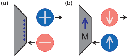
Figure 2: A movable quantum dot in a magnetic shuttle device can be displaced in response to two types of force: (a) a long-range electrostatic force causing an electromechanical response if the dot has a net charge, and (b) a short-range magnetic exchange force leading to “spintromechanical" response if the dot has a net magnetization (spin). The direction of the force and displacements depends on the relative signs of the charge and magnetization, respectively. Reprinted with permission from 7 , R. I. Shekhter et al., Phys. Rev. B 86, 100404 (2012). $\copyright$ 2012, American Physical Society.

The electrostatic force acting on the dot, placed in the vicinity of a charged electrode (Fig. 2(a)), is determined by the electric charge accumulated on the dot. In contrast, the exchange force induced by a neighboring magnet depends on the net spin accumulated on the dot. While the electrostatic force changes its direction if the electric charge on the dot changes its sign, the spin-dependent exchange force is insensitive to the electric charge but it changes direction if the electronic spin projection changes its sign. A very important difference between the two forces is that the electrostatic force changes only as a result of injection of additional electrons into (out of) the dot while the spintronic force can be changed due to the electron spin dynamics even for a fixed number of electrons on the dot (as is the case if the dot and the leads are insulators). In this case interesting opportunities arise from the possibility of transducing the dynamical variations of electronic spin (induced, e.g., by magnetic or microwave fields) to mechanical displacements in the NEM device. In Ref. 7, a particular spintromechanical effect was discussed – a giant spin-filtering of the electron current (flowing through the device) induced by the formation of what we shall call a “spin-polaronic state".

The Hamiltonian that describes the magnetic nanomechanical SET device in Ref. 7, has the standard form (its spin-dependent part depends now on the mechanical displacement of the dot). Hence $H=H_{lead}+H_{tunnel}+H_{dot}$, where $H_{leads}=\sum_{k,\sigma,s}\varepsilon_{ks\sigma}a^{{\dagger}}_{ks\sigma}a_{ks\sigma}$ describes electrons (labeled by wave vector $k$ and spin $\sigma=\uparrow,\downarrow$) in the two leads ($s=L,R$). Electron tunneling between the leads and the dot is modeled as

$$H_{tunnel}=\sum_{k,\sigma,s}T_{s}(x)a^{{\dagger}}_{ks\sigma}c_{\sigma}+H.c.$$ (15)

where the matrix elements $T_{s}(x)=T^{(0)}_{s}\exp(\mp x/\lambda)$ ($\lambda$ is the characteristic tunneling length) depend on the dot position $x$. The Hamiltonian of the movable single-level dot is

$$H_{dot}=\hbar\omega_{0}b^{{\dagger}}b+\sum_{\sigma}n_{\sigma}[\varepsilon_{0}-{\rm sgn}(\sigma)J(x)]+U_{C}n_{\uparrow}n_{\downarrow},$$ (16)

where ${\rm sgn}(\uparrow,\downarrow)=\pm 1$, $U_{C}$ is the Coulomb energy associated with double occupancy of the dot and the eigenvalues of the electron number operators $n_{\sigma}$ is $0$ or $1$. The position dependent magnitude $J(x)$ of the spin dependent shift of the electronic energy level on the dot is due to the exchange interaction with the magnetic leads. Here we expand $J(x)$ to linear order in $x$ so that $J(x)=J^{(0)}+jx$ and without loss of generality assume that $J^{(0)}=0$.

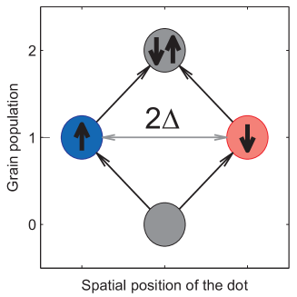
Figure 3: Diagram showing how the equilibrium position of the movable dot depends on its net charge and spin. The difference in spatial displacements discriminates transport through a singly occupied dot with respect to the electron spin. Reprinted with permission from 7 , R. I. Shekhter et al., Phys. Rev. B 86, 100404 (2012). $\copyright$ 2012, American Physical Society.

The modification of the exchange force, caused by changing the spin accumulated on the dot, shifts the equilibrium position of the dot with respect to the magnetic leads of the device. Since the electron tunneling matrix element is exponentially sensitive to the position of the dot with respect to the source and drain electrodes one expects a strong spin-dependent renormalization of the tunneling probability, which exponentially discriminates between the contributions to the total electrical current from electrons with different spins. This spatial separation of dots with opposite spins is illustrated in Fig. 3. While changing the population of spin-up and spin-down levels on the dot (by changing e.g. the bias voltage applied to the device) one shifts the spatial position $x$ of the dot with respect to the source/drain leads. It is important that the Coulomb blockade phenomenon prevents simultaneous population of both spin states. If the Coulomb blockade is lifted the two spin states become equally populated with a zero net spin on the dot, $\textbf{S}=0$. This removes the spin-polaronic deformation and the dot is situated at the same place as a non-populated one. In calculations a strong modification of the vibrational states of the dot, which has to do with a shift of its equilibrium position, should be taken into account. This results in a so-called Franck-Condon blockade of electronic tunneling 116 ; ratner . The spintro-mechanical stimulation of a spin-polarized current and the spin-polaronic Franck-Condon blockade of electronic tunneling are in competition and their interplay determines a non-monotonic voltage dependence of the giant spin-filtering effect.

To understand the above effects in more detail consider the analytical results of Ref. 7, . A solution of the problem can be obtained by the standard sequential tunneling approximation and by solving a Liouville equation for the density matrix for both the electronic and vibronic subsystems. The spin-up and spin-down currents can be expressed in terms of transition rates (energy broadening of the level) and the occupation probabilities for the dot electronic states. For simplicity we consider the case of a strongly asymmetric tunneling device. At low bias voltage and low temperature the partial spin current is

$$I_{\sigma}\sim\frac{e\Gamma_{L}}{\hbar}\exp\left(\frac{1}{2}\left[\frac{x_{0}^{2}}{\lambda^{2}}-\left(\frac{x_{0}}{\hbar\omega_{0}}\right)^{2}\right]-{\rm sgn}(\sigma)\beta\right),$$ (17)

where $\beta=x_{0}^{2}/\hbar\omega_{0}\lambda$. In the high bias voltage (or temperature) regime, $max\{eV,T\gg E_{p}\}$, where the polaronic blockade is lifted (but double occupancy of the dot is still prevented by the Coulomb blockade), the current expression takes the form

$$I_{\sigma}\sim\frac{e\Gamma_{L}}{\hbar}\exp\left(\left[2n_{B}+1\right]\frac{x_{0}^{2}}{\lambda^{2}}-2\,{\rm sgn}(\sigma)\beta\right),$$ (18)

where $n_{B}$ is Bose-Einstein distribution function. The scale of the polaronic spin-filtering of the device is determined by the ratio $\beta$ of the polaronic shift of the equilibrium spatial position of a spin-polarized dot and the electronic tunneling length. For typical values of the exchange interaction and mechanical properties of suspended carbon nanotubes this parameter is about 1-10. As was shown this is enough for the spin filtering of the electrical current through the device to be nearly 100 % efficient. The temperature and voltage dependence of the spin-filtering effect is presented in Fig. 4. The spin filtering effect and the Franck-Condon blockade

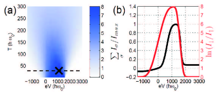
Figure 4: Spin polarization of the current through the model NEM-SET device under discussion. Reprinted with permission from 7 , R. I. Shekhter et al., Phys. Rev. B 86, 100404 (2012). $\copyright$ 2012, American Physical Society.

both occur at low voltages and temperatures (on the scale of the polaronic energy; see Fig. 4 (a)). An increase of the voltage applied to the device lifts the Franck-Condon blockade, which results in an exponential increase of both the current and the spin-filtering efficiency of the device. This increase is blocked abruptly at voltages for which the Coulomb blockade is lifted. At this point a double occupation of the dot results in spin cancellation and removal of the spin-polaronic segregation. This leads to an exponential drop of both the total current and the spin polarization of the tunnel current (Fig. 4 (b)). As one can see in Fig. 4 prominent spin filtering can be achieved for realistic device parameters. The temperature of operation of the spin-filtering device is restricted from above by the Coulomb blockade energy. One may, however, consider using functionalized nanotubes pulkin20 or graphene ribbons pulkin21 with one or more nanometer-sized metal or semiconductor nanocrystal attached. This may provide a Coulomb blockade energy up to a few hundred kelvin, making spin filtering a high temperature effect 7 .

III.3 Spintronics of shuttles

In this subsection we discuss the possibility to manipulate the spin of tunneling electrons by an external magnetic field and how it can affect electron transport through a nanoelectromechanical device. In the simplest model, we assume that the left and right electrodes are fully spin polarized. The movable single level quantum dot (in the absence of a magnetic field) can vibrate in the gap between two leads. A bias voltage is applied but electron transport through the system is blocked since the source and drain leads are fully spin polarized in opposite direction. An external magnetic field applied pendicular to the direction of the magnetization in the electrode leads to precession of the electron spin of the quantum dot and as a consequence the electron transport is unblocked. The Hamiltonian of the system has the form 5 of Eq. (1) with $H_{leads}=\Sigma_{jk}\varepsilon_{j}(k)c^{{\dagger}}_{jk}c_{jk}$ ($j=L,R\rightarrow j=(\uparrow,\downarrow)$) and

$$H_{QD}=(\varepsilon_{0}-dx)\sum_{\sigma}c^{{\dagger}}_{\sigma}c_{\sigma}-\frac{h}{2}(c^{{\dagger}}_{\uparrow}c_{\downarrow}+c^{{\dagger}}_{\downarrow}c_{\uparrow})+Uc^{{\dagger}}_{\uparrow}c_{\uparrow}c^{{\dagger}}_{\downarrow}c_{\downarrow},$$ (19)

where $h=g\mu_{B}H/\hbar\omega_{0}$ is the dimensionless magnetic field. To analyze this system we use the method described in Section 2. A quantum master equation for the reduced density matrix operator $\rho_{0}\equiv\langle 0\mid\rho\mid 0\rangle$, $\rho_{\uparrow}\equiv\langle\uparrow\mid\rho\mid\uparrow\rangle$, $\rho_{\downarrow}\equiv\langle\downarrow\mid\rho\mid\downarrow\rangle$, and $\rho_{\uparrow\downarrow}\equiv\langle\uparrow\mid\rho\mid\downarrow\rangle$ is obtained in analogy with the spinless case

$$\frac{\partial\rho_{0}}{\partial t}=-i\left[{H}_{v}+xd,\rho_{0}\right]$$

$$\hskip 31.2982pt-\left\{\overline{\Gamma}_{L}(x),\rho_{0}\right\}/2+\sqrt{\overline{\Gamma}_{R}(x)}\rho_{\downarrow}\sqrt{\overline{\Gamma}_{R}(x)},$$ (20)

$$\frac{\partial\rho_{\downarrow}}{\partial t}=-i\left[{H}_{v},\rho_{\downarrow}\right]$$

$$\hskip 31.2982pt+i\frac{h}{2}\left(\rho_{\uparrow\downarrow}-\rho_{\uparrow\downarrow}\right)-\frac{1}{2}\left\{{\overline{\Gamma}_{+}(x)},\rho_{\downarrow}\right\},$$ (21)

$$\frac{\partial\rho_{\uparrow}}{\partial t}=-i\left[{H}_{v},\rho_{\uparrow}\right]-i\frac{h}{2}\left(\rho_{\uparrow\downarrow}-\rho_{\uparrow\downarrow}\right)$$

$$\hskip 31.2982pt+\sqrt{\overline{\Gamma}_{L}(x)}\rho_{0}\sqrt{\overline{\Gamma}_{L}(x)}+\sqrt{\overline{\Gamma}_{R}(x)}\rho_{2}\sqrt{\overline{\Gamma}_{R}(x)},$$ (22)

$$\frac{\partial\rho_{\uparrow\downarrow}}{\partial t}=-i\left[{H}_{v},\rho_{\uparrow\downarrow}\right]+i\frac{h}{2}[\rho_{\downarrow}-\rho_{\uparrow}]-\frac{1}{2}\rho_{\uparrow\downarrow}\overline{\Gamma}_{+}(x),$$ (23)

$$\frac{\partial\rho_{\downarrow\uparrow}}{\partial t}=-i\left[{H}_{v},\rho_{\downarrow\uparrow}\right]-i\frac{h}{2}[\rho_{\downarrow}-\rho_{\uparrow}]-\frac{1}{2}\overline{\Gamma}_{+}(x)\rho_{\uparrow\downarrow},$$ (24)

$$\frac{\partial\rho_{2}}{\partial t}=-i\left[{H}_{v}-xd,\rho_{2}\right]$$

$$\hskip 31.2982pt-\left\{\overline{\Gamma}_{R}(x),\rho_{2}\right\}/2+\sqrt{\overline{\Gamma}_{L}(x)}\rho_{\uparrow}\sqrt{\overline{\Gamma}_{L}(x)},$$ (25)

where $\overline{\Gamma}_{+}(x)=\overline{\Gamma}_{L}(x)+\overline{\Gamma}_{R}(x)$. The set of equations (III.3)-(III.3) is derived in the high bias voltage limit: $eV/2-\varepsilon_{0}-U\gg\hbar\omega_{0}$. In general, the problem can be solved in two limits with and without the Coulomb blockade regime. In the Coulomb blockade regime the second electron can not tunnel onto the quantum dot due to Coulomb repulsion. Hence the probability for double occupancy $\rho_{2}\rightarrow 0$. First, we focus on the case without Coulomb blockade.

Here we repeat the analysis scheme for the evolution of the stationary solution $\overline{W}_{+}(A)$ for the probability of the shuttle to vibrate with an amplitude $A$. Expanding the function $\overline{D}_{1}(A)$ around $A=0$ one can get the condition for the shuttle instability $\gamma<\gamma_{thr}=\Gamma(2h^{2}d)/\lambda(h^{2}+\Gamma^{2})$. As in the case of spinless electron, the function $W_{+}$ has a maximum at $A=0$ (stable point) when dissipation rate $\gamma$ is above the threshold value. In the opposite case the vibrational ground state is unstable.

The positive bounded function $\beta_{0}(A,h)=(2\overline{D}_{1}(A)-\gamma)\lambda/d$ has only one maximum and monotonically decreases for large $A$. In 5 it was shown that if $h<\sqrt{3}\Gamma$, the function $\beta_{0}$ has a maximum at $A=0$, while for $h>\sqrt{3}\Gamma$, this function has a minimum at $A=0$. The structure of the function $\beta_{0}$ determines the behavior of the system in the parameter space $d-h$ (or $\gamma-h$). There are several areas or phases. In the first phase (vibronic), defined by $d/\gamma\lambda<1/h[max\beta_{0}(A)]$, the system is in the lowest vibrational state ($A=0$ is a stable point). The shuttle phase is developed when $\gamma<\gamma_{thr}$ and there is only one stable point at $A\neq 0$. The third phase is the mixed phase. It appears because the two above phases become unstable if $h$ exceeds the critical value $\sqrt{3}\Gamma$.

In the Coulomb blockade regime the same analysis gives that $\overline{D}_{1}(A)$ is positive for all values of $h$ if $\Gamma<4/3$. On the other hand, if $\Gamma>4/3$, there is a range of magnetic field strenghts where a shuttle instability does not occur. In particular, when $\Gamma\gg 1$ this interval is $0<h<\Gamma/\sqrt{2}$. This implies that in the adiabatic regime of charge transport ($\Gamma\gg 1$) in weak magnetic field there is no instability and the electrically driven electron shuttle is realized only in strong magnetic fields.

III.4 Electron Shuttle Based on Electron Spin

In the previous subsection we studied the shuttle instability in the case of an electromechanical coupling between the quantum dot and the leads. In the Coulomb blockade regime a shuttle instability appears if an external magnetic field $h$ exceeds the critical value $h_{\text{cr}}=\sqrt{3}\Gamma$. Here we will study the shuttle instability in the case when the interaction between the dot and the leads is due to a magnetic (exchange) coupling kulinichprl .

The Hamiltonian of the system is similar to the one considered in Section III. C. The only difference is that the quantum dot Hamiltonian reads

$${H}_{dot}=\varepsilon_{0}(a^{\dagger}_{\uparrow}a_{\uparrow}+a^{\dagger}_{\downarrow}a_{\downarrow})$$

$$\hskip 25.6073pt-J_{L}(x)(a^{\dagger}_{\uparrow}a_{\uparrow}-a^{\dagger}_{\downarrow}a_{\downarrow})-J_{R}(x)(a^{\dagger}_{\downarrow}a_{\downarrow}-a^{\dagger}_{\uparrow}a_{\uparrow})$$

$$\hskip 25.6073pt-\frac{g\mu H}{2}(a^{\dagger}_{\uparrow}a_{\downarrow}+a^{\dagger}_{\downarrow}a_{\uparrow})-Ua^{\dagger}_{\uparrow}a^{\dagger}_{\downarrow}a_{\uparrow}a_{\downarrow}\,.$$ (26)

In what follows we will consider the symmetrical case, $J_{R}(x)=J_{L}(-x)$ and restrict ourselves to the Coulomb blockade regime, $U\sim e^{2}/2C>\mid eV/2-\varepsilon_{0}\mid$.

Following Ref.5 one gets equations of motion for the reduced density matrix operators $\rho_{0}\equiv\langle 0\mid\rho\mid 0\rangle$, $\rho_{\uparrow}\equiv\langle\uparrow\mid\rho\mid\uparrow\rangle$, $\rho_{\downarrow}\equiv\langle\downarrow\mid\rho\mid\downarrow\rangle$, and $\rho_{\uparrow\downarrow}\equiv\langle\uparrow\mid\rho\mid\downarrow\rangle$:

$$\frac{\partial\rho_{0}}{\partial t}=-i\left[{H}_{v},\rho_{0}\right]$$

$$\hskip 31.2982pt-\left\{\Gamma_{L}(x),\rho_{0}\right\}/2+\sqrt{\Gamma_{R}(x)}\rho_{\downarrow}\sqrt{\Gamma_{R}(x)},$$ (27)

$$\frac{\partial\rho_{\uparrow}}{\partial t}=-i\left[{H}_{v},\rho_{\uparrow}\right]+i\left[J(x),\rho_{\uparrow}\right]$$

$$\hskip 31.2982pt-ih\left(\rho_{\uparrow\downarrow}-\rho^{{\dagger}}_{\uparrow\downarrow}\right)/2+\sqrt{\Gamma_{L}(x)}\rho_{0}\sqrt{\Gamma_{L}(x)},$$ (28)

$$\frac{\partial\rho_{\downarrow}}{\partial t}=-i\left[{H}_{v},\rho_{\downarrow}\right]-i\left[J(x),\rho_{\downarrow}\right]$$

$$\hskip 31.2982pt+ih\left(\rho_{\uparrow\downarrow}-\rho^{{\dagger}}_{\uparrow\downarrow}\right)/2-\left\{\Gamma_{R}(x),\rho_{\downarrow}\right\}/2,$$ (29)

$$\frac{\partial\rho_{\uparrow\downarrow}}{\partial t}=-i\left[{H}_{v},\rho_{\uparrow\downarrow}\right]+i\left\{J(x),\rho_{\uparrow\downarrow}\right\}$$

$$\hskip 36.98866pt+ih\left(\rho_{\downarrow}-\rho_{\uparrow}\right)/2-\rho_{\uparrow\downarrow}\Gamma_{R}(x)/2$$ (30)

In Eqs. (III.4)-(30) $\,\Gamma_{j}(x)=\Gamma\text{exp}(j2x/\lambda)$ and $J(x)=J_{L}(x)-J_{R}(x)$. In what follows we assume a linear $x$-dependence of $J(x)$: $J(x)\simeq-\alpha x+...,\,\alpha=2J^{\prime}_{R}(0)>0$.

The difference between our operator equations and the corresponding equations in Ref. 5 (rewritten for the Coulomb blockade case) is the appearance of terms induced by the coordinate-dependent exchange interaction $J(x)$. These appear in Eqs. (III.4)-(30) as a commutator term for $\rho_{\uparrow}$ and $\rho_{\downarrow}$ and as an anti-commutator term for $\rho_{\uparrow\downarrow}$. In contrast to the electrically driven shuttle, the driving force in our case is strongly connected to the spin dynamics, which results in a completely different dependence of the shuttle behavior on magnetic field.

Both linear and nonlinear regimes of the shuttling dynamics can be conveniently analyzed by using the Wigner function representation of the density operators novotny . This approach allows one to calculate the Wigner distribution function $W_{\rho}(x,p)$ for the vibrational degree of freedom to lowest order in the small parameters $\alpha$ and $1/\lambda$ for small (compared to $\lambda$) shuttle vibration amplitudes $A$. The relevant Wigner function, $W_{\Sigma}^{(0)}(A)$, averaged over the shuttle phase $\varphi$ ($x=A\sin\varphi$), solves the stationary Fokker-Planck equation as in Eq. (11) with drift- and diffusion coefficients containing the factors

$$D_{1}=\frac{\alpha}{\lambda}\frac{h^{2}\Gamma^{3}}{\Gamma^{2}+3h^{2}}\frac{3\Gamma^{2}+3-h^{2}}{Q_{0}(\Gamma,h)}$$ (31)

$$D_{0}=\frac{h^{2}\Gamma}{\Gamma^{2}+3h^{2}}\left[\frac{\alpha^{2}Q_{1}(\Gamma,h)+\lambda^{-2}Q_{0}(\Gamma,h)}{2Q_{0}(\Gamma,h)}\right]$$ (32)

respectively, where

$$Q_{0}(\Gamma,h)=\left(1-h^{2}-2\Gamma^{2}\right)^{2}+\frac{\Gamma^{2}}{4}\left(\Gamma^{2}+3h^{2}-5\right)^{2},\hskip 8.5359pt$$ (33)

$$Q_{1}(\Gamma,h)=\left(1+\frac{9\Gamma^{2}}{4}\right)\left(1+h^{2}+2\Gamma^{2}\right)-\frac{5\Gamma^{4}}{4}.\hskip 28.45274pt$$ (34)

In Eqs. (31)-(34) all energies are normalized with respect to the energy quantum $\hbar\omega$ of the mechanical vibrations: $\hbar\omega\rightarrow 1$, $g\mu H/\hbar\omega\rightarrow h$, $J(x)/\hbar\omega\rightarrow J(x)$, $\Gamma_{j}(x)/\omega\rightarrow\Gamma_{j}(x)$ [$\hbar\Gamma_{j}(x)=2\pi\nu\mid T_{j}(x)\mid^{2}$ are partial level widths].

For $A\ll 1$ the solution of Eq. (11) takes the form of a Boltzmann distribution function, $W_{\Sigma}^{(0)}\sim\exp(-\beta{\cal E})$, where ${\cal E}=A^{2}/2$ is the dot’s vibrational energy and $1/\beta$, where

$$\beta=\left(\frac{2\alpha\Gamma^{2}}{\lambda}\right)\frac{h^{2}-3\Gamma^{2}-3}{\alpha^{2}Q_{1}(\Gamma,h)+\lambda^{-2}Q_{0}(\Gamma,h)}\,,$$ (35)

is an effective temperature. Since the functions $Q_{0}$ and $Q_{1}$ are positive, the sign of the effective temperature is determined by the relation between magnetic field, level width and vibration quantum. In particular the effective temperature is negative at small magnetic fields, $|H|<H_{c}$, where (reverting to dimensional variables) $g\mu H_{c}=\hbar\sqrt{3\left(\Gamma^{2}+\omega^{2}\right)}$.

A negative $\beta$ implies that the static state of the dot ($A=0$) is unstable and that a shuttling regime of charge transport ($A\neq 0$) is realized. It is interesting to note that $\beta$ is finite even as $h\rightarrow 0$. This apparent paradox may be resolved by considering the Fokker-Plank equation in its time-dependent form and noting that the rate of change of the oscillation amplitude at the instability is defined by the coefficient $D_{1}$. This coefficient scales as $D_{1}(h)\propto h^{2}$ as $h\rightarrow 0$ and therefore the shuttle phase is only realized formally after an infinitely long time in this limit. As a function of magnetic field $D_{1}$ has a maximum, $D^{max}_{1}=0.6(\alpha/\lambda)\Gamma^{-1}$, at $h_{opt}=0.4\Gamma$. Therefore, optimal magnetic fields are in the range $0.1-1$ T if $\hbar\Gamma=10-100$ $\mu$eV. For high magnetic fields, $|H|>H_{c}$, there is no shuttling regime (at least not with a small vibration amplitude, $A\ll 1$) and the vibronic regime, corresponding to small fluctuations of the quantum dot around its equilibrium position, is stable.

The amplitude of the shuttle vibrations that develop as the result of an instability is still described by Eq. (11) for the Wigner distribution function. However, for large amplitudes, $A\gtrsim 1$, the drift- and diffusion coefficients $A^{2}D_{1}$ and $AD_{0}$ can no longer be evaluated analytically. Fortunately, it is sufficient to know the amplitude- and magnetic field dependence of $D_{1}$ for a qualitative analysis. This is because a positive value of the drift coefficient means that energy is pumped into the dot vibrations, while a negative value corresponds to damping (cooling) of the vibrations. Therefore, magnetic fields for which $D_{1}(A)=0$ and $D_{1}^{\prime}(A)<0$ correspond to a stable stationary state of the dot and a local maximum of the Wigner function. Based on this picture one concludes (see Fig. 5) that at low magnetic fields, $h<h_{c1}$, a shuttling regime with a large vibration amplitude is realized, while at high magnetic fields, $h>h_{c1}$ the situation is more complicated. Here one of two ($h_{c1}<h<h_{c2}$; $h>h_{c}$) or three ($h_{c2}<h<h_{c}$) shuttling regimes with different amplitudes can be stable depending on the initial conditions . If the dot is initially in the static state ($A=0$) a stable shuttle regime only appears for $h<h_{c}$ as already mentioned.

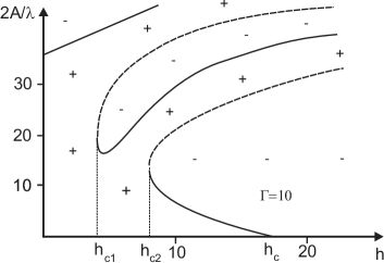
Figure 5: Regions of positive and negative values of the increment coefficient $D_{1}(A,h)$ for $\Gamma=10$. Solid (dashed) lines indicate where the Wigner distribution function for the oscillation amplitude $A$ has a local maximum (minimum) and hence where the stationary state [$D_{1}(A,h)=0]$ is stable (unstable) with respect to small perturbations.

Thus the magnetic shuttle device acts in "opposite" way as compared to electromechanical one. A particularly transparent picture of how spintro-mechanics affects shuttle vibrations emerges in the limit of weak magnetic field $H$ and large electron tunnelling rate $\Gamma_{S(D)}$ between dot and source- and drain electrodes. In order to explore this limit, where $\Gamma_{S}\gg\omega\gg(\mu H/\hbar)^{2}/\Gamma_{D}$ and $\omega/2\pi$ is the natural vibration frequency of the dot, we focus first on the total work done by the exchange force $\mathfrak{F}$ as the dot vibrates under the influence of an elastic force only. In the absence of an external magnetic field the dot is in this case occupied by a spin-up electron emanating from the source electrode. This spin is a constant of motion and hence no electrical current through the device is possible since only spin-down states are available in the drain electrode. During the oscillatory motion of the dot the exchange force is therefore always directed towards the source electrode while its magnitude only depends on the position of the dot, $\mathfrak{F}=\mathfrak{F}_{0}(x)$. As a result, no net work is done by the exchange force on the dot. This is because contributions are positive or negative depending on the direction of the dot’s motion and cancel when summed over one oscillation period. A finite amount of work can only be done if the exchange force deviates from $\mathfrak{F}_{0}(x)$ as a result of spin flip processes induced by the external magnetic field. Such a deviation can be viewed as an additional random force $\mathfrak{F}_{H}$ that acts in the opposite direction to $\mathfrak{F}_{0}(x)$. In the limit of large tunneling rate, $\Gamma\gg\mu H/\hbar$, and small vibration amplitude a spin flip occurs with a probability $\propto(\mu H/\hbar)^{2}/(\omega\Gamma_{D})$ during one oscillation period and is instantly accompanied by the tunneling of the dot electron into the drain electrode, thereby triggering the force $\mathfrak{F}_{H}$. The duration of this force is determined by the time $\delta t\sim 1/\Gamma_{S}(x(t))$ it takes for the spin of the dot to be “restored" by another electron tunneling from the source electrode.

The spin-flip induced random force $\mathfrak{F}_{H}=-\mathfrak{F}_{0}(x)$ is always directed towards the drain electrode. Hence, its effect depends on the dot’s direction of motion: as the dot moves away from the source electrode it will be accelerated, while as it moves towards the source it will be decelerated. Since a spin-flip may occur at any point on the trajectory one needs to average over different spin-flip positions in order to calculate the net work done on the dot. The result, which depends on the competition between the effect of spin flips that occur at the same position but with the dot moving in opposite directions, is nonzero because $\delta t$ is different in the two cases. As the dot moves away from the source electrode the tunneling rate to this electrode will decrease while as the dot moves towards the source it will increase. This means that the duration of spin-flip induced acceleration will prevail over the one for deceleration. As a result, in weak magnetic fields, the dot will accelerate with time and one can expect a spintro-mechanical shuttle instability in this limit.

The situation is qualitatively different in the opposite limit of strong magnetic fields, where $\Gamma\ll\mu H/\hbar$ and the spin rotation frequency therefore greatly exceeds the tunneling rates. In this case the quick precession of the electron spin in the dot averages the exchange force to zero if one neglects the small effects of electron tunneling to and from the dot. If one takes corrections due to tunnelling into account (having in mind that the source electrode only supplies spin-up electrons) one comes to the conclusion that the average spin on the dot will be directed upwards. This results in a net spintro-mechanical force in the direction opposite to that of the net force occurring in a weak magnetic field limit. As a result, in strong magnetic fields one expects on the average a deceleration of the dot. Therefore, there will be no shuttle instability for such magnetic fields.

As we have discussed above spin-flip assisted electron tunnelling from source to dot to drain in our device results in a magnetic exchange force that attracts the dot to the source electrode. It is interesting to note that this is contrary to the effect of the Coulomb force in the same device. Indeed, since the Coulomb force depends on the electric charge of the dot it repels the dot from the source electrode. Hence, while the dot is empty as the result of a spin-flip assisted tunneling event from dot to drain, an “extra" attractive Coulomb force $\mathfrak{F}_{Q}$ is active. An analysis fully analogous with our previous analysis of the “extra" repulsive magnetic exchange force $\mathfrak{F}_{H}$ leads to the conclusion that the effect of the Coulomb force will be just the opposite to that of the exchange force. This means that in the Coulomb blockade regime in the limit of weak magnetic field there is no shuttle instability, while in strong magnetic fields electron shuttling occurs. As was shown the detailed analysis confirms these predictions.

III.5 Mechanically assisted magnetic coupling between nanomagnets

The mechanical force caused by the exchange interaction represents only one effect of the coupling of magnetic and mechanical degrees of freedom in magnetic nanoelectromechanical device. A complementary effect is the of mechanical transportation of magnetization, which we are going to discuss in this subsection.

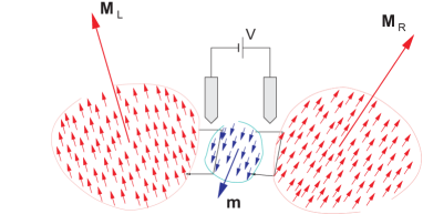
Figure 6: Single-domain magnetic grains with magnetic moments $\textbf{M}_{L}$ and $\textbf{M}_{R}$ are coupled via a magnetic cluster with magnetic moment m, the latter being separated from the grains by insulating layers. The gate electrodes induce an ac electric field, concentrated in the insulating regions. This field, by controlling the heights of the tunnel barriers, affects the exchange magnetic coupling between different components of the system. Reprinted with permission from 8 , L. Y. Gorelik et al., Phys. Rev. Lett. 91, 088301 (2003). $\copyright$ 2003, American Physical Society.

In the magnetic shuttle device presented in Fig. 6, a ferromagnetic dot with total magnetic moment m is able to move between two magnetic leads, which have total magnetization $\textbf{M}_{L,R}$. Such a device was suggested in Ref. 8, in order to consider the magnetic coupling between the leads (which in their turn can be small magnets or nanomagnets) produced by a ferromagnetic shuttle. It is worth to point out that the phenomenon we are going to discuss here has nothing to do with transferring electric charge in the device and it is valid also for a device made of nonconducting material. The main effect, which will be in the focus of our attention, is the exchange interaction between the ferromagnetic shuttle (dot) and the magnetic leads. This interaction decays exponentially when the dot moves away from a lead and hence it is only important when the dot is close to one of the leads. During the periodic back-and-forth motion of the dot this happens during short time intervals near the turning points of the mechanical motion. An exchange interaction between the magnetizations of the dot and a lead results in a rotation of these two magnetization vectors in such a way that the vector sum is conserved. This is why the result of this rotation can be viewed as a transfer of some magnetization $\Delta\textbf{m}$ from one ferromagnet to the other. As a result the magnetization of the dot experiences some rotation around a certain axis. The total angle $\phi$ of the rotation accumulated during the time when the dot is magnetically coupled to the lead is an essential parameter which depends on the mechanical and magnetic characteristics of the device. The continuation of the mechanical motion breaks the magnetic coupling of the dot with the first lead but later, as the dot approaches the other magnetic lead an exchange coupling is established with this second lead with the result that magnetization which is “loaded" on the dot from the first lead is "transferred" to the this second lead. This is how the transfer of magnetization from one magnetic lead to another is induced mechanically. The transfer creates an effective coupling between the magnetizations of the two leads. Such a non-equilibrium coupling can be efficiently tuned by controlling the mechanics of the shuttle device. It is particularly interesting that the sign of the resulting magnetic interaction is determined by the sign of $\cos(\phi/2)$. Therefore, the mechanically mediated magnetic interaction can be changed from ferromagnetic to anti-ferromagnetic by changing the amplitude and the frequency of mechanical vibrations 8 .

IV Resonance spin-scattering effects. Spin shuttle as a "mobile quantum impurity".

Many-particle effects add additional dimension to the shuttling phenomena. These effects accompany electronic tunneling between the gate electrodes and the moving nanoisland. The common source of many-particle effects is the so called "orthogonality catastrophe" related to multiple creation of electron-hole pairs both with parallel and antiparallel spins Mahan67 ; Anderson67 as a response of electronic gas in the leads to single electron tunneling. The second-order cotunneling processes under strong Coulomb blockade result in effective indirect exchange between the shuttle and the leads. This exchange is the source of strong scattering and the many-particle reconstruction of the electron ensemble in the leads known as the Kondo effect. Various manifestations of the Kondo effect in shuttling are reviewed in this section.

The Kondo effect in electron tunneling close to the unitarity limit manifests itself as a sharp zero bias anomaly in the low-temperature tunneling conductance. Many-particle interactions renormalize the electron spectrum enabling "Abrikosov-Suhl resonances" both for odd gogo and even Pust00 ; Kikoin01 electron occupations. In the latter case the resonance is caused by the singlet-triplet crossover in the ground state (see glasko for a review). In the simplest case of odd occupancy a cartoon of a quantum well and a schematic Density of States (DoS) is shown in Fig. 7. For simplicity we consider a case when the dot is occupied by one electron (as in a SET transistor). The corresponding electronic level in the dot is located at an energy $-E_{d}$, deep beyond the Fermi level of the leads ($\epsilon_{F}$). The dot is in the Coulomb blockade regime, and the corresponding charging energy is denoted as $E_{C}$. The Abrikosov-Suhl resonance Abrikosov ; Suhl ; Hewson at $\epsilon_{F}$ arises due to multiple spin flip scattering, so that the narrow peak in the DoS is related mainly to the spin degrees of freedom (see Fig. 7, upper right panel). The width of this resonance is defined by the unique energy scale, the Kondo temperature $T_{K}$, which determines all thermodynamic and transport properties of the SET device through a one-parametric scaling Hewson . The Breit - Wigner (BW) width $\Gamma$ of the dot level associated with the tunneling of dot electrons to the continuum of levels in the leads, is assumed to be smaller than the charging energy $E_{C}$, providing a condition for nearly integer valency regime.

Building on an analogy with the shuttling experiments of Refs. Kot2004, and erbe, , let us consider a device where an isolated nanomachined island oscillates between two electrodes. The applied voltage is assumed low enough so that the field emission of many electrons, which was the main mechanism of tunneling in those experiments, can be neglected. We emphasize that the characteristic de Broglie wave length associated with the dot should be much shorter than typical displacements allowing thus for a classical treatment of the mechanical motion of the nano-particle. The condition $\hbar\omega_{0}\ll k_{B}T_{K}$, necessary to eliminate decoherence effects, requires for e.g. planar quantum dots with the Kondo temperature $T_{K}\gtrsim 100$ mK, the condition $\omega_{0}\lesssim 1$ GHz for oscillation frequencies to hold; this frequency range is experimentally feasible erbe ; Kot2004 . The shuttling island is then to be considered as a “mobile quantum impurity", and transport experiments will detect the influence of mechanical motion on the differential conductance. If the dot is small enough, then the Coulomb blockade guarantees the single electron tunneling or cotunneling regime, which is necessary for the realization of the Kondo effect GR ; glasko .

The above configuration is illustrated in the lower panel of Fig. 7: the shuttle of nanoscale size is mounted at the tight string. Its harmonic oscillations are induced by external elastic force. Unlike the conventional resonance case (the resonance level belongs not to the moving shuttle but develops as a many-body peak at the Fermi level of the leads. When the shuttle moves between source (S) and drain (D) (see the lower panel of Fig. 7), both the energy $E_{d}$ and the width $\Gamma$ acquire a time dependence. This time dependence results in a coupling between mechanical, electronic and spin degrees of freedom. If a source-drain voltage $V_{sd}$ is small enough ($eV_{sd}\ll k_{B}T_{K}$) the charge degree of freedom of the shuttle is frozen out while spin flips play a very important role in co-tunneling processes. Namely, the Abrikosov-Suhl resonance is viewed as a time-dependent Kondo cloud built up from conduction electrons in the leads dynamically screening moving spin localized at the shuttle. Since the electrons in the cloud contain information about the same impurity, they are mutually correlated. Thus, NEM providing a coupling between mechanical and electronic degrees of freedom introduces a powerful tool for manipulation and control of the Kondo cloud induced by the spin scattering and gives a very promising and efficient mechanism for electromechanical transduction on the nanometer length scale.

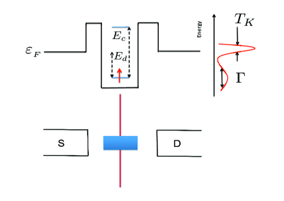
Figure 7: Nanomechanical resonator with spin as a “mobile quantum impurity".

Cotunneling is accompanied by a change of spin projection in the process of charging/discharging of the shuttle and therefore is closely related to the spin/charge pumping problem brouw98 .

A generic Hamiltonian for describing the resonance spin-scattering effects is given by the same Anderson model as above,

$$H_{0}=\sum_{k,\alpha}\varepsilon_{k\sigma,\alpha}a^{\dagger}_{k\sigma,\alpha}a_{k\sigma,\alpha}+\sum_{i\sigma}[E_{d}-eEx]d^{\dagger}_{i\sigma}d_{i\sigma}+E_{C}n^{2}$$

$$H_{tunnel}=\sum_{ik\sigma,\alpha}T^{(i)}_{\alpha}(x)[a^{\dagger}_{k\sigma,\alpha}d_{i\sigma}+H.c],$$ (36)

where ${E}$ is the electric field between the leads. The tunnelling matrix element depends exponentially on the ratio of the time-dependent displacement $x(t)$ and the electronic tunnelling length $\lambda$, see Eq. (15). The time-dependent Kondo Hamiltonian for slowly moving shattle can be obtained by applying a time-dependent Schrieffer-Wolff transformation SW ; KNG00 :

$$H_{K}=\sum_{k\alpha\sigma,k^{\prime}\alpha^{\prime}\sigma^{\prime}}{\cal J}_{\alpha\alpha^{\prime}}(t)[\vec{\sigma}_{\sigma\sigma^{\prime}}\vec{S}+\frac{1}{4}\delta_{\sigma\sigma^{\prime}}]a^{\dagger}_{k\sigma,\alpha}a_{k^{\prime}\sigma^{\prime},\alpha^{\prime}}$$ (37)

where ${\cal J}_{\alpha,\alpha^{\prime}}(t)=\sqrt{\Gamma_{\alpha}(t)\Gamma_{\alpha^{\prime}}(t)/(\pi\rho_{0}E_{d}(t))}$ and $\vec{S}=\frac{1}{2}d_{\sigma}^{\dagger}\vec{\sigma}_{\sigma\sigma^{\prime}}d_{\sigma^{\prime}}$, $\Gamma_{\alpha}(t)=2\pi\rho_{0}|T_{\alpha}(x(t))|^{2}$ are level widths due to tunneling to the left and right leads.

As long as the nano-particle is not subject to an external time-dependent electric field, the Kondo temperature is given by $k_{B}T_{K}^{0}=D_{0}\exp\left[-(\pi E_{C})/(8\Gamma_{0})\right]$ (for simplicity we assumed that $\Gamma_{L}(0)=\Gamma_{R}(0)=\Gamma_{0}$; $D_{0}$ plays the role of effective bandwidth). As the nano-particle moves adiabatically, $\hbar\omega_{0}\ll\Gamma_{0}$, the decoherence effects are small provided $\hbar\omega_{0}\ll k_{B}T_{K}^{0}$.

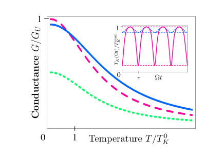
Figure 8: Differential conductance $G$ of a Kondo shuttle for which $\Gamma_{0}$$/$$E_{C}$$=$$0.4$. The solid line denotes $G$ for a shuttle with $\Gamma_{L}$$=$$\Gamma_{R}$, $A$$=$$\lambda$, the dashed line shows $G$ for a static nano-island with $\Gamma_{L}=\Gamma_{R}$, $A$$=$$0$, the dotted line gives $G$ for $\Gamma_{L}$$/$$\Gamma_{R}$$=$$0.5$, $A$$=$$0$. The inset shows the temporal oscillations (here $\Omega\equiv\omega_{0}$) of $T_{K}$ for small $A$$=$$0.05$$\,\lambda$ (dotted line) and large $A$$=$$2.5$$\,\lambda$ (solid line) shuttling amplitudes. Reprinted with permission from kis06 , M. N. Kiselev et al., Phys. Rev. B 74, 233403 (2006). $\copyright$ 2006, American Physical Society.

Let us first assume a temperature regime $T\gg T_{K}$ (weak coupling). In this case we can build a perturbation theory controlled by the small parameter $\rho_{0}{\cal J}(t)\ln[D_{0}/(k_{B}T)]<1$ assuming time as an external parameter. The series of perturbation theory can be summed up by means of a renormalization group procedure Hewson ; KNG00 . As a result, the Kondo temperature becomes oscillating in time:

$$k_{B}T_{K}(t)=D(t)\exp\left[-\frac{\pi E_{C}}{8\Gamma_{0}\cosh(2x(t)/\lambda)}\right].$$ (38)

Neglecting the weak time-dependence of the effective bandwidth $D(t)\approx D_{0}$, we arrive at the following expression for the time-averaged Kondo temperature:

$$\langle T_{K}\rangle=T_{K}^{0}\bigg{\langle}\exp\left[\frac{\pi E_{C}}{4\Gamma_{0}}\frac{\sinh^{2}(x(t)/\lambda)}{1+2\sinh^{2}(x(t)/\lambda)}\right]\bigg{\rangle}.$$ (39)

Here $\langle$$...$$\rangle$ denotes averaging over the period of the mechanical oscillation. The expression (39) acquires an especially transparent form when the amplitude of the mechanical vibrations $A$ is small: $A\lesssim\lambda$. In this case the Kondo temperature can be written as $\langle T_{K}\rangle=T_{K}^{0}\exp(-2W)$, with the Debye-Waller-like exponent $W=-\pi E_{C}\langle x^{2}(t)\rangle)/(8\Gamma_{0}\lambda^{2})$, giving rise to the enhancement of the static Kondo temperature.

The zero bias anomaly (ZBA) in the tunneling conductance is given by

$$G(T)=\frac{3\pi^{2}}{8}G_{0}\Bigg{\langle}\frac{4\Gamma_{L}(t)\Gamma_{R}(t)}{(\Gamma_{L}(t)+\Gamma_{R}(t))^{2}}\frac{1}{[\ln(T/T_{K}(t))]^{2}}\Bigg{\rangle},$$ (40)

where $G_{0}=e^{2}/h$ is a unitary conductance. Although the central position of the island is most favorable for the BW resonance ($\Gamma_{L}=\Gamma_{R}$), it corresponds to the minimal width of the Abrikosov-Suhl resonance. The turning points correspond to the maximum of the Kondo temperature given by the equation (38) while the system is away from the BW resonance. These two competing effects lead to the effective enhancement of $G$ at high temperatures (see Fig. 8).

Summarizing, it was shown in kis06 that Kondo shuttling in a NEM-SET device increases the Kondo temperature due to the asymmetry of coupling at the turning points compared to at the central position of the island. As a result, the enhancement of the differential conductance in the weak coupling regime can be interpreted as a pre-cursor of strong electron-electron correlations appearing due to formation of the Kondo cloud.

Next we turn to the strong coupling regime, $T\ll T_{K}$. We consider this regime for an oscillating cantilever with a nanotip at its end (Fig. 9). Then the motion of a shuttle in $y$ direction is described by the Newton equation which we rewrite in a form

$$\ddot{y}+\frac{\omega_{0}}{Q_{0}}\dot{y}+\omega^{2}_{0}y=\frac{1}{m}F.$$ (41)

where $\omega_{0}=\sqrt{k/m}$ is the oscillator frequency of free cantilever, $Q_{0}$ is the quality factor. $F$ is the Lorentz force acting on moving cantilever in perpendicular magnetic field

$$\vec{F}=L\cdot\vec{I}\times\vec{B}=(0,F,0).$$ (42)

Here $L$ is the length of the cantilever. $\vec{I}$ is the current through the system.

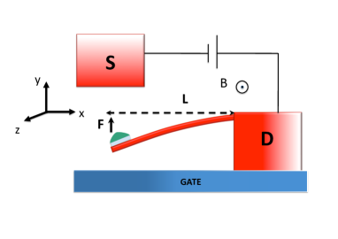
Figure 9: Shuttling quantum dot mounted on a moving metallic pendulum. Magnetic field $B$ is applied along $z$ axis. $\copyright$ 2013, American Physical Society.

In this configuration the Kondo cloud induced by spin scattering is formed both in the immovable part of the setup (drain electrode) and in the oscillating cantilever. The current $\vec{I}$ subject to a constant source-drain bias $V_{sd}$ can be separated in two parts: a dc current associated with a time-dependent dc conductance and an ac current related to the periodic motion of the shuttle. While the dc current is mostly responsible for the frequency shift, the ac current gives an access to the dynamics of the Kondo cloud and provides information about the kinetics of its formation. In order to evaluate both contributions to the total current we rotate the electronic states in the leads in such a way that only one combination of the wave functions is coupled to the quantum impurity. The cotunneling Hamiltonian may be rationalized by means of the Glazman-Raikh rotation, parametrized by the angle $\vartheta_{t}$ defined by the relation $\tan\vartheta_{t}=\sqrt{|\Gamma_{R}(t)/\Gamma_{L}(t)|}$.

Both the ac and dc contributions to the current can be calculated by using Nozière’s Fermi-liquid theory (see Nozieres74 for details). The ac contribution, associated with the time dependence of the Friedel phase $\delta_{\sigma}$ kis12 , is given by

$$\bar{I}_{ac}(t)=\frac{\dot{y}(t)}{\lambda}\frac{eE_{C}}{8\Gamma_{0}}\cdot\frac{eV_{\rm sd}}{k_{B}T_{K}(t)}\cdot\frac{\tanh\left(\frac{2[y(t)-y_{0}]}{\lambda}\right)}{\cosh^{2}\left(\frac{2[y(t)-y_{0}]}{\lambda}\right)}\\$$ (43)

($\exp(4y_{0}/\lambda)=\Gamma_{R}(0)/\Gamma_{L}(0)$). The equation (43) acquires a simple form if we assume that the size of Kondo cloud $R_{K}(y(t))=\hbar v_{F}/(k_{B}T_{K}(y(t)))$ where $v_{F}$ is a Fermi velocity. According to Nozieres Nozieres74 , the Friedel phase $\delta_{\sigma}$ can be Taylor-expanded in the vicinity of its resonance value $\delta_{0\sigma}=\pi/2$ as

$$\delta_{\sigma}(t)=\frac{\pi}{2}+\frac{eV_{\rm sd}R_{K}(y(t))}{\hbar v_{F}}+\frac{g\mu_{B}(\sigma\cdot B)R_{K}(y(t))}{\hbar v_{F}}$$ (44)

and, therefore, $d(\delta_{\uparrow}+\delta_{\downarrow})/dt\propto\dot{y}\cdot dR_{K}(y)/dy$. As a result,

$$\bar{I}_{ac}(t)=2G_{0}V_{\rm sd}\frac{\dot{y}(t)}{v_{F}}\frac{dR_{K}(y)}{dy}.$$ (45)

Thus, the ac current generated in the device due to the mechanical motion of the shuttle contains information about spatial variation of the Kondo cloud.

The "ohmic" dc contribution is fully defined by the adiabatic time-dependence of the Glazman-Raikh angle

$$\bar{I}_{DC}(t)=G_{0}V_{sd}\sin^{2}2\vartheta_{t}\sum_{\sigma}\sin^{2}\delta_{\sigma}$$ (46)

As a result, the ac contribution to the total current can be considered as a first non-adiabatic correction:

$$I_{tot}=I_{ad}(y(t))-\dot{y}\frac{dI_{ad}}{dy}\frac{\hbar\pi E_{C}}{16\Gamma_{0}k_{B}T^{(0)}_{K}}$$ (47)

where $I_{ad}=2\cdot G_{0}\cdot V_{sd}\cosh^{-2}(2[y(t)-y_{0}]/\lambda)$ and $T_{K}^{(0)}$ is the Kondo temperature at the equilibrium position. The small correction to the adiabatic current in (47) may be considered as a first term in the expansion over the small non adiabatic parameter $\omega_{0}\tau\ll 1$, where $\tau$ is the retardation time associated with the inertia of the Kondo cloud. Using such an interpretation one gets $\tau=\hbar\pi E_{C}/(16\Gamma_{0}k_{B}T^{(0)}_{K})$.

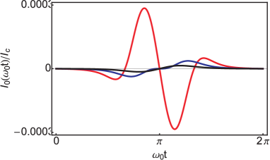
Figure 10: Time dependence of the current $I_{0}$ for different values of asymmetry parameter $u=x_{0}/\lambda$. Here red, blue and black curves correspond to $u=0.5;1.0;1.5;$. For all three curves shuttle oscillates with amplitude $x_{max}=\lambda$, $\hbar\omega_{0}/(k_{B}T_{K}^{\color[rgb]{0,0,0}min\color[rgb]{0,0,0}})=10^{-3}$, $|eV_{\rm bias}|/(k_{B}T_{K}^{\color[rgb]{0,0,0}min\color[rgb]{0,0,0}})=g\mu_{B}B/(k_{B}T_{K}^{\color[rgb]{0,0,0}min\color[rgb]{0,0,0}})=0.1$ with $T_{K}^{(0)}=2K$, $\lambda/L=10^{-4}$. Reprinted with permission from kis12 , M. N. Kiselev et al. Phys. Rev. Lett. 110, 066804 (2013). $\copyright$ 2013, American Physical Society.

Equation (47) allows one to obtain information about the dynamics of the Kondo clouds from an analysis of an experimental investigation of the mechanical vibrations. The retardation time associated with the dynamics of the Kondo cloud is parametrically large compared with the time of formation of the Kondo cloud $\tau_{K}=\hbar/(k_{B}T_{K})$ and can be measured owing to a small deviation from adiabaticity. Also we would like to emphasize a supersensitivity of the quality factor to a change of the equilibrium position of the shuttle characterized by the parameter $u$ (see Fig. 10). The influence of strong coupling between mechanical and electronic degrees of freedom on the mechanical quality factor has been considered in kis12 . It has been shown that both suppression $Q>Q_{0}$ and enhancement $Q<Q_{0}$ of the dissipation of nanomechanical vibrations (depending on external parameters and the equilibrium position of the shuttle) can be stimulated by Kondo tunneling. The latter case demonstrates the potential for a Kondo induced electromechanical instability.

In order to describe these instability, one should discuss the contribution of "Kondo force" $F_{K}$ to the right hand side part (42) of Eq. (41). This force consists of two components Korean :

$$F_{K}=-\frac{\alpha_{K}+\alpha_{\rm ret}}{\cosh^{2}(y-y_{0})\omega_{0}^{2}\lambda}.$$ (48)

where

$$\alpha_{K} = \frac{\pi E_{C}k_{B}T_{K}(t)}{8\Gamma_{0}\lambda},$$ (49)

$$\alpha_{\rm ret} = 2\dot{y}G_{0}V_{\rm bias}BL\tanh(y-y_{0})\tau_{\rm ret}e^{-\beta[1+\tanh(y-y_{0})]/2}$$

Here $\beta=\pi E_{C}/4\Gamma_{0}$ is the coupling strength of electronic states. The first term stems from the Kondo cloud adiabatically following the change of $T_{K}(t)$ induced by the moving shuttle in the source electrode and metallic cantilever. The second term describes the temporal retardation related to dynamics of Kondo cloud with the characteristic time $\tau_{ret}=\hbar\omega_{0}\beta/(2k_{B}T_{K}^{\rm min})$. The time dependent Kondo temperature in the strong coupling limit at $T\ll T_{K}^{min}$ is given by

$$k_{B}T_{k}(t)=k_{B}T_{K}^{min}\exp\left\{\frac{\beta}{2}[1+\tanh(y(t)-y_{0})])\right\}.$$ (50)

The $k_{B}T_{K}^{min}$ plays the role of the cutoff energy for Kondo problem.

The instability is controlled by the bias $V_{\rm bias}$ entering $\alpha_{\rm ret}$. Fig. 11 illustrates two regimes of Kondo shuttling. Namely, at small bias the Kondo force controlled by external fields further damps the oscillator, and we obtain an efficient mechanism of cooling the nano-shuttle. On the other hand, at $V_{\rm bias}$ above some treshold value, the contribution of the Kondo force enhances the oscillations, and we arrive at the non-linear steady state regime of self sustained oscillations.

Summarizing, we emphasize that the Kondo phenomenon in single electron tunneling gives a very promising and efficient mechanism for electromechanical transduction on a nanometer length scale. Measuring the nanomechanical response on Kondo-transport in a nanomechanical single-electron device enables one to study the kinetics of the formation of Kondo-screening and offers a new approach for studying nonequilibrium Kondo phenomena. The Kondo effect provides a possibility for super high tunability of the mechanical dissipation as well as super sensitive detection of mechanical displacement.

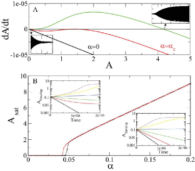
Figure 11: Panel A: Amplitude dynamics at different values of the dimensionless force $\alpha$ (see details in the text). Insets: time trace of the oscillation at two different fixed point indicated by arrow. Panel B: Saturation amplitude as a function of dimensionless force. Different colors denote initial conditions near (black dots) and far (red dots) from the equilibrium position $y_{0}$. Insets: amplitude envelope as a function of dimensionless time calculated by using Eq. (49). The parameter $\alpha$ varies from $\alpha=0$ (black) to $\alpha=0.1$ (magenta). The equations are solved for the following set of parameters: $\beta=8$, $\gamma=10^{-5}$, $y_{0}=0.5$ and $\frac{\hbar\omega_{0}}{k_{B}T_{K}^{min}}=10^{-3}$. Reprinted with permission from kis12 , T. Song et al., New Journal of Physics, 16, 033043 (2014).

V Conclusions

During the last several years there has been significant activity in the study of nanoelectromechanical (NEM) shuttle structures. In this review we concentrate on description of the influence of spin-related effects on the functionality of shuttle devices. In particular, we emphasize the importance of electronic spin in shuttle devices made of magnetic materials. Spin-dependent exchange forces can be responsible for a qualitatively new nanomechanical performance opening a new field of study that can be called spintro-mechanics. Electronic many-body effects, appearing beyond the weak tunneling approach, result in single electron shuttling assisted by Kondo-resonance electronic states. The possibility to achieve a high sensitivity to coordinate displacement in electromechanical transduction along with the possibility to study the kinetics of the formation of many-body Kondo states has also been demonstrated.

There are still a number of unexplored shuttling regimes and systems, which one could focus on in the nearest future. In addition to magnetic shuttle devices one could explore hybrid structures where the source/drain and gate electrodes are hybrids of magnetic and superconducting materials. Then one could expect spintromechanical actions of a supercurrent flow as well as superconducting proximity effects in the spin dynamics in magnetic NEM devices. An additional direction is the study of shuttle operation under microwave radiation. In this respect microwave assisted spintromechanics is of special interest due to the possibility of microwave radiation to resonantly flip electronic spins. As in ballistic point contacts such flips can be confined to particular locations by the choice of microwave frequency, allowing for external tuning of the spintromechanical dynamics of the shuttle.

VI Acknowledgements

Financial support from the Swedish VR, and the Korean WCU program funded by MEST/NFR (R31-2008-000-10057-0) is gratefully acknowledged. This research was supported in part by the Project of Knowledge Innovation Program (PKIP) of Chinese Academy of Sciences, Grant No. KJCX2.YW.W10. I. V. K. and A. V. P. acknowledge financial support from the National Academy of Science of Ukraine (grant No. 4/13-N). I. V. K. thanks the Department of Physics at the University of Gothenburg for hospitality.

References

- (1) R. I. Shekhter, Zh. Eksp. Teor. Fiz. 63, 1410 (1972) [ Sov. Phys. JETP 36, 747 (1972)]; I. O. Kulik and R. I. Shekhter, Zh. Eksp. Teor. Fiz. 68, 623 (1975) [ Sov. Phys. JETP 41, 308 (1975)]
- (2) R. I. Shekhter, Y. Galperin, L. Y. Gorelik, A. Isacsson, and M. Jonson, J. Phys.: Condens. Matter 15, R441 (2003).
- (3) R. I. Shekhter, L. Y. Gorelik, M. Jonson, Y. M. Galperin, and V. M. Vinokur, J. Compt. Theoret. Nanoscience 4, 860 (2007).
- (4) R. I. Shekhter, F. Santandrea, G. Sonne, L. Y. Gorelik, and M. Jonson, Fiz. Nizk. Temp. 35, 841 (2009) [Low Temp. Phys. 35, 662 (2009)].
- (5) M. Blencowe, Phys. Rep. 395, 159 (2004).
- (6) K. C. Schwab and M. L. Roukes, Phys. Today 58, 36 (2005).
- (7) K. L. Ekinci and M. L. Roukes, Rev. Sci. Instrum. 76, 061101 (2005).
- (8) A. N. Cleland, Foundations of Nanomechanics (Springer-Verlag, New York, 2003).
- (9) M. Poot and H. S. J. van der Zant, Phys. Rep. 511, 273 (2012).
- (10) L. Y. Gorelik, A. Isacsson, M. V. Voinova, B. Kasemo, R. I. Shekhter, and M. Jonson, Phys. Rev. Lett. 80, 4526 (1998).
- (11) L. M. Jonson, L. Y. Gorelik, R. I. Shekhter, and M. Jonson, Nano Lett. 5, 1165 (2005).
- (12) D. Fedorets, L. Y. Gorelik, R. I. Shekhter, and M. Jonson, Europhys. Lett. 58, 99 (2002).
- (13) D. Fedorets, L. Y. Gorelik, R. I. Shekhter, and M. Jonson, Phys. Rev. Lett. 92, 166801 (2004).
- (14) T. Novotny, A. Donarini, and A.-P. Jauho, Phys. Rev. Lett. 90, 256801 (2003).
- (15) D. Fedorets, Phys. Rev. B 68, 033106 (2003).
- (16) R. Hansen, L. P. Kouwenhoven, J. R. Petta, S. Tarucha, and L. M. K. Vandersypen, Rev. Mod. Phys. 79, 1217 (2007).
- (17) K. C. Nowak, F. H. L. Koppens, Yu. V. Nazarov, and L. M. K. Vandersypen, Science 318, 1430 (2007).
- (18) S. Foletti, H. Bluhm, D. Mahalu, V. Umansky, A. Yacoby, Nat. Phys. 318, 1430 (2007).
- (19) F. Jelezko, T. Gaebel, I. Popa, A. Gruber, and J. Wrachtrup, Phys. Rev. Lett. 92, 076401 (2004).
- (20) A. Kadigrobov, Z. Ivanov, T. Claeson, R.I. Shekhter, M. Jonson, Euro Phys. Lett. 67, 948 (2004).
- (21) D. Press, T. D. Ladd, B. Zhang, and Y. Yamamoto, Nature 456, 218 (2008).
- (22) B. M. Chernobrod, G P. Berman, J. Appl. Phys. 97, 014903 (2005).
- (23) P. Rabl, S. Kolkowitz, F. Koppens, J. Harris, P. Zoller, and M. Lukin, Nat. Phys. 6, 602 (2010).
- (24) G. Balasubramanian, I. Y. Chan, R. Kolesov, M. Al-Hmoud, J. Tisler, C. Shin, C. Kim, A. Wojcik, P. R. Hemmer, A. Krueger, T. Hanke, A. Leitenstorfer, R. Bratschitsch, F. Jelezko, and J. Wrachtrup, Nature 455, 648 (2008).
- (25) J. R. Maze, P. L. Stanwix, J. S. Hodges, S. Hong, J. M. Taylor, P. Cappellaro, L. Jiang, M. V. Gurudev Dutt, E. Togan, A. S. Zibrov, A. Yacoby, R. L. Walsworth, and M. D. Lukin, Nature 455, 644 (2008).
- (26) J. M. Taylor, P. Cappellaro, L. Childress, L. Jiang, D. Budker, P. R. Hemmer, A. Yacoby, R. Walsworth, and M. D. Lukin, Nat. Phys. 4, 810 (2008).
- (27) D. Rugar, R. Budakian, H. J. Mamin, and B. W. Chui Nature 430, 329 (2004).
- (28) S. Hong, M. S. Grinolds, P. Maletinsky, R. L. Walsworth, M. D. Lukin, and A. Yacoby, Nano Lett. 12, 3920 (2012).
- (29) F. May, M. R. Wegewijs, and W. Hofstetter, Beilstein J. Nanotechnol. 2, 693 (2011).
- (30) D. A. Ruiz-Tijerina, P. S. Cornaglia, C. A. Balseiro, and S. E. Ulloa, Phys. Rev. B 86, 035437 (2012).
- (31) J. Fransson and J.-X. Zhu, Phys. Rev. B 78, 133307 (2008).
- (32) F. Reckermann, M. Leijnse, and M. R. Wegewijs, Phys. Rev. B 79, 075313 (2009).
- (33) P. Rabl, P. Cappellaro, M. V. Gurudev Dutt, L. Jiang, J. R. Maze, and M. D. Lukin Phys. Rev. B 79, 041302 (2009).
- (34) S. D. Bennett, S. Kolkowitz, Q. P. Unterreithmeier, P. Rabl, A. C. Bleszynski Jayich, J. G. E. Harris, and M. D. Lukin, arXiv: 1205.6740 (unpublished).
- (35) D. A. Garanin and E. M. Chudnovsky, Phys. Rev. X 1, 011005 (2011).
- (36) C. L. Degen, M. Poggio, H. J. Mamin, and D. Rugar, Phys. Rev. Lett. 100, 137601 (2008).
- (37) G. P. Berman, V. N. Gorshkov, D. Rugar, and V. I. Tsifrinovich, Phys. Rev. B 68, 094402 (2003).
- (38) A. Pa’lyi, P. R. Struck, M. Rudner, K. Flensberg, and G. Burkard, Phys. Rev. Lett. 108, 206811 (2012).
- (39) C. Ohm, C. Stampfer, J. Splettstoesser, and M. Wegewijs, Appl. Phys. Lett. 100,143103 (2012).
- (40) Zhao Nan, Zhou Duan-Lu, Zhu Jia-Lin Commun. Theor. Phys. 50,1457 (2008).
- (41) L. Y. Gorelik, S. I. Kulinich, R. I. Shekhter, M. Jonson, V. M. Vinokur, Phys. Rev. B71, 03527 (2005).
- (42) Colossal Magnetoresistive Oxides, edited by Y. Tokura (Gordon and Breach Science Publishers, Amsterdam, 2000).
- (43) J. Z. Sun, W. J. Gallagher, P. R. Duncombe, L. Krusin-Elbaum, R. A. Altman, A. Gupta, Yu Lu, G. Q. Gong, and Gang Xiao, Appl. Phys. Lett. 69, 3266 (1996).
- (44) J. Z. Sun, L. Krusin-Elbaum, P. R. Duncombe, A. Gupta, and R. B. Laibowitz, Appl. Phys. Lett. 70, 1769 (1997).
- (45) J. Z. Sun, Y. Y. Wang, and V. P. Dravid, Phys. Rev. B 54, R8357 (1996).
- (46) T. Kimura, Y. Tomioka, H. Kuwahara, A. Asamitsu, M. Tamura, and Y. Tokura, Science 274, 1698 (1996).
- (47) L. Y. Gorelik, S. I. Kulinich, R. I. Shekhter, M. Jonson, and V. M. Vinokur, Phys. Rev. Lett. 95,116806 (2005).
- (48) L. Y. Gorelik, S. I. Kulinich, R. I. Shekhter, M. Jonson, and V. M. Vinokur, Low Temp. Phys. 33,757 (2007).
- (49) L. Y. Gorelik, S. I. Kulinich, R. I. Shekhter, M. Jonson, and V. M. Vinokur, Appl. Phys. Lett. 90,192105 (2007).
- (50) L. Y. Gorelik, S. I. Kulinich, R. I. Shekhter, M. Jonson, and V. M. Vinokur, Phys. Rev. B 77,174304 (2008).
- (51) D. Fedorets, L. Y. Gorelik, R. I. Shekhter, and M. Jonson, Phys. Rev. Lett. 95, 057203 (2005).
- (52) L. Y. Gorelik, D. Fedorets, R. I. Shekhter, and M. Jonson, New J. Phys. 7, 242 (2005).
- (53) S.I.Kulinich, L.Y.Gorelik, A.N.Kalinenko, I.V.Krive, R.I.Shekhter, Y.W.Park,and M.Jonson, Phys. Rev. Lett. 112, 117206 (2014).
- (54) D. Radic, A. Nordenfelt, A. M. Kadigrobov, R. I. Shekhter, M. Jonson, and L. Y. Gorelik, Phys. Rev. Lett. 107, 236802 (2011).
- (55) G. Binash, P. Grünberg, F. Saurenbach, and W. Zinn, Phys. Rev. B 39, 4828 (1989).
- (56) E. Y. Tsymbal, O. N. Mryasov, and P. R. LeClair, J. Phys.: Condens. Matter 15, R109 (2003).
- (57) K. Tsukagoshi, B. W. Alphenaar, and H. Ago, Nature 401, 572 (1999).
- (58) R. Thamankar, S. Niyogi, B. Y. Yoo, Y. W. Rheem, N. V. Myung, R. C. Haddon, and R. K. Kawakami, Appl. Phys. Lett. 89, 033119 (2006).
- (59) R. I. Shekhter, A. Pulkin, and M Jonson, Phys. Rev. B 86, 100404 (2012).
- (60) J. Koch, and F. von Oppen Phys. Rev. Lett. 94, 206804 (2005); J. Koch, F. von Oppen, and A. V. Andreev, Phys. Rev. B 74, 205438 (2006) .
- (61) M. Galperin, M. A. Ratner, and A. Nitzan, J. Phys.: Cond. Matter 19, 103201 (2007).
- (62) B. Zebli, H. A. Vieyra, I. Carmeli, A. Hartschuh, J. P. Kotthaus, A. W. Holleitner, Phys. Rev. B 79, 205402 (2009).
- (63) D. W. Pang, F.-W. Yuan, Y.-C. Chang, G.-A. Li, and H.-Y. Tuan, Nanoscale 4, 4562 (2012).
- (64) L. Y. Gorelik, R. I. Shekhter, V. M. Vinokur, D. E. Feldman, V. I. Kozub, and M. Jonson, Phys. Rev. Lett. 91, 088301 (2003).
- (65) G.D. Mahan, Phys. Rev. 153, 882 (1967); Phys. Rev. 163, 612 (1967)
- (66) P.W.Anderson, Phys. Rev. Lett. 34, 953 (1967).
- (67) D. Goldhaber-Gordon, H. Shtrikman, D. Mahalu, D. Abush-Magder, U. Meirav, M. A. Kastner, Nature 391, 156 (1998); S. M. Cronenwett, T. H. Oosterkamp, and L. P. Kouwenhoven, Science 281, 540 (1998).
- (68) M. Pustilnik, Y. Avishai, and K. Kikoin, Phys. Rev. Lett. 84, 1756 (2000).
- (69) K. Kikoin, and Y. Avishai, Phys. Rev. Lett. 86, 2090 (2001); Phys. Rev. B 65, 115329 (2002).
- (70) M. Pustilnik and L. I. Glazman, J. Phys.: Condens. Matter 16, R513 (2004).
- (71) A. A. Abrikosov, Physics 2, 21 (1965).
- (72) H. Suhl, Physics 2, 39 (1965); Phys. Rev. 138, A515 (1965).
- (73) A. C. Hewson, The Kondo problem to Heavy Fermions, Cambridge University Press, Cambridge (1993).
- (74) D. V. Scheible, C. Weiss, J. P. Kotthaus, and R. H. Blick, Phys. Rev. Lett. 93, 186801 (2004); D. V. Scheible and R. H. Blick, Appl. Phys. Lett. 84, 4632 (2004).
- (75) A.Erbe, C. Weiss, W. Zwerger, and R. H. Blick, Phys. Rev. Lett. 87, 096106 (2001).
- (76) L. I. Glazman and M. E. Raikh, Pis’ma Zh. Eksp. Theor. Fiz. 47, 378 (1988) [JETP Lett. 47, 452 (1988)];
- (77) P. W. Brouwer, Phys.Rev. B58, R10135 (1998);P. Sharma and P. W. Brouwer, Phys. Rev. Lett. 91, 166801 (2003); T. Aono, Phys. Rev. Lett. 93, 116601 (2004).
- (78) J. R. Schrieffer and P. A. Wolf, Phys. Rev. 149, 491 (1966).
- (79) A. Kaminski, Yu.V. Nazarov, and L.I. Glazman, Phys. Rev. B 62, 8154 (2000).
- (80) M. N. Kiselev, K. Kikoin, R. I. Shekhter, and V. M. Vinokur, Phys. Rev. B 74, 233403 (2006)
- (81) P. Nozières, J. Low Temp. Phys. 17, 31 (1974).
- (82) M. N. Kiselev, K. Kikoin, L. I. Gorelik, and R. I. Shekhter, Phys. Rev. Lett. 110, 066804 (2013).
- (83) T. Song, M.N. Kiselev, K. Kikoin, R.I. Shekhter, and L.Y. Gorelik, New Journal of Physics 16, 033043 (2014).