Accelerated Randomized Benchmarking

Abstract

Quantum information processing offers promising advances for a wide range of fields and applications, provided that we can efficiently assess the performance of the control applied in candidate systems. That is, we must be able to determine whether we have implemented a desired gate, and refine accordingly. Randomized benchmarking reduces the difficulty of this task by exploiting symmetries in quantum operations.

Here, we bound the resources required for benchmarking and show that, with prior information, we can achieve several orders of magnitude better accuracy than in traditional approaches to benchmarking. Moreover, by building on state-of-the-art classical algorithms, we reach these accuracies with near-optimal resources. Our approach requires an order of magnitude less data to achieve the same accuracies and to provide online estimates of the errors in the reported fidelities. We also show that our approach is useful for physical devices by comparing to simulations.

Our results thus enable the application of randomized benchmarking in new regimes, and dramatically reduce the experimental effort required to assess control fidelities in quantum systems. Finally, our work is based on open-source scientific libraries, and can readily be applied in systems of interest.

Quantum information processing devices offer great promise in a variety of different fields, including chemistry and material science, data analysis and machine learning  Wiebe et al. (2012, 2014a); Kassal et al. (2011); Hastings et al. (2014), as well as cryptography Shor (1995). Over the past few years, proposals have been advanced for quantum information processing past the classical scale, based on node-based architectures Nickerson et al. (2014); Borneman et al. (2012). In addition, rapid progress has been made towards experimental implementations that might allow for developing such devices Chow et al. (2014); Barends et al. (2014). An impediment in this effort, however, is presented by the difficulty of calibrating and diagnosing quantum devices.

In particular, in the development of quantum information processing, an important experimental challenge is to efficiently characterize the quality with which we can control a quantum system. By characterizing the quality of a quantum gate that is implemented by a control pulse, we can then reason about the utility of that gate for quantum information processing tasks. For instance, we can estimate the feasibility of and the resources required to implement error correction using that control by comparing to proven and numerically estimated fault-tolerance thresholds Gottesman (2009); Fowler et al. (2009), or can adjust our control sequences to account for differences between our control model and the actual system.

In cases where only the quality of a quantum gate or set of gates is required, randomized benchmarking has proven to be a useful means of extracting this information with relatively little experimental effort Magesan et al. (2012a), has been demonstrated in a variety of experimental settings Ryan et al. (2009); Chow et al. (2009); Olmschenk et al. (2010); Brown et al. (2011); Moussa et al. (2012); Tan et al. (2013); Córcoles et al. (2013); Barends et al. (2014). Randomized benchmarking has also been used to improve gate fidelities by characterizing cross-talk Gambetta et al. (2012) or distortions Gustavsson et al. (2013). Extracting fidelity information can often be useful in diagnosing performance and problems with a device in lieu of full characterization Kelly et al. (2014). Moreover, randomized benchmarking has also been used to extract information about the completely positive and unital parts of linear maps Kimmel et al. (2014).

Here, using near-optimal data processing together with prior information, we accelerate the data processing used in benchmarking experiments, such that to achieve the accuracy demanded of benchmarking protocols, we require orders of magnitude less experimental data. We also extend results on the achievable estimation quality in the presence of finite sampling Epstein et al. (2014) and prior information, then show that our accelerated methods are nearly optimal. Our data processing methods also provide estimates of their own performance, such that our approach thus enables randomized benchmarking to be used where data collection costs make existing benchmarking protocols impractical. Thus, our work complements recent results on the robustness of randomized benchmarking Wallman and Flammia (2014) to provide an experimentally useful tool.

Randomized benchmarking has been recently used to adaptively calibrate control designed by optimal control theory methods such as GRAPE Khaneja et al. (2005), allowing for differences between the control model and the actual system to be adjusted for in experimental practice Egger and Wilhelm (2014). These methods are applied in a control design and calibration step, however, and do not allow for control for to be recalibrated dynamically. Whereas randomized benchmarking is performed at the inner-loop of current control calibration algorithms Kelly et al. (2014), any data collection overhead in benchmarking becomes a very significant cost to control calibration as a whole. Thus, by reducing the data requirements using both better fitting methods and strong prior information, we can enable new applications, such as extending control calibration to an online context.

Here, we show that by using prior information together with the sequential Monte Carlo (SMC) parameter estimation algorithm, we can obtain very accurate estimates even in the limit of one bit of data per sequence length, using instead a variety of sequence lengths to probe the performance of our gate set. We also show that for gates with fidelities near unity, increasing the length of benchmarking sequences offers little compared to repeating experiments at already optimal sequence lengths. The SMC algorithm is based on Bayesian methods, which have been used successfully in a variety of quantum information processing tasks Schirmer and Langbein (2010); Schirmer and Oi (2009); Huszár and Houlsby (2012); Sergeevich et al. (2011); Ferrie et al. (2013); Shulman et al. (2014); Combes et al. (2014). SMC has recently been used in quantum information to learn states Huszár and Houlsby (2012) and Hamiltonians Granade et al. (2012a); Stenberg et al. (2014), and to provide robust error bounds on inferred parameters Ferrie (2014). The primary cost incurred by the SMC algorithm is that the data must be simulated repeatedly; though this can be mitigated by using quantum resources Wiebe et al. (2014b, c, d). Here we show that since the symmetries afforded by random benchmarking experiments can be used to simulate datasets with costs that are constant with respect to the dimension of the Hilbert space of interest Magesan et al. (2012a), SMC can be implemented with little overhead. Thus, randomized benchmarking mitigates the primary disadvantage of SMC by removing the need to simulate the quantum system.

Moreover, the method of hyperparameters Granade et al. (2012a) generalizes our approach to allow gate fidelities to be non-trivial functions of some other parameter of interest, such that the underlying parameter is learned directly. This approach is especially relevant if, for example, the effect of the unknown hyperparameter depends on an experimental choice, such that distinct benchmarking experiments can be used in concert in a straightforward way.

Our work proceeds first by defining the benchmarking model that we use, then showing bounds on the estimation of the parameters of this model using the Cramer-Rao bound. We then apply sequential Monte Carlo to the benchmarking model and compare to the performance of traditional methods, and to the optimal performance achievable with prior information, showing that our method offers distinct advantages, and is nearly optimal.

I Interpretation of Likelihood as Marginalization

Magesan et al Magesan et al. (2012a) showed that the average fidelity $F_{g}$ taken over all randomized benchmarking sequences of a given length can be expressed in terms of the survival probability

$$\Pr(\text{survival}|\psi,\vec{i}_{m})=\mathrm{Tr}[E_{\psi}\mathchoice{\hat{\vphantom{\rule{1.0pt}{6.14584pt}}\smash{\hat{S}}}}{\hat{\vphantom{\rule{1.0pt}{6.14584pt}}\smash{\hat{S}}}}{\hat{\vphantom{\rule{1.0pt}{6.46875pt}}\smash{\hat{S}}}}{\hat{\vphantom{\rule{1.0pt}{6.92082pt}}\smash{\hat{S}}}}_{\vec{i}_{m}}(\rho_{\psi})],$$ (1)

where $E_{\psi}$ is a measurement effect corresponding to a fiducial state $\rho_{\psi}$, and where $\mathchoice{\hat{\vphantom{\rule{1.0pt}{6.14584pt}}\smash{\hat{S}}}}{\hat{\vphantom{\rule{1.0pt}{6.14584pt}}\smash{\hat{S}}}}{\hat{\vphantom{\rule{1.0pt}{6.46875pt}}\smash{\hat{S}}}}{\hat{\vphantom{\rule{1.0pt}{6.92082pt}}\smash{\hat{S}}}}_{\vec{i}_{m}}=\mathchoice{\hat{\vphantom{\rule{1.0pt}{6.14584pt}}\smash{\hat{S}}}}{\hat{\vphantom{\rule{1.0pt}{6.14584pt}}\smash{\hat{S}}}}{\hat{\vphantom{\rule{1.0pt}{6.46875pt}}\smash{\hat{S}}}}{\hat{\vphantom{\rule{1.0pt}{6.92082pt}}\smash{\hat{S}}}}_{i_{m}}\circ\cdots\circ\mathchoice{\hat{\vphantom{\rule{1.0pt}{6.14584pt}}\smash{\hat{S}}}}{\hat{\vphantom{\rule{1.0pt}{6.14584pt}}\smash{\hat{S}}}}{\hat{\vphantom{\rule{1.0pt}{6.46875pt}}\smash{\hat{S}}}}{\hat{\vphantom{\rule{1.0pt}{6.92082pt}}\smash{\hat{S}}}}_{i_{1}}$ is the superoperator representing the sequence $\vec{i}_{m}$. In particular, the expectation value of this survival probability over all sequences of a given length $m$ was shown to produce the uniform-average fidelity

$$F_{g}(m,\psi)=\mathbb{E}_{\vec{i}_{m}|m}[\Pr(\text{survival}|\psi,\vec{i}_{m})]=\Pr(\text{survival}|\psi,m).$$ (2)

We may thus interpret the fidelity averaged over a unitary design as a probability of survival in an experiment in which we do not know the sequence being performed. As discussed in detail in Appendix A, if sequences are fairly drawn from the 2-design independently of all other experimental choices, then this is a valid assumption, such that the marginalized survival probability can be taken as the likelihood for our randomized benchmarking model. Note that in the remainder of the paper, we will let $\psi$ be fixed, and will drop the notation conditioning on this assumption.

Using the expansion of the marginalized survival $F_{g}(m)$ given by Magesan et al Magesan et al. (2012a), we can rewrite the likelihood in a way that explicitly depends on the parameters of interest, and that no longer requires simulating the quantum dynamics of the system. Thus, we can use Bayesian methods without simulating the system under study. In particular, we consider the zeroth-order model

$$F_{g}(m)=A_{0}p^{m}+B_{0}$$ (3)

for parameters $A_{0}$, $B_{0}$ and $p$ given by

$$A_{0} :=\mathrm{Tr}\left[E_{\psi}\Lambda\left(\rho_{\psi}-\frac{\mathbbm{1}}{d}\right)\right]$$ (4a)

$$B_{0} :=\mathrm{Tr}\left[E_{\psi}\Lambda\left(\frac{\mathbbm{1}}{d}\right)\right]$$ (4b)

$$p :=(dF_{\mathrm{ave}}-1)/(d-1),$$ (4c)

and where $F_{\mathrm{ave}}$ is the fidelity of the average channel $\Lambda=\mathbb{E}_{i,j}[\Lambda_{i,j}]$, taken over time steps $i$ and elements of the gate set $j$. By these definitions, for ideal preparation, evolution and measurement, $A_{0}=1-\frac{1}{d}$ and $B_{0}=\frac{1}{d}$. Since we will often use the example of a qubit, we thus have that the ideal $A_{0}=B_{0}=1/2$. A sketch of the derivation of this model is given in Figure 1. The interpretation of first- and higher-order models follows in a similar manner. Since we use the zeroth-order model as an example in this work, we will drop the subscript-$0$ for brevity.

Figure 1: Sketch of Magesan et al derivation of the zeroth-order model Magesan et al. (2012a). (a) Sequence of length $m=3$ Clifford operations. (b) Change of variables to $V_{i}$, factoring out previous gates $U_{i-1}$, and with the base case $U_{1}=V_{1}$. The $V$ gates then form a 2-design. (c) Expectation value over random gates in (a) and (b), giving the twirling superchannel $W$ acting on $\Lambda$.

Because the fidelity of a channel is invariant under Clifford twirling, the parameter $p$ represents the strength of the depolarizing channel of fidelity $F_{\mathrm{ave}}$ produced by twirling the average channel $\Lambda$, and can be used to recover $F_{\mathrm{ave}}$. Similarly, in the interleaved protocol Magesan et al. (2012b), we consider two probabilities, $p_{\text{ref}}$ and $p_{\bar{\mathcal{C}}}$, respectively representing the sequences with $m$ random Clifford gates multiplied together, or interleaved with some gate $\mathcal{C}$ under study. From these probabilities, we can extract the referenced probability of gate error $\tilde{p}\mathrel{:=}p_{\mathrm{ref}}/p_{\bar{\mathcal{C}}}$. Each of $p_{\mathrm{ref}}$ and $p_{\bar{\mathcal{C}}}$ is traditionally extracted from a fit to the zeroth- or first-order model .

II Achievable Accuracy

We now consider only the interleaved model since it is more general. For brevity, we represent the model by a vector $\vec{x}=(\tilde{p},p_{\text{ref}},A,B)$, so that the likelihood function for the interleaved model is

$$\Pr(1|\vec{x};m,\text{mode})=\begin{cases}Ap_{\text{ref}}^{m}+B&\text{mode is reference}\\ A(p_{\text{ref}}\tilde{p})^{m}+B&\text{mode is interleaved}\end{cases}$$ (5)

where we have labeled the survival event by “1” to more easily allow for using binomial distributions to consider sums over multiple measurements of the same sequence length.

Having defined our model, it is critical to account for the accuracy with which we can estimate the parameters using finite data records. Here, we extend the results of Epstein et al Epstein et al. (2014) by explicitly calculating the Fisher information of $\Pr(1|\vec{x})$. We can find a bound on the achievable estimation error in this model by appealing to the Cramér-Rao Bound Cover and Thomas (2006), which states that the Fisher information matrix $\matr{I}(\vec{x})$ bounds the error matrix $\matr{E}(\vec{x})$ of any unbiased estimator $\hat{\vec{x}}$ by the inequality

$$\vec{E}(\vec{x}):=\mathbb{E}_{D|\vec{x}}[(\hat{\vec{x}}(D)-\vec{x})(\hat{\vec{x}}(D)-\vec{x})^{\mathrm{T}}]\geq\matr{I}(\vec{x})^{-1}.$$ (6)

If the Fisher information matrix is singular, as is the case here when all of the measured sequences are of the same length, the inverse is taken to be the Moore-Penrose pseudo-inverse. With at least four different sequence lengths, however, we can break the degeneracy. Since this number depends on the dimension of the model and not the underlying Hilbert space, only four measurements are required to break the degeneracy, even for systems of higher dimension than qubits.

It is often the case that we are only interested in $\tilde{p}$, the survival probability, and hence the gate fidelity, of a particular gate Ryan et al. (2009). In this case, we can bound the error of only that parameter by looking at a single element of the error and Fisher information matrix as

$$\vec{E}(\vec{x})_{\tilde{p},\tilde{p}}\geq 1/\vec{I}(\vec{x})_{\tilde{p},\tilde{p}}.$$ (7)

Figure 2: Optimal value of $m$ as a function of the scale $A$ and offset $B$ parameters, with $\tilde{p}=0.9988$ and $p_{\mathrm{ref}}=0.9978$, based on the example of Barends et al. (2014). On the top left, $B=0.5$. On the top right, $A$ = 0.25. Below, we take the limit as $d\to\infty$ of $\lceil m_{\text{opt}}\rceil$, assuming $\tilde{F}=F_{\mathrm{ref}}=F$.

To find the Fisher information for randomized benchmarking, we derive the Fisher score $\vec{q}$ of this model, conditioned on $1$,

$$\begin{aligned} \vec{q}(\vec{x}|1;m,\text{mode})&=\nabla_{\vec{x}}\log\Pr(1|\vec{x};m,\text{mode})\\ &=\Pr(1|\vec{x};m,\text{mode})^{-1}\begin{cases}(0,\,Amp_{\text{ref}}^{m-1},\,p_{\text{ref}}^{m},\,1)&\text{reference}\\ (Am\tilde{p}^{m-1}p_{\text{ref}}^{m},\,Am\tilde{p}^{m}p_{\text{ref}}^{m-1},\,p_{\text{ref}}^{m},\,1)&\text{interleaved}\end{cases},\end{aligned}$$ (8)

where the similar expression for the outcome “0” follows immediately. With this, we can calculate the Fisher information matrix $\vec{I}(\vec{x}):=\mathbb{E}_{D|\vec{x}}[\vec{q}(\vec{x}|D)\vec{q}(\vec{x}|D)^{\rm T}]$, where $D$ labels the outcomes.

Fisher information analysis is one of the most powerful tools of statistical analysis since it bounds the performance of the continuous infinity of possible estimators we could choose. However, given the difficulty of analytically computing the inverse of sums over Fisher information matrices of this form, we use numerical methods for its evaluation. In particular, QInfer Granade et al. (2012b) performs this calculation automatically, given an implementation of (8).

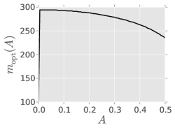
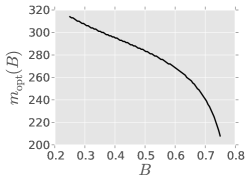
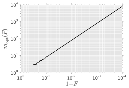
In experimentally relevant regimes, the task is to gain further accuracy when it is known a priori that the fidelity is high. To minimize the error in estimating $\tilde{p}$, we maximize the corresponding element of the Fisher information matrix. Note that, as is shown in Figure 2, this optimum depends strongly on the value of $A$ and $B$ when $\tilde{p},p_{\mathrm{ref}}\approx 1$. For ideal measurements and unital channels, as $d\to\infty$ we have $B\to 0$ and $A\to 1$ such that for large systems,

$$\lim_{d\to\infty}m_{\text{opt}}\approx\frac{1}{1-\tilde{F}F_{\mathrm{ref}}}.$$ (9)

As shown in Figure 2, this can grow large for $|1-F|\to 0$, but even for fidelities near thresholds, such as $|1-F|\approx 10^{-3}$ as considered by Barends et al. (2014), $m_{\text{opt}}$ remains manageable at about 500.

The above calculation is relevant in scenarios where the parameters not of interest (that is, $A$ and $B$) are known fairly well and the gate fidelity is already known to be near unity. If we have prior information that is not of this form, Bayesian analysis is better suited to the task.

The Bayesian analogue of Fisher information analysis is a straightforward generalization. We begin with a distribution $\pi(\vec{x})$, called a prior, over the parameters. Ideally, this is a faithful encoding of the the experimenter’s prior information, but the following analysis works equally well for any distribution. In particular, given a prior distribution $\pi(\vec{x})$, the Bayesian information matrix $\matr{J}$ is then defined as Dauwels (2005)

$$\matr{J}:=\mathbb{E}_{\vec{x}\sim\pi}[\matr{I}(\vec{x})].$$ (10)

To calculate this we can perform a Monte Carlo integral over the prior by drawing samples $\vec{x}\sim\pi$ and evaluating $\matr{I}$ at each $\vec{x}$.

The Bayesian Cramer-Rao Bound (BCRB) then states that the error matrix $\matr{E}:=\mathbb{E}_{\vec{x},D}[(\hat{\vec{x}}(D)-\vec{x})(\hat{\vec{x}}(D)-\vec{x})^{\mathrm{T}}]$ of any estimator $\hat{\vec{x}}$ satisfies

$$\matr{E}\geq\matr{J}^{-1}.$$ (11)

The calculation of the BCRB is naturally included into the sequential Monte Carlo algorithm, such that our approach bounds its own performance based on the best experimental data available. Moreover, contrary to the Cramer-Rao bound in Eq. (6), it is known that the mean of the posterior distribution minimizes the error Lehmann and Casella (1998). Thus, we need not seek the optimal estimator, as it naturally arises from a representation of the posterior.

III Numerical Examples

In the numerical examples we consider here, we choose $\pi$ to be a normal distribution with a mean vector $(\tilde{p},p_{\mathrm{ref}},A,B)=(0.95,0.95,0.3,0.5)$ and equal diagonal covariances given by a deviation of $\sigma=0.01$. The least-squares fit estimator is seeded with an initial guess drawn from this prior, so as to fairly compare the estimators. This distribution is intersected with the hard constraints implied by definitions of the parameters, which defines the support of the prior as

$$\operatorname{supp}\pi=\{(A,B,p): -1\leq A\leq 1,0\leq B\leq 1,$$ (12)

$$0\leq p\leq 1,0\leq Ap+B\leq 1\}.$$

This distribution was chosen as the likelihood model is less degenerate given these constraints, such that it is easier to reason about bounds for approximately unimodal estimation strategies. Our choice of prior is not critical, however, as we will show later that our algorithm recovers well from the case in which we choose a “bad” prior.

Figure 3: Comparison of mean squared error achieved by sequential Monte Carlo (SMC) and least-squares fit (LSF) estimators of $\vec{x}=(\tilde{p},p_{\mathrm{ref}},A,B)$, averaged over 100 trials and varied over the number of sequences per length $K$ (top) and the number of the maximum sequences $m_{\rm max}$ (bottom). The Bayesian Cramer-Rao Bound and posterior variance (an estimate of SMC’s performance) are also shown. On top, the simulated reference signal was taken with sequence lengths $\{1,2,\ldots,100\}$ and the interleaved signal was taken with $m\in\{1,2,\ldots,50\}$. On the bottom, $K=10^{3}$ samples were simulated per sequence length. For each $m_{\rm max}$, $m\in\{1,11,21,\ldots,m_{\rm max}\}$ was chosen.

To demonstrate the Bayesian approach, we compare the standard least squares fit (LSF) performance to the sequential Monte Carlo (SMC) algorithm Granade et al. (2012a), which computes estimates by updating the probability of each of a finite list of hypotheses according to Bayes’ rule. In the case of randomized benchmarking, this consists of computing (5) for each hypothesis after each batch of measurements. We note that the cost of computing (5) is independent of the dimension of the system, such that randomized benchmarking explicitly avoids simulating quantum evolution with classical resources.

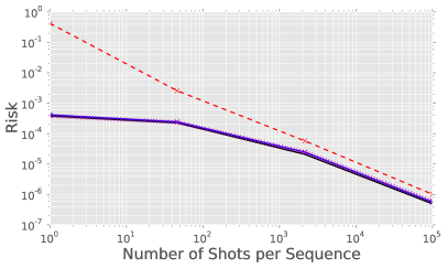
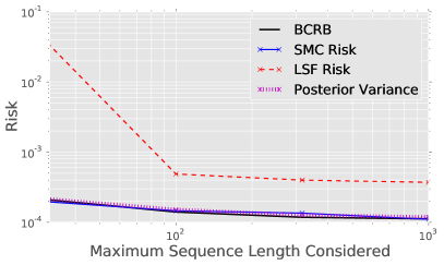
There are essentially two experimental design choices an experimenter can make: the length of the sequence $m$, and the number of repetitions $K$. In the first comparison, we fix the sequence length and vary $K$. In particular, we take all sequence lengths up to 100 for the reference signal and 50 for the interleaved signal. For each such $K$, we plot the mean squared error for the SMC and LSF estimators, along with the posterior variance, which provides an online estimate of the performance of SMC, and the Bayesian Cramer-Rao Bound. The results, shown in Figure 3, demonstrate that SMC can be used to obtain useful estimates of $\tilde{p}$ with a few orders of magnitude less data than is used by least-squares fitting. Moreover, this advantage becomes more pronounced as the number of shots per sequence length approaches one, such that SMC is especially useful in cases where data collection is expensive. We note that this advantage reflects both the performance of SMC itself, and the ability of SMC to take advantage of prior information: for small amounts of data, the least-squares fit estimator chooses estimates far from the initial guess drawn from the prior distribution, while the SMC estimate instead refines the prior. Moreover, SMC can accurately characterize its own performance and can obtain significantly closer accuracy to the ultimate bound given by the BCRB. These advantages are similar to other cases in which SMC shows a large advantage over traditional fitting methods for handling data that is far from deterministic Granade et al. (2012a); Ferrie and Granade (2014).

Figure 4: (Left) Comparison of prior distribution, SMC-approximated posterior, true value and LSF-estimate for $\tilde{p}$ for a single run with $K=1000$ shots at each of $m_{\text{ref}}\in\{1,11,\dots,191\}$ and $m_{C}\in\{2,12,\dots,192\}$. An intentionally inaccurate prior is used, such that the true value is approximately 6.9 standard deviations from the mean of the prior. As shown in Table 1, SMC does well by comparison to LSF, even with the poorly-chosen prior.
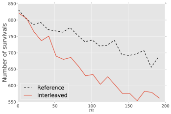
(Right) Data gathered from simulation with physical-model gates.

Figure 5: (Left) Comparison of prior distribution, SMC-approximated posterior, true value and LSF-estimate for $\tilde{p}$ for a single run with $K=100$ shots at each of $m_{\text{ref}}\in\{1,11,\dots,91\}$ and $m_{C}\in\{2,12,\dots,192\}$.
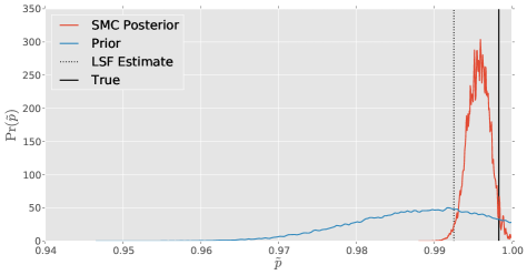
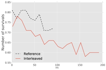
(Right) Data gathered from simulation with physical-model gates.

In Figure 3 (bottom), we show the performance of SMC and LSF when the sequence lengths $m$ vary and the number of shots $K$ per sequence length is fixed, demonstrating that SMC can improve upon LSF especially for very short sequences. Moreover, we see the benefit from increasing the sequence length is minimal compared to repeating experiments at a given sequence length near the optimum length found from the Cramer-Rao bound.

IV Benchmarking with Simulated Gates

Thus far in the analysis, we have used as a simulator the same zeroth-order model as is used to process and interpret the data. To demonstrate the utility of our approach in comparison with traditional LSF-based benchmarking, we now simulate gates according to a cumulant expansion, with physically realistic models. In particular, we use the superconducting model of Puzzuoli et al. (2014) together with optimal control theory Khaneja et al. (2005) to generate a set of gates implementing the target unitaries $\{\mathbbm{1},X,Y,Z,H,P\}$, where $H$ is the Hadamard gate, and where $P=\ket{0}\!\!\bra{0}+\mathrm{i}\ket{1}\!\!\bra{1}$ is the phase gate. We then use the superoperators $\mathchoice{\hat{\vphantom{\rule{1.0pt}{6.14584pt}}\smash{\hat{S}}}}{\hat{\vphantom{\rule{1.0pt}{6.14584pt}}\smash{\hat{S}}}}{\hat{\vphantom{\rule{1.0pt}{6.46875pt}}\smash{\hat{S}}}}{\hat{\vphantom{\rule{1.0pt}{6.92082pt}}\smash{\hat{S}}}}_{U}$ for implementing each target unitary $U$ obtained from a cumulant simulation Kubo (1962); Cappellaro et al. (2006) to sample from the likelihood function (1) .

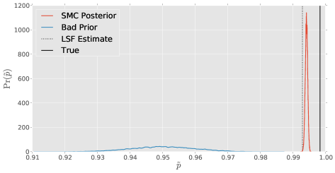
To process these samples, we then use the zeroth-order likelihood function (5) both as a model for sequential Monte Carlo and as a trial function for least-squares fitting. Since the actual implemented gates are known, we can compute the true parameters for comparison. In Table 1, we show the true parameters, the result obtained using SMC, and the result obtained using least-squares fitting. The most important thing to note is that correct parameters are a distance 6.90 $\sigma$ from the prior (meaning the true parameters are outside of the 99.9999998% credible ellipse). This shows that even in the case when the prior information fails to accurately capture the uncertainty in the true model, SMC still does well, providing evidence that our accelerated methods may also be robust, even when used to measure the fidelities of sets of gates with errors that are correlated between distinct gate types, or that include non-trivial unitary components . We show this in more detail in Figure 4, comparing the posterior and prior distributions over $\tilde{p}$ to the true and LSF-estimated values.

Table 1: Results of using SMC and least-squares fitting to estimate the fidelity of $U=X$, simulated using the superconducting qubit gate set. (Left) Bad prior from Figure 4, (right) accurate prior from Figure 5.

	Bad Prior ($40\times 10^{3}$ bits)				Good Prior ($3\times 10^{3}$ bits)
	$\tilde{p}$	$p_{\text{ref}}$	$A_{0}$	$B_{0}$	$\tilde{p}$	$p_{\text{ref}}$	$A_{0}$	$B_{0}$
True	0.9983	0.9957	0.3185	0.5012	0.9983	0.9957	0.3185	0.5012
SMC Estimate	0.9942	0.9971	0.3023	0.5075	0.9957	0.9969	0.2973	0.5010
LSF Estimate	0.9929	0.9974	0.3423	0.4827	0.9925	0.9986	0.5153	0.2782
SMC Error	0.0042	0.0014	0.0161	0.0062	0.0026	0.0011	0.0212	0.0003
LSF Error	0.0054	0.0017	0.0239	0.0185	0.0058	0.0029	0.1968	0.2230

Finally, in Figure 5, we demonstrate the advantage of our method in the presence of physical gates together with a more reasonable prior, and using approximately 10-fold less data than in Figure 4. Taken with other evidence of the robustness of SMC methods Wiebe et al. (2014c); Ferrie and Granade (2014), these results thus show that our method is useful and provides advantages in data collection costs in experimentally-reasonable conditions.

We also note that LSF provides an accurate estimate of $\tilde{p}$ for the simulations with physical gates, but it appears to be at the expense of providing poor estimates for $A$ and $B$. Given that the errors in $\tilde{p}$ and those in $A$ and $B$ are not in general uncorrelated, that LSF often provides such poor estimates of $A$ and $B$ makes the estimates of $\tilde{p}$ derived from LSF difficult to trust.

In this work, we have discussed the fundamental limits of the randomized benchmarking technique that are incurred due to small data sets, and have shown an algorithm that reliably saturates this optimum. In doing so, we have shown that by using sequential Monte Carlo, with a moderate tradeoff in computational costs, one can obtain as much as two orders of magnitude improvement in estimation accuracy, such that data collection requirements are similarly reduced by as much as a hundred-fold. Given the wide and expanding use of randomized benchmarking in experimental practice, this then translates to a significant performance benefit both in benchmarking, and in experimental protocols derived from benchmarking.

Appendix A Sampling Variance and Derivation of Marginalized Likelihood

In this derivation, we will focus on the zeroth-order model of Magesan et al Magesan et al. (2012a), which gives that the average fidelity $F_{g}(m)$ over all sequences of length $m$ is given by

$$F_{g}(m)=A_{0}p^{m}+B_{0}$$ (13)

for constants $A_{0}$ and $B_{0}$ describing the state preparation and measurement (SPAM) errors, and where $1-p$ is the depolarizing strength of $W[\mathbb{E}_{C\sim\mathcal{C}_{n}}\mathchoice{\hat{\vphantom{\rule{1.0pt}{6.14584pt}}\smash{\hat{S}}}}{\hat{\vphantom{\rule{1.0pt}{6.14584pt}}\smash{\hat{S}}}}{\hat{\vphantom{\rule{1.0pt}{6.46875pt}}\smash{\hat{S}}}}{\hat{\vphantom{\rule{1.0pt}{6.92082pt}}\smash{\hat{S}}}}_{C}]$.

We are interested in the single-shot limit, where each measurement consists of first selecting a sequence, then measuring once the survival probability for that sequence. Since this protocol makes no use of the sequence other than its length, we can describe the protocol by marginalizing over the choice of sequence, giving a probability distribution of the form $\Pr(\text{survival}|m)$, where $m$ is a sequence length.

To derive this, we first pick a length $m$, and then consider the choice of sequence $\vec{i}$ out of all length-$m$ sequences to be a random variate. Thus, there exists probabilities

$$p_{m,\vec{i}}:=\Pr(\text{survival}|\vec{i},m)=\mathrm{Tr}(E_{\psi}\mathchoice{\hat{\vphantom{\rule{1.0pt}{6.14584pt}}\smash{\hat{S}}}}{\hat{\vphantom{\rule{1.0pt}{6.14584pt}}\smash{\hat{S}}}}{\hat{\vphantom{\rule{1.0pt}{6.46875pt}}\smash{\hat{S}}}}{\hat{\vphantom{\rule{1.0pt}{6.92082pt}}\smash{\hat{S}}}}_{\vec{i}}[\rho_{\psi}])$$ (14)

for each individual sequence that we could have chosen, such that marginalizing over results in

$$\Pr(\text{survival}|m)=\mathbb{E}_{\vec{i}}[\Pr(\text{survival}|\vec{i},m)].$$ (15)

If each sequence is drawn with uniform probability, then

$$\Pr(\text{survival}|m)=\frac{1}{|\mathcal{C}_{n}|^{m}}\sum_{\vec{i}~{}\text{s.t.}~{}\operatorname{len}\vec{i}=m}p_{m,\vec{i}}.$$ (16)

We recognize this as being the average sequence fidelity $F_{g}(m)$ modeled by Magesan,

$$\Pr(\text{survival}|m)=F_{g}(m)=A_{0}p^{m}+B_{0}.$$ (17)

To interpret $F_{g}(m)$ as a likelihood directly, note that we had to consider the Bernoulli trial (single-shot) limit; had we instead taken $K$ distinct sequences and measured each $N>1$ times, we would have arrived at a quite different quantity

$$\hat{F}_{g}(m)=\sum_{k=1}^{K}\hat{F}(m,\vec{i}_{k}),$$ (18)

where $\hat{F}(m,\vec{i}_{k})$ is the estimate of the sequence fidelity for the particular sequence $\vec{i}_{k}$.

The difference is made clear by considering an example with fixed sequence length $m$, and the variance for a datum $d\sim\Pr(\text{survival}|m)$ (labeling “survival” as 1 and the complementary event as 0),

$$\mathbb{V}_{d}[d|m]=\mathbb{V}_{\vec{i}}[\mathbb{E}_{d}[d|\vec{i},m]]+\mathbb{E}_{\vec{i}}[\mathbb{V}_{d}[d|\vec{i},m]].$$ (19)

The second term corresponds to the mean variance over each fixed sequence $\vec{i}_{m}$, and governs how well we can estimate each $F(m,\vec{i})$ individually. The first term, however, is more interesting, in that it measures the variance over sequences of the per-sequence survival probability $p_{m,\vec{i}}=\mathbb{E}_{d}[d|\vec{i},m]$. By the argument of Wallman and Flammia Wallman and Flammia (2014), this is small when the fidelity being estimated is close to 1; that is, when the gates being benchmarked are very good. For gates that are farther from the ideal Clifford operators, however, or for applications such as tomography via benchmarking Kimmel et al. (2014), this term is not negligible, mandating that many different sequences must be taken for $\hat{F}_{g}(m)$ to be a useful estimate of $F_{g}(m)$.

By demanding that each individual shot be drawn from an independently chosen sequence, our approach avoids this and samples from $d|m$ directly. In this way, we see a similar effect as in Ferrie et al. (2013). In particular, it is not advantageous to concentrate one’s sampling on one point, but to spread samples out and gain experimental variety. Here, the one shot per sequence limit plays the role of the one sample per time-point limit in the earlier discussion.