Enzyme economy and metabolic control

Abstract

The metabolic state of a cell, comprising fluxes, metabolite concentrations and enzyme levels, is shaped by a compromise between metabolic benefit and enzyme cost. This hypothesis and its consequences can be studied by computational models and using a theory of metabolic value. In optimal metabolic states, any increase of an enzyme level must improve the metabolic performance to justify its own cost, so each active enzyme must contribute to the cell’s benefit by producing valuable products. This principle of value production leads to variation rules that relate metabolic fluxes and reaction elasticities to enzyme costs. Metabolic value theory provides a language to describe this. It postulates a balance of local values, which I derive here from concepts of metabolic control theory. Economic state variables, called economic potentials and loads, describe how metabolites, reactions, and enzymes contribute to metabolic performance. Economic potentials describe the indirect value of metabolite production, while economic loads describe the indirect value of metabolite concentrations. These economic variables, and others, are linked by local balance equations. These laws for optimal metabolic states define conditions for metabolic fluxes that hold for a wide range of rate laws. To produce metabolic value, fluxes run from lower to higher economic potentials, must be free of futile cycles, and satisfy a principle of minimal weighted fluxes. Given an economical flux mode, one can systematically construct kinetic models in which all enzymes have positive effects on metabolic performance.

Keywords: Metabolic control theory, cost-benefit analysis, enzyme cost, economic potential, economic balance equation.

1 Introduction

The metabolic fluxes in cells are catalysed and steered by enzyme activities. How should the cell’s enzyme resources be allocated to pathways, to reactions along a pathway, and between the reactions around a metabolite? How will enzyme investments in one place change the incentives for investments elsewhere, given the complex metabolic dynamics and competition for protein resources? At what enzyme cost will a pathway cease to be profitable? And when an enzyme is inhibited, should it be overexpressed (to compensate its lower efficiency) or be shut down together with the rest of the pathway (because the pathway is now inefficient)? An optimal allocation of protein resources implies compromises between metabolic objectives (resulting from fluxes and metabolite concentrations) and enzyme cost (arising, e.g. from a competition for protein resources with other cell processes). Since J. Reichs seminal work on enzyme expression as a cost-benefit problem [1], many optimality principles for optimal fluxes and enzyme profiles have been proposed [2]. In kinetic models, enzyme levels were chosen to maximise metabolic flux at a given total enzyme budget [3] or to minimise enzyme cost [4]. Optimality assumptions can be used to predict how enzyme investments should be distributed along pathways, which pathways should be used, and how these choices depend on the cell’s life conditions. Kinetic models in enzyme-optimal states also serve as starting points for modelling optimal enzyme adaptations [5] and metabolic cycles [6].

While optimal enzyme profiles can be found numerically [7, 8], some questions remain. Can a given flux distribution be realised by an enzyme-optimal state, and can we construct this state and the kinetic model behind it? And are there general principles behind optimal metabolic states or, in other words, economic laws of metabolism? Intuitively, we may expect that the “investome” – the pattern of enzyme costs spent in reactions or pathways – reflects a “usefulness” [9], that is, a benefit these reactions or pathways provide (or in other words, the fitness loss if the reation or pathway did not exist). A relationship between enzyme investments and metabolic control [10] was shown by Klipp and Heinrich [3]. They asked how a pathway flux can be maximised at a given total enzyme amount (and without costs or bounds for metabolite concentrations) and showed that the enzyme levels in the optimal states must be proportional to the scaled flux control coefficients [11, 12]. So in this case, if enzyme levels are seen as investments, scaled flux control can be seen as usefulness! This confirms our intuition: in optimal states, there must be a balance between investments and usefulness, or between cost and benefit – i.e. between the cost of a virtual extra amount of enzyme and the benefit of the resulting flux increase. But do such principles hold more generally? What if different enzymes are differently costly? And what if metabolite costs and other constraints are taken into account? Below I derive economic laws for a wide class of metabolic optimality problems, formulated as balance equations and resembling Kirchhoff’s rules for voltages and currents in electrical circuits. In contrast to Kirchhoff’s rules, these balances do not concern our physical variables (such as metabolite concentrations or fluxes), but economic variables – the costs and benefits, defining the value structure of a metabolic state.

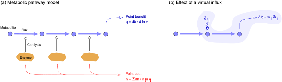
Figure 1: Metabolic cost/benefit problem. (a) metabolic objective and enzyme cost. In the pathway, our running example, metabolic production is scored by a benefit $b(v_{\rm prod})$ while enzyme levels $e_{l}$ are scored by a cost $h({\bf e})$. The cost function may describe opportunity costs in a cell with a limited protein budget, limited space, and limited material and energy. The model may describe a biosynthesis pathway (a series of metabolic reactions) or the cell as a whole (with reactions describing nutrient uptake, metabolism, and macromolecule production, and a flux proportional to the cell growth rate [13]. In each possible state, we can define a benefit $b=\sum_{l}\partial b_{v_{l}}\,v_{l}$ and a cost $h=\sum_{l}h_{e_{l}}\,e_{l}\,e_{l}$ (where $h_{e_{l}}$ may stand, for example, for enzyme molecular mass). (b) Economic potentials. We imagine a virtual influx $\delta r_{i}$ of metabolite $i$, leading to a change of steady-state fluxes and concentrations and to a benefit change $\delta b$. In a linear approximation $\delta b=w_{\rm r_{i}}^{\rm int}\,\delta r_{i}$, the prefactors $w_{\rm r_{i}}^{\rm int}$ are called economic potentials and describe the metabolites’ “use values”. In an optimal state, the potentials increase along the pathway and the equation $v_{l}\,\Delta w_{r_{l}}=h_{e_{l}}\,e_{l}$ must hold in every reaction.

As a running example, we consider a chain of reactions, e.g. a metabolic pathway or a peptide synthetase assembly line consisting of polymerisation reactions (see Figure 1). What are the optimal enzyme levels in this pathway? To specify the problem, we describe the pathway by a kinetic model and define a flux benefit function $b({\bf v})$ that saturates at high fluxes. The enzyme levels $e_{l}$ are scored by a linear cost function $h=\sum_{l}h_{e_{l}}^{\prime}\,e_{l}$ and our aim is to find the enzyme profile that maximises the benefit-cost difference. We can do that by numerical optimisation, with two possible outcomes: if the enzymes are too costly, all reactions will be switched off; otherwise, we obtain an optimal enzyme profile sustaining a positive steady flux. A closer look at this state yields some curious observations: by multiplying the flux $v$ with the benefit derivative ${\rm d}b/{\rm d}v$, we obtain the total enzyme cost. More surprisingly, a similar balance holds for each single reaction. To see this, we define the notion of economic potentials. If we increase the production of metabolite $i$ by an additional “free” influx $\delta r_{i}$, this “gift” will improve the overall benefit, and if we write the increase, in a linear approximation, as $\delta b\approx w_{\rm r_{i}}^{\rm int}\,\delta r_{i}$, the coefficient $w_{\rm r_{i}}^{\rm int}$ is called economic potential. For external metabolites on the pathway boundaries, a different definition of economic potentials is used: the pathway substrate, which does not appear in the benefit function, has a potential of 0, while the pathway product has a potential of ${\rm d}b/{\rm d}v$. If we now compute an optimal state, the economic potentials will always increase along the chain: in every reaction $l$, the difference $\square w_{r_{l}}$ is positive. Moreover, in each reaction the difference $\square w_{r_{l}}$, multiplied by the flux yields exactly the enzyme cost of the reaction! Since all reactions share the same flux, the differences $\square w_{r_{l}}$ and enzyme costs are proportional.

Importantly, all these findings hold for models with any reversible rate laws and any choice of model parameters. For example, if we increase all enzyme cost weights $h_{e_{l}}^{\prime}$ by a constant factor and optimise again, the optimal flux decreases but we obtain the same relationships as before (unless the cost weights become too large; then the enzymes are shut off and the flux will vanish). Even more surprisingly, we can find similar relationships not only for linear pathways, but for metabolic networks of any structure or size, and even for other optimality problems, for example, with regulation arrows or with objectives that penalise high metabolite concentrations. Of course, all these problems could be treated numerically, but since the relations are so general, we may study them as general laws in their own right.

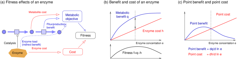
Value/price balance

$\underbrace{\frac{\partial q}{\partial e}}_{\mbox{value}\,y_{\rm e}}=\underbrace{\frac{\partial h}{\partial e}}_{\mbox{price}\,h_{\rm e}}\stackrel{{\scriptstyle!}}{{>}}0$

Benefit/cost balance

$\underbrace{\frac{\partial q}{\partial e}\,e}_{\mbox{point benefit}\,y_{\rm e}^{\centerdot}}=\underbrace{\frac{\partial h}{\partial e}\,e}_{\mbox{point cost}\,h_{\rm e}^{\centerdot}}\stackrel{{\scriptstyle!}}{{>}}0$

Figure 2: Enzyme-optimal states and economic values. (a) Optimal enzyme levels in a kinetic metabolic model. An enzyme (with level $e$) catalyses a reaction with an indirect effect on fluxes $v$ and concentrations $c$ everywhere in the network. A varying enzyme level affects fitness in two ways, via cost and benefit. The metabolic objective $q(e)=b(v^{\rm st}(e))-g(c^{\rm st}(e))$ consists of flux benefit $b(v)$ and metabolite cost $g(c)$, and a cost function $h(e)$ penalises high enzyme levels. The fitness function is defined as the difference ${\mathcal{F}}^{\rm st}(e)=q(e)-h(e)$. (b) metabolic objective $q$ and enzyme cost $h$ as functions of one of the enzyme levels. In the example, benefit and cost depend, respectively, nonlinearly or linearly on enzyme levels. In the optimal point the benefit-cost difference (i.e. fitness), must be maximal, so both curves must have the same slopes. If we call the two slopes “value” (slope of benefit curve) and “price” (slope of cost curve), then value and price must be equal in optimal states. Since all enzyme prices are positive, active enzymes must have a positive (indirect) influence on the metabolic objective. (c) The derivatives of cost and benefit function with respect to logarithmic enzyme levels are called point cost and point benefit. Again, in optimal states point cost and point benefit must be equal.

Metabolic value theory (MVT) [13, 14] defines economic variables that complement the physical variables in a model, describe their fitness values, and are subject to balance equations (Figure 2). Economic values can be defined for a wide range of models by shadow values obtained from optimality problems [14]: to this aim, optimality problems must be written in an “expanded form”, in which all physical laws are formulated as explicit constraints. Each active constraint defines a shadow value. The shadow values arising from mass-balance constraints define values of individual metabolites, called economic potentials [14, 15]. Economic variables for a variety of (kinetic and constraint-based) metabolic models can be defined similarly. Economic values describe the “use value” of network elements, i.e. the effect of small variations of physical variables on fitness as defined in our model. In optimal states, these use values equal to “embodied values” that result from enzyme investments. Formally, the economic laws for metabolic states resemble laws of thermodynamics. Thermodynamic laws relate metabolite concentrations to chemical potentials, thermodynamic forces and flux directions, and must hold in any metabolic system, with any reaction kinetics. Similarly, economic balance equations represent optimal enzyme usage, independent of the details of enzyme kinetics. The laws can also be seen as conservation laws for economic value, describing conserved value flows. In this picture of metabolism, value flows into the system in the form of substrate and enzyme investments, accumulates, and leaves the system in the form of metabolic benefit.

Economic variables describe the value of physical variables, that is, the fitness effects of small variations. The variations need not occur in reality, but are used for mathematical arguments. Optimal states can be characterised by a simple condition: as shown in [14], no legal (that is, constraint-respecting) variation of the state can improve fitness. In the same paper, economic variables were defined through Lagrange multipliers. In a metabolic optimality problem, after expressing all dependencies between model variables by explicit constraints, we obtain Lagrange multipliers associated with these constraints, which can be interpreted as economic variables. Alternatively we can describe constraint-violating variations by perturbation variables: for example, violations of a metabolite’s mass-balance can be described by a virtual influx of the metabolite. In kinetic models, the effects of these perturbations on steady states can be captured by metabolic control or response coefficients, a concept from Metabolic Control Theory (MCT) [11, 16]. The economic variable associated with a constraint can be defined by the response coefficient between a virtual variable (perturbing the constraint) and the system’s objective function. Here I will use this idea for an alternative derivation of metabolic value theory: I consider kinetic metabolic models with enzyme levels as control variables and derive the economic laws from the summation and connectivity theorems of MCT. Economic values are defined by metabolic response coefficients, matching the existing definition by shadow values (see SI section LABEL:sec:ProofsPotentialsAreIdentical). While the previous definition is more general (and also applicable to constraint-based models), the link between metabolic values and metabolic control provides interesting insights and makes a direct connection to Klipp and Heinrich’s results [3].

In this article, we consider kinetic metabolic models whose states are scored by a fitness function, a function of fluxes, metabolite concentrations, and enzyme levels. For steady states with fluxes ${\bf v}^{\rm st}$ and internal concentrations ${\bf c}^{\rm st}$, we obtain the steady-state fitness ${\mathcal{F}}^{\rm st}(\mathbf{e},{\bf x})={\mathcal{F}}({\bf v}^{\rm st}(\mathbf{e},{\bf x}),{\bf c}^{\rm st}(\mathbf{e},{\bf x}),\mathbf{e})$. Optimal states must be enzyme-balanced, that is, the condition $\partial{\mathcal{F}}^{\rm st}/\partial\mathbf{e}=0$ must hold for all active (i.e. expressed) enzymes. As a consequence, each active enzyme must have a positive benefit derivative to balance its cost derivative: in the language of MCT, the response coefficient between enzyme level and benefit function must be positive. Using the theorems of MCT, I show that this implies a principle of local value production: enzymes must produce valuable metabolites from less valuable ones (unless the catalysed flux has a direct benefit). Therefore, fluxes must run from low to high economic potentials, which excludes futile submodes just like thermodynamic constraints would exclude certain flux cycles. Such fluxes are called economical, and only economical fluxes are compatiable with an optimal choice of enzyme levels. Next, I define economic values for metabolite concentrations and metabolic production, derived from the global benefit function. Economic rules and balance equations connect these economic values between metabolites, reactions, and enzymes in the network. Based on these laws, we can construct kinetic models in enzyme-balanced states with predefined fluxes. Such models are useful for studying enzyme adaptation in changing environments [5] or optimal enzyme regulation by effector molecules [17]. The theory holds not only for simple examples – as shown in this paper – but also for large metabolic or non-metabolic systems (e.g. including protein biosynthesis).

2 Kinetic models with cost and benefit terms

To study enzyme-optimal states, here we consider kinetic metabolic models and score their metabolic states by a fitness function (Figure 2 (a)), given by a difference of flux benefit, metabolite cost, and enzyme cost [1, 5, 4] (Figure 2 (b)). In theory, optimal enzyme profiles can be computed numerically, but here we are not interested in in numerical results, but in general laws. To obtain such laws, all network elements (reactions, metabolites, and enzymes) are characterised by economic variables, describing costs and benefits associated with these elements. An economic variable describes how virtual changes in a physical variable affect the overall fitness, either directly or indirectly. While such variables can be defined by Lagrange multipliers, I present here an alternative definition based on methods from MCT: we consider a violation of mass balances by virtual supply fluxes, and study their effects on stationary concentrations and fluxes. Mathematical definitions and proofs can be found in the Supplementary Information (SI). Metabolic value theory introduces new terminology and mathematical symbols: for an overview, see tables LABEL:tab:listofsymbols and LABEL:tab:listofsymbols2 in the SI. MATLAB code is available on github [18]. For more information about metabolic value theory, see www.metabolic-economics.de.

Kinetic metabolic models describe the dynamics of metabolite concentrations $c_{i}$ and chemical reaction rates $v_{l}$. Aside from internal metabolites, there are external metabolites with fixed concentrations $x_{j}$, treated as model parameters. The reaction rates are determined by rate laws $\nu_{l}(\mathbf{e},{\bf c},{\bf x})=e_{l}\,k_{l}({\bf c},{\bf x})$ with enzyme levels $e_{l}$, internal metabolite concentrations $c_{i}$, and external metabolite concentrations $x_{j}$. A flux distribution ${\bf v}$ is called stationary or steady (or a flux profile) if inflows and outflows of internal metabolites are balanced: internal metabolites do not accumulate nor deplete. If all reactions in a flux profile carry non-zero fluxes, the flux profile is called all-active.

To develop a metabolic value theory for kinetic models, we treat enzyme levels in a metabolic pathway or network as control variables that determine a steady state. To describe the effects of enzyme levels $\mathbf{e}$, metabolite concentrations ${\bf c}$, and fluxes ${\bf v}$ on cell fitness, we assume an effective fitness objective ${\mathcal{F}}({\bf v},{\bf c},\mathbf{e})$. Enzymes in cells are costly: even beneficial pathway fluxes may not be profitable if a pathway requires excessive amounts of enzyme [10, 3]. If an enzyme does not contribute to metabolic objective, it should be repressed to save costs. Moreover, the higher a pathway’s enzyme cost, the higher the benefit the pathway needs to provide to balance this cost. To capture these trade-offs, we consider a metabolic pathway or network with variables ${\bf v}$, ${\bf c}$, and ${\bf e}$, and score the possible states by a fitness function

$${\mathcal{F}}({\bf v},{\bf c},\mathbf{e})=b({\bf v})-g({\bf c})-h(\mathbf{e})$$ (1)

comprising a flux benefit $b({\bf v})$, a metabolite cost $g({\bf c})$, and an enzyme cost $h(\mathbf{e})$ [13]. For convenience, we sometimes combine the objective terms and define the metabolic objective $q({\bf v},{\bf c})=b({\bf v})-g({\bf c})$ or the kinetic cost $g^{\rm kin}({\bf c},\mathbf{e})=g({\bf c})+h(\mathbf{e})$. The flux benefit function $b({\bf v})$ may score metabolic production or conversions, cofactor conversion, or biomass production. The cost terms $g({\bf c})$ and $h(\mathbf{e})$ penalise high metabolite or enzyme levels [19, 20]: they describe costly effects (e.g. of occupying space) that arise outside our pathway model [5]. In some cases, the function $g({\bf c})$ may also penalise low metabolite concentrations (e.g. to account for a metabolite’s concentration benefits outside the model pathway).

A fitness function describes what a cell, according to the modeller, strives to maximise to obtain a selection advantage in the growth condition considered. How should we choose it? Fitness functions of the form (1) – a benefit-cost difference – do not follow from deeper biological principles, but are used for mathematical convenience. To obtain fitness functions for pathways, we may start from a cell fitness function $F$ (e.g. the cell growth rate) and define an “optimistic” pathway objective ${\mathcal{F}}({\bf v},{\bf c},\mathbf{e})$ as the maximal possible value of $F$ given our pathway variables ${\bf v},{\bf c},\mathbf{e}$. We can define this function as ${\mathcal{F}}({\bf v},{\bf c},\mathbf{e})=\max_{{\bf z}}F({\bf z}|{\bf v},{\bf c},\mathbf{e})$ where ${\bf z}$ denotes cell variables outside the pathway, to be optimised at given ${\bf v},{\bf c},$ and $\mathbf{e}$ and under the constraints of the cell model. Functions ${\mathcal{F}}({\bf v},{\bf c},\mathbf{e})$ defined in this way may be complicated and possibly not differentiable. For convenience, we replace or approximate them by the simple function Eq. (1) and assume that all three terms are differentiable.

Below we will usually not consider the entire function ${\mathcal{F}}$, but its derivatives (which represent “values”). Typically, the terms $b$ and $g$ in our fitness function (1) score only a small number of model variables: these are the variables with direct fitness effects. Direct (i.e. partial) derivatives of benefit and cost functions, called gains and prices, describe how small variations of fluxes $v_{l}$ or concentrations $c_{i}$ would directly affect the metabolic objective, and how small variations of $e_{l}$ would affect enzyme cost. The flux benefit function $b({\bf v})$ yields the flux gains ${b_{v_{l}}}=\partial b/\partial v_{l}$. For simplicity, we assume flux benefit functions of the form $b^{\star}({\bf v})=b^{\rm dir}({\bf v})+b^{\rm ext}(\mathbf{r}^{\rm ext}({\bf v}))$, with a direct term for fluxes and a term for the external metabolite rates. With ${{\bf b}_{\rm v}^{\rm int}}=\partial b^{\rm dir}/\partial{\bf v}$ and ${\bf b}_{\rm x}=\partial b^{\rm ext}/\partial\mathbf{r}^{\rm ext}$, the flux gain vector reads

$${\bf b}_{\rm v}={{\bf b}_{\rm v}^{\rm int}}+{{\bf N}^{\rm x}}^{\top}\,{\bf b}_{\rm x},$$ (2)

where ${\bf N}^{\rm x}$ is the stoichiometric matrix for external metabolites. The production gains $b_{\rm x_{j}}$ score the production or consumption of external metabolites, while the flux gains ${b_{v_{l}}^{\rm int}}$ score fluxes directly. The splitting of ${\bf b}_{\rm v}$ into flux gains and production gains is not unique and can be chosen by the modeller. The derivatives of the cost terms are called metabolite prices $g_{c_{i}}=\partial g/\partial c_{i}$ and enzyme price $h_{e_{l}}=\partial h/\partial e_{l}$. Enzyme prices are positive, and an enzyme cost function Eq. (3) yields $h_{e_{l}}=h^{\prime}_{l}(\lambda+\lambda^{\rm deg}_{l})\,L_{l}$. If higher metabolite concentrations provide an advantage outside the model pathway, metabolite prices can also be negative. If the metabolic objective depends only on fluxes (flux objective $b({\bf v})$), and not on metabolite levels, the concentration prices vanish. A metabolic objective with a flux gain ${\bf b}_{\rm v}={{\bf N}^{\rm x}}^{\top}{\bf b}_{\rm x}$ and $\mathbf{g}_{\rm c}=0$ (i.e. without flux gains or metabolite prices) is called a production objective. Besides fitness effects, the gains and prices can also reflect the effects of constraints. For example, if a reaction rate must be kept above some minimum value, we can describe this by a flux bound. In this case, our metabolic objective may favour a low flux, but the constraint will prevent this: if the flux hits its lower bound, the “force” that prevents a further decrease is described by a shadow value (Lagrange multiplier) which adds to the flux gain for this reaction (see appendix on “constraints on state variables”). With an an upper flux bound, the effective flux gain is negative, and with inactive bounds it is zero. Similarly, bounds on metabolite concentrations lead to positive prices (for upper bounds) or negative prices (for lower bounds). As a rule of thumb, active lower bounds act like benefits, while active upper bounds act like costs [14].

Enzyme cost functions $h(\mathbf{e})$ for growing microbes have been defined operationally by measuring growth defects caused by an expression of idle proteins. In the cell, these impairments are mediated by complicated processes and compromises (involving enzyme production and maintenance, ribosome production, and limited space due to crowding). Since these effects are not captured by our metabolic model, they are represented by an enzyme cost function $h({\bf e})$. The cost function represents fitness losses due to protein expression that are not included in the metabolic objective function and is typically linear in ${\bf e}$ The derivative $h_{e_{l}}=\partial h/\partial e_{l}$ is called enzyme price, and the derivative ${h_{e_{l}}^{\centerdot}}=\partial h/\partial\ln e_{l}=h_{e_{l}}\,e_{l}$ = is called enzyme investment. With a linear enzyme cost function $h=\sum_{l}h_{l}=\sum_{l}h_{l}^{\prime}\,e_{l}$, the prices $h_{e_{l}}=h_{l}^{\prime}$ are constant and the total enzyme investment is given by the enzyme cost $\sum_{l}{h_{e_{l}}^{\centerdot}}=h$. For a (nonlinear) convex cost function, the prices increase with the enzyme levels, so we obtain a bound $h_{e_{l}}\geq h_{e_{l}}^{\rm min}$ on each price, where $h_{e_{l}}^{\rm min}$ is the price of enzyme $\mbox{\rm e}_{l}$ at zero expression.

3 Conditions for enzyme-optimal states

Our fitness function Eq. (1) implies that the flux benefit should be high and metabolite and enzyme costs should be low. The benefits and costs depend on specific network variables, which gives these variables “direct values” (flux gains for fluxes and metabolite or enzyme prices for metabolites or enzymes). If a flux has a positive gain, it has a positive direct value and the flux should tend to be high. If an enzyme has a positive price, its concentration has a negative direct valueand its concentration should tend to be low. However, we know that our state variables cannot be chosen independently: in steady states, they are coupled. If one of them changes, the others will change as well. therefore, a variable has also indirect fitness effects through all other variables. For instance, if an enzyme (while being costly) catalyses a reaction that contributes to the flux benefit, the enzyme becomes beneficial itself. To find the right enzyme level, we need to balance this benefit with the cost. The principle same applies for all physical variables in the system: each variable needs to be chosen such that its costs and benefits are in balance (which includes indirect costs and benefits, and shadow values due to constraints). To get an impression of the resulting states, we now consider fitness maximisation in the entire coupled system.

To define enzyme-optimal states in metabolis,, we score the enzyme profile by a fitness function

$${\mathcal{F}}(\mathbf{e},{\bf x}) = q(\mathbf{e},{\bf x})-h(\mathbf{e}).$$ (4)

with a metabolic objective $q(\mathbf{e},{\bf x})=b({\bf v}^{\rm st}(\mathbf{e},{\bf x}))-g({\bf c}^{\rm st}(\mathbf{e},{\bf x}))$ and an enzyme cost $h(\mathbf{e})$. The vectors ${\bf v}^{\rm st}$ and ${\bf c}^{\rm st}$ describe steady-state fluxes and concentrations. We now search for enzyme levels $e_{l}$ that maximise fitness. Variants of this optimality problem – models with multi-functional enzymes or non-enzymatic reactions, other constraints, or multi-objective optimisation – are discussed in appendix A.3 and B.

What can we know about the pattern of enzyme investments and fluxes in enzyme-optimal states? To see this, we consider a local optimum of ${\mathcal{F}}(\mathbf{e})$ and have a look at the optimality conditions. In an interior optimum state, in which all enzymes are active, the difference $t_{e_{l}}=\partial{\mathcal{F}}/\partial e_{l}=y_{e_{l}}-h_{e_{l}}$ is called total enzyme value (or enzyme stress). In an optimal state, it must vanish, $\partial{\mathcal{F}}/\partial e_{l}=0$, which implies an equality (see Figure 2 b),

$$y_{e_{l}}=h_{e_{l}}$$ (5)

between enzyme value $y_{e_{l}}=\frac{\partial q({\bf v}^{\rm st}({\bf e}),{\bf c}^{\rm st}({\bf e}))}{\partial e_{l}}$ and enzyme price $h_{e_{l}}=\frac{\partial h({\bf e})}{\partial e_{l}}$. If the equality holds, then not only enzyme prices, but also enzyme values must be positive, i.e. all enzymes must have a positive influcence on the metabolic objective. If a metabolic state satisfies the “value-price balance” Eq. (5) in all active enzymatic reactions, it is called enzyme-balanced, and all models in enzyme-optimal states must in fact be enzyme-balanced. If the equality (5) does not hold, this indicates a non-optimal state, and the enzyme stresses describe “incentives” to change and improve the enzyme levels $e_{l}$.

What about optimal states in which variables hit bounds? All enzyme levels are bounded from below ($e_{l}\geq 0$ because they cannot be negative), and for inactive enzymes ($e_{l}=0$) the bound leads to a negative shadow price that balances out the enzyme price. Likewise, active upper bounds on enzyme levels lead to shadow prices that act like cost terms and add to the regular enzyme price. In a pathway model, enzyme levels are not bounded from above but penalised by a cost, and we may think of this cost as an opportunity cost in a larger cell model with a fixed protein budgte, where an enzyme increase in a pathway leaves less protein for other pathways, thus reducing their benefit. If enzymes in the optimal state remain inactive, the enzyme profile is a boundary optimum and we obtain optimality conditions $e_{l}>0$ and $v_{l}\neq 0$ for active enzymes and $e_{l}=0$ and $v_{l}=0$ for inactive ones. An active reactions must satisfy Eq. (5), while in inactive reactions the enzyme levels vanish and the optimality condition is an inequality $\partial{\mathcal{F}}/\partial e_{l}<0$: expressing this enzyme would decrease the fitness, which means that the enzyme price $h_{e_{l}}$ exceeds the value $y_{e_{l}}$ (see SI Figure LABEL:fig:costbenefitcurves2).

Enzymes are costly. For each reaction, the enzyme investment per reaction flux defines “flux burden” $a_{v_{l}}=\frac{\delta h}{\delta v_{l}}=\frac{\delta h}{\delta e_{l}}\,\frac{\delta e_{l}}{\delta v_{l}}$, an effective overhead price of the flux. Here we assume that enzymes are reaction-specific and that each reaction is catalysed by a single enzyme. Under this “unique enzyme assumption”, we obtain a diagonal enzyme elasticity matrix with elements ${E^{\rm v_{l}}_{\rm e_{l}}}=\frac{\partial v_{l}}{\partial e_{l}}=\frac{v_{l}}{e_{l}}=k_{l}$. This matrix is invertible unless $k_{l}=0$ (e.g. if reactions are in thermodynamic equilibrium). With the help of this matrix and the enzyme price $\frac{\partial h_{l}}{\partial e_{l}}=h_{e_{l}}$, flux burdens can be computed as follows. Considering a variation of an enzyme level and its direct effect on reaction rates, the flux burden is defined $a_{v_{l}}=\frac{h_{e_{l}}}{{E^{\rm v_{l}}_{\rm e_{l}}}}=\frac{h_{e_{l}}}{k_{l}}=\frac{h_{e_{l}}\,e_{l}}{v_{l}}$. If the flux cost $a^{\rm enz}$ in an FBA model is given by an enzymatic flux cost function (from an underlying kinetic model) [23], the flux burden vector ${\bf a}_{\rm v}$ (in the kinetic model) is equal to the gradient $\nabla_{{\bf v}}a^{\rm enz}({\bf v})$. Using these definitions, our balance Eq. (5) for enzyme values and prices can now be converted into a similar equation for flux values and prices: by multiplying with the “enzyme slowness” $e_{v}/v_{l}$ (i.e. dividing by the catalytic rate), we obtain the flux value balance

$$\underbrace{y_{e_{l}}\,\frac{e_{l}}{v_{l}}}_{w_{v_{l}}}=\underbrace{h_{e_{l}}\,\frac{e_{l}}{v_{l}}}_{a_{v_{l}}},$$ (7)

between flux value and flux burden in each reaction.

4 Variation rules

The optimality conditions (5) can be used to check the results of a numerical optimisation, but it also provides more general insights: it leads to general economic laws for enzyme-optimal states, valid for any rate laws and cost function which will be explored below. Below, starting from Eq. (5), I derive the basic laws of metabolic value theory and introduce the notion of economic potentials. For simplicity, we usually assume that flux benefit $b({\bf v})$ and metabolite cost $g({\bf c})$ are linear functions, so flux gains and metabolite prices are constant and known. A simple production objective depends only on a single production rate; in such cases, this single product has a production gain, while all other production gains, flux gains, and metabolite prices vanish. But this does not mean that other variables (in particular enzyme levels across the network) are not important. How can we infer the role of each enzyme, i.e. the profile of enzyme values across the network? And how are the two types of variables – direct gains and prices, and indirect enzyme values – related? If we perturb an enzyme, we may predict the effect on value production by following causal chains in the network. If we start from where production benefit is actually realised, then to see how this is supported by enzymes elsewhere we need to follow causal chains in reverse, from effect to cause: step by step, value is “acquired” from variable to variable in backwards direction. How is this “propagation of economic value” shaped by network structure and kinetics? Remember, we are not interested in anecdotical numerical results, but in general laws. Thus, we will ask: what can we learn from cost-benefit balance Eq. (5) about optimal metabolic states? Can we learn something about possible flux profiles even without knowing the rate laws? At first sight, this may be surprising: the sensitivities $y_{e_{l}}$, which must be matched by the enzyme prices, depend on enzyme kinetics. However, we can still learn about metabolic fluxes by using metabolic control theory (MCT).

Metabolic Control theory describes how local parameter perturbations affect metabolic states. The effect of parameter perturbations on steady-state fluxes and concentrations are quantified by sensitivities called metabolic response coefficients. The metabolic response coefficient $R^{z}_{e_{l}}=\partial z/\partial e_{l}$, between an enzyme level $e_{l}$ and a state variable $z$, can be written as a product $R^{z}_{e_{l}}=C^{z}_{v_{l}}\,E^{v_{l}}_{e_{l}}$ where the enzyme elasticity $E^{v_{l}}_{e_{l}}$ describes how an enzyme perturbation perturbs the reaction rate (at constant metabolite levels), and the control coefficient $C^{z}_{v_{l}}$ describes how this rate perturbation changes our steady-state variable $z$. To see how MCT can help us characterise enzyme-optila fluxes, consider an enzyme variation $\delta{\bf e}$, leading to a perturbed reaction rate. The metabolic control coefficients describe the global effects of this perturbation (see Figure LABEL:fig:costbenefitcurves1). By using these coefficients, we can write the enzyme value as

$$y_{e_{l}} = \frac{\partial q}{\partial e_{l}}=\sum_{j}{b_{v_{j}}}\,R^{\rm V}_{jl}-\sum_{i}g_{c_{i}}\,R^{\rm C}_{il}=\left(\sum_{j}{b_{v_{j}}}\,C^{\rm V}_{jl}-\sum_{i}g_{c_{i}}\,C^{\rm S}_{il}\right)\,\frac{v_{l}}{e_{l}}.$$ (8)

The formula describes a chain of effects: an enzyme’s direct effect on a reaction rate (elasticity $E^{v_{l}}_{e_{l}}=v_{l}/e_{l}$), the indirect influence of this rate on the stationary fluxes and concentrations (metabolic control coefficients $C^{\rm V}_{lr}=\frac{\partial v^{\rm st}_{l}}{\partial e_{r}}\frac{v_{r}}{e_{r}}$ and $C^{\rm S}_{ir}=\frac{\partial c^{\rm st}_{i}}{\partial e_{r}}\frac{v_{r}}{e_{r}}$), and their direct effects on the metabolic objective (flux gains ${b_{v_{l}}}$ and metabolite prices $g_{c_{i}}$). The difficult terms in Eq. (8) are the metabolic control coefficients $C^{\rm V}_{jl}$ and $C^{\rm S}_{il}$, which are nonlocal and state-dependent (i.e. to know them, we need to know the solution to the optimality problem). However, Eqs (5) and (8) yield a general rule: the balance condition (5) requires that any expressed enzyme must have a positive value $y_{e_{l}}$ and therefore a non-zero catalytic rate $v_{l}/e_{l}$. This means: if an enzyme is completely inhibited or if it catalyses an equilibrium reaction (and thus $k_{l}=v_{l}/e_{l}=0$), the enzyme must not be expressed (“principle of dispensable enzyme” [13]).

To do this, let us formulate our optimality conditions in the language of metabolic control theory. By definition, an enzyme value $y_{e_{l}}=\partial q/\partial e_{l}$ is the metabolic response coefficient between enzyme level $e_{l}$ and metabolic objective $q$, and the flux value $w_{v_{l}}=y_{e_{l}}/{E^{\rm v_{l}}_{\rm e_{l}}}=y_{e_{l}}\frac{e_{l}}{v_{l}}$ is the corresponding control coefficient (see SI LABEL:sec:proofenzymebenefitmetabolitevalue for details). With control matrices $\mathbf{C}^{\rm V}$ and $\mathbf{C}^{\rm S}$, the flux values can be written as (compare Fig. 4)

$${\bf w}_{\rm v}^{\top}={\bf b}_{\rm v}^{\top}\,\mathbf{C}^{\rm V}-{\bf g}_{\rm c}^{\top}\mathbf{C}^{\rm S}.$$ (9)

Obviously, the flux values $w_{v_{l}}$ in Eq. (9) cannot be inferred from network structure alone: like other control coefficients, they depend on kinetics and on the (optimal) metabolic state. So again, what can we learn about metabolic values from network structure alone?

If the flux values $w_{v_{l}}$ are control coefficients, they must satisfy summation and connectivity theorems [2]. By combining Eqs (5) and (8) and applying these theorems, we obtain the variation rules (Proposition LABEL:th:theorem1 in SI)

$${\bf b}_{\rm v}\cdot{\boldsymbol{\kappa}} = \frac{{\bf h}_{\rm e}\,\circ{\bf e}}{{\bf v}}\cdot{\boldsymbol{\kappa}}$$ (10)

$$\mathbf{g}_{\rm c}\cdot\boldsymbol{\ell} = \mathbf{E}_{\rm c}^{\top}\,\frac{{\bf h}_{\rm e}\circ{\bf e}}{{\bf v}}\cdot\boldsymbol{\ell},$$ (11)

which must hold for all vectors ${\boldsymbol{\kappa}}$ and $\boldsymbol{\ell}$ with the following properties. The vector ${\boldsymbol{\kappa}}$ in the flux variation rule is a column (or linear combination of columns) of the null space matrix ${\bf K}$, i.e. a stationary flux distribution (satisfying ${\bf N}^{\rm int}\,{\boldsymbol{\kappa}}=0$). The vector $\boldsymbol{\ell}$ in the concentration variation rule is a column (or linear combination of columns) of the link matrix ${\bf L}$, i.e. a profile of internal metabolic concentration variations that leave the conserved moieties unchanged (satisfying $\mathbf{G}\,\boldsymbol{\ell}=0$). In short, both vectors must describe valid, i.e. constraint-respecting variations. The dot $\cdot$ denotes the scalar product, while multiplication $\circ$ and division of vectors apply componentwise, and $\mathbf{E}_{\rm c}$ is the elasticitiy matrix in our metabolic state. The variation rules relate flux gains ${b_{v_{l}}}$ and concentration prices $g_{c_{i}}$ to enzyme investments ${\bf h}_{\rm e}\circ{\bf e}$ and inverse fluxes. With the flux burdens $a_{v_{l}}=h_{e_{l}}\,e_{l}/v_{l}$, we can write them as

$$({\bf b}_{\rm v}-{\bf a}_{\rm v})\cdot{\boldsymbol{\kappa}} = 0$$ (12)

$$(\mathbf{g}_{\rm c}-\mathbf{E}_{\rm c}^{\top}\,{\bf a}_{\rm v})\cdot\boldsymbol{\ell} = 0\;,$$ (13)

which must hold, again, for all valid vectors ${\boldsymbol{\kappa}}\in\mbox{Span}({\bf K})$ and $\boldsymbol{\ell}\in\mbox{Span}({\bf L})$. If we replace these vectors by valid infinitesimal variations, we obtain the variation rules in differential form

$$({\bf b}_{\rm v}-{\bf a}_{\rm v})\cdot{\delta_{\parallel}}{\bf v} = 0$$ (14)

$$(\mathbf{g}_{\rm c}-\mathbf{E}_{\rm c}^{\top}\,{\bf a}_{\rm v})\cdot{\delta_{\parallel}}{\bf c} = 0.$$ (15)

The flux variation rule (14) must hold for all valid flux variations ${\delta_{\parallel}}{\bf v}$ (i.e. stationary variations satisfying ${\bf N}^{\rm int}\,{\delta_{\parallel}}{\bf v}=0$) and the metabolite variation rule (15) must hold for all valid concentration variations ${\delta_{\parallel}}{\bf c}$ (i.e. moiety-conserving variations, satisfying $\mathbf{G}\,{\delta_{\parallel}}{\bf c}=0$). The two rules refer to models with active, enzyme-catalysed reactions and without metabolite dilution. For models with inactive or non-enzymatic reactions, or for models with metabolite dilution, the formulae must be modified (see SI LABEL:sec:proofSummationConnectivity).

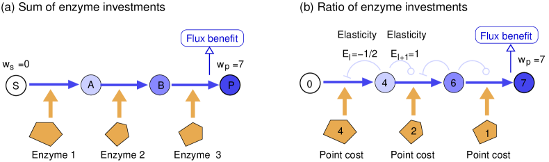
Flux variation rule $\sum_{l}{b_{v_{l}}}\,v_{l}=\sum_{l}{h_{e_{l}}^{\centerdot}}$:
Total flux point benefit = Total enzyme investment

Metabolite variation rule $\frac{E_{l}}{E_{l+1}}=\frac{{{h_{e}^{\centerdot}}}_{l+1}}{{{h_{e}^{\centerdot}}}_{l}}$:
Enzyme investment ratio = Inverse elasticity ratio

Figure 3: Enzyme investments predicted by the variation rules. (a) Metabolic pathway with production objective $b({\bf v})=w_{\rm P}\,v_{\rm P}$, where $w_{\rm P}$ and $v_{\rm P}$ are, respectively, the economic potential and the production rate of product P. Aoccrding to the flux variation rule (14), in optimal states the sum of enzyme investments $\sum_{l}h_{e_{l}}\,e_{l}$ must be equal to the sum of flux point benefits $\sum_{l}\square w_{\rm r_{l}}^{\rm int}\,v_{l}=w_{p}\,r_{p}$. The investments accumulate along the chain, and by summing all enzyme investments upstream of a given metabolite, we obtain the investment embodied in this metabolite. The “embodied” investments in the product is equal to the total benefit. By dividing a metabolite’s embodied investment by its production rate (i.e. the pathway flux), we obtain the metabolite’s economic potential (shades of blue). As expected, the economic potentials rise along the flux. If the initial substrate has an economic potential $w_{\rm S}>0$, this corresponds to a substrate investment, which further increases the economic potentials of all following metabolites. (b) The reaction elasticities determine the ratios of optimal enzyme investments. The metabolite variation rule (15) states that enzyme investments for adjacent (producing and consuming) reactions are inversely proportional to the elasticities ${E^{\rm v_{l}}_{{\rm c}_{i}}}=\partial v_{l}/\partial c_{i}$. In the example (with flux $v=1$, substrate elasticities 1, product elasticities -1/2, and total benefit 7), we obtain enzyme investments ${h_{e_{l}}^{\centerdot}}=(4,2,1)$. They decrease along the pathway, confirming the result from [3].

The variation rules (14) and (15) for enzyme-optimal states determine optimal enzyme investments. Figure 3 shows an example, a linear pathway with given flux gains ${\bf b}_{\rm v}$, concentration prices $\mathbf{g}_{\rm c}$, and flux distribution ${\bf v}$. The flux variation rule (14) shows that the scalar products ${\bf b}_{\rm v}\cdot{\boldsymbol{\kappa}}$ (“point benefit”) and ${\bf a}_{\rm v}\cdot{\boldsymbol{\kappa}}$ (”point cost”) must be equal for any stationary flux variation ${\boldsymbol{\kappa}}$ (given by ). If we use the flux profile ${\bf v}$ itself as a flux variation, the resulting equality ${\bf v}\cdot\,{\bf b}_{\rm v}={\bf v}\cdot({\bf h}_{\rm e}\circ{\bf e}/{\bf v})=\sum_{l}h_{e_{l}}\,e_{l}$ shows that the sum of enzyme investments is determined by ${\bf v}$ and ${\bf b}_{\rm v}$. How will this investment be distributed along a pathway? In the metabolite variation rule (15), the ratio of enzyme investments around a metabolite depends on the reaction elasticities for this metabolite. Taken together, in a linear pathway with known elasticities, the variation rules determine all enzyme investments completely. With a linear enzyme cost function, enzyme investments are proportional to enzyme abundance and follow from proteomics data. But the variation rules can also be used in reverse: given the enzyme investments, flux gains, and flux directions, we may predict the metabolic fluxes (proof in SI LABEL:sec:UniquenessProof). Two simple examples (a linear pathway and a branch point model) and an algorithm for larger networks are given in SI LABEL:sec:fluxesfromenzymecosts.

The flux variation rule (14) relates fluxes and flux gains to enzyme cost. If flux gains ${b_{v_{l}}}$ and enzyme investments $h_{e_{l}}\,e_{l}$ are known, we obtain linear constraints on the inverse fluxes. In a linear pathway (or a network with only one flux mode) this constraint can be used to scale our flux distribution. More generally, the rule tells us – given a change in some of the variables – how other variables must be adapted for the cell to remain in an optimal state. For example, a higher flux (at a constant flux gain ${b_{v_{l}}}$) leads to a higher flux benefit and justifies a higher enzyme investment $h_{e_{l}}\,e_{l}$. In contrast, with lower flux gains ${b_{v_{l}}}$ (and constant investments $h_{e_{l}}\,e_{l}$), the flux must increase (this requiring a higher catalytic rate). And when enzyme prices $h_{e_{l}}$ increase and the enzyme levels $e_{l}$ are fixed, the fluxes must increase to maintain an optimal state. These links between enzyme investments and fluxes are not due to kinetics alone, but to our optimality postulate. By using kinetic relationships between enzyme levels and fluxes, we can further limit the possible optimal states. And even if ${{\bf h}_{e}^{\centerdot}}$ and $\mathbf{E}_{\rm c}$ are unknown, the simple fact that the ${{\bf h}_{e}^{\centerdot}}$ must be positive puts constraints on the fluxes. We will later come back to this point.

5 Economic variables

The variation rules characterise optimal states by referring to valid state variations, for instance stationary flux variations that may concern the entire network. To consider such variations, we need a global picture of the system considered. But can optimal states also be characterised locally, by laws that describes a single enzyme and its catalysed reaction, a single reaction and the surrounding metabolites, or a single metabolite and the surrounding reactions? This seems unlikely because a local perturbation will have effects elsewhere in the network: it will have indirect effects on fitness through its action on other variables. We saw that optimality conditions (e.g. Eq. (5)) depend on such indirect effects. Hence, a local description may not suffice to understand optimal states: instead, we need to consider network-wide, indirect effects described by indirect economic values.

In metabolic value theory, all metabolites, reactions, and enzymes carry economic values. Two other important types of economic values, called economic potentials and economic loads, are assigned to metabolites. An economic potential describes how a metabolite rate contributes to the metabolic objective (i.e. the (indirect) value of metabolite production). To define it, we consider a virtual extra supply of the metabolite and ask how this would change the overall metabolic objective by changing the system state. The economic loads, in contrast, describe the (indirect) value of metabolite concentrations: they quantify how a virtual concentration change would contribute to the benefit by changing the system state.

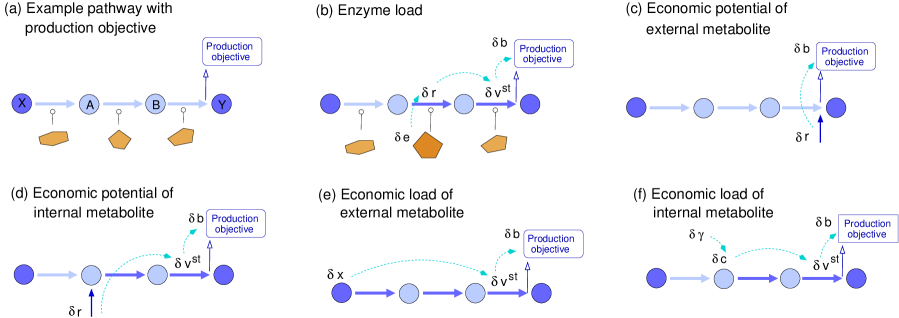
Figure 4: Economic values in a linear pathway. (a) Example pathway with production objective (production of metabolite Y). (b) Enzyme values $y_{\rm e}$ describe how enzyme level variations $\delta e$ change the metabolic objective in steady state. The indirect effect is mediated through a chain of effects $\delta{\bf e}\rightarrow\delta{\bf v}^{\rm st}\rightarrow\delta b$. Accordingly, the (indirect) enzyme value is obtained from a chain of derivatives (ratios of differentials $y_{\rm e}=\frac{\delta q}{\delta e}=\frac{\delta q}{\delta v}\frac{\delta v}{\delta k}\frac{\delta k}{\delta e}$). The sensitivity $C^{\rm J}=\frac{\delta v}{\delta k}$ (a flux control coefficient) describes the effect of a local rate perturbation ($\delta k$) on the stationary flux ($\delta v$).Other economic variables are defined similarly. (c) Economic potentials $w_{\rm r}^{\rm int}=\delta q/\delta{r}^{\rm int,vrt}$ of external metabolites describe the effect of a virtual production change $\delta{r}^{\rm int,vrt}$. (d) Economic potentials $w_{\rm r}^{\rm ext}=\delta q/\delta{r}^{\rm int,vrt}$ of internal metabolites describe the effects of virtual supply fluxes $\delta{r}^{\rm int,vrt}$. (e) Economic loads $y^{\rm x}=\delta q/\delta x$ of an external metabolite $x$ describes the effects of virtual concentration changes $\delta x$. (f) Economic loads $y^{\rm c}=\delta q/\delta{c^{\rm vrt}}$ of internal metabolites describe the effects of virtual concentration changes $\delta{c^{\rm vrt}}$.

Let us first consider the economic potentials (see Figures 4 (c) and (d)). Each metabolite carries an economic potential, which assigns an indirect value to the metabolite’s production rate and which describes how a steady extra supply of the metabolite would change the overall fitness. If it increases the fitness, the economic potential $w_{r_{i}}$ (fitness change $\delta{\mathcal{F}}$ per extra flux $\delta r_{i}$) is positive. Generally, an economic potential consists of two terms: a direct value (or “production gain”) and an indirect value (or “production load”). For external metabolites $j$, the indirect value vanishes and the potential is given by the direct value $w_{r_{j}}^{\rm ext}=b_{\rm x_{j}}$. For internal metabolites $i$, the direct term vanishes (because of the zero net rate) and only the indirect value remains. This indirect value can be defined by control coefficients. To define economic potentials mathematically, we imagine a virtual supply flux ${r}^{\rm int,vrt}_{i}$ that adds to the production of the metabolite. To inspect its effects on the steady state and on fitness, we write the metabolic objective as a function $q(\mathbf{e},{\bf x},{\mathbf{r}}^{\rm int,vrt})$ of enzyme levels $e_{l}$, external levels $x_{j}$, and virtual supply fluxes ${r}^{\rm int,vrt}_{i}$ and define the indirect production value of a metabolite $i$ by the response coefficient $y_{r_{i}}=\frac{\partial q}{\partial{r}^{\rm int,vrt}_{i}}$. We now set the economic potential to $w_{\rm r_{i}}^{\rm int}=y_{r_{i}}$. In models with moiety conservation (e.g. if the sum [ATP]+[ADP] remains unchanged in all reactions), additional supply fluxes (e.g. a supply of ATP) may violate moiety conservation (e.g. the total concentration of ATP and ADP) and cause a non-steady state. To avoid this, in the definition of economic potentials [27] we describe supply fluxes by supply flux vectors (describing simultaneous inflows and outflows of different metabolites), which must allow for a steady state. To construct such vectors, we first consider a supply flux vector ${\mathbf{r}}{{}^{\rm ind,vrt}}$ for independent metabolites only, which can be chosen without constraints, and then define the supply flux vector ${\mathbf{r}}^{\rm int,vrt}={\bf L}\,{\mathbf{r}}{{}^{\rm ind,vrt}}$. The economic potentials of dependent metabolites are defined to be to zero by convention.

We saw that economic potentials are economic values associated with metabolite rates. Similarly, economic loads are the economic values values associated with concentrations. A metabolite concentration can influence the metabolic objective in two ways: directly, by as described by its price, and indirectly via its effects on the steady state (see Figures 4 (e) and (f)). We see describe this by considering virtual concentration changes. A change $\delta c_{i}$ of metabolite $i$ changes the metabolic objective, and the concentration value $w_{\rm c_{i}}$ describes this effect. A concentration value $w_{\rm c_{i}}=y_{c_{i}}-g_{c_{i}}$ consists of a direct value (the negative metabolite price $-g_{c_{i}}$) and an indirect value $y_{c_{i}}$, called economic load: the load describes how a virtual concentration variation of our metabolite would affect the metabolic objective indirectly, via changes of the network-wide metabolic state. External metabolite concentrations $x$, as predefined variables, usually have no direct value and their concentration values are directly given by their load $y_{x_{j}}=\frac{\partial q}{\partial x_{j}}$. Internal metabolite concentrations, in contrast, can have a price, and the relationship between price and load depends on the existence of conserved moieties. If metabolites in a cell are diluted, their economic potentials contribute their “effective economic load” (see Section 7). Finally, also other model variables, such as growth rate, compartment volumes or temperature, can be associated with economic loads. In summary, a metabolite load denotes an indirect concentration value acquired through the metabolite’s concentrations effect on adjacent reactions (and therefore, on the entire metabolic state); for external metabolites, the total concentration value is directly given by the load, i.e. by the response coefficient on the metabolic objective, and there is no concentration price. For internal metabolites, the total concentration value vanishes, and is given by the difference of load and concentration price.

6 Local economic rules

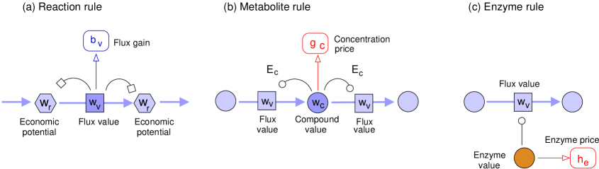
${\bf w}_{\rm v}={{\bf b}_{\rm v}^{\rm int}}+\underbrace{{{\bf N}^{\rm tot}}^{\top}\,{\bf w}_{\rm r}}_{\square{\bf w}_{\rm r}}$

${\bf w}_{\rm c}=-\mathbf{g}_{\rm c}+\underbrace{\mathbf{E}_{\rm c}^{\top}\,{\bf w}_{\rm v}}_{{\bf y}_{\rm c}}$

${\bf t}_{\rm e}=-{\bf h}_{\rm e}+\underbrace{\mathbf{E}_{\rm e}^{-1}{\bf w}_{\rm v}}_{{\bf y}_{\rm e}}$

Figure 5: Economic rules describe the economic values of neighbouring network elements. (a) Reaction rule. The flux value of a reaction consists of a direct flux value (the flux gain ${b_{\rm v}^{\rm int}}$) and an indirect flux value (given by the economic potential difference $\square w^{\rm c}$). (b) Metabolite rule. A concentration value $w_{\rm c_{i}}$ consists of a direct value (the negative concentration price $-g_{c}$) and an indirect value (the economic load $y_{c_{i}}$, acquired from the neighbouring flux values of adjacent reactions). Other variables that impact reaction rates, like temperature, are associated with economic variables satisfying similar economic rules (not shown). (c) Enzyme rule. The total value (or “economic stress”) of an enzyme is given by the enzyme’s use value (or “load”) $y_{\rm e}=w_{\rm v}\frac{v}{u}$ minus the enzyme price $h_{\rm e}$. Assuming that each reaction is specificylly catalysed by one enzyme, we can set $\mathbf{E}_{\rm e}^{-1}=\mbox{\rm Dg}(k)^{-1}=\mbox{\rm Dg}(\mathbf{e})\mbox{\rm Dg}({\bf v})^{-1}=\mbox{\rm Dg}({\boldsymbol{\tau}})$. The ratio $\tau_{l}=e_{l}/v_{l}=1/k_{l}$ is also called “enzyme slowness”. All these economic rules also hold for non-optimal states. In optimal states, the total values of enzymes must vanish, so enzyme use values and enzyme prices must be equal.

If a models variable influences the metabolic objective indirectly, this variable has a “use value” (quantified by an economic variable). Computing this value may require knowledge about the entire system. Formulae such as Eq. (8) for individual enzymes, the control coefficients refer to state variations in the entire network (caused by a local variation, but extending over large parts of the system). How can we describe metabolic variations and values locally, without considering the entire system? To do so, we may consider “invalid” variations of a single reaction or a single metabolite (that violate mass balances or moiety conservation and require compensation by virtual perturbation variables). Describing these variables by metabolic value theory, we obtain local economic rules that relate economic variables between neighbour elements in the network. Each rule refers to a type of variable and relates its economic value to the economic values of neighbouring variables in the network (see Figure 5).

1. Reaction rule A flux value $w_{v_{l}}$ describes the overall influence of a reaction flux $v_{l}$ on the metabolic objective. The reaction rule (see Fig. 5 (a))

   $$w_{v_{l}}=\underbrace{{b_{v_{l}}^{\rm int}}}_{w_{v_{l}}^{\rm dir}}+\underbrace{\square w_{r_{l}}}_{y_{v_{l}}},$$ (16)

   describes it as a sum of two terms: a direct flux value (given by the flux gain ${b_{v_{l}}^{\rm int}}$, plus a shadow value for fluxes that hit a constraint), and an indirect flux value $y_{v_{l}}=\square w_{r_{l}}=\sum_{i}n_{il}\,w_{r_{i}}$ acquired from the reactants and given by the difference of economic potentials along the reaction (proof and explanations see SI LABEL:sec:SIderivationReactionRule and LABEL:sec:proofenzymebenefitmetabolitevalue). Thus, the economic value of a flux – a global systemic property! – can formally be attributed to the local conversion of metabolites of different values.

2. Metabolite rule A concentration value $w_{\rm c_{i}}$ describes the influence of a metabolite concentration on the metabolic objective. According to the metabolite rule (Fig. 5 (b))

   $$w_{\rm c_{i}}=\underbrace{-g_{c_{i}}}_{w_{\rm c_{i}}^{\rm dir}}+\underbrace{\sum_{l}{E^{\rm v_{l}}_{{\rm c}_{i}}}\,w_{v_{l}}}_{y_{c_{i}}},$$ (17)

   it consists of an indirect and a direct value. The direct value is given by the negative concentration price $-g_{c_{i}}$ (plus a shadow value for metabolites that hit concentration bounds). The indirect value is called economic load and is given by $y_{c_{i}}=w_{\rm c_{i}}+g_{c_{i}}$. The metabolite rule implies that economic loads are given by $y_{c_{i}}=\sum_{l}{E^{\rm v_{l}}_{{\rm c}_{i}}}\,w_{v_{l}}$ (Figure 5 (b) and proof in SI LABEL:sec:loadproof). What can we learn from this rule? Typically, external metabolites are assigned a vanishing price $g_{c_{i}}=0$. In models with dilution, the sum in Eq. (17) contains an extra term $-\lambda\,w_{\rm r_{i}}^{\rm int}$ (see section 7), which describes a value loss due to dilution. By incorporating the dilution term into the price $w_{\rm c_{i}}$, we obtain the effective price $w_{\rm c_{i}}^{\rm eff}=w_{\rm c_{i}}+\lambda\,w_{\rm r_{i}}^{\rm int}$. In models without moiety conservation, the metabolites’ concentration values vanish ($w_{\rm c_{i}}=0$), and so metabolite load and metabolite price are balanced ($y_{c_{i}}=g_{c_{i}}$). In models with moiety conservation, we obtain the weaker condition ${\bf L}^{\top}\,{\bf w}_{\rm c}=0$, entailing a balance equation ${\bf L}^{\top}\,{\bf y}_{\rm c}={\bf L}^{\top}\,\mathbf{g}_{\rm c}$.

3. Enzyme rule The total value (or “stress”) $t_{e_{l}}=\partial{\mathcal{F}}/\partial e_{l}$ of an enzyme is described by the enzyme rule (Fig. 5 (c))

   $$t_{e_{l}}=\underbrace{-h_{e_{l}}}_{w_{e}^{\rm dir}}+\underbrace{E^{v_{l}}_{e_{l}}\;w_{v_{l}}}_{y_{e_{l}}}.$$ (18)

   The total enzyme value results from a direct price (the enzyme price $h_{e_{l}}$) and an indirect value $y_{e_{l}}$ (or “enzyme load”), which represents the enzyme’s influence on the metabolic objective. The indirect value is acquired from the flux value $w_{v_{l}}$ of the catalysed reaction. If a reaction is catalysed by a (specific) enzyme, the enzyme elasticity is given by ${E^{\rm v_{l}}_{\rm e_{l}}}=e_{l}/v_{l}$ and the enzyme load reads ${\bf y}={\bf e}/{\bf v}\circ{\bf w}_{\rm v}=\mbox{\rm Dg}(\mathbf{e})\,\mbox{\rm Dg}({\bf v})^{-1}\,{\bf w}_{\rm v}$. In optimal states, the total enzyme value must vanish (because enzyme levels are control variables), unless the enzyme level hits a bound (the bound $e\geq 0$ for positivity, $e\leq 0$ for some specified upper bound, or $sum_{l}e_{l}=e_{\rm tot}$). In such constrained optimal states, the total enzyme value must be balanced by a shadow value. In non-optimal states, the total value $t_{e_{l}}$ can be positive or negative (implying, respectively, that the cell should increase or decrease the enzyme level to reach an optimal state).

Taken together, the economic rules are the basic laws for economic potentials in metabolic networks, similar to Kirchhoff’s rules for voltages and currents in electric circuits.

All economic rules share the same simple form: an economic value consists of a direct and an indirect part, where the direct value is a gain or price (i.e. a direct fitness derivative, plus a possible shadow values for upper and lower bounds), while the indirect value (representing fitness effects via steady-state changes) is “acquired” from the neighbour network elements).

In each of the rules, the direct term represents a gain or price, which may include a shadow gain or shadow price due to a bound on the physical variable. For example, consider an enzyme level that hits the lower bound $e=0$. In this case, a shadow value $h_{e_{l}}^{\rm bnd}$ is subtracted from $h_{e_{l}}$ in Eq. (18) [14]. If we include this term (as a direct term) into the enzyme price, we obtain the effective enzyme price $h_{e_{l}}^{\rm eff}=h_{e_{l}}+h_{e_{l}}^{\rm bnd}$, and in an optimal state the effective price will vanish. Effective flux gains $b_{v_{l}}^{\rm eff}={b_{v_{l}}^{\rm int}}+{b_{v_{l}}^{\rm int}}^{\rm bnd}$ and metabolite prices $g_{c_{i}}^{\rm eff}=g_{c_{i}}+g_{c_{i}}^{\rm bnd}$ are defined similarly. For simplicity, theis will be be explicitly mentioned below.

The direct economic values (flux gains $b_{\rm v}$, metabolite prices $g_{c}$, and enzyme prices $h_{\rm e}$) arise from fitness derivatives and bounds on single variables. While each enzyme (and possibly each metabolite) has a direct price, we typically assume that only a few fluxes carry direct values. For example, with biomass production as the metabolic objective, only the biomass-producing reaction has a direct flux benefit. But all reactions, metabolites, and enzymes may contribute indirectly to this benefit and therefore carry a use value.

The economic rules for the economic values of neighbour elements show how variables “acquire” indirect use values from “child variables”. The direct values arise from the fitness function (and bounds), and the indirect values arise from “propagating” these direct values across the network. If the direct values in a network are known, can we infer all other values from them? Assuming we know the connection coefficients, this is fact possible: given the reaction elasticities, flux gains, and metabolite prices in an enzyme-balanced state, the economic potentials and loads can be directly determined. For generality, we consider models with moiety conservation and dilution, see SI sections LABEL:sec:proofenzymebenefitmetabolitevalue and LABEL:sec:SIproofMCAwithDilution. From the economic rules for such models, we obtain a yield a formula for the internal economic potentials

$${\bf w}_{\rm r}^{\rm int} = ({\bf L}\,{\mathbf{M}_{\lambda}}^{-1}\,{{\bf L}^{+}})^{\top}\,\underbrace{\mathbf{g}_{\rm c}-\mathbf{E}_{\rm c}^{\top}\,{\bf b}_{\rm v}}_{\mathbf{g}^{\star}_{\rm c}}.$$ (19)

The proximal concentration price $\mathbf{g}^{\star}_{\rm c}$ consists of the direct price and an indirect price acquired from adjacent reaction gains. In the equation, $\mathbf{M}_{\lambda}={\bf N}^{\rm ind}\,\mathbf{E}_{\rm c}\,{\bf L}-\lambda\,\mathbf{I}$ is the Jacobian matrix (for models with dilution), and the projection matrix ${{\bf L}^{+}}$ maps concentrations from internal metabolites to independent internal metabolites (proof and example in SI LABEL:sec:SIProofsolveForEcoPot). Equation (19) can be visualised geometrically: if the flux gains are described by a sparse vector in a high-dimensional space, vector of economic potentials is a “projection” of this vector (which concerns only one or a few reactions) onto the entire network. Similar projections exist in MCT: If a reaction rate is perturbed (e.g. by an enzyme inhibition), the perturbation can be described by a sparse, non-stationary flux vector $\delta{\bf v}$. The resulting flux change (a stationary flux vector $\delta{\bf v}^{\rm st}$) is obtained by left-multiplying this vector with ${\bf C}^{\rm v}$, so ${\bf C}^{\rm v}$ acts as a projector onto the subspace of stationary flux distributions. This analogy between the two theories is not by chance: in one case, the projection reflects the response of a mechanistic system (mediated through chains of causal effects), in the other case it reflects economic requirements (mediated through chains of incentives, in the opposite direction). For details, see SI LABEL:sec:SIvirtualVariations.

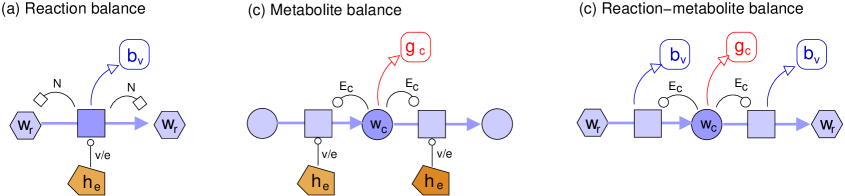
$\underbrace{\square w_{r_{l}}+{b_{v_{l}}^{\rm int}}}_{w_{v_{l}}}=\underbrace{h_{e_{l}}\,e_{l}/v_{l}}_{a_{v_{l}}}$

$y_{c_{i}}=\sum_{l}{E^{\rm v_{l}}_{{\rm c}_{i}}}\,\underbrace{h_{e_{l}}\,e_{l}/v_{l}}_{a_{v_{l}}}$

$y_{c_{i}}=\sum_{l}\underbrace{(\square w_{r_{l}}+{b_{v_{l}}^{\rm int}})}_{w_{v_{l}}}\,{E^{\rm v_{l}}_{{\rm c}_{i}}}$

$(\square w_{r_{l}}+{b_{v_{l}}^{\rm int}})\,v_{l}=h_{e_{l}}\,e_{l}$

$y_{c_{i}}\,c_{i}=\sum_{l}\hat{E}^{\rm v_{l}}_{{\rm c}_{i}}\,h_{e_{l}}\,e_{l}$

$y_{c_{i}}\,c_{i}=\sum_{l}(\square w_{r_{l}}+{b_{v_{l}}^{\rm int}})\,v_{l}\hat{E}^{\rm v_{l}}_{{\rm c}_{i}}$

Figure 6: Economic balance equations. Each equation can be written in “value form” (top) or “value production form” (bottom). (a) The reaction balance equation states that flux values and flux burdens of a reaction must be equal. It follows from the optimality condition for enzyme levels, $t_{e_{l}}=y_{e_{l}}-h_{e_{l}}=0$ (see Figure (5)). variables denote the economic potential difference $\square w_{r_{l}}$, flux $v_{l}$, direct flux gain ${b_{v_{l}}^{\rm int}}$, price $h_{e_{l}}$, and flux burden $a_{v_{l}}=h_{e_{l}}e_{l}/v_{l}$. In reactions with a direct flux gain $b_{v}=0$, the equation requires $\Delta w_{\rm r_{l}}^{\rm int}$ and $v_{l}$ to have the same signs and the economic potentials must increase along the flux. Multiplying the equation with the flux $v_{l}$ yields the value production form (bottom). (b) The metabolite balance equation (with economic load $y_{c_{i}}=g_{c_{i}}$; flux cost weight $a_{v_{l}}={h_{e_{l}}^{\centerdot}}/v_{l}$; scaled elasticity $\hat{E}^{\rm v_{l}}_{{\rm c}_{i}}$) relates a metabolite’s economic load $y_{c_{i}}$ to the enzyme investments around the metabolite. In models without moiety conservation, optimality requires that load $y_{c_{i}}$ and metabolite price $g_{c_{i}}$ must be equal. In models with moiety conservation, we can augment $\mathbf{g}_{\rm c}$ to ${\mathbf{g}_{\rm c}}^{\rm eff}=\mathbf{g}_{\rm c}+{\bf w}_{\rm c}=\mathbf{g}_{\rm c}+\mathbf{G}^{\top}\,{\bf w}_{\rm cm}$. (c) The reaction-metabolite balance relates the economic load of a metabolite (shaded) to the flux values of neighbour reactions (and thus to economic potentials).

7 Economic balance equations

The economic rules (16), (17), and (18) explain a variable’s economic value by a direct value and by an indirect value acquired from the variable’s child variables (i.e. variables directly influenced by it). The rules hold for all metabolic states, including non-optimal states and non-enzymatic reactions. But we are particularly interested in enzyme investments in optimal states. If enzyme levels are choice variables (and do not hit a constraint), their total value in optimal states must vanish. By setting the enzyme stresses $t_{e_{l}}=0$ in Eq. (18), we obtain economic rules for optimal states. Then, by combining the rules in pairs, we obtain balance equations that relate enzyme investments to economic potentials, loads, and costs in neighbouring reactions, metabolites, and enzymes (see Figure 6).

1. Reaction balance By setting Eq. (18) to zero (assuming expressed enzymes in an enzyme-optimal state) and inserting Eq. (16), we obtain the reaction balance in “enzyme value form”

   $$(\square w_{r_{l}}+{b_{v_{l}}^{\rm int}})\,{E^{\rm v_{l}}_{\rm e_{l}}}=h_{e_{l}}$$ (20)

   between flux value and enzyme price, which must hold for all active enzymatic reactions. Assuming a one-to-one relation between reactions and enzymes, the enzyme elasticity ${E^{\rm v_{l}}_{\rm e_{l}}}$ is given by the catalytic rate $k_{l}=v_{l}/e_{l}$. Dividing Eq. (20) by $k_{l}$ and noting that $h_{e_{l}}/k_{l}=a_{v_{l}}$, we obtain the equation in “flux value form”

   $$\square w_{r_{l}}+{b_{v_{l}}^{\rm int}}=a_{v_{l}}$$ (21)

   with the flux burden $a_{v_{l}}=\frac{h_{e_{l}}}{k_{l}}=\frac{h_{e_{l}}\,e_{l}}{v_{l}}$ defined as above. Eq. (21) shows that the economic potential (or “use value”) $w_{r_{i}}$ of a metabolite is equal to an “embodied value”: in reactions with out flux gains (i.e. ${b_{v_{l}}^{\rm int}}=0$) the potential increases from substrate to product because of the flux burden $a_{v_{l}}$, reflecting the enzyme investment in the reaction. Therefore, along a pathway flux the metabolite values will tend to increase and will embody all upstream enzyme (and external substrate) investments. The step from Eq. (20) to Eq. (21) assumes that the $e_{l}$ are actually enzyme levels (which appear as prefactors) in the rate laws, that every reaction is enzyme-catalysed, and that enzymes are reaction-specific. This “unique enzyme assumption” guarantees that the enzyme elasticity matrix $\mathbf{E}_{\rm e}=\mbox{\rm Dg}({\bf v}/{\bf e})$ is diagonal. If we further exclude zero enzyme elasticities, the matrix will be invertible. Otherwise (e.g. in the case of non-specific enzymes other control variables $u_{l}$ such as temperature or membrane potentials), the elasticity matrix will not be invertible and Eq. (31) must be replaced by modified formulae (see appendix B).

2. Metabolite balance Our second balance equation relates a metabolite’s economic load to the flux burdens in the adjacent reactions (reactions that a metabolite influences kinetically as a reactant, catalyst, or regulator). For internal metabolites (with concentations $c_{i}$ and loads $y_{c_{i}}$) and external metabolites (with concentrations $x_{j}$ and loads $y_{x_{j}}$), the equalities read (proof see SI LABEL:sec:proofinvestmentbalance)

   $$y_{c_{i}}=\sum_{l}a_{v_{l}}\,{E^{\rm v_{l}}_{{\rm c}_{i}}},\qquad y_{x_{j}}=\sum_{l}a_{v_{l}}\,{E^{\rm v_{l}}_{{\rm x_{j}}}}.$$ (22)

   To derive the metabolite balance Eq. (22), we assume that all reactions are enzyme-catalysed. A variants of this equation can include non-enzymatic reactions (see Eq. (LABEL:eq:qloadinternal3) in appendix). If reaction rates depend on variables other than metabolite concentrations (e.g. temperature), these variables also have economic loads satisfying similar balance equations.

3. Reaction-metabolite balance The value of metabolite production and of metabolite concentrations are described, respectively, by economic potentials and loads. How are these values related? In growing cells, with dilution fluxes $v_{i}^{\rm dil}=\lambda c_{i}$, metabolite concentrations and fluxes are coupled by ${\bf c}=\frac{1}{\lambda}{\bf N}^{\rm int}\,{\bf v}$, on top of their coupling through rate laws. Thus, concentration change affects the neighbouring reaction rates, which further affect metabolite net rates and eventually (in a steady growth state) their concentrations. How is all this reflected in value structure? The loads ${\bf y}_{\rm c_{i}}$ of internal metabolites are given by ${\bf y}_{\rm c}=\mathbf{g}_{\rm c}-\mathbf{G}^{\top}\,{\bf w}_{\rm cm}$. Eq. (17) relates a metabolic load to the flux values $w_{v_{l}}$ in adjacent reactions (with rates directly affected by the metabolite). By inserting the reaction balance (21), we obtain the reaction-metabolite balance

   $$y_{c_{i}}=\sum_{l}\underbrace{(\square w_{r_{l}}+{b_{v_{l}}^{\rm int}})}_{w_{v_{l}}}\,{E^{\rm v_{l}}_{{\rm c}_{i}}}.$$ (23)

   between the load of metabolite $i$, the flux gains ${b_{v_{l}}^{\rm int}}$ and economic potentials $w_{r_{i}}$ in the adjacent reactions and the elasticities ${E^{\rm v_{l}}_{{\rm c}_{i}}}$ between them. Similar equations exist for external metabolites and other variables that influence reaction rates (e.g. temperature).

As mentioned before, the direct value terms can contain shadow values arising from bounds on the physical variables. Interestingly, reaction and metabolite balance resemble each other. The reason is that enzymes can be seen as external metabolites: their concentrations are constant, and they influence reaction rates kinetically. Accordingly, the reaction balance (20) resembles a metabolite balance (22) with an enzyme instead of an external metabolite (with elasticity ${E^{\rm v_{l}}_{{\rm x_{j}}}}=\frac{v_{l}}{e_{l}}$ and a load $y_{x_{j}}=h_{e_{l}}$ given by the enzyme price).

The economic laws shown above hold for models without dilution. In growing cells, metabolite dilution can be described conveniently by “degradation fluxes” $v^{\rm dil}_{i}=\lambda\,c_{i}$ with the growth rate $\lambda$ as a rate constant. For steady states, we obtain a mass-balance equation $0={\bf N}^{\rm int}\,{\bf v}-\lambda\,{\bf c}$ that couples concentrations directly to fluxes. This coupling has consequences for metabolic economics. If cell growth is the objective, the dilution rate of compounds, including metabolites and macromolecules, can be treated as the fitness objective. The resulting balance equations (with growth rate as a control variable and objective) are discussed in [14]. Here we consider a different problem: a metabolic pathway with a given production objective, in which metabolites are diluted at a given rate $\lambda$. Dilution puts a burden on metabolism, which reshapes the optimal enzyme investments.

For example, consider a linear pathway with a production objective (scoring the last reaction flux). In growing cells, higher internal metabolite concentrations will increase the dilution fluxes and the waste of enzyme investment embodied in the metabolites. To keep the metabolite concentrations low while maintaining the desired flux, enzyme investments must be rearranged: upstream enzyme levels should decrease and downstream enzyme levels increase.

To model this, we can describe dilution by “dilution reactions” with velocity $v_{i}^{\rm dil}=\lambda\,c_{i}$, elasticity $E^{\rm v^{\rm dil}_{i}}_{\rm c_{i}}=\lambda$, and flux values $w_{v}=\square w_{\rm r}^{\rm int}=-w_{r}$ (assuming there is no flux gain and no “product” of the dilution reaction). For each metabolite, this reaction leads to an extra term $-\lambda\,w_{\rm r_{i}}^{\rm int}$ on the right of the reaction-metabolite balance. We can see the term $-\lambda\,w_{\rm r_{i}}^{\rm int}$ as a concentration price, describing an incentive to keep $c_{i}$ low: by including it into $g_{c_{i}}$, we obtain the effective concentration prices $g_{c_{i}}^{\prime}=g_{c_{i}}+\lambda\,w_{\rm r_{i}}^{\rm int}$, which are higher than the “real” prices $g_{c_{i}}$ (or less negative, for metabolites with a negative price). Alternatively, we can bring the term $-\lambda\,w_{\rm r_{i}}^{\rm int}$ to the left and define the effective economic load $y_{c_{i}}^{\rm eff}=y_{c_{i}}+\lambda\,w_{\rm r_{i}}^{\rm int}$. In the metabolite balance equation, the extra term $\lambda\,w_{v_{l}}$ on the left needs to be balanced by the sum on the right. To increase this sum, investments are shifted from producing to consuming reactions. This confirms our expectations: dilution favours enzyme investments that keep metabolite concentrations low.

8 Balance equations for point cost and benefit

Economic values (such as gains, prices, potentials, or loads) are derivatives between fitness and physical variables. If fitness is measured in units of Darwin (Dw), a placeholder for the respective fitness unit used in a model, we obtain the unit Dw/mM for economic loads (a fitness derivative for concentrations) and Dw/(mM/s) for economic potentials (a fitness derivates for metabolite rates), and possibly other units. To make all economic values comparable, we can define fitness derivatives with respect to logarithmic variables, ${\mathcal{F}}_{x}^{\centerdot}=\frac{\partial{\mathcal{F}}}{\partial\ln x}=\frac{\partial{\mathcal{F}}}{\partial x}x={\mathcal{F}}_{x}\,x$ (see Figure 2): all these “point” derivatives have units of Dw, the unit of the fitness function itself! Note that the point value of a variable is just the normal economic value, multiplied with the variable’s own numerical value. By writing economic laws with these new derivatives, we obtain the laws in the so-called “value production form” form (as opposed to our previous “value form”). Now different processes can be directly compared: for example, if a reaction substrate (characterised by a net consumption rate) and and enzyme (characterised by a concentration) contribute to the overall benefit, their benefit contributions (“point benefits”) are directly comparable.

Let us see an example. To rewrite the optimality condition Eq. (5) in value production form, we simply multiply it by $e_{l}$ (see Figure 2c). The resulting equation

$$\underbrace{y_{e_{l}}\,e_{l}}_{y_{{e_{l}}}^{\centerdot}}=\underbrace{h_{e_{l}}\,e_{l}}_{{h_{e_{l}}^{\centerdot}}}$$ (24)

relates the enzyme point benefit (or “value production”) $y_{{e_{l}}}^{\centerdot}=\frac{\partial q}{\partial\ln e_{l}}=y_{e_{l}}\,e_{l}$ to the point cost (or enzyme investment) ${h_{e_{l}}^{\centerdot}}=\frac{\partial h}{\partial\ln e_{l}}=h_{e_{l}}\,e_{l}$. Except for the dots, the equation looks just like Eq. (5). An active enzyme represents a positive investment: in an optimal state, it must also have a positive point benefit! By rewriting the left side $y_{e_{l}}\,e_{l}=w_{v_{l}}\,v_{l}$, we can express it as a rate of value production. The principle of local value production, a condition for enzyme-optimal states, can be used as a constraint in flux balance analysis. Using flux values, it can also be written as $w_{v_{l}}\,v_{l}>0$. Finally, by dividing Eq. (24) by the flux $v_{l}$ and defining the flux burden $a_{v_{l}}=\frac{h_{e_{l}}\,e_{l}}{v_{l}}$, we reobtain our balance equation (7).

Let us now consider economic variables in value production form more generally. if we describe direct values not by usual derivatives, but by logarithmic derivatives, we obtain flux point benefits ${b_{v_{l}}}^{\centerdot}=\partial b/\partial\ln v_{l}={b_{v_{l}}}\,v_{l}$, metabolite point costs $g_{c_{i}}^{\centerdot}=\partial g/\partial\ln c_{i}=g_{c_{i}}\,c_{i}$, and enzyme point costs (“enzyme investments”) ${h_{e_{l}}^{\centerdot}}=\partial h/\partial\ln e_{l}=h_{e_{l}}\,e_{l}$. A flux point benefit ${{\bf b}_{\rm v}}^{\centerdot}={\bf b}_{\rm v}\cdot{\bf v}$ determines whether a flux profile is beneficial (${{\bf b}_{\rm v}}^{\centerdot}>0$), futile (${{\bf b}_{\rm v}}^{\centerdot}=0$, i.e. satisfying ${{\bf N}^{\rm ben}}\,{\bf v}={{\bf b}_{\rm v}^{\top}\choose{\bf N}^{\rm int}}\,{\bf v}=0$), or wasteful (${{\bf b}_{\rm v}}^{\centerdot}<0$). Futile or wasteful flux profiles are called non-beneficial. We further introduce the flux point cost (or “flux investment”) $a_{v_{l}}^{\centerdot}=a_{v_{l}}\,v_{l}$, which her, in kinetic models, is equal to $h_{e_{l}}/k_{l}$. In short, for our present models, we obtain $a_{v_{l}}^{\centerdot}={h_{e_{l}}^{\centerdot}}$, i.e. flux and enzyme investments are equal. “Point” versions of indirect values are defined similarly. Like in the example above, all economic laws can be written in value production form by by multiplying each economic variable with the corresponding physical variable (i.e. replacing economic values by “point” values).

1. Reaction balance The reaction balance in value production form relates value production to enzyme investment. In an optimal state, all active reactions must satisfy the value-price balance (20). By multiplying this balance with the enzyme level $e_{l}$, we obtain the reaction balance in value production form

   $$\underbrace{(\square w_{r_{l}}+{b_{v_{l}}^{\rm int}})\,v_{l}}_{y_{e_{l}}=w_{v_{l}}^{\centerdot}}=\underbrace{h_{e_{l}}\,e_{l}}_{{h_{e_{l}}^{\centerdot}}}.$$ (25)

   It states that the flux point benefit $w_{v_{l}}^{\centerdot}=(\square w_{r_{l}}+{b_{v_{l}}^{\rm int}})\,v_{l}$ (the local value production) must be equal to the enzyme investment ${h_{e_{l}}^{\centerdot}}=h_{e_{l}}\,e_{l}$, and therefore to the flux point cost $a_{v_{l}}^{\centerdot}=a_{v_{l}}\,v_{l}$. Like the flux variation rule (14), the reaction balance (25) holds for any types of rate laws. Here are some practical consequences. Since active enzymes have positive costs, flux value $w_{v_{l}}=\square w_{r_{l}}+{b_{v_{l}}^{\rm int}}$ and flux $v_{l}$ must have equal signs, so in reactions without direct flux gain (${b_{v_{l}}^{\rm int}}=0$), the flux must lead from lower to higher economic potentials. In reactions with direct flux gains (${b_{v_{l}}^{\rm int}}\neq 0$), fluxes may run in the orther direction if the flux gain is sufficiently high. Turning this logic around, we can ask: given a flux profile ${\bf v}$, can there be internal economic potentials $w_{\rm r_{i}}^{\rm int}$ and positive enzyme investments ${h_{e_{l}}^{\centerdot}}$ that satisfy the reaction balance? For economical flux profiles ${\bf v}$, the answer is yes (Propositions LABEL:th:theoremtestmode and LABEL:th:theoremfutile). For uneconomical flux profiles – e.g. flux profiles with futile cycles – no consistent potentials ${\bf w}_{\rm r}^{\rm int}$ can be found. This closely resembles the role of chemical potentials in thermodynamic flux analysis [28].

2. Metabolite balance By multiplying the metabolite balance Eq. (22) with the concentration $c_{i}$, we obtain the metabolite balance in point form

   $$\underbrace{w_{\rm c_{i}}\,c_{i}}_{y_{c_{i}}^{\centerdot}}=\sum_{l}\underbrace{h_{e_{l}}e_{l}}_{{h_{e_{l}}^{\centerdot}}}\,\hat{E}^{\rm v_{l}}_{{\rm c}_{i}}$$ (26)

   with the scaled elasticities $\hat{E}^{\rm v_{l}}_{{\rm c}_{i}}=\frac{c_{i}}{v_{l}}{E^{\rm v_{l}}_{{\rm c}_{i}}}$. The equation relates a metabolite’s point load $y_{c_{i}}^{\centerdot}$ to the enzyme investments ${h_{e_{l}}^{\centerdot}}$ around the metabolite. On the right, we find a linear combination of enzyme investments with scaled elasticities $\hat{E}^{\rm v_{l}}_{{\rm c}_{i}}$ as (positive or negative) prefactors. As we already know, in models without conserved moieties, $y_{c_{i}}^{\centerdot}$ is equal to the concentration price $g_{c_{i}}^{\centerdot}$. If a metabolite load vanishes (e.g. an internal metabolite without direct fitness effects that is not involved in moiety conservation), the sum on the right must vanish, so for each metabolite, we obtain a linear constraint on the enzyme levels. By defining ratios of enzyme levels, these constraints shape the proteome.

   What else can we learn from Eq. (26)? Consider the pathway in Figure 3. If the fitness function contains no metabolite costs (and therefore, $\mathbf{g}_{\rm c}=0$), enzyme investments and reaction elasticities around a metabolite are inversely proportional: ${h_{e_{l}}^{\centerdot}}/h_{e_{l+1}}^{\centerdot}=|E^{v_{l}}_{c_{l}}/E^{v_{l+1}}_{c_{l}}|$. We already know this from the metabolite variation rule (see Figure 3). Typically, reaction substrates have larger scaled elasticities than reaction products. Hence, if “production” and “consumption” refer to flux directions (and not just to nominal reaction orientations) [29], producing reactions have higher flux burdens than consuming reactions, so flux burdens tend to decrease along the flux. If our metabolite has a price $g_{c_{i}}>0$, this price appears in the balance equation and implies a positive load $y_{c_{i}}>0$: in this case, consuming reactions must have higher elasticity-weighted enzyme investments than producing reactions: this configuration makes intuitive sense because it keeps the metabolite concentration low. What about extracellular compounds? Compounds with a positive influence on the metabolic objective (and with a positive concentration) have positive point loads, their import deserves an investment. In contrast, metabolites with a vanishing concentration or vanishing (or negative) load are not profitable for the cell: their transporters provide no benefit and should not be expressed.

3. Reaction-metabolite balance By multiplying Eq. (23) by $c_{i}$, we obtain the reaction-metabolite balance in value production form

   $$\underbrace{y_{c_{i}}\,c_{i}}_{y_{c_{i}}^{\centerdot}}=\sum_{l}\underbrace{(\square w_{r_{l}}+{b_{v_{l}}^{\rm int}})\,v_{l}}_{w_{v_{l}}^{\centerdot}}\,\hat{E}^{\rm v_{l}}_{{\rm c}_{i}},$$ (27)

   with the point load $y_{c_{i}}^{\centerdot}$ and flux point value $w_{v_{l}}^{\centerdot}$. We can briefly write it as $y_{c_{i}}^{\centerdot}=\sum_{l}w_{v_{l}}^{\centerdot}\,\hat{E}^{\rm v_{l}}_{{\rm c}_{i}}$.

When describing the value structure of metabolism, can we also describe non-optimal states? The economic balance equations assume optimal enzyme levels. In reality, cells do not behave optimally, at least not precisely, and certainly not for our simple optimality criteria. Even without expression noise or leaky transcription, cells would always be maladapted after perturbations such as gene knock-downs. Apparent non-optimality may arise from side objectives or from preemptive expression, and enzyme levels may not be optimal at all. However, it may be practical to describe non-optimal states by using our optimality formalism. In fact, metabolic value theory defines economic variables and rules for any metabolic state, not just optimal states. The only difference is that, in non-optimal states, there are economic imbalances (or “stresses”) $t_{e_{l}}^{\centerdot}=\frac{\partial{\mathcal{F}}}{\partial e_{l}}=y_{e_{l}}-h_{e_{l}}$ that describes a mismatch between the values and prices of enzymes. Since all stresses (of expressed enzymes) must vanish in optimal states, they were not considered in the economic balance equations (meant to describe optimal states). To describe non-optimal states, we can include them as extra terms, yielding the reaction imbalance (see SI LABEL:sec:violationsnonenzymatic)

$$(\square w_{r_{l}}+{b_{v_{l}}^{\rm int}})\,v_{l} = (h_{e_{l}}+t_{e_{l}})\,e_{l}.$$ (28)

The stress $t_{e_{l}}$ implies an imbalance between enzyme cost and benefit: a positive stress (indicating that an enzyme level is too low for an optimal state) yields the economic imbalance

$$(\square w_{r_{l}}+{b_{v_{l}}^{\rm int}})\,v_{l} > h_{e_{l}}\,e_{l}.$$ (29)

In this case (i.e. a flux stress with the same sign as the flux), the enzyme’s point benefit exceeds the point cost, and the cell would be able to improve its fitness by increasing the enzyme level. Of course, with a negative stress (i.e. an enzyme level higher than required for an optimal state), the inequality changes its sign, and the enzyme level should be decreased. If a non-optimal state is due to a constraint (e.g. a bound on a flux to model an enzyme knock-down), the constraint will lead to a shadow value, and this shadow value can be included into the flux gain in brackets. Non-zero stresses indicate a non-optimal state, and how the cell can improve this state by changing the enzyme levels – that is, they hint at selection pressures. Imagine that a cell cannot perform some useful reaction because it has no enzyme for it. To quantify the incentive for having this enzyme, we could start from the current metabolic state and include the reaction into the network, but assume that the system (with an enzyme price $h_{e_{l}}$) is not expressed. The flux value of the new, inactive reaction is given by

$$\underbrace{\square w_{r_{l}}+{b_{v_{l}}^{\rm int}}}_{w_{v_{l}}} = (h_{e_{l}}+t_{e_{l}})\,\underbrace{e_{l}/v_{l}}_{k_{l}}=a_{v_{l}}+t_{v_{l}}.$$ (30)

A flux stress $t_{v_{l}}=t_{e_{l}}/k_{l}=w_{v_{l}}-a_{v_{l}}$ describes an imbalance between flux value $w_{v_{l}}$ and flux burden $a_{v_{l}}$. A positive stress (or more precisely, a stress with the same sign as the desired reaction rate) indicates that evolving the enzyme would be profitable for the cell.

Enzyme investments (point costs) and benefit contributions (point benefits) have the same measurement units and satisfy conservation relations, which suggests that they may be interconvertible. We can see them as different forms of the same “substance”, just like heat and work are different forms of a “substance” called energy. More specifically, the value production equation can be seen as a conservation law for “value flows” (see Fig. 7): in the “value flow picture”, enzyme investments are values that flow into the system, are become benefit contributions, and eventually reach reactions and metabolites in which benefit is realised, and flow from there into the benefit function. The conversion between Enzyme investments and benefit contributions happens in every single reaction: coming from substrate and enzyme, value flows into the reaction and towards the product and into the direct flux benefit. As shown in Fig. 7 (c), by rewriting enzyme values as $y_{e_{l}}=w_{v_{l}}\,\frac{e_{l}}{v_{l}}$, the cost-benefit balance Eq. (24) can be written as

$$\underbrace{w_{v_{l}}\,v_{l}}_{w_{v_{l}}^{\centerdot}}=\underbrace{a_{v_{l}}\,v_{l}}_{a_{v_{l}}^{\centerdot}} = \underbrace{y_{e_{l}}\,e_{l}}_{y_{{e_{l}}}^{\centerdot}}=\underbrace{h_{e_{l}}\,e_{l}}_{{h_{e_{l}}^{\centerdot}}},$$ (31)

stating as equalities between flux point benefit, flux point cost, enzyme point benefit and enzyme investment in all optimal states. Thus, while value changes its form (being embodied in metabolite rates or enzyme levels), in optimal states it is always conserved. In non-optimal states, value is not conserved: it appears or disappears wher value balances do not hold.

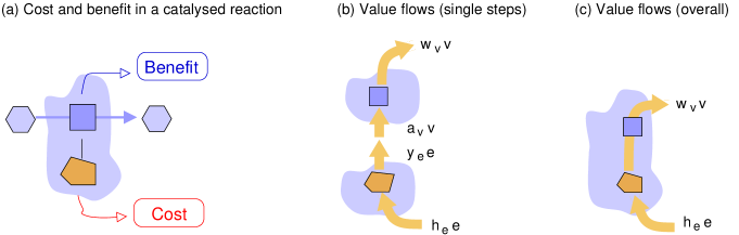
Figure 7: Conservation of economic value. (a) Example: a reaction (scored by a benefit function) and its catalysing enzyme (scored by a cost function). The subsystem considered is shown by a “cloud”. From Figure 2 we know that economic variables can be defined in two ways. Applying usual derivatives to benefit and cost functions yields values and prices, while applying scaled derivatives (also called “logarithmic” or “point derivatives”) leads to point benefits (also called “utilities” or “importances”) and point costs (or “investments”). Using these point derivatives, we can write all our economic laws in “value production form”, simply equating “inflowing” and “outflowing” values. (b) Value flows. Point costs and point benefits of enzyme (bottom) and reaction (top). Equation (31) tell us that all four quantities are equal (in optimal states). We can depict them as “value flows” entering and leaving our network elements. Value is “conserved” within each element, and also in between enzyme and reaction. (c) The same value flows can also be used to describe the coupled subsystem of reaction and enzyme (and any larger subsystems of metabolic networks, not shown).

9 The shape of economical metabolic flux profiles

What flux distributions can we expect to find in enzyme-optimal states? Some general features, which are independent of enzyme kinetics, follow from the variation condition Eq. (12). A flux profile that satisfies this equation with positive enzyme investments is called economical, and flux profiles must be economical to appear in enzyme-balanced states! Importantly, economical flux profiles are not just beneficial (${\bf b}_{\rm v}\cdot{\bf v}>0$), but must be locally beneficial: each enzyme must have a positive influence on the metabolic benefit. Uneconomical flux profiles entail a waste of enzyme, no matter which underlying kinetics or enzyme cost functions are assumed. How can we check in practice whether a flux profile is economical?

In the submode criterion for economic flux modes, we test for non-beneficial flux motifs, i.e.  local configurations of flux directions that would exclude an optimal usage of enzymes. A motif (or conformal submode) in a flux profile ${\bf v}$ is a set of active reactions that (by themselves) can carry a stationary flux with the same flux directions. Why do non-beneficial motifs make a flux profile noneconomical? The explanation is simple: in an optimal state, any flux variation must be fitness-neutral. Consider a flux variation $\delta{\bf v}$, caused by a change in enzyme levels that is itself a submode of ${\bf v}$. Applying this flux variation will increase some of the fluxes (but will not decrease any fluxes), so the enzyme demand increases. Since (constraint-respecting) variations in enzyme-balanced states must be fitness-neutral, the additional enzyme cost must be balanced by an extra benefit. This means: in an enzyme-optimal state, any conformal flux variations $\delta{\bf v}$ must be beneficial, and economical flux profiles cannot contain non-beneficial submodes! The submode criterion refers only to flux directions (and not to flux magnitudes) and can be used by comparing the flux profile to elementary futile submodes. If futile motifs are present, it is impossible to find economic potentials that satisfy the reaction balance; conversely, if no futile motifs are present, this guarantees that economic potentials can be found. Figure 8 shows an example: the flux profile in (a) contains, as a submode, the mode shown in (b). Since this submode is futile, the flux profile in (a) must be uneconomical and cannot be realised by enzyme-optimal models. The flux profile in (c), which does not contain the submode, is economical.

Figure 8: Futilre submodes and economical flux profiles. A flux profile is called economical if it can satisfy the flux variation rule (14) with positive enzyme investments. (a) Example pathway with production of metabolite B (blue circle) as the metabolic objective. The flux profile shown is uneconomical. We can see this by applying the submode criterion with the submode ${\boldsymbol{\kappa}}$ shown in (b). An economical flux profile cannot contain any futile submodes. Since this submode is futile (no B is produced) and conformal with the flux profile ${\bf v}$, ${\bf v}$ must be uneconomical. We can see this from the flux variation rule (14): since ${\bf b}_{\rm v}$ scores the production rate of B, the right-hand side ${\boldsymbol{\kappa}}\cdot{\bf b}_{\rm v}=0$ and the left-hand side ${\boldsymbol{\kappa}}\cdot({{\bf h}_{e}^{\centerdot}}/{\bf v})\neq 0$ cannot be equal. (c) Economical flux profile. To show that this flux profile is economical, we note that there are economic potentials (shades of blue) such that all fluxes lead from lower to higher potentials. In (a), for example, the flux cycle would make a consistent choice of economic potentials impossible. Note that the economic potentials of the external compounds A, B, C, and D are predetermined by the metabolic objective.

Economical flux profiles, as defined in kinetic models, are related to the principle of minimal fluxes [30], a heuristic rule in FBA. The principle of minimal fluxes states that a flux profile must satisfy the FBA constraints (stationarity and flux bounds), realise a given metabolic objective $b^{\prime}=\hat{{\bf b}}_{\rm v}\cdot{\bf v}$, and at the same time minimise the sum of absolute fluxes. Flux Cost Minimisation (FCM) [23] applies the same principle, but with general cost functions $a({\bf v})$ such as the sum of absolute fluxes $a({\bf v})=\sum|v_{l}|$ [30, 31] and the weighted sums of absolute fluxes $a({\bf v})=\sum\hat{a}_{v_{l}}|v_{l}|$ with cost weights $\hat{a}_{v_{l}}$ (or $a({\bf v})=\sum\hat{a}_{v_{l}}v_{l}$, if fluxes are known to be positive). An FCM problem is called flux-enforcing if its flux bounds exclude the equilibrium state ${\bf v}=0$ (by positive lower or negative upper flux bounds). In the corresponding FCM problems, shadow gains in the vector ${\bf b}_{\rm v}$ will lead to different flux solutions. FCM and metabolic value theory lead to the same flux solutions: any non-flux-enforcing FCM problem yields an flux profile that is economical, and any economical flux profile can be obtained by some non-flux-enforcing FCM problem (see Proposition LABEL:th:theoremPMF1, “Nocturno principle”). Starting from an enzyme-balanced state (with flux gain vector ${\bf b}_{\rm v}$), we can construct many FCM problems with flux objectives $b({\bf v})={\bf b}_{\rm v}\cdot\,{\bf v}$ and different cost functions $a({\bf v})$. All this holds both for general FCM problems and for FCM problems with linear flux costs functions $a({\bf v})=\sum_{l}a_{v_{l}}^{\prime}\,v_{l}$ (for each given pattern of flux directions). Thus, any economical flux profiles can be predicted by linear FCM by choosing appropriate flux cost weights! In theory, by randomly choosing cost weights $a_{v_{l}}^{\prime}$ and computing the flux solutions, any economical flux profile can be found. We saw that enzyme-optimal states correspond to solutions of FCM, a nonlinear version of FBA. In FCM, fluxes are optimised for a minimal cost, which suppresses futile cycle fluxes. In enzyme optimisation, it is enzymes, not fluxes that are costly, but optimising the enzyme levels leads again to economical fluxes. So both methods restrict fluxes in the very same way (see Proposition LABEL:th:theoremPMF1 in SI), and this even holds if the metabolic objective in enzyme optimisation depends on metabolite levels: the reason is that the reaction balance (25), our criterion for economical flux profiles, does not depend on concentration prices. Interestingly, FCM problems yield solutions that capture metabolite costs! This also means that kinetic models can be used to justify FCM: for any FCM solution ${\bf v}$, there will be a kinetic model that realises these fluxes by optimal enzyme levels. Conversely, FCM (and even linear FCM) can be used to compute economical flux profiles to be realised in enzyme-optimal states.

Coming back to FBA, how can we make sure that our flux solutions can also be realised by kinetic models in enzyme-optimal states? An FBA problem assumes an objective $b({\bf v})={\bf b}_{\rm v}\cdot{\bf v}$ with a constant vector ${\bf b}_{\rm v}$. Given the model, we can consider the set of all possible kinetic models with the same network structure and flux gain vector $\partial b/\partial{\bf v}={\bf b}_{\rm v}$, and ask about their enzyme-optimal states. Can we restrict our FBA problem to flux distributions that occur in one of these states? Since FBA does not consider enzyme kinetics, this may seem difficult, bur in fact the only thing we need to do is to exclude non-economical fluxes. However, our criteria for economical fluxes – submode criterion and existence of compatible economic potentials and enzyme investments – do not depend on kinetics and can therefore be used in FBA. This is fairly simple: in addition to stationary fluxes, we need to determine economic potentials that satisfy the reaction balance (20). Like in thermodynamic FBA, we obtain an extra constaint that restricts possible flux modes to a number of segments in flux space (flux orthants or their lower-dimensional surfaces). In the resulting “Value Balance Analysis”, all flux solutions must be economical, i.e. they must satisfy a reaction balance with some choice of economic potentials. The external economic potentials follow from the objective function, while the internal potentials $w_{\rm r_{i}}^{\rm int}$ must be chosen to achieve a positive value production $({b_{v_{l}}}+\square w_{\rm r_{l}}^{\rm int})\,v_{l}>0$, which means that flux values and fluxes must have the same signs. Mathematically, the latter condition resembles the thermodynamic constraint between chemical potentials and flux directions [32], where economic and chemical potentials correspond to each other. In practice, economic FBA uses energetic and economic constraints simultaneously: unphysical and uneconomical metabolic flux profiles are excluded at the same time. Economic and thermodynamic constraints can shape fluxes in similar ways. For example, just like thermodynamics excludes thermodynamically infeasible cycles, the value production principle excludes futile cycles.

10 Kinetic models in enzyme-optimal states

A search for optimal metabolic states by numerical optimisation may lead to irrelevant local optima, for instance a zero-flux state in which all enzyme levels vanish and small expression increases would not pay off. To obtain meaningful optima, can we use metabolic value theory to construct kinetic models systematically in enzyme-balanced states? In fact, metabolic value theory was initially developed from a simple question: is there a systematic way to construct kinetic models in enzyme-optimal states, as a starting point for assessing optimal enzyme activity changes? We saw that enzyme-optimal states must come with consistent economic potentials and fluxes, which in turn requires the flux profiles to be economical. But how to obtain the economic potentials? If a given kinetic model with metabolic state $({\bf v},{\bf c},{\bf e})$, the economic potentials can be computed by taking derivatives. But can we turn this around? Can we choose an economical flux distribution and a set of economic potentials, and construct a kinetic model with exactly these fluxes and economic potentials? And will this model be enzyme-balanced, or even be enzyme-optimal?

Due to this proposition, if a metabolic network, a flux gain vector ${\bf b}_{\rm v}$, and an economical flux profile ${\bf v}$ are given, kinetic models with this flux profile and with optimal enzyme levels can be constructed (see SI sections LABEL:sec:reconstruction and SI LABEL:sec:realisekineticmodels). We proceed in two steps. In the first step, the steady-state phase, we choose thermodynamically feasible metabolite concentrations as well as economic potentials satisfying the reaction balance. To obtain biologically plausible economic potentials, we can use extra constraints, heuristic assumptions (e.g. similar point costs for all enzymes [15]), or data (e.g. by fitting economic potentials to proteomics data as proxies for enzyme costs). Inactive reactions are omitted from the model. In the second step, the kinetic phase, we determine economic loads $y_{c_{i}}$ and reaction elasticities ${E^{\rm v_{l}}_{{\rm c}_{i}}}$ satisfying ${\bf w}_{\rm c}^{\rm int}={\bf y}_{\rm c}-\mathbf{g}_{\rm c}$ and Eq. (23). However, after our arbitrary choice of economic potentials in step one, there may be no solution anymore with our given metabolite price vector $\mathbf{g}_{\rm c}$. To obtain a solution anyway, we allow for a (minimal) adjustment of $\mathbf{g}_{\rm c}$. We obtain a set of constraints that define kinetically feasible elasticities and choose (e.g. sample) the elasticities under these constraints. From the elasticities, all kinetic constants for the model can be constructed. Aside from its practical usage, this algorithm shows that any economical flux profile can be realised by some enzyme-balanced kinetic model. Whether these models are enzyme-optimal (i.e. dynamically and economically stable) has to be checked separately.

In our workflow for model construction we can integrate various types of data including metabolite concentrations, fluxes, kinetic constants, enzyme efficiencies, and protein cost. For example, we can choose economic potentials and enzyme investments that comply with proteomics data and protein sizes, and then realise the resulting economic state by a kinetic model. Model variables can either be sampled, optimised, or chosen based on experimental knowledge or heuristical rules. By sampling repeatedly, we obtain an ensemble of kinetic models, each realising our flux profile under all kinetic, thermodynamic, and economic constraints. Figure 9 shows an example, a model of central metabolism in yeast. To choose the economic potentials, I make the simple heuristic assumption that the enzyme investments are similar between all enzymes. Alternative assumptions would be that known enzyme levels are translated into enzyme investments to which economic potentials could be fitted [15], or flux burdens $a_{v_{l}}=h_{e_{l}}/(v_{l}/e_{l})\geq h_{e_{l}}/k_{\rm cat,l}$ are estimated from known $k_{\rm cat}$ values and enzyme sizes. Using Eqs (14) and (15), these burdens can be adjusted to satisfy all constraints of an enzyme-optimal state.

(a) Economic potentials in respiration	(b) Economic potentials in fermentation

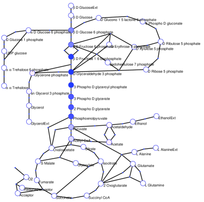
Figure 9: Economic potentials in the central metabolism of yeast, constructed from data and simple heuristic assumptions. (a) Economic potentials during respiration (usage of TCA cycle and oxidative phosphorylation). (b) Economic potentials during fermentation (with ethanol overflow). To reconstruct an enzyme-balanced state, I first determined thermodynamically feasible, economical fluxes by flux minimisation, where ATP production was used as the metabolic objective and some flux directions were predefined. Then, chemical and economic potentials were chosen within predefined ranges and in line with the known flux directions: the two types of potentials have to decrease or increase, respectively, along the fluxes (circle colours: pink: negative; white: zero; blue: positive; cofactors not shown). Finally, economic loads and elasticities were chosen and the kinetic constants were computed.

Will enzyme-balanced states constructed as show above be enzyme-optimal? While an enzyme balanced state satisfies the necessary optimality conditions (ensuring stationary and enzyme-balanced states), an enzyme-optimal state also needs to satisfy sufficient optimality conditions (ensuring dynamically and economically stable states). In our construction, the necessary condition is satisfied via the cost-benefit balance Eq. (24). To satisfy the sufficient conditions, any small metabolic perturbations must be buffered by the system dynamics, and any small enzyme variation must lead to a (second-order) fitness decrease. Thus, in a second-order approximation, Jacobian matrix and fitness curvature matrix ${\bf F}_{\rm uu}=\partial^{2}{\mathcal{F}}/(\partial e_{l}\,\partial e_{k})$ for active enzymatic reactions must be negative definite. The latter criterion, called “economic stability”, discards models with dynamically and economically unstable states, that is, models in local minima or saddle points of the fitness function. To find such models, we may construct enzyme-balanced models (as described above) and select those with dynamically and economically stable states (for details, see SI LABEL:sec:reconstructionbalanced). Economic stability may be formally ensured by strongly curved enzyme cost functions (entailing positive curvatures in all directions in enzyme space), but such cost functions may be biologically unrealistic.

11 Discussion

Metabolic value theory describes the value structure of metabolic states. Here we saw how economic variables and economic laws for kinetic metabolic models can be derived from Metabolic Control Theory. Figure 10 gives an overview. In optimal states, all active reactions must satisfy the cost-benefit balance Eq. (24). The value $y_{e_{l}}$ of an active enzyme (describing its effect on the metabolic objective) must be equal to the enzyme price $h_{e_{l}}$ and must therefore be positive. This principle leads to a number of other laws: using the summation and connectivity theorems of MCT, we obtain variation rules that relate flux gains to enzyme prices along a flux mode, and metabolite prices lead to the enzyme prices around the metabolite. In enzyme-optimal states, flux modes must be economical and thus free of futile motifs. Written in a local form, the variation rules yields economic rules and balance equations. The economic variables in these laws can be defined by metabolic control coefficients or shadow values [14] (proof in SI LABEL:sec:ProofsPotentialsAreIdentical). Extensions of the theory for models with other constraints or assumptions are described in appendix B.

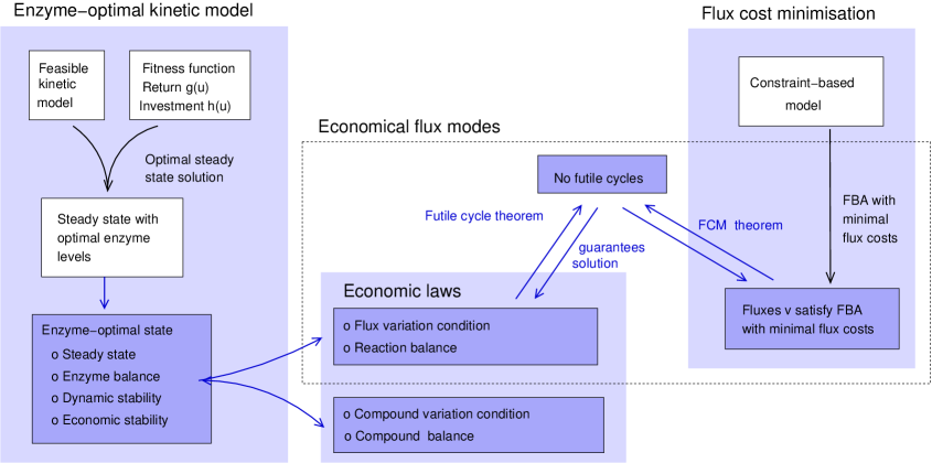
Figure 10: Economic laws for metabolic states. Conditions for kinetic models in enzyme-optimal states are shown on the left. For enzyme-balanced states, the necessary first-order conditions must be satisfied (stationary state and cost-benefit balance Eq. (24) describing a fitness extremum). For enzyme-optimal states, the sufficient second-order conditions must also be satisfied (dynamic stability, i.e. a negative definite Jacobian; and economic stability, i.e. a negative definite curvature matrix ${\bf F}_{\rm uu}$, ensuring a fitness maximum). From the necessary conditions follows a cost-benefit balance, entailing that active enzymes must have a positive control on the metabolic objective (“benefit principle”). This cost-benefit balance further leads to the variation rules (14) and (15) and to the economic balance equations (25) and (26). Economical flux profiles have convenient properties (dashed box): they satisfy the flux variation rule and the reaction balance, are free of futile motifs, are solutions of FCM problems, and satisfy a reaction balance with positive enzyme investments (right box).

So what did we learn about our initial questions?

1. The enzyme levels in optimal states depend on network-wide fitness requirements. In metabolic value theory, these requirements are described by local economic variables. More generally, we saw that the values of metabolites, enzyme, and reactions (describing their “network-wide” fitness effects) satisfy local balance relations resembling Kirchhoff’s rules for electric circuits. Using these rules, the indirect values and therefore the entire value structure can be inferred from direct gains and prices (describing direct effects of network elements on fitness) by projecting them onto the network.

2. A metabolic pathway can be seen as a value chain: the enzymes (and substrates) invested lead to increasing metabolite values along the pathway flux. All these investments are defined as “point costs” and measured in fitness units, which makes them comparable. The embodied investment of a metabolite, divided by the metabolite’s (absolute) production rate, defines its embodied value.

3. Flux profiles in enzyme-optimal states must follow some simple algebraic rules and must be solutions of FCM problems. Given an economical flux profile, we can construct enzyme-optimal states by (i) optimising the enzyme levels by ECM or by (ii) finding possible economic potentials and building kinetic models around them.

Economic values provide a new perspective on metabolic states. Kinetic models describe cells mechanistically by physical metabolic concentrations and fluxes. Thermodynamics adds a second layer of description, relating metabolite concentrations and fluxes by a notion of energies (in chemical potentials and thermodynamic forces). Metabolic value theory adds a third layer: a value structure described by economic variables. The economic potentials describe the use value of metabolites, as defined through the fitness effects of hypothetical state variations. The same logic applies generally: by writing physical laws as constaints, all physical variables can be associated with dual economic variables. The economic laws for these values allow us to study the value structure of metabolic states even if many model details are unknown. For example, we can explore the space of enzyme-balanced states, even without knowing the rate laws or enzyme cost functions. After constructing feasible economic states from the balance equations, we can realise them by enzyme-balanced kinetic models.

The elasticities and control coefficients in metabolic control theory exist in scaled and unscaled form. Likewise, the economic laws can be written in different forms, referring to fitness derivatives (“values” $f_{x}=\partial f/\partial x$), fitness contributions (“point derivatives” $f^{\centerdot}=\partial f/\partial\ln x=\partial f/\partial x\cdot x$), or differential fitness contributions (“variations” $\delta f=\partial f/\partial x\,\cdot\delta x$). For example, the point costs $h_{e_{l}}^{\centerdot}$ (or “enzyme investments”) are logarithmic derivatives describing costly effects of (actual or virtual) enzyme changes. This “marginal” definition of enzyme cost and benefit, describing changes of a given cell state, resembles the empirical definition in experimental studies [4, 25]. Conveniently, point derivatives can be obtained by multiplying each economic variable with the corresponding physical variable. If we do the same to our economic laws, we obtain economic laws in “value production forms”. In most cases, for going from “value form” (with values and prices) to “value production form” (with point benefits and point cost), we just need to put dots on the economic variables and replace elasticities by scaled elasticities.

Economic values are related to enzyme kinetics and metabolic control. Like control coefficients, the indirect enzyme values are not fixed molecule properties, but vary between metabolic states: they depend on an enzyme’s location in a metabolic network, on the fitness function, on metabolic fluxes, and on resource allocation between different enzymes. In optimal states, enzyme values must match enzyme prices $h_{e_{l}}$, which may be constant (in models with linear enzyme cost functions) or increase with increasing enzyme levels (assuming convex cost functions). In fact, metabolic value theory is an inverted form of MCT. While MCT describes the forward effects of enzyme changes (on the metabolic state), metabolic value theory turns this logic around and quantifies the incentives for enzyme changes, given a desired effect on a metabolic objective. In other words: to define metabolic values, we need to start from the desired objective and go back to necessary enzyme and metabolite changes. The flux gains, concentration prices and enzyme prices describe how an objective is directly affected by fluxes and concentrations. In the network, they indicate where cost and benefit are actually realised. If we start from there and follow the causal chains in reverse, we obtain the flux values, economic potentials, economic loads, and enzyme values that are indirectly promoted by the fitness function and acquired (in reverse direction) along causal chains. Therefore, causality (describing forward effects) and incentives (describing effects in reverse) are closely related, and this is why MVT can be based on MCT.

Metabolic dynamics arises from an interplay between metabolite concentrations and rates, via mass balances and kinetics. In MCT, fluxes within a flux mode are described by summation theorems, while concentrations (e.g. of a metabolite and the surrounding enzymes) are described by connectivity theorems. The two theorems hold independently. Similar complementary laws exist also in metabolic value theory: there is an economics of metabolite production (described by flux gains and economic potentials) and an economics of metabolite concentrations (described by concentration prices and economic loads). The economics of production concerns processes (including metabolite conversion, fluxes and metabolite net rates) and describes them by two sets of laws: from the flux variation rule, we obtain the reaction balance. The economics of concentrations concerns substance concentrations: the metabolite variation rule refers to concentration prices $\mathbf{g}_{\rm c}$ and gives rise to the metabolite balance. The two sets of conditions hold simultaneously, but can be studied separately. In flux analysis, for example, we may consider the reaction balance as a constraint, while ignoring metabolite concentrations. This allows us to determine feasible flux patterns and economic potentials without worrying about concentrations or specific kinetics model in which these potentials are defined.

The definition of metabolic values by metabolic control can help us make sense of the relation between control coefficients and enzyme levels [3]. For flux maximisation at a fixed enzyme budget, Klipp and Heinrich proved two kinds of relationships that hold in optimal states. First, the unscaled flux response coefficients $R^{\rm V}_{l}=\partial v^{\rm st}/\partial e_{l}$ must be equal. Second, the scaled flux control coefficients $\hat{C}^{\rm V}_{l}=\partial\ln|v^{\rm st}|/\partial\ln e_{l}$ must be proportional to the enzyme levels $e_{l}$. These relationships correspond exactly to our economic laws. The first relationship reflects the price-value balance $y_{e_{l}}=h_{e_{l}}^{\prime}$: if the cost function is given by the sum of enzyme levels, all enzymes have equal prices and must therefore have the same value. The second relationship reflects the cost-benefit balance $y_{e_{l}}\,e_{l}=h_{e_{l}}\,e_{l}$: if enzyme prices are fixed, enzyme levels are proportional to enzyme investments and therefore to enzyme point benefits (or “value production”). Thus, metabolic value theory confirms the relations from [3].

First, the equality $w_{v_{l}}\,v_{l}=y_{e_{l}}\,e_{l}$ from Eq. (31) reflects the fact that the scaled enzyme response coefficients and scaled control coefficients are equal [11]. Second, there is an interesting relation between flux burdens and control coefficients: in optimal states, the flux burden vector ${\bf a}_{\rm v}=\mbox{\rm Dg}({\bf h}_{\rm e})\,{\bf k}^{-1}$ is equal to the vector of flux values ${\bf w}_{\rm v}$ and must therefore be a nullvector of the matrix $(\mathbf{I}-{{\bf C}^{\rm v}})^{\top}$ (see SI LABEL:sec:SIproofsFluxPricesNullVector). This is interesting news for FCM, where ${\bf a}_{\rm v}$ is the gradient of the flux cost function. If the cost function is linear (as in FBA), (i.e. if ${\bf a}_{\rm v}$ is constant and predefined), the predefined ${\bf a}_{\rm v}$ puts constraints on the control coefficients in the underlying kinetic model, assuming an optimal system state.

If the enzyme prices $h_{e_{l}}$ are known (e.g. given by molecular masses), the proteome (vector ${\bf e}$) defines an investome. Simple cost-benefit principles tell us which enzymes should be expressed, and at what relative levels. Assuming an optimal state, enzymes must satisfy the value-price balance $k_{l}\,w_{v_{l}}=h_{e_{l}}$. If an enzyme efficiency $k_{l}$ is low (e.g. because of a low substrate level or a reaction close to chemical equilibrium), this balance cannot be satisfied and the enzyme should not be expressed. Likewise, for reactions with low or negative flux value $w_{v_{l}}$ (control over the metabolic objective), the condition cannot be satisfied. If enzymes are expressed, we may ask about expression levels. Any pair of enzymes must satisfy the relation $\frac{{h_{\rm e}}_{1}}{{h_{\rm e}}_{2}}=\frac{{y_{\rm e}}_{1}}{{y_{\rm e}}_{2}}=\frac{{w_{\rm v}}_{1}\,k_{1}}{{w_{\rm v}}_{2}\,k_{2}}$: if two enzymes share the same flux $v_{1}=v_{2}$ and if this flux is the metabolic objective, we obtain the relation $\frac{C^{\rm v}_{1}}{C^{\rm v}_{2}}\frac{e_{2}}{e_{1}}=\frac{{h_{\rm e}}_{1}}{{h_{\rm e}}_{2}}=\mbox{\rm const.}$ between the expression levels $e_{1}$ and $e_{2}$ (because $k_{l}=v_{l}/e_{l}$ and ${y_{\rm e}}_{l}=b_{J}\,C^{\rm v}_{i}$). Since this holds for any pair of enzyme, in optimal states, enzyme levels and flux control coefficients must be proportional, confirming the result by Klipp and Heinrich [3] for flux maximisation at a given total enzyme amount.

Metabolic Value Theory for general types of variables Also other model variables can be described by control coefficients, including peaks times in signaling system, the periods of metabolic oscillations, or the amplitudes of spatial modes in reaction-diffusion models. For a fitness-relevant target variable $x$, the control coefficients $\mathbf{C}^{x}_{v}$ and $\mathbf{C}^{x}_{r}$ can be used to define economic values, and if summation or connectivity theorems hold (e.g. proven by time-scaling arguments), these theorems yield economic laws.

Let us come back to our original question: how can we understand the quantitative proteome of a cell? In the introduction, I suggested that large protein investments must be justified by a large “importance”. of the protein. But what do we mean by “importance”? Transcription factors are important for cells, but their amounts are usually small. So if we claim that “investment equals importance”, we need to define our terms more precisely. We can paraphrase the result by Klipp and Heinrich by saying: if “investment” stands for enzyme amount, and “importance” stands the scaled flux control coefficient, investment and importance are balanced. “Enzyme investment” and “enzyme importance” will increase with the enzyme amount, and by dividing by this amount, we obtain a second equality, between “enzyme price” and “enzyme value”, the investment and importance per enzyme. Also this second equality follows from Klipp and Heinrich’s results if we define “enzyme price” as 1 (because all enzymes are weighted equally in the total enzyme amount, which needs to be minimised) and “enzyme value” by the unscaled response coefficient. Here we saw how these notions can be generalised: in metabolic value theory, an “enzyme price” is the derivative of an enzyme cost function, and “enzyme values” are response coefficients between enzyme levels and the metabolic objective. If we multiply price and value by the respective enzyme level, we obtain “investment” and “importance”.

To apply these notions to cell proteomes, we make three main assumptions: we assume, first, that each protein has a price (derived from some cost function to be specified, or maybe related to protein size); second, that enzymes contribute (indirectly) to a metabolic objective or benefit function (and that this contribution is described by control coefficients); and third, that the proteome represents an optimal state (where we can equate “importance=investment” and “value=price”). MVT yields critical insights about relation between enzyme and metabolite values: enzyme values are not “distributed at random”, but acquired from flux values, which in turn reflect economic potentials and flux gains. Thus, even if the enzyme values are unknown, we know in principle how they emerge from the metabolic network. If the enzyme prices are constant and known, we obtain strong constraints on the possible metabolite values. And in the “investment=importance” equality, then enzyme importance can be equated to a local value production (i.e. flux value times flux, or the balance value consumed and produced in reactions). Hence, the higher an enzyme level (assuming fixed prices), the higher must be the enzyme’s value production. All this shows that the proteome, which may appears structureless and “arbitrary” is in fact economically structured. If the metabolic network structure is known, we can use it to understand the “value structure” and make sense of the proteome.

Appendix A Mathematical details

A.1 Conformity criterion and submode criterion

To formulate the submode criterion for economical flux modes, we first need to define submodes and flux motifs. A flux distribution ${\boldsymbol{\kappa}}$ is conformal with another flux distribution ${\bf v}$ if all active reactions in ${\boldsymbol{\kappa}}$ are also active in ${\bf v}$ and show the same flux directions. Given a flux mode ${\bf v}$, a submode of ${\bf v}$ is a stationary flux mode ${\boldsymbol{\kappa}}$ on the subnetwork of active enzyme-catalysed reactions in ${\bf v}$ that is conformal with ${\bf v}$. The sign pattern of a submode is calle flux motif. In a model with flux gain vector ${\bf b}_{\rm v}$, a submode is either beneficial (${\bf b}_{\rm v}\cdot{\boldsymbol{\kappa}}>0$), futile (${\bf b}_{\rm v}\cdot{\boldsymbol{\kappa}}=0$), or wasteful (${\bf b}_{\rm v}\cdot{\boldsymbol{\kappa}}<0$).

The conformity criterion (Proposition LABEL:th:theoremtestmode in SI LABEL:sec:SIpropositions) for beneficial, futile, and wasteful submodes states the following: if ${\bf v}$ is an economical flux profile, then any beneficial submode ${\boldsymbol{\kappa}}$ must contain a reaction with the same flux direction as ${\bf v}$; any wasteful submode ${\boldsymbol{\kappa}}$ must contain a reaction with opposite flux directions in ${\boldsymbol{\kappa}}$ and ${\bf v}$; and any futile submode ${\boldsymbol{\kappa}}$ must contain both sorts of reactions. The conformity criterion follows from the flux variation condition Eq. (14), noting that $v_{l}$ and $v_{l}^{-1}$ have equal signs. Like the condition itself, it holds only for all-active flux profiles ${\bf v}$. If a flux profile ${\bf v}$ contains inactive reactions, these reactions must be omitted: flux gains ${b_{v_{l}}}$ and submodes ${\boldsymbol{\kappa}}$ must be within the active subnetwork.

The conformity criterion leads to the so-called submode criterion: all submodes of an economical flux profile must be beneficial, implying that a flux profile with futile or wasteful submodes is uneconomical. Also the opposite holds: according to proposition LABEL:th:theoremfutile (“conditions for economical flux profiles”), all flux profiles without non-beneficial submodes are economical. As a test for economical flux profile, we can simply search for futile and wasteful submodes. While the submode criterion holds for all futile submodes, it is safe to consider elementary futile submodes for practical tests: if a flux profile contains a non-elementary futile submode, it must also contain an elementary futile submode. Therefore, if a flux profile is free of elementary futile submodes, it is also free of any other futile submodes and is therefore economical.

A.2 Flux balance models and metabolite cost

How can flux cost minimisation models be reconciled with kinetic models? In fact, how is this possible at all? In FCM, costs are assigned to fluxes while metabolite concentrations are not described. In kinetic models, in contrast, the metabolic objective can depend both an fluxes and on metabolite concentrations. So how can both methods predict the same fluxes? Here is an explanation. In FCM we can choose a flux cost function that effectively describes enzyme and metabolite cost in a given kinetic model [23]. A linearised version of this function will captures enzyme and metabolite costs. If we use this cost function in linear FCM, we obtain shadow values (“economic potentials”) that refer to the sum of both costs. In fact, we can also turn this around: with any (feasible) set of economic potentials (e.g. no matter if we choose them by sampling, by adjusting them to proteomics data, or by assuming uniformly distributed enzyme investments), there will always exist an enzyme-optimal kinetic model that realises exactly these fluxes and economic potentials. Seen from an abstract perspective, metabolic value theory describes the economics of production rates (“production economics”) and the economics of concentrations (“concentration economics”), using separate variables (economic potentials versus loads) and economic laws (e.g. reaction balance versus metabolite balance, or flux variation condition versus metabolite variation condition). In practice, they can be used separately. Kinetic models contain two types of direct values, a flux gain vector ${\bf b}_{\rm v}$ and a concentration price vector $\mathbf{g}_{\rm c}$. Focusing on fluxes (e.g. in FCM problems), we may consider the “economics of conversion” while ignoring the “economics of concentrations”: we ignore metabolite concentrations and metabolite prices $g_{c_{i}}$ and describe fluxes and economic potentials relying on the reaction balance alone. The resulting fluxes will be realisable, at least, by some (unknown) kinetic model. Generally, there is a correspondence between models and states: each kinetic model yields a (consistent) set of fluxes and economic potentials, and any (consistent) fluxes and economic potentials represent, implicitly, an underlying kinetic model (or in fact, many of them) with specific enzyme kinetics and cost function. By first choosing consistent economic potentials and then reconstructing a kinetic model (or a range of kinetic models) that realises this profile, we can construct model ensembles.

A.3 Detailed conditions for optimal states

In our optimality problems for enzyme levels, metabolic objective $q({\bf v},{\bf c})$ and enzyme cost $h({\bf e})$ must be continuous functions, and the cost function must be bounded. We require that $h(\mathbf{e})\leq h^{\rm max}$, $h(\mathbf{e})\geq\hat{\mathbf{h}}_{e}\cdot\mathbf{e}$, and for pathway models we require that ${\mathcal{F}}(0)=0$, and ${\mathcal{F}}(\mathbf{e})>0$ for some $\mathbf{e}$. The existence of a local optimum can be proven easily: ${\mathcal{F}}$ has a positive maximum in the enzyme polytope defined by $\mathbf{e}\geq 0,\hat{h}_{e}\cdot\mathbf{e}\leq h^{\rm max}$. However, there may be multiple optimum points, which may also form a continuous manifold (e.g. in models with kinetically identical isoenzymes). Aside from physiologically plausible states, there may be a “locked state” at $\mathbf{e}=0$, describing an inactive system in which fluxes and enzyme levels vanish. Despite its low fitness, this locked state can be a locally optimal: an “economic barrier” for enzyme levels must be overcome to reach more profitable states. Only at higher enzyme levels, the system reaches the basin of attraction of a more profitable enzyme-balanced state. Finally, enzyme space may contain regions with infeasible enzyme profiles, for which no steady state exists (see SI LABEL:sec:importancereversible).

Appendix B Extending the theory

The models above depict cells in a simplified way: reactions are enzyme-catalysed and enzymes are fully specific, there are no isoenzymes, enzyme profiles are static and lead to stable steady states, the metabolic objective is a function of fluxes and metabolite concentrations, and enzyme levels are the control variables to be optimised. In reality, things are more complicated: cells show complex dynamics, are subject to other objectives and constraints, and may behave non-optimally. For a realistic picture of cells, our formalism can be extended in various ways (for details, see SI LABEL:sec:extensions).

(i) Isoenzymes and unspecific enzymes Our premise “one reaction, one enzyme” is not very realistic: biochemical reactions may be catalysed by more than one enzyme (isoenzymes), and enzymes may catalyse multiple reactions (unspecific or multifunctional enzymes). In models this leads to a non-diagonal enzyme elasticity matrix, which may not be invertible, and some formulae need to be modified. To convert $(\square w_{r_{l}}+{b_{v_{l}}^{\rm int}})\,{E^{\rm v_{l}}_{\rm e_{l}}}=h_{e_{l}}$ into $(\square w_{r_{l}}+{b_{v_{l}}^{\rm int}})\,v_{l}=h_{e_{l}}\,e_{l}$, we assumed that $\mathbf{E}_{\rm e}$ can be split into $\mathbf{E}_{\rm e}=\mbox{\rm Dg}({\bf v})\mbox{\rm Dg}({\bf e})^{-1}$. This allows us to move $\mbox{\rm Dg}({\bf e})$ to the right side, leading to separate equation for each reaction. If $\mathbf{E}_{\rm e}$ is not diagonal, this is not possible, and all we can do is write $\mathbf{E}_{\rm e}=\mbox{\rm Dg}({\bf v})\,{\mathbf{\hat{E}}^{\rm v}_{\rm e}}\,\mbox{\rm Dg}({\bf e})^{-1}$. Now , we obtain $\sum_{l}(\square w_{r_{l}}+{b_{v_{l}}^{\rm int}}),v_{l}\hat{E}^{v_{l}}_{e_{j}}=h_{e_{j}}\,e_{j}$, still with $\mbox{\rm Dg}({\bf v}){\mathbf{\hat{E}}^{\rm v}_{\rm e}}$ on the left, and the reactions remain economically coupled. In this new reaction balance equation, the effects of an unspecific enzyme are captured by summing over its catalysed reactions (see SI LABEL:sec:isoenzymes). The metabolite balance remains unchanged, but the elasticities between unspecific enzymes and their catalysed reaction are lower because an enzyme needs to split its activity between several reactions.

(ii) Economic balance equations for other cell variables The balance equations (25) and (26) refer to two basic motifs in metabolic networks: a reaction together with its reactants, and a metabolite together with the reactions it influences kinetically as a substrate, product, or effector. But there can also be other variables that affect reaction rates (such as temperature, membrane potentials, etc), and the associated economic values will satisfy balance equations. A costly control variable $p$ that affects a single reaction (with price $h_{p}$ and elasticity $E^{\rm v}_{p}$) leads to the balance equation $w_{v_{l}}\,v_{l}=h_{p}\,p/\hat{E}^{\rm v_{l}}_{{\rm p}}$. In general, several variables may affect a reaction, and several reactions may be affected by one variable. In the first case, we can sum the balance equations for the variables $p_{n}$ and obtain a balance between flux value and weighted average price $w_{v_{l}}=\langle h_{p_{n}}/{E^{\rm v_{l}}_{{\rm p}_{n}}}\rangle_{r}$ (proof: from $\sum_{n}w_{v_{l}}\,v_{l}=\sum_{r}h_{p_{n}}\,p_{n}/\hat{E}^{\rm v_{l}}_{{\rm p}_{r}}$ follows $w_{v_{l}}\,v_{l}=\frac{1}{N}\sum_{n}h_{p_{n}}\,p_{n}/\hat{E}^{\rm v_{l}}_{{\rm p}_{n}}$). In the second case, we can sum over the balance equations for different reactions and obtain a balance between elasticity-weighted average flux value and price, $\sum_{l}w_{v_{l}}\,{E^{\rm v_{l}}_{{\rm p}_{r}}}=h^{\rm p}_{r}$ (proof: $\sum_{l}w_{v_{l}}\,v_{l}\,\hat{E}^{\rm v_{l}}_{{\rm p}_{r}}=h^{\rm p}_{r}\,p_{r}$).

(iii) Choice variables besides enzyme levels In the models so far, metabolite concentrations and fluxes were treated as state variables and enzyme levels as control variables. But if our network also contains macromolecule synthesis (protein production, mRNA transcription, protein translation, or protein degradation), all macromolecules (including enzymes) should be described as metabolites. This is possible: other variables, such as mRNA levels, cell growth rate, temperature, concentrations in the extracellular medium, or administered drug levels may be used as control variables.

(iv) Constraints on state variables Cell physiology puts limits on enzyme concentrations, metabolite concentrations, and fluxes. Concentrations may be bounded by limited space or a cell may require some minimum ATP level or minimum maintenance flux to survive. In our optimality problems, such bounds can be treated as constraints, and the resulting shadow values of shadow prices appear as terms in the balance equations and can be included in ${\bf b}_{\rm v}$, $\mathbf{g}_{\rm c}$, and ${\bf h}_{\rm e}$ (SI LABEL:sec:inequality_constraints). For example, consider the constraint $e_{l}\geq 0$ for positive enzyme levels. If an enzyme is not expressed, this constraint is active, and if we include the Lagrange multiplier as a negative enzyme shadow price $-{h_{e_{l}}^{\rm bnd}}$ into the cost-benefit imbalance $y_{e_{l}}<h_{e_{l}}$, we obtain an equality $y_{e_{l}}=h_{e_{l}}-h_{e_{l}}^{\rm bnd}$. Similarly, constraints on fluxes or metabolite concentrations lead to shadow flux gains or prices. For example, if an ATP-consuming maintenance reaction is constrained to show some positive flux, this leads to a (positive) shadow gain which adds to the flux gain and contributes to the flux value of the reaction. In the flux benefit balance, this shadow gain can justify a non-zero flux even if the reaction consumes ATP without any benefit. Similarly, upper bounds on the enzyme abundance in cells, compartments or membranes (e.g. constraining the amount of photosystem complexes or ATP synthases) lead to shadow values, which add to the enzyme prices.

(v) Soft constraints on enzyme levels Metabolic limitations may either be described by constraints or by cost terms. For enzyme levels, instead of putting a constraint $e_{l}\geq 0$, we may add a cost that increases to infinity as $e_{l}$ goes to zero. This cost may also have a biological meaning. For example, if protein expression is leaky, and completely suppressing this is energy-demanding, this can be described by a penalty on very small enzyme levels. The resulting negative price for small enzyme levels replaces the shadow price that we get from hard constraints. With this cost term, enzymes will be expressed, but possibly at very low expression levels (see SI LABEL:sec:boundaryoptimaavoidedleaky).

(vi) Cost of unreliable enzyme expression Due to stochastic gene expression, protein molecule numbers follow random distributions and optimal enzyme levels can never be realised precisely. In a finite cell volume and assuming a Poisson distribution for enzyme molecule numbers $n$, the mean and standard deviation are given by $\bar{n}$ and $\sigma_{n}=\sqrt{\bar{n}}$, and the coefficient of variation $\sigma_{n}/\bar{n}=\sqrt{1/\bar{n}}$ decreases at higher (mean) expression levels. To guarantee sufficient enzyme levels despite this randomness, a cell may increase the mean enzyme level by adding a “safety margin”, for example $a$ times the standard deviation (and then fine-tuning enzyme activities by small-molecule regulation). If $n$ is Poisson-distributed and $\bar{n}$ is the desired expression value, the safe mean expression value would be $n+a\sqrt{n}$. The safety margin leads to a modified cost $h({\bf e}^{\prime})$, where ${\bf e}^{\prime}$ denotes a “safe” enzyme level $e^{\prime}=e+\frac{a}{\sqrt{N_{\rm A}\,V_{\rm cell}}}\sqrt{e}$, with Avogadro constant $N_{\rm A}$ and cell volume $V_{\rm cell}$. The relative increase due to the safety margin is highest at low expression levels. Unlike the usual cost functions (which are assumed to be linear or convex), the new cost function can be concave.

(vii) Inactive enzymes How does metabolic value theory describe inactive reactions? With a convex enzyme cost function (i.e. a non-decreasing enzyme price), the enzyme value of any inactive enzyme (with $v_{l}=0$) must be below the minimum enzyme price: then, expressing even small amounts of this enzyme (instead of none) would not pay off, but lead to a loss. Such reactions will remain inactive even under infinitesimal perturbations (e.g. of external metabolite levels) and can be ignored in the model. When constructing a model from given fluxes, zero fluxes can always be justified by assuming a high enzyme price. However, it is important to note that some main laws of metabolic value theory – the variation rules (12) and (13) and economic balance equations – hold only for all-active flux profiles: before applying them to a given flux profile, all inactive reactions must be omitted, also the in connection matrices such as ${\bf N}^{\rm int},{{\bf K}},{\bf L},\mathbf{E}_{\rm c}$, and test modes ${\boldsymbol{\kappa}}$ always refer to the active part of the network. Another way to model inactive reactions is to set enzyme levels to zero by explicit constraints. In the economic laws, the resulting shadow price $h_{e_{l}}^{\rm bnd}$ leads to an effective enzyme price $h_{e_{l}}=h_{e_{l}}+h_{e_{l}}^{\rm bnd}$. Alternatively, we can require an imbalance $y_{e_{l}}>h_{e_{l}}$ or a positive stress $t_{e_{l}}=y_{e_{l}}-h_{e_{l}}$ equal to $h_{e_{l}}^{\rm bnd}$. By inserting $y_{e_{l}}=w_{v_{l}}\,\frac{\partial v_{l}}{\partial e_{l}}$, we obtain the economic imbalance for fluxes, $w_{v_{l}}<h_{e_{l}}(\frac{\partial v_{l}}{\partial e_{l}})^{-1}=a_{v_{l}}$, that is, the flux value is below the flux burden.

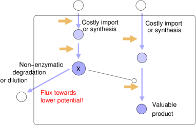
Figure 11: Non-enzymatic reactions with a seemingly uneconomical flux from high to low economic potentials. In the example, metabolite X acts as a catalyst and needs to be kept at its optimal concentration. Since X is non-enzymatically degraded or diluted, it needs to be reproduced. In its synthesis pathway, the economic potentials first increase, but then drop in the non-enzymatic reaction. In an enzymatic reaction such a drop would indicate a non-optimal state, so if we wrongly assume that our reaction is enzymatic, the flux distribution appears futile. However, in fact such pseudo-futile flux modes may be the best choice for a cell. To correctly classify them as economical, the flux variations in the flux variation rule (in the forms (10), ( 12), and (14)) must be restricted to enzymatic reactions.

(viii) Non-enzymatic reactions In metabolic models, non-enzymatic reactions are often ignored. However, but they can be important: they may degrade valuable metabolites, produce toxic compounds, or replace costly enzymatic reactions (e.g. membrane diffusion may replace costly transporters). Even if a reaction is uncatalysed, its flux can be indirectly controlled by surrounding enzymatic reactions. Therefore, the presence of non-enzymatic reactions creates new incentives that shape the optimal enzyme profile (see Figure 11 for an example). In our theory, to account for non-enzymatic reactions, some formulae need to be modified. (i) In the flux variation rules (10), (12), and (14), flux variations must comprise enzymatic reactions only. (ii) In the variation rules (LABEL:eq:fitnessbalance2 and (LABEL:eq:fitnessbalance3), extra terms for non-enzymatic reactions need to be added (see SI LABEL:sec:proofnonenzymatic). (iii) In the reaction imbalance Eq. (28), non-enzymatic reactions can be described by hypothetical enzymes with non-optimal concentrations (see SI LABEL:sec:violationsnonenzymatic) and by an imbalance term (or “tension”) $t_{e_{l}}^{\centerdot}=\partial{\mathcal{F}}/\ln e_{l}$ on the right side of the balance equation (see Eq. (28 ))). In beneficial non-enzymatic reactions, an imbalance $t_{e_{l}}^{\centerdot}$ denotes the minimal enzyme value at which this reaction would be profitable (if the enzyme existed). In contrast, a negative imbalance, describes the loss caused by the non-enzymatic reaction. (iv) In the metabolite balance (22), a non-enzymatic production, degradation, or dilution of the metabolite leads to extra terms, which can be seen as effective loads or concentration prices. (v) The definitions of economic potentials and loads as well as the reaction-metabolite balance remain unchanged.

(ix) Metabolite dilution In growing cells, dilution tends to decrease compound concentrations, as if all compounds were degraded by reactions with a linear rate law $\lambda\,c_{i}$ (where $\lambda$ is the cell growth rate). Dilution has effects on stationary fluxes, model dynamics, and cellular economics, including economic potentials and enzyme investments. In metabolic value theory, all results for non-enzymatic reactions also apply to dilution reactions, leading to simple formulae. Dilution reactions with rate constant $\lambda$ lead to an extra term $-\lambda\,\mathbf{I}$ in the Jacobian matrix, which reappears in the summation and connectivity theorems for control coefficients (SI LABEL:sec:SIproofMCAwithDilution), in the economic laws, and in some of the formulae for economic variables. To account for dilution in the metabolite balance (22) and in the reaction-metabolite balance (23), we consider an effective dilution reaction with flux $v^{\rm dil}_{i}=\lambda\,c_{i}$, elasticity $\lambda$, and a flux value $w_{\rm v_{i}}=-w_{\rm r_{i}}^{\rm int}$ (with a minus sign because the metabolite is “consumed”). We obtain the metabolite balance $y_{c_{i}}=\sum_{l}a_{v_{l}}\,{E^{\rm v_{l}}_{{\rm c}_{i}}}-\lambda\,w_{\rm r_{i}}^{\rm int}$. The new term $-\lambda\,w_{\rm r_{i}}^{\rm int}$ can be moved to the left and be included into the metabolite load, yielding the effective load $y_{c_{i}}^{\rm eff}=y_{c_{i}}+\lambda\,w_{\rm r_{i}}^{\rm int}$. Effectively, adding dilution increases the metabolite price by $\lambda\,w_{\rm r_{i}}^{\rm int}$. This makes sense: when a metabolite is diluted, lower concentrations lead to a lower value loss, thus creating an incentive for low concentrations: this resembles an extra metabolite price. Also in the metabolite variation rule, we can implement dilution by assuming an effective metabolite price $\mathbf{g}_{\rm c}^{\rm eff}=\mathbf{g}_{\rm c}+\lambda\,{\bf w}_{\rm r}^{\rm int}$ (SI LABEL:sec:demandDilution). The flux variation rule, in contrast, is not changed by dilution.

(x) Metabolic oscillations Mathematically, metabolic states with dilution are closely related to oscillating states [6]. This resemblance is useful if we model [33, 6, 14] metabolic oscillations in which oscillating metabolite concentrations and fluxes are enforced by oscillating enzyme activities. In an optimality problem, all oscillating variables are scored by a fitness function and our aim is to optimise enzyme amplitudes and phase angles for a maximal fitness. Oscillating metabolite concentrations and fluxes are approximated by sine waves (of circular frequency $\omega=2\,\pi\,f$), and their amplitudes and phases are described by complex-valued vectors ${\tilde{\bf c}}(\omega)$ and ${\tilde{\bf v}}(\omega)$. Instead of the usual stationarity condition ${\bf N}^{\rm int}\,{\bf v}=0$, we consider a mass balance equation $i\,\omega\,{\tilde{\bf c}}={\bf N}^{\rm int}\,{\tilde{\bf v}}$. Formally, the term on the left resembles a dilution term (with steady-state condition ${\bf N}^{\rm int}\,{\bf v}-\lambda\,{\bf c}=0$), with an imaginary number $\lambda=i\,\omega$ (with real-valued circular frequency $\omega$) instead of a real-valued dilution rate $\lambda$.

(xi) Multi-objective problems Multi-objective problems describe compromises between diferent objective functions. They can be used to describe organisms in changing environments, organisms anticipating uncertain challenges, and populations occupying several ecological niches in which all objectives are important, but to different extents in different niches. A “Pareto-optimal state” is a state in which no objective can be improved without compromising one of the other objectives. However, any Pareto-optimal state is also an extremal point of some single-objective problem (in which one target is optimised while constraining the others, or a convex combination of the different targets is optimised) [13]. Therefore, metabolic value theory can be applied to Pareto-optimal states [15].

References

- [1] J.G. Reich. Zur Ökonomie im Proteinhaushalt der lebenden Zelle. Biomed. Biochim. Acta, 42(7/8):839–848, 1983.
- [2] R. Heinrich and S. Schuster. The modelling of metabolic systems. Structure, control, and optimality. BioSystems, 47:61–77, 1998.
- [3] E. Klipp and R. Heinrich. Competition for enzymes in metabolic pathways: implications for optimal distributions of enzyme concentrations and for the distribution of flux control. BioSystems, 54:1–14, 1999.
- [4] E. Dekel and U. Alon. Optimality and evolutionary tuning of the expression level of a protein. Nature, 436:588–692, 2005.
- [5] W. Liebermeister, E. Klipp, S. Schuster, and R. Heinrich. A theory of optimal differential gene expression. BioSystems, 76:261–278, 2004.
- [6] W. Liebermeister. The economic basis of metabolic oscillations. Preprint on arXiv.org: arXiv:1602.05167, 2016.
- [7] E. Klipp, R. Heinrich, and H.-G. Holzhütter. Prediction of temporal gene expression. Metabolic optimization by re-distribution of enzyme activities. Eur. J. Biochem., 269:1–8, 2002.
- [8] A. Zaslaver, A.E. Mayo, R. Rosenberg, P. Bashkin, H. Sberro, M. Tsalyuk, M.G. Surette, and U. Alon. Just-in-time transcription program in metabolic pathways. Nature Genetics, 36:486–491, 2004.
- [9] W. Liebermeister, E. Noor, A. Flamholz, D. Davidi, J. Bernhardt, and R. Milo. Visual account of protein investment in cellular functions. PNAS, 111(23):8488–8493, 2014.
- [10] G.C. Brown. Total cell protein concentration as an evolutionary constraint on the metabolic control distribution in cells. J. theor. Biol., 153:195–203, 1991.
- [11] R. Heinrich and S. Schuster. The Regulation of Cellular Systems. Chapman & Hall, 1996.
- [12] J.-H.S. Hofmeyr and A. Cornish-Bowden. Regulating the cellular economy of supply and demand. FEBS Letters, 476(1-2):47–51, 2000.
- [13] W. Liebermeister. Optimal metabolic states in cells. Preprint on bioRxiv: DOI:10.1101/483867, 2018.
- [14] W. Liebermeister. The value structure of metabolic states. Preprint on bioRxiv: DOI:10.1101/483891, 2018.
- [15] W. Liebermeister. Metabolic economics in flux analysis: the principle of local value production. Preprint on arXiv.org: arXiv:1404.5072, 2014.
- [16] J.-H.S. Hofmeyr. Metabolic control analysis in a nutshell. In ICSB 2001 Online Proceedings, http://www.icsb2001.org/toc.html, 2001.
- [17] J. Uhlendorf. Prediction of optimal enzymatic regulation architectures. Master’s thesis, Department of Mathematics and Computer Science, Free University Berlin, 2009.
- [18] www.github.com/liebermeister/metabolic-economics.
- [19] S. Schuster and R. Heinrich. Minimization of intermediate concentrations as a suggested optimality principle for biochemical networks. Journal of Mathematical Biology, 29(5):425–442, 1991.
- [20] N. Tepper, E. Noor, D. Amador-Noguez, H.S. Haraldsdóttir, R. Milo, J. Rabinowitz, W. Liebermeister, and T. Shlomi. Steady-state metabolite concentrations reflect a balance between maximizing enzyme efficiency and minimizing total metabolite load. PLoS ONE, 8(9):e75370, 2013.
- [21] M. Scott, C.W. Gunderson, E.M. Mateescu, Z. Zhang, and T. Hwa. Interdependence of cell growth and gene expression: origins and consequences. Science, 330:1099, 2010.
- [22] M.T. Wortel, E. Noor, M. Ferris, F.J. Bruggeman, and W. Liebermeister. Metabolic enzyme cost explains variable trade-offs between microbial growth rate and yield. PLoS Computational Biology, 14(2):e1006010, 2018.
- [23] W. Liebermeister. Flux cost functions and the choice of metabolic fluxes. Preprint on arXiv.org: arXiv:1801.05742, 2018.
- [24] D.M. Stoebel, A.M. Dean, and D.E. Dykhuizen. The cost of expression of Escherichia coli lac operon proteins is in the process, not in the products. Genetics, 178(3):1653–1660, 2008.
- [25] I. Shachrai, A. Zaslaver, U. Alon, and E. Dekel. Cost of unneeded proteins in E. coli is reduced after several generations in exponential growth. Molecular Cell, 38:1–10, 2010.
- [26] M. Eames and T. Kortemme. Cost-benefit tradeoffs in engineered lac operons. Science, 336:911–915, 2012.
- [27] C. Reder. Metabolic control theory: a structural approach. J. Theor. Biol., 135:175–201, 1988.
- [28] H. Qian and D.A. Beard. Thermodynamics of stoichiometric biochemical networks in living systems far from equilibrium. Biophysical Chemistry, 114(2-3):213–220, 2005.
- [29] W. Liebermeister, J. Uhlendorf, and E. Klipp. Modular rate laws for enzymatic reactions: thermodynamics, elasticities, and implementation. Bioinformatics, 26(12):1528–1534, 2010.
- [30] H.-G. Holzhütter. The principle of flux minimization and its application to estimate stationary fluxes in metabolic networks. Eur. J. Biochem., 271(14):2905–2922, 2004.
- [31] H.-G. Holzhütter. The generalized flux-minimization method and its application to metabolic networks affected by enzyme deficiencies. BioSystems, 83:98–107, 2006.
- [32] A. Hoppe, S. Hoffmann, and H.-G. Holzhütter. Including metabolite concentrations into flux-balance analysis: Thermodynamic realizability as a constraint on flux distributions in metabolic networks. BMC Syst. Biol, 1(1):23, 2007.
- [33] W. Liebermeister. Response to temporal parameter fluctuations in biochemical networks. J. Theor. Biol., 234(3):423–438, 2005.