Large fluctuations in diffusion-controlled absorption

Abstract

Suppose that $N_{0}$ independently diffusing particles, each with diffusivity $D$, are initially released at $x=\ell>0$ on the semi-infinite interval $0\leq x<\infty$ with an absorber at $x=0$. We determine the probability ${\cal P}(N)$ that $N$ particles survive until time $t=T$. We also employ macroscopic fluctuation theory to find the most likely history of the system, conditional on there being exactly $N$ survivors at time $t=T$. Depending on the basic parameter $\ell/\sqrt{4DT}$, very different histories can contribute to the extreme cases of $N=N_{0}$ (all particles survive) and $N=0$ (no survivors). For large values of $\ell/\sqrt{4DT}$, the leading contribution to ${\cal P}(N=0)$ comes from an effective point-like quasiparticle that contains all the $N_{0}$ particles and moves ballistically toward the absorber until absorption occurs.

1 Problem Statement

When $N_{0}$ independent diffusing particles are released at $x=\ell>0$ on the infinite half-line $x>0$ with the origin being absorbing, a basic characteristic of the dynamics is the number of surviving particles. In this work, we focus on the distribution of the number of survivors at a specified time. As we shall discuss, disparate histories, that are very different from typical histories of diffusion, can contribute to the extreme cases where (a) all particles survive or (b) none survive.

The probability that a single particle survives up to time $t$ is

$$\overline{\Theta}(t)=\int_{0}^{\infty}c(x,t)\,dx\,,$$ (1)

where $c(x,t)$ is the probability density for the particle to be at position $x$ at time $t$ [1, 2]. This density obeys the diffusion equation

$$\partial_{t}c=D\,\partial_{x}^{2}c\,,$$ (2)

whose solution, subject to the initial condition $c(x,0)=\delta(x\!-\!\ell)$ and the absorbing boundary condition $c(0,t)=0$, is

$$c(x,t)=\frac{1}{\sqrt{4\pi Dt}}\left[e^{-\frac{(x-\ell)^{2}}{4Dt}}-e^{-\frac{(x+\ell)^{2}}{4Dt}}\right].$$ (3)

Then Eq. (1) gives

$$\overline{\Theta}(T)=\text{erf}\left(\frac{\ell}{\sqrt{4DT}}\right),$$ (4)

where $\text{erf}(z)=(2/\sqrt{\pi})\int_{0}^{z}e^{-u^{2}}\,du$ is the error function. Since the particles are non-interacting, the average number $\overline{N}(T)$ of survivors at $t=T$, when there are $N_{0}$ particles initially at $x=\ell$, is

$$\overline{N}(T)=N_{0}\,\overline{\Theta}(T)=N_{0}\;\text{erf}\left(\frac{\ell}{\sqrt{4DT}}\right).$$ (5)

Our goal is to determine the probability ${\cal P}(N)$ to observe any number of surviving particles $0\leq N\leq N_{0}$ at a specified observation time $t=T$. We shall also seek the most likely density history of the system, conditional on the survival of exactly $N$ particles at $t=T$. The number of survivors can be equal to $N_{0}$ (all particles survive until $t=T$) or to $0$ (no survivors). As we shall see, the relevant histories can be quite unusual in these cases and depend on the basic parameter $\ell/\sqrt{4DT}$.

Since the particles are independent, the probability ${\cal P}(N)$ can be found exactly from a microscopic theory, as given in the next section. The most likely history of the system is harder to find from microscopic arguments, even for independent particles. This history can be readily found, however, within the framework of the approximate macroscopic fluctuation theory of Bertini et al. [3, 4], which identifies the typical number of particles in the relevant region of space as the large parameter. As will be presented in Sec. 3, this most likely density history provides fascinating insights into the nature of large fluctuations in diffusion-controlled absorption.

2 ${\cal P}(N)$ and its limiting behaviors

The probability $\overline{\Theta}(T)$ that a single particle does not hit the absorber by time $T$ (the survival probability) is given by Eq. (4). The complementary probability that a single particle hits the absorber by time $T$ is $1-\overline{\Theta}(T)$. Since the particles are independent, the probability that exactly $N$ out of $N_{0}$ particles survive up to time $T$ is given by the binomial distribution:

$${\cal P}(N)=\binom{N_{0}}{N}\big{[}\overline{\Theta}(T)\big{]}^{N}\big{[}1-\overline{\Theta}(T)\big{]}^{N_{0}-N}.$$ (6)

In particular,

$${\cal P}(N\!=\!N_{0})=\left[\overline{\Theta}(T)\right]^{N_{0}}\qquad\text{and}\qquad{\cal P}(N\!=\!0)=\left[1-\overline{\Theta}(T)\right]^{N_{0}}.$$ (7)

Figure 1 shows $\ln{\cal P}$ versus $N$ for $N_{0}=30$ and three values of the parameter $\ell/\sqrt{4DT}$. For $\ell/\sqrt{4DT}=2$, corresponding to the situation where a particle typically has not yet diffused to the origin, the survival probability is peaked at the initial value $N=N_{0}=30$ and rapidly decreases as $N$ gets smaller. In the intermediate case of $\ell/\sqrt{4DT}=1/2$, where a particle has typically just diffused to the origin, the survival probability is peaked at $N=16$ and nearly symmetric apart from the tails. As one might expect, roughly one-half of the particles have been absorbed at this point. Finally, for $\ell/\sqrt{4DT}=1/10$, most of the particles have been absorbed. Here, the survival probability is peaked at $N=3$ and rapidly decreases as $N$ increases.

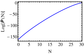
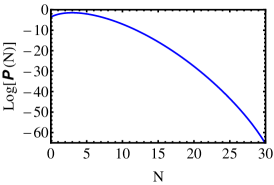
Figure 1: Logarithm of the survival probability ${\cal P}$ versus $N$ for $N_{0}=30$ and three values of $\ell/\sqrt{4DT}$: (a) 2, (b) $1/2$ and (c) $1/10$.

To elucidate the role of the parameter $\ell/\sqrt{4DT}$, we focus on two extreme cases: $N=N_{0}$ (all particles survive until $t=T$) and $N=0$ (no survivors at $t=T$), as well as the intermediate case with roughly similar numbers of survivors and non-survivors, $N_{0}\gg 1$, $N\gg 1$ and $N_{0}-N\gg 1$.

2.1 All particles survive until time $T$ ($N=N_{0}$)

For $\ell/\sqrt{4DT}\gg 1$, we use the asymptotic

$$\text{erf}\,z\simeq 1-\frac{e^{-z^{2}}}{\sqrt{\pi}z},\qquad z\gg 1\,,$$ (8)

to give

$$\ln{\cal P}(N\!=\!N_{0})\simeq-\frac{N_{0}\sqrt{4DT}}{\sqrt{\pi}\ell}\,\,e^{-\frac{\ell^{2}}{4DT}}~{}.$$ (9)

The right-hand side is extremely small so that ${\cal P}(N\!=\!N_{0})$ is extremely close to 1. This is expected as, for $\ell/\sqrt{4DT}\gg 1$, a particle typically travels a distance much smaller than $\ell$ during time $T$. Conversely, when $\ell/\sqrt{4DT}\ll 1$, we use the asymptotic $\text{erf}(z)\simeq(2/\sqrt{\pi})\,z$ to obtain

$${\cal P}(N\!=\!N_{0})\simeq\left(\frac{\ell}{\sqrt{\pi DT}}\right)^{N_{0}},$$ (10)

which is very small, again as expected.

2.2 No survivors at time $T$ ($N=0$)

In the limit of $\ell/\sqrt{4DT}\gg 1$, we obtain

$$\ln{\cal P}(N\!=\!0)\simeq-N_{0}\left(\frac{\ell^{2}}{4DT}+\ln\frac{\sqrt{\pi}\ell}{\sqrt{4DT}}+\dots\right),$$ (11)

so the probability is very small as expected. In the opposite limit of $\ell/\sqrt{4DT}\ll 1$, we obtain

$$\ln{\cal P}(N\!=\!0)\simeq-N_{0}\ell/\sqrt{\pi DT}.$$ (12)

The resulting probability can be close to or much less than one, depending on whether $N_{0}$ is small or large.

2.3 Intermediate case

For the situation where $N_{0}\gg 1$, $N\gg 1$ and $N_{0}-N\gg 1$, we use Stirling’s approximation in Eq. (6) to obtain, after some algebra,

$$-\ln{\cal P}(N)\simeq N_{0}\left[\Theta\ln\frac{\Theta}{\overline{\Theta}}+(1-\Theta)\ln\frac{1-\Theta}{1-\overline{\Theta}}\right]+\ln\left[\sqrt{2\pi N_{0}\,\Theta(1-\Theta)}\right],$$ (13)

where $\Theta=N/N_{0}$ is the fraction of surviving particles. Note that the survival probability $\overline{\Theta}=\overline{\Theta}(T)$, see Eq. (4), coincides with the expected (average) fraction of surviving particles. For $N$ close to its expected value, that is, for $\Theta$ close to $\overline{\Theta}$, the distribution ${\cal P}(N)$ is Gaussian:

$${\cal P}(N)\simeq\frac{1}{\sqrt{2\pi}\,\sigma}\,e^{-\frac{(N-\bar{N})^{2}}{2\sigma^{2}}}.$$ (14)

The variance is $\sigma^{2}=N_{0}\,\overline{\Theta}(1-\overline{\Theta})$. Interestingly, the fluctuations are maximal at an intermediate value of the parameter $\ell/\sqrt{4DT}$. Indeed, the variance $\sigma^{2}$ vanishes at $\ell/\sqrt{4DT}\to 0$ and $\ell/\sqrt{4DT}\to\infty$ [see Eq. (4)], and reaches a maximum value equal to $\sigma^{2}=N_{0}/4$ when $\overline{\Theta}=1/2$; that is, when $\ell/\sqrt{4DT}=0.4769\ldots$.

Notice that the first term on the right hand side of Eq. (13), which dominates $\ln{\cal P}(N)$, can be written in the scaling form

$$-\ln{\cal P}\simeq N_{0}\,\Phi\left(\frac{N}{N_{0}},\frac{\ell}{\sqrt{4DT}}\right).$$ (15)

Further, this first term alone correctly (and exactly) describes the extreme cases of $N=N_{0}$ and $N=0$, where the Stirling formula does not hold. In the following we shall rederive this dominant term within the framework of macroscopic fluctuation theory [3, 4]. This derivation will also yield the most likely density history of the system, a quantity that is not readily accessible by microscopic theory.

3 Macroscopic Fluctuation Theory

3.1 Basic Formalism

The macroscopic fluctuation theory (MFT) was originally developed and employed in the context of non-equilibrium steady states of diffusive lattice gases [3, 4, 5, 6] and subsequently extended to non-stationary settings [7, 8, 9, 10, 11, 12, 13]. The MFT, and its extensions to reacting particle systems [14, 15], has proven to be versatile and efficient. We briefly outline the (Hamiltonian form of the) MFT equations and refer the reader to the above references for details. For independent diffusing particles, the particle number density field $q(x,t)$ and the canonically conjugate “momentum” density field $p(x,t)$ obey Hamilton equations

$$\hskip 85.35826pt\partial_{t}q = D\partial_{x}^{2}q-2D\partial_{x}(q\partial_{x}p),$$ (16a)

$$\hskip 85.35826pt\partial_{t}p = -D\partial_{x}^{2}p-D(\partial_{x}p)^{2}.$$ (16b)

The Hamiltonian is $\int_{0}^{\infty}h\,dx$, where

$$h=-D\partial_{x}p\,\partial_{x}q+Dq(\partial_{x}p)^{2}.$$

The boundary conditions at the absorber at $x=0$ are $q(x\!=\!0,t)=p(x\!=\!0,t)=0$. The boundary conditions in time are the following. At $t=0$ we have

$$q(x,t\!=\!0)=N_{0}\delta(x-\ell).$$ (17)

The condition

$$\int_{0}^{\infty}q(x,T)\,dx=N$$ (18)

imposes an integral constraint on the solution; this setting is similar to that studied by Derrida and Gerschenfeld [9], see also Refs. [10, 12, 13]. A derivation, similar to that presented in Ref. [9], leads to the following boundary condition for $p$ at $t=T$:

$$p(x,t\!=\!T)=\lambda\theta(x),$$ (19)

where $\theta(x)$ is the Heaviside step function, and $\lambda$ is an a priori unknown Lagrange multiplier that is ultimately set by Eq. (18).

The solution of the MFT equations for $q(x,t)$ yields the most likely density history of the system that we seek. Once $q(x,t)$ and $p(x,t)$ are found, one can calculate the action $S$, which yields ${\cal P}(N)$ up to a pre-exponential factor:

$$-\ln{\cal P}\simeq S=D\int_{0}^{T}dt\,\int_{0}^{\infty}dx\,\left(p\partial_{t}q-h\right)=D\int_{0}^{T}dt\int_{0}^{\infty}dx\,q\,(\partial_{x}p)^{2}.$$ (20)

3.2 Hopf-Cole transformation and solution of the MFT problem

For independent diffusing particles, the MFT problem is exactly soluble via the Hopf-Cole transformation: a canonical transformation from $(q,p)$ to $Q=qe^{-p}$ and $P=e^{p}$ [14, 9, 11]. The generating function of this canonical transformation is

$$\int_{0}^{\infty}F(q,Q)\,dx=\int_{0}^{\infty}\left[q\ln(q/Q)-q\right]\,dx.$$ (21)

The transformed Hamiltonian is $\int H\,dx$, where

$$H=-D\,\partial_{x}P\,\partial_{x}Q\,.$$

In the new variables, the Hamilton equations for $Q$ and $P$ are decoupled:

$$\hskip 105.2751pt\partial_{t}Q = D\partial_{x}^{2}Q\,,$$ (22a)

$$\hskip 105.2751pt\partial_{t}P = -D\partial_{x}^{2}P\,.$$ (22b)

As shown in A, the action (20) can be written as

$$S\!=\!\int_{0}^{\infty}\!\!\!dx\left\{q(x,T)\Big{[}\ln\frac{q(x,T)}{Q(x,T)}\!-\!1\Big{]}-q(x,0)\Big{[}\ln\frac{q(x,0)}{Q(x,0)}\!-\!1\Big{]}\!+\!Q(x,T)\!-\!Q(x,0)\right\},$$ (23)

which is fully determined by the initial and final states of the system. However, to determine $Q(x,t)$ and $q(x,T)$, we need to find the entire phase trajectory of the system. Since Eqs. (22a) and (22b) are decoupled, we can solve the anti-diffusion equation (22b) backward in time, with the initial condition $P(x,T)=1+(e^{\lambda}-1)\theta(x)$ and the boundary conditions $P(0,t)=1$ and $P(\infty,t)=e^{\lambda}$. The solution is

$$P(x,t)=1+(e^{\lambda}-1)\,\text{erf}\left[\frac{x}{\sqrt{4D(T-t)}}\right].$$ (24)

At $t=0$ we obtain

$$Q(x,0)=\frac{q(x,0)}{P(x,0)}=\frac{N_{0}\,\delta(x-\ell)}{1+(e^{\lambda}-1)\,\text{erf}\left(\frac{x}{\sqrt{4DT}}\right)}=\frac{N_{0}\,\delta(x-\ell)}{1+(e^{\lambda}-1)\,\text{erf}\left(\frac{\ell}{\sqrt{4DT}}\right)}~{}.$$

This expression serves as the initial condition for solving the diffusion equation (22a) forward in time with the boundary conditions $Q(0,t)=q(0,t)/P(0,t)=0$ and $Q(\infty,t)=0$. The solution is

$$Q(x,t)=\frac{N_{0}}{\sqrt{4\pi Dt}}\,\frac{e^{-\frac{(x-\ell)^{2}}{4Dt}}-e^{-\frac{(x+\ell)^{2}}{4Dt}}}{1+(e^{\lambda}-1)\,\text{erf}\left(\frac{\ell}{\sqrt{4DT}}\right)}~{}.$$ (25)

We can now find $q(x,T)=Q(x,T)P(x,T)=e^{\lambda}Q(x,T)$ and evaluate the action in Eq. (23):

$$S=\frac{N_{0}\lambda e^{\lambda}\overline{\Theta}}{1+(e^{\lambda}-1)\overline{\Theta}}-N_{0}\log\left[1+(e^{\lambda}-1)\overline{\Theta}\right].$$ (26)

Now we use Eq. (18) to express $\lambda$ via $N$:

$$\frac{N_{0}e^{\lambda}\,\overline{\Theta}}{1+(e^{\lambda}-1)\,\overline{\Theta}}=N,$$

which yields

$$\lambda=\ln\left[\frac{\Theta(1-\overline{\Theta})}{(1-\Theta)\overline{\Theta}}\right].$$ (27)

Substituting Eq. (27) into (26), we obtain

$$-\ln{\cal P}\simeq S=N_{0}\left[\Theta\ln\frac{\Theta}{\overline{\Theta}}+(1-\Theta)\ln\frac{1-\Theta}{1-\overline{\Theta}}\right].$$ (28)

This expression coincides with the leading term of Eq. (13), which was obtained from the exact solution (6) in the regime $N_{0}\gg 1$, $N\gg 1$ and $N_{0}-N\gg 1$. By normalizing the approximate distribution (28) in the Gaussian region, we can also obtain the subleading term in Eq. (13) [but with $\overline{\Theta}(1-\overline{\Theta})$ instead of $\Theta(1-\Theta)$ inside the square root].

Now let us focus on the most likely density history, as described by $q(x,t)=Q(x,t)P(x,t)$. Using Eqs. (24), (25), (27) and (3), we obtain

$$q(x,t)=\frac{\overline{\Theta}(1-\Theta)+(\Theta-\overline{\Theta})\,\text{erf}\left[\frac{x}{\sqrt{4D(T-t)}}\right]}{\overline{\Theta}(1-\overline{\Theta})}\,\,q_{\text{mf}}(x,t),$$ (29)

where

$$q_{\text{mf}}(x,t)=N_{0}\,c(x,t)=\frac{N_{0}}{\sqrt{4\pi Dt}}\left[e^{-\frac{(x-\ell)^{2}}{4Dt}}-e^{-\frac{(x+\ell)^{2}}{4Dt}}\right]$$ (30)

gives the mean-field density history, which is not conditional on any number of survivors at $t=T$.

Equation (29), together with (6), are the main results of this work. Of particular interest is the density profile at $t=T$:

$$q(x,T)=\frac{N}{\overline{\Theta}\sqrt{4\pi DT}}\left[e^{-\frac{(x-\ell)^{2}}{4DT}}-e^{-\frac{(x+\ell)^{2}}{4DT}}\right].$$ (31)

By virtue of Eq. (30), we obtain

$$\frac{q(x,T)}{q_{\text{mf}}(x,T)}=\frac{N}{\overline{N}(T)}\,,$$ (32)

where $\overline{N}(T)$ is given by Eq. (5). The most likely density profile at $t=T$, conditional on $N$ particles surviving, differs from the unconditional profile, where $\overline{N}(T)$ particles have survived, only by the position-independent factor $N/\overline{N}(T)$. For $t<T$, however, the two density profiles are spatially quite dissimilar, as is evident from Eq. (29).

A particularly useful characteristic of the survival history is the most likely number of surviving particles $n(t)$ at intermediate times $0<t<T$, conditioned on there being exactly $N$ survivors at $t=T$. To evaluate this quantity, we transform the particle flux in Eq. (16a) to the new variables $Q$ and $P$:

$$j(x,t)=-D\partial_{x}q+2Dq\partial_{x}p=DQ(x,t)\partial_{x}P(x,t)-DP(x,t)\partial_{x}Q(x,t)\,.$$ (33)

Using Eqs. (24) and (25) for $P$ and $Q$, we evaluate $j(x\!=\!0,t)$ and integrate it over time from $0$ to $t$. The result is

$$\frac{n(t)}{N_{0}}=1-\left(1-\frac{N}{N_{0}}\right)\,\frac{\text{erfc}\left(\frac{\ell}{\sqrt{4Dt}}\right)}{\text{erfc}\left(\frac{\ell}{\sqrt{4DT}}\right)}~{},$$ (34)

where $\text{erfc}(z)=1-\text{erf}(z)$.

Now let us consider the two extreme examples already discussed in Sec. 2. For the subset of histories where all the particles survive up to time $T$, namely $N=N_{0}$, Eq. (29) becomes

$$q(x,t)=\frac{N_{0}}{\sqrt{4\pi Dt}}\left[e^{-\frac{(x-\ell)^{2}}{4Dt}}-e^{-\frac{(x+\ell)^{2}}{4Dt}}\right]\,\frac{\text{erf}\left[\frac{x}{\sqrt{4D(T-t)}}\right]}{\text{erf}\left(\frac{\ell}{\sqrt{4DT}}\right)}.$$ (35)

In this case, the optimal fluctuation acts to make the particle flux (33) zero at $x=0$ for all times $0<t<T$. For $\ell/\sqrt{4DT}\ll 1$, $q(x,t)$ in Eq. (35) becomes independent of $\ell$:

$$q(x,t)\simeq\frac{N_{0}\sqrt{DT}\,x\,e^{-\frac{x^{2}}{4Dt}}\,\text{erf}\,\left[\frac{x}{\sqrt{4D(T-t)}}\right]}{2(Dt)^{3/2}}\,.$$

In this regime, the survival of all particles until time $T$ can be achieved only as a result of a large fluctuation. Figure 2 compares the profiles of $q(x,t)$ and $q_{\text{mf}}(x,t)$ at different times for $\ell/\sqrt{4DT}=1/10$.

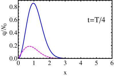
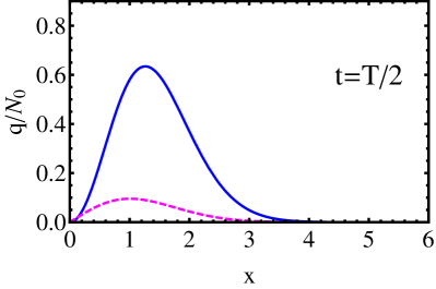
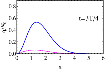
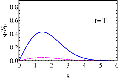
Figure 2: The most likely density history, conditional on survival of all $N_{0}$ particles by time $t=T$, Eq. (35) (the solid line). Also shown, by the dashed line, is the most likely unconditional density history, Eq. (30). The parameters are $\ell=1/5$, $T=1$ and $D=1$.

Even more interesting is the example of $N=0$, corresponding to no survivors at $t=T$. Now Eq. (29) becomes

$$q(x,t)=\frac{N_{0}}{\sqrt{4\pi Dt}}\left[e^{-\frac{(x-\ell)^{2}}{4Dt}}-e^{-\frac{(x+\ell)^{2}}{4Dt}}\right]\,\frac{\text{erfc}\left[\frac{x}{\sqrt{4D(T-t)}}\right]}{\text{erfc}\left(\frac{\ell}{\sqrt{4DT}}\right)}.$$ (36)

In this case, it is the regime of $\ell/\sqrt{4DT}\gg 1$ that is controlled by a large fluctuation. Figure 3 compares the profiles of $q(x,t)$ and $q_{\text{mf}}(x,t)$ at different times for $\ell/\sqrt{4DT}=5$. For this parameter value, the expected number of survivors is only slightly less than $N_{0}$. Here the density profile, conditional on no survivors at $t=T$, has the form of a relatively narrow pulse that moves toward the absorber and is absorbed at $t\simeq T$.

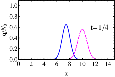
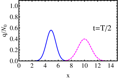
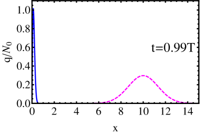
Figure 3: The most likely density profile history, conditional on extinction of all $N_{0}$ particles by time $t=T$, Eq. (35) (the solid line). Also shown, by the dashed line, the most likely unconditional density profile history, Eq. (30). The parameters are $\ell=10$, $T=1$ and $D=1$.

We now make these qualitative observations quantitative. For $\ell/\sqrt{4DT}\gg 1$, we use the large-argument asymptotic of $\text{erfc}\,(\ell/\sqrt{4DT})$ in Eq. (36), see Eq. (8). For not too small values of $x$, the large-argument asymptotic can also be used for the erfc function in the numerator of Eq. (36), and we can ignore the negligible second Gaussian in the square brackets. As a result,

$$q(x,t) \simeq\frac{N_{0}\ell}{x}\,\sqrt{\frac{T-t}{4\pi D\,t\,T}}\exp\left[-\frac{(x-\ell)^{2}}{4Dt}-\frac{x^{2}}{4D(T-t)}+\frac{\ell^{2}}{4DT}\right]$$

$$=\frac{N_{0}\ell}{x}\,\sqrt{\frac{T-t}{4\pi D\,t\,T}}\,\exp\left\{-\frac{T}{4Dt(T-t)}\,\left[x-x_{*}(t)\right]^{2}\right\},$$ (37)

where

$$x_{*}(t)=\ell(1-t/T).$$ (38)

The peak of this density pulse at $x\simeq x_{*}(t)$ moves ballistically toward the absorber with speed $\ell/T$, while the maximum density is

$$q_{\text{max}}(t)\simeq q_{*}[x_{*}(t),t]\simeq N_{0}\,\left[4\pi Dt(1-t/T)\right]^{-1/2}$$

and the characteristic pulse width, $\Delta(t)=\sqrt{Dt(1-t/T)}$. The pulse height decreases and the pulse width increases with time until $t=T/2$ and vice versa for $t>T/2$. The strong inequality $\ell/\sqrt{4DT}\gg 1$ guarantees that $\Delta\ll\ell$ at all times. Thus we can approximately replace $x$ by $x_{*}(t)$ in the prefactor of Eq. (3.2). This yields the Gaussian density profile

$$q(x,t)\simeq\frac{N_{0}}{\sqrt{2\pi}\,\Delta(t)}\,e^{-\frac{(x-x_{*})^{2}}{2\Delta^{2}(t)}},$$ (39)

that is generally valid except very close to $t=T$. To leading order, this solution describes a ballistically moving constant-mass quasiparticle. This ballistic motion arises because of the constraint that a large number of particles must be transported from $x=\ell$ to $x=0$ in a very short time. In this noise-dominated regime we can neglect the second derivatives in the MFT equations (16a) and (16b) to lowest order, leading to the reduced MFT equations [13]

$$\hskip 99.58464pt\partial_{t}q = -2D\partial_{x}(q\partial_{x}p),$$ (40a)

$$\hskip 99.58464pt\partial_{t}p = -D(\partial_{x}p)^{2}.$$ (40b)

Now we need to solve Eq. (40b) backward in time with the initial condition (19). In view of Eq. (27), the condition $N=0$ corresponds to $\lambda=-\infty$. That is, $p(x\!>\!0,T)\to-\infty$ as $t\to T$. The appropriate solution is (cf. Ref. [13])

$$\partial_{x}p(x>0,t)=-\frac{x}{2D(T-t)}\,.$$ (41)

Equation (40a) is a continuity equation for the density $q(x,t)$ with velocity field $2D\,\partial_{x}p$, with $\partial_{x}p$ determined from Eq. (41). As one can easily check, its exact (generalized, or weak) solution for the delta-function initial condition (17) is the translating delta function:

$$q(x,t)=N_{0}\,\delta[x-x_{*}(t)]\,,$$ (42)

with $x_{*}(t)$ given by Eq. (38). In this limit, the quasiparticle is simply a material point. Upon its release at $x=\ell$, this point moves ballistically with speed $\ell/T$ until it hits the absorber. Let us calculate the quasiparticle contribution to the action, using Eq. (20):

$$-\ln{\cal P}(N\!=\!0)=S =D\!\int_{0}^{T}\!\!dt\int_{0}^{\infty}\!\!dx\,q\,(\partial_{x}p)^{2}$$

$$=D\int_{0}^{T}\!\!dt\int_{0}^{\infty}\!\!dx\,N_{0}\,\delta[x-x_{*}(t)]\,\frac{x^{2}}{4D^{2}(T\!-\!t)^{2}}=\frac{N_{0}\ell^{2}}{4DT}.$$ (43)

This result coincides with the leading-order term in Eq. (11). That is, the dominant contribution to the action comes from a ballistically moving quasiparticle. A similar effect is observed when an unusually large mass or energy is transported in a short time in interacting diffusive lattice gases of the so-called hyperbolic class [12].

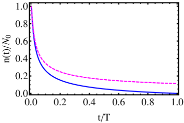
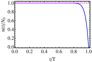
Figure 4: Solid line: the fraction of survivors $n(t)/N_{0}$ versus $t/T$, conditional on no survivors at $t=T$ for (a) $\ell/\sqrt{4DT}=1/10$ and (b) $\ell/\sqrt{4DT}=5$. Dashed line: the most likely unconditional fraction of survivors $\overline{\Theta}(t)$ from Eq. (4).

Finally, let us examine how the most probable number of particles $n(t)$ in Eq. (34) depends on time under the constraint that no particles survive at time $t=T$. Figure 4 shows the fraction of survivors $n(t)/N_{0}$ versus $t$ for: (a) $\ell/\sqrt{4DT}=1/10$ and (b) $5$. In the former case, most of the particles would get absorbed by $t=T$ “naturally”, without need for large fluctuations. In the latter case almost all particles would typically survive up to $t=T$, so a large fluctuation is needed to ensure that all of them are absorbed. The latter case corresponds to the evolution illustrated in Fig. 3, where a quasiparticle moves ballistically toward the absorber so that essentially all particles are absorbed when $t=T$.

4 Concluding Remarks

We investigated the role of large fluctuations in diffusion-controlled absorption in one dimension. We determined the probability distribution of the number of particles $N$ that have not been absorbed by time $T$. Apart from $N$ and $N_{0}$, this distribution crucially depends on the parameter $\ell/\sqrt{4DT}$.

We employed the macroscopic fluctuation theory (MFT) to find the “optimal path” of the system, namely, the most probable density history conditioned on a given number of surviving particles at an arbitrary observation time $t=T$. The optimal path gives fascinating insights into the nature of large fluctuations of the absorption process. A striking result arises in the situation where one demands that the particles, released far from the absorber, are absorbed in time $T$ that is short. Here, to leading order, the spatial probability density moves like a material point particle with constant speed towards the origin, and is absorbed at time $T$.

The model of non-interacting diffusing particles is amenable to a complete analytical solution within the framework of the MFT [14, 9, 11]. For diffusive lattice gases of interacting particles, the MFT problem becomes much harder to solve. Nevertheless, some of the insights we gained here should be useful in studying particle or energy absorption and other dynamical processes in interacting lattice gases.

We thank Paul Krapivsky for helpful discussions. Financial support of this research was provided in part by BSF grant No. 2012145 (BM and SR) and NSF Grant No. DMR-1205797 (SR).

Appendix A Action

The action can be written as

$$S = \int_{0}^{T}dt\int_{0}^{\infty}dx\left(p\partial_{t}q-w\right)$$ (44)

$$= \int dx\,F(q,Q)\biggl{|}_{0}^{T}+\int_{0}^{T}dt\int_{0}^{\infty}dx\left(P\partial_{t}Q+D\partial_{x}P\partial_{x}Q\right)$$

$$= \int dx\,F(q,Q)\biggl{|}_{0}^{T}+\int_{0}^{T}dt\int_{0}^{\infty}dx\left(DP\partial_{x}^{2}Q+D\partial_{x}P\partial_{x}Q\right)$$

$$= \int dx\,F(q,Q)\biggl{|}_{0}^{T}-\int_{0}^{T}\,dtP(0,t)D\partial_{x}Q(0,t).$$

As $p(0,t)=0$, we have $P(0,t)=1$. Using Eq. (22a), we obtain

$$-D\partial_{x}Q(0,t)=\int_{0}^{\infty}\partial_{t}Q\,dx.$$

Therefore, the last term in Eq. (44) can be written as

$$-\int_{0}^{T}\,dt\,P(0,t)D\partial_{x}Q(x,t)=\int_{0}^{T}dt\,\partial_{t}\int_{0}^{\infty}Q\,dx=\int_{0}^{\infty}dx\,Q(x,t)\biggl{|}_{0}^{T},$$

and we obtain Eq. (23) for the action.

References

- [1] G. H. Weiss, Aspects and Applications of the Random Walk (North-Holland, Amsterdam, 1994).
- [2] S. Redner, A Guide to First-Passage Processes (Cambridge University Press, Cambridge, 2001).
- [3] L. Bertini, A. De Sole, D. Gabrielli, G. Jona-Lasinio, and C. Landim, Phys. Rev. Lett. 87, 040601 (2001); J. Stat. Phys. 107, 635 (2002); Phys. Rev. Lett. 94, 030601 (2005); J. Stat. Phys. 123, 237 (2006).
- [4] G. Jona-Lasinio, Prog. Theor. Phys. Suppl. 184, 262 (2010); J. Stat. Mech. (2014) P02004.
- [5] J. Tailleur, J. Kurchan, and V. Lecomte, Phys. Rev. Lett. 99, 150602 (2007); J. Phys. A 41, 505001 (2008).
- [6] G. Bunin, Y. Kafri, and D. Podolsky, J. Stat. Mech. (2012) L10001, J. Stat. Phys. 152, 112 (2013).
- [7] B. Derrida, J. Stat. Mech. P07023 (2007).
- [8] P. I. Hurtado, C. P. Espigares, J. J. del Pozo, and P. L. Garrido, J. Stat. Phys. 154, 214 (2014).
- [9] B. Derrida and A. Gerschenfeld, J. Stat. Phys. 137, 978 (2009).
- [10] P. L. Krapivsky and B. Meerson, Phys. Rev. E 86, 031106 (2012).
- [11] P. L. Krapivsky, B. Meerson and P. V. Sasorov, J. Stat. Mech. (2012) P12014.
- [12] B. Meerson and P. V. Sasorov, J. Stat. Mech. (2013) P12011.
- [13] B. Meerson and P. V. Sasorov, Phys. Rev. E 89, 010101(R) (2014); A. Vilenkin, B. Meerson and P. V. Sasorov, J. Stat. Mech. (in press); arXiv:1403.7601.
- [14] V. Elgart and A. Kamenev, Phys. Rev. E 70, 041106 (2004).
- [15] B. Meerson and P. V. Sasorov, Phys. Rev. E 83, 011129 (2011).