Excited Coherent States Attached to Landau Levels

Abstract

A new scheme is proposed to design excited coherent states, $|\beta,\alpha;\mathbf{n}\rangle:={{{a^{{\dagger}}}^{\mathbf{n}}}|\beta,\alpha\rangle}$. Where the states $|\beta,\alpha\rangle$ denote the Glauber two variable minimum uncertainty coherent states, which minimize minimum uncertainty conditions while carrier nonclassical properties too and $\mathbf{n}$ is an integer. They are converted into the Agarwal’s type of the photon added coherent states, arbitrary Fock states and the Glauber two variable coherent states, respectively depending on which of the parameters $\alpha,\beta$ and $\mathbf{n}$ equal to zero. It has been shown that the resolution of identity condition is realized with respect to an appropriate measure on the complex plane, too. We have compared our results with the similar quantum states of Agarwal’s type and seen that in our case amount of quantum fluctuations are much controllable. Moreover, we have also more flexibility to establish and set-out of their features. Also, there is a discussion on the statistical properties, can unveil (non-)classical properties of these states. For instance their Poissonian statistics are significant similar to what we saw earlier in the Glauber two variable coherent states. Interestingly, depending on the particular choice of the parameters of the above scenarios, we are able to determine the status of compliance with squeezing properties in field quadratures. The last stage is devoted to some theoretical framework to generate them in cavities.

PACS Nos: 42.50.Dv, 03.65-w, 02.20.Sv, 05.30.d

1 Introduction

In 1991, Agarwal et al. [1] introduced photon added coherent states (PACSs) $|\alpha,\mathbf{n}\rangle$ which are obtained from the excited states of the Schrödinger’s non-spreading wave packets, $|\alpha\rangle$, that minimize the uncertainty in the measurement of the position as well as momentum operators and follow the classical motion. In other word, the states $|\alpha,\mathbf{n}\rangle$ are emerged through an iterated action of creation operator $a^{{\dagger}}$ on the coherent states $|\alpha\rangle$, i.e.

$$|\alpha,\mathbf{n}\rangle:\equiv{{a^{{\dagger}}}^{\mathbf{n}}}|\alpha\rangle,\hskip 11.38109pt{\mathbf{n}}\in N_{0},$$ (1)

where $a^{{\dagger}}$ refer to the creation operator of a simple harmonic oscillator. They are intermediate between a single-photon Fock state (fully quantum-mechanical) $|\mathbf{n}\rangle$ and a coherent (classical) one $|\alpha\rangle$, these states offer the opportunity to closely follow the smooth transition between the particle-like and the wavelike behavior of light. In other word they reduces to two or more distinguishably different states in different limits, as

$$\alpha=0\hskip 65.44133pt\hskip 14.22636pt\mathbf{n}=0$$

$$|\mathbf{n}\rangle\hskip 28.45274pt\Longleftarrow\hskip 28.45274pt|\alpha,\mathbf{n}\rangle\hskip 28.45274pt\Longrightarrow\hskip 14.22636pt|\alpha\rangle.$$

Their mathematical and physical properties were studied in details, for instance they exhibit phase squeezing and sub-Poissonian statistics of the field. Also, an interesting theoretical framework was proposed by many authors about how such states can be generated in nonlinear processes in cavities. Fortunately, their aspiration becomes a reality and in 2004 Zavatta et al. [2] set out the experimental generation of single-photon-added coherent states and their complete characterization by quantum tomography. Dynamical squeezing of these states and their classification in a special class of non-linear coherent states were done by many authors [3, 4]. The idea of construction similar states, in correspondence with discrete and unitary representation of Lie algebras $SU(1,1)$, extended by one of the authors [5].

The coherent states for a charged particle in a magnetic field were first introduced by I. A. Malkin et. al 1968 [6], also the relevant developments can be found in papers [7, 8, 9]. By using of unitary displacement operators corresponding to the Weyl-Heisenberg algebras (Glauber unitary displacement operator) acting on the standard Schrodinger coherent states, Feldman et al 1970 [10] introduced the Glauber two-variable minimum uncertainty coherent states $|\beta,\alpha\rangle$ for the problem of an electron in the constant magnetic field. These states minimize the Heisenberg uncertainty relation between the position and momentum operators. Recently, In Ref. [11], we have presented another minimum uncertainty coherent states for the Landau levels based on the action of unitary displacement operators associated to the Weyl-Heisenberg algebras on the Klauder-Perelomov coherent states of $su(1;1)$ and $su(2)$ algebras, too. One can be pointed to their outstanding non-classical properties such as quadrature squeezing and anti-bunching effects, however they minimize the uncertainty condition too, which is very important in this respect and distinguishes them from other minimum uncertainty states [12].
Therefore, based on the fact that the Glauber two-variable minimum uncertainty coherent states $|\beta,\alpha\rangle$ could be good alternative instead the standard Schrödinger’s coherent states [10, 11, 12]. Then our main motivation on this document is to construct new kinds of two variable photon-added coherent states $|\beta,\alpha;\mathbf{n}\rangle$ in terms of the states $|\beta,\alpha\rangle$. So the introduced photon added coherent states $|\beta,\alpha;\mathbf{n}\rangle$ are not a trivial generalization of the well known photon added coherent states $|\alpha;\mathbf{n}\rangle$. As motioned in the abstract section, investigation on their statistical properties highlight the considerable features rather than the well known photon added coherent state $|\alpha;\mathbf{n}\rangle$. Hence, in section 3, we have established a new class of photon-added states $|\beta,\alpha;{\mathbf{n}}\rangle$ in correspondence with the two-dimensional Landau levels. They can be converted into different status that we summarize them in the following diagram

$$|\beta,{\mathbf{n}}\rangle$$

$$\alpha=0\Uparrow\hskip 36.98857pt$$

$$|{\mathbf{n}},-{\mathbf{n}}\rangle\hskip 28.45274pt\Longleftarrow\hskip 28.45274pt|\beta,\alpha;{\mathbf{n}}\rangle\hskip 28.45274pt\Longrightarrow\hskip 28.45274pt|\beta,\alpha\rangle,$$

$$\alpha=\beta=0\hskip 82.51299pt\mathbf{n}=0$$

$$\beta=0\hskip 5.69054pt{{\Downarrow}}$$

$$|\alpha,\mathbf{n}\rangle$$

where $|\beta,\alpha\rangle$, $|\mathbf{n},-\mathbf{n}\rangle$, $|\alpha,{\mathbf{n}}\rangle$ and $|\beta,{\mathbf{n}}\rangle$ denote the well known Glauber two-variable minimum uncertainty coherent states, Fock number states as Landau levels with lowest $z$-angular momentum and the two different copies of the Agarwal’s type of the photon add coherent states attached to the two different modes, $a$ and $b$, of the simple harmonic oscillators, respectively. In order to realize the resolution of the identity, we have found the positive definite measures on the complex plane in sub.section 3.2. Also, sub.section 3.4 is devoted to discuss about the fact that these states can be considered as an eigenstate of certain annihilation operators, and be interpreted as nonlinear coherent states with special nonlinearity functions. Furthermore, it has been discussed in detail, in sub.sections 3.5 and 3.6, that they have indeed nonclassical features such as squeezing, anti-bunching effects and sub-Poissonian statistics, too. Finally, in section 4, we propose an approach of generation of the states $|\beta,\alpha\rangle$ as well as $|\beta,\alpha;\mathbf{n}\rangle$, which can be produced by interaction of a two level atom with two mode cavity fields.

2 Reviews on Landau levels, the Weyl-Heisenberg algebras and their coherency

In Refs. [10, 11], it has been shown that the symmetric-gauge Landau Hamiltonian corresponding to the motion of an electron on a flat surface in the presence of an unified magnetic field in the positive direction of z axis, given by

$$H=\hbar\omega\left({a}^{{\dagger}}a+\frac{1}{2}\right)=\hbar\omega\left({b}^{{\dagger}}b+\frac{1}{2}\right)-\omega L_{3},$$ (2)

with $L_{3}=-i\frac{\partial}{\partial\varphi}$. It has an infinite-fold degeneracy on the Landau levels, that is

$$H|n,m\rangle=\hbar\omega\left(n+\frac{1}{2}\right)|n,m\rangle,$$ (3)

in which Landau cyclotron frequency is expressed in terms of the value of the electron charge, its mass, the magnetic field strength $B_{ext}$ and also the velocity of light as $\omega=\frac{eB_{ext}}{Mc}$. Here, $m$ is an integer number and $n$ is a nonnegative one together with $n\geq-m$ limitation. Each pair of operators $({a},{a}^{{\dagger}})$ and $({b},{b}^{{\dagger}})$ have the following explicit forms in terms of the polar coordinates $0<r<\infty,0\leq\varphi<2\pi$ for two-dimensional flat surface,

$$a=-e^{i\varphi}\sqrt{\frac{\hbar}{2M\omega}}\left(\frac{\partial}{\partial r}+\frac{i}{r}\frac{\partial}{\partial\varphi}+\frac{M\omega}{2\hbar}r\right),\hskip 11.38109pt{a}^{{\dagger}}=e^{-i\varphi}\sqrt{\frac{\hbar}{2M\omega}}\left(\frac{\partial}{\partial r}-\frac{i}{r}\frac{\partial}{\partial\varphi}-\frac{M\omega}{2\hbar}r\right),$$ (4)

$$b=e^{-i\varphi}\sqrt{\frac{\hbar}{2M\omega}}\left(\frac{\partial}{\partial r}-\frac{i}{r}\frac{\partial}{\partial\varphi}+\frac{M\omega}{2\hbar}r\right),\hskip 11.38109pt{b}^{{\dagger}}=-e^{i\varphi}\sqrt{\frac{\hbar}{2M\omega}}\left(\frac{\partial}{\partial r}+\frac{i}{r}\frac{\partial}{\partial\varphi}-\frac{M\omega}{2\hbar}r\right),$$ (5)

and form two separate copies of Weyl-Heisenberg algebra,

$$[a,{a}^{{\dagger}}]=1,[b,b^{{\dagger}}]=1,[a,b^{{\dagger}}]=[a^{{\dagger}},b]=[a,b]=[a^{{\dagger}},b^{{\dagger}}]=0,$$ (6)

with the unitary representations as

$$a|n,m\rangle=\sqrt{n}|n-1,m+1\rangle,\hskip 11.38109pta^{{\dagger}}|n-1,m+1\rangle=\sqrt{n}|n,m\rangle,$$ (7)

$$b|n,m\rangle=\sqrt{n+m}|n,m-1\rangle,\hskip 11.38109ptb^{{\dagger}}|n,m-1\rangle=\sqrt{n+m}|n,m\rangle.$$ (8)

Landau levels are orthonormal with respect to integration over the entire plane, that is

$$\langle n,m|n^{\prime},m^{\prime}\rangle:=\int^{2\pi}_{\varphi=0}\int^{\infty}_{r=0}{\langle r,\varphi|n,m\rangle^{\ast}\langle r,\varphi|n^{\prime},m^{\prime}\rangle rdrd\varphi}=\delta_{nn^{\prime}}\delta_{mm^{\prime}},$$ (9)

in which

$$\langle r,\varphi|n,m\rangle=\sqrt{\frac{n!}{\pi(n+m)!}\left(\frac{M\omega}{2\hbar}\right)^{m+1}}r^{m}e^{im\varphi}e^{-\frac{M\omega}{4\hbar}r^{2}}L^{(m)}_{n}\left({M\omega r^{2}}/{2\hbar}\right),$$ (10)

is the polar coordinate representation of Landau levels in terms of the associated Laguerre functions.

The normalized Weyl- Heisenberg coherent states corresponding to one of the classes mentioned above is constructed as:

$$|\alpha\rangle^{b}_{n}=e^{\alpha b^{{\dagger}}-\overline{\alpha}b}|n,-n\rangle=e^{-\frac{|\alpha|^{2}}{2}}\sum^{\infty}_{m=-n}{\frac{\alpha^{n+m}}{\sqrt{(n+m)!}}|n,m\rangle},$$ (11)

$$\langle r,\varphi|\alpha\rangle^{b}_{n}=\sqrt{\frac{M\omega}{2\pi\hbar}}\frac{\left(\alpha-\sqrt{\frac{M\omega}{2\hbar}}re^{-i\varphi}\right)^{n}}{\sqrt{n!}}e^{-\frac{|\alpha|^{2}}{2}+\alpha\sqrt{\frac{M\omega}{2\hbar}}re^{i\varphi}-\frac{M\omega}{4\hbar}r^{2}},$$ (12)

in which $\alpha$ is an arbitrary complex variable (with the polar form $\alpha=Re^{i\phi};0\leq R<\infty,0\leq\phi<2\pi$). It is an infinite superposition of degenerate levels, and also satisfies the following eigenvalue equations

$$b|\alpha\rangle^{b}_{n}=\alpha|\alpha\rangle^{b}_{n},$$ (13)

$$H|\alpha\rangle^{b}_{n}=\hbar\omega(n+1/2)|\alpha\rangle^{b}_{n}.$$ (14)

It is well known that the resolution of the identities on entire complex plane are realized for such coherent states by the measure $d\mu(\alpha)=\frac{1}{\pi}RdRd\phi$. Clearly, one can deduce that coherent states $|\alpha\rangle^{b}_{n}$ form complete as well as orthonormal bases, i.e.

$${}^{b}_{n}\langle\alpha|\alpha\rangle^{b}_{n^{\prime}}=\delta_{nn^{\prime}},\hskip 14.22636pt\sum^{\infty}_{n=0}|\alpha\rangle^{b}_{n}\hskip 1.42262pt{{}_{n}^{b}}\langle\alpha|=I^{Obl.}_{0}=\sum^{\infty}_{n=0}|n,-n\rangle\langle n,-n|,$$ (15)

then, it is obvious that the quantization described by the coherent states $|\alpha\rangle^{b}_{n}$ can be used to the representation of the ladder operators $a$ and $a^{{\dagger}}$,

$$a|\alpha\rangle^{b}_{n}=\sqrt{n}|\alpha\rangle^{b}_{n-1},\hskip 14.22636pta^{{\dagger}}|\alpha\rangle^{b}_{n-1}=\sqrt{n}|\alpha\rangle^{b}_{n},$$ (16)

and allow us to consider separately coherency property for the coherent states $\left|\alpha\right\rangle_{n}^{b}$. The recent coherency follows by a new complex variable $\beta$ involved in Glauber unitary displacement operator corresponding to the Weyl-Heisenberg algebras:

$$\left|\beta,\alpha\right\rangle=e^{\beta a^{\dagger}-\bar{\beta}a}\left|\alpha\right\rangle_{0}^{b}=e^{-|\beta|^{2}/2}\sum_{n=0}^{\infty}\frac{\beta^{n}}{\sqrt{n!}}\left|\alpha\right\rangle_{n}^{b},$$ (17)

$$\langle r,\varphi\left|\beta,\alpha\right\rangle=\sqrt{\frac{M\omega}{2\pi\hbar}}e^{-(|\alpha|^{2}+|\beta|^{2})/2+\alpha\beta+\sqrt{\frac{M\omega}{2\hbar}}\,r(\alpha e^{i\varphi}-\beta e^{-i\varphi})-\frac{M\omega}{4\hbar}r^{2}}.$$ (18)

It is worth to mention that eigenvalue equations corresponding to this two-variable coherent state is $a\left|\beta,\alpha\right\rangle=\beta\left|\beta,\alpha\right\rangle$ and $b\left|\beta,\alpha\right\rangle=\alpha\left|\beta,\alpha\right\rangle$( for some notational details on such two-variable coherent states see Refs. [10, 11, 12]).

3 Generalized Photon Added Coherent States By Levels as the Glauber Two Variable Coherent States And Their Properties

We introduce the state $|\beta,\alpha;{\mathbf{n}}\rangle$ defined by

$$|\beta,\alpha;{\mathbf{n}}\rangle:=\frac{{a^{{\dagger}}}^{{\mathbf{n}}}}{\sqrt{\langle\beta,\alpha|a^{{\mathbf{n}}}{{a^{{\dagger}}}^{{\mathbf{n}}}}|\beta,\alpha\rangle}}|\beta,\alpha\rangle$$

$$=\frac{e^{-\frac{|\beta|^{2}}{2}}}{\sqrt{\langle\beta,\alpha|a^{{\mathbf{n}}}{{a^{{\dagger}}}^{{\mathbf{n}}}}|\beta,\alpha\rangle}}\sum^{\infty}_{n=0}{\beta^{n}\sqrt{\frac{({\mathbf{n}}+n)!}{n!^{2}}}|\alpha\rangle^{b}_{n+{\mathbf{n}}}},\hskip 11.38109pt{\mathbf{n}}\in\mathbb{N},$$ (19)

here, the factor $\frac{1}{\sqrt{\langle\beta,\alpha|a^{{\mathbf{n}}}{{a^{{\dagger}}}^{{\mathbf{n}}}}|\beta,\alpha\rangle}}$ is prepared so that $|\beta,\alpha;{\mathbf{n}}\rangle$ is normalized, i.e. $\langle\beta,\alpha;{\mathbf{n}}|\beta,\alpha;{\mathbf{n}}\rangle=1$. Then we have

$${{\langle\beta,\alpha|a^{{\mathbf{n}}}{{a^{{\dagger}}}^{{\mathbf{n}}}}|\beta,\alpha\rangle}}={\mathbf{n}}!L_{{\mathbf{n}}}(-|\beta|^{2}).$$ (20)

Due to the orthogonality relation of Fock space basis (9), it follows that overlapping of two different kinds of these normalized states must be nonorthogonal in the following sense

$${{\langle\beta,\alpha;{\mathbf{n}}^{\prime}|\beta,\alpha;{\mathbf{n}}\rangle}}={\overline{\beta}}^{{\mathbf{n}}-{\mathbf{n}}^{\prime}}\frac{{\mathbf{n}}^{\prime}!L^{{\mathbf{n}}-{\mathbf{n}}^{\prime}}_{{\mathbf{n}}^{\prime}}(-|\beta|^{2})}{\sqrt{{\mathbf{n}}!L_{{\mathbf{n}}}(-|\beta|^{2}){\mathbf{n}}^{\prime}!L_{{\mathbf{n}}^{\prime}}(-|\beta|^{2})}},$$ (21)

which would be advantageous in the calculation of the expectation values of observables.

3.1 Coordinate Representation of $|\beta,\alpha;{\mathbf{n}}\rangle$

Based on a the Eqs. (19) and (20) also using by the spatial representation of the Glauber two variable coherent states $|\beta,\alpha\rangle$, Eq. (18), one can calculate to be taken as

$$\langle r,\varphi|\beta,\alpha;{\mathbf{n}}\rangle=\frac{e^{-\frac{|\alpha|^{2}+|\beta|^{2}}{2}+\alpha\beta}}{\sqrt{\pi{\mathbf{n}}!L_{{\mathbf{n}}}(-|\beta|^{2})}2^{\frac{{\mathbf{n}+1}}{2}}\left(\frac{M\omega}{\hbar}\right)^{\frac{{\mathbf{n}-1}}{2}}}$$

$$\times\left[e^{-i\varphi}\left(\frac{\partial}{\partial r}-\frac{i}{r}\frac{\partial}{\partial\varphi}-\frac{M\omega}{2\hbar}r\right)\right]^{{\mathbf{n}}}e^{\sqrt{\frac{M\omega}{2\hbar}}r(\alpha e^{i\varphi}-\beta e^{-i\varphi})-\frac{M\omega}{4\hbar}r^{2}}.$$ (22)

For instance we have

$$\langle r,\varphi|\beta,\alpha;1\rangle=\frac{\alpha-\sqrt{\frac{M\omega}{2\hbar}}re^{-i\varphi}}{\sqrt{1+|\beta|^{2}}}\langle r,\varphi|\beta,\alpha\rangle,$$ (23)

and so on.

3.2 Resolution of unity (or completeness)

From equation (19) we see that the state $|\beta,\alpha;{\mathbf{n}}\rangle$ is a linear combination of all number coherent states starting with $n=\mathbf{n}$. In otherwords, the first $\mathbf{n}$ number coherent states $n=0,1,...,\mathbf{n}-1$, are absent from these states. Then, the unity operator in this space is to be written as

$$I_{\mathbf{n}}=\sum_{n=0}^{\infty}{|\alpha\rangle^{b}_{n+\mathbf{n}}\hskip 2.84526pt{}_{n+\mathbf{n}}^{b}\langle\alpha|}=\sum_{n=\mathbf{n}}^{\infty}{|\alpha\rangle^{b}_{n}\hskip 2.84526pt{}^{b}_{n}\langle\alpha|}=\sum_{n=\mathbf{n}}^{\infty}{|n,-n\rangle\langle n,-n|}.$$ (24)

Evidently, in the right-hand side of the above equation, the identity operator on the full Hilbert space does not appear, because of the initial $\mathbf{n}$ states of the basis set vectors are omitted.

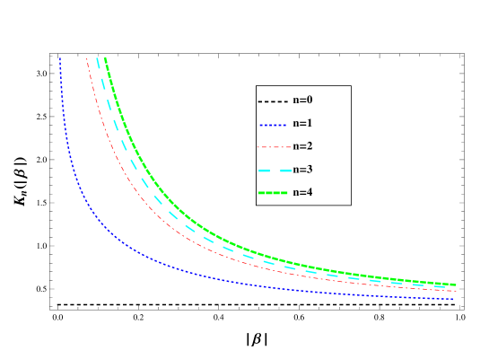
Figure 1: Plots of the non-oscillating and positive definite measures ${K}_{\textbf{n}}(|\beta|)$ in terms of $|\beta|$ for different values of $\mathbf{n}$. The dotted and horizontal curve corresponds to the Glauber two-variable minimum uncertainty coherent states $|\beta,\alpha\rangle$.

This leads to the following resolution of unity via bounded, positive definite and non-oscillating measures, $d\eta_{\mathbf{n}}(|\beta|):=K_{\mathbf{n}}(|\beta|)\frac{d|\beta|^{2}}{2}d\varphi$, in terms of the Meijer’s G-function( see $\frac{7-811}{4}$ in [13])

$$\oint_{\mathbb{C}(\beta)}{|\beta,\alpha;\mathbf{n}\rangle\hskip 2.84526pt\langle\beta,\alpha;\mathbf{n}|}d\eta_{\mathbf{n}}(|\beta|)=I_{\mathbf{n}},$$ (25)

$${K}_{\mathbf{n}}(|\beta|)=\frac{\mathbf{n}!}{\pi}e^{|\beta|^{2}}L_{\mathbf{n}}\left(-|\beta|^{2}\right)G\left([[\hskip 2.84526pt],[\mathbf{n}]],[[0,0],[\hskip 2.84526pt]],|\beta|^{2}\right).$$ (26)

We have plotted the changes of the function ${K}_{\mathbf{n}}(|\beta|)$ in Figure 1.

3.3 Time Evolution

As we discussed above, displaced number states $\left|\alpha\right\rangle_{n}^{b}$ form complete set of orthonormal states which satisfy an eigenvalue equation

$$H\left|\alpha\right\rangle_{n}^{b}=\hbar\omega\left(n+\frac{1}{2}\right)\left|\alpha\right\rangle_{n}^{b}.$$ (27)

Then, by acting the time evolution operator on the states (19) it evolves in time as

$$e^{-i\frac{t}{\hbar}H}|\beta,\alpha;{\mathbf{n}}\rangle=\frac{e^{-\frac{|\beta|^{2}}{2}-i(\mathbf{n}+\frac{1}{2})\omega t}}{\sqrt{\mathbf{n}!L_{\mathbf{n}}\left(-|\beta|^{2}\right)}}\sum^{\infty}_{n=0}{\left(\beta e^{-i\omega t}\right)^{n}\sqrt{\frac{({\mathbf{n}}+n)!}{n!^{2}}}|\alpha\rangle^{b}_{n+{\mathbf{n}}}}$$

$$\hskip 34.1433pt=e^{-i(\mathbf{n}+\frac{1}{2})\omega t}|\beta e^{-i\omega t},\alpha;{\mathbf{n}}\rangle,$$ (28)

the temporal stability follows easily, which illustrates the fact that the time evolution of such states remain within the family of coherent states.

3.4 Construction of Nonlinearity function

In this section we construct the explicit form of the operator valued of nonlinearity function associated to these new photon added coherent states. Since, the coherent states $|\beta,\alpha\rangle$ satisfy the following eigenvalue equation

$$a|\beta,\alpha\rangle=\beta|\beta,\alpha\rangle,$$

so, multiplying both sides of this equation by $\left(a^{{\dagger}}\right)^{\mathbf{n}}$ yields

$$\left(a^{{\dagger}}\right)^{\mathbf{n}}a|\beta,\alpha\rangle=\beta\left(a^{{\dagger}}\right)^{\mathbf{n}}|\beta,\alpha\rangle.$$

Which, making use of the commutation relations $[a,a^{{\dagger}}]=1$ and the identities

$$\left(a^{{\dagger}}\right)^{\mathbf{n}}a=a\left(a^{{\dagger}}\right)^{\mathbf{n}}-\mathbf{n}\left(a^{{\dagger}}\right)^{\mathbf{n}-1},$$

it leads to

$$\left(1-\frac{\mathbf{n}}{a^{{\dagger}}a+1}\right)a|\beta,\alpha;\mathbf{n}\rangle=\beta|\beta,\alpha;\mathbf{n}\rangle,$$ (29)

and pretends them as nonlinear coherent states by the expression for nonlinearity function, in terms of the number operator ${N}(=a^{{\dagger}}a)$, as

$$1-\frac{\mathbf{n}}{N+1}.$$ (30)

Obviously, it transforms to the identity operator for $\mathbf{n}=0$.

3.5 Photon Number Distribution

Another aspect of these states is revealed by considering their photon number distribution $p^{\mathbf{n}}_{n,m}(\beta,\alpha)$, which is the probability of finding an oscillator described by the coherent state $|\beta,\alpha;\mathbf{n}\rangle$ in its $(n,m)^{th}$ state

$$p^{\mathbf{n}}_{n,m}(\beta,\alpha)=\frac{n!}{\mathbf{n}!(n+m)!(n-\mathbf{n})!^{2}}\frac{|\alpha|^{2(n+m)}|\beta|^{2(n-\mathbf{n})}}{L_{\mathbf{n}}\left(-|\beta|^{2}\right)}e^{-|\alpha|^{2}-|\beta|^{2}}$$

$$=\left[\frac{n!}{\mathbf{n}!(n-\mathbf{n})!L_{\mathbf{n}}\left(-|\beta|^{2}\right)}\frac{|\beta|^{2(n-\mathbf{n})}e^{-|\beta|^{2}}}{(n-\mathbf{n})!}\right]\left[\frac{|\alpha|^{2(n+m)}}{(n+m)!}e^{-|\alpha|^{2}}\right],\hskip 14.22636ptn\geq\mathbf{n}.$$ (31)

Clearly, depends on the choice of the parameters, we will see different features from Poissonian to no-Poissonian distribution. In fact, the dependence of the function $p^{\mathbf{n}}_{n,m}(\beta,\alpha)$ on the parameters $\mathbf{n},n,m$ and $\beta,\alpha$ provides more options in order to determine and especially control of the expected distribution. In a few cases the further analysis will focus on the latter issue.

$\diamondsuit$ Case $\mathbf{n}=0$:
Because of the fact that the Eq. (19) dealing with the well known Glauber two variable coherent states $|\beta,\alpha\rangle$ for $\mathbf{n}=0$ and it can be considered as the states describe two coupled simple harmonic oscillators, too. So, the probability of finding the state $|\beta,\alpha;\mathbf{n}=0\rangle$ in its $(n,m)^{th}$ states follow Poissonian regime, as we expected, i.e.

$$p^{0}_{n,m}(\beta,\alpha)=\left[\frac{|\beta|^{2n}e^{-|\beta|^{2}}}{n!}\right]\left[\frac{|\alpha|^{2(n+m)}}{(n+m)!}e^{-|\alpha|^{2}}\right].$$ (32)

$\diamondsuit$ Case $n=0$ (Lowest Landau Level):
It is really interesting to note that, the probability of finding the system in its lowest state obeys Poissonian distribution, i.e.

$$p^{\mathbf{n}}_{0,m}(\beta,\alpha)=e^{-|\beta|^{2}}\left[\frac{|\alpha|^{2m}}{m!}e^{-|\alpha|^{2}}\right]$$ (33)

$\diamondsuit$ Case $\mathbf{n}=n$:
Using the Eq. (31):

$$p^{\mathbf{n}=n}_{n,m}(\beta,\alpha)=\left[\frac{e^{-|\beta|^{2}}}{L_{{n}}\left(-|\beta|^{2}\right)}\right]\left[\frac{|\alpha|^{2(n+m)}}{(n+m)!}e^{-|\alpha|^{2}}\right],$$ (34)

it indicates that the system carrier a no-Poissonian distribution , except for $|\beta|=0$.

$\diamondsuit$ Case $n+m=0$ (Landau levels with lowest $z$-angular momentum):
Another situation is related to the case $n+m=0$, when the above mentioned system is in Landau levels with lowest $z$-angular momentum. Our calculations show that it experiences a no-Poissonian, i.e.

$$p^{\mathbf{n}}_{n,-n}(\beta,\alpha)=e^{-|\alpha|^{2}}\left[\frac{n!}{\mathbf{n}!(n-\mathbf{n})!L_{\mathbf{n}}\left(-|\beta|^{2}\right)}\frac{|\beta|^{2(n-\mathbf{n})}e^{-|\beta|^{2}}}{(n-\mathbf{n})!}\right]$$ (35)

3.5.1 Sub-Poissonian Statistics For The Field In PACSs

As we know, a measure of the variance of the photon number distribution is given by Mandel’s $Q_{\mathbf{n}}(|\beta|)$ parameter [14]

$$Q_{\mathbf{n}}(|\beta|)=\frac{\langle{{N}}^{2}\rangle_{\mathbf{n}}-{\langle{{N}\rangle}_{\mathbf{n}}}^{2}}{{\langle{{N}\rangle}_{\mathbf{n}}}}-1,$$ (36)

it provides a convenient way of studying the nonclassical properties of the field. For this reason we begin to calculate the expectation values of the number operator ${N}$ and it’s square in the basis of the PACSs

$${\langle{{N}\rangle}_{\mathbf{n}}}=(\mathbf{n}+1)\frac{L_{\mathbf{n}+1}(-|\beta|^{2})}{L_{\mathbf{n}}(-|\beta|^{2})}-1,$$

$$\langle{{N}}^{2}\rangle_{\mathbf{n}}=(\mathbf{n}+1)(\mathbf{n}+2)\frac{L_{\mathbf{n}+2}(-|\beta|^{2})}{L_{\mathbf{n}}(-|\beta|^{2})}-3(\mathbf{n}+1)\frac{L_{\mathbf{n}+1}(-|\beta|^{2})}{L_{\mathbf{n}}(-|\beta|^{2})}+1,$$

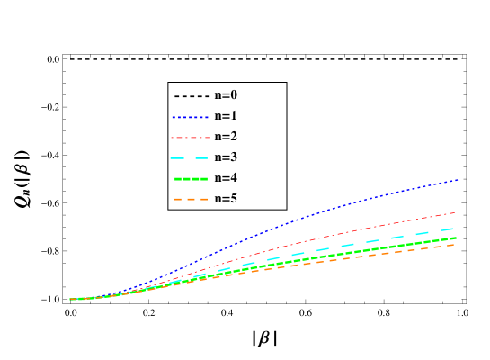
Figure 2: Mandel’s parameters ${Q}_{\mathbf{n}}(|\beta|)$ in the PACSs, versus $|\beta|$ for different values of $\mathbf{n}$. The dotted and horizontal curve $\left({Q}_{\mathbf{n}=0}(|\beta|)=0\right)$ corresponds to the standard Glauber coherent states.

Because of the structure of this function as illustrated in Figure 2, the states $|\beta,\alpha;\mathbf{n}\rangle$ show sub-Poissonian statistics( or fully anti-bunching effects).

3.6 Minimum Uncertainty Condition

Similar to what we have shown in our recent work [11], here we are looking for design ideas in the states $|\beta,\alpha;\mathbf{n}\rangle$. From these, the uncertainty condition for the field quadrature operators $x$ and it’s conjugate momenta $p_{x}$

$$x=\sqrt{\frac{\hbar}{2M\omega}}\left(b+b^{{\dagger}}-a-a^{{\dagger}}\right),\hskip 11.38109ptp_{x}=\frac{i}{2}\sqrt{\frac{M\hbar\omega}{2}}(b^{{\dagger}}-b+a-a^{{\dagger}}),$$ (37)

follow

$$\Delta:={\sigma^{(\mathbf{n})}_{xx}}{\sigma^{(\mathbf{n})}_{p_{x}p_{x}}}-{\sigma^{(\mathbf{n})}_{xp_{x}}}^{2},$$ (38)

where ${\sigma^{(\mathbf{n})}_{xx^{\prime}}}\left(=\frac{1}{2}\langle{xx^{\prime}+xx^{\prime}}\rangle_{\mathbf{n}}-\langle x\rangle_{\mathbf{n}}\langle x^{\prime}\rangle_{\mathbf{n}}\right)$ and the angular brackets denote averaging over PACSs for which the mean values are well defined, i.e.

$$\langle x\rangle_{\mathbf{n}}={\langle\beta,\alpha;\mathbf{n}|}x|\beta,\alpha;\mathbf{n}\rangle.$$

For instance, we have the following expectation values

$$\left\langle b\right\rangle_{\mathbf{n}}=\overline{\left\langle b^{{\dagger}}\right\rangle}_{\mathbf{n}}=\alpha,$$

$$\left\langle b^{2}\right\rangle_{\mathbf{n}}=\overline{\left\langle\left(b^{{\dagger}}\right)^{2}\right\rangle}_{\mathbf{n}}=\alpha^{2},$$

$$\left\langle b^{{\dagger}}b\right\rangle_{\mathbf{n}}=\overline{\left\langle bb^{{\dagger}}\right\rangle}_{\mathbf{n}}-1=|\alpha|^{2},$$

$$\left\langle a\right\rangle_{\mathbf{n}}=\overline{\left\langle a^{{\dagger}}\right\rangle}_{\mathbf{n}}=\frac{L^{1}_{\mathbf{n}}\left(-|\beta|^{2}\right)}{L_{\mathbf{n}}\left(-|\beta|^{2}\right)}\beta,$$

$$\left\langle a^{2}\right\rangle_{\mathbf{n}}=\overline{\left\langle\left({a^{{\dagger}}}\right)^{2}\right\rangle}_{\mathbf{n}}=\frac{L^{2}_{\mathbf{n}}\left(-|\beta|^{2}\right)}{L_{\mathbf{n}}\left(-|\beta|^{2}\right)}\beta^{2},$$

$$\left\langle a^{{\dagger}}a\right\rangle_{\mathbf{n}}=\left\langle aa^{{\dagger}}\right\rangle_{\mathbf{n}}-1=\left\langle N\right\rangle.$$

Where they result

$${\sigma^{(\mathbf{n})}_{xx}}=\frac{\hbar}{M\omega}\left[\frac{(\mathbf{n}+1)L_{\mathbf{n}+1}\left(-|\beta|^{2}\right)+|\beta|^{2}\cos(2\theta)L^{2}_{\mathbf{n}}\left(-|\beta|^{2}\right)-2|\beta|^{2}{\cos(\theta)}^{2}\frac{L^{1}_{\mathbf{n}}\left(-|\beta|^{2}\right)^{2}}{L_{\mathbf{n}}\left(-|\beta|^{2}\right)}}{L_{\mathbf{n}}\left(-|\beta|^{2}\right)}\right],$$ (39)

$${\sigma^{(\mathbf{n})}_{p_{x}p_{x}}}=\frac{M\hbar\omega}{4}\left[\frac{(\mathbf{n}+1)L_{\mathbf{n}+1}\left(-|\beta|^{2}\right)-|\beta|^{2}\cos(2\theta)L^{2}_{\mathbf{n}}\left(-|\beta|^{2}\right)-2|\beta|^{2}{\sin(\theta)}^{2}\frac{L^{1}_{\mathbf{n}}\left(-|\beta|^{2}\right)^{2}}{L_{\mathbf{n}}\left(-|\beta|^{2}\right)}}{L_{\mathbf{n}}\left(-|\beta|^{2}\right)}\right],$$ (40)

$${\sigma^{(\mathbf{n})}_{xp_{x}}}=\frac{\hbar}{2}|\beta|^{2}\sin(2\theta)\left[\frac{L^{2}_{\mathbf{n}}\left(-|\beta|^{2}\right)-\frac{L^{1}_{\mathbf{n}}\left(-|\beta|^{2}\right)^{2}}{L_{\mathbf{n}}\left(-|\beta|^{2}\right)}}{L_{\mathbf{n}}\left(-|\beta|^{2}\right)}\right].$$ (41)

Clearly the minimum uncertainty condition is violated, except for the values $\mathbf{n}=0$ or $|\beta|\gg 1$, which implies the existence of non-classical properties that will be investigated.

3.6.1 Squeezing Properties

Our final step is to reveal that measurements on the states $|\beta,\alpha;\mathbf{n}\rangle$ come with squeezing for the field quadrature operators $x$ and $p_{x}$. In accordance with Walls [15], a set of quantum states are called squeezed states if they have less uncertainty in one quadrature ($x$ or $p_{x}$) than coherent states. Using the relations (39) and (40), it is easy to see that ${\sigma^{(\mathbf{n})}_{xx}}$ and ${\sigma^{(\mathbf{n})}_{p_{x}p_{x}}}$ are dependent on the complex variable $\beta(=|\beta|e^{i\theta})$, the deformation parameter $\mathbf{n}$ and the variations of the cyclotron frequency $\omega$ which comes from the variations of magnetic field $B_{ext}$ and indicate that the squeezing properties could be varied by the changes of the external magnetic field. Our calculations show that these states exhibit squeezing in one of $x$ or $p_{x}$ quadratures, clearly in different domains. In Figure 3(a), we have presented ${\sigma^{(\mathbf{n})}_{p_{x}p_{x}}}$ against $|\beta|$ for $\theta=0$ and different values of $\mathbf{n}(=0,1,2,3,4,5)$. They become smaller than $\frac{1}{2}$ for sufficiently large $|\beta|$. Although for the values $\mathbf{n}=0,1$ we will see the fully squeezing in the whole range of $|\beta|$ and $\theta$, i.e.

$$\forall\hskip 2.84526pt|\beta|\in\mathbb{R}^{+},\forall\hskip 2.84526pt\theta\in[0,2\pi]\mid\hskip 5.69054pt{\sigma^{(\mathbf{n}=0,1)}_{p_{x}p_{x}}}<\frac{1}{2}.$$

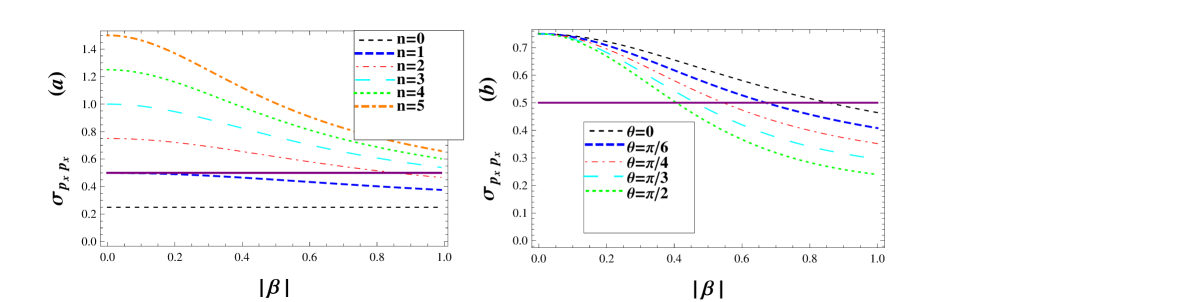
Figure 3: (a) Squeezing in the $p_{x}$ quadrature against $|\beta|$ for $\theta=0$ and different values of $\mathbf{n}=0,1,2,3,4,5$. (b) Squeezing in the $p_{x}$ quadrature against $|\beta|$ for different values of $\theta=0,\pi/6,\pi/4,\pi/3,\pi/2$ where we fixed $\textbf{n}=2$. The horizontal and solid line ${\sigma_{pp}}=\frac{1}{2}$, is correspond to the canonical coherent state.

Another situation depicting the variation of ${\sigma^{(m)}_{p_{x}p_{x}}}$ in terms of $|\beta|$ for different values of $\theta=0,\frac{\pi}{6},\frac{\pi}{4},\frac{\pi}{3},\frac{\pi}{2}$, while for fixed $\mathbf{n}=2$. Figure 3 (b) show that, by decreasing $|\beta|$, the degree of squeezing is enhanced, specially it passes the greatest value when $\theta$ reaches $\frac{\pi}{2}$. It is worth to mention that, this feature is not observed in the position coordinate $x$ for any value of the parameters $\beta$ and $\mathbf{n}$. It is important to note that we will see the fully squeezing in $|\beta,\alpha,\mathbf{n}=0\rangle$ [12]( the lowest horizontal line in the left part of Figure 3(a)), this mean that $\sigma_{p_{x}p_{x}}=\frac{M\hbar\omega}{4}<\frac{1}{2}$, while it minimize the minimum uncertainty condition too ( i.e. $\Delta=\sigma_{xx}\sigma_{p_{x}p_{x}}-\sigma_{xp_{x}}^{2}=\frac{\hbar^{2}}{4}$) [11]. In other word, in addition to the requirement to minimize the minimum uncertainty condition they carrier squeezing properties too, which is unique in its kind.

4 Theoretical Frameworks of Generation of the States $|\beta,\alpha\rangle$ and $|\beta,\alpha;\mathbf{n}\rangle$

Now, we propose theoretical frameworks to generate these states in practice. We first discuss the way of generating the two-variable coherent states, $|\beta,\alpha\rangle$. Then the way of producing the ”photon-added” states $|\beta,\alpha;\mathbf{n}\rangle$ relevant to the two-variable coherent states for the system has been reviewed in details.

4.1 Generation of the States $|\beta,\alpha\rangle$

We consider a Hamiltonian in which a two level atom interacts with two different modes of the cavity fields via an intensity-dependent coupling also an external classical field. Based on the rotating-wave approximation theory and the resonance condition, the Hamiltonian becomes the following form (assuming $\hbar=1)$:

$$H=g(\sigma_{-}e^{i\varphi}+\sigma_{+}e^{i\varphi})+\Omega_{1}(a^{\dagger}\sigma_{-}+a\sigma_{+})+\Omega_{1}(b^{\dagger}\sigma_{-}+b\sigma_{+})$$ (42)

where two different copies of the creation and annihilation operators $(a,a^{\dagger})$ and $(b,b^{\dagger})$, respectively, describe the two different modes of the cavity fields. The parameters $\Omega_{1},\Omega_{2}$ and $g$ are referred to the coupling coefficients of a two level atom with cavity and classical fields, where the latter include the phase $\varphi$. Also, the operators $\sigma_{-}=|g\rangle\langle e|$ and $\sigma_{+}=|e\rangle\langle g|$ denote the atomic lowering and raising operators, respectively, in terms of a two level atomic ground( $|g\rangle$) and exited( $|e\rangle$) states. Here, we assume that the coupling of the atom with the classical field be stronger than the coupling of the atom with the cavity fields, i.e. $(g\gg\Omega_{1},\Omega_{2})$.

Considering a situation in which the cavity is initially prepared in the vacuum of the fields and, also, the atom in a superposition of excited and ground states with equal weights:

$$\psi(0)=\left(\frac{|g\rangle+|e\rangle}{\sqrt{2}}\right)|0,0\rangle.$$ (43)

Along with the time evolution operator [16]

$$U(t)=R^{\dagger}T^{\dagger}(t)U_{eff}T(0)R,$$ (44)

where

$$R=e^{\frac{\pi}{4}(\sigma_{+}-\sigma_{-})}e^{\frac{i\varphi}{2}\sigma_{z}}=\frac{1}{\sqrt{2}}(\hat{I}+\sigma_{+}-\sigma_{-})e^{\frac{i\varphi}{2}\sigma_{z}},$$

$$T(t)=e^{ig\sigma_{z}t},$$

$$U_{eff}=e^{\frac{i\Omega_{1}t}{2}(a^{\dagger}e^{-i\varphi}+ae^{i\varphi})\sigma_{z}}e^{\frac{i\Omega_{2}t}{2}(b^{\dagger}e^{-i\varphi}+be^{i\varphi})\sigma_{z}}$$ (45)

, one can show that the system evolves into

$$\psi(t)=U(t)\psi(0)=R^{\dagger}T^{\dagger}(t)U_{eff}T(0)R\psi(0)$$

$$=R^{\dagger}T^{\dagger}(t)\left\{\cos\left(\frac{\varphi}{2}\right)e^{\frac{i\Omega_{1}t}{2}(a^{\dagger}e^{-i\varphi}+ae^{i\varphi})}\,e^{\frac{i\Omega_{2}t}{2}(b^{\dagger}e^{-i\varphi}+be^{i\varphi})}|0,0\rangle|e\rangle\right.$$

$$\hskip 34.1433pt\left.-i\sin\left(\frac{\varphi}{2}\right)\,e^{-\frac{i\Omega_{1}t}{2}(a^{\dagger}e^{-i\varphi}+ae^{i\varphi})}\,e^{-\frac{i\Omega_{2}t}{2}(b^{\dagger}e^{-i\varphi}+be^{i\varphi})}|0,0\rangle|g\rangle\right\}$$

$$=R^{\dagger}T^{\dagger}(t)\left\{\cos\left(\frac{\varphi}{2}\right)\,e^{\frac{i\Omega_{1}t}{2}(a^{\dagger}e^{-i\varphi}+ae^{i\varphi})}\left|\frac{-i\Omega_{2}t}{2}e^{-i\varphi}\right\rangle_{0}^{b}|e\rangle-i\sin\left(\frac{\varphi}{2}\right)\,e^{-\frac{i\Omega_{1}t}{2}(a^{\dagger}e^{-i\varphi}+ae^{i\varphi})}\left|\frac{i\Omega_{2}t}{2}e^{-i\varphi}\right\rangle_{0}^{b}|g\rangle\right\}$$

$$=R^{\dagger}T^{\dagger}(t)\left\{\cos\left(\frac{\varphi}{2}\right)\left|\frac{i\Omega_{1}t}{2}e^{-i\varphi},\frac{-i\Omega_{2}t}{2}e^{-i\varphi}\right\rangle|e\rangle-i\sin\left(\frac{\varphi}{2}\right)\left|\frac{-i\Omega_{1}t}{2}e^{-i\varphi},\frac{i\Omega_{2}t}{2}e^{-i\varphi}\right\rangle|g\rangle\right\}$$

$$=R^{\dagger}\left\{e^{-igt}\cos\left(\frac{\varphi}{2}\right)\,\left|\frac{i\Omega_{1}t}{2}e^{-i\varphi},\frac{-i\Omega_{2}t}{2}e^{-i\varphi}\right\rangle|e\rangle-ie^{igt}\sin\left(\frac{\varphi}{2}\right)\left|\frac{-i\Omega_{1}t}{2}e^{-i\varphi},\frac{i\Omega_{2}t}{2}e^{-i\varphi}\right\rangle|g\rangle\right\}$$

$$=\frac{1}{\sqrt{2}}\left\{e^{-i(gt+\frac{\varphi}{2})}\cos\left(\frac{\varphi}{2}\right)\,\left|\frac{i\Omega_{1}t}{2}e^{-i\varphi},\frac{-i\Omega_{2}t}{2}e^{-i\varphi}\right\rangle-ie^{i(gt+\frac{\varphi}{2})}\sin\left(\frac{\varphi}{2}\right)|\frac{-i\Omega_{1}t}{2}e^{-i\varphi},\frac{i\Omega_{2}t}{2}e^{-i\varphi}\rangle\right\}|g\rangle$$

$$+\frac{1}{\sqrt{2}}\left\{e^{-i(gt+\frac{\varphi}{2})}\cos\left(\frac{\varphi}{2}\right)\,\left|\frac{i\Omega_{1}t}{2}e^{-i\varphi},\frac{-i\Omega_{2}t}{2}e^{-i\varphi}\right\rangle+ie^{i(gt+\frac{\varphi}{2})}\sin\left(\frac{\varphi}{2}\right)\left|\frac{-i\Omega_{1}t}{2}e^{-i\varphi},\frac{i\Omega_{2}t}{2}e^{-i\varphi}\right\rangle\right\}|e\rangle.$$ (46)

By setting the parameters $\alpha:=-\frac{i\Omega_{2}t}{2}e^{-i\varphi}$ and $\beta:=\frac{i\Omega_{1}t}{2}e^{-i\varphi}$, the final state $|\psi(t)\rangle$ becomes a general superposition of two variable coherent states of Landau levels:

$$|\psi(t)\rangle=\frac{1}{\sqrt{2}}\left\{e^{-i(gt+\frac{\varphi}{2})}\cos\left(\frac{\varphi}{2}\right)\,|\beta,\alpha\rangle-ie^{i(gt+\frac{\varphi}{2})}\sin\left(\frac{\varphi}{2}\right)|-\beta,-\alpha\rangle\right\}|g\rangle$$

$$+\frac{1}{\sqrt{2}}\left\{e^{-i(gt+\frac{\varphi}{2})}\cos\left(\frac{\varphi}{2}\right)\,|\beta,\alpha\rangle+ie^{i(gt+\frac{\varphi}{2})}\sin\left(\frac{\varphi}{2}\right)|-\beta,-\alpha\rangle\right\}|e\rangle.$$ (47)

Then, depending on the state in which the atom is prepared, different situations of the quantized cavity fields can be obtained. For instance, if the atom is prepared in excited or ground state, the fields will become, respectively, into:

$$\psi_{g}(t)=N_{g}\left\{e^{-i\frac{\varphi}{2}}\cos\left(\frac{\varphi}{2}\right)\,|\beta,\alpha\rangle-ie^{i\frac{\varphi}{2}}\sin\left(\frac{\varphi}{2}\right)|-\beta,-\alpha\rangle\right\},$$

$$\psi_{e}(t)=N_{e}\left\{e^{-i\frac{\varphi}{2}}\cos\left(\frac{\varphi}{2}\right)\,|\beta,\alpha\rangle+ie^{i\frac{\varphi}{2}}\sin\left(\frac{\varphi}{2}\right)|-\beta,-\alpha\rangle\right\},$$ (48)

where we have used $N_{(g,e)}=\sqrt{2}$ and $gt=2k\pi$. Clearly, by choosing $\varphi=2\pi$ and $\pi$, regardless of the atomic detection, the state of the fields result the two variable coherent states $|\beta,\alpha\rangle$ and $|-\beta,-\alpha\rangle$ respectively.

4.2 Generation of the exited coherent states $|\beta,\alpha;\mathbf{n}\rangle$

At this stage we follow an approach that results the realization of the framework for the production of the excited states $|\beta,\alpha;\mathbf{n}\rangle$. These states can be produced by interaction of a two level atom with a two mode cavity field $|\beta,\alpha\rangle$, which can be described with the interaction Hamiltonian:

$$H_{int}=\hbar\mu\sigma_{+}a+h.c.$$ (49)

Assume that, we are preparing the initial state of the system as

$$|\Psi(t=0)\rangle=|\beta,\alpha\rangle|e\rangle,$$ (50)

then, in the next and small enough time we have

$$|\Psi(t)\rangle=e^{-\frac{it}{\hbar}H_{int}}|\beta,\alpha\rangle|e\rangle,$$

$$\hskip 25.60747pt\vdots$$

$$\hskip 22.76219pt\Downarrow$$

$$|\Psi(t)\rangle=|\beta,\alpha\rangle|e\rangle-{i\mu t}a^{{\dagger}}|\beta,\alpha\rangle|g\rangle.$$ (51)

Now, depending on the situation in which the atom is detected, the state of the two mode field may be determined. If the atom is detected in a ground state, the state of the field will be collapsed to $a^{{\dagger}}|\beta,\alpha\rangle$. Finally, extension the above arguments to multi photon process, the outcome photon field will be a state $\left(a^{{\dagger}}\right)^{n}|\beta,\alpha\rangle$, which are the new type of the excited ( or photon added) coherent states $|\beta,\alpha,\mathbf{n}\rangle$, were discussed above.

5 Discussion and Outline

Based on the action of the creation operator of the Weyl-Heisenberg algebra, broad range of states that are called two variable Agarwal’s type of PACSs are produced , for first time based on our knowledge. Realization of resolution of the identity condition, be obtained with respect to the non-oscillating and positive definite measure on the complex plane. Finally, non-classical properties of such states have been reviewed in detail. For instance, it has been shown that:
$\bullet$ Their squeezing properties, which could be varied not only by the magnitude of the external magnetic field $B_{ext}$, also by the quantum number $\mathbf{n}$ and by the complex variables $\beta$. This allows to the experimenter to adjust the appropriate parameters to control the quantities.
$\bullet$ They result that, squeezing properties in $p_{x}$ is efficiently considerable where $B_{ext}$ is decreased. However, we would not expect to take squeezing in $x$ component.
$\bullet$ One can show that $|\beta,\alpha,\mathbf{n}\rangle$ satisfies sub-Poissonian statistics, that is independent of the choice of the parameters.
$\bullet$ It is important to note that we will see the fully squeezing in $|\beta,\alpha,\mathbf{n}=1\rangle$ and $|\beta,\alpha,\mathbf{n}=0\rangle$, while the latter minimize the minimum uncertainty condition too.
$\bullet$ Finally it is worth to mention that the scheme proposed here to construct PACSs in terms of the Glauber two variable coherent states, could be applied to two other classes of minimum uncertainty coherent states which were introduced in [11].

Acknowledgments
This work has been supported by a grant/research fund from Azarbaijan Shahid Madani University.

References

• [1] G. S. Agarwal and K Tara ‘Nonclassical properties of states generated by the excitations on a coherent state’ Phys. Rev. A 43, 492 (1991).
• [2] A. Zavatta, S. Viciani and M. Bellini ‘Quantum-to-Classical Transition with Single-Photon-Added Coherent States of Light’ Science 306, 660 (2004).
• [3] V. V. Dodonov, M. A. Marchiolli, Ya. A. Korennoy, V. I. Man ko and Y. A. Moukhin‘Dynamical squeezing of photon-added coherent states’ Phys. Rev. A 58, 4087 (1998).
• [4] S. Sivakumar ‘Photon-added coherent states as nonlinear coherent states’ J. Phys. A: Math. Gen. 32, 3441 (1999).
• [5] A. Dehghani ‘General Displaced $SU(1,1)$ number states - revisitedAccepted for publication in J. Math. Phys (2014).
• [6] I. A. Malkin and V. I. Manko ‘Coherent states of a charged particle in a magnetic field Soviet. Phys. JETP 28, 527 (1969).
• [7] I. A. Malkin, V. I. Manko, and D. A. Trifonov ‘Coherent States and Transition Probabilities in a Time-Dependent Electromagnetic Field’ Phys. Rev. D 2, 1371 (1970).
• [8] I. A. Malkin, V. I. Man’ko, and D. A. Trifonov ‘Evolution of coherent states of a charged particle in a variable magnetic field Soviet. Phys. JETP 31, 386 (1970).
• [9] I. A. Malkin, V. I. Man’ko, and D. A. Trifonov ‘Linear adiabatic invariants and coherent states’ J. Math. Phys. 14, 576 (1973).
• [10] A. Feldman, A.H. Kahn ‘Landau diamagnetism from the coherent states of an electron in a uniform magnetic field’ Phys. Rev. B 1, 4584-4589 (1970).
• [11] A. Dehghani, H. Fakhri and B. Mojaveri ‘The minimum-uncertainty coherent states for Landau levels’ J. Math. Phys 53, 123527 (2012).
• [12] A. Dehghani and B. Mojaveri ‘New Physics in Landau Levels’ J. Phys. A J. Phys. A: Math. Theor 46 385303 (2013).
• [13] I. S. Gradshteyn and I. M. Ryzhik ‘Table of Integrals, Series, and Products’ (San Diego, CA: Academic) (2000)
• [14] L. Mandel ‘Sub-Poissonian photon statistics in resonance fluorescence’ Opt. Lett. 4, 205 (1979).
• [15] D. F. Walls ‘Squeezed states of light’ Nature 306, 141 (1983).
• [16] X. Zou, K. Pahlke and W. Mathis ‘Scheme for direct measurement of the Wigner characteristic function in cavity QED’ Phys. Rev. A 69, 015802 (2004).