11institutetext: E. Koblents and J. Míguez 22institutetext: Department of Signal Theory and Communications, Universidad Carlos III de Madrid, Madrid, Spain
22email: ekoblents,jmiguez@tsc.uc3m.es

A comparison of nonlinear population Monte Carlo and particle Markov chain Monte Carlo algorithms for Bayesian inference in stochastic kinetic models thanks: E. K. acknowledges the support of Ministerio de Educación of Spain (Programa de Formación de Profesorado Universitario, ref. AP2008-00469). This work has been partially supported by Ministerio de Economía y Competitividad of Spain (program Consolider-Ingenio 2010 CSD2008-00010 COMONSENS and project COMPREHENSION TEC2012-38883-C02-01).

Eugenia Koblents    Joaquín Míguez
(Received: date / Accepted: date)
Abstract

In this paper we address the problem of Monte Carlo approximation of posterior probability distributions in stochastic kinetic models (SKMs). SKMs are multivariate Markov jump processes that model the interactions among species in biochemical systems according to a set of uncertain parameters. Markov chain Monte Carlo (MCMC) methods have been typically preferred for this Bayesian inference problem. Specifically, the particle MCMC (pMCMC) method has been recently shown to be an effective, while computationally demanding, method applicable to this problem. Within the pMCMC framework, importance sampling (IS) has been used only as the basis of the sequential Monte Carlo (SMC) approximation of the acceptance ratio in the Metropolis-Hastings kernel. However, the recently proposed nonlinear population Monte Carlo (NPMC) algorithm, based on an iterative IS scheme, has also been shown to be effective as a Bayesian inference tool for low dimensional (predator-prey) SKMs. In this paper, we provide an extensive performance comparison of pMCMC versus NPMC, when applied to the challenging prokaryotic autoregulatory network. We show how the NPMC method can greatly outperform the pMCMC algorithm in this scenario, with an overall moderate computational effort. We complement the numerical comparison of the two techniques with an asymptotic convergence analysis of the nonlinear IS scheme at the core of the proposed method when the importance weights can only be computed approximately.

Keywords:
Nonlinear population Monte Carlo particle Markov chain Monte Carlo sequential Monte Carlo stochastic kinetic models

1 Introduction

Stochastic kinetic models (SKMs) are multivariate systems that model molecular interactions among species in biological and chemical problems, according to a set of unknown rate parameters (Wilkinson, 2011b). The aim of this paper is the approximation of the posterior distribution of the rate parameters and the populations of all species, provided a set of discrete, noisy observations is available. This inference problem has been traditionally addressed using Markov chain Monte Carlo (MCMC) schemes (Boys et al, 2008; Milner et al, 2013; Wilkinson, 2011a, b). In (Golightly and Wilkinson, 2011) a particle MCMC (pMCMC) method (Andrieu et al, 2010) has been successfully applied to this problem. The pMCMC technique relies on a sequential Monte Carlo (SMC) approximation of the posterior distribution of the populations to compute the Metropolis-Hastings (MH) acceptance ratio.

However, MCMC methods in general, and pMCMC in particular, suffer from a number of problems. The convergence of the Markov chain is hard to assess and the final set of samples presents correlations which can greatly reduce its efficiency. Besides, MCMC methods do not (easily) allow for parallel implementations and turn out to be computationally intensive. To reduce the complexity of the existing MCMC methods when applied to SKMs, a diffusion approximation of the underlying stochastic process is usually applied (Golightly and Wilkinson, 2005). The parameters of the MCMC proposal are also hard to choose and determine the performance of the algorithm.

An appealing alternative to the widely established MCMC methods is the population Monte Carlo (PMC) algorithm (Cappé et al, 2004). PMC is an iterative importance sampling (IS) scheme that yields a discrete approximation of a target probability distribution. The PMC algorithm has important advantages with respect to MCMC techniques. It provides independent samples and asymptotically unbiased estimates at all iterations, which avoids the need of a convergence period. Additionally, PMC may be easily parallelized.

On the other hand, the main weakness of IS and PMC is their low efficiency in high dimensional problems, due to the well known degeneracy problem (Bengtsson et al, 2008). The recently proposed nonlinear PMC (NPMC) scheme (Koblents and Míguez, 2013b) mitigates this difficulty by computing nonlinear transformations of the importance weights (IWs), in order to smooth their variations and avoid degeneracy. In (Koblents and Míguez, 2013b) a simple convergence analysis of nonlinear IS (NIS) is provided, for two types of nonlinear transformations, tempering and clipping. Similarly to the pMCMC method in (Golightly and Wilkinson, 2011), the NPMC method resorts to an SMC approximation of the posterior distribution of the populations to compute, in our case, the IWs.

In (Koblents and Míguez, 2013a, c) the nonlinear version of IS and PMC is combined with the popular mixture-PMC (MPMC) method of (Cappé et al, 2008), which allows to approximate arbitrary high-dimensional target distributions by means of mixtures of Gaussian or t-Student distributions. The original MPMC algorithm of (Cappé et al, 2008) has been applied to cosmological inference problems and compared to an MCMC method in (Wraith, 2009) (and (Kilbinger, 2010)), and has been shown to provide similar precision results with a lower computation load than its MCMC counterpart. The MPMC scheme is the basis of the tool CosmoPMC (Kilbinger, 2012) for the estimation of cosmological parameters, as an alternative to the MCMC package, CosmoMC, (Lewis and Bridle, 2002) http://cosmologist.info/cosmomc.

In this paper we apply the NPMC method to the estimation of both the parameters and the unobserved populations in SKMs. We present numerical results to compare the performance of the state-of-art pMCMC and the proposed NPMC, when applied to the challenging prokaryotic model in two scenarios of different dimension and with two different observation models. We show that the NPMC method outperforms the pMCMC method for the same computational cost.

As a complement to the numerical comparison, we introduce new asymptotic convergence results for the NIS scheme that accounts for the use of SMC to approximate the IWs. The analysis in this paper considerably extends the preliminary results in (Koblents and Míguez, 2013b). In particular, we prove that approximate integrals computed via NIS converge almost surely (as the number of samples increases) and explicit convergence rates are given.

The rest of the paper is organized as follows. In Section 2 we present an introduction to the basics of SKMs and the usual solutions to this Bayesian inference problem. In Sections 3 and 4 we describe the pMCMC and NPMC methods, respectively, when applied to the approximation of posterior distributions in SKMs. In Section 5 we numerically compare the performance of pMCMC and NPMC schemes when applied to a prokaryotic autoregulatory model, with different simulation settings. Section 6 is devoted to the convergence analysis of the NIS method. Finally, Section 7 is devoted to the conclusions.

2 Bayesian inference for stochastic kinetic models

2.1 Stochastic kinetic models

A SKM is a multivariate continuous-time jump process modeling the interactions among molecules, or species, that take place in chemical reaction networks of biochemical and cellular systems (Wilkinson, 2011b).

Consider a biochemical reaction network that describes the time evolution of the population of V𝑉V species x1,,xVsubscript𝑥1subscript𝑥𝑉x_{1},\ldots,x_{V} related by means of K𝐾K reactions r1,,rKsubscript𝑟1subscript𝑟𝐾r_{1},\ldots,r_{K}

r1:p11x1+p12x2++p1VxVc1q11x1+q12x2++q1VxV,r2:p21x1+p22x2++p2VxVc2q21x1+q22x2++q2VxV,rK:pK1x1+pK2x2++pKVxVcKqK1x1+qK2x2++qKVxV,:subscript𝑟1absentsuperscriptsubscript𝑐1subscript𝑝11subscript𝑥1subscript𝑝12subscript𝑥2subscript𝑝1𝑉subscript𝑥𝑉absentmissing-subexpressionsubscript𝑞11subscript𝑥1subscript𝑞12subscript𝑥2subscript𝑞1𝑉subscript𝑥𝑉:subscript𝑟2absentsuperscriptsubscript𝑐2subscript𝑝21subscript𝑥1subscript𝑝22subscript𝑥2subscript𝑝2𝑉subscript𝑥𝑉absentmissing-subexpressionsubscript𝑞21subscript𝑥1subscript𝑞22subscript𝑥2subscript𝑞2𝑉subscript𝑥𝑉:subscript𝑟𝐾absentsuperscriptsubscript𝑐𝐾subscript𝑝𝐾1subscript𝑥1subscript𝑝𝐾2subscript𝑥2subscript𝑝𝐾𝑉subscript𝑥𝑉absentmissing-subexpressionsubscript𝑞𝐾1subscript𝑥1subscript𝑞𝐾2subscript𝑥2subscript𝑞𝐾𝑉subscript𝑥𝑉\displaystyle\begin{array}[]{cc}r_{1}:&p_{11}x_{1}+p_{12}x_{2}+\ldots+p_{1V}x_{V}\stackrel{{\scriptstyle c_{1}}}{{\longrightarrow}}\\ &q_{11}x_{1}+q_{12}x_{2}+\ldots+q_{1V}x_{V},\\ r_{2}:&p_{21}x_{1}+p_{22}x_{2}+\ldots+p_{2V}x_{V}\stackrel{{\scriptstyle c_{2}}}{{\longrightarrow}}\\ &q_{21}x_{1}+q_{22}x_{2}+\ldots+q_{2V}x_{V},\\ \vdots&\vdots\\ r_{K}:&p_{K1}x_{1}+p_{K2}x_{2}+\ldots+p_{KV}x_{V}\stackrel{{\scriptstyle c_{K}}}{{\longrightarrow}}\\ &q_{K1}x_{1}+q_{K2}x_{2}+\ldots+q_{KV}x_{V},\\ \end{array}

where pkvsubscript𝑝𝑘𝑣p_{kv} and qkvsubscript𝑞𝑘𝑣q_{kv}, k=1,,K𝑘1𝐾k=1,\ldots,K, v=1,,V𝑣1𝑉v=1,\ldots,V, denote the reactant and the product coefficients, respectively; and ck>0subscript𝑐𝑘0c_{k}>0, k=1,,K𝑘1𝐾k=1,\ldots,K, are the random constant rate parameters. A matrix P of size K×V𝐾𝑉K\times V contains the reactant coefficients pkvsubscript𝑝𝑘𝑣p_{kv} and, similarly, Q contains the product coefficients qkvsubscript𝑞𝑘𝑣q_{kv}. The stoichiometry matrix of size V×K𝑉𝐾V\times K is defined as S=(QP)SsuperscriptQPtop\textbf{S}=(\textbf{Q}-\textbf{P})^{\top}. The vector c=[c1,,cK]csuperscriptsubscript𝑐1subscript𝑐𝐾top\textbf{c}=[c_{1},\ldots,c_{K}]^{\top} contains the rate parameters.

Let xv(t)subscript𝑥𝑣𝑡x_{v}(t), v=1,,V𝑣1𝑉v=1,\ldots,V, denote the nonnegative, integer population of species xvsubscript𝑥𝑣x_{v} at time t𝑡t, and let x(t)=[x1(t),,xV(t)]x𝑡superscriptsubscript𝑥1𝑡subscript𝑥𝑉𝑡top\textbf{x}(t)=[x_{1}(t),\ldots,x_{V}(t)]^{\top} denote the state of the system at this time instant. Let xn=[x1,n,,xV,n]subscriptx𝑛superscriptsubscript𝑥1𝑛subscript𝑥𝑉𝑛top\textbf{x}_{n}=[x_{1,n},\ldots,x_{V,n}]^{\top} denote the state of the system at discrete time instants t=nΔ𝑡𝑛Δt=n\Delta, n=1,,N𝑛1𝑁n=1,\ldots,N, i.e., xv,n=xv(nΔ)subscript𝑥𝑣𝑛subscript𝑥𝑣𝑛Δx_{v,n}=x_{v}(n\Delta) where ΔΔ\Delta denotes a time-discretization period. We denote by x the VN×1𝑉𝑁1VN\times 1 vector containing the population of each species at N𝑁N consecutive discrete time instants, i.e., x=[x1,,xN]xsuperscriptsuperscriptsubscriptx1topsuperscriptsubscriptx𝑁toptop\textbf{x}=[\textbf{x}_{1}^{\top},\ldots,\textbf{x}_{N}^{\top}]^{\top}.

The k𝑘k-th reaction takes place stochastically according to its instantaneous rate or hazard function

hk(t)=ckv=1V(xv(t)pkv),k=1,,K,formulae-sequencesubscript𝑘𝑡subscript𝑐𝑘superscriptsubscriptproduct𝑣1𝑉binomialsubscript𝑥𝑣𝑡subscript𝑝𝑘𝑣𝑘1𝐾h_{k}(t)=c_{k}\prod_{v=1}^{V}{x_{v}(t)\choose p_{kv}},\quad k=1,\ldots,K,

where the product of binomial coefficients represents the number of combinations in which the k𝑘k-th reaction can occur, as a function of the population of each reactant species xvsubscript𝑥𝑣x_{v}. We additionally define the vector h(t)=[h1(t),,hK(t)]h𝑡superscriptsubscript1𝑡subscript𝐾𝑡top\textbf{h}(t)=[h_{1}(t),\ldots,h_{K}(t)]^{\top}. The waiting time to the next reaction is exponentially distributed with parameter h0(t)=k=1Khk(t)subscript0𝑡superscriptsubscript𝑘1𝐾subscript𝑘𝑡h_{0}(t)=\sum_{k=1}^{K}h_{k}(t), and the probability of each reaction type is given by hk(t)/h0(t)subscript𝑘𝑡subscript0𝑡h_{k}(t)/h_{0}(t).

2.2 Bayesian inference for SKMs

We consider the log-transformed rate parameters 𝜽=[θ1,,θK]𝜽superscriptsubscript𝜃1subscript𝜃𝐾top{\boldsymbol{\theta}}=[\theta_{1},\ldots,\theta_{K}]^{\top}, where θk=log(ck)subscript𝜃𝑘subscript𝑐𝑘\theta_{k}=\log(c_{k}), k=1,,K𝑘1𝐾k=1,\ldots,K, with prior pdf p(𝜽)𝑝𝜽p({\boldsymbol{\theta}}). The prior pdf of the initial population vector x0subscriptx0\textbf{x}_{0} is denoted by p(x0)𝑝subscriptx0p(\textbf{x}_{0}). We assume that a linear combination of the populations of a subset of species is observed at discrete time instants corrupted by Gaussian noise, i.e.,

yn=Mxn+wn,n=1,,N,formulae-sequencesubscripty𝑛subscriptMx𝑛subscriptw𝑛𝑛1𝑁\textbf{y}_{n}=\textbf{M}\textbf{x}_{n}+\textbf{w}_{n},\quad n=1,\ldots,N, (2)

where M is the observation matrix with dimensions D×V𝐷𝑉D\times V and wn𝒩D(wn;0,σ2I)similar-tosubscriptw𝑛subscript𝒩𝐷subscriptw𝑛0superscript𝜎2I\textbf{w}_{n}\sim\mathcal{N}_{D}(\textbf{w}_{n};\textbf{0},\sigma^{2}\textbf{I}) is a multivariate Gaussian noise component. We denote the complete observation vector with dimension DN×1𝐷𝑁1DN\times 1 as y=[y1,,yN]ysuperscriptsuperscriptsubscripty1topsuperscriptsubscripty𝑁toptop\textbf{y}=[\textbf{y}_{1}^{\top},\ldots,\textbf{y}_{N}^{\top}]^{\top}.

The dynamical behavior of an arbitrary SKM may be described in terms of the following set of equations111For simplicity of notation, in this section we use p𝑝p to denote the pdfs in the model. We write conditional pdfs as p(y|x)𝑝conditionalyxp(\textbf{y}|\textbf{x}), and joint densities as p(𝜽)=p(θ1,,θK)𝑝𝜽𝑝subscript𝜃1subscript𝜃𝐾p({\boldsymbol{\theta}})=p(\theta_{1},\ldots,\theta_{K}). This is an argument-wise notation, hence p(θ1)𝑝subscript𝜃1p(\theta_{1}) denotes the distribution of θ1subscript𝜃1\theta_{1}, possibly different from p(θ2)𝑝subscript𝜃2p(\theta_{2}).

{𝜽p(𝜽)(parameters prior),x0p(x0)(populations prior),xnp(xn|xn1,𝜽)(transition equation),ynp(yn|xn)(observation equation),casessimilar-to𝜽𝑝𝜽(parameters prior)similar-tosubscriptx0𝑝subscriptx0(populations prior)similar-tosubscriptx𝑛𝑝conditionalsubscriptx𝑛subscriptx𝑛1𝜽(transition equation)similar-tosubscripty𝑛𝑝conditionalsubscripty𝑛subscriptx𝑛(observation equation),\left\{\begin{array}[]{ll}{\boldsymbol{\theta}}\sim p({\boldsymbol{\theta}})&\quad\textrm{(parameters prior)},\\ \textbf{x}_{0}\sim p(\textbf{x}_{0})&\quad\textrm{(populations prior)},\\ \textbf{x}_{n}\sim p(\textbf{x}_{n}|\textbf{x}_{n-1},{\boldsymbol{\theta}})&\quad\textrm{(transition equation)},\\ \textbf{y}_{n}\sim p(\textbf{y}_{n}|\textbf{x}_{n})&\quad\textrm{(observation equation),}\end{array}\right.

where p(xn|xn1,𝜽)𝑝conditionalsubscriptx𝑛subscriptx𝑛1𝜽p(\textbf{x}_{n}|\textbf{x}_{n-1},{\boldsymbol{\theta}}) and p(yn|xn)𝑝conditionalsubscripty𝑛subscriptx𝑛p(\textbf{y}_{n}|\textbf{x}_{n}) denote the transition pdf and the likelihood function, respectively. The Gillespie algorithm (Gillespie, 1977) allows to perform exact forward simulations of arbitrary SKMs, drawing samples from the transition densities p(xn|xn1,𝜽)𝑝conditionalsubscriptx𝑛subscriptx𝑛1𝜽p(\textbf{x}_{n}|\textbf{x}_{n-1},{\boldsymbol{\theta}}), n=1,,N𝑛1𝑁n=1,\ldots,N, given a set of log-rate parameters 𝜽𝜽{\boldsymbol{\theta}} and an initial population x0subscriptx0\textbf{x}_{0}.

In this paper, we aim to obtain a Monte Carlo approximation of the full joint posterior distribution of the log-rate parameters 𝜽𝜽{\boldsymbol{\theta}} and the populations x, with density

p(𝜽,x|y)p(y|x)p(x|x0,𝜽)p(x0)p(𝜽),proportional-to𝑝𝜽conditionalxy𝑝conditionalyx𝑝conditionalxsubscriptx0𝜽𝑝subscriptx0𝑝𝜽p({\boldsymbol{\theta}},\textbf{x}|\textbf{y})\propto p(\textbf{y}|\textbf{x})p(\textbf{x}|\textbf{x}_{0},{\boldsymbol{\theta}})p(\textbf{x}_{0})p({\boldsymbol{\theta}}), (3)

given the prior distributions p(𝜽)𝑝𝜽p({\boldsymbol{\theta}}) and p(x0)𝑝subscriptx0p(\textbf{x}_{0}), the transition pdf p(x|x0,𝜽)=n=1Np(xn|xn1,𝜽)𝑝conditionalxsubscriptx0𝜽superscriptsubscriptproduct𝑛1𝑁𝑝conditionalsubscriptx𝑛subscriptx𝑛1𝜽p(\textbf{x}|\textbf{x}_{0},{\boldsymbol{\theta}})=\prod_{n=1}^{N}p(\textbf{x}_{n}|\textbf{x}_{n-1},{\boldsymbol{\theta}}) and the likelihood function p(y|x)=n=1Np(yn|xn)𝑝conditionalyxsuperscriptsubscriptproduct𝑛1𝑁𝑝conditionalsubscripty𝑛subscriptx𝑛p(\textbf{y}|\textbf{x})=\prod_{n=1}^{N}p(\textbf{y}_{n}|\textbf{x}_{n}) constructed from equation (2).

We are also interested in computing approximations of the posterior marginals of the rate parameters p(𝜽|y)=p(𝜽,x|y)𝑑x𝑝conditional𝜽y𝑝𝜽conditionalxydifferential-dxp({\boldsymbol{\theta}}|\textbf{y})=\int p({\boldsymbol{\theta}},\textbf{x}|\textbf{y})d\textbf{x} and the species populations p(x|y)=p(𝜽,x|y)𝑑𝜽𝑝conditionalxy𝑝𝜽conditionalxydifferential-d𝜽p(\textbf{x}|\textbf{y})=\int p({\boldsymbol{\theta}},\textbf{x}|\textbf{y})d{\boldsymbol{\theta}} as well as their moments (e.g., the posterior mean), which are of the form

Ep(𝜽|y)[f(𝜽)]=f(𝜽)p(𝜽|y)𝑑𝜽,andsubscript𝐸𝑝conditional𝜽ydelimited-[]𝑓𝜽𝑓𝜽𝑝conditional𝜽ydifferential-d𝜽andE_{p({\boldsymbol{\theta}}|\textbf{y})}[f({\boldsymbol{\theta}})]=\int f({\boldsymbol{\theta}})p({\boldsymbol{\theta}}|\textbf{y})d{\boldsymbol{\theta}},\;\textrm{and}
Ep(x|y)[f(x)]=f(x)p(x|y)𝑑x,respectively,subscript𝐸𝑝conditionalxydelimited-[]𝑓x𝑓x𝑝conditionalxydifferential-dxrespectivelyE_{p(\textbf{x}|\textbf{y})}[f(\textbf{x})]=\int f(\textbf{x})p(\textbf{x}|\textbf{y})d\textbf{x},\;\textrm{respectively},

where f𝑓f is a real, integrable function.

Bayesian inference based on exact stochastic simulations from p(xn|xn1,𝜽)𝑝conditionalsubscriptx𝑛subscriptx𝑛1𝜽p(\textbf{x}_{n}|\textbf{x}_{n-1},{\boldsymbol{\theta}}) generated via the Gillespie algorithm often becomes practically intractable even for models of modest complexity (Golightly and Wilkinson, 2005). Thus, it is very common to resort to a continuous approximation of the underlying stochastic process, which is known as the diffusion approximation. The diffusion process that most closely matches the dynamics of the associated Markov jump process, over an infinitesimal time interval (t,t+dt]𝑡𝑡𝑑𝑡(t,t+dt], is given by a stochastic differential equation known as the chemical Langevin equation (CLE) (Wilkinson, 2011b) (pag 230)

dx(t)=Sh(t)dt+Sdiag{h(t)}Sdw(t),𝑑x𝑡Sh𝑡𝑑𝑡Sdiagh𝑡superscriptStop𝑑w𝑡d\textbf{x}(t)=\textbf{S}\,\textbf{h}(t)dt+\sqrt{\textbf{S}\,\textrm{diag}\{\textbf{h}(t)\}\textbf{S}^{\top}}d\textbf{w}(t),

driven by the V×1𝑉1V\times 1 dimensional Wiener process w(t)w𝑡\textbf{w}(t). However, this approximation is known to be poor in low concentration scenarios, and thus should be avoided for models involving species with a very low population. Alternatively, in (Milner et al, 2013) the authors propose a solution based on a moment closure approximation of the stochastic process.

This inference problem has been traditionally addressed using MCMC methods, and IS based schemes have been avoided due to their inefficiency in high dimensional spaces (Wilkinson, 2011b). In (Boys et al, 2008) various MCMC algorithms are evaluated in data-poor scenarios. In (Golightly and Wilkinson, 2011) a likelihood-free pMCMC scheme (Andrieu et al, 2010) is applied to this problem. This method is, to the best of our knowledge, the most powerful, yet computationally expensive, method provided so far for this kind of applications.

In (Koblents and Míguez, 2013b) a NPMC scheme is proposed for the approximation of the marginal posterior pdf p(𝜽|y)𝑝conditional𝜽yp({\boldsymbol{\theta}}|\textbf{y}), which is computationally competitive, since it requires the processing of a low number of samples of 𝜽𝜽{\boldsymbol{\theta}} to obtain the approximation of the posterior. The performance of the NPMC method is tested in a simple SKM known as predator-prey model (Volterra, 1926), providing excellent results with a low computational cost.

In this paper we compare the performances of the pMCMC and the NPMC methods in the approximation of the full joint posterior p(𝜽,x|y)𝑝𝜽conditionalxyp({\boldsymbol{\theta}},\textbf{x}|\textbf{y}) in equation (3), which allows to perform Bayesian inference for the rate parameters 𝜽𝜽{\boldsymbol{\theta}} and the full sample path x, including unobserved components.

3 Particle MCMC for SKMs

The particle marginal Metropolis-Hastings (PMMH) algorithm is a pMCMC method originally proposed in (Andrieu et al, 2010) for Monte Carlo sampling from the full posterior distribution p(𝜽,x|y)𝑝𝜽conditionalxyp({\boldsymbol{\theta}},\textbf{x}|\textbf{y}). The PMMH scheme suggests a proposal mechanism of the form q(𝜽|𝜽)p^J(x|y,𝜽)𝑞conditionalsuperscript𝜽𝜽superscript^𝑝𝐽conditionalsuperscriptxysuperscript𝜽q({\boldsymbol{\theta}}^{\star}|{\boldsymbol{\theta}})\hat{p}^{J}(\textbf{x}^{\star}|\textbf{y},{\boldsymbol{\theta}}^{\star}). A new candidate in the parameter space, 𝜽superscript𝜽{\boldsymbol{\theta}}^{\star}, is drawn from an arbitrary proposal distribution q(𝜽|𝜽)𝑞conditionalsuperscript𝜽𝜽q({\boldsymbol{\theta}}^{\star}|{\boldsymbol{\theta}}), while the new candidate in the variable space, xsuperscriptx\textbf{x}^{\star}, is generated using an approximation of the posterior marginal p(x|y,𝜽)𝑝conditionalsuperscriptxysuperscript𝜽p(\textbf{x}^{\star}|\textbf{y},{\boldsymbol{\theta}}^{\star}) constructed by means of an SMC algorithm (i.e., a particle filter) with J𝐽J particles and denoted p^J(x|y,𝜽)superscript^𝑝𝐽conditionalsuperscriptxysuperscript𝜽\hat{p}^{J}(\textbf{x}^{\star}|\textbf{y},{\boldsymbol{\theta}}^{\star}). The probability of accepting the proposed pair (𝜽,x)superscript𝜽superscriptx({\boldsymbol{\theta}}^{\star},\textbf{x}^{\star}) is

min{1,p^J(y|𝜽)p(𝜽)p^J(y|𝜽)p(𝜽)×q(𝜽|𝜽)q(𝜽|𝜽)},1superscript^𝑝𝐽conditionalysuperscript𝜽𝑝superscript𝜽superscript^𝑝𝐽conditionaly𝜽𝑝𝜽𝑞conditional𝜽superscript𝜽𝑞conditionalsuperscript𝜽𝜽\min\left\{1,\frac{\hat{p}^{J}(\textbf{y}|{\boldsymbol{\theta}}^{\star})p({\boldsymbol{\theta}}^{\star})}{\hat{p}^{J}(\textbf{y}|{\boldsymbol{\theta}})p({\boldsymbol{\theta}})}\times\frac{q({\boldsymbol{\theta}}|{\boldsymbol{\theta}}^{\star})}{q({\boldsymbol{\theta}}^{\star}|{\boldsymbol{\theta}})}\right\},

where p^J(y|𝜽)superscript^𝑝𝐽conditionalysuperscript𝜽\hat{p}^{J}(\textbf{y}|{\boldsymbol{\theta}}^{\star}) is an unbiased approximation of the marginal likelihood of 𝜽superscript𝜽{\boldsymbol{\theta}}^{\star} (i.e., p(y|𝜽)𝑝conditionalysuperscript𝜽p(\textbf{y}|{\boldsymbol{\theta}}^{\star})), computed, again, by way of a particle filter with J𝐽J particles. The PMMH algorithm is reproduced in Table 1, and the SMC approximations of p(y|𝜽)𝑝conditionalysuperscript𝜽p(\textbf{y}|{\boldsymbol{\theta}}^{*}) and p(x|y,𝜽)𝑝conditionalsuperscriptxysuperscript𝜽p(\textbf{x}^{*}|\textbf{y},{\boldsymbol{\theta}}^{*}) are described in Appendix A. Full details can be found in (Andrieu et al, 2010). Note that the forward simulation of the stochastic process in the particle filter may be performed exactly with the Gillespie algorithm, or using a diffusion approximation.

Table 1: Particle MCMC algorithm targeting p(𝜽,x|y)𝑝𝜽conditionalxyp({\boldsymbol{\theta}},\textbf{x}|\textbf{y}) (Andrieu et al, 2010).

Initialization (i=0𝑖0i=0):

  1. 1.

    Sample 𝜽(0)p(𝜽)similar-tosuperscript𝜽0𝑝𝜽{\boldsymbol{\theta}}^{(0)}\sim p({\boldsymbol{\theta}}) and

  2. 2.

    run a SMC scheme targeting p(x|y,𝜽(0))𝑝conditionalxysuperscript𝜽0p(\textbf{x}|\textbf{y},{\boldsymbol{\theta}}^{(0)}). Draw x(0)p^J(x|y,𝜽(0))similar-tosuperscriptx0superscript^𝑝𝐽conditionalxysuperscript𝜽0\textbf{x}^{(0)}\sim\hat{p}^{J}(\textbf{x}|\textbf{y},{\boldsymbol{\theta}}^{(0)}) from the SMC approximation and let p^J(y|𝜽(0))superscript^𝑝𝐽conditionalysuperscript𝜽0\hat{p}^{J}(\textbf{y}|{\boldsymbol{\theta}}^{(0)}) denote the marginal likelihood estimate.

Iteration (i=1,,I𝑖1𝐼i=1,\ldots,I):

  1. 1.

    Sample 𝜽q(|𝜽(i1)){\boldsymbol{\theta}}^{\star}\sim q(\cdot|{\boldsymbol{\theta}}^{(i-1)}) and

  2. 2.

    run a SMC scheme targeting p(x|y,𝜽)𝑝conditionalxysuperscript𝜽p(\textbf{x}|\textbf{y},{\boldsymbol{\theta}}^{\star}). Draw xp^J(x|y,𝜽)similar-tosuperscriptxsuperscript^𝑝𝐽conditionalxysuperscript𝜽\textbf{x}^{\star}\sim\hat{p}^{J}(\textbf{x}|\textbf{y},{\boldsymbol{\theta}}^{\star}), let p^J(y|𝜽)superscript^𝑝𝐽conditionalysuperscript𝜽\hat{p}^{J}(\textbf{y}|{\boldsymbol{\theta}}^{\star}) denote the marginal likelihood estimate, and

  3. 3.

    with probability

    min{1,p^J(y|𝜽)p(𝜽)p^J(y|𝜽(i1))p(𝜽(i1))×q(𝜽(i1)|𝜽)q(𝜽|𝜽(i1))}1superscript^𝑝𝐽conditionalysuperscript𝜽𝑝superscript𝜽superscript^𝑝𝐽conditionalysuperscript𝜽𝑖1𝑝superscript𝜽𝑖1𝑞conditionalsuperscript𝜽𝑖1superscript𝜽𝑞conditionalsuperscript𝜽superscript𝜽𝑖1\min\left\{1,\frac{\hat{p}^{J}(\textbf{y}|{\boldsymbol{\theta}}^{\star})p({\boldsymbol{\theta}}^{\star})}{\hat{p}^{J}(\textbf{y}|{\boldsymbol{\theta}}^{(i-1)})p({\boldsymbol{\theta}}^{(i-1)})}\times\frac{q({\boldsymbol{\theta}}^{(i-1)}|{\boldsymbol{\theta}}^{\star})}{q({\boldsymbol{\theta}}^{\star}|{\boldsymbol{\theta}}^{(i-1)})}\right\}

    accept the move setting 𝜽(i)=𝜽superscript𝜽𝑖superscript𝜽{\boldsymbol{\theta}}^{(i)}={\boldsymbol{\theta}}^{\star}, x(i)=xsuperscriptx𝑖superscriptx\textbf{x}^{(i)}=\textbf{x}^{\star} and p^J(y|𝜽(i))=p^J(y|𝜽)superscript^𝑝𝐽conditionalysuperscript𝜽𝑖superscript^𝑝𝐽conditionalysuperscript𝜽\hat{p}^{J}(\textbf{y}|{\boldsymbol{\theta}}^{(i)})=\hat{p}^{J}(\textbf{y}|{\boldsymbol{\theta}}^{\star}). Otherwise store the current values 𝜽(i)=𝜽(i1)superscript𝜽𝑖superscript𝜽𝑖1{\boldsymbol{\theta}}^{(i)}={\boldsymbol{\theta}}^{(i-1)}, x(i)=x(i1)superscriptx𝑖superscriptx𝑖1\textbf{x}^{(i)}=\textbf{x}^{(i-1)} and p^J(y|𝜽(i))=p^J(y|𝜽(i1))superscript^𝑝𝐽conditionalysuperscript𝜽𝑖superscript^𝑝𝐽conditionalysuperscript𝜽𝑖1\hat{p}^{J}(\textbf{y}|{\boldsymbol{\theta}}^{(i)})=\hat{p}^{J}(\textbf{y}|{\boldsymbol{\theta}}^{(i-1)}).

In (Golightly and Wilkinson, 2011) the proposal is selected as a Gaussian random walk q(𝜽|𝜽)=𝒩K(𝜽;𝜽,γ2)𝑞conditionalsuperscript𝜽𝜽subscript𝒩𝐾superscript𝜽𝜽superscript𝛾2q({\boldsymbol{\theta}}^{\star}|{\boldsymbol{\theta}})=\mathcal{N}_{K}({\boldsymbol{\theta}}^{\star};{\boldsymbol{\theta}},\gamma^{2}), whose variance γ2superscript𝛾2\gamma^{2} has to be tuned and partly determines the performance of the algorithm.

After removing the initial burn-in samples and thinning the output, we obtain a Markov chain {𝜽(i),x(i)}i=1Msuperscriptsubscriptsuperscript𝜽𝑖superscriptx𝑖𝑖1𝑀\{{\boldsymbol{\theta}}^{(i)},\textbf{x}^{(i)}\}_{i=1}^{M} with M𝑀M correlated samples. Then, we may construct a sample approximation of the marginal posterior distributions of the parameters 𝜽𝜽{\boldsymbol{\theta}} and the populations x, as

p^M(d𝜽|y)=1Mi=1Mδ𝜽(i)(d𝜽)andsuperscript^𝑝𝑀conditional𝑑𝜽y1𝑀superscriptsubscript𝑖1𝑀subscript𝛿superscript𝜽𝑖𝑑𝜽and\hat{p}^{M}(d{\boldsymbol{\theta}}|\textbf{y})=\frac{1}{M}\sum_{i=1}^{M}\delta_{{\boldsymbol{\theta}}^{(i)}}(d{\boldsymbol{\theta}})\;\;\textrm{and}
p^M(dx|y)=1Mi=1Mδx(i)(dx),superscript^𝑝𝑀conditional𝑑xy1𝑀superscriptsubscript𝑖1𝑀subscript𝛿superscriptx𝑖𝑑x\hat{p}^{M}(d\textbf{x}|\textbf{y})=\frac{1}{M}\sum_{i=1}^{M}\delta_{\textbf{x}^{(i)}}(d\textbf{x}),

respectively, where δ𝜽(i)subscript𝛿superscript𝜽𝑖\delta_{{\boldsymbol{\theta}}^{(i)}} and δx(i)subscript𝛿superscriptx𝑖\delta_{\textbf{x}^{(i)}} denote the unit delta measure centered at 𝜽(i)superscript𝜽𝑖{\boldsymbol{\theta}}^{(i)} and x(i)superscriptx𝑖\textbf{x}^{(i)}, respectively. The approximation of the full joint posterior is of the form

p^M(d𝜽,dx|y)=1Mi=1Mδ(𝜽(i),x(i))(d𝜽,dx).superscript^𝑝𝑀𝑑𝜽conditional𝑑xy1𝑀superscriptsubscript𝑖1𝑀subscript𝛿superscript𝜽𝑖superscriptx𝑖𝑑𝜽𝑑x\hat{p}^{M}(d{\boldsymbol{\theta}},d\textbf{x}|\textbf{y})=\frac{1}{M}\sum_{i=1}^{M}\delta_{({\boldsymbol{\theta}}^{(i)},\textbf{x}^{(i)})}(d{\boldsymbol{\theta}},d\textbf{x}).

4 Nonlinear PMC for SKMs

The PMC method (Cappé et al, 2004) is an iterative IS scheme that generates a sequence of proposal pdf’s q()subscript𝑞q_{\ell}(\cdot), =1,,L1𝐿\ell=1,\ldots,L, that approximate a target pdf π𝜋\pi along the iterations. In (Koblents and Míguez, 2013b) the NPMC scheme is proposed, which introduces nonlinearly transformed IWs (TIWs) in order to mitigate the numerical problems caused by degeneracy in the proposal update scheme.

We first consider as a target density the marginal posterior pdf of the parameters 𝜽𝜽{\boldsymbol{\theta}} given the observation vector y, i.e., π(𝜽)=p(𝜽|y)𝜋𝜽𝑝conditional𝜽y\pi({\boldsymbol{\theta}})=p({\boldsymbol{\theta}}|\textbf{y}). As in (Koblents and Míguez, 2013b), we construct the proposal pdf q(𝜽)subscript𝑞𝜽q_{\ell}({\boldsymbol{\theta}}), =2,,L2𝐿\ell=2,\ldots,L, as a Gaussian approximation of the target pdf obtained at the previous iteration 11\ell-1, whose mean and covariance parameters are selected to match the moments of the previous sample set. The NPMC algorithm is displayed in Table 2. Details and some simple convergence results can be found in (Koblents and Míguez, 2013b).

Table 2: Nonlinear PMC targeting π(𝜽)=p(𝜽|y)𝜋𝜽𝑝conditional𝜽y\pi({\boldsymbol{\theta}})=p({\boldsymbol{\theta}}|\textbf{y}).

Iteration (=1,,L1𝐿\ell=1,\ldots,L):

  1. 1.

    Draw a set of M𝑀M samples {𝜽(i)}i=1Msuperscriptsubscriptsuperscriptsubscript𝜽𝑖𝑖1𝑀\{{\boldsymbol{\theta}}_{\ell}^{(i)}\}_{i=1}^{M} from the proposal density q(𝜽)subscript𝑞𝜽q_{\ell}({\boldsymbol{\theta}}):

    • at iteration =11\ell=1, let q1(𝜽)=p(𝜽)subscript𝑞1𝜽𝑝𝜽q_{1}({\boldsymbol{\theta}})=p({\boldsymbol{\theta}}).

    • at iterations =2,,L2𝐿\ell=2,\ldots,L the proposal q(𝜽)subscript𝑞𝜽q_{\ell}({\boldsymbol{\theta}}) is the Gaussian approximation of p(𝜽|y)𝑝conditional𝜽yp({\boldsymbol{\theta}}|\textbf{y}) obtained at iteration 11\ell-1.

  2. 2.

    For i=1,,M𝑖1𝑀i=1,\ldots,M, run a SMC scheme with J𝐽J particles targeting p(x|y,𝜽(i))𝑝conditionalxysuperscriptsubscript𝜽𝑖p(\textbf{x}|\textbf{y},{\boldsymbol{\theta}}_{\ell}^{(i)}) and compute the marginal likelihood estimate p^J(y|𝜽(i))superscriptsubscript^𝑝𝐽conditionalysuperscriptsubscript𝜽𝑖\hat{p}_{\ell}^{J}(\textbf{y}|{\boldsymbol{\theta}}_{\ell}^{(i)}).

  3. 3.

    For i=1,,M𝑖1𝑀i=1,\ldots,M, compute the unnormalized IWs

    w(i)p^J(y|𝜽(i))p(𝜽(i))q(𝜽(i)).proportional-tosuperscriptsubscript𝑤𝑖superscriptsubscript^𝑝𝐽conditionalysuperscriptsubscript𝜽𝑖𝑝superscriptsubscript𝜽𝑖subscript𝑞superscriptsubscript𝜽𝑖w_{\ell}^{(i)*}\propto\frac{\hat{p}_{\ell}^{J}(\textbf{y}|{\boldsymbol{\theta}}_{\ell}^{(i)})p({\boldsymbol{\theta}}_{\ell}^{(i)})}{q_{\ell}({\boldsymbol{\theta}}_{\ell}^{(i)})}.
  4. 4.

    For i=1,,M𝑖1𝑀i=1,\ldots,M, compute normalized TIWs, w¯(i)superscriptsubscript¯𝑤𝑖\bar{w}_{\ell}^{(i)}, by clipping the original IWs as

    w¯(i)=min(w(i),𝒯MT),w¯(i)=w¯(i)/j=1Mw¯(j),formulae-sequencesuperscriptsubscript¯𝑤𝑖superscriptsubscript𝑤𝑖superscriptsubscript𝒯subscript𝑀𝑇superscriptsubscript¯𝑤𝑖superscriptsubscript¯𝑤𝑖superscriptsubscript𝑗1𝑀superscriptsubscript¯𝑤𝑗\bar{w}_{\ell}^{(i)*}=\min(w_{\ell}^{(i)*},\mathcal{T}_{\ell}^{M_{T}}),\quad\bar{w}_{\ell}^{(i)}=\bar{w}_{\ell}^{(i)*}/\sum_{j=1}^{M}\bar{w}_{\ell}^{(j)*},

    where the threshold value 𝒯MTsuperscriptsubscript𝒯subscript𝑀𝑇\mathcal{T}_{\ell}^{M_{T}} denotes the MTsubscript𝑀𝑇M_{T}-th highest unnormalized IW w(i)superscriptsubscript𝑤𝑖w_{\ell}^{(i)*}, with 1<MT<M1subscript𝑀𝑇𝑀1<M_{T}<M.

  5. 5.

    Resample to obtain an unweighted set {𝜽~(i)}i=1Msuperscriptsubscriptsuperscriptsubscript~𝜽𝑖𝑖1𝑀\{\tilde{{\boldsymbol{\theta}}}_{\ell}^{(i)}\}_{i=1}^{M}: for i,j=1,,Mformulae-sequence𝑖𝑗1𝑀i,j=1,\ldots,M, let 𝜽~(i)=𝜽(j)superscriptsubscript~𝜽𝑖superscriptsubscript𝜽𝑗\tilde{{\boldsymbol{\theta}}}_{\ell}^{(i)}={\boldsymbol{\theta}}_{\ell}^{(j)} with probability w¯(j)superscriptsubscript¯𝑤𝑗\bar{w}_{\ell}^{(j)}.

  6. 6.

    Construct a Gaussian approximation q+1(𝜽)=𝒩(𝜽;𝝁,𝚺)subscript𝑞1𝜽𝒩𝜽subscript𝝁subscript𝚺q_{\ell+1}({\boldsymbol{\theta}})=\mathcal{N}({\boldsymbol{\theta}};\boldsymbol{\mu}_{\ell},\boldsymbol{\Sigma}_{\ell}) of the posterior p(𝜽|y)𝑝conditional𝜽yp({\boldsymbol{\theta}}|\textbf{y}), where the mean vector and covariance matrix are computed as

    𝝁=1Mi=1M𝜽~(i)and𝚺=1Mi=1M(𝜽~(i)𝝁)(𝜽~(i)𝝁).subscript𝝁1𝑀superscriptsubscript𝑖1𝑀superscriptsubscript~𝜽𝑖andsubscript𝚺1𝑀superscriptsubscript𝑖1𝑀superscriptsubscript~𝜽𝑖subscript𝝁superscriptsuperscriptsubscript~𝜽𝑖subscript𝝁top\boldsymbol{\mu}_{\ell}=\frac{1}{M}\sum_{i=1}^{M}\tilde{{\boldsymbol{\theta}}}_{\ell}^{(i)}\;\mbox{and}\;\boldsymbol{\Sigma}_{\ell}=\frac{1}{M}\sum_{i=1}^{M}(\tilde{{\boldsymbol{\theta}}}_{\ell}^{(i)}-\boldsymbol{\mu}_{\ell})(\tilde{{\boldsymbol{\theta}}}_{\ell}^{(i)}-\boldsymbol{\mu}_{\ell})^{\top}. (4)

Equivalently to the pMCMC algorithm, in the NPMC implementation the densities p(x|y,𝜽)𝑝conditionalxy𝜽p(\textbf{x}|\textbf{y},{\boldsymbol{\theta}}) and p(y|𝜽)𝑝conditionaly𝜽p(\textbf{y}|{\boldsymbol{\theta}}) required in steps 2 and 3 are replaced by their SMC approximations, which are given in Appendix A. The NPMC method may also use either exact or approximate samples of the stochastic process, depending on the computational capabilities.

For the clipping procedure performed in step 4 we consider, at each iteration \ell, a permutation i1,,iMsubscript𝑖1subscript𝑖𝑀i_{1},\ldots,i_{M} of the indices in {1,,M}1𝑀\{1,...,M\} such that w(i1)w(iM)superscriptsubscript𝑤subscript𝑖1superscriptsubscript𝑤subscript𝑖𝑀w_{\ell}^{(i_{1})*}\geq\ldots\geq w_{\ell}^{(i_{M})*} and choose a clipping parameter MT<Msubscript𝑀𝑇𝑀M_{T}<M. We select a threshold value 𝒯M=w(iMT)superscriptsubscript𝒯𝑀superscriptsubscript𝑤subscript𝑖subscript𝑀𝑇\mathcal{T}_{\ell}^{M}=w_{\ell}^{(i_{M_{T}})*} and apply clipping to the largest IWs w(ik)𝒯Msuperscriptsubscript𝑤subscript𝑖𝑘superscriptsubscript𝒯𝑀w_{\ell}^{(i_{k})*}\geq\mathcal{T}_{\ell}^{M}, k=1,,MT1𝑘1subscript𝑀𝑇1k=1,\ldots,M_{T}-1. This transformation leads to MTsubscript𝑀𝑇M_{T} flat TIWs in the region of interest of 𝜽𝜽{\boldsymbol{\theta}}, allowing for a robust update of the proposal. The performance of the algorithm is robust to the selection of the clipping parameter MTsubscript𝑀𝑇M_{T} (Koblents and Míguez, 2013b). For simplicity, step 5 performs multinomial resampling.

At each iteration of the NPMC algorithm we may construct a discrete approximation of the posterior pdf p(𝜽|y)𝑝conditional𝜽yp({\boldsymbol{\theta}}|\textbf{y}), based on the set of samples and TIWs, as

p^M(d𝜽|y)=i=1Mw¯(i)δ𝜽(i)(d𝜽).subscriptsuperscript^𝑝𝑀conditional𝑑𝜽ysuperscriptsubscript𝑖1𝑀superscriptsubscript¯𝑤𝑖subscript𝛿superscriptsubscript𝜽𝑖𝑑𝜽\hat{p}^{M}_{\ell}(d{\boldsymbol{\theta}}|\textbf{y})=\sum_{i=1}^{M}\bar{w}_{\ell}^{(i)}\delta_{{\boldsymbol{\theta}}_{\ell}^{(i)}}(d{\boldsymbol{\theta}}).

The choice of a Gaussian approximation of the proposal q+1(𝜽)subscript𝑞1𝜽q_{\ell+1}({\boldsymbol{\theta}}) in step 6 is arbitrary (and done for simplicity here). Any other family of pdfs can be used without modifying the rest of the algorithm (Koblents and Míguez, 2013a, c).

4.1 NPMC targeting p(𝜽,x|y)𝑝𝜽conditionalxyp({\boldsymbol{\theta}},\textbf{x}|\textbf{y})

The NPMC method proposed in (Koblents and Míguez, 2013b) may be readily applied to the approximation of the full joint posterior p(𝜽,x|y)𝑝𝜽conditionalxyp({\boldsymbol{\theta}},\textbf{x}|\textbf{y}), in an manner equivalent to the pMCMC algorithm. We consider a sampling mechanism of the form q(𝜽)p^J(x|y,𝜽)𝑞𝜽superscript^𝑝𝐽conditionalxy𝜽q({\boldsymbol{\theta}})\hat{p}^{J}(\textbf{x}|\textbf{y},{\boldsymbol{\theta}}), where samples 𝜽(i)superscript𝜽𝑖{\boldsymbol{\theta}}^{(i)} are again generated from the latest proposal q(𝜽)𝑞𝜽q({\boldsymbol{\theta}}) and x(i)superscriptx𝑖\textbf{x}^{(i)} are drawn form the SMC approximation p^J(x|y,𝜽(i))superscript^𝑝𝐽conditionalxysuperscript𝜽𝑖\hat{p}^{J}(\textbf{x}|\textbf{y},{\boldsymbol{\theta}}^{(i)}) obtained via particle filtering (the iteration index has been omitted for simplicity). Then, the standard, unnormalized IW associated to the pair (𝜽(i),x(i))superscript𝜽𝑖superscriptx𝑖({\boldsymbol{\theta}}^{(i)},\textbf{x}^{(i)}) is computed as

w(i)superscript𝑤𝑖\displaystyle w^{(i)*} =\displaystyle= p^J(𝜽(i),x(i)|y)q(𝜽(i))p^J(x(i)|y,𝜽(i))proportional-tosuperscript^𝑝𝐽superscript𝜽𝑖conditionalsuperscriptx𝑖y𝑞superscript𝜽𝑖superscript^𝑝𝐽conditionalsuperscriptx𝑖ysuperscript𝜽𝑖absent\displaystyle\frac{\hat{p}^{J}({\boldsymbol{\theta}}^{(i)},\textbf{x}^{(i)}|\textbf{y})}{q({\boldsymbol{\theta}}^{(i)})\hat{p}^{J}(\textbf{x}^{(i)}|\textbf{y},{\boldsymbol{\theta}}^{(i)})}\propto
p^J(x(i),y|𝜽(i))p(𝜽(i))q(𝜽(i))p^J(x(i)|y,𝜽(i))p^J(y|𝜽(i))p(𝜽(i))q(𝜽(i))proportional-tosuperscript^𝑝𝐽superscriptx𝑖conditionalysuperscript𝜽𝑖𝑝superscript𝜽𝑖𝑞superscript𝜽𝑖superscript^𝑝𝐽conditionalsuperscriptx𝑖ysuperscript𝜽𝑖superscript^𝑝𝐽conditionalysuperscript𝜽𝑖𝑝superscript𝜽𝑖𝑞superscript𝜽𝑖\displaystyle\frac{\hat{p}^{J}(\textbf{x}^{(i)},\textbf{y}|{\boldsymbol{\theta}}^{(i)})p({\boldsymbol{\theta}}^{(i)})}{q({\boldsymbol{\theta}}^{(i)})\hat{p}^{J}(\textbf{x}^{(i)}|\textbf{y},{\boldsymbol{\theta}}^{(i)})}\propto\frac{\hat{p}^{J}(\textbf{y}|{\boldsymbol{\theta}}^{(i)})p({\boldsymbol{\theta}}^{(i)})}{q({\boldsymbol{\theta}}^{(i)})}

and is independent of x. This reveals that, when samples x(i)superscriptsubscriptx𝑖\textbf{x}_{\ell}^{(i)} are drawn from p^J(dx|y,𝜽)superscript^𝑝𝐽conditional𝑑xy𝜽\hat{p}^{J}(d\textbf{x}|\textbf{y},{\boldsymbol{\theta}}) the algorithm yields a discrete approximation of the posterior distribution of the unobserved populations x constructed as

p^M(dx|y)=i=1Mw¯(i)δx(i)(dx).subscriptsuperscript^𝑝𝑀conditional𝑑xysuperscriptsubscript𝑖1𝑀superscriptsubscript¯𝑤𝑖subscript𝛿superscriptsubscriptx𝑖𝑑x\hat{p}^{M}_{\ell}(d\textbf{x}|\textbf{y})=\sum_{i=1}^{M}\bar{w}_{\ell}^{(i)}\delta_{\textbf{x}_{\ell}^{(i)}}(d\textbf{x}).

Even though the proposed NPMC and the pMCMC require very similar computations for each pair of samples of {𝜽,x}𝜽x\{{\boldsymbol{\theta}},\textbf{x}\}, and thus have an equivalent computational cost, the NPMC has a set of important advantages with respect to its MCMC counterpart. PMC methods in general can be more easily parallelized, drastically reducing their execution time. Additionally, they provide independent sets of samples at all iterations, and do not require a burn-in period. On the other hand, the nonlinearity applied in the NPMC mitigates weight degeneracy, which is the main problem arising in conventional IS based methods, dramatically increasing its efficiency in high-dimensional problems. As a consequence, we claim that the number of samples (and thus, the computational complexity) required by the NPMC can be significantly lower than that of pMCMC. Finally, contrary to pMCMC, which requires a careful choice of the proposal tuning parameter, the proposed method does not require the precise fitting of any parameters.

An extensive numerical comparison of pMCMC versus NPMC for the prokaryotic autoregulatory network is presented in Section 5.

5 Example: Prokaryotic autoregulatory model

In this section, we compare the performance of the pMCMC and the NPMC methods when applied to the problem of approximating the posterior distributions of the log-rate parameters p(𝜽|y)𝑝conditional𝜽yp({\boldsymbol{\theta}}|\textbf{y}) and the populations p(x|y)𝑝conditionalxyp(\textbf{x}|\textbf{y}) in a simplified prokaryotic autoregulatory model, given some observed data y. This problem has been introduced in (Golightly and Wilkinson, 2005), and further analyzed in (Golightly and Wilkinson, 2011; Wilkinson, 2011b). This prokaryotic model is minimal in terms of the level of details included and offers a simplistic view of the mechanisms involved in gene autoregulation. However, it contains many of the interesting features of an auto-regulatory feedback network and does provide sufficient detail to capture the network dynamics.

5.1 Prokaryotic autoregulatory model

The prokaryotic autoregulatory model is a SKM that involves V=5𝑉5V=5 chemical species and K=8𝐾8K=8 reaction equations, r1,,rKsubscript𝑟1subscript𝑟𝐾r_{1},\ldots,r_{K}, given by (Golightly and Wilkinson, 2005)

r1:xDNA+xP2c1xDNAP2,r5:2xPc5xP2,r2:xDNAP2c2xDNA+xP2,r6:xP2c62xP,r3:xDNAc3xDNA+xRNA,r7:xRNAc70,r4:xRNAc4xRNA+xP,r8:xPc80.:subscript𝑟1superscriptsubscript𝑐1subscript𝑥𝐷𝑁𝐴subscript𝑥subscript𝑃2subscript𝑥𝐷𝑁𝐴subscript𝑃2:subscript𝑟5superscriptsubscript𝑐52subscript𝑥𝑃subscript𝑥subscript𝑃2:subscript𝑟2superscriptsubscript𝑐2subscript𝑥𝐷𝑁𝐴subscript𝑃2subscript𝑥𝐷𝑁𝐴subscript𝑥subscript𝑃2:subscript𝑟6superscriptsubscript𝑐6subscript𝑥subscript𝑃22subscript𝑥𝑃:subscript𝑟3superscriptsubscript𝑐3subscript𝑥𝐷𝑁𝐴subscript𝑥𝐷𝑁𝐴subscript𝑥𝑅𝑁𝐴:subscript𝑟7superscriptsubscript𝑐7subscript𝑥𝑅𝑁𝐴0:subscript𝑟4superscriptsubscript𝑐4subscript𝑥𝑅𝑁𝐴subscript𝑥𝑅𝑁𝐴subscript𝑥𝑃:subscript𝑟8superscriptsubscript𝑐8subscript𝑥𝑃0\begin{array}[]{ll}r_{1}:x_{DNA}+x_{P_{2}}\stackrel{{\scriptstyle c_{1}}}{{\longrightarrow}}x_{DNA\cdot P_{2}},&\quad r_{5}:2x_{P}\stackrel{{\scriptstyle c_{5}}}{{\longrightarrow}}x_{P_{2}},\\ r_{2}:x_{DNA\cdot P_{2}}\stackrel{{\scriptstyle c_{2}}}{{\longrightarrow}}x_{DNA}+x_{P_{2}},&\quad r_{6}:x_{P_{2}}\stackrel{{\scriptstyle c_{6}}}{{\longrightarrow}}2x_{P},\\ r_{3}:x_{DNA}\stackrel{{\scriptstyle c_{3}}}{{\longrightarrow}}x_{DNA}+x_{RNA},&\quad r_{7}:x_{RNA}\stackrel{{\scriptstyle c_{7}}}{{\longrightarrow}}0,\\ r_{4}:x_{RNA}\stackrel{{\scriptstyle c_{4}}}{{\longrightarrow}}x_{RNA}+x_{P},&\quad r_{8}:x_{P}\stackrel{{\scriptstyle c_{8}}}{{\longrightarrow}}0.\end{array}

We construct the V𝑉V-dimensional vector containing the population of each species at time instant t𝑡t as x(t)=[xRNA(t),xP(t),xP2(t),xDNAP2(t),xDNA(t)]x𝑡superscriptsubscript𝑥𝑅𝑁𝐴𝑡subscript𝑥𝑃𝑡subscript𝑥subscript𝑃2𝑡subscript𝑥𝐷𝑁𝐴subscript𝑃2𝑡subscript𝑥𝐷𝑁𝐴𝑡top\textbf{x}(t)=[x_{RNA}(t),x_{P}(t),x_{P_{2}}(t),x_{DNA\cdot P_{2}}(t),x_{DNA}(t)]^{\top}. Thus, we obtain a stoichiometry matrix of the form

S=(0010001000012201110011001100000011000000)S0010001000012201110011001100000011000000\textbf{S}=\left(\begin{array}[]{rrrrrrrr}0&0&1&0&0&0&-1&0\\ 0&0&0&1&-2&2&0&-1\\ -1&1&0&0&1&-1&0&0\\ 1&-1&0&0&0&0&0&0\\ -1&1&0&0&0&0&0&0\\ \end{array}\right)

and the hazard vector is given by

h(t)=h𝑡absent\displaystyle\textbf{h}(t)= [[\displaystyle[ c1xDNAxP2,c2xDNAP2,c3xDNA,c4xRNA,subscript𝑐1subscript𝑥𝐷𝑁𝐴subscript𝑥subscript𝑃2subscript𝑐2subscript𝑥𝐷𝑁𝐴subscript𝑃2subscript𝑐3subscript𝑥𝐷𝑁𝐴subscript𝑐4subscript𝑥𝑅𝑁𝐴\displaystyle c_{1}x_{DNA}x_{P_{2}},c_{2}x_{DNA\cdot P_{2}},c_{3}x_{DNA},c_{4}x_{RNA}, (5)
c5xP(xP1)2,c6xP2,c7xRNA,c8xP],\displaystyle c_{5}\frac{x_{P}(x_{P}-1)}{2},c_{6}x_{P_{2}},c_{7}x_{RNA},c_{8}x_{P}]^{\top},

where the time dependance of the population of each species is omitted for notational simplicity.

This model involves a conservation law given by the relation xDNAP2+xDNA=Csubscript𝑥𝐷𝑁𝐴subscript𝑃2subscript𝑥𝐷𝑁𝐴𝐶x_{DNA\cdot P_{2}}+x_{DNA}=C, where C𝐶C is the number of copies of this gene in the genome. We could use this relation to remove xDNAP2subscript𝑥𝐷𝑁𝐴subscript𝑃2x_{DNA\cdot P_{2}} from the model, replacing any occurrences of the latter in the hazard function with CxDNA𝐶subscript𝑥𝐷𝑁𝐴C-x_{DNA}, but in this paper we abide by the notation in equation (5). Further details of this model can be found in (Wilkinson, 2011b).

5.2 Simulation setup

We have selected most of the simulation parameters following (Golightly and Wilkinson, 2011). The true vector of rate parameters which we aim to estimate has been set to

c=[0.1,0.7,0.35,0.2,0.1,0.9,0.3,0.1],csuperscript0.10.70.350.20.10.90.30.1top\textbf{c}=[0.1,0.7,0.35,0.2,0.1,0.9,0.3,0.1]^{\top},

which yields log-transformed rate parameters

𝜽=[2.30,0.36,1.05,1.61,2.30,0.10,1.20,2.30].𝜽superscript2.300.361.051.612.300.101.202.30top{\boldsymbol{\theta}}=-[2.30,0.36,1.05,1.61,2.30,0.10,1.20,2.30]^{\top}.

The initial populations and the conservation constant have been set to x0=[x1(0),,xV(0)]=[8,8,8,5,5]subscriptx0superscriptsubscript𝑥10subscript𝑥𝑉0topsuperscript88855top\textbf{x}_{0}=[x_{1}(0),\ldots,x_{V}(0)]^{\top}=[8,8,8,5,5]^{\top} and C=10𝐶10C=10, respectively. The time discretization period is Δ=1Δ1\Delta=1 and the Gaussian noise variance is σ2=4superscript𝜎24\sigma^{2}=4 (assumed to be known). In all the simulations in this paper we have performed exact sampling from the stochastic model with the Gillespie algorithm to obtain the likelihood approximation via particle filtering. The number of particles for the SMC approximation p^J(x|𝜽,y)superscript^𝑝𝐽conditionalx𝜽y\hat{p}^{J}(\textbf{x}|{\boldsymbol{\theta}},\textbf{y}), has been set to J=100𝐽100J=100 for all the simulations.

Independent uniform priors 𝒰(θk;7,2)𝒰subscript𝜃𝑘72\mathcal{U}(\theta_{k};-7,2) are taken for each θk=log(ck)subscript𝜃𝑘subscript𝑐𝑘\theta_{k}=\log(c_{k}). Opposite to (Golightly and Wilkinson, 2011), the initial populations x0subscriptx0\textbf{x}_{0} are assumed unknown for the inference algorithm and we consider independent Poisson priors p(xv(0))=𝒫(xv(0);λv)𝑝subscript𝑥𝑣0𝒫subscript𝑥𝑣0subscript𝜆𝑣p(x_{v}(0))=\mathcal{P}(x_{v}(0);\lambda_{v}), with λvsubscript𝜆𝑣\lambda_{v} parameters set to the true initial populations, that is, λv=xv(0)subscript𝜆𝑣subscript𝑥𝑣0\lambda_{v}=x_{v}(0), v=1,,V𝑣1𝑉v=1,\ldots,V.

We consider two different observation scenarios. In the complete observation (CO) scenario we assume that all species xvsubscript𝑥𝑣x_{v}, v=1,,V𝑣1𝑉v=1,\ldots,V, are observed at regular time intervals of length ΔΔ\Delta and corrupted by Gaussian noise. Thus, the observation matrix is of the form M=IVMsubscriptI𝑉\textbf{M}=\textbf{I}_{V} and the observations are given by

yn=xn+wn,n=1,,N.formulae-sequencesubscripty𝑛subscriptx𝑛subscriptw𝑛𝑛1𝑁\textbf{y}_{n}=\textbf{x}_{n}+\textbf{w}_{n},\;n=1,\ldots,N.

In the CO case the complete vector of observations y=[y1,,yN]ysuperscriptsuperscriptsubscripty1topsuperscriptsubscripty𝑁toptop\textbf{y}=[\textbf{y}_{1}^{\top},\ldots,\textbf{y}_{N}^{\top}]^{\top} has dimension VN×1𝑉𝑁1VN\times 1.

In the partial observation scenario (PO) only a linear combination of the proteins xP+2xP2subscript𝑥𝑃2subscript𝑥subscript𝑃2x_{P}+2x_{P_{2}} is observed, also contaminated by Gaussian noise, i.e., the observation matrix is given by M=[0,1,2,0,0]M01200\textbf{M}=[0,1,2,0,0] (with dimension 1×V1𝑉1\times V) and the observations are generated as

yn=x2,n+2x3,n+wn,wherewn𝒩1(wn;0,σ2).formulae-sequencesubscript𝑦𝑛subscript𝑥2𝑛2subscript𝑥3𝑛subscript𝑤𝑛similar-towheresubscript𝑤𝑛subscript𝒩1subscript𝑤𝑛0superscript𝜎2y_{n}=x_{2,n}+2x_{3,n}+w_{n},\;\textrm{where}\;w_{n}\sim\mathcal{N}_{1}(w_{n};0,\sigma^{2}).

In the PO case, a vector of scalar observations with dimension N×1𝑁1N\times 1 is constructed as y=[y1,,yN]ysuperscriptsubscript𝑦1subscript𝑦𝑁top\textbf{y}=[y_{1},\ldots,y_{N}]^{\top}.

5.3 Performance evaluation

To evaluate the performance of the pMCMC and the NPMC methods we compute, in all the simulation runs, the mean square error (MSE) attained by the sample set that approximates the marginal posterior of 𝜽𝜽{\boldsymbol{\theta}}, generated by both schemes.

For the pMCMC method, we compute the MSE of each parameter θksubscript𝜃𝑘\theta_{k} based on the M𝑀M-size final output (after removing the burn-in period and thinning), as

MSEk=1Mi=1M(θk(i)θk)2,k{1,,K}.formulae-sequence𝑀𝑆subscript𝐸𝑘1𝑀superscriptsubscript𝑖1𝑀superscriptsuperscriptsubscript𝜃𝑘𝑖subscript𝜃𝑘2𝑘1𝐾MSE_{k}=\frac{1}{M}\sum_{i=1}^{M}(\theta_{k}^{(i)}-\theta_{k})^{2},k\in\{1,...,K\}.

For the NPMC, we compute the MSE associated to each parameter θksubscript𝜃𝑘\theta_{k}, k=1,,K𝑘1𝐾k=1,\ldots,K, based on the unweighted sample set at the \ell-th iteration {𝜽~(i)}i=1Msuperscriptsubscriptsuperscriptsubscript~𝜽𝑖𝑖1𝑀\{\tilde{{\boldsymbol{\theta}}}_{\ell}^{(i)}\}_{i=1}^{M}, =1,,L1𝐿\ell=1,\ldots,L, as

MSE,k=1Mi=1M(θ~,k(i)θk)2=(μ,kθk)2+σ,k2,𝑀𝑆subscript𝐸𝑘1𝑀superscriptsubscript𝑖1𝑀superscriptsuperscriptsubscript~𝜃𝑘𝑖subscript𝜃𝑘2superscriptsubscript𝜇𝑘subscript𝜃𝑘2superscriptsubscript𝜎𝑘2MSE_{\ell,k}=\frac{1}{M}\sum_{i=1}^{M}(\tilde{\theta}_{\ell,k}^{(i)}-\theta_{k})^{2}=(\mu_{\ell,k}-\theta_{k})^{2}+\sigma_{\ell,k}^{2},

where μ,ksubscript𝜇𝑘\mu_{\ell,k} is the k𝑘k-th component of the mean vector 𝝁subscript𝝁\boldsymbol{\mu}_{\ell} and the variance term σ,k2superscriptsubscript𝜎𝑘2\sigma_{\ell,k}^{2} is the (k,k)𝑘𝑘(k,k) component of matrix 𝚺subscript𝚺\boldsymbol{\Sigma}_{\ell}.

However, the MSE cannot be computed in real problems, where the true parameters θksubscript𝜃𝑘\theta_{k} are unknown. To monitor the stability and the efficiency of the two sampling schemes based on the generated sample alone, we resort to the so called normalized effective sample size (NESS), which is often defined differently for MCMC and IS schemes (Robert and Casella, 2004).

In the MCMC literature, the NESS gives the relative size of an i.i.d. (independent and identically distributed) sample with the same variance as the current sample and thus indicates the loss in efficiency due to the use of a Markov chain (Robert and Casella, 2004). For pMCMC we compute the NESS from the final chain (after removing the burn-in period and thinning) as

Mneff=11+2j=1ρ^(j),superscript𝑀𝑛𝑒𝑓𝑓112superscriptsubscript𝑗1^𝜌𝑗M^{neff}=\frac{1}{1+2\sum_{j=1}^{\infty}\hat{\rho}(j)},

where ρ^(j)=corr(𝜽(0),𝜽(j))^𝜌𝑗corrsuperscript𝜽0superscript𝜽𝑗\hat{\rho}(j)=\textrm{corr}({\boldsymbol{\theta}}^{(0)},{\boldsymbol{\theta}}^{(j)}) is the average autocorrelation function (ACF) at lag j𝑗j. For the computation of the NESS, we truncate j𝑗j when ρ^(j)<0.1^𝜌𝑗0.1\hat{\rho}(j)<0.1.

For IS methods, the NESS may be interpreted as the relative size of a sample generated from the target distribution with the same variance as the current sample. Even when high values of the NESS do not guarantee a low approximation error, the NESS is often used as an indicator of the numerical stability of the algorithm (Doucet et al, 2000). It cannot be evaluated exactly but we may compute an approximation of the NESS at each iteration of the NPMC scheme based on the set of TIWs as
Mneff=1Mi=1M(w¯(i))2,=1,,L.formulae-sequencesuperscriptsubscript𝑀𝑛𝑒𝑓𝑓1𝑀superscriptsubscript𝑖1𝑀superscriptsuperscriptsubscript¯𝑤𝑖21𝐿M_{\ell}^{neff}=\frac{1}{M\sum_{i=1}^{M}(\bar{w}_{\ell}^{(i)})^{2}},\quad\ell=1,\ldots,L.
Refer to caption
Refer to caption
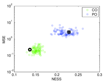
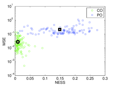
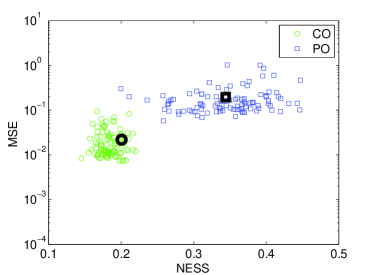
Figure 1: Performance of the pMCMC (left) and the NPMC (right) methods for the estimation of a unique rate parameter θ1subscript𝜃1\theta_{1}: MSE (in logarithmic scale) obtained from the final output versus the NESS for each simulation run in the CO and the PO scenario. The big circles and squares represent simulation runs with a final mean MSE close to the global average
Refer to caption
Refer to caption
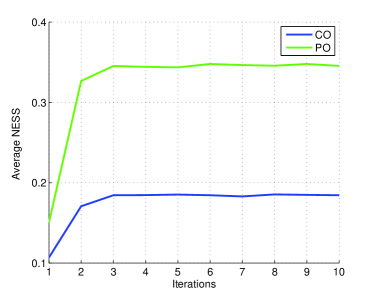
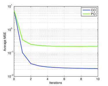
Figure 2: Evolution along the iterations of the NPMC algorithm of the average NESS (left) and MSE (right) in the CO and PO scenarios, estimating a single parameter θ1subscript𝜃1\theta_{1}.

5.4 Simulation results

We consider two simulation scenarios in which a different number of parameters is estimated.

5.4.1 Estimation of a single rate parameter θ1subscript𝜃1\theta_{1}

In this section we present numerical results regarding the approximation of the posterior distribution p(θ1,x|𝜽\1,y)𝑝subscript𝜃1conditionalxsubscript𝜽\absent1yp(\theta_{1},\textbf{x}|{\boldsymbol{\theta}}_{\backslash 1},\textbf{y}) of a single rate parameter θ1=logc1subscript𝜃1subscript𝑐1\theta_{1}=\log c_{1} and the populations x, when the rest of parameters 𝜽\1=[θ2,,θK]subscript𝜽\absent1superscriptsubscript𝜃2subscript𝜃𝐾top{\boldsymbol{\theta}}_{\backslash 1}=[\theta_{2},\ldots,\theta_{K}]^{\top}, are assumed to be known.

We compare the pMCMC and the NPMC methods in this simple scenario in order to illustrate the optimal performance of both schemes, in the CO and PO scenarios. This simulations show the degradation of the approximations when the amount of observations reduces.

We have performed P=100𝑃100P=100 independent simulation runs of the pMCMC and the NPMC schemes in the CO and the PO scenarios, with different (independent) population and observation vectors in each simulation. Both in the CO and the PO cases, the same true population trajectories x(p)superscriptx𝑝\textbf{x}^{(p)}, p=1,,P𝑝1𝑃p=1,\ldots,P, were used, but the observations in the CO scenario, yCO(p)superscriptsubscripty𝐶𝑂𝑝\textbf{y}_{CO}^{(p)}, and in the PO scenario, yPO(p)superscriptsubscripty𝑃𝑂𝑝\textbf{y}_{PO}^{(p)}, differ. The number of observation times has been set to N=100𝑁100N=100.

As a proposal pdf q(𝜽|𝜽)𝑞conditionalsuperscript𝜽𝜽q({\boldsymbol{\theta}}^{\star}|{\boldsymbol{\theta}}) in the pMCMC scheme we consider a Gaussian random walk update with variance γ2=1superscript𝛾21\gamma^{2}=1, which to the best results in the simulations. A total number of I=104𝐼superscript104I=10^{4} iterations has been run in each simulation. A final sample of size M=103𝑀superscript103M=10^{3} has been obtained from each Markov chain by discarding a burn-in period of 103superscript10310^{3} samples and thinning the output by a factor of 9.

In the NPMC scheme, the number of iterations has been set to L=10𝐿10L=10, the number of samples per iteration is M=103𝑀superscript103M=10^{3} and the clipping parameter is MT=100subscript𝑀𝑇100M_{T}=100. In this way, the computational effort of the two methods is approximately the same, as they both generate 104superscript10410^{4} samples in the space of 𝜽𝜽{\boldsymbol{\theta}}.

In Figure 1 the final MSE obtained by the pMCMC (left) and the NPMC (right) algorithms for each simulation run is depicted versus the final NESS, in the CO and the PO scenarios. Note that the NESS is computed differently for pMCMC and NPMC. It can be observed that both algorithms perform similarly in this case, with an equivalent computational cost. Both algorithms attain on average lower MSE values in the CO scenario, as expected. However, the NESS also takes lower values in the CO case, which indicates a worse mixing of the Markov chains in the pMCMC algorithm and also higher degeneracy in the NPMC algorithm.
Refer to caption
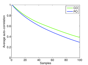
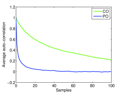
Figure 3: Average ACF based on the final sample of size M=103𝑀superscript103M=10^{3} of the pMCMC scheme in the CO and the PO scenarios, averaged over P=100𝑃100P=100 simulation runs

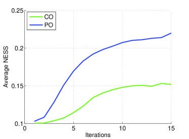
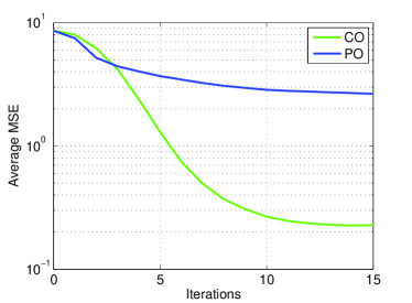
In Figure 2 the evolution of the MSE (right) and the NESS (left) along the iterations of the NPMC algorithm is represented, for the CO and the PO scenarios. It can be observed that both measures attain a steady value by the 5-th iteration, both in the CO and the PO case, which suggest that actually less iterations are sufficient for this problem. Again, we observe that in the CO scenario both the NESS and the MSE reach lower values.

Figure 3 plots the average ACF of the final pMCMC sample, after removing the burn-in period and thinning the Markov chain by a factor of 9. Particularly high correlations are present in the CO case, leading to a poor NESS. Related to the ACF, the average sample acceptance probability in the pMCMC scheme in the PO scenario is 0.091, while in the CO scenario it is only 0.0034. Which means that 910 samples are accepted out of I=104𝐼superscript104I=10^{4} in the CO case and only 34 in the CO case.

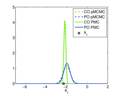
In Figure 4 the final pdf estimates p^(θ1|𝜽\1,y)^𝑝conditionalsubscript𝜃1subscript𝜽\absent1y\hat{p}(\theta_{1}|{\boldsymbol{\theta}}_{\backslash 1},\textbf{y}) of the average simulation runs represented as big circles and crosses in Figure 1 are represented in the CO and the PO scenario, for the pMCMC and the NPMC schemes. For the pMCMC method we have built a Gaussian approximation of the posterior density p(θ1|𝜽\1,y)𝑝conditionalsubscript𝜃1subscript𝜽\absent1yp(\theta_{1}|{\boldsymbol{\theta}}_{\backslash 1},\textbf{y}) based on the final MCMC sample {θ1(i)}i=1Msuperscriptsubscriptsuperscriptsubscript𝜃1𝑖𝑖1𝑀\{\theta_{1}^{(i)}\}_{i=1}^{M}. For the NPMC method, this approximation corresponds to the proposal pdf for the next iteration L+1𝐿1L+1, i.e., p^(θ1|𝜽\1,y)=qL+1(θ1)=𝒩(θ1;μL,1,σL,12)^𝑝conditionalsubscript𝜃1subscript𝜽\absent1ysubscript𝑞𝐿1subscript𝜃1𝒩subscript𝜃1subscript𝜇𝐿1superscriptsubscript𝜎𝐿12\hat{p}(\theta_{1}|{\boldsymbol{\theta}}_{\backslash 1},\textbf{y})=q_{L+1}(\theta_{1})=\mathcal{N}(\theta_{1};\mu_{L,1},\sigma_{L,1}^{2}), where the mean and variance terms μL,1subscript𝜇𝐿1\mu_{L,1} and σL,12superscriptsubscript𝜎𝐿12\sigma_{L,1}^{2} are computed as in Eq. (4). It can be observed in Figure 4 that very similar results are obtained by both algorithms in this scenario. The final MSE values obtained by the pMCMC and the NPMC methods, averaged over P=100𝑃100P=100 simulation runs, are shown in Table 3, together with the MSE corresponding to the prior distribution.
Refer to caption
Figure 4: Marginal posterior pdf estimates p^(θ1,|𝜽\1,y)\hat{p}(\theta_{1},|{\boldsymbol{\theta}}_{\backslash 1},\textbf{y}) of an average simulation run, for pMCMC and NPMC in the CO and PO scenarios. The true value θ1subscript𝜃1\theta_{1} is also shown
Table 3: Final mean and standard deviation (std) values of the MSE for θ1subscript𝜃1\theta_{1} in the CO and PO scenarios, for pMCMC and NPMC. The prior values are included for comparison
mean MSE std MSE
Prior 6.789 0
PO pMCMC 0.215 0.171
NPMC 0.195 0.170
CO pMCMC 0.027 0.026
NPMC 0.022 0.016
Refer to caption
Refer to caption
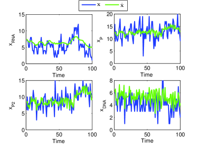
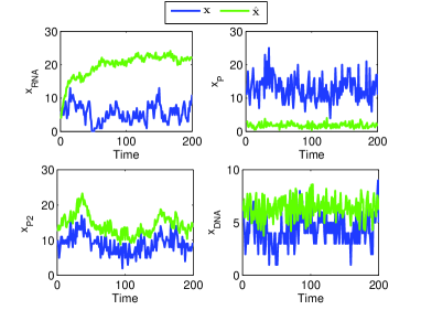
Figure 5: Posterior mean, x^=Ep^(x|y)[x]^xsubscript𝐸^𝑝conditionalxydelimited-[]x\hat{\textbf{x}}=E_{\hat{p}(\textbf{x}|\textbf{y})}[\textbf{x}], of the populations obtained in a single simulation run of pMCMC (left) and NPMC (right) in the PO scenario (only a linear combination of the proteins is observed, corrupted by noise)

Figure 5 depicts the posterior mean of the populations, x^=Ep^(x|y)[x]^xsubscript𝐸^𝑝conditionalxydelimited-[]x\hat{\textbf{x}}=E_{\hat{p}(\textbf{x}|\textbf{y})}[\textbf{x}], obtained with pMCMC (left) as x^=1Mi=1Mx(i)^x1𝑀superscriptsubscript𝑖1𝑀superscriptx𝑖\hat{\textbf{x}}=\frac{1}{M}\sum_{i=1}^{M}\textbf{x}^{(i)} and with NPMC (right) as x^=i=1Mw¯L(i)xL(i)^xsuperscriptsubscript𝑖1𝑀superscriptsubscript¯𝑤𝐿𝑖superscriptsubscriptx𝐿𝑖\hat{\textbf{x}}=\sum_{i=1}^{M}\bar{w}_{L}^{(i)}\textbf{x}_{L}^{(i)} in the PO scenario. The results correspond to the particular simulation runs (different for pMCMC and NPMC) identified with big squares in Figure 1 and whose posterior approximations, p^(θ1|𝜽\1,y)^𝑝conditionalsubscript𝜃1subscript𝜽\absent1y\hat{p}(\theta_{1}|{\boldsymbol{\theta}}_{\backslash 1},\textbf{y}), are shown in Figure 4. It can be observed that, in the PO scenario, the tendency of the population of all the species is reasonably identified, even though only a linear combination of the proteins is observed. In the CO scenario the populations of all species are accurately estimated and are not shown for conciseness. Note that the populations of all species are very low, which suggests that the diffusion approximation may perform poorly in this scenario.

The results presented in this section reveal a very similar performance of the two methods in this simple scenario. Also in terms of computational complexity pMCMC and NPMC perform very similarly. The execution time per 103superscript10310^{3} samples (one NPMC iteration and 103superscript10310^{3} pMCMC iterations) for the pMCMC scheme is 312 seconds, while for NPMC it is 325 seconds, both in the CO and in the PO cases, on a 3-GHz Intel Core 2 Duo CPU, with 2 GB of RAM. The stochastic forward simulation of the prokaryotic model with the Gillespie algorithm has been implemented in C, and the rest of the code in Matlab R2007b.

However, the pMCMC method provides a set of highly correlated samples, specially in the CO scenario, and requires the setting of the proposal variance γ2superscript𝛾2\gamma^{2} as well as the burn-in period length and the thinning parameter, which may not be straightforward and determines the performance of the algorithm. On the contrary, the NPMC scheme provides uncorrelated sets of samples at each iteration, and does not require the precise fitting of any parameters. Additionally, the computer simulations suggest that the convergence of the NPMC algorithm may be assessed observing the evolution of the NESS, which usually reaches a steady value simultaneously with the MSE.

5.4.2 Estimation of all the parameters θksubscript𝜃𝑘\theta_{k}, k=1,,K𝑘1𝐾k=1,\ldots,K

In this section we present simulation results to evaluate the performance of the pMCMC and the NPMC schemes in the approximation of the posterior distribution of the rate parameters and the populations of all species, p(𝜽,x|y)𝑝𝜽conditionalxyp({\boldsymbol{\theta}},\textbf{x}|\textbf{y}), assuming that all the rate parameters are unknown, again in the CO and the PO scenarios.

In this case, N=200𝑁200N=200 observation times are assumed for all the simulations. Again, P=100𝑃100P=100 independent simulation runs of each algorithm have been performed. The NPMC scheme has been run for L=15𝐿15L=15 iterations, with M=103𝑀superscript103M=10^{3} samples per iteration and clipping parameter MT=100subscript𝑀𝑇100M_{T}=100. The pMCMC scheme has been run with I=15×103𝐼15superscript103I=15\times 10^{3} iterations in each simulation run, a burn-in period of 103superscript10310^{3} iterations and thinning the output by a factor of 141414. With this setup the computational effort is approximately the same in the two schemes.
Refer to caption
Refer to caption
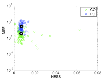
Figure 6: Performance of the pMCMC (left) and the NPMC (right) methods for the estimation of the whole set of rate parameters 𝜽𝜽{\boldsymbol{\theta}}: MSE (in logarithmic scale) versus the final NESS, for each simulation run in the CO and the PO scenario. The big circles and squares represent simulation runs with a final mean MSE close to the global average
Refer to caption
Refer to caption
Figure 7: Evolution along the NPMC iterations of the average NESS (left) and MSE (right) in the CO and the PO scenario.
Refer to caption
Refer to caption
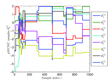
Figure 8: Left: Auto-correlations based on the final sample of size 103superscript10310^{3} of the pMCMC scheme in the CO and the PO scenarios, averaged over P=100𝑃100P=100 simulation runs. Right: Markov chain provided by the pMCMC method in the PO scenario, corresponding to the average simulation run depicted with a big square in Figure 8 (left).

In Figure 8 the MSE (in logarithmic scale), averaged over the parameters θksubscript𝜃𝑘\theta_{k}, attained by the pMCMC (left) and the NPMC (right) algorithms is represented versus the NESS, in the CO and PO scenarios. Simulation runs which attained a final MSE close to the global average value are indicated with big circles (CO) and squares (PO) on both plots. It can be observed that the pMCMC method performs similarly in both scenarios, in terms of MSE and NESS, yielding poor results in both cases. On the contrary, the NPMC method provides significantly better MSE𝑀𝑆𝐸MSE results in the CO scenario, where a larger amount of information is available. The NPMC method does not present degradation due to the high degeneracy occurring in the CO scenario.
Refer to caption
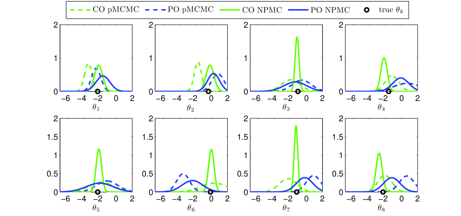
Figure 9: Marginal posterior pdf approximations of each parameter p^(θk|y)^𝑝conditionalsubscript𝜃𝑘y\hat{p}(\theta_{k}|\textbf{y}), k=1,,K𝑘1𝐾k=1,\ldots,K, attained in an average simulation run by the pMCMC and the NPMC, in the CO and in the PO case.
Figure 10: Final MSE for the parameters θksubscript𝜃𝑘\theta_{k}, k=1,,K𝑘1𝐾k=1,\ldots,K in the CO and PO experiments, averaged over the simulation runs. The last two columns corresponds to the mean and standard deviation (std) values of the global MSE (averaged over the parameters). The prior values are included for comparison
θ1subscript𝜃1\theta_{1} θ2subscript𝜃2\theta_{2} θ3subscript𝜃3\theta_{3} θ4subscript𝜃4\theta_{4} θ5subscript𝜃5\theta_{5} θ6subscript𝜃6\theta_{6} θ7subscript𝜃7\theta_{7} θ8subscript𝜃8\theta_{8} mean MSE std MSE
Prior 6.789 11.344 8.853 7.543 6.789 12.484 8.430 6.789 8.628 0
PO pMCMC 3.412 3.319 5.543 3.200 7.059 8.929 6.799 4.371 5.329 2.926
NPMC 1.246 1.011 2.214 1.490 4.073 7.015 2.311 1.856 2.652 1.020
CO pMCMC 2.899 2.958 1.676 1.572 1.604 1.547 1.573 1.468 1.912 1.476
NPMC 0.305 0.302 0.162 0.167 0.280 0.280 0.156 0.168 0.228 0.091
Refer to caption
Refer to caption
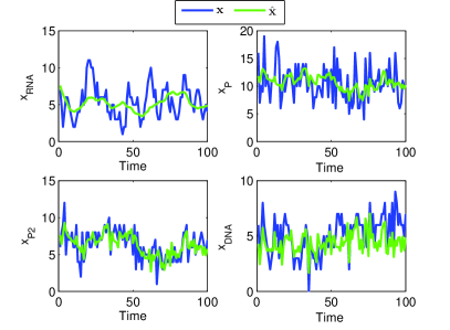
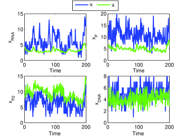
Figure 11: Posterior mean x^=Ep(x|y)[x]^xsubscript𝐸𝑝conditionalxydelimited-[]x\hat{\textbf{x}}=E_{p(\textbf{x}|\textbf{y})}[\textbf{x}] of the populations of all species obtained in the average simulation run of the pMCMC (left) and the NPMC (right) schemes, in the PO scenario.

Figure 8 depicts the evolution along the iterations of the NESS (left) and the MSE (right) averaged over P=100𝑃100P=100 independent simulation runs for the NPMC algorithm. Both indices converge to a steady value in a low number of iterations also in this complex scenario. As expected, a significantly higher final MSE is attained in the extremely data poor PO scenario.

In Figure 8 (left) the average ACF attained by the pMCMC in the CO and the PO cases is represented. Even after thinning the output, the sample correlation is extremely high in both scenarios, which leads to a very low NESS. The acceptance rate is also very low and very long chains are required to obtain reasonable results. In the PO scenario 43.69 samples are accepted on average in a simulation run of I=15×103𝐼15superscript103I=15\times 10^{3} samples (acceptance rate 0.0029). In the CO case, only 23.07 samples are accepted on average (rate 0.0015).

Figure 8 (right) depicts the final Markov chain provided by the pMCMC method (after removing the burn-in period and thinning the output) in the average simulation run represented with a big square in Figure 8 (left). It can be observed that the mixing of the chain is very poor, with a total number of accepted samples of 46 (close to the average). Many other simulations, both in the PO and the CO scenarios, provide even lower number of accepted samples, and thus, very inconsistent results.

Figure 11 depicts the final Gaussian approximations of the marginal posteriors p(θk|y)𝑝conditionalsubscript𝜃𝑘yp(\theta_{k}|\textbf{y}), k=1,,8𝑘18k=1,\ldots,8, obtained by the pMCMC and the NPMC methods, in the CO and PO scenarios, for the average simulation runs represented as big circles and squares in Figure 8. We can observe that the NPMC method provides a significantly better approximation of the log-rate parameters in the CO scenario, where a larger amount of data is available, which is also clear from Figure 8 (right). However, the pMCMC on average performs similarly in both scenarios, due to the low efficiency of the pMCMC sampling scheme when the dimension of the problem (either K𝐾K or N𝑁N) increases.

In Table 11 the MSE of each parameter θksubscript𝜃𝑘\theta_{k} averaged over P=100𝑃100P=100 independent simulation runs is shown, as obtained with the pMCMC and the NPMC schemes, for the CO and the PO experiments. In the CO case, NPMC provides homogeneous results for all parameters. On the contrary, in the PO case, some of the parameters (specially θ5subscript𝜃5\theta_{5} and θ6subscript𝜃6\theta_{6}) are significantly poorly estimated, presenting a final MSE close to the initial value (which corresponds to the prior knowledge). The pMCMC scheme presents significantly higher MSE values than NPMC in both observation scenarios and for all parameters θksubscript𝜃𝑘\theta_{k}.

Figure 11 depicts the population posterior mean x^=Ep(x|y)[x]^xsubscript𝐸𝑝conditionalxydelimited-[]x\hat{\textbf{x}}=E_{p(\textbf{x}|\textbf{y})}[\textbf{x}] corresponding to the average simulation runs of the pMCMC and the NPMC methods in the PO scenario, represented as big squares in Figure 8. Again, the NPMC method provides more accurate estimates of the unobserved populations than the pMCMC method, specially for xRNAsubscript𝑥𝑅𝑁𝐴x_{RNA}. In the CO scenario both methods provide good approximations of the populations of all species.

6 Asymptotic convergence of NIS with approximate weights

6.1 Scope of the analysis

An analysis of the asymptotic effect of the transformation of the weights on the IS-based approximation of integrals w.r.t. a target probability distribution has already been addressed in (Koblents and Míguez, 2013b). In particular, the results in (Koblents and Míguez, 2013b) show that, as long as MTM0subscript𝑀𝑇𝑀0\frac{M_{T}}{M}\rightarrow 0, the distortion introduced by the clipping of the weights vanishes asymptotically and the approximation of integrals of bounded functions using IWs and using TIWs both converge to the same value almost surely (a.s.). However,

  • the argument in (Koblents and Míguez, 2013b) is based on classical concentration-of-measure inequalities and, therefore, rates are only found for convergence in probability, and

  • more importantly, the analysis relies on the ability to compute the non-normalized IWs exactly.

It is apparent from the algorithm description in Section 4 that, in the case of the SKM models of interest in this paper, the IWs can only be approximated (via particle filtering) and, therefore, the assumptions on which the theoretical results of (Koblents and Míguez, 2013b) rely are not satisfied. In this section, we improve on the analysis in (Koblents and Míguez, 2013b) by looking explicitly into the convergence of the approximations of integrals computed using approximate weights (both IWs and TIWs). We provide convergence rates for the Lpsubscript𝐿𝑝L_{p} norms of the approximation errors and show that the approximate weights computed by a standard particle filter are “good enough” to ensure that these results hold.

6.2 Notation and basic assumptions

Let π(𝜽)𝜋𝜽\pi({\boldsymbol{\theta}}) be the pdf associated to the target probability distribution, let q(𝜽)𝑞𝜽q({\boldsymbol{\theta}}) be the importance function used to propose samples in an IS scheme (not necessarily normalized) and let h(𝜽)π(𝜽)proportional-to𝜽𝜋𝜽h({\boldsymbol{\theta}})\propto\pi({\boldsymbol{\theta}}) be a function proportional to π𝜋\pi, with the proportionality constant independent of 𝜽𝜽{\boldsymbol{\theta}}. The samples drawn from the distribution associated to q𝑞q are denoted 𝜽(i)superscript𝜽𝑖{\boldsymbol{\theta}}^{(i)}, i=1,,M𝑖1𝑀i=1,...,M, and their associated non-normalized IWs are w(i)=h(𝜽(i))/q(𝜽(i))superscript𝑤𝑖superscript𝜽𝑖𝑞superscript𝜽𝑖w^{(i)*}=h({\boldsymbol{\theta}}^{(i)})/q({\boldsymbol{\theta}}^{(i)}), i=1,,M𝑖1𝑀i=1,...,M.

Let us define the weight function g(𝜽)=h(𝜽)/q(𝜽)𝑔𝜽𝜽𝑞𝜽g({\boldsymbol{\theta}})=h({\boldsymbol{\theta}})/q({\boldsymbol{\theta}}) and, in particular, g(𝜽(i))=w(i)𝑔superscript𝜽𝑖superscript𝑤𝑖g({{\boldsymbol{\theta}}}^{(i)})=w^{(i)*}. The support of g𝑔g is the same as the support of q𝑞q, denoted 𝖲K𝖲superscript𝐾{\sf S}\subseteq\mathbb{R}^{K}. If we assume that both q(𝜽)>0𝑞𝜽0q({\boldsymbol{\theta}})>0 and π(𝜽)>0𝜋𝜽0\pi({\boldsymbol{\theta}})>0 for any 𝜽𝖲𝜽𝖲{\boldsymbol{\theta}}\in{\sf S}, then g(𝜽)>0𝑔𝜽0g({\boldsymbol{\theta}})>0 for every 𝜽𝖲𝜽𝖲{\boldsymbol{\theta}}\in{\sf S} as well. Also, trivially, πgqproportional-to𝜋𝑔𝑞\pi\propto gq, with the proportionality constant independent of 𝜽𝜽{\boldsymbol{\theta}}. These assumptions are standard for classical IS.

Assume that the standard IWs can be computed exactly. In that case, the approximation πMsuperscript𝜋𝑀\pi^{M} of the target probability measure can be written as

πM(d𝜽)=i=1Mw(i)δ𝜽(i)(d𝜽),superscript𝜋𝑀𝑑𝜽superscriptsubscript𝑖1𝑀superscript𝑤𝑖subscript𝛿superscript𝜽𝑖𝑑𝜽\pi^{M}(d{\boldsymbol{\theta}})=\sum_{i=1}^{M}w^{(i)}\delta_{{{\boldsymbol{\theta}}}^{(i)}}(d{\boldsymbol{\theta}}),

where w(i)=g(𝜽(i))j=1Mg(𝜽(j))superscript𝑤𝑖𝑔superscript𝜽𝑖superscriptsubscript𝑗1𝑀𝑔superscript𝜽𝑗w^{(i)}=\frac{g({{\boldsymbol{\theta}}}^{(i)})}{\sum_{j=1}^{M}g({{\boldsymbol{\theta}}}^{(j)})}, i=1,,M𝑖1𝑀i=1,...,M.

Assume next that the weight function cannot be evaluated exactly but, instead, a sequence of approximations gJ(𝜽)superscript𝑔𝐽𝜽g^{J}({\boldsymbol{\theta}}), J𝐽J\in\mathbb{N}, exists for any point 𝜽𝖲𝜽𝖲{\boldsymbol{\theta}}\in{\sf S}. We denote the random measure constructed from the approximate IWs as

πM,J(d𝜽)=i=1Mw(i),Jδ𝜽(i)(d𝜽),superscript𝜋𝑀𝐽𝑑𝜽superscriptsubscript𝑖1𝑀superscript𝑤𝑖𝐽subscript𝛿superscript𝜽𝑖𝑑𝜽\pi^{M,J}(d{\boldsymbol{\theta}})=\sum_{i=1}^{M}w^{(i),J}\delta_{{{\boldsymbol{\theta}}}^{(i)}}(d{\boldsymbol{\theta}}),

where w(i),J=gJ(𝜽(i))j=1MgJ(𝜽(j))superscript𝑤𝑖𝐽superscript𝑔𝐽superscript𝜽𝑖superscriptsubscript𝑗1𝑀superscript𝑔𝐽superscript𝜽𝑗w^{(i),J}=\frac{g^{J}({{\boldsymbol{\theta}}}^{(i)})}{\sum_{j=1}^{M}g^{J}({{\boldsymbol{\theta}}}^{(j)})}, i=1,,M𝑖1𝑀i=1,...,M. Let us denote by φMsuperscript𝜑𝑀\varphi^{M} the nonlinear transformation function used to compute non-normalized TIWs, i.e., w¯(i)=φM(w(i))superscript¯𝑤𝑖superscript𝜑𝑀superscript𝑤𝑖\bar{w}^{(i)*}=\varphi^{M}(w^{(i)*}), i=1,,M𝑖1𝑀i=1,\ldots,M, where w(i)superscript𝑤𝑖w^{(i)*} is the standard unnormalized IW associated to the sample 𝜽(i)superscript𝜽𝑖{\boldsymbol{\theta}}^{(i)}. Then the weighted approximation of π(𝜽)d𝜽𝜋𝜽𝑑𝜽\pi({\boldsymbol{\theta}})d{\boldsymbol{\theta}} constructed according to the NIS scheme is

π¯M,J(d𝜽)=i=1Mw¯(i),Jδ𝜽(i)(d𝜽),superscript¯𝜋𝑀𝐽𝑑𝜽superscriptsubscript𝑖1𝑀superscript¯𝑤𝑖𝐽subscript𝛿superscript𝜽𝑖𝑑𝜽\bar{\pi}^{M,J}(d{\boldsymbol{\theta}})=\sum_{i=1}^{M}\bar{w}^{(i),J}\delta_{{{\boldsymbol{\theta}}}^{(i)}}(d{\boldsymbol{\theta}}),

where w¯(i),J=φM(gJ(𝜽(i)))j=1MφM(gJ(𝜽(j)))superscript¯𝑤𝑖𝐽superscript𝜑𝑀superscript𝑔𝐽superscript𝜽𝑖superscriptsubscript𝑗1𝑀superscript𝜑𝑀superscript𝑔𝐽superscript𝜽𝑗\bar{w}^{(i),J}=\frac{\varphi^{M}(g^{J}({{\boldsymbol{\theta}}}^{(i)}))}{\sum_{j=1}^{M}\varphi^{M}(g^{J}({{\boldsymbol{\theta}}}^{(j)}))}, i=1,,M𝑖1𝑀i=1,...,M.

We make the following assumptions on the transformation function φMsuperscript𝜑𝑀\varphi^{M}, the weight function g𝑔g and its approximations {gJ:J1}conditional-setsuperscript𝑔𝐽𝐽1\{g^{J}:J\geq 1\}.

  • A1

    The nonlinear transformation φMsuperscript𝜑𝑀\varphi^{M} of the weights is of a clipping class. In particular, given an index permutation i1,,iMsubscript𝑖1subscript𝑖𝑀i_{1},\ldots,i_{M} such that w(i1)w(iM)superscript𝑤subscript𝑖1superscript𝑤subscript𝑖𝑀w^{(i_{1})*}\geq\ldots\geq w^{(i_{M})*}, and a choice of the clipping parameter MT<Msubscript𝑀𝑇𝑀M_{T}<M, the transformation φMsuperscript𝜑𝑀\varphi^{M} can be expressed as222Note that φMsuperscript𝜑𝑀\varphi^{M} is a function of both the complete weight set {w(j)}j=1Msuperscriptsubscriptsuperscript𝑤𝑗𝑗1𝑀\{w^{(j)*}\}_{j=1}^{M} and the index of the weight to be transformed, i.e., φM:{w(j),j=1,,M}×{1,,M}[1,+)\varphi^{M}:\{w^{(j)*},j=1,\ldots,M\}\times\{1,\ldots,M\}\rightarrow[1,+\infty).

    φM(w(ik))={w(iMT),for k=1,,MT,andw(ik),for k=MT+1,,M..superscript𝜑𝑀superscript𝑤subscript𝑖𝑘casessuperscript𝑤subscript𝑖subscript𝑀𝑇for 𝑘1subscript𝑀𝑇andsuperscript𝑤subscript𝑖𝑘for 𝑘subscript𝑀𝑇1𝑀\varphi^{M}(w^{(i_{k})*})\!=\!\left\{\begin{array}[]{ll}w^{(i_{M_{T}})*},&\mbox{for }k=1,\ldots,M_{T},\;\mbox{and}\\ w^{(i_{k})*},&\mbox{for }k=M_{T}+1,\ldots,M.\end{array}\right..
  • A2

    The weight function g𝑔g has a finite upper bound and a positive lower bound. Specifically, there exists a real number 0<a<0𝑎0<a<\infty such that a1g(𝜽)asuperscript𝑎1𝑔𝜽𝑎a^{-1}\leq g({\boldsymbol{\theta}})\leq a for every 𝜽𝖲𝜽𝖲{\boldsymbol{\theta}}\in{\sf S}.

  • A3

    The same bounds of the weight function g𝑔g hold for its approximations gJsuperscript𝑔𝐽g^{J}, J1𝐽1J\geq 1. To be specific, the inequalities a1gJ(𝜽)asuperscript𝑎1superscript𝑔𝐽𝜽𝑎a^{-1}\leq g^{J}({\boldsymbol{\theta}})\leq a hold for every 𝜽𝖲𝜽𝖲{\boldsymbol{\theta}}\in{\sf S}, any J1𝐽1J\geq 1 and the same real number 0<a<0𝑎0<a<\infty as in A2.

  • A4

    The approximation gJsuperscript𝑔𝐽g^{J} of the weight function is possibly random and satisfies the inequality

    sup𝜽𝖲|g(𝜽)gJ(𝜽)|Wg,ϵJ12ϵsubscriptsupremum𝜽𝖲𝑔𝜽superscript𝑔𝐽𝜽subscript𝑊𝑔italic-ϵsuperscript𝐽12italic-ϵ\sup_{{\boldsymbol{\theta}}\in{\sf S}}|g({\boldsymbol{\theta}})-g^{J}({\boldsymbol{\theta}})|\leq\frac{W_{g,\epsilon}}{J^{\frac{1}{2}-\epsilon}}

    where Wg,ϵsubscript𝑊𝑔italic-ϵW_{g,\epsilon} is a positive a.s. finite random variable and 0<ϵ<120italic-ϵ120<\epsilon<\frac{1}{2} is an arbitrarily small constant, both independent of J𝐽J.

Note that if the support set 𝖲𝖲{\sf S} is compact then assumption A2 holds whenever q>0𝑞0q>0 and h>00h>0 in 𝖲𝖲{\sf S}. Otherwise, the proposal q𝑞q has to be chosen so that it has heavier tails than π𝜋\pi.

In the sequel we look into the approximation of integrals of the form (f,π)=I𝖲(𝜽)f(𝜽)π(𝜽)𝑑𝜽𝑓𝜋subscript𝐼𝖲𝜽𝑓𝜽𝜋𝜽differential-d𝜽(f,\pi)=\int I_{{\sf S}}({\boldsymbol{\theta}})f({\boldsymbol{\theta}})\pi({\boldsymbol{\theta}})d{\boldsymbol{\theta}}, where I𝖲(𝜽)subscript𝐼𝖲𝜽I_{\sf S}({\boldsymbol{\theta}}) is an indicator function333Namely, I𝖲(𝜽)=1subscript𝐼𝖲𝜽1I_{\sf S}({\boldsymbol{\theta}})=1 if 𝜽𝖲𝜽𝖲{\boldsymbol{\theta}}\in{\sf S} and I𝖲(𝜽)=0subscript𝐼𝖲𝜽0I_{\sf S}({\boldsymbol{\theta}})=0 otherwise. and f𝑓f is a bounded real function in the parameter space 𝖲𝖲{\sf S}. We use f=sup𝜽𝖲|f(𝜽)|<subscriptnorm𝑓subscriptsupremum𝜽𝖲𝑓𝜽\|f\|_{\infty}=\sup_{{\boldsymbol{\theta}}\in{\sf S}}|f({\boldsymbol{\theta}})|<\infty to denote the supremum norm of a bounded function. The set of bounded functions on 𝖲𝖲{\sf S} is B(𝖲)={f:𝖲:f<}𝐵𝖲conditional-set𝑓:𝖲subscriptnorm𝑓B({\sf S})=\{f:{\sf S}\rightarrow\mathbb{R}:\|f\|_{\infty}<\infty\}. The approximations of interest are

(f,πM,J)𝑓superscript𝜋𝑀𝐽\displaystyle(f,\pi^{M,J}) =\displaystyle= i=1Mf(𝜽(i))w(i),J,andsuperscriptsubscript𝑖1𝑀𝑓superscript𝜽𝑖superscript𝑤𝑖𝐽and\displaystyle\sum_{i=1}^{M}f({\boldsymbol{\theta}}^{(i)})w^{(i),J},\quad\mbox{and}
(f,π¯M,J)𝑓superscript¯𝜋𝑀𝐽\displaystyle(f,\bar{\pi}^{M,J}) =\displaystyle= i=1Mf(𝜽(i))w¯(i),J.superscriptsubscript𝑖1𝑀𝑓superscript𝜽𝑖superscript¯𝑤𝑖𝐽\displaystyle\sum_{i=1}^{M}f({\boldsymbol{\theta}}^{(i)})\bar{w}^{(i),J}.

6.3 Convergence rates

The following basic Lemma establishes that both (f,π¯M,J)𝑓superscript¯𝜋𝑀𝐽(f,\bar{\pi}^{M,J}) and (f,π¯M,J)𝑓superscript¯𝜋𝑀𝐽(f,\bar{\pi}^{M,J}) converge toward (f,π)𝑓𝜋(f,\pi) a.s. and provides explicit rates for the absolute approximation errors.

Lemma 1

Assume that A1, A2, A3 and A4 hold,

J=J(M)MandMTM.formulae-sequence𝐽𝐽𝑀𝑀andsubscript𝑀𝑇𝑀J=J(M)\geq M\quad\mbox{and}\quad M_{T}\leq\sqrt{M}.

Then, there exist positive and a.s. finite random variables Wf,g,ϵsubscript𝑊𝑓𝑔italic-ϵW_{f,g,\epsilon} and W¯f,g,ϵsubscript¯𝑊𝑓𝑔italic-ϵ\bar{W}_{f,g,\epsilon}, independent of M𝑀M and J𝐽J, such that

|(f,πM,J)(f,π)|Wf,g,ϵM12ϵ𝑓superscript𝜋𝑀𝐽𝑓𝜋subscript𝑊𝑓𝑔italic-ϵsuperscript𝑀12italic-ϵ|(f,\pi^{M,J})-(f,\pi)|\leq\frac{W_{f,g,\epsilon}}{M^{\frac{1}{2}-\epsilon}} (6)

and

|(f,π¯M,J)(f,π)|W¯f,g,ϵM12ϵ𝑓superscript¯𝜋𝑀𝐽𝑓𝜋subscript¯𝑊𝑓𝑔italic-ϵsuperscript𝑀12italic-ϵ|(f,\bar{\pi}^{M,J})-(f,\pi)|\leq\frac{\bar{W}_{f,g,\epsilon}}{M^{\frac{1}{2}-\epsilon}} (7)

for every fB(𝖲)𝑓𝐵𝖲f\in B({\sf S}), where 0<ϵ<120italic-ϵ120<\epsilon<\frac{1}{2} is an arbitrarily small constant independent of M𝑀M and J𝐽J. In particular

limM(f,πM,J)=limM(f,π¯M,J)=(f,π) a.s.subscript𝑀𝑓superscript𝜋𝑀𝐽subscript𝑀𝑓superscript¯𝜋𝑀𝐽𝑓𝜋 a.s.\lim_{M\rightarrow\infty}(f,\pi^{M,J})=\lim_{M\rightarrow\infty}(f,\bar{\pi}^{M,J})=(f,\pi)\mbox{ a.s.} (8)

A proof is provided in Appendix B. Lemma 1 shows that we attain the usual Monte Carlo rate of convergence (M12+ϵsuperscript𝑀12italic-ϵM^{-\frac{1}{2}+\epsilon}) despite the approximation of the IWs and its subsequent clipping to compute TIWs. Note, however, that the random variables Wf,g,ϵsubscript𝑊𝑓𝑔italic-ϵW_{f,g,\epsilon} and W¯f,g,ϵsubscript¯𝑊𝑓𝑔italic-ϵ\bar{W}_{f,g,\epsilon} are not equal and, in general, Wf,g,ϵW¯f,g,ϵsubscript𝑊𝑓𝑔italic-ϵsubscript¯𝑊𝑓𝑔italic-ϵW_{f,g,\epsilon}\leq\bar{W}_{f,g,\epsilon}.

6.4 Approximate weights via particle filtering

In this section we introduce a more precise notation for the state-space model (compared to the argument-wise used in the previous sections), in order to perform the analysis with approximate weights. Assume we have a discrete-time state space Markov model with state process {Xn}n0subscriptsubscriptX𝑛𝑛0\{\textbf{X}_{n}\}_{n\geq 0} taking values on 𝒳dx𝒳superscriptsubscript𝑑x{\mathcal{X}}\subseteq\mathbb{R}^{d_{\textbf{x}}} and an observation process {Yn}n0subscriptsubscriptY𝑛𝑛0\{\textbf{Y}_{n}\}_{n\geq 0} taking values on 𝒴dy𝒴superscriptsubscript𝑑y{\mathcal{Y}}\subseteq\mathbb{R}^{d_{\textbf{y}}}. The prior distribution (probability measure) of the state is now denoted τ0(dx)subscript𝜏0𝑑x\tau_{0}(d\textbf{x}) and the transition (Markov) kernel depends on a vector-valued random parameter 𝚯𝚯\boldsymbol{\Theta} that takes values on a compact set 𝖲d𝜽𝖲superscriptsubscript𝑑𝜽{\sf S}\subset\mathbb{R}^{d_{{\boldsymbol{\theta}}}} and has prior distribution μ0(d𝜽)subscript𝜇0𝑑𝜽\mu_{0}(d{\boldsymbol{\theta}}) independent of X0subscriptX0\textbf{X}_{0}. In particular, the Markov kernel is now denoted τn,𝜽(dxn|xn1)subscript𝜏𝑛𝜽conditional𝑑subscriptx𝑛subscriptx𝑛1\tau_{n,{\boldsymbol{\theta}}}(d\textbf{x}_{n}|\textbf{x}_{n-1}) and the conditional density of the observations is un(yn|xn)>0subscript𝑢𝑛conditionalsubscripty𝑛subscriptx𝑛0u_{n}(\textbf{y}_{n}|\textbf{x}_{n})>0. The latter also yields the likelihood of the signal xnsubscriptx𝑛\textbf{x}_{n}, hence we often write, for conciseness, unyn(xn)un(yn|xn)superscriptsubscript𝑢𝑛subscripty𝑛subscriptx𝑛subscript𝑢𝑛conditionalsubscripty𝑛subscriptx𝑛u_{n}^{\textbf{y}_{n}}(\textbf{x}_{n})\triangleq u_{n}(\textbf{y}_{n}|\textbf{x}_{n}).

At time n𝑛n, the one-step-ahead predictive distribution of the state XnsubscriptX𝑛\textbf{X}_{n} given fixed observations Y1:n1=y1:n1subscriptY:1𝑛1subscripty:1𝑛1\textbf{Y}_{1:n-1}=\textbf{y}_{1:n-1} and a parameter value 𝚯=𝜽𝚯𝜽\boldsymbol{\Theta}={\boldsymbol{\theta}} is denoted ξn,𝜽subscript𝜉𝑛𝜽\xi_{n,{\boldsymbol{\theta}}}, specifically, for any Borel subset A𝒳𝐴𝒳A\subset{\mathcal{X}},

ξn,𝜽(A)=n(XnA|Y1:n1=y1:n1,𝚯=𝜽).\xi_{n,{\boldsymbol{\theta}}}(A)=\mathbb{P}_{n}\left(\textbf{X}_{n}\in A|\textbf{Y}_{1:n-1}=\textbf{y}_{1:n-1},\boldsymbol{\Theta}={\boldsymbol{\theta}}\right).

The filter measure at time n𝑛n given observations Y1:n=y1:nsubscriptY:1𝑛subscripty:1𝑛\textbf{Y}_{1:n}=\textbf{y}_{1:n} and parameter 𝚯=𝜽𝚯𝜽\boldsymbol{\Theta}={\boldsymbol{\theta}} is denoted ϕn,𝜽subscriptitalic-ϕ𝑛𝜽\phi_{n,{\boldsymbol{\theta}}}, namely,

ϕn,𝜽(A)=n(XnA|Y1:n=y1:n,𝚯=𝜽).\phi_{n,{\boldsymbol{\theta}}}(A)=\mathbb{P}_{n}\left(\textbf{X}_{n}\in A|\textbf{Y}_{1:n}=\textbf{y}_{1:n},\boldsymbol{\Theta}={\boldsymbol{\theta}}\right).

The predictive measure ξn,𝜽subscript𝜉𝑛𝜽\xi_{n,{\boldsymbol{\theta}}} can be expressed in terms of τn,𝜽subscript𝜏𝑛𝜽\tau_{n,{\boldsymbol{\theta}}} and ϕn1,𝜽subscriptitalic-ϕ𝑛1𝜽\phi_{n-1,{\boldsymbol{\theta}}}. Specifically, we write ξn,𝜽=τn,𝜽ϕn1,𝜽subscript𝜉𝑛𝜽subscript𝜏𝑛𝜽subscriptitalic-ϕ𝑛1𝜽\xi_{n,{\boldsymbol{\theta}}}=\tau_{n,{\boldsymbol{\theta}}}\phi_{n-1,{\boldsymbol{\theta}}}, meaning that, for any integrable function f:𝒳:𝑓𝒳f:{\mathcal{X}}\rightarrow\mathbb{R},

(f,ξn,𝜽)𝑓subscript𝜉𝑛𝜽\displaystyle(f,\xi_{n,{\boldsymbol{\theta}}}) =\displaystyle= f(x)τn,𝜽(dx|x)ϕn1,𝜽(dx)𝑓xsubscript𝜏𝑛𝜽conditional𝑑xsuperscriptxsubscriptitalic-ϕ𝑛1𝜽𝑑superscriptx\displaystyle\int\int f(\textbf{x})\tau_{n,{\boldsymbol{\theta}}}(d\textbf{x}|\textbf{x}^{\prime})\phi_{n-1,{\boldsymbol{\theta}}}(d\textbf{x}^{\prime})
=\displaystyle= (f,τn,𝜽ϕn1,𝜽).𝑓subscript𝜏𝑛𝜽subscriptitalic-ϕ𝑛1𝜽\displaystyle(f,\tau_{n,{\boldsymbol{\theta}}}\phi_{n-1,{\boldsymbol{\theta}}}).

We also note that

(f,ξn,𝜽)=(f¯n,ϕn1,𝜽),𝑓subscript𝜉𝑛𝜽subscript¯𝑓𝑛subscriptitalic-ϕ𝑛1𝜽(f,\xi_{n,{\boldsymbol{\theta}}})=(\bar{f}_{n},\phi_{n-1,{\boldsymbol{\theta}}}),

where f¯n(x)=f(x)τn,𝜽(dx|x)subscript¯𝑓𝑛superscriptx𝑓xsubscript𝜏𝑛𝜽conditional𝑑xsuperscriptx\bar{f}_{n}(\textbf{x}^{\prime})=\int f(\textbf{x})\tau_{n,{\boldsymbol{\theta}}}(d\textbf{x}|\textbf{x}^{\prime}). The filter measures ϕn,𝜽subscriptitalic-ϕ𝑛𝜽\phi_{n,{\boldsymbol{\theta}}} and ϕn1,𝜽subscriptitalic-ϕ𝑛1𝜽\phi_{n-1,{\boldsymbol{\theta}}} are related by the projective product

ϕn,𝜽=unynτn,𝜽ϕn1,𝜽=unynξn,𝜽,subscriptitalic-ϕ𝑛𝜽superscriptsubscript𝑢𝑛subscripty𝑛subscript𝜏𝑛𝜽subscriptitalic-ϕ𝑛1𝜽superscriptsubscript𝑢𝑛subscripty𝑛subscript𝜉𝑛𝜽\phi_{n,{\boldsymbol{\theta}}}=u_{n}^{\textbf{y}_{n}}\star\tau_{n,{\boldsymbol{\theta}}}\phi_{n-1,{\boldsymbol{\theta}}}=u_{n}^{\textbf{y}_{n}}\star\xi_{n,{\boldsymbol{\theta}}},

defined as (Bain and Crisan, 2008)

(f,unynξn,𝜽)(funyn,ξn,𝜽)(unyn,ξn,𝜽).𝑓superscriptsubscript𝑢𝑛subscripty𝑛subscript𝜉𝑛𝜽𝑓superscriptsubscript𝑢𝑛subscripty𝑛subscript𝜉𝑛𝜽superscriptsubscript𝑢𝑛subscripty𝑛subscript𝜉𝑛𝜽(f,u_{n}^{\textbf{y}_{n}}\star\xi_{n,{\boldsymbol{\theta}}})\triangleq\frac{(fu_{n}^{\textbf{y}_{n}},\xi_{n,{\boldsymbol{\theta}}})}{(u_{n}^{\textbf{y}_{n}},\xi_{n,{\boldsymbol{\theta}}})}.

Let

ξn,𝜽J(dx)=1Jj=1Jδxn(j)(dx) and superscriptsubscript𝜉𝑛𝜽𝐽𝑑x1𝐽superscriptsubscript𝑗1𝐽subscript𝛿superscriptsubscriptx𝑛𝑗𝑑x and \xi_{n,{\boldsymbol{\theta}}}^{J}(d\textbf{x})=\frac{1}{J}\sum_{j=1}^{J}\delta_{\textbf{x}_{n}^{(j)}}(d\textbf{x})\mbox{ and }
ϕn,𝜽J(dx)=1Jj=1Jδx~n(j)(dx)superscriptsubscriptitalic-ϕ𝑛𝜽𝐽𝑑x1𝐽superscriptsubscript𝑗1𝐽subscript𝛿superscriptsubscript~x𝑛𝑗𝑑x\phi_{n,{\boldsymbol{\theta}}}^{J}(d\textbf{x})=\frac{1}{J}\sum_{j=1}^{J}\delta_{\tilde{\textbf{x}}_{n}^{(j)}}(d\textbf{x})

be the approximations of ξn,𝜽subscript𝜉𝑛𝜽\xi_{n,{\boldsymbol{\theta}}} and ϕn,𝜽subscriptitalic-ϕ𝑛𝜽\phi_{n,{\boldsymbol{\theta}}} produced by a standard particle filter (Gordon et al, 1993) with J𝐽J particles. We have the following theoretical guarantee for the convergence of ξn,𝜽Jsuperscriptsubscript𝜉𝑛𝜽𝐽\xi_{n,{\boldsymbol{\theta}}}^{J} and ϕn,𝜽Jsuperscriptsubscriptitalic-ϕ𝑛𝜽𝐽\phi_{n,{\boldsymbol{\theta}}}^{J}.

Lemma 2

Let N𝑁N be a finite time horizon and let Y1:N=y1:NsubscriptY:1𝑁subscripty:1𝑁\textbf{Y}_{1:N}=\textbf{y}_{1:N} be an arbitrary but fixed sequence of observations. Assume that, for every n=1,,N𝑛1𝑁n=1,...,N, unynB(𝒳)superscriptsubscript𝑢𝑛subscripty𝑛𝐵𝒳u_{n}^{\textbf{y}_{n}}\in B({\mathcal{X}}), 𝖲𝖲{\sf S} is compact and

inf𝜽𝖲(unyn,ξn,𝜽)>0.subscriptinfimum𝜽𝖲superscriptsubscript𝑢𝑛subscripty𝑛subscript𝜉𝑛𝜽0\inf_{{\boldsymbol{\theta}}\in{\sf S}}(u_{n}^{\textbf{y}_{n}},\xi_{n,{\boldsymbol{\theta}}})>0. (9)

Then, for every fB(𝒳)𝑓𝐵𝒳f\in B({\mathcal{X}}), every p1𝑝1p\geq 1 and every n=0,1,,N𝑛01𝑁n=0,1,...,N,

sup𝜽𝖲(f,ξn,𝜽J)(f,ξn,𝜽)psubscriptsupremum𝜽𝖲subscriptnorm𝑓superscriptsubscript𝜉𝑛𝜽𝐽𝑓subscript𝜉𝑛𝜽𝑝\displaystyle\sup_{{\boldsymbol{\theta}}\in{\sf S}}\|(f,\xi_{n,{\boldsymbol{\theta}}}^{J})-(f,\xi_{n,{\boldsymbol{\theta}}})\|_{p} \displaystyle\leq c1,nfJsubscript𝑐1𝑛subscriptnorm𝑓𝐽\displaystyle\frac{c_{1,n}\|f\|_{\infty}}{\sqrt{J}} (10)
sup𝜽𝖲(f,ϕn,𝜽J)(f,ϕn,𝜽)psubscriptsupremum𝜽𝖲subscriptnorm𝑓superscriptsubscriptitalic-ϕ𝑛𝜽𝐽𝑓subscriptitalic-ϕ𝑛𝜽𝑝\displaystyle\sup_{{\boldsymbol{\theta}}\in{\sf S}}\|(f,\phi_{n,{\boldsymbol{\theta}}}^{J})-(f,\phi_{n,{\boldsymbol{\theta}}})\|_{p} \displaystyle\leq c2,nfJ,subscript𝑐2𝑛subscriptnorm𝑓𝐽\displaystyle\frac{c_{2,n}\|f\|_{\infty}}{\sqrt{J}}, (11)

where c1,nsubscript𝑐1𝑛c_{1,n} and c2,nsubscript𝑐2𝑛c_{2,n} are positive and finite constants independent of J𝐽J and 𝛉𝛉{\boldsymbol{\theta}}.

Proof. This is a straightforward consequence of (Crisan and Míguez, 2013, Lemma 2).

We denote the likelihood of the parameter realization 𝜽𝜽{\boldsymbol{\theta}} given the observations Y1:N=y1:NsubscriptY:1𝑁subscripty:1𝑁\textbf{Y}_{1:N}=\textbf{y}_{1:N} as λN(𝜽)subscript𝜆𝑁𝜽\lambda_{N}({\boldsymbol{\theta}}), where

λN(𝜽)n=1N(unyn,ξn,𝜽)subscript𝜆𝑁𝜽superscriptsubscriptproduct𝑛1𝑁superscriptsubscript𝑢𝑛subscripty𝑛subscript𝜉𝑛𝜽\lambda_{N}({\boldsymbol{\theta}})\triangleq\prod_{n=1}^{N}(u_{n}^{\textbf{y}_{n}},\xi_{n,{\boldsymbol{\theta}}})

(it is straightforward to show that λN(𝜽)subscript𝜆𝑁𝜽\lambda_{N}({\boldsymbol{\theta}}) yields the value of the joint pdf of y1,,yNsubscripty1subscripty𝑁\textbf{y}_{1},\ldots,\textbf{y}_{N} conditional on 𝜽𝜽{\boldsymbol{\theta}}). This likelihood can be naturally approximated via particle filtering as

λNJ(𝜽)n=1N(unyn,ξn,𝜽J)superscriptsubscript𝜆𝑁𝐽𝜽superscriptsubscriptproduct𝑛1𝑁superscriptsubscript𝑢𝑛subscripty𝑛superscriptsubscript𝜉𝑛𝜽𝐽\lambda_{N}^{J}({\boldsymbol{\theta}})\triangleq\prod_{n=1}^{N}(u_{n}^{\textbf{y}_{n}},\xi_{n,{\boldsymbol{\theta}}}^{J})

and still guarantee that λNJλNsuperscriptsubscript𝜆𝑁𝐽subscript𝜆𝑁\lambda_{N}^{J}\rightarrow\lambda_{N} a.s. with standard Monte Carlo rates. This is rigorously stated below.

Lemma 3

Under the assumptions of Lemma 2 there exists a positive and a.s. finite random variable WN,u,ϵsubscript𝑊𝑁𝑢italic-ϵW_{N,u,\epsilon} independent of J𝐽J such that

sup𝜽𝖲|λNJ(𝜽)λN(𝜽)|WN,u,ϵJ12ϵ,subscriptsupremum𝜽𝖲superscriptsubscript𝜆𝑁𝐽𝜽subscript𝜆𝑁𝜽subscript𝑊𝑁𝑢italic-ϵsuperscript𝐽12italic-ϵ\sup_{{\boldsymbol{\theta}}\in{\sf S}}|\lambda_{N}^{J}({\boldsymbol{\theta}})-\lambda_{N}({\boldsymbol{\theta}})|\leq\frac{W_{N,u,\epsilon}}{J^{\frac{1}{2}-\epsilon}}, (12)

where 0<ϵ<120italic-ϵ120<\epsilon<\frac{1}{2} is an arbitrarily small constant independent of J𝐽J. In particular, the inequality (12) implies that limJλNJ(𝛉)=λN(𝛉)subscript𝐽superscriptsubscript𝜆𝑁𝐽𝛉subscript𝜆𝑁𝛉\lim_{J\rightarrow\infty}\lambda_{N}^{J}({\boldsymbol{\theta}})=\lambda_{N}({\boldsymbol{\theta}}) a.s. and uniformly over 𝛉𝖲𝛉𝖲{\boldsymbol{\theta}}\in{\sf S}.

Proof. See Appendix C.

6.5 Convergence of the NIS scheme with approximate weights

We can put the previous Lemmas together to prove convergence of the NIS scheme with approximate weights.

Assume that we use NIS to approximate the posterior measure of the parameter 𝜽𝜽\boldsymbol{{\boldsymbol{\theta}}}, namely

π(𝜽)d𝜽=N(𝚯d𝜽|Y1:N=y1:N).𝜋𝜽𝑑𝜽subscript𝑁𝚯conditional𝑑𝜽subscriptY:1𝑁subscripty:1𝑁\pi({\boldsymbol{\theta}})d{\boldsymbol{\theta}}=\mathbb{P}_{N}\left(\boldsymbol{\Theta}\in d{\boldsymbol{\theta}}|\textbf{Y}_{1:N}=\textbf{y}_{1:N}\right). (13)

It is straightforward to show that

π(𝜽)h(𝜽)=λN(𝜽)m0(𝜽),proportional-to𝜋𝜽𝜽subscript𝜆𝑁𝜽subscript𝑚0𝜽\pi({\boldsymbol{\theta}})\propto h({\boldsymbol{\theta}})=\lambda_{N}({\boldsymbol{\theta}})m_{0}({\boldsymbol{\theta}}),

where m0(𝜽)subscript𝑚0𝜽m_{0}({\boldsymbol{\theta}}) is the density associated to the prior probability distribution of the parameter, μ0subscript𝜇0\mu_{0}. If a proposal pdf q𝑞q is used, the weight function becomes

g(𝜽)=h(𝜽)q(𝜽)=λN(𝜽)m0(𝜽)q(𝜽).𝑔𝜽𝜽𝑞𝜽subscript𝜆𝑁𝜽subscript𝑚0𝜽𝑞𝜽g({\boldsymbol{\theta}})=\frac{h({\boldsymbol{\theta}})}{q({\boldsymbol{\theta}})}=\frac{\lambda_{N}({\boldsymbol{\theta}})m_{0}({\boldsymbol{\theta}})}{q({\boldsymbol{\theta}})}.

Since the likelihood λN(𝜽)subscript𝜆𝑁𝜽\lambda_{N}({\boldsymbol{\theta}}) cannot be computed in closed form we readily approximate it using a particle filter. This, in turn, yields the approximate weight function

gJ(𝜽)=hJ(𝜽)q(𝜽)=λNJ(𝜽)m0(𝜽)q(𝜽).superscript𝑔𝐽𝜽superscript𝐽𝜽𝑞𝜽superscriptsubscript𝜆𝑁𝐽𝜽subscript𝑚0𝜽𝑞𝜽g^{J}({\boldsymbol{\theta}})=\frac{h^{J}({\boldsymbol{\theta}})}{q({\boldsymbol{\theta}})}=\frac{\lambda_{N}^{J}({\boldsymbol{\theta}})m_{0}({\boldsymbol{\theta}})}{q({\boldsymbol{\theta}})}. (14)

Let us apply a NIS scheme to approximate the target distribution in (13), where the weight function can be approximately evaluated using (14). The approximation of π𝜋\pi with standard IWs is denoted πM,Jsuperscript𝜋𝑀𝐽\pi^{M,J} and the approximation with TIWs is denoted π¯M,Jsuperscript¯𝜋𝑀𝐽\bar{\pi}^{M,J}. The observations y1:Nsubscripty:1𝑁\textbf{y}_{1:N} are arbitrary but fixed. Then we have the following result.

Theorem 6.1

Assume that A1 holds, J=J(M)M𝐽𝐽𝑀𝑀J=J(M)\geq M, MTMsubscript𝑀𝑇𝑀M_{T}\leq M, unynB(𝒳)superscriptsubscript𝑢𝑛subscripty𝑛𝐵𝒳u_{n}^{\textbf{y}_{n}}\in B({\mathcal{X}}) for every n=1,,N𝑛1𝑁n=1,\ldots,N and there exists a real constant a>0𝑎0a>0 such that infx𝒳unyn1asubscriptinfimumx𝒳superscriptsubscript𝑢𝑛subscripty𝑛1𝑎\inf_{\textbf{x}\in{\mathcal{X}}}u_{n}^{\textbf{y}_{n}}\geq\frac{1}{a} for every n=1,,N𝑛1𝑁n=1,...,N. If the inequalities

m0/q=sup𝜽𝖲m0(𝜽)q(𝜽)subscriptnormsubscript𝑚0𝑞subscriptsupremum𝜽𝖲subscript𝑚0𝜽𝑞𝜽\displaystyle\|m_{0}/q\|_{\infty}=\sup_{{\boldsymbol{\theta}}\in{\sf S}}\frac{m_{0}({\boldsymbol{\theta}})}{q({\boldsymbol{\theta}})} <\displaystyle< ,\displaystyle\infty, (15)
and inf𝜽𝖲m0(𝜽)q(𝜽)and subscriptinfimum𝜽𝖲subscript𝑚0𝜽𝑞𝜽\displaystyle\mbox{and }\inf_{{\boldsymbol{\theta}}\in{\sf S}}\frac{m_{0}({\boldsymbol{\theta}})}{q({\boldsymbol{\theta}})} >\displaystyle> 00\displaystyle 0

are satisfied, then, for every fB(𝖲)𝑓𝐵𝖲f\in B({\sf S}), there exist positive random variables Wf,g,ϵsubscript𝑊𝑓𝑔italic-ϵW_{f,g,\epsilon} and W¯f,g,ϵsubscript¯𝑊𝑓𝑔italic-ϵ\bar{W}_{f,g,\epsilon}, a.s. finite and independent of M𝑀M and J𝐽J, such that

|(f,πM,J)(f,π)|𝑓superscript𝜋𝑀𝐽𝑓𝜋\displaystyle|(f,\pi^{M,J})-(f,\pi)| \displaystyle\leq Wf,g,ϵM12ϵ,andsubscript𝑊𝑓𝑔italic-ϵsuperscript𝑀12italic-ϵand\displaystyle\frac{W_{f,g,\epsilon}}{M^{\frac{1}{2}-\epsilon}},\quad\mbox{and} (16)
|(f,π¯M,J)(f,π)|𝑓superscript¯𝜋𝑀𝐽𝑓𝜋\displaystyle|(f,\bar{\pi}^{M,J})-(f,\pi)| \displaystyle\leq W¯f,g,ϵM12ϵ,subscript¯𝑊𝑓𝑔italic-ϵsuperscript𝑀12italic-ϵ\displaystyle\frac{\bar{W}_{f,g,\epsilon}}{M^{\frac{1}{2}-\epsilon}}, (17)

where 0<ϵ<120italic-ϵ120<\epsilon<\frac{1}{2} is an arbitrarily small constant independent of M𝑀M. The inequalities (16) and (17) imply

limM(f,πM,J)=limM(f,π¯M,J)=(f,π)a.s.formulae-sequencesubscript𝑀𝑓superscript𝜋𝑀𝐽subscript𝑀𝑓superscript¯𝜋𝑀𝐽𝑓𝜋a.s.\lim_{M\rightarrow\infty}(f,\pi^{M,J})=\lim_{M\rightarrow\infty}(f,\bar{\pi}^{M,J})=(f,\pi)\quad\textrm{a.s.}

Proof. The absolute error in the approximation of the weight function is

|g(𝜽)gJ(𝜽)|=m0(𝜽)q(𝜽)|λNJ(𝜽)λN(𝜽)|.𝑔𝜽superscript𝑔𝐽𝜽subscript𝑚0𝜽𝑞𝜽superscriptsubscript𝜆𝑁𝐽𝜽subscript𝜆𝑁𝜽|g({\boldsymbol{\theta}})-g^{J}({\boldsymbol{\theta}})|=\frac{m_{0}({\boldsymbol{\theta}})}{q({\boldsymbol{\theta}})}|\lambda_{N}^{J}({\boldsymbol{\theta}})-\lambda_{N}({\boldsymbol{\theta}})|. (18)

However, from Lemma 3, we readily have555The assumptions of Theorem 1 imply the assumptions of Lemmas 2 and 3. In particular, infx𝒳unyn1asubscriptinfimumx𝒳superscriptsubscript𝑢𝑛subscripty𝑛1𝑎\inf_{\textbf{x}\in{\mathcal{X}}}u_{n}^{\textbf{y}_{n}}\geq\frac{1}{a} implies inf𝜽𝖲(unyn,ξn,𝜽)>0subscriptinfimum𝜽𝖲superscriptsubscript𝑢𝑛subscripty𝑛subscript𝜉𝑛𝜽0\inf_{{\boldsymbol{\theta}}\in{\sf S}}(u_{n}^{\textbf{y}_{n}},\xi_{n,{\boldsymbol{\theta}}})>0.

sup𝜽𝖲|λNJ(𝜽)λN(𝜽)|WN,u,ϵJ12ϵsubscriptsupremum𝜽𝖲superscriptsubscript𝜆𝑁𝐽𝜽subscript𝜆𝑁𝜽subscript𝑊𝑁𝑢italic-ϵsuperscript𝐽12italic-ϵ\sup_{{\boldsymbol{\theta}}\in{\sf S}}|\lambda_{N}^{J}({\boldsymbol{\theta}})-\lambda_{N}({\boldsymbol{\theta}})|\leq\frac{W_{N,u,\epsilon}}{J^{\frac{1}{2}-\epsilon}} (19)

where WN,u,ϵ>0subscript𝑊𝑁𝑢italic-ϵ0W_{N,u,\epsilon}>0 is a.s. finite and 0<ϵ<120italic-ϵ120<\epsilon<\frac{1}{2} is arbitrarily small, and both are independent of J𝐽J (and M𝑀M). Substituting (19) and (15) into (18) yields

sup𝜽𝖲|g(𝜽)gJ(𝜽)|WN,u,ϵm0/qJ12ϵsubscriptsupremum𝜽𝖲𝑔𝜽superscript𝑔𝐽𝜽subscript𝑊𝑁𝑢italic-ϵsubscriptnormsubscript𝑚0𝑞superscript𝐽12italic-ϵ\sup_{{\boldsymbol{\theta}}\in{\sf S}}|g({\boldsymbol{\theta}})-g^{J}({\boldsymbol{\theta}})|\leq\frac{W_{N,u,\epsilon}\|m_{0}/q\|_{\infty}}{J^{\frac{1}{2}-\epsilon}}

and, as a consequence, the sequence of approximate weight functions gJsuperscript𝑔𝐽g^{J} satisfies A4 with

Wg,ϵ=m0/qWN,u,ϵ>0subscript𝑊𝑔italic-ϵsubscriptnormsubscript𝑚0𝑞subscript𝑊𝑁𝑢italic-ϵ0W_{g,\epsilon}=\|m_{0}/q\|_{\infty}W_{N,u,\epsilon}>0

a.s. finite.

Assumptions A2 and A3 are also satisfied. In particular, since unynB(𝒳)superscriptsubscript𝑢𝑛subscripty𝑛𝐵𝒳u_{n}^{\textbf{y}_{n}}\in B({\mathcal{X}}) for every n=1,,N𝑛1𝑁n=1,...,N, it follows that

n=1N(unyn,α)n=1Nunyn<superscriptsubscriptproduct𝑛1𝑁superscriptsubscript𝑢𝑛subscripty𝑛𝛼superscriptsubscriptproduct𝑛1𝑁subscriptnormsuperscriptsubscript𝑢𝑛subscripty𝑛\prod_{n=1}^{N}(u_{n}^{\textbf{y}_{n}},\alpha)\leq\prod_{n=1}^{N}\|u_{n}^{\textbf{y}_{n}}\|_{\infty}<\infty

for any probability measure on ((𝒳),𝒳)𝒳𝒳({\mathcal{B}}({\mathcal{X}}),{\mathcal{X}}) (where (𝒳)𝒳{\mathcal{B}}({\mathcal{X}}) denotes the Borel σ𝜎\sigma-algebra of subsets of 𝒳𝒳{\mathcal{X}}). In particular, n=1Nunynsuperscriptsubscriptproduct𝑛1𝑁subscriptnormsuperscriptsubscript𝑢𝑛subscripty𝑛\prod_{n=1}^{N}\|u_{n}^{\textbf{y}_{n}}\|_{\infty} is an upper bound for λNsubscript𝜆𝑁\lambda_{N} and λNJsuperscriptsubscript𝜆𝑁𝐽\lambda_{N}^{J}. Moreover, since infx𝒳unyna1subscriptinfimum𝑥𝒳superscriptsubscript𝑢𝑛subscripty𝑛superscript𝑎1\inf_{x\in{\mathcal{X}}}u_{n}^{\textbf{y}_{n}}\geq a^{-1} for every n=1,,N𝑛1𝑁n=1,...,N it follows that

n=1N(unyn,α)aN>0superscriptsubscriptproduct𝑛1𝑁superscriptsubscript𝑢𝑛subscripty𝑛𝛼superscript𝑎𝑁0\prod_{n=1}^{N}(u_{n}^{\textbf{y}_{n}},\alpha)\geq a^{-N}>0

for any probability measure α𝛼\alpha on ((𝒳),𝒳)𝒳𝒳({\mathcal{B}}({\mathcal{X}}),{\mathcal{X}}). In particular, aNsuperscript𝑎𝑁a^{-N} is a positive lower bound for both λNsubscript𝜆𝑁\lambda_{N} and λNJsuperscriptsubscript𝜆𝑁𝐽\lambda_{N}^{J}. The factor m0/qsubscript𝑚0𝑞m_{0}/q, independent of the approximation index J𝐽J, has a positive lower bound and a finite upper bound by assumption.

Since A1–A4 are satisfied, we can apply Lemma 1, which yields (16) and (17) directly.

7 Conclusion

We have addressed the problem of approximating posterior distributions of the parameters and the populations in stochastic kinetic models. We have applied a nonlinear population Monte Carlo (NPMC) method, which iteratively approximates the target distribution via an importance sampling scheme. The NPMC method resorts to a sequential Monte Carlo approximation of the posterior populations to evaluate the importance weights. Additionally, it performs nonlinear transformations to the weights to avoid degeneracy and the numerical problems typically arising in the proposal update of the PMC scheme in high dimensional problems. We provide an extended convergence analysis of the nonlinear importance sampling scheme, which takes into account the weight approximation.

We have compared the performance of the NPMC method to the well known particle Markov chain Monte Carlo (pMCMC) method, applied to the challenging prokaryotic autoregulatory model. Both methods have been applied in the exact simulation form, since the complexity of this model allows to do so. We show how the NPMC method outperforms the pMCMC method and requires only a moderate computational cost. Besides, the proposed method has a set of important features, common to all PMC schemes, as the sample independence, ease of parallelization, and compared to MCMC schemes, there is no need for convergence (burn-in) periods.

Appendix A Sequential Monte Carlo approximation of p(x|𝜽,y)𝑝conditionalx𝜽yp(\textbf{x}|{\boldsymbol{\theta}},\textbf{y}) and p(y|𝜽)𝑝conditionaly𝜽p(\textbf{y}|{\boldsymbol{\theta}})

In this appendix we provide details on the approximation of the posterior p(x|𝜽,y)𝑝conditionalx𝜽yp(\textbf{x}|{\boldsymbol{\theta}},\textbf{y}) and the likelihood p(y|𝜽)𝑝conditionaly𝜽p(\textbf{y}|{\boldsymbol{\theta}}). For a given vector of log-rate parameters 𝜽𝜽{\boldsymbol{\theta}}, the following standard particle filter (see, e.g., (Doucet et al, 2001)) is run.

Initialization (n=0𝑛0n=0):

Draw a collection of J𝐽J samples {x0(j)}j=1Jp(x0)similar-tosuperscriptsubscriptsuperscriptsubscriptx0𝑗𝑗1𝐽𝑝subscriptx0\{\textbf{x}_{0}^{(j)}\}_{j=1}^{J}\sim p(\textbf{x}_{0}).

Recursive step (n=1,,N𝑛1𝑁n=1,\ldots,N):

  1. 1.

    Draw {xn(j)}j=1Jp(xn|xn1(j),𝜽)similar-tosuperscriptsubscriptsuperscriptsubscriptx𝑛𝑗𝑗1𝐽𝑝conditionalsubscriptx𝑛superscriptsubscriptx𝑛1𝑗𝜽\{\textbf{x}_{n}^{(j)}\}_{j=1}^{J}\sim p(\textbf{x}_{n}|\textbf{x}_{n-1}^{(j)},{\boldsymbol{\theta}}) using the Gillespie algorithm (or a diffusion approximation).

  2. 2.

    Construct x1:n(j)=[x1:n1(j),xn(j)]superscriptsubscriptx:1𝑛𝑗superscriptsuperscriptsuperscriptsubscriptx:1𝑛1𝑗topsuperscriptsuperscriptsubscriptx𝑛𝑗toptop\textbf{x}_{1:n}^{(j)}=[{\textbf{x}_{1:n-1}^{(j)}}^{\top},{\textbf{x}_{n}^{(j)}}^{\top}]^{\top}.

  3. 3.

    Compute normalized IWs ωn(j)=p(yn|xn(j))superscriptsubscript𝜔𝑛𝑗𝑝conditionalsubscripty𝑛superscriptsubscriptx𝑛𝑗\omega_{n}^{(j)*}=p(\textbf{y}_{n}|\textbf{x}_{n}^{(j)}), ωn(j)=ωn(j)/l=1Jωn(l)superscriptsubscript𝜔𝑛𝑗superscriptsubscript𝜔𝑛𝑗superscriptsubscript𝑙1𝐽superscriptsubscript𝜔𝑛𝑙\omega_{n}^{(j)}=\omega_{n}^{(j)*}/\sum_{l=1}^{J}\omega_{n}^{(l)*}, j=1,,J𝑗1𝐽j=1,\ldots,J.

  4. 4.

    Resample J𝐽J times with replacement from {x1:n(j)}j=1Jsuperscriptsubscriptsuperscriptsubscriptx:1𝑛𝑗𝑗1𝐽\{\textbf{x}_{1:n}^{(j)}\}_{j=1}^{J} according to the weights {ωn(j)}j=1Jsuperscriptsubscriptsuperscriptsubscript𝜔𝑛𝑗𝑗1𝐽\{\omega_{n}^{(j)}\}_{j=1}^{J} to yield {x~1:n(j)}j=1Jsuperscriptsubscriptsuperscriptsubscript~x:1𝑛𝑗𝑗1𝐽\{\tilde{\textbf{x}}_{1:n}^{(j)}\}_{j=1}^{J}.

An approximation of the posterior p(x|𝜽,y)dx𝑝conditionalx𝜽y𝑑xp(\textbf{x}|{\boldsymbol{\theta}},\textbf{y})d\textbf{x} may be constructed from the final set of samples x1:N(j)=x(j)superscriptsubscriptx:1𝑁𝑗superscriptx𝑗\textbf{x}_{1:N}^{(j)}=\textbf{x}^{(j)} and weights ωN(j)superscriptsubscript𝜔𝑁𝑗\omega_{N}^{(j)} as the discrete random measure

p^J(dx|𝜽,y)=j=1JωN(j)δx(j)(dx).superscript^𝑝𝐽conditional𝑑x𝜽ysuperscriptsubscript𝑗1𝐽superscriptsubscript𝜔𝑁𝑗subscript𝛿superscriptx𝑗𝑑x\hat{p}^{J}(d\textbf{x}|{\boldsymbol{\theta}},\textbf{y})=\sum_{j=1}^{J}\omega_{N}^{(j)}\delta_{\textbf{x}^{(j)}}(d\textbf{x}).

The likelihood p(y|𝜽)𝑝conditionaly𝜽p(\textbf{y}|{\boldsymbol{\theta}}) can be approximated in turn as

p^J(y|𝜽)=n=1N1Jj=1Jp(yn|xn(j)).superscript^𝑝𝐽conditionaly𝜽superscriptsubscriptproduct𝑛1𝑁1𝐽superscriptsubscript𝑗1𝐽𝑝conditionalsubscripty𝑛superscriptsubscriptx𝑛𝑗\hat{p}^{J}(\textbf{y}|{\boldsymbol{\theta}})=\prod_{n=1}^{N}\frac{1}{J}\sum_{j=1}^{J}p(\textbf{y}_{n}|\textbf{x}_{n}^{(j)}).

In order to obtain a sample from the approximation p^J(dx|𝜽,y)superscript^𝑝𝐽conditional𝑑x𝜽y\hat{p}^{J}(d\textbf{x}|{\boldsymbol{\theta}},\textbf{y}) in the pMCMC or the NPMC schemes, we just draw a sample out of the set {x(j)}j=1Jsuperscriptsubscriptsuperscriptx𝑗𝑗1𝐽\{\textbf{x}^{(j)}\}_{j=1}^{J} according to their IWs ωN(j)superscriptsubscript𝜔𝑁𝑗\omega_{N}^{(j)}.

Appendix B Proof of Lemma 1

We look into (f,πM,J)𝑓superscript𝜋𝑀𝐽(f,\pi^{M,J}) first. Since

(f,π)=(fg,q)(g,q) and (f,πM,J)=(fgJ,qM)(gJ,qM),𝑓𝜋𝑓𝑔𝑞𝑔𝑞 and 𝑓superscript𝜋𝑀𝐽𝑓superscript𝑔𝐽superscript𝑞𝑀superscript𝑔𝐽superscript𝑞𝑀(f,\pi)=\frac{(fg,q)}{(g,q)}\mbox{ and }(f,\pi^{M,J})=\frac{(fg^{J},q^{M})}{(g^{J},q^{M})}, (20)

where qM=1Mi=1Mδ𝜽(i)superscript𝑞𝑀1𝑀superscriptsubscript𝑖1𝑀subscript𝛿superscript𝜽𝑖q^{M}=\frac{1}{M}\sum_{i=1}^{M}\delta_{{\boldsymbol{\theta}}^{(i)}}, it is simple to show that

(f,πM,J)(f,π)𝑓superscript𝜋𝑀𝐽𝑓𝜋\displaystyle(f,\pi^{M,J})-(f,\pi) =\displaystyle= (fgJ,qM)(fg,q)(g,q)𝑓superscript𝑔𝐽superscript𝑞𝑀𝑓𝑔𝑞𝑔𝑞\displaystyle\frac{(fg^{J},q^{M})-(fg,q)}{(g,q)} (21)
+(f,π)(g,q)(gJ,qM)(g,q).𝑓𝜋𝑔𝑞superscript𝑔𝐽superscript𝑞𝑀𝑔𝑞\displaystyle+(f,\pi)\frac{(g,q)-(g^{J},q^{M})}{(g,q)}.

However, since (g,q)=(1,h)=I𝖲(𝜽)h(𝜽)𝑑𝜽𝑔𝑞1subscript𝐼𝖲𝜽𝜽differential-d𝜽(g,q)=(1,h)=\int I_{\sf S}({\boldsymbol{\theta}})h({\boldsymbol{\theta}})d{\boldsymbol{\theta}} and (f,π)f𝑓𝜋subscriptnorm𝑓(f,\pi)\leq\|f\|_{\infty}, Eq. (21) readily yields

|(f,πM,J)(f,π)|𝑓superscript𝜋𝑀𝐽𝑓𝜋\displaystyle|(f,\pi^{M,J})-(f,\pi)| \displaystyle\leq 1(1,h)|(fgJ,qM)(fg,q)|11𝑓superscript𝑔𝐽superscript𝑞𝑀𝑓𝑔𝑞\displaystyle\frac{1}{(1,h)}\left|(fg^{J},q^{M})-(fg,q)\right| (22)
+f(1,h)|(g,q)(gJ,qM)|,subscriptnorm𝑓1𝑔𝑞superscript𝑔𝐽superscript𝑞𝑀\displaystyle+\frac{\|f\|_{\infty}}{(1,h)}\left|(g,q)-(g^{J},q^{M})\right|,

and, therefore, the problem reduces to computing bounds for errors of the form |(bgJ,qM)(bg,q)|𝑏superscript𝑔𝐽superscript𝑞𝑀𝑏𝑔𝑞|(bg^{J},q^{M})-(bg,q)|, where bB(𝖲)𝑏𝐵𝖲b\in B({\sf S}).

Choose any bB(𝖲)𝑏𝐵𝖲b\in B({\sf S}). A simple triangle inequality yields

|(bgJ,qM)(bg,q)||(bgJ,qM)(bg,qM)|+|(bg,qM)(bg,q)|.𝑏superscript𝑔𝐽superscript𝑞𝑀𝑏𝑔𝑞𝑏superscript𝑔𝐽superscript𝑞𝑀𝑏𝑔superscript𝑞𝑀𝑏𝑔superscript𝑞𝑀𝑏𝑔𝑞|(bg^{J},q^{M})-(bg,q)|\leq|(bg^{J},q^{M})-(bg,q^{M})|+|(bg,q^{M})-(bg,q)|. (23)

Since qM=1Mi=1Mδ𝜽(i)superscript𝑞𝑀1𝑀superscriptsubscript𝑖1𝑀subscript𝛿superscript𝜽𝑖q^{M}=\frac{1}{M}\sum_{i=1}^{M}\delta_{{\boldsymbol{\theta}}^{(i)}}, for the second term on the right hand side of (23) we can write

𝔼[|(bg,qM)(bg,q)|p]=𝔼[|1Mi=1MZ(i)|p],𝔼delimited-[]superscript𝑏𝑔superscript𝑞𝑀𝑏𝑔𝑞𝑝𝔼delimited-[]superscript1𝑀superscriptsubscript𝑖1𝑀superscript𝑍𝑖𝑝\mathbb{E}\left[|(bg,q^{M})-(bg,q)|^{p}\right]=\mathbb{E}\left[\left|\frac{1}{M}\sum_{i=1}^{M}Z^{(i)}\right|^{p}\right], (24)

where the random variables

Z(i)=b(𝜽(i))g(𝜽(i))(bg,q),i=1,,M,formulae-sequencesuperscript𝑍𝑖𝑏superscript𝜽𝑖𝑔superscript𝜽𝑖𝑏𝑔𝑞𝑖1𝑀Z^{(i)}=b({\boldsymbol{\theta}}^{(i)})g({\boldsymbol{\theta}}^{(i)})-(bg,q),\quad i=1,...,M,

are i.i.d. with zero mean (since the 𝜽(i)superscript𝜽𝑖{\boldsymbol{\theta}}^{(i)}’s are i.i.d. draws from q𝑞q). Therefore, it is straightforward to show that

𝔼[|1Mi=1MZ(i)|p]c~papbpMp2,𝔼delimited-[]superscript1𝑀superscriptsubscript𝑖1𝑀superscript𝑍𝑖𝑝superscript~𝑐𝑝superscript𝑎𝑝superscriptsubscriptnorm𝑏𝑝superscript𝑀𝑝2\mathbb{E}\left[\left|\frac{1}{M}\sum_{i=1}^{M}Z^{(i)}\right|^{p}\right]\leq\frac{\tilde{c}^{p}a^{p}\|b\|_{\infty}^{p}}{M^{\frac{p}{2}}}, (25)

where c~~𝑐\tilde{c} is a constant independent of M𝑀M and q𝑞q, and a𝑎a is the uniform upper bound for the weight function g𝑔g provided by assumption A2, also independent of M𝑀M. Combining (25) with (24) readily yields

(bg,qM)(bg,q)pc~abM.subscriptnorm𝑏𝑔superscript𝑞𝑀𝑏𝑔𝑞𝑝~𝑐𝑎subscriptnorm𝑏𝑀\|(bg,q^{M})-(bg,q)\|_{p}\leq\frac{\tilde{c}a\|b\|_{\infty}}{\sqrt{M}}. (26)

The inequality (26) implies that there exists an a.s. finite random variable Uϵ>0subscript𝑈italic-ϵ0U_{\epsilon}>0 such that

|(bg,qM)(bg,q)|UϵM12ϵ,𝑏𝑔superscript𝑞𝑀𝑏𝑔𝑞subscript𝑈italic-ϵsuperscript𝑀12italic-ϵ|(bg,q^{M})-(bg,q)|\leq\frac{U_{\epsilon}}{M^{\frac{1}{2}-\epsilon}}, (27)

where 0<ϵ<120italic-ϵ120<\epsilon<\frac{1}{2} is an arbitrarily small constant independent of M𝑀M (see (Crisan and Míguez, 2011, Lemma 1)).

Expanding now the first term on the right hand side of (23) we find that

|(bgJ,qM)(bg,qM)|𝑏superscript𝑔𝐽superscript𝑞𝑀𝑏𝑔superscript𝑞𝑀\displaystyle\left|(bg^{J},q^{M})-(bg,q^{M})\right| =\displaystyle= |1Mi=1Mb(𝜽(i))(gJ(𝜽(i))g(𝜽(i)))|1𝑀superscriptsubscript𝑖1𝑀𝑏superscript𝜽𝑖superscript𝑔𝐽superscript𝜽𝑖𝑔superscript𝜽𝑖\displaystyle\left|\frac{1}{M}\sum_{i=1}^{M}b({\boldsymbol{\theta}}^{(i)})\left(g^{J}({\boldsymbol{\theta}}^{(i)})-g({\boldsymbol{\theta}}^{(i)})\right)\right| (28)
\displaystyle\leq bpMi=1M|gJ(𝜽(i))g(𝜽(i))|.superscriptsubscriptnorm𝑏𝑝𝑀superscriptsubscript𝑖1𝑀superscript𝑔𝐽superscript𝜽𝑖𝑔superscript𝜽𝑖\displaystyle\frac{\|b\|_{\infty}^{p}}{M}\sum_{i=1}^{M}\left|g^{J}({\boldsymbol{\theta}}^{(i)})-g({\boldsymbol{\theta}}^{(i)})\right|.

However, by assumption A4, there exists an a.s. finite random variable Wg,ϵsubscript𝑊𝑔italic-ϵW_{g,\epsilon} such that

sup𝜽𝖲|gJ(𝜽)g(𝜽)|Wg,ϵJ12ϵ,subscriptsupremum𝜽𝖲superscript𝑔𝐽𝜽𝑔𝜽subscript𝑊𝑔italic-ϵsuperscript𝐽12italic-ϵ\sup_{{\boldsymbol{\theta}}\in{\sf S}}\left|g^{J}({\boldsymbol{\theta}})-g({\boldsymbol{\theta}})\right|\leq\frac{W_{g,\epsilon}}{J^{\frac{1}{2}-\epsilon}}, (29)

where 0<ϵ<120italic-ϵ120<\epsilon<\frac{1}{2} is an arbitrary small constant independent of J𝐽J. Combining (29) with (28) yields

|(bgJ,qM)(bg,qM)|bWg,ϵJ12ϵ.𝑏superscript𝑔𝐽superscript𝑞𝑀𝑏𝑔superscript𝑞𝑀subscriptnorm𝑏subscript𝑊𝑔italic-ϵsuperscript𝐽12italic-ϵ\left|(bg^{J},q^{M})-(bg,q^{M})\right|\leq\frac{\|b\|_{\infty}W_{g,\epsilon}}{J^{\frac{1}{2}-\epsilon}}.

or, equivalently,

|(bgJ,qM)(bg,qM)|bWg,ϵM12ϵ.𝑏superscript𝑔𝐽superscript𝑞𝑀𝑏𝑔superscript𝑞𝑀subscriptnorm𝑏subscript𝑊𝑔italic-ϵsuperscript𝑀12italic-ϵ\left|(bg^{J},q^{M})-(bg,q^{M})\right|\leq\frac{\|b\|_{\infty}W_{g,\epsilon}}{M^{\frac{1}{2}-\epsilon}}. (30)

since we have assumed that J=J(M)M𝐽𝐽𝑀𝑀J=J(M)\geq M.

Taking together (23), (27) and (30) we obtain

|(bgJ,qM)(bg,q)|bWg,ϵ+UϵM12ϵ𝑏superscript𝑔𝐽superscript𝑞𝑀𝑏𝑔𝑞subscriptnorm𝑏subscript𝑊𝑔italic-ϵsubscript𝑈italic-ϵsuperscript𝑀12italic-ϵ|(bg^{J},q^{M})-(bg,q)|\leq\frac{\|b\|_{\infty}W_{g,\epsilon}+U_{\epsilon}}{M^{\frac{1}{2}-\epsilon}} (31)

and it is immediate to combine the inequality (22) with the bound in (31). If we choose b=f𝑏𝑓b=f in order to control the first term on the right hand side of (22), and b=1𝑏1b=1 in order to control the second term, we readily find that

|(f,πM,J)(f,π)|Wf,g,ϵM12ϵ,𝑓superscript𝜋𝑀𝐽𝑓𝜋subscript𝑊𝑓𝑔italic-ϵsuperscript𝑀12italic-ϵ|(f,\pi^{M,J})-(f,\pi)|\leq\frac{W_{f,g,\epsilon}}{M^{\frac{1}{2}-\epsilon}}, (32)

where

Wf,g,ϵ=1(1,h)[(1+f)Wg,ϵ+2Uϵ]>0subscript𝑊𝑓𝑔italic-ϵ11delimited-[]1subscriptnorm𝑓subscript𝑊𝑔italic-ϵ2subscript𝑈italic-ϵ0W_{f,g,\epsilon}=\frac{1}{(1,h)}\left[(1+\|f\|_{\infty})W_{g,\epsilon}+2U_{\epsilon}\right]>0

is an a.s. finite random variable.

The proof for inequality (7) is simpler. A triangle inequality yields

|(f,π¯M,J)(f,π)||(f,π¯M,J)(f,πM,J)|+|(f,πM,J)(f,π)|𝑓superscript¯𝜋𝑀𝐽𝑓𝜋𝑓superscript¯𝜋𝑀𝐽𝑓superscript𝜋𝑀𝐽𝑓superscript𝜋𝑀𝐽𝑓𝜋|(f,\bar{\pi}^{M,J})-(f,\pi)|\leq|(f,\bar{\pi}^{M,J})-(f,\pi^{M,J})|+|(f,\pi^{M,J})-(f,\pi)| (33)

and (32) already provides an adequate bound for the second term on the right hand side of (33). For the first term on the right hand side, we note that

(f,π¯M,J)=(f[φMgJ],qM)(φMgJ,qM),𝑓superscript¯𝜋𝑀𝐽𝑓delimited-[]superscript𝜑𝑀superscript𝑔𝐽superscript𝑞𝑀superscript𝜑𝑀superscript𝑔𝐽superscript𝑞𝑀(f,\bar{\pi}^{M,J})=\frac{(f[\varphi^{M}\circ g^{J}],q^{M})}{(\varphi^{M}\circ g^{J},q^{M})}, (34)

where \circ denotes composition, hence (φMgJ)(𝜽)=φM(gJ(𝜽))superscript𝜑𝑀superscript𝑔𝐽𝜽superscript𝜑𝑀superscript𝑔𝐽𝜽(\varphi^{M}\circ g^{J})({\boldsymbol{\theta}})=\varphi^{M}(g^{J}({\boldsymbol{\theta}})). Taking together (34) and the expression for (f,πM,J)𝑓superscript𝜋𝑀𝐽(f,\pi^{M,J}) in (20) yields, by the same argument leading to (22),

|(f,π¯M,J)(f,πM,J)|𝑓superscript¯𝜋𝑀𝐽𝑓superscript𝜋𝑀𝐽\displaystyle|(f,\bar{\pi}^{M,J})-(f,\pi^{M,J})| \displaystyle\leq |(f[φMgJ],qM)(fgJ,qM)|(φMgJ,qM)𝑓delimited-[]superscript𝜑𝑀superscript𝑔𝐽superscript𝑞𝑀𝑓superscript𝑔𝐽superscript𝑞𝑀superscript𝜑𝑀superscript𝑔𝐽superscript𝑞𝑀\displaystyle\frac{|(f[\varphi^{M}\circ g^{J}],q^{M})-(fg^{J},q^{M})|}{(\varphi^{M}\circ g^{J},q^{M})}
+f|(φMgJ,qM)(gJ,qM)|(φMgJ,qM)subscriptnorm𝑓superscript𝜑𝑀superscript𝑔𝐽superscript𝑞𝑀superscript𝑔𝐽superscript𝑞𝑀superscript𝜑𝑀superscript𝑔𝐽superscript𝑞𝑀\displaystyle+\frac{\|f\|_{\infty}|(\varphi^{M}\circ g^{J},q^{M})-(g^{J},q^{M})|}{(\varphi^{M}\circ g^{J},q^{M})}
\displaystyle\leq a|(f[φMgJ],qM)(fgJ,qM)|𝑎𝑓delimited-[]superscript𝜑𝑀superscript𝑔𝐽superscript𝑞𝑀𝑓superscript𝑔𝐽superscript𝑞𝑀\displaystyle a|(f[\varphi^{M}\circ g^{J}],q^{M})-(fg^{J},q^{M})|
+af|(φMgJ,qM)(gJ,qM)|,𝑎subscriptnorm𝑓superscript𝜑𝑀superscript𝑔𝐽superscript𝑞𝑀superscript𝑔𝐽superscript𝑞𝑀\displaystyle+a\|f\|_{\infty}|(\varphi^{M}\circ g^{J},q^{M})-(g^{J},q^{M})|,

where the second inequality follows from the definition of φMsuperscript𝜑𝑀\varphi^{M} in A1 and the bound gJa1superscript𝑔𝐽superscript𝑎1g^{J}\geq a^{-1} in A3.

In order to use (LABEL:eqTriang3), we look into errors of the form |(b[φMgJ],qM)(bgJ,qM)|𝑏delimited-[]superscript𝜑𝑀superscript𝑔𝐽superscript𝑞𝑀𝑏superscript𝑔𝐽superscript𝑞𝑀|(b[\varphi^{M}\circ g^{J}],q^{M})-(bg^{J},q^{M})| for arbitrary bB(𝖲)𝑏𝐵𝖲b\in B({\sf S}). This turns out relatively straightforward since, from the definition of φMsuperscript𝜑𝑀\varphi^{M} in A1,

|(b[φMgJ],qM)(bgJ,qM)|𝑏delimited-[]superscript𝜑𝑀superscript𝑔𝐽superscript𝑞𝑀𝑏superscript𝑔𝐽superscript𝑞𝑀\displaystyle|(b[\varphi^{M}\circ g^{J}],q^{M})-(bg^{J},q^{M})| =\displaystyle=
|1Mr=1MTb(𝜽(ir))[gJ(𝜽(iMT))gJ(𝜽(ir))]|1𝑀superscriptsubscript𝑟1subscript𝑀𝑇𝑏superscript𝜽subscript𝑖𝑟delimited-[]superscript𝑔𝐽superscript𝜽subscript𝑖subscript𝑀𝑇superscript𝑔𝐽superscript𝜽subscript𝑖𝑟\displaystyle\left|\frac{1}{M}\sum_{r=1}^{M_{T}}b({\boldsymbol{\theta}}^{(i_{r})})\left[g^{J}({\boldsymbol{\theta}}^{(i_{M_{T}})})-g^{J}({\boldsymbol{\theta}}^{(i_{r})})\right]\right| \displaystyle\leq 2abMTM,2𝑎subscriptnorm𝑏subscript𝑀𝑇𝑀\displaystyle 2a\|b\|_{\infty}\frac{M_{T}}{M},

where the inequality follows from using uniform bound gJasuperscript𝑔𝐽𝑎g^{J}\leq a in A3. We can plug (LABEL:eqFacil) into (LABEL:eqTriang3) twice, first choosing b=f𝑏𝑓b=f and then b=1𝑏1b=1, in order to control the two terms in the triangle inequality. As a result, we arrive at the deterministic bound

|(f,π¯M,J)(f,πM,J)|2a2fMTM2a2fM,𝑓superscript¯𝜋𝑀𝐽𝑓superscript𝜋𝑀𝐽2superscript𝑎2subscriptnorm𝑓subscript𝑀𝑇𝑀2superscript𝑎2subscriptnorm𝑓𝑀|(f,\bar{\pi}^{M,J})-(f,\pi^{M,J})|\leq\frac{2a^{2}\|f\|_{\infty}M_{T}}{M}\leq\frac{2a^{2}\|f\|_{\infty}}{\sqrt{M}}, (37)

where the second inequality follows from the assumption MTMsubscript𝑀𝑇𝑀M_{T}\leq\sqrt{M} in the statement of the Lemma.

Substituting (37) and (32) back into (33) yields

|(f,π¯M,J)(f,πM,J)|Wf,g,ϵ+2a2fM12ϵ,𝑓superscript¯𝜋𝑀𝐽𝑓superscript𝜋𝑀𝐽subscript𝑊𝑓𝑔italic-ϵ2superscript𝑎2subscriptnorm𝑓superscript𝑀12italic-ϵ|(f,\bar{\pi}^{M,J})-(f,\pi^{M,J})|\leq\frac{W_{f,g,\epsilon}+2a^{2}\|f\|_{\infty}}{M^{\frac{1}{2}-\epsilon}}, (38)

which reduces to the inequality (7) in the statement of the Lemma, with W¯f,g,ϵ=Wf,g,ϵ+2a2f>0subscript¯𝑊𝑓𝑔italic-ϵsubscript𝑊𝑓𝑔italic-ϵ2superscript𝑎2subscriptnorm𝑓0\bar{W}_{f,g,\epsilon}=W_{f,g,\epsilon}+2a^{2}\|f\|_{\infty}>0 an a.s. finite random variable.

Appendix C Proof of Lemma 3

It can be proved (Crisan and Míguez, 2013, Lemma 1) that for any fB(𝒳)𝑓𝐵𝒳f\in B({\mathcal{X}})

sup𝜽𝖲(f,ξn,𝜽J)(f,ξn,𝜽)pc(f)J,subscriptsupremum𝜽𝖲subscriptnorm𝑓superscriptsubscript𝜉𝑛𝜽𝐽𝑓subscript𝜉𝑛𝜽𝑝𝑐𝑓𝐽\sup_{{\boldsymbol{\theta}}\in{\sf S}}\|(f,\xi_{n,{\boldsymbol{\theta}}}^{J})-(f,\xi_{n,{\boldsymbol{\theta}}})\|_{p}\leq\frac{c(f)}{\sqrt{J}}, (39)

where c(f)𝑐𝑓c(f) is a constant independent of 𝜽𝜽{\boldsymbol{\theta}} and J𝐽J. In particular, there exists an a.s. finite non negative random variable Un,𝜽,f,ϵsubscript𝑈𝑛𝜽𝑓italic-ϵU_{n,{\boldsymbol{\theta}},f,\epsilon}, independent of J𝐽J, such that

|(f,ξn,𝜽J)(f,ξn,𝜽)|<Un,𝜽,f,ϵJ12ϵ𝑓superscriptsubscript𝜉𝑛𝜽𝐽𝑓subscript𝜉𝑛𝜽subscript𝑈𝑛𝜽𝑓italic-ϵsuperscript𝐽12italic-ϵ|(f,\xi_{n,{\boldsymbol{\theta}}}^{J})-(f,\xi_{n,{\boldsymbol{\theta}}})|<\frac{U_{n,{\boldsymbol{\theta}},f,\epsilon}}{J^{\frac{1}{2}-\epsilon}}

for any constant 0<ϵ<120italic-ϵ120<\epsilon<\frac{1}{2} (see (Crisan and Míguez, 2011, Lemma 4.1)).

Note that, while the constant c(f)𝑐𝑓c(f) in (39) is independent of 𝜽𝜽{\boldsymbol{\theta}}, the random variable Un,𝜽,f,ϵsubscript𝑈𝑛𝜽𝑓italic-ϵU_{n,{\boldsymbol{\theta}},f,\epsilon} is not necessarily so. However, the inequality (39) holds for every 𝜽𝖲𝜽𝖲{\boldsymbol{\theta}}\in{\sf S}. Therefore Un,𝜽,f,ϵ0subscript𝑈𝑛𝜽𝑓italic-ϵ0U_{n,{\boldsymbol{\theta}},f,\epsilon}\geq 0 is a.s. finite for every 𝜽𝖲𝜽𝖲{\boldsymbol{\theta}}\in{\sf S}, hence

Un,f,ϵ:=sup𝜽𝖲Un,𝜽,f,ϵ<a.s.formulae-sequenceassignsubscript𝑈𝑛𝑓italic-ϵsubscriptsupremum𝜽𝖲subscript𝑈𝑛𝜽𝑓italic-ϵa.s.U_{n,f,\epsilon}:=\sup_{{\boldsymbol{\theta}}\in{\sf S}}U_{n,{\boldsymbol{\theta}},f,\epsilon}<\infty\quad\textrm{a.s.}

As a consequence, for any fB(𝒳)𝑓𝐵𝒳f\in B({\mathcal{X}}),

sup𝜽𝖲|(f,ξn,𝜽J)(f,ξn,𝜽)|sup𝜽𝖲Un,f,𝜽,ϵJ12ϵUn,f,ϵJ12ϵ,subscriptsupremum𝜽𝖲𝑓superscriptsubscript𝜉𝑛𝜽𝐽𝑓subscript𝜉𝑛𝜽subscriptsupremum𝜽𝖲subscript𝑈𝑛𝑓𝜽italic-ϵsuperscript𝐽12italic-ϵsubscript𝑈𝑛𝑓italic-ϵsuperscript𝐽12italic-ϵ\sup_{{\boldsymbol{\theta}}\in{\sf S}}|(f,\xi_{n,{\boldsymbol{\theta}}}^{J})-(f,\xi_{n,{\boldsymbol{\theta}}})|\leq\sup_{{\boldsymbol{\theta}}\in{\sf S}}\frac{U_{n,f,{\boldsymbol{\theta}},\epsilon}}{J^{\frac{1}{2}-\epsilon}}\leq\frac{U_{n,f,\epsilon}}{J^{\frac{1}{2}-\epsilon}}, (40)

where Un,f,ϵ0subscript𝑈𝑛𝑓italic-ϵ0U_{n,f,\epsilon}\geq 0 is a.s. finite and independent of 𝜽𝜽{\boldsymbol{\theta}} and J𝐽J.

Now, given the record of observations y1:Nsubscripty:1𝑁\textbf{y}_{1:N} we need to find error rates for the likelihood of 𝜽𝜽{\boldsymbol{\theta}}, namely for λN(𝜽)=n=1N(unyn,ξn,𝜽)subscript𝜆𝑁𝜽superscriptsubscriptproduct𝑛1𝑁superscriptsubscript𝑢𝑛subscripty𝑛subscript𝜉𝑛𝜽\lambda_{N}({\boldsymbol{\theta}})=\prod_{n=1}^{N}(u_{n}^{\textbf{y}_{n}},\xi_{n,{\boldsymbol{\theta}}}), where unynB(𝒳)superscriptsubscript𝑢𝑛subscripty𝑛𝐵𝒳u_{n}^{\textbf{y}_{n}}\in B({\mathcal{X}}) and 𝜽𝖲𝜽𝖲{\boldsymbol{\theta}}\in{\sf S}. Using the inequality (40) we obtain

(unyn,ξn,𝜽)Un,u,ϵJ12ϵ(unyn,ξn,𝜽J)(unyn,ξn,𝜽)+Un,u,ϵJ12ϵsuperscriptsubscript𝑢𝑛subscripty𝑛subscript𝜉𝑛𝜽subscript𝑈𝑛𝑢italic-ϵsuperscript𝐽12italic-ϵsuperscriptsubscript𝑢𝑛subscripty𝑛superscriptsubscript𝜉𝑛𝜽𝐽superscriptsubscript𝑢𝑛subscripty𝑛subscript𝜉𝑛𝜽subscript𝑈𝑛𝑢italic-ϵsuperscript𝐽12italic-ϵ(u_{n}^{\textbf{y}_{n}},\xi_{n,{\boldsymbol{\theta}}})-\frac{U_{n,u,\epsilon}}{J^{\frac{1}{2}-\epsilon}}\leq(u_{n}^{\textbf{y}_{n}},\xi_{n,{\boldsymbol{\theta}}}^{J})\leq(u_{n}^{\textbf{y}_{n}},\xi_{n,{\boldsymbol{\theta}}})+\frac{U_{n,u,\epsilon}}{J^{\frac{1}{2}-\epsilon}} (41)

a.s. for every 𝜽𝖲𝜽𝖲{\boldsymbol{\theta}}\in{\sf S} (where the random variables Un,u,ϵsubscript𝑈𝑛𝑢italic-ϵU_{n,u,\epsilon} is independent of 𝜽𝜽{\boldsymbol{\theta}} and J𝐽J, and a.s. finite) and, since (unyn,ξn,𝜽J)>0superscriptsubscript𝑢𝑛subscripty𝑛superscriptsubscript𝜉𝑛𝜽𝐽0(u_{n}^{\textbf{y}_{n}},\xi_{n,{\boldsymbol{\theta}}}^{J})>0 by assumption, Eq. (41) readily yields

0n=1N[(unyn,ξn,𝜽)Un,u,ϵJ12ϵ]0superscriptsubscriptproduct𝑛1𝑁delimited-[]superscriptsubscript𝑢𝑛subscripty𝑛subscript𝜉𝑛𝜽subscript𝑈𝑛𝑢italic-ϵsuperscript𝐽12italic-ϵ\displaystyle 0\vee\prod_{n=1}^{N}\left[(u_{n}^{\textbf{y}_{n}},\xi_{n,{\boldsymbol{\theta}}})-\frac{U_{n,u,\epsilon}}{J^{\frac{1}{2}-\epsilon}}\right] \displaystyle\leq n=1N(unyn,ξn,𝜽J)superscriptsubscriptproduct𝑛1𝑁superscriptsubscript𝑢𝑛subscripty𝑛superscriptsubscript𝜉𝑛𝜽𝐽\displaystyle\prod_{n=1}^{N}(u_{n}^{\textbf{y}_{n}},\xi_{n,{\boldsymbol{\theta}}}^{J})
\displaystyle\leq n=1N[(unyn,ξn,𝜽)+Un,u,ϵJ12ϵ],superscriptsubscriptproduct𝑛1𝑁delimited-[]superscriptsubscript𝑢𝑛subscripty𝑛subscript𝜉𝑛𝜽subscript𝑈𝑛𝑢italic-ϵsuperscript𝐽12italic-ϵ\displaystyle\prod_{n=1}^{N}\left[(u_{n}^{\textbf{y}_{n}},\xi_{n,{\boldsymbol{\theta}}})+\frac{U_{n,u,\epsilon}}{J^{\frac{1}{2}-\epsilon}}\right],

where ab𝑎𝑏a\vee b denotes the maximum between a𝑎a and b𝑏b.

The term on the right hand side of (LABEL:eq_3) can be decomposed as

n=1N[(unyn,ξn,𝜽)+Uu,n,ϵJ12ϵ]=(n=1N(unyn,ξn,𝜽))+superscriptsubscriptproduct𝑛1𝑁delimited-[]superscriptsubscript𝑢𝑛subscripty𝑛subscript𝜉𝑛𝜽subscript𝑈𝑢𝑛italic-ϵsuperscript𝐽12italic-ϵlimit-fromsuperscriptsubscriptproduct𝑛1𝑁superscriptsubscript𝑢𝑛subscripty𝑛subscript𝜉𝑛𝜽\displaystyle\prod_{n=1}^{N}\left[(u_{n}^{\textbf{y}_{n}},\xi_{n,{\boldsymbol{\theta}}})+\frac{U_{u,n,\epsilon}}{J^{\frac{1}{2}-\epsilon}}\right]=\left(\prod_{n=1}^{N}(u_{n}^{\textbf{y}_{n}},\xi_{n,{\boldsymbol{\theta}}})\right)+
αANn=1N(unyn,ξn,𝜽)αn×(Uu,n,ϵJ12ϵ)1αn,subscript𝛼superscript𝐴𝑁superscriptsubscriptproduct𝑛1𝑁superscriptsuperscriptsubscript𝑢𝑛subscripty𝑛subscript𝜉𝑛𝜽subscript𝛼𝑛superscriptsubscript𝑈𝑢𝑛italic-ϵsuperscript𝐽12italic-ϵ1subscript𝛼𝑛\displaystyle\sum_{\alpha\in A^{N}}\prod_{n=1}^{N}(u_{n}^{\textbf{y}_{n}},\xi_{n,{\boldsymbol{\theta}}})^{\alpha_{n}}\times\left(\frac{U_{u,n,\epsilon}}{J^{\frac{1}{2}-\epsilon}}\right)^{1-\alpha_{n}},

where α=(α1,,αn){0,1}N𝛼subscript𝛼1subscript𝛼𝑛superscript01𝑁\alpha=(\alpha_{1},\ldots,\alpha_{n})\in\{0,1\}^{N} is a multi-index of 0/1010/1 entries and AN={0,1}N\(1,,1)superscript𝐴𝑁\superscript01𝑁11A^{N}=\{0,1\}^{N}\backslash(1,\ldots,1) is the set of all such multi-indices excluding (1,,1)11(1,...,1). For every αAN𝛼superscript𝐴𝑁\alpha\in A^{N}, the factor VN,u,αn,ϵ=n=1N(unyn,ξn,𝜽)αnUn,u,ϵ1αnsubscript𝑉𝑁𝑢subscript𝛼𝑛italic-ϵsuperscriptsubscriptproduct𝑛1𝑁superscriptsuperscriptsubscript𝑢𝑛subscripty𝑛subscript𝜉𝑛𝜽subscript𝛼𝑛superscriptsubscript𝑈𝑛𝑢italic-ϵ1subscript𝛼𝑛V_{N,u,\alpha_{n},\epsilon}=\prod_{n=1}^{N}(u_{n}^{\textbf{y}_{n}},\xi_{n,{\boldsymbol{\theta}}})^{\alpha_{n}}U_{n,u,\epsilon}^{1-\alpha_{n}} is a random variable and, since N𝑁N is finite, (unyn,ξn,𝜽)unyn<superscriptsubscript𝑢𝑛subscripty𝑛subscript𝜉𝑛𝜽subscriptnormsuperscriptsubscript𝑢𝑛subscripty𝑛(u_{n}^{\textbf{y}_{n}},\xi_{n,{\boldsymbol{\theta}}})\leq\|u_{n}^{\textbf{y}_{n}}\|_{\infty}<\infty and Un,u,ϵ<subscript𝑈𝑛𝑢italic-ϵU_{n,u,\epsilon}<\infty a.s., it turns out that

VN,u,αn,ϵ=n=1N(unyn,ξn,𝜽)αnUn,u,ϵ1αn<a.s.formulae-sequencesubscript𝑉𝑁𝑢subscript𝛼𝑛italic-ϵsuperscriptsubscriptproduct𝑛1𝑁superscriptsuperscriptsubscript𝑢𝑛subscripty𝑛subscript𝜉𝑛𝜽subscript𝛼𝑛superscriptsubscript𝑈𝑛𝑢italic-ϵ1subscript𝛼𝑛a.s.V_{N,u,\alpha_{n},\epsilon}=\prod_{n=1}^{N}(u_{n}^{\textbf{y}_{n}},\xi_{n,{\boldsymbol{\theta}}})^{\alpha_{n}}U_{n,u,\epsilon}^{1-\alpha_{n}}<\infty\quad\textrm{a.s.}

and, again, since N<𝑁N<\infty

VN,u,ϵ=αnANVN,u,αn,ϵ<a.s.formulae-sequencesubscript𝑉𝑁𝑢italic-ϵsubscriptsubscript𝛼𝑛superscript𝐴𝑁subscript𝑉𝑁𝑢subscript𝛼𝑛italic-ϵa.s.V_{N,u,\epsilon}=\sum_{\alpha_{n}\in A^{N}}V_{N,u,\alpha_{n},\epsilon}<\infty\quad\textrm{a.s.}

(a sum of a.s. finite random variables). Moreover, every αAN𝛼superscript𝐴𝑁\alpha\in A^{N} contains at least one 00 entry, hence

n=1N[(unyn,ξn,𝜽)+Un,u,ϵJ12ϵ]n=1N(unyn,ξn,𝜽)+VN,u,ϵJ12ϵ.superscriptsubscriptproduct𝑛1𝑁delimited-[]superscriptsubscript𝑢𝑛subscripty𝑛subscript𝜉𝑛𝜽subscript𝑈𝑛𝑢italic-ϵsuperscript𝐽12italic-ϵsuperscriptsubscriptproduct𝑛1𝑁superscriptsubscript𝑢𝑛subscripty𝑛subscript𝜉𝑛𝜽subscript𝑉𝑁𝑢italic-ϵsuperscript𝐽12italic-ϵ\prod_{n=1}^{N}\left[(u_{n}^{\textbf{y}_{n}},\xi_{n,{\boldsymbol{\theta}}})+\frac{U_{n,u,\epsilon}}{J^{\frac{1}{2}-\epsilon}}\right]\leq\prod_{n=1}^{N}(u_{n}^{\textbf{y}_{n}},\xi_{n,{\boldsymbol{\theta}}})+\frac{V_{N,u,\epsilon}}{J^{\frac{1}{2}-\epsilon}}. (43)

By a similar argument, there exists an a.s. finite random variable V~N,u,ϵsubscript~𝑉𝑁𝑢italic-ϵ\tilde{V}_{N,u,\epsilon} such that

n=1N[(unyn,ξn,𝜽)Un,u,ϵJ12ϵ]n=1N(unyn,ξn,𝜽)V~N,u,ϵJ12ϵ.superscriptsubscriptproduct𝑛1𝑁delimited-[]superscriptsubscript𝑢𝑛subscripty𝑛subscript𝜉𝑛𝜽subscript𝑈𝑛𝑢italic-ϵsuperscript𝐽12italic-ϵsuperscriptsubscriptproduct𝑛1𝑁superscriptsubscript𝑢𝑛subscripty𝑛subscript𝜉𝑛𝜽subscript~𝑉𝑁𝑢italic-ϵsuperscript𝐽12italic-ϵ\prod_{n=1}^{N}\left[(u_{n}^{\textbf{y}_{n}},\xi_{n,{\boldsymbol{\theta}}})-\frac{U_{n,u,\epsilon}}{J^{\frac{1}{2}-\epsilon}}\right]\geq\prod_{n=1}^{N}(u_{n}^{\textbf{y}_{n}},\xi_{n,{\boldsymbol{\theta}}})-\frac{\tilde{V}_{N,u,\epsilon}}{J^{\frac{1}{2}-\epsilon}}. (44)

Combining (LABEL:eq_3), (43) and (44), we obtain

0(n=1N(unyn,ξn,𝜽)V~N,u,ϵJ12ϵ)0superscriptsubscriptproduct𝑛1𝑁superscriptsubscript𝑢𝑛subscripty𝑛subscript𝜉𝑛𝜽subscript~𝑉𝑁𝑢italic-ϵsuperscript𝐽12italic-ϵ\displaystyle 0\vee\left(\prod_{n=1}^{N}(u_{n}^{\textbf{y}_{n}},\xi_{n,{\boldsymbol{\theta}}})-\frac{\tilde{V}_{N,u,\epsilon}}{J^{\frac{1}{2}-\epsilon}}\right) \displaystyle\leq n=1N(unyn,ξn,𝜽J)superscriptsubscriptproduct𝑛1𝑁superscriptsubscript𝑢𝑛subscripty𝑛superscriptsubscript𝜉𝑛𝜽𝐽\displaystyle\prod_{n=1}^{N}(u_{n}^{\textbf{y}_{n}},\xi_{n,{\boldsymbol{\theta}}}^{J})
\displaystyle\leq t=1T(unyn,ξn,𝜽)+VN,u,ϵJ12ϵ.superscriptsubscriptproduct𝑡1𝑇superscriptsubscript𝑢𝑛subscripty𝑛subscript𝜉𝑛𝜽subscript𝑉𝑁𝑢italic-ϵsuperscript𝐽12italic-ϵ\displaystyle\prod_{t=1}^{T}(u_{n}^{\textbf{y}_{n}},\xi_{n,{\boldsymbol{\theta}}})+\frac{V_{N,u,\epsilon}}{J^{\frac{1}{2}-\epsilon}}.

Finally, if we introduce

WN,u,ϵ=VN,u,ϵV~N,u,ϵ<a.s.,formulae-sequencesubscript𝑊𝑁𝑢italic-ϵsubscript𝑉𝑁𝑢italic-ϵsubscript~𝑉𝑁𝑢italic-ϵa.s.W_{N,u,\epsilon}=V_{N,u,\epsilon}\vee\tilde{V}_{N,u,\epsilon}<\infty\quad\textrm{a.s.},

then (C) yields

|n=1N(unyn,ξn,𝜽J)n=1N(unyn,ξn,𝜽)|WN,u,ϵJ12ϵ,superscriptsubscriptproduct𝑛1𝑁superscriptsubscript𝑢𝑛subscripty𝑛superscriptsubscript𝜉𝑛𝜽𝐽superscriptsubscriptproduct𝑛1𝑁superscriptsubscript𝑢𝑛subscripty𝑛subscript𝜉𝑛𝜽subscript𝑊𝑁𝑢italic-ϵsuperscript𝐽12italic-ϵ\left|\prod_{n=1}^{N}(u_{n}^{\textbf{y}_{n}},\xi_{n,{\boldsymbol{\theta}}}^{J})-\prod_{n=1}^{N}(u_{n}^{\textbf{y}_{n}},\xi_{n,{\boldsymbol{\theta}}})\right|\leq\frac{W_{N,u,\epsilon}}{J^{\frac{1}{2}-\epsilon}},

where 0WN,u,ϵ<0subscript𝑊𝑁𝑢italic-ϵ0\leq W_{N,u,\epsilon}<\infty a.s.

References

  • Andrieu et al (2010) Andrieu C, Doucet A, Holenstein R (2010) Particle Markov chain Monte Carlo methods. Journal of the Royal Statistical Society: Series B (Statistical Methodology) 72(3):269–342
  • Bain and Crisan (2008) Bain A, Crisan D (2008) Fundamentals of stochastic filtering, vol 60. Springer Verlag
  • Bengtsson et al (2008) Bengtsson T, Bickel P, Li B (2008) Curse of dimensionality revisited: Collapse of particle filter in very large scale systems. Probability and statistics: Essay in honour of David A Freedman 2:316–334
  • Boys et al (2008) Boys RJ, Wilkinson DJ, Kirkwood TBL (2008) Bayesian inference for a discretely observed stochastic kinetic model. Statistics and Computing 18(2):125–135
  • Cappé et al (2004) Cappé O, Guillin A, Marin JM, Robert CP (2004) Population Monte Carlo. Computational and Graphical Statistics 13(4):907–929
  • Cappé et al (2008) Cappé O, Douc R, Guillin A, Marin JM, Robert CP (2008) Adaptive importance sampling in general mixture classes. Statistics and Computing 18(4):447–459
  • Crisan and Míguez (2011) Crisan D, Míguez J (2011) Particle approximation of the filtering density for state-space Markov models in discrete time. arXiv preprint arXiv:11115866
  • Crisan and Míguez (2013) Crisan D, Míguez J (2013) Nested particle filters for online parameter estimation in discrete-time state-space Markov models. arXiv preprint arXiv:13081883
  • Doucet et al (2000) Doucet A, Godsill S, Andrieu C (2000) On sequential Monte Carlo Sampling methods for Bayesian filtering. Statistics and Computing 10(3):197–208
  • Doucet et al (2001) Doucet A, De Freitas N, Gordon N (2001) Sequential Monte Carlo methods in practice. Springer Verlag
  • Gillespie (1977) Gillespie DT (1977) Exact stochastic simulation of coupled chemical reactions. The Journal of Physical Chemistry 81(25):2340–2361
  • Golightly and Wilkinson (2005) Golightly A, Wilkinson DJ (2005) Bayesian inference for stochastic kinetic models using a diffusion approximation. Biometrics 61(3):781–788
  • Golightly and Wilkinson (2011) Golightly A, Wilkinson DJ (2011) Bayesian parameter inference for stochastic biochemical network models using particle Markov chain Monte Carlo. Interface Focus 1(6):807–820
  • Gordon et al (1993) Gordon NJ, Salmond DJ, Smith AF (1993) Novel approach to nonlinear/non-Gaussian Bayesian state estimation. In: IEE Proceedings F (Radar and Signal Processing), IET, vol 140, pp 107–113
  • Kilbinger (2010) Kilbinger Mea (2010) Bayesian model comparison in cosmology with population Monte Carlo. Royal astronomical society
  • Kilbinger (2012) Kilbinger Mea (2012) CosmoPMC: Cosmology population Monte Carlo. arXiv preprint arXiv:11010950v3
  • Koblents and Míguez (2013a) Koblents E, Míguez J (2013a) A population Monte Carlo scheme for computational inference in high dimensional spaces. ICASSP
  • Koblents and Míguez (2013b) Koblents E, Míguez J (2013b) A population Monte Carlo scheme with transformed weights and its application to stochastic kinetic models. Statistics and Computing pp 1–19, DOI 10.1007/s11222-013-9440-2, URL http://dx.doi.org/10.1007/s11222-013-9440-2
  • Koblents and Míguez (2013c) Koblents E, Míguez J (2013c) Robust mixture population Monte Carlo scheme with adaptation of the number of components. EUSIPCO
  • Lewis and Bridle (2002) Lewis A, Bridle S (2002) Cosmological parameters from cmb and other data: a Monte Carlo approach. Phys Rev D66:103,511, astro-ph/0205436
  • Milner et al (2013) Milner P, Gillespie C, Wilkinson D (2013) Moment closure based parameter inference of stochastic kinetic models. Statistics and Computing pp 1–9
  • Robert and Casella (2004) Robert CP, Casella G (2004) Monte Carlo Statistical Methods. Springer
  • Volterra (1926) Volterra V (1926) Fluctuations in the abundance of a species considered mathematically. Nature 118:558–560
  • Wilkinson (2011a) Wilkinson D (2011a) Parameter inference for stochastic kinetic models of bacterial gene regulation: A Bayesian approach to systems biology. (with discussion), in Bayesian Statistics 9
  • Wilkinson (2011b) Wilkinson D (2011b) Stochastic modelling for systems biology, vol 44. CRC press
  • Wraith (2009) Wraith Dea (2009) Estimation of cosmological parameters using adaptive importance sampling. arXiv preprint arXiv:09030837v1