Solvability of nonlocal elliptic problems
in Sobolev spaces

Abstract

We study $2m$ order elliptic equations with nonlocal boundary-value conditions in plane angles and in bounded domains, dealing with the case where the support of nonlocal terms intersects the boundary. We establish necessary and sufficient conditions under which nonlocal problems are Fredholm in Sobolev spaces and, respectively, in weighted spaces with small weight exponents. We also obtain an asymptotics of solutions to nonlocal problems near the conjugation points on the boundary, where solutions may have power singularities.

Introduction

Nonlocal problems have been studied since the beginning of the 20th century, but only during the last two decades these problems have been investigated thoroughly. On the one hand, this can be explained by significant theoretical achievements in that direction and, on the other hand, by various applications arising in the fields such as biophysics, theory of multidimensional diffusion process [1], plasma theory [2], theory of sandwich shells and plates [3], and so on.

In one-dimensional case, nonlocal problems were studied by Sommerfeld [4], Tamarkin [5], Picone [6], etc. In two-dimensional case, one of the first works is due to Carleman [7]. In [7], Carleman considered the problem of finding a harmonic function in a plane bounded domain, satisfying the following nonlocal condition on the boundary $\Upsilon$: $u(y)+bu\bigl{(}\Omega(y)\bigr{)}=g(y)$, $y\in\Upsilon$, with $\Omega:\Upsilon\to\Upsilon$ being a transformation on the boundary such that $\Omega\bigl{(}\Omega(y)\bigr{)}\equiv y,\ y\in\Upsilon$. Such a statement of the problem originated further investigation of nonlocal problems with transformations mapping a boundary onto itself.

In 1969, Bitsadze and Samarskii [8] considered essentially different kind of nonlocal problem arising in the plasma theory: to find a function $u(y_{1},y_{2})$ which is harmonic in the rectangular $G=\{y\in\mathbb{R}^{2}:-1<y_{1}<1,\ 0<y_{2}<1\}$, continuous in $\bar{G}$, and satisfies the relations

$$u(y_{1},0) =f_{1}(y_{1}),\quad u(y_{1},1)=f_{2}(y_{1}),\quad-1<y_{1}<1,$$

$$u(-1,y_{2}) =f_{3}(y_{2}),\quad u(1,y_{2})=u(0,y_{2}),\quad 0<y_{2}<1,$$

where $f_{1},f_{2},f_{3}$ are given continuous functions. This problem was solved in [8] by reduction to a Fredholm integral equation and using the maximum principle. In case of arbitrary domains and general nonlocal conditions, such a problem was formulated as an unsolved one. Different generalizations of nonlocal problems with transformations mapping a boundary inside the closure of a domain were studied by Eidelman and Zhitarashu [9], Roitberg and Sheftel’ [10], Kishkis [11], Gushchin and Mikhailov [12], etc.

The most complete theory for $2m$ order elliptic equations with general nonlocal conditions in multidimensional domains was developed by Skubachevskii and his pupils [13, 14, 15, 16, 17, 18, 19, 20]: classification with respect to types of nonlocal conditions was suggested, Fredholm solvability in corresponding spaces and index properties were studied, asymptotics of solutions near special conjugation points was obtained. It turns out that the most difficult situation is that where the support of nonlocal terms intersects with the boundary. In that case, generalized solutions to nonlocal problems may have power singularities near some points even if the boundary and right-hand sides are infinitely smooth [14, 19]. That is why, to investigate such problems, weighted spaces (introduced by Kondrat’ev for boundary-value problems in nonsmooth domains [21]) are naturally applied.

In the present paper, we study nonlocal elliptic problems in plane domains in Sobolev spaces $W^{l}(G)=W_{2}^{l}(G)$ (with no weight), dealing with the situation where the support of nonlocal terms may intersect a boundary. Let us consider the following example. We denote by $G\subset\mathbb{R}^{2}$ a bounded domain with boundary $\partial G=\Upsilon_{1}\cup\Upsilon_{2}\cup\{g_{1},g_{2}\}$, where $\Upsilon_{i}$ are open (in the topology of $\partial G$) $C^{\infty}$-curves, $g_{1}$ and $g_{2}$ are the end points of the curves $\bar{\Upsilon}_{1}$, $\bar{\Upsilon}_{2}$. Let, in some neighborhoods of $g_{1}$ and $g_{2}$, the domain $G$ coincides with plane angles. We consider the following nonlocal problem in $G$:

$$\Delta u =f_{0}(y)\quad(y\in G),$$ (0.1)

$$u|_{\Upsilon_{i}}-b_{i}u\big{(}\Omega_{i}(y)\big{)}\big{|}_{\Upsilon_{i}} =f_{i}(y)\quad(y\in\Upsilon_{i};\ i=1,2).$$ (0.2)

Here $b_{1},b_{2}\in\mathbb{R}$; $\Omega_{i}$ is an infinitely differentiable nondegenerate transformation mapping some neighbourhood ${\mathcal{O}}_{i}$ of the curve $\Upsilon_{i}$ onto $\Omega({\mathcal{O}}_{i})$ so that $\Omega_{i}(\Upsilon_{i})\subset G$ and $\overline{\omega_{i}(\Upsilon_{i})}\cap\partial G\neq\varnothing$ (see Fig. 0.1). We seek for a solution $u\in W^{l+2}(G)$ under the assumption that $f_{0}\in W^{l}(G)$, $f_{i}\in W^{l+3/2}(\Upsilon_{i})$.

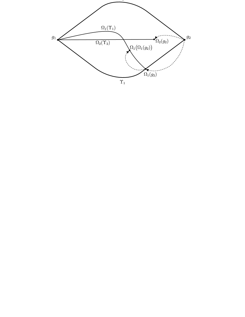
Figure 0.1: Domain $G$ with the boundary $\partial G=\bar{\Upsilon}_{1}\cup\bar{\Upsilon}_{2}$.

In this work, we will obtain necessary and sufficient condition under which problem of type (0.1), (0.2) is Fredholm. It will be shown that the solvability of such a problem is influenced by (I) spectral properties of model nonlocal problems with a parameter and (II) fulfilment of some algebraic relations between the differential operator and nonlocal boundary-value operators at the points of conjugation of nonlocal conditions (points $g_{1}$ and $g_{2}$ at Fig. 0.1). We will consider nonlocal problems both with nonhomogeneous and with homogeneous boundary-value conditions, which turn out to be not equivalent ones in terms of Fredholm solvability. Near the conjugation points, asymptotics of solutions will be obtained.

We note that nonlocal problems in Sobolev spaces in the case where the support of nonlocal terms does not intersect the boundary was thoroughly investigated by Skubachevskii [13, 17]. However, $2m$ order elliptic equations with general nonlocal conditions in the case where the support of nonlocal terms intersects the boundary is being studied in Sobolev spaces for the first time.

Our paper is organized as follows. The statement of the problem is given in Sec. 1. In the same section, we define model problems in plane angles and problems with a parameter, corresponding to the points of conjugation of nonlocal conditions. Properties of the original problem crucially depend on whether or not some line

$$\{\lambda\in\mathbb{C}:{\rm Im\,}\lambda=\Lambda\}$$ (0.3)

(where $\Lambda\in\mathbb{R}$ is defined by the order of differential equation and the order of the corresponding Sobolev spaces) contains eigenvalues of model problems with a parameter. In Sec. 2, we study nonlocal problems in plane angles in the case where the line (0.3) contains no eigenvalues, and in Sec. 3 we deal with the case where this line contains only the proper eigenvalue (see Definition 3.1). We use the results of Sec. 2 in Sec. 4 to investigate the Fredholm solvability of the original problem in a bounded domain, and in Sec. 5 to obtain an asymptotics of solutions to nonlocal problems near the conjugation points.

In [14, 16, 18], the authors consider nonlocal problems in weighted spaces $H_{a}^{l}(G)$ with the norm

$$\|u\|_{H_{a}^{k}(G)}=\left(\sum\limits_{|\alpha|\leq k}\int\limits_{G}\rho^{2(a-k+|\alpha|)}|D^{\alpha}u|^{2}\right)^{1/2}.$$

Here $k\geq 0$ is an integer, $a\in\mathbb{R}$, and $\rho=\rho(y)$ is the distance between the point $y$ and the set of conjugation points. For problem (0.1), (0.2), we have $\rho(y)={\rm dist}(y,\{g_{1},g_{2}\})$. In [16, 18], it is proved that if $f_{0}\in H_{a}^{l}(G)$, $f_{i}\in H_{a}^{l+3/2}(\Upsilon_{i})$, $a>l+1$, and the function $\{f_{0},f_{i}\}$ satisfies finitely many orthogonality conditions, then problem (0.1), (0.2) admits a solution $u\in H_{a}^{l+2}(G)$. If $a\leq l+1$, the following difficulty arises: the inclusion $u\in H_{a}^{l+2}(G)$ does not, in general, imply that $u\big{(}\Omega_{i}(y)\big{)}\big{|}_{\Upsilon_{i}}\in H_{a}^{l+3/2}(\Upsilon_{i})$. To eliminate this difficulty, one can introduce the spaces (for problem (0.1), (0.2)) with the weight function

$$\hat{\rho}(y)={\rm dist}\left(y,\big{\{}g_{1},g_{2},\Omega_{1}(g_{2}),\Omega_{1}\big{(}\Omega_{1}(g_{2})\big{)},\Omega_{2}(g_{2})\big{\}}\right)$$

and arbitrary $a\in\mathbb{R}$ and prove, in these spaces, the Fredholm solvability of nonlocal problems (see [14]). However, the presence of the weight function $\hat{\rho}(y)$ means that we impose a restriction both on the right-hand side and on the solution not only near the conjugation points $g_{1},g_{2}$ but also near the point $\Omega_{1}(g_{2})$ lying on a smooth part of the boundary and near the points $\Omega_{1}\big{(}\Omega_{1}(g_{2})\big{)}$ and $\Omega_{2}(g_{2})$ lying inside the domain (see Fig. 0.1).

In Sec. 6, we show: in spite of the fact that, for $a\leq l+1$, the inclusion $u\in H_{a}^{l+2}(G)$ does not imply the inclusion $u\big{(}\Omega_{i}(y)\big{)}\big{|}_{\Upsilon_{i}}\in H_{a}^{l+3/2}(\Upsilon_{i})$, if $a>0$, $f_{0}\in H_{a}^{l}(G)$, $f_{i}\in H_{a}^{l+3/2}(\Upsilon_{i})$, and $\{f_{0},f_{i}\}$ satisfies finitely many orthogonality conditions, then problem (0.1), (0.2) yet admits a solution $u\in H_{a}^{l+2}(G)$. In this case, as before, the line (0.3) (with $\Lambda$ depending now on the exponent $a$ as well) must not contain eigenvalues of model problems with a parameter.

In Sec. 7, with the help of the results from Sec. 3, we study nonlocal problems in bounded domains in the special case where the line (0.3) contains only a proper eigenvalue of model problems with a parameter. In this case, to provide the existence of solutions, we impose additional consistency conditions on the right-hand side at the conjugation points.

We note that the most complicated considerations in sections 4, 6, and 7 are related to constructing right regularizers for nonlocal problems in bounded domains. In all these sections, we use the same scheme to construct the regularizer, which is described in detail in Sec. 4. This allows us to dwell only on the most important moments in sections 6 and 7.

Finally, in Sec. 8, by using the results of sections 4 and 7, we obtain a criteria of Fredholm solvability of elliptic problems with homogeneous nonlocal conditions. Here algebraic relations between the differential operator and nonlocal boundary-value operators play essential role. Two examples illustrating the results of this paper are given in Sec. 9.

1 Statement of Nonlocal Problems in Bounded Domains

1.1 Statement of nonlocal problem

Let $G\subset{\mathbb{R}}^{2}$ be a bounded domain with the boundary $\partial G$. We introduce a set ${\mathcal{K}}\subset\partial G$ consisting of finitely many points and assume that $\partial G\setminus{\mathcal{K}}=\bigcup\limits_{i=1}^{N_{0}}\Upsilon_{i}$, where $\Upsilon_{i}$ are open (in the topology of $\partial G$) $C^{\infty}$-curves. In a neighborhood of each point $g\in{\mathcal{K}}$, the domain $G$ is supposed to coincide with some plane angle.

We denote by ${\bf P}(y,D_{y})$ and $B_{i\mu s}(y,D_{y})$ differential operators of orders $2m$ and $m_{i\mu}$ respectively with complex-valued $C^{\infty}$-coefficients ($i=1,\dots,N_{0};$ $\mu=1,\dots,m;$ $s=0,\dots,S_{i}$). Throughout the paper, we assume that the operator ${\bf P}(y,D_{y})$ is properly elliptic for all $y\in\bar{G}$ and the system of operators $\{B_{i\mu 0}(y,D_{y})\}_{\mu=1}^{m}$ covers ${\bf P}(y,D_{y})$ for all $i=1,\dots,N_{0}$ and $y\in\bar{\Upsilon}_{i}$ (see, e.g., [22, Ch. 2, § 1]).

For integer $k\geq 0$, we denote by $W^{k}(G)=W_{2}^{k}(G)$ the Sobolev space with the norm

$$\|u\|_{W^{k}(G)}=\left(\sum\limits_{|\alpha|\leq k}\int\limits_{G}|D^{\alpha}u|^{2}\,dy\right)^{1/2}$$

(we put $W^{0}(G)=L_{2}(G)$ for $k=0$). For integer $k\geq 1$, we introduce the space $W^{k-1/2}(\Upsilon)$ of traces on a smooth curve $\Upsilon\subset\bar{G}$, with the norm

$$\|\psi\|_{W^{k-1/2}(\Upsilon)}=\inf\|u\|_{W^{k}(G)}\quad(u\in W^{k}(G):u|_{\Upsilon}=\psi).$$ (1.1)

We consider the operators $\mathbf{P}:W^{l+2m}(G)\to W^{l}(G)$ and $\mathbf{B}_{i\mu}^{0}:W^{l+2m}(G)\to W^{l+2m-m_{i\mu}-1/2}(\Upsilon_{i})$ given by ${\bf P}u={\bf P}(y,D_{y})u$ and $\mathbf{B}_{i\mu}^{0}u=B_{i\mu 0}(y,D_{y})u(y)|_{\Upsilon_{i}}$. Hereinafter we assume that $l+2m-m_{i\mu}\geq 1$. The operators $\mathbf{P}$ and $\mathbf{B}_{i\mu}^{0}$ will correspond to a “local” boundary-value problem.

Now we proceed to define the operators corresponding to nonlocal conditions near the set $\mathcal{K}$. Let $\Omega_{is}$ ($i=1,\dots,N_{0};$ $s=1,\dots,S_{i}$) be an infinitely differentiable nondegenerate transformation mapping some neighborhood ${\mathcal{O}}_{i}$ of the curve $\overline{\Upsilon_{i}\cap\mathcal{O}_{{2\varepsilon_{0}}}(\mathcal{K})}$ onto the set $\Omega_{is}({\mathcal{O}}_{i})$ so that $\Omega_{is}(\Upsilon_{i})\subset G$ and

$$\Omega_{is}(g)\in\mathcal{K}\quad\text{for }g\in\bar{\Upsilon}_{i}\cap\mathcal{K}.$$ (1.2)

Here ${\varepsilon_{0}}>0$ and $\mathcal{O}_{{2\varepsilon_{0}}}(\mathcal{K})=\{y\in\mathbb{R}^{2}:{\rm dist}(y,\mathcal{K})<{2\varepsilon_{0}}\}$ is the $2{\varepsilon_{0}}$-neighborhood of the set $\mathcal{K}$. Thus, under the transformations $\Omega_{is}$, the curves $\Upsilon_{i}$ map strictly inside the domain $G$ while the set of end points of $\Upsilon_{i}$ maps to itself.

Let $\varepsilon_{0}$ be so small (see Remark 1.2 below) that, in the $2{\varepsilon_{0}}$-neighborhood $\mathcal{O}_{2{\varepsilon_{0}}}(g)$ of each point $g\in\mathcal{K}$, the domain $G$ coincides with a plane angle. Let us specify the structure of the transformation $\Omega_{is}$ near the set $\mathcal{K}$.

We denote by $\Omega_{is}^{+1}$ the transformation $\Omega_{is}:{\mathcal{O}}_{i}\to\Omega_{is}({\mathcal{O}}_{i})$ and by $\Omega_{is}^{-1}$ the transformation $\Omega_{is}^{-1}:\Omega_{is}({\mathcal{O}}_{i})\to{\mathcal{O}}_{i}$ being inverse to $\Omega_{is}.$ The set of all points $\Omega_{i_{q}s_{q}}^{\pm 1}(\dots\Omega_{i_{1}s_{1}}^{\pm 1}(g))\in{\mathcal{K}}$ ($1\leq s_{j}\leq S_{i_{j}},\ j=1,\dots,q$) (i.e., points which can be obtained by consecutive applying to the point $g$ the transformations $\Omega_{i_{j}s_{j}}^{+1}$ or $\Omega_{i_{j}s_{j}}^{-1}$ taking the points of ${\cal K}$ to those of ${\cal K}$) is called an orbit of $g\in{\cal K}$ and denoted by ${\rm Orb}(g)$.

Clearly, for any $g,g^{\prime}\in{\mathcal{K}}$, either ${\rm Orb}(g)={\rm Orb}(g^{\prime})$ or ${\rm Orb}(g)\cap{\rm Orb}(g^{\prime})=\varnothing$. Thus, we have ${\mathcal{K}}=\bigcup\limits_{p=1}^{N_{1}}{\rm Orb}_{p}$, where ${\rm Orb}_{p_{1}}\cap{\rm Orb}_{p_{2}}=\varnothing$ ($p_{1}\neq p_{2}$), and, for each $p=1,\dots,N_{1}$, the set ${\rm Orb}_{p}$ coincides with an orbit of some point $g\in{\mathcal{K}}$. Let each orbit ${\rm Orb}_{p}$ consist of points $g^{p}_{j}$, $j=1,\dots,N_{1p}$.

For every point $g\in\mathcal{K}$, we consider neighborhoods

$$\hat{\mathcal{V}}(g)\supset{\mathcal{V}}(g)\supset\mathcal{O}_{2\varepsilon_{0}}(g)$$ (1.3)

such that

1. in the neighborhood $\hat{\mathcal{V}}(g)$, the boundary $\partial G$ coincides with a plane angle;

2. $\overline{\hat{\mathcal{V}}(g)}\cap\overline{\hat{\mathcal{V}}(g^{\prime})}=\varnothing$ for any $g,g^{\prime}\in\mathcal{K}$, $g\neq g^{\prime}$;

3. if $g^{p}_{j}\in\bar{\Upsilon}_{i}\cap{\rm Orb}_{p}$ and $\Omega_{is}(g^{p}_{j})=g^{p}_{k},$ then ${\mathcal{V}}(g^{p}_{j})\subset\mathcal{O}_{i}$ and $\Omega_{is}\big{(}{\mathcal{V}}(g^{p}_{j})\big{)}\subset\hat{\mathcal{V}}(g^{p}_{k}).$

For each $g^{p}_{j}\in\bar{\Upsilon}_{i}\cap{\rm Orb}_{p}$, we fix an argument transformation $y\mapsto y^{\prime}(g^{p}_{j})$ which is a composition of the shift by the vector $-\overrightarrow{Og^{p}_{j}}$ and rotation by some angle so that the set ${\mathcal{V}}(g^{p}_{j})$ ($\hat{\mathcal{V}}(g^{p}_{j})$) maps onto a neighborhood ${\mathcal{V}}^{p}_{j}(0)$ ($\hat{\mathcal{V}}^{p}_{j}(0)$) of the origin while the sets $G\cap{\mathcal{V}}(g^{p}_{j})$ ($G\cap\hat{\mathcal{V}}(g^{p}_{j})$) and $\Upsilon_{i}\cap{\mathcal{V}}(g^{p}_{j})$ ($\Upsilon_{i}\cap\hat{\mathcal{V}}(g^{p}_{j})$) map to the intersection of the plane angle $K^{p}_{j}=\{y\in{\mathbb{R}}^{2}:\ r>0,\ |\omega|<b^{p}_{j}<\pi\}$ with ${\mathcal{V}}^{p}_{j}(0)$ ($\hat{\mathcal{V}}^{p}_{j}(0)$) and the intersection of a side of the angle $K^{p}_{j}$ with ${\mathcal{V}}^{p}_{j}(0)$ ($\hat{\mathcal{V}}^{p}_{j}(0)$) respectively.

Condition 1.1.

The argument transformation $y\mapsto y^{\prime}(g)$ for $y\in{\mathcal{V}}(g)$, $g\in\mathcal{K}\cap\bar{\Upsilon}_{i}$, described above reduces the transformation $\Omega_{is}(y)$ ($i=1,\dots N_{0}$, $s=1,\dots,S_{i}$) to a composition of rotation and expansion in new variables $y^{\prime}$.

Remark 1.1.

Condition 1.1 combined with the assumption that $\Omega_{is}(\Upsilon_{i})\subset G$, in particular, means that if $g\in\Omega_{is}(\bar{\Upsilon}_{i}\setminus\Upsilon_{i})\cap\bar{\Upsilon}_{j}\cap{\mathcal{K}}\neq\varnothing$, then the curves $\Omega_{is}(\bar{\Upsilon}_{i})$ and $\bar{\Upsilon}_{j}$ are nontangent to each other at the point $g$.

We introduce the bounded operators $\mathbf{B}_{i\mu}^{1}:W^{l+2m}(G)\to W^{l+2m-m_{i\mu}-1/2}(\Upsilon_{i})$ by the formula

$$\mathbf{B}_{i\mu}^{1}u=\sum\limits_{s=1}^{S_{i}}\big{(}B_{i\mu s}(y,D_{y})(\zeta u)\big{)}\big{(}\Omega_{is}(y)\big{)}\big{|}_{\Upsilon_{i}}.$$

Here $\big{(}B_{i\mu s}(y,D_{y})v\big{)}\big{(}\Omega_{is}(y)\big{)}=B_{i\mu s}(y^{\prime},D_{y^{\prime}})v(y^{\prime})|_{y^{\prime}=\Omega_{is}(y)}$ and the function $\zeta\in C^{\infty}(\mathbb{R}^{2})$ is such that

$$\zeta(y)=1\ (y\in\mathcal{O}_{{\varepsilon_{0}}/2}(\mathcal{K})),\quad\zeta(y)=0\ (y\notin\mathcal{O}_{{\varepsilon_{0}}}(\mathcal{K})).$$ (1.4)

Since $\mathbf{B}_{i\mu}^{1}u=0$ whenever ${\rm supp\,}u\subset\bar{G}\setminus\overline{\mathcal{O}_{{\varepsilon_{0}}}(\mathcal{K})}$, we say that the operator $\mathbf{B}_{i\mu}^{1}$ corresponds to nonlocal terms with the support near the set $\mathcal{K}$.

We also introduce the bounded operator $\mathbf{B}_{i\mu}^{2}:W^{l+2m}(G)\to W^{l+2m-m_{i\mu}-1/2}(\Upsilon_{i})$ satisfying the following condition.

Condition 1.2.

There exist numbers $\varkappa_{1}>\varkappa_{2}>0$ and $\rho>0$ such that, for all $u\in W^{l+2m}(G\setminus\overline{\mathcal{O}_{\varkappa_{1}}(\mathcal{K})})\cup W^{l+2m}(G_{\rho})$, the following inequalities hold:

$$\|\mathbf{B}^{2}_{i\mu}u\|_{W^{l+2m-m_{i\mu}-1/2}(\Upsilon_{i})}\leq c_{1}\|u\|_{W^{l+2m}(G\setminus\overline{\mathcal{O}_{\varkappa_{1}}(\mathcal{K})})},$$ (1.5)

$$\|\mathbf{B}^{2}_{i\mu}u\|_{W^{l+2m-m_{i\mu}-1/2}(\Upsilon_{i}\setminus\overline{\mathcal{O}_{\varkappa_{2}}(\mathcal{K})})}\leq c_{2}\|u\|_{W^{l+2m}(G_{\rho})},$$ (1.6)

where $i=1,\dots,N_{0}$; $\mu=1,\dots,m$; $c_{1},c_{2}>0$; $G_{\rho}=\{y\in G:{\rm dist}(y,\partial G)>\rho\}$.

From (1.5), it follows that $\mathbf{B}_{i\mu}^{2}u=0$ whenever ${\rm supp\,}u\subset\mathcal{O}_{\varkappa_{1}}(\mathcal{K})$. Therefore, we say that the operator $\mathbf{B}_{i\mu}^{2}$ corresponds to nonlocal terms with the support outside the set $\mathcal{K}$.

We suppose that Conditions 1.1 and 1.2 are fulfilled throughout.

Notice that we a priori assume no connection between the numbers $\varkappa_{1},\varkappa_{2},\rho$ in Condition 1.2 and the number $\varepsilon_{0}$ in Condition 1.1.

We study the following nonlocal elliptic problem:

$${\bf P}u =f_{0}(y)\quad(y\in G),$$ (1.7)

$$\mathbf{B}_{i\mu}^{0}u+\mathbf{B}_{i\mu}^{1}u+\mathbf{B}_{i\mu}^{2}u =f_{i\mu}(y)\quad(y\in\Upsilon_{i};\ i=1,\dots,N_{0};\ \mu=1,\dots,m).$$ (1.8)

Let us introduce the following operator corresponding to problem (1.7), (1.8):

$${\bf L}=\{{\bf P},\ {\bf B}_{i\mu}^{0}+{\bf B}_{i\mu}^{1}+{\bf B}_{i\mu}^{2}\}:W^{l+2m}(G)\to{\mathcal{W}}^{l}(G,\Upsilon),$$

where ${\mathcal{W}}^{l}(G,\Upsilon)=W^{l}(G)\times\prod\limits_{i=1}^{N_{0}}\prod\limits_{\mu=1}^{m}W^{l+2m-m_{i\mu}-1/2}(\Upsilon_{i})$.

Remark 1.2.

Further, we will need that $\varepsilon_{0}$ be sufficiently small (while $\varkappa_{1},\varkappa_{2},\rho$ may be arbitrary). Let us show that this does not lead to the loss of generality.

Let us have a number $\hat{\varepsilon}_{0}$ such that $0<\hat{\varepsilon}_{0}<\varepsilon_{0}$. We consider a function $\hat{\zeta}\in C^{\infty}(\mathbb{R}^{2})$ satisfying

$$\hat{\zeta}(y)=1\ (y\in\mathcal{O}_{{\hat{\varepsilon}_{0}}/2}(\mathcal{K})),\quad\hat{\zeta}(y)=0\ (y\notin\mathcal{O}_{{\hat{\varepsilon}_{0}}}(\mathcal{K}))$$

and introduce the operator $\hat{\mathbf{B}}_{i\mu}^{1}:W^{l+2m}(G)\to W^{l+2m-m_{i\mu}-1/2}(\Upsilon_{i})$ by the formula

$$\hat{\mathbf{B}}_{i\mu}^{1}u=\sum\limits_{s=1}^{S_{i}}\big{(}B_{i\mu s}(y,D_{y})(\hat{\zeta}u)\big{)}\big{(}\Omega_{is}(y)\big{)}\big{|}_{\Upsilon_{i}}.$$

Clearly, we have

$$\mathbf{B}_{i\mu}^{0}+\mathbf{B}_{i\mu}^{1}+\mathbf{B}_{i\mu}^{2}=\mathbf{B}_{i\mu}^{0}+\hat{\mathbf{B}}_{i\mu}^{1}+\hat{\mathbf{B}}_{i\mu}^{2},$$

where $\hat{\mathbf{B}}_{i\mu}^{2}=\mathbf{B}_{i\mu}^{1}-\hat{\mathbf{B}}_{i\mu}^{1}+\mathbf{B}_{i\mu}^{2}$. From example 1.1 (see Sec. 1.2), it follows that the operator $\mathbf{B}_{i\mu}^{1}-\hat{\mathbf{B}}_{i\mu}^{1}$ satisfies Condition 1.2 for some $\varkappa_{1},\varkappa_{2},\rho$. Therefore, we can always choose $\varepsilon_{0}$ being as small as necessary (maybe at the expense of the change of the operator $\mathbf{B}_{i\mu}^{2}$ and values of $\varkappa_{1},\varkappa_{2},\rho$).

1.2 Example of nonlocal problem

In the following example, we present a concrete realization for the abstract nonlocal operators $\mathbf{B}_{i\mu}^{2}$.

Example 1.1.

Let the operators ${\bf P}(y,D_{y})$ and $B_{i\mu s}(y,D_{y})$ be the same as before. Let $\Omega_{is}$ ($i=1,\ \dots,\ N_{0};$ $s=1,\ \dots,\ S_{i}$) be an infinitely differentiable nondegenerate transformation mapping some neighborhood ${\mathcal{O}}_{i}$ of the curve $\Upsilon_{i}$ onto $\Omega_{is}({\mathcal{O}}_{i})$ so that $\Omega_{is}(\Upsilon_{i})\subset G$. Notice that in this example assumption (1.2) is not necessarily supposed to hold for each $\Omega_{is}$.

We consider the following nonlocal problem:

$${\bf P}(y,D_{y})u=f_{0}(y)\quad(y\in G),$$ (1.9)

$$B_{i\mu 0}(y,D_{y})u(y)|_{\Upsilon_{i}}+\sum\limits_{s=1}^{S_{i}}\big{(}B_{i\mu s}(y,D_{y})u\big{)}\big{(}\Omega_{is}(y)\big{)}\big{|}_{\Upsilon_{i}}=f_{i\mu}(y)$$ (1.10)

$$(y\in\Upsilon_{i};\ i=1,\dots,N_{0};\ \mu=1,\dots,m).$$

Let us choose ${\varepsilon_{0}}$ so small that, for any point $g\in\mathcal{K}$, the set $\overline{\mathcal{O}_{{\varepsilon_{0}}}(g)}$ intersects with the curve $\overline{\Omega_{is}(\Upsilon_{i})}$ only if $g\in\mathcal{K}\cap\overline{\Omega_{is}(\Upsilon_{i})}$.

Let a point $g\in\mathcal{K}\cap\bar{\Upsilon}_{i}$ be such that $\Omega_{is}(g)\in\mathcal{K}$. Then we define the orbit ${\rm Orb}(g)$ of the point $g$ analogously to the above and assume that, for each point of this orbit ${\rm Orb}(g)$, Condition 1.1 holds.

Remark 1.3.

According to Remark 1.1, Condition 1.1 is a restriction upon a geometrical structure of the support of nonlocal terms near the set $\mathcal{K}$. However, if $\Omega_{is}(\bar{\Upsilon}_{i}\setminus\Upsilon_{i})\subset\partial G\setminus{\mathcal{K}}$, then we impose no restrictions upon a geometrical structure of the curve $\Omega_{is}(\bar{\Upsilon}_{i})$ near $\partial G$ (cf. [14, 16]).

We put

$${\bf P}u ={\bf P}(y,D_{y})u$$

$$\mathbf{B}_{i\mu}^{0}u =B_{i\mu 0}(y,D_{y})u(y)|_{\Upsilon_{i}},$$

$$\mathbf{B}_{i\mu}^{1}u =\sum\limits_{s=1}^{S_{i}}\big{(}B_{i\mu s}(y,D_{y})(\zeta u)\big{)}\big{(}\Omega_{is}(y)\big{)}\big{|}_{\Upsilon_{i}},$$

$$\mathbf{B}_{i\mu}^{2}u =\sum\limits_{s=1}^{S_{i}}\big{(}B_{i\mu s}(y,D_{y})((1-\zeta)u)\big{)}\big{(}\Omega_{is}(y)\big{)}\big{|}_{\Upsilon_{i}},$$

where $\zeta$ is defined by (1.4) (see figures 1.1 and 1.2). Then problem (1.9), (1.10) assumes the form (1.7), (1.8).

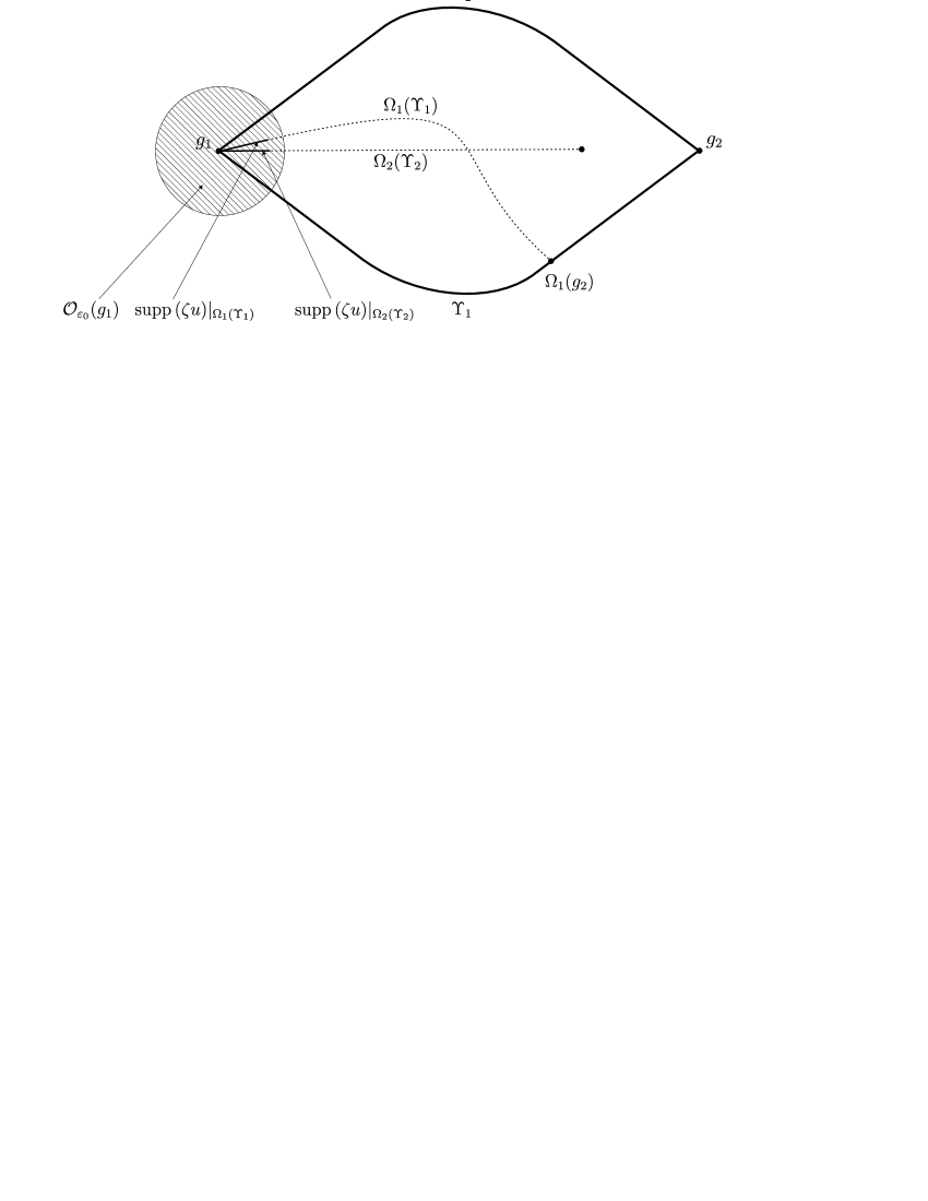
Figure 1.1: Dotted lines denote the support of nonlocal terms corresponding to the operator $\mathbf{B}_{i\mu}^{2}$.

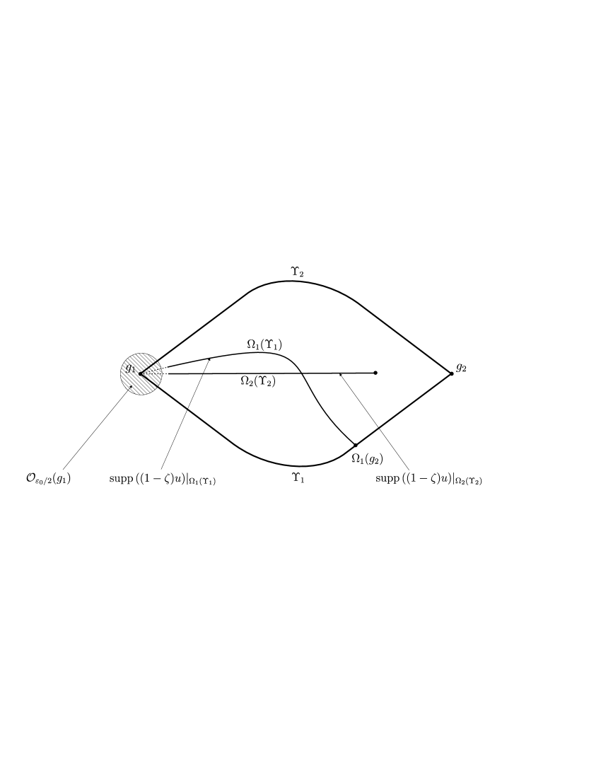
Figure 1.2: Dotted lines denote the support of nonlocal terms corresponding to the operator $\mathbf{B}_{i\mu}^{1}$.

Analogously to the proof of Lemma 2.5 [16] (where weighted spaces should be replaced by corresponding Sobolev spaces), one can show that the operator $\mathbf{B}_{i\mu}^{2}$ satisfies Condition 1.2. Let us prove, for example, inequality (1.5). Clearly, it suffices to consider an arbitrary term $\psi=\big{(}B_{i\mu s}(y,D_{y})((1-\zeta)u)\big{)}\big{(}\Omega_{is}(y)\big{)}\big{|}_{\Upsilon_{i}}$. We introduce a function $v\in C_{0}^{\infty}\big{(}\Omega_{is}({\mathcal{O}}_{i})\big{)}$ such that

$$v|_{\Omega_{is}(\Upsilon_{i})}=\big{(}B_{i\mu s}(y,D_{y})((1-\zeta)u)\big{)}\big{|}_{\Omega_{is}(\Upsilon_{i})},$$ (1.11)

$$\|v\|_{W^{l+2m-m_{i\mu}}(\Omega_{is}({\mathcal{O}}_{i}))}\leq 2\big{\|}\big{(}B_{i\mu s}(y,D_{y})((1-\zeta)u)\big{)}\big{|}_{\Omega_{is}(\Upsilon_{i})}\big{\|}_{W^{l+2m-m_{i\mu}-1/2}(\Omega_{is}(\Upsilon_{i}))},$$ (1.12)

From (1.11), it follows that

$$v\big{(}\Omega_{is}(y)\big{)}\big{|}_{\Upsilon_{i}}=\psi.$$

Combining this with the boundedness of the trace operator in Sobolev spaces and inequality (1.12), we get

$$\|\psi\|_{W^{l+2m-m_{i\mu}-1/2}(\Upsilon_{i})}=\big{\|}v\big{(}\Omega_{is}(y)\big{)}\big{|}_{\Upsilon_{i}}\big{\|}_{W^{l+2m-m_{i\mu}-1/2}(\Upsilon_{i})}\leq\left\|v\big{(}\Omega_{is}(y)\big{)}\right\|_{W^{l+2m-m_{i\mu}}(\mathcal{O}_{i})}\\ \leq k_{1}\|v\|_{W^{l+2m-m_{i\mu}}(\Omega_{is}(\mathcal{O}_{i}))}\leq 2k_{1}\|B_{i\mu s}(y,D_{y})((1-\zeta)u)|_{\Upsilon_{i}}\|_{W^{l+2m-m_{i\mu}-1/2}(\Omega_{is}(\Upsilon_{i}))}\\ \leq k_{2}\|(1-\zeta)u\|_{W^{l+2m}(G)}.$$ (1.13)

Thus, putting $\varkappa_{1}={\varepsilon_{0}}/2$, we see that (1.13) implies estimate (1.5). Notice that, in this case, the numbers $\varkappa_{1}$ and ${\varepsilon_{0}}$ turn out to be connected with each other.

Analogous considerations allow one to obtain estimate (1.6). The proof is based on the boundedness of the trace operator, smoothness of the transformations $\Omega_{is}$, and relation

$$\Omega_{is}(\Upsilon_{i}\setminus\overline{\mathcal{O}_{\varkappa_{2}}(\mathcal{K})})\subset G_{\rho}$$

(which is valid for any $\varkappa_{2}<\varkappa_{1}$ and sufficiently small $\rho=\rho(\varkappa_{2})$). The latter relation follows from the embedding $\Omega_{is}(\Upsilon_{i})\subset G$ and continuity of $\Omega_{is}$.

1.3 Nonlocal problems near the set $\mathcal{K}$

While studying problem (1.7), (1.8), one must pay especial attention to a behavior of solutions in a neighborhood of the set ${\mathcal{K}}$, which consists of the conjugation points. Let us consider corresponding model problems in plane angles. To this end, we formally assume that

$${\mathbf{B}}_{i\mu}^{2}=0,\quad i=1,\dots,N_{0},\ \mu=1,\dots,m.$$ (1.14)

Let us fix some orbit ${\rm Orb}_{p}\subset{\mathcal{K}}$ ($p=1,\dots,N_{1}$) and suppose that ${\rm supp\,}u\subset\Big{(}\bigcup\limits_{j=1}^{N_{1p}}{\mathcal{V}}(g^{p}_{j})\Big{)}\cap\bar{G}.$ We denote by $u_{j}(y)$ the function $u(y)$ for $y\in\hat{\mathcal{V}}(g^{p}_{j})\cap G$. If $g^{p}_{j}\in\bar{\Upsilon}_{i},$ $y\in{\mathcal{V}}(g^{p}_{j})$, and $\Omega_{is}(y)\in\hat{\mathcal{V}}(g^{p}_{k}),$ we denote $u(\Omega_{is}(y))$ by $u_{k}(\Omega_{is}(y))$. Then, by virtue of assumption (1.14), nonlocal problem (1.7), (1.8) assumes the following form:

$${\bf P}(y,D_{y})u_{j}=f_{0}(y)\quad(y\in{\mathcal{V}}(g^{p}_{j})\cap G),$$

$$\begin{aligned} B_{i\mu 0}(y,D_{y})u_{j}(y)|_{{\mathcal{V}}(g^{p}_{j})\cap\Upsilon_{i}}+\sum\limits_{s=1}^{S_{i}}\big{(}B_{i\mu s}(y,D_{y})(\zeta u_{k})\big{)}\big{(}\Omega_{is}(y)\big{)}\big{|}_{{\mathcal{V}}(g^{p}_{j})\cap\Upsilon_{i}}=f_{i\mu}(y)\\ \big{(}y\in{\mathcal{V}}(g^{p}_{j})\cap\Upsilon_{i};\ i\in\{1\leq i\leq N_{0}:g^{p}_{j}\in\bar{\Upsilon}_{i}\};\ j=1,\dots,N_{1p};\ \mu=1,\dots,m\big{)}.\end{aligned}$$

Let $y\mapsto y^{\prime}(g^{p}_{j})$ be the argument transformation described above. We introduce the function $U_{j}(y^{\prime})=u_{j}(y(y^{\prime}))$ and denote $y^{\prime}$ again by $y$. For $p$ being fixed, we put $N=N_{1p}$, $b_{j}=b^{p}_{j}$, $K_{j}=K^{p}_{j}$ (see Sec. 1.1), and $\gamma_{j\sigma}=\{y\in{\mathbb{R}}^{2}:r>0,\ \omega=(-1)^{\sigma}b_{j}\}$ ($\sigma=1,2$), where $(\omega,r)$ are polar coordinates with pole at the origin. Now, using Condition 1.1, we can rewrite problem (1.7), (1.8) as follows:

$${\bf P}_{j}(y,D_{y})U_{j}=f_{j}(y)\quad(y\in K_{j}),$$ (1.15)

$${\bf B}_{j\sigma\mu}(y,D_{y})U|_{\gamma_{j\sigma}}\equiv\sum\limits_{k,s}(B_{j\sigma\mu ks}(y,D_{y})U_{k})({\mathcal{G}}_{j\sigma ks}y)|_{\gamma_{j\sigma}}=f_{j\sigma\mu}(y)\quad(y\in\gamma_{j\sigma}).$$ (1.16)

Here (and further, unless the contrary is specified) $j,k=1,\dots,N=N_{1p};$ $\sigma=1,2;$ $\mu=1,\dots,m;$ $s=0,\dots,S_{j\sigma k}$; ${\mathbf{P}}_{j}(y,D_{y})$ and $B_{j\sigma\mu ks}(y,D_{y})$ are operators of orders $2m$ and $m_{j\sigma\mu}$ respectively with variable $C^{\infty}$-coefficients; ${\mathcal{G}}_{j\sigma ks}$ is the operator of rotation by an angle $\omega_{j\sigma ks}$ and expansion $\chi_{j\sigma ks}$ ($\chi_{j\sigma ks}>0$) times in $y$-plane. Furthermore, $|(-1)^{\sigma}b_{j}+\omega_{j\sigma ks}|<b_{k}$ for $(j,0)\neq(k,s)$, $\omega_{j\sigma j0}=0$, and $\chi_{j\sigma j0}=1$.

Since $\mathcal{V}(0)\supset\mathcal{O}_{\varepsilon_{0}}(0)$ (see. (1.3)), it follows that, for any function $v$ (which need not be compactly supported), we have

$$B_{j\sigma\mu ks}(y,D_{y})v(y)=0\quad\text{for }|y|\geq\varepsilon_{0},\ (k,s)\neq(j,0).$$ (1.17)

Moreover, since we consider problem (1.15), (1.16) for functions $U$ with compact support, we may assume that the coefficients of the operators ${\bf P}_{j}(y,D_{y})$ and $B_{j\sigma\mu j0}(y,D_{y})$ are equal to zero outside a disk of sufficiently large radius.

Let us introduce the following spaces of vector-functions:

$$W^{l+2m,N}(K)=\prod_{j=1}^{N}W^{l+2m}(K_{j}),\ \mathcal{W}^{l,N}(K,\gamma)=\prod_{j=1}^{N}{\mathcal{W}}^{l}(K_{j},\gamma_{j}),$$

$${\mathcal{W}}^{l}(K_{j},\gamma_{j})=W^{l}(K_{j})\times\prod\limits_{\sigma=1,2}\prod\limits_{\mu=1}^{m}W^{l+2m-m_{j\sigma\mu}-1/2}(\gamma_{j\sigma}).$$

We consider the operator ${\bf L}_{p}:W^{l+2m,N}(K)\to\mathcal{W}^{l,N}(K,\gamma)$ given by

$${\bf L}_{p}U=\{{\bf P}_{j}(y,D_{y})U_{j},\ {\bf B}_{j\sigma\mu}(y,D_{y})U|_{\gamma_{j\sigma}}\}$$

and corresponding to problem (1.15), (1.16). Subindex $p$ means that the operator ${\bf L}_{p}$ is related to the orbit ${\rm Orb}_{p}$.

We denote by ${\mathcal{P}}_{j}(D_{y})$ and $B_{j\sigma\mu ks}(D_{y})$ the principal homogeneous parts of the operators ${\bf P}_{j}(0,D_{y})$ and $B_{j\sigma\mu ks}(0,D_{y})$ respectively. Along with problem (1.15), (1.16), we study the model nonlocal problem

$${\mathcal{P}}_{j}(D_{y})U_{j}=f_{j}(y)\quad(y\in K_{j}),$$ (1.18)

$${\mathcal{B}}_{j\sigma\mu}(D_{y})U|_{\gamma_{j\sigma}}\equiv\sum\limits_{k,s}(B_{j\sigma\mu ks}(D_{y})U_{k})({\mathcal{G}}_{j\sigma ks}y)|_{\gamma_{j\sigma}}=f_{j\sigma\mu}(y)\quad(y\in\gamma_{j\sigma}).$$ (1.19)

We introduce the operator ${\mathcal{L}}_{p}:W^{l+2m,N}(K)\to\mathcal{W}^{l,N}(K,\gamma)$ given by

$${\mathcal{L}}_{p}U=\{{\mathcal{P}}_{j}(D_{y})U_{j},\ {\mathcal{B}}_{j\sigma\mu}(D_{y})U|_{\gamma_{j\sigma}}\}$$

and corresponding to problem (1.18), (1.19).

Let us write the operators ${\mathcal{P}}_{j}(D_{y})$ and $B_{j\sigma\mu ks}(D_{y})$ in polar coordinates: ${\mathcal{P}}_{j}(D_{y})=r^{-2m}\tilde{\mathcal{P}}_{j}(\omega,D_{\omega},rD_{r}),$ $B_{j\sigma\mu ks}(D_{y})=r^{-m_{j\sigma\mu}}\tilde{B}_{j\sigma\mu ks}(\omega,D_{\omega},rD_{r})$.

We introduce the spaces of vector-functions

$$W^{l+2m,N}(-b,b)=\prod_{j=1}^{N}W^{l+2m}(-b_{j},b_{j}),\ \mathcal{W}^{l,N}[-b,b]=\prod_{j=1}^{N}{\mathcal{W}}^{l}[-b_{j},b_{j}],$$

$${\mathcal{W}}^{l}[-b_{j},b_{j}]=W^{l}(-b_{j},b_{j})\times{\mathbb{C}}^{2m}$$

and consider the analytic operator-valued function $\tilde{\mathcal{L}}_{p}(\lambda):W^{l+2m,N}(-b,b)\to{\mathcal{W}}^{l,N}[-b,b]$ given by

$$\tilde{\mathcal{L}}_{p}(\lambda)\varphi=\{\tilde{\mathcal{P}}_{j}(\omega,D_{\omega},\lambda)\varphi_{j},\ \sum\limits_{k,s}(\chi_{j\sigma ks})^{i\lambda-m_{j\sigma\mu}}{\tilde{B}}_{j\sigma\mu ks}(\omega,D_{\omega},\lambda)\varphi_{k}(\omega+\omega_{j\sigma ks})|_{\omega=(-1)^{\sigma}b_{j}}\}.$$

Main definitions and facts concerning eigenvalues, eigenvectors, and associate vectors of analytic operator-valued functions can be found in [23]. In the sequel, it will be on principle that the spectrum of the operator $\tilde{\mathcal{L}}_{p}(\lambda)$ is discrete (see Lemma 2.1 [15]).

Further, we will show that the Fredholm solvability of problem (1.7), (1.8) in Sobolev spaces depends on the location of eigenvalues of model operators $\tilde{\mathcal{L}}_{p}(\lambda)$ corresponding to the points of ${\mathcal{K}}$. Notice that the solvability of the same problem in weighted spaces depends on the location of eigenvalues of model operators corresponding not only to the points of ${\mathcal{K}}$ but also $\Omega_{is}({\mathcal{K}})\subset\bar{G}$ and $\Omega_{i^{\prime}s^{\prime}}(\Omega_{is}({\mathcal{K}})\cap\Upsilon_{i^{\prime}})\subset G$ (see [14, 16]). This can be explained as follows: the points of the sets indicated are connected by means of the transformations $\Omega_{is}$. That is why singularities of solutions appearing near the set ${\mathcal{K}}$ may be “carried” to other points both on the boundary and strictly inside the domain. But in our case we will prove that if the right-hand side of problem (1.7), (1.8) is subject to finitely many orthogonality conditions in the Sobolev space ${\mathcal{W}}^{l}(G,\Upsilon)$, then the solutions belong to the Sobolev space $W^{l+2m}(G)$. Therefore, such solutions have no singularities.

2 Nonlocal Problems in Plane Angles in the Case where the Line ${\rm Im\,}\lambda=1-l-2m$ Contains no Eigenvalues of $\tilde{\mathcal{L}}_{p}(\lambda)$

In this section, we construct an operator acting in Sobolev spaces, defined for compactly supported functions, and being the right inverse for the operator ${\bf L}_{p}$ up to the sum of small and compact perturbations. (We remind that ${\bf L}_{p}$ corresponds to model problem (1.15), (1.16).)

2.1 Weighted spaces $H_{a}^{k}(Q)$

Throughout this section, we suppose that the orbit ${\rm Orb}_{p}$ is fixed; therefore, for short, we denote the operators ${\bf L}_{p}$, $\mathcal{L}_{p}$, and $\tilde{\mathcal{L}}_{p}(\lambda)$ by ${\mathfrak{L}}$, $\mathcal{L}$, and $\tilde{\mathcal{L}}(\lambda)$ respectively.

The investigation of the solvability for problem (1.15), (1.16) in Sobolev spaces will be based upon the results on the solvability of problem (1.18), (1.19) in weighted spaces. Let us introduce these spaces and present some of their properties.

For any set $X\in\mathbb{R}^{n}$ ($n\geq 1$), we denote by $C_{0}^{\infty}(X)$ the set of functions infinitely differentiable in $\bar{X}$ and compactly supported in $X$. Let either $Q=K_{j}$ or $Q=K_{j}\cap\{y\in\mathbb{R}^{2}:\ |y|<d\}\ (d>0)$, or $Q={\mathbb{R}}^{2}$. Denote by $H_{a}^{k}(Q)$ the completion of the set $C_{0}^{\infty}(\bar{Q}\setminus\{0\})$ with respect to the norm

$$\|w\|_{H_{a}^{k}(Q)}=\left(\sum_{|\alpha|\leq k}\int\limits_{Q}r^{2(a-k+|\alpha|)}|D_{y}^{\alpha}w|^{2}dy\right)^{1/2},$$

where $a\in\mathbb{R}$, $k\geq 0$ is an integer. For $k\geq 1$, we denote by $H_{a}^{k-1/2}(\gamma)$ the space of traces on a smooth curve $\gamma\subset\bar{Q}$ with the norm

$$\|\psi\|_{H_{a}^{k-1/2}(\gamma)}=\inf\|w\|_{H_{a}^{k}(Q)}\quad(w\in H_{a}^{l}(Q):w|_{\gamma}=\psi).$$

We introduce the following spaces of vector-functions:

$$\begin{matrix}H_{a}^{l+2m,N}(K)=\prod\limits_{j=1}^{N}H_{a}^{l+2m}(K_{j}),\ \mathcal{H}_{a}^{l,N}(K,\gamma)=\prod\limits_{j=1}^{N}\mathcal{H}_{a}^{l}(K_{j},\gamma_{j}),\\ \mathcal{H}_{a}^{l}(K_{j},\gamma_{j})=H_{a}^{l}(K_{j})\times\prod\limits_{\sigma=1,2}\prod\limits_{\mu=1}^{m}H_{a}^{l+2m-m_{j\sigma\mu}-1/2}(\gamma_{j\sigma}).\end{matrix}$$

The bounded operator ${\mathcal{L}}_{a}:H_{a}^{l+2m,N}(K)\to\mathcal{H}_{a}^{l,N}(K,\gamma)$ given by

$${\mathcal{L}}_{a}U=\{{\mathcal{P}}_{j}(D_{y})U_{j},\ {\mathcal{B}}_{j\sigma\mu}(D_{y})U|_{\gamma_{j\sigma}}\}$$ (2.1)

corresponds to problem (1.18), (1.19) in the weighted spaces. From Theorem 2.1 [15], it follows that the operator ${\mathcal{L}}_{a}$ has a bounded inverse if and only if the line ${\rm Im\,}\lambda=1-l-2m$ contains no eigenvalues of the operator $\tilde{\mathcal{L}}(\lambda)$. Using the invertibility of ${\mathcal{L}}_{a}$, in this section and next one, we will study the solvability of problems (1.18), (1.19) and (1.15), (1.16) in Sobolev spaces. To this end, we need some auxiliary results (Lemmas 2.1 and 2.2) concerning the relation between the spaces $H_{a}^{k}(\cdot)$ and $W^{k}(\cdot)$.

Lemma 2.1.

Let $u\in W^{k}(Q)$ ($k\geq 2$), $u(y)=0$ for $|y|\geq 1$, and $D^{\alpha}u|_{y=0}=0$ ($|\alpha|\leq k-2$). Then we have

$$\|u\|_{H_{a}^{k}(Q)}\leq c_{a}\|u\|_{W^{k}(Q)},\quad a>0.$$ (2.2)

If we additionally suppose that $D^{k-1}u\in H_{0}^{1}(Q)$, then we have

$$\|u\|_{H_{0}^{k}(Q)}\leq c\sum\limits_{|\alpha|=k-1}\|D^{\alpha}u\|_{H_{0}^{1}(Q)}.$$ (2.3)

Here $Q$ is the same domain as before, $c_{a}>0$ is independent of $u$.

Proof.

From Lemma 4.9 [21], it follows that, for each $a>0$,

$$\|D^{k-1}u\|_{H_{a}^{1}(Q)}\leq c\|D^{k-1}u\|_{W^{1}(Q)}\leq c\|u\|_{W^{k}(Q)}.$$

Combining this estimate (or the inclusion $D^{k-1}u\in H_{0}^{1}(Q)$) with Lemma 4.12 [21] yields inequality (2.2) for $0<a<1$ (or inequality (2.3) respectively). Since the support of $u$ is compact, it follows that inequality (2.2) holds for all $a>0$. ∎

Lemma 2.2.

Let $u\in W^{1}({\mathbb{R}}^{2})$ and $u(y)=0$ for $|y|\geq 1$. Then we have

$$\|u(y)-u({\mathcal{G}}_{0}y)\|_{H_{0}^{1}({\mathbb{R}}^{2})}\leq c\|u\|_{W^{1}({\mathbb{R}}^{2})},$$

where ${\mathcal{G}}_{0}$ is a composition of rotation by an angle $\omega_{0}$ ($-\pi<\omega_{0}\leq\pi$) and expansion $\chi_{0}$ ($\chi_{0}>0$) times.

Proof.

Writing a function $u$ in polar coordinates $(\omega,r)$ yields

$$u(y)-u({\mathcal{G}}_{0}y)=u(\omega,r)-u(\omega+\omega_{0},\chi_{0}r)=v_{1}+v_{2},$$

where $v_{1}(\omega,r)=u(\omega,r)-u(\omega+\omega_{0},r)$, $v_{2}(\omega,r)=u(\omega+\omega_{0},r)-u(\omega+\omega_{0},\chi_{0}r)$.

Let us consider the function $v_{1}$. By Lemma 4.15 [21], we obtain

$$\int\limits_{0}^{\infty}r^{-1}|v_{1}(0,r)|^{2}dr\leq k_{1}\|u\|_{W^{1}({\mathbb{R}}^{2})}.$$

From this and Lemma 4.8 [21], it follows that $v_{1}\in H_{0}^{1}({\mathbb{R}}^{2})$ and

$$\|v_{1}\|_{H_{0}^{1}({\mathbb{R}}^{2})}\leq k_{2}\|u\|_{W^{1}({\mathbb{R}}^{2})}.$$ (2.4)

To prove the lemma, it remains to show that

$$\int\limits_{{\mathbb{R}}^{2}}r^{-2}|v_{2}|^{2}dy\leq k_{3}\|u\|_{W^{1}({\mathbb{R}}^{2})}.$$ (2.5)

For $\chi_{0}>1$ (the case where $0<\chi_{0}<1$ can be considered analogously), we have

$$\int\limits_{{\mathbb{R}}^{2}}r^{-2}|v_{2}|^{2}dy=\int\limits_{-\pi}^{\pi}d\omega\int\limits_{0}^{\infty}r^{-1}|v_{2}(\omega,r)|^{2}dr=\int\limits_{-\pi+\omega_{0}}^{\pi+\omega_{0}}d\omega\int\limits_{0}^{\infty}r^{-1}dr\left|\int\limits_{r}^{\chi_{0}r}\frac{\partial u(\omega,t)}{\partial t}dt\right|^{2}.$$

Using the Schwarz inequality, followed by the change of integration limits, we get estimate (2.5):

$$\int\limits_{\mathbb{R}^{2}}r^{-2}|v_{2}|^{2}dy\leq(\chi_{0}-1)\int\limits_{-\pi+\omega_{0}}^{\pi+\omega_{0}}d\omega\int\limits_{0}^{\infty}dr\int\limits_{r}^{\chi_{0}r}\left|\frac{\partial u(\omega,t)}{\partial t}\right|^{2}dt\\ =\frac{(\chi_{0}-1)^{2}}{\chi_{0}}\int\limits_{-\pi+\omega_{0}}^{\pi+\omega_{0}}d\omega\int\limits_{0}^{\infty}\left|\frac{\partial u(\omega,t)}{\partial t}\right|^{2}t\,dt\leq\frac{(\chi_{0}-1)^{2}}{\chi_{0}}\|u\|^{2}_{W^{1}({\mathbb{R}}^{2})}.$$ (2.6)

∎

Let us prove one more auxiliary result.

Lemma 2.3.

Let $H,\ H_{1},$ and $H_{2}$ be Hilbert spaces, ${\mathfrak{A}}:H\to H_{1}$ a linear bounded operator, and ${\cal T}:H\to H_{2}$ a compact operator. Suppose that, for some $\varepsilon>0,\ c>0$, and $f\in H$, the following inequality holds:

$$\|{\mathfrak{A}}f\|_{H_{1}}\leq\varepsilon\|f\|_{H}+c\|{\cal T}f\|_{H_{2}}.$$ (2.7)

Then there exist operators ${\cal M},{\cal F}:H\to H_{1}$ such that

$${\mathfrak{A}}={\cal M}+{\cal F},$$

$\|{\cal M}\|\leq 2\varepsilon$, and the operator ${\cal F}$ is finite-dimensional.

Proof.

As is well known (see, e.g., [24, Ch. 5, § 85]), any compact operator is the limit of a uniformly convergent sequence of finite-dimensional operators. Therefore, there exist bounded operators ${\cal M}_{0},{\cal F}_{0}:H\to H_{2}$ such that ${\cal T}={\cal M}_{0}+{\cal F}_{0}$, $\|{\cal M}_{0}\|\leq c^{-1}\varepsilon$, and the operator ${\cal F}_{0}$ is finite-dimensional. This and (2.7) imply

$$\|{\mathfrak{A}}f\|_{H_{1}}\leq 2\varepsilon\|f\|_{H}+c\|{\cal F}_{0}f\|_{H_{2}}\quad\mbox{for all }f\in H.$$ (2.8)

Denote by ${\rm ker\,}({\cal F}_{0})^{\bot}$ the orthogonal supplement in $H$ to the kernel of the operator ${\cal F}_{0}$. Since the finite-dimensional operator ${\cal F}_{0}$ maps ${\rm ker\,}({\cal F}_{0})^{\bot}$ onto its image in a one-to-one manner, the subspace ${\rm ker\,}({\cal F}_{0})^{\bot}$ is of finite dimension. Let ${\cal I}$ denote the identity operator in $H$ and ${\cal P}_{0}$ the orthogonal projector onto ${\rm ker\,}({\cal F}_{0})^{\bot}$. Clearly, ${\mathfrak{A}}{\cal P}_{0}:H\to H_{1}$ is a finite-dimensional operator. Furthermore, since ${\cal I}-{\cal P}_{0}$ is the orthogonal projector onto ${\rm ker\,}({\cal F}_{0})$, it follows that ${\cal F}_{0}({\cal I}-{\cal P}_{0})=0$. Therefore, substituting the function $({\cal I}-{\cal P}_{0})f$ instead of $f$ in (2.8), we get

$$\|{\mathfrak{A}}({\cal I}-{\cal P}_{0})f\|_{H_{1}}\leq 2\varepsilon\|({\cal I}-{\cal P}_{0})f\|_{H}\leq 2\varepsilon\|f\|_{H}\quad\text{for all }f\in H.$$

Denoting ${\cal M}={\mathfrak{A}}({\cal I}-{\cal P}_{0})$ and ${\cal F}={\mathfrak{A}}{\cal P}_{0}$ completes the proof. ∎

2.2 Construction of the operator $\mathfrak{R}$

In this subsection, we construct the operator $\mathfrak{R}$ acting in a subspace $\mathcal{S}^{l,N}(K,\gamma)$ of the space $W^{l,N}(K,\gamma)$, defined for compactly supported functions, and being the right inverse for the operator $\mathfrak{L}$ up to the sum of small and compact perturbations (see Theorem 2.1). To construct such an operator, we assume that the following condition holds.

Condition 2.1.

The line ${\rm Im\,}\lambda=1-l-2m$ contains no eigenvalues of the operator $\tilde{\mathcal{L}}(\lambda)$.

We denote by $\mathcal{S}^{l,N}(K,\gamma)$ the subspace of $\mathcal{W}^{l,N}(K,\gamma)$, consisting of the functions $\{f_{j},f_{j\sigma\mu}\}$ such that

$$D^{\alpha}f_{j}|_{y=0}=0,\quad|\alpha|\leq l-2,$$ (2.9)

$$\left.\frac{\partial^{\beta}f_{j\sigma\mu}}{\partial\tau_{j\sigma}^{\beta}}\right|_{y=0}=0,\quad\beta\leq l+2m-m_{j\sigma\mu}-2,$$ (2.10)

where $\tau_{j\sigma}$ is the unit vector directed along the ray $\gamma_{j\sigma}$. If $l-2<0$ or $l+2m-m_{j\sigma\mu}-2<0$, the corresponding conditions are absent. From Sobolev’s embedding theorem and Riesz’ theorem on a general form of linear continuous functionals in Hilbert spaces, it follows that the set $\mathcal{S}^{l,N}(K,\gamma)$ is closed and of finite codimension in $\mathcal{W}^{l,N}(K,\gamma)$.

Let us consider the operators

$$\frac{\partial^{l+2m-m_{j\sigma\mu}-1}}{\partial\tau_{j\sigma}^{l+2m-m_{j\sigma\mu}-1}}{\mathcal{B}}_{j\sigma\mu}(D_{y})U\equiv\frac{\partial^{l+2m-m_{j\sigma\mu}-1}}{\partial\tau_{j\sigma}^{l+2m-m_{j\sigma\mu}-1}}\Big{(}\sum\limits_{k,s}(B_{j\sigma\mu ks}(D_{y})U_{k})({\mathcal{G}}_{j\sigma ks}y)\Big{)}.$$

Using the chain rule, we can write

$$\frac{\partial^{l+2m-m_{j\sigma\mu}-1}}{\partial\tau_{j\sigma}^{l+2m-m_{j\sigma\mu}-1}}{\mathcal{B}}_{j\sigma\mu}(D_{y})U\equiv\sum\limits_{k,s}(\hat{B}_{j\sigma\mu ks}(D_{y})U_{k})({\mathcal{G}}_{j\sigma ks}y),$$ (2.11)

where $\hat{B}_{j\sigma\mu ks}(D_{y})$ are some homogenous differential operators of order $l+2m-1$ with constant coefficients. In particular, we have $\hat{B}_{j\sigma\mu j0}(D_{y})=\dfrac{\partial^{l+2m-m_{j\sigma\mu}-1}}{\partial\tau_{j\sigma}^{l+2m-m_{j\sigma\mu}-1}}B_{j\sigma\mu j0}(D_{y})$ since ${\mathcal{G}}_{j\sigma j0}y\equiv y$. Formally replacing the nonlocal operators in (2.11) by the corresponding local ones, we introduce the operators

$$\hat{\mathcal{B}}_{j\sigma\mu}(D_{y})U\equiv\sum\limits_{k,s}\hat{B}_{j\sigma\mu ks}(D_{y})U_{k}(y).$$ (2.12)

Along with system (2.12), we consider (for $l\geq 1$) the operators

$$D^{\xi}{\mathcal{P}}_{j}(D_{y})U_{j}(y),\quad|\xi|=l-1.$$ (2.13)

The system of operators (2.12) and (2.13) plays an essential in the proof of the following lemma, which is used for the construction of the operator $\mathfrak{R}$.

Lemma 2.4.

Let Condition 2.1 hold. Then, for any $\varepsilon$, $0<\varepsilon<1$, there exists a bounded operator

$$\mathcal{A}:\{f\in\mathcal{S}^{l,N}(K,\gamma):{\rm supp\,}f\subset\mathcal{O}_{\varepsilon}(0)\}\to W^{l+2m,N}(K)$$

such that, for any $f=\{f_{j},f_{j\sigma\mu}\}\in{\rm Dom}(\mathcal{A})$, the function $V=\mathcal{A}f$ satisfies the following conditions: $V=0$ for $|y|\geq 1$,

$$\|{\mathcal{L}}V-f\|_{\mathcal{H}_{0}^{l,N}(K)}\leq c\|f\|_{\mathcal{W}^{l,N}(K,\gamma)},$$ (2.14)

$$\|V\|_{H_{a}^{l+2m,N}(K)}\leq c_{a}\|f\|_{\mathcal{W}^{l,N}(K,\gamma)}\quad\mbox{for any}\ a>0.$$ (2.15)

Proof.

1. We introduce the operator

$$f_{j\sigma\mu}\mapsto\Phi_{j\sigma\mu}$$ (2.16)

taking a function $f_{j\sigma\mu}\in W^{l+2m-m_{j\sigma\mu}-1/2}(\gamma_{j\sigma})$ to its extension $\Phi_{j\sigma\mu}\in W^{l+2m-m_{j\sigma\mu}}({\mathbb{R}}^{2})$ to ${\mathbb{R}}^{2}$, satisfying $\Phi_{j\sigma\mu}=0$ for $|y|\geq 2$. We also consider an extension of the function $f_{j}$ from $K_{j}$ to ${\mathbb{R}}^{2}$ so that the extended function (which we also denote by $f_{j}$) is equal to zero for $|y|\geq 2$. The corresponding extension operators can be chosen linear and bounded (see [25, Ch. 6, § 3]).

Let us consider the following linear algebraic system for all partial derivatives $D^{\alpha}W_{j}$, $|\alpha|=l+2m-1$, $j=1,\dots,N$:

$$\hat{\mathcal{B}}_{j\sigma\mu}(D_{y})W=\frac{\partial^{l+2m-m_{j\sigma\mu}-1}}{\partial\tau_{j\sigma}^{l+2m-m_{j\sigma\mu}-1}}\Phi_{j\sigma\mu},$$ (2.17)

$$D^{\xi}\mathcal{P}_{j}(D_{y})W_{j}=D^{\xi}f_{j}$$ (2.18)

($j=1,\dots,N$; $\sigma=1,2$; $\mu=1,\dots,m$; $|\xi|=l-1$). We remind that each of the operators $\hat{\mathcal{B}}_{j\sigma\mu}(D_{y})$ given by (2.12) is the sum of “local” operators, which allows us to regard system (2.17), (2.18) as an algebraic one. Let us take for granted that system (2.17), (2.18) admits a unique solution for any right-hand side. Denote by $W_{j\alpha}$ a solution of system (2.17), (2.18). It is obvious that $W_{j\alpha}\in W^{1}(\mathbb{R}^{2})$ and $W_{j\alpha}=0$ for $|y|\geq 2$. By virtue of Lemma 4.17 [21], there exists a linear bounded operator

$$\{W_{j\alpha}\}_{|\alpha|=l+2m-1}\mapsto V_{j}$$ (2.19)

taking a system $\{W_{j\alpha}\}_{|\alpha|=l+2m-1}\in\prod\limits_{|\alpha|=l+2m-1}W^{1}(\mathbb{R}^{2})$ to a function $V_{j}\in W^{l+2m}(\mathbb{R}^{2})$ such that $V_{j}(y)=0$ for $|y|\geq 1$,

$$D^{\alpha}V_{j}|_{y=0}=0,\quad|\alpha|\leq l+2m-2,$$ (2.20)

$$D^{\alpha}V_{j}-W_{j\alpha}\in H_{0}^{1}(\mathbb{R}^{2}),\quad|\alpha|=l+2m-1.$$ (2.21)

2. Let us show that the function $V=(V_{1},\dots,V_{N})$ is that we are seeking for. Inequality (2.15) follows from relations (2.20), Lemma 2.1, and the boundedness of the operator (2.19).

Let us prove (2.14). Since the functions $W_{j\alpha}$ are solutions of algebraic system (2.17), (2.18) and the functions $V_{j}$ satisfy (2.21), it follows that

$$\hat{\mathcal{B}}_{j\sigma\mu}(D_{y})V-\frac{\partial^{l+2m-m_{j\sigma\mu}-1}}{\partial\tau_{j\sigma}^{l+2m-m_{j\sigma\mu}-1}}\Phi_{j\sigma\mu}\in H_{0}^{1}(\mathbb{R}^{2}),$$ (2.22)

$$D^{l-1}(\mathcal{P}_{j}(D_{y})V_{j}-f_{j})\in H_{0}^{1}(\mathbb{R}^{2}).$$ (2.23)

Furthermore, from (2.20) and (2.9), we get

$$D^{\alpha}(\mathcal{P}_{j}(D_{y})V_{j}-f_{j})|_{y=0}=0,\quad|\alpha|\leq l-2.$$

Combining this with relations (2.23) and Lemma 2.1, we see that $\mathcal{P}_{j}(D_{y})V_{j}-f_{j}\in H_{0}^{l}(K_{j})$.

Now let us show that

$${\mathcal{B}}_{j\sigma\mu}(D_{y})V|_{\gamma_{j\sigma}}-f_{j\sigma\mu}\in H_{0}^{l+2m-m_{j\sigma\mu}-1/2}(\gamma_{j\sigma}).$$ (2.24)

To this end, we pass in (2.22) from the “local” operators $\hat{\mathcal{B}}_{j\sigma\mu}(D_{y})$ back to the nonlocal ones $\dfrac{\partial^{l+2m-m_{j\sigma\mu}-1}}{\partial\tau_{j\sigma}^{l+2m-m_{j\sigma\mu}-1}}{\mathcal{B}}_{j\sigma\mu}(D_{y})$. Then, using Lemma 2.2, we obtain from (2.22):

$$\frac{\partial^{l+2m-m_{j\sigma\mu}-1}}{\partial\tau_{j\sigma}^{l+2m-m_{j\sigma\mu}-1}}(\mathcal{B}_{j\sigma\mu}(D_{y})V-\Phi_{j\sigma\mu})\in H_{0}^{1}(\mathbb{R}^{2}).$$ (2.25)

Inclusions (2.25) and Lemma 4.18 [21] imply

$$\int\limits_{0}^{\infty}r^{-1}\left|\frac{\partial^{l+2m-m_{j\sigma\mu}-1}}{\partial\tau_{j\sigma}^{l+2m-m_{j\sigma\mu}-1}}(\mathcal{B}_{j\sigma\mu}(D_{y})V|_{\gamma_{j\sigma}}-f_{j\sigma\mu})\right|^{2}dr\\ \leq k_{1}\left\|\frac{\partial^{l+2m-m_{j\sigma\mu}-1}}{\partial\tau_{j\sigma}^{l+2m-m_{j\sigma\mu}-1}}(\mathcal{B}_{j\sigma\mu}(D_{y})V-\Phi_{j\sigma\mu})\right\|^{2}_{H_{0}^{1}(K_{j})}.$$ (2.26)

From inequality (2.26), relations (2.9) and (2.20), and Lemma 4.7 [21], it follows that

$$\int\limits_{0}^{\infty}r^{1-2(l+2m-m_{j\sigma\mu})}|{\mathcal{B}}_{j\sigma\mu}(D_{y})V|_{\gamma_{j\sigma}}-f_{j\sigma\mu}|^{2}dr\leq k_{2}\left\|\frac{\partial^{l+2m-m_{j\sigma\mu}-1}}{\partial\tau_{j\sigma}^{l+2m-m_{j\sigma\mu}-1}}(\mathcal{B}_{j\sigma\mu}(D_{y})V-\Phi_{j\sigma\mu})\right\|^{2}_{H_{0}^{1}(K_{j})}.$$ (2.27)

Combining this with the relation ${\mathcal{B}}_{j\sigma\mu}(D_{y})V|_{\gamma_{j\sigma}}-f_{j\sigma\mu}\in W^{l+2m-m_{j\sigma\mu}-1/2}(\gamma_{j\sigma})$, from (2.27) and Lemma 4.16 [21], we get (2.24). Using the boundedness of the operators (2.16) and (2.19), one can easily prove estimate (2.14) as well.

3. Now it remains to show that system (2.17), (2.18) admits a unique solution for any right-hand side. Obviously, this system consists of $(l+2m)N$ equations for $(l+2m)N$ unknowns. Therefore, it suffices to show that the corresponding homogeneous system has only a trivial solution. We assume the contrary: there exists a nontrivial vector of numbers $\{q_{j\alpha}\}$ ($j=1,\dots,N$, $|\alpha|=l+2m-1$) such that, after substituting the numbers $q_{j\alpha}$ instead of $D^{\alpha}W_{j}$ into the left-hand side of system (2.17), (2.18), its right-hand side goes to zero. Let us consider the homogeneous polynomial $Q_{j}(y)$ of order $l+2m-1$, satisfying $D^{\alpha}Q_{j}(y)\equiv q_{j\alpha}$. Then we have $\mathcal{P}_{j}(D_{y})Q_{j}(y)\equiv 0$ (since $D^{\xi}\mathcal{P}_{j}(D_{y})Q_{j}(y)\equiv 0$ for all $|\xi|=l-1$) and

$$\hat{\mathcal{B}}_{j\sigma\mu}(D_{y})Q(y)\equiv\sum\limits_{k,s}\hat{B}_{j\sigma\mu ks}(D_{y})Q_{k}(y)\equiv 0\quad\big{(}Q=(Q_{1},\dots,Q_{N})\big{)}.$$ (2.28)

Notice that $\hat{B}_{j\sigma\mu ks}(D_{y})Q_{k}(y)\equiv{\rm const}$, while every operator $\mathcal{G}_{j\sigma ks}$ of rotation and expansion takes a constant to itself. Therefore, along with (2.28), the following identity holds:

$$\frac{\partial^{l+2m-m_{j\sigma\mu}-1}}{\partial\tau_{j\sigma}^{l+2m-m_{j\sigma\mu}-1}}\Big{(}{\mathcal{B}}_{j\sigma\mu}(D_{y})Q(y)\Big{)}\equiv\sum\limits_{k,s}(\hat{B}_{j\sigma\mu ks}(D_{y})Q_{k})({\mathcal{G}}_{j\sigma ks}y)\equiv 0.$$ (2.29)

Since ${\mathcal{B}}_{j\sigma\mu}(D_{y})Q$ is a homogeneous polynomial of order $l+2m-m_{j\sigma\mu}-1$, it follows from (2.29) that ${\mathcal{B}}_{j\sigma\mu}(D_{y})Q|_{\gamma_{j\sigma}}\equiv 0$. Thus, we see that the vector-valued function $Q=(Q_{1},\dots,Q_{N})$ is a solution to homogeneous problem (1.18), (1.19). Therefore,

$$\tilde{\mathcal{P}}_{j}(\omega,D_{\omega},rD_{r})\bigl{(}r^{l+2m-1}\tilde{Q}_{j}(\omega)\bigr{)}\equiv 0,$$ (2.30)

$$\sum\limits_{k,s}(\chi_{j\sigma ks})^{(l+2m-1)-m_{j\sigma\mu}}{\tilde{B}}_{j\sigma\mu ks}(\omega,D_{\omega},rD_{r})\bigl{(}r^{l+2m-1}\tilde{Q}_{k}(\omega+\omega_{j\sigma ks})\bigr{)}|_{\omega=(-1)^{\sigma}b_{j}}\equiv 0,$$

where $Q_{j}(y)\equiv r^{l+2m-1}\tilde{Q}_{j}(\omega)$. But identities (2.30) mean that $\tilde{\mathcal{L}}(-i(l+2m-1))\tilde{Q}(\omega)\equiv 0$, where $\tilde{Q}=(\tilde{Q}_{1},\dots,\tilde{Q}_{N})$. This contradicts the assumption that the line ${\rm Im\,}\lambda=1-l-2m$ contains no eigenvalues of $\tilde{\mathcal{L}}(\lambda)$. ∎

Corollary 2.1.

The function $V$ constructed in Lemma 2.4 satisfies the following inequality:

$$\|\mathfrak{L}V-f\|_{\mathcal{H}_{0}^{l,N}(K)}\leq c\|f\|_{\mathcal{W}^{l,N}(K,\gamma)}.$$ (2.31)

Proof.

By virtue of inequality (2.14), it suffices to estimate the differences $({\bf P}_{j}(y,D_{y})-{\mathcal{P}}_{j}(D_{y}))V_{j}$ and $({\bf B}_{j\sigma\mu}(y,D_{y})-{\mathcal{B}}_{j\sigma\mu}(D_{y}))V|_{\gamma_{j\sigma}}$. The former contains the terms of the form

$$\bigl{(}a_{\alpha}(y)-a_{\alpha}(0)\bigr{)}D^{\alpha}V_{j}\ (|\alpha|=2m),\quad a_{\beta}(y)D^{\beta}V_{j}\ (|\beta|\leq 2m-1),$$

where $a_{\alpha}$ and $a_{\beta}$ are infinitely differentiable functions. Fixing some $a$, $0<a<1$, taking into account that $V=0$ for $|y|\geq 1$, and using Lemma $3.3^{\prime}$ [21] and inequality (2.15), we obtain

$$\|\bigl{(}a_{\alpha}(y)-a_{\alpha}(0)\bigr{)}D^{\alpha}V_{j}\|_{H_{0}^{l}(K_{j})}\leq k_{1}\|\bigl{(}a_{\alpha}(y)-a_{\alpha}(0)\bigr{)}D^{\alpha}V_{j}\|_{H_{a-1}^{l}(K_{j})}\\ \leq k_{2}\|D^{\alpha}V_{j}\|_{H_{a}^{l}(K_{j})}\leq k_{3}\|f\|_{\mathcal{W}^{l,N}(K,\gamma)}.$$ (2.32)

Similarly, from the definition of weighted spaces and inequality (2.15), we get

$$\|a_{\beta}(y)D^{\beta}V_{j}\|_{H_{0}^{l}(K_{j})}\leq k_{4}\|a_{\beta}(y)D^{\beta}V_{j}\|_{H_{a}^{l+1}(K_{j})}\leq k_{5}\|V_{j}\|_{H_{a}^{l+2m}(K_{j})}\leq k_{6}\|f\|_{\mathcal{W}^{l,N}(K,\gamma)}.$$

The expressions $({\bf B}_{j\sigma\mu}(y,D_{y})-{\mathcal{B}}_{j\sigma\mu}(D_{y}))V|_{\gamma_{j\sigma}}$ can be estimated in the same way. ∎

Using Lemma 2.4, we can construct the operator $\mathfrak{R}$.

Theorem 2.1.

Let Condition 2.1 hold. Then, for any $\varepsilon$, $0<\varepsilon<1$, there exist bounded operators

$$\mathfrak{R} :\{f\in\mathcal{S}^{l,N}(K,\gamma):{\rm supp\,}f\subset\mathcal{O}_{\varepsilon}(0)\}\to\{U\in W^{l+2m,N}(K):{\rm supp\,}U\subset\mathcal{O}_{\varepsilon_{1}}(0)\},$$

$$\mathfrak{M},\mathfrak{T} :\{f\in\mathcal{S}^{l,N}(K,\gamma):{\rm supp\,}f\subset\mathcal{O}_{\varepsilon}(0)\}\to\{f\in\mathcal{S}^{l,N}(K,\gamma):{\rm supp\,}f\subset\mathcal{O}_{2\varepsilon_{1}}(0)\}$$

with $\varepsilon_{1}={\rm max\,}\big{\{}\varepsilon,\varepsilon_{0}/{\rm min\,}\{\chi_{j\sigma ks},1\}\big{\}}$ such that $\|\mathfrak{M}f\|_{\mathcal{W}^{l,N}(K,\gamma)}\leq c\varepsilon_{1}\|f\|_{\mathcal{W}^{l,N}(K,\gamma)}$, where $c>0$ depends only on the coefficients of the operators $\mathcal{P}_{j}(D_{y})$ and $B_{j\sigma\mu ks}(D_{y})$, the operator $\mathfrak{T}$ is compact, and

$$\mathfrak{L}\mathfrak{R}f=f+\mathfrak{M}f+\mathfrak{T}f.$$ (2.33)

Proof.

By virtue of Lemma 2.4, we have $f-{\mathcal{L}}\mathcal{A}f\in\mathcal{H}_{0}^{l,N}(K,\gamma)$. Therefore,

$${\mathcal{L}}_{0}^{-1}(f-{\mathcal{L}}\mathcal{A}f)\in H_{0}^{l+2m,N}(K),$$

where ${\mathcal{L}}_{0}:H_{0}^{l+2m,N}(K)\to\mathcal{H}_{0}^{l,N}(K,\gamma)$ is the operator given by (2.1) for $a=0$. Put

$$\mathfrak{R}f=\psi U,\quad U={\mathcal{L}}_{0}^{-1}(f-{\mathcal{L}}\mathcal{A}f)+\mathcal{A}f.$$

Here $\psi\in C_{0}^{\infty}(\mathbb{R}^{2})$ is such that $\psi(y)=1$ for $|y|\leq\varepsilon_{1}={\rm max\,}\big{\{}\varepsilon,\varepsilon_{0}/{\rm min\,}\{\chi_{j\sigma ks},1\}\big{\}}$, ${\rm supp\,}\psi\subset\mathcal{O}_{2\varepsilon_{1}}(0)$, and $\psi$ does not depend on polar angle $\omega$. Let us show that the operator $\mathfrak{R}$ is that we are seeking for. Using the continuity of the embedding $H_{0}^{l+2m,N}(K)\subset W^{l+2m,N}(K)$, which is valid for compactly supported functions, inequality (2.14), and boundedness of the operators $\mathcal{A}$, we get

$$\|\mathfrak{R}f\|_{W^{l+2m,N}(K)}\leq c\|f\|_{W^{l+2m,N}(K)}.$$

Let us prove relation (2.33). Since $\mathcal{P}_{j}(D_{y})U_{j}=f_{j}$ and $\psi f_{j}=f_{j}$, it follows that

$$\mathbf{P}_{j}(y,D_{y})(\psi U_{j})-f_{j}=[\mathbf{P}_{j}(y,D_{y}),\psi]U_{j}+\psi(y)\big{(}\mathbf{P}_{j}(y,D_{y})-\mathcal{P}_{j}(D_{y})\big{)}U_{j},$$ (2.34)

where $[\cdot,\cdot]$ stands for the commutator.

Let $b(y)$ be an arbitrary coefficient of the operator $B_{j\sigma\mu ks}(y,D_{y})$ with $(k,s)\neq(j,0)$. By virtue of (1.17) and the choice of the function $\psi$, we have

$$b(\mathcal{G}_{j\sigma ks}y)=0\quad \text{for }|y|\geq\varepsilon_{0}/\chi_{j\sigma ks},$$

$$(D_{y}^{\alpha}\psi)(\mathcal{G}_{j\sigma ks}y)=D_{y}^{\alpha}\psi(y)\quad \text{for }|y|\leq\varepsilon_{0}/\chi_{j\sigma ks}$$

(the latter expression, for $|y|\leq\varepsilon_{0}/\chi_{j\sigma ks}$, equals $1$ if $|\alpha|=0$ and equals $0$ if $|\alpha|\geq 1$). Thus, we have

$$(bvD_{y}^{\alpha}\psi)(\mathcal{G}_{j\sigma ks}y)\equiv D_{y}^{\alpha}\psi(y)(bv)(\mathcal{G}_{j\sigma ks}y)\quad\text{for any }v.$$ (2.35)

Obviously, if $(k,s)=(j,0)$, then identity (2.35) is also true. Therefore, taking into account that $\mathcal{B}_{j\sigma\mu}(D_{y})U|_{\gamma_{j\sigma}}=f_{j\sigma\mu}$ and $\psi f_{j\sigma\mu}=f_{j\sigma\mu}$, we get

$$\mathbf{B}_{j\sigma\mu}(y,D_{y})(\psi U)|_{\gamma_{j\sigma}}-f_{j\sigma\mu}=[\mathbf{B}_{j\sigma\mu}(y,D_{y}),\psi]U|_{\gamma_{j\sigma}}+\psi(y)\big{(}\mathbf{B}_{j\sigma\mu}(y,D_{y})-\mathcal{B}_{j\sigma\mu}(D_{y})\big{)}U|_{\gamma_{j\sigma}}.$$ (2.36)

From (2.34)–(2.36) and Leibniz’ formula, we obtain that ${\rm supp\,}(\mathfrak{L}\mathfrak{R}f-f)\subset\mathcal{O}_{2\varepsilon_{1}}(0)$ and

$$\|\mathfrak{L}\mathfrak{R}f-f\|_{\mathcal{W}^{l,N}(K,\gamma)}\leq k_{1}\varepsilon_{1}\|f\|_{\mathcal{W}^{l,N}(K,\gamma)}+k_{2}(\varepsilon_{1})\|\psi_{1}U\|_{W^{l+2m-1,N}(K)},$$ (2.37)

where $\psi_{1}\in C_{0}^{\infty}(\mathbb{R}^{2})$ is equal to $1$ on the support of $\psi$. Notice that the function ${\mathcal{L}}_{0}^{-1}(f-{\mathcal{L}}\mathcal{A}f)$ belongs to $H_{0}^{l+2m,N}(K)$ and, therefore, vanishes at $y=0$ together with all its derivatives of order $\leq$$l+2m-2$. By virtue of Lemma 2.4 (in particular, see (2.20)), the function $\mathcal{A}f$ possesses the same property. Hence, we have $\mathfrak{L}\mathfrak{R}f-f\in\mathcal{S}^{l,N}(K,\gamma)$.

Furthermore, by virtue of Lemma 2.4 and compactness of the embedding

$$\{\psi_{1}U:U\in W^{l+2m,N}(K)\}\subset W^{l+2m-1,N}(K),$$

the operator

$$f\mapsto\psi_{1}U$$

(see the second norm on the right-hand side of (2.37)) compactly maps $\{f\in\mathcal{S}^{l,N}(K,\gamma):{\rm supp\,}f\subset\mathcal{O}_{\varepsilon}(0)\}$ into $W^{l+2m-1,N}(K)$. Combining this with inequality (2.37) and Lemma 2.3, we complete the proof. ∎

The operator $\mathfrak{R}$ has the “defect” that the diameter of the support of $\mathfrak{R}f$ depends on $\varepsilon_{0}$ and cannot be reduced by reducing the diameter of the support of $f$. However, to construct a right regularizer for problem (1.7), (1.8) in the whole of the domain $G$, we need, along with $\mathfrak{R}$, its modification $\mathfrak{R}^{\prime}$ devoid of this defect. In the following theorem, we construct such a modification $\mathfrak{R}^{\prime}$ defined for the functions $f^{\prime}=\{f_{j\sigma\mu}\}$.

Theorem 2.2.

Let condition 2.1 hold. Then, for any $\varepsilon$, $0<\varepsilon<1$, there exist bounded operators

$$\mathfrak{R}^{\prime} :\{f^{\prime}:\{0,f^{\prime}\}\in\mathcal{S}^{l,N}(K,\gamma),\ {\rm supp\,}f^{\prime}\subset\mathcal{O}_{\varepsilon}(0)\}\to\{U\in W^{l+2m,N}(K):{\rm supp\,}U\subset\mathcal{O}_{2\varepsilon}(0)\},$$

$$\mathfrak{M}^{\prime},\mathfrak{T}^{\prime} :\{f^{\prime}:\{0,f^{\prime}\}\in\mathcal{S}^{l,N}(K,\gamma),\ {\rm supp\,}f^{\prime}\subset\mathcal{O}_{\varepsilon}(0)\}\to\{f\in\mathcal{S}^{l,N}(K,\gamma):{\rm supp\,}f\subset\mathcal{O}_{2\varepsilon_{2}}(0)\}$$

with $\varepsilon_{2}=\varepsilon/{\rm min\,}\{\chi_{j\sigma ks},1\}$ such that $\|\mathfrak{M}^{\prime}f^{\prime}\|_{\mathcal{W}^{l,N}(K,\gamma)}\leq c\varepsilon\|\{0,f^{\prime}\}\|_{\mathcal{W}^{l,N}(K,\gamma)}$, where $c>0$ depends only on the coefficients of the operators $\mathcal{P}_{j}(D_{y})$ and $B_{j\sigma\mu ks}(D_{y})$, the operator $\mathfrak{T}^{\prime}$ is compact, and

$$\mathfrak{L}\mathfrak{R}^{\prime}f^{\prime}=\{0,f^{\prime}\}+\mathfrak{M}^{\prime}f^{\prime}+\mathfrak{T}^{\prime}f^{\prime}.$$

Proof.

Put

$$\mathfrak{R}^{\prime}f^{\prime}=\psi U,\quad U={\mathcal{L}}_{0}^{-1}\big{(}\{0,f^{\prime}\}-{\mathcal{L}}\mathcal{A}\{0,f^{\prime}\}\big{)}+\mathcal{A}\{0,f^{\prime}\},$$

where $\psi\in C_{0}^{\infty}(\mathbb{R}^{2})$ is such that $\psi(y)=1$ for $|y|\leq\varepsilon$, ${\rm supp\,}\psi\subset\mathcal{O}_{2\varepsilon}(0)$, and $\psi$ does not depend on polar angle $\omega$.

The subsequent proof coincides with the proof of Theorem 2.1 except for the one thing. Namely, in this case, identity (2.35) is not true; therefore, instead of (2.36), we have

$$\mathbf{B}_{j\sigma\mu}(y,D_{y})(\psi U)|_{\gamma_{j\sigma}}-f_{j\sigma\mu}=[\mathbf{B}_{j\sigma\mu}(y,D_{y}),\psi]U|_{\gamma_{j\sigma}}+\psi(y)\big{(}\mathbf{B}_{j\sigma\mu}(y,D_{y})-\mathcal{B}_{j\sigma\mu}(D_{y})\big{)}U|_{\gamma_{j\sigma}}\\ +\sum\limits_{(k,s)\neq(j,0)}\big{(}\psi(\mathcal{G}_{j\sigma ks}y)-\psi(y)\big{)}\big{(}B_{j\sigma\mu ks}(y,D_{y})U_{k}\big{)}\big{(}\mathcal{G}_{j\sigma ks}y\big{)}\big{|}_{\gamma_{j\sigma}}.$$ (2.38)

Thus, to prove the theorem, it suffices to show that each of the operators

$$U_{k}\mapsto J_{j\sigma\mu ks}=\big{(}\psi(\mathcal{G}_{j\sigma ks}y)-\psi(y)\big{)}\big{(}B_{j\sigma\mu ks}(y,D_{y})U_{k}\big{)}\big{(}\mathcal{G}_{j\sigma ks}y\big{)}\big{|}_{\gamma_{j\sigma}}$$ (2.39)

compactly maps $W^{l+2m}(K_{k})$ into $W^{l+2m-m_{j\sigma\mu}-1/2}(\gamma_{j\sigma})$.

Notice that if $(k,s)\neq(j,0)$, the operator $\mathcal{G}_{j\sigma ks}$ maps the ray $\gamma_{j\sigma}$ onto the ray

$$\{y\in{\mathbb{R}}^{2}:r>0,\ \omega=(-1)^{\sigma}b_{j}+\omega_{j\sigma ks}\}$$

being strictly inside the angle $K_{k}$. Therefore, there exists a function $\xi\in C_{0}^{\infty}\big{(}(-b_{k},b_{k})\big{)}$ equal to $1$ at the point $\omega=(-1)^{\sigma}b_{j}+\omega_{j\sigma ks}$.

Furthermore, notice that the difference $\psi(y)-\psi(\mathcal{G}_{j\sigma ks}^{-1}y)$ has a compact support and vanishes near the origin. Therefore, there exists a function $\psi_{1}\in C_{0}^{\infty}(K_{k})$ vanishing near the origin and equal to $1$ on the support of the function $\xi(\omega)\big{(}\psi(y)-\psi(\mathcal{G}_{j\sigma ks}^{-1}y)\big{)}$.

Thus, we have

$$\|J_{j\sigma\mu ks}\|_{W^{l+2m-m_{j\sigma\mu}-1/2}(\gamma_{j\sigma})}\leq k_{1}\|\xi(\omega)\big{(}\psi(y)-\psi(\mathcal{G}_{j\sigma ks}^{-1}y)\big{)}B_{j\sigma\mu ks}(y,D_{y})U_{k}\|_{W^{l+2m-m_{j\sigma\mu}}(K_{k})}\\ \leq k_{2}\|\psi_{1}U_{k}\|_{W^{l+2m}(K_{k})}.$$ (2.40)

Let us estimate the norm on the right-hand side of the last inequality, applying Theorem 5.1 [22, Ch. 2] and taking into account that (I) the function $\psi_{1}$ is compactly supported and vanishes both near the origin and near the sides of the angle $K_{k}$ and (II) $\mathcal{P}_{k}(D_{y})U_{k}=0$. As a result, using Leibniz’ formula, we obtain

$$\|J_{j\sigma\mu ks}\|_{W^{l+2m-m_{j\sigma\mu}-1/2}(\gamma_{j\sigma})}\leq k_{3}\|\psi_{2}U_{k}\|_{W^{l+2m-1}(K_{k})},$$ (2.41)

where $\psi_{2}\in C_{0}^{\infty}(K_{k})$ is equal to $1$ on the support of $\psi_{1}$. From estimate (2.41) and the Rellich theorem, it follows that the operator (2.39) is compact. ∎

Remark 2.1.

It follows from the proofs of Theorems 2.1 and 2.2 that

$$D^{\alpha}\mathfrak{R}f|_{y=0}=0,\quad D^{\alpha}\mathfrak{R}^{\prime}f^{\prime}|_{y=0}=0,\quad|\alpha|\leq l+2m-2.$$

In Sec. 6, we study nonlocal problems in weighted spaces with small values of the weight exponent $a$. The role of model operators in weighted spaces is played by the bounded operator ${\mathfrak{L}}_{a}:H_{a}^{l+2m,N}(K)\to\mathcal{H}_{a}^{l,N}(K,\gamma)$ given by

$${\mathfrak{L}}_{a}U=\{{\mathbf{P}}_{j}(y,D_{y})U_{j},\ {\mathbf{B}}_{j\sigma\mu}(y,D_{y})U|_{\gamma_{j\sigma}}\}.$$

Let us formulate the analog of Theorem 2.2 in weighted spaces.

Theorem 2.3.

Let the line ${\rm Im\,}\lambda=a+1-l-2m$ contain no eigenvalues of $\tilde{\mathcal{L}}(\lambda)$. Then, for any $\varepsilon$, $0<\varepsilon<1$, there exist bounded operators

$$\mathfrak{R}_{a}^{\prime} :\{f^{\prime}:\{0,f^{\prime}\}\in\mathcal{H}_{a}^{l,N}(K,\gamma),\ {\rm supp\,}f^{\prime}\subset\mathcal{O}_{\varepsilon}(0)\}\to\{U\in H_{a}^{l+2m,N}(K):{\rm supp\,}U\subset\mathcal{O}_{2\varepsilon}(0)\},$$

$$\mathfrak{M}_{a}^{\prime},\mathfrak{T}_{a}^{\prime} :\{f^{\prime}:\{0,f^{\prime}\}\in\mathcal{H}_{a}^{l,N}(K,\gamma),\ {\rm supp\,}f^{\prime}\subset\mathcal{O}_{\varepsilon}(0)\}\to\{f\in\mathcal{H}_{a}^{l,N}(K,\gamma):{\rm supp\,}f\subset\mathcal{O}_{2\varepsilon_{2}}(0)\}$$

with $\varepsilon_{2}=\varepsilon/{\rm min\,}\{\chi_{j\sigma ks},1\}$ such that $\|\mathfrak{M}_{a}^{\prime}f^{\prime}\|_{\mathcal{H}_{a}^{l,N}(K,\gamma)}\leq c\varepsilon\|\{0,f^{\prime}\}\|_{\mathcal{H}_{a}^{l,N}(K,\gamma)}$, where $c>0$ depends only on the coefficients of the operators $\mathcal{P}_{j}(D_{y})$ and $B_{j\sigma\mu ks}(D_{y})$, the operator $\mathfrak{T}_{a}^{\prime}$ is compact, and

$$\mathfrak{L}_{a}\mathfrak{R}_{a}^{\prime}f^{\prime}=\{0,f^{\prime}\}+\mathfrak{M}_{a}^{\prime}f^{\prime}+\mathfrak{T}_{a}^{\prime}f^{\prime}.$$

Proof.

From Theorem 2.1 [15], it follows that the operator ${\mathcal{L}}_{a}$ has a bounded inverse. Put

$$\mathfrak{R}_{a}^{\prime}f^{\prime}=\psi U,\quad U={\mathcal{L}}_{a}^{-1}\{0,f^{\prime}\},$$

where $\psi$ is the same function as in the proof of Theorem 2.2. The remaining part of the proof is analogous to that of Theorem 2.2. ∎

3 Nonlocal Problems in Plane Angles in the Case where the Line ${\rm Im\,}\lambda=1-l-2m$ Contains a Proper Eigenvalue of $\tilde{\mathcal{L}}_{p}(\lambda)$

3.1 Spaces $\hat{\mathcal{S}}^{l,N}(K,\gamma)$

In this section, we keep denoting the operators ${\bf L}_{p}$, $\mathcal{L}_{p}$, and $\tilde{\mathcal{L}}_{p}(\lambda)$ by ${\mathfrak{L}}$, $\mathcal{L}$, and $\tilde{\mathcal{L}}(\lambda)$ respectively. Let us consider the situation where the line ${\rm Im\,}\lambda=1-l-2m$ contains eigenvalues of $\tilde{\mathcal{L}}(\lambda)$. Let $\lambda=\lambda_{0}$ be one of such eigenvalues.

Definition 3.1.

We say that $\lambda=\lambda_{0}$ is a proper eigenvalue if (I) neither of the corresponding eigenvectors $\varphi(\omega)=(\varphi_{j}(\omega),\dots,\varphi_{N}(\omega))$ has associate ones and (II) the functions $r^{i\lambda_{0}}\varphi_{j}(\omega)$, $j=1,\dots,N$, are polynomials with respect to $y_{1},y_{2}$.

Definition 3.2.

An eigenvalue $\lambda=\lambda_{0}$ which is not proper is said to be an improper eigenvalue.

Remark 3.1.

The notion of a proper eigenvalue was originally proposed by Kondrat’ev [21] for “local” elliptic boundary-value problems in angular or conical domains.

Clearly, if $\lambda_{0}$ is a proper eigenvalue, then ${\rm Re\,}\lambda_{0}=0$. Therefore, the line ${\rm Im\,}\lambda=1-l-2m$ may contain at most one proper eigenvalue. In this section, we investigate the case where the following condition holds.

Condition 3.1.

The line ${\rm Im\,}\lambda=1-l-2m$ contains only the eigenvalue $\lambda_{0}=i(1-l-2m)$ and it is proper.

In thats case, the conclusion of Lemma 2.4 is not true, since algebraic system (2.17), (2.18) may have no solutions for some right-hand sides and the system of operators (2.12), (2.13) is not linearly independent. Indeed, let $\varphi(\omega)=(\varphi_{1}(\omega),\dots,\varphi_{N}(\omega))$ be an eigenvector corresponding to the proper eigenvalue $\lambda_{0}=i(1-l-2m)$. Then, by the definition of a proper eigenvalue, $Q_{j}(y)=r^{l+2m-1}\varphi_{j}(\omega)$ is an $l+2m-1$ order polynomial (obviously, homogeneous) with respect to $y=(y_{1},y_{2})$. Repeating the arguments of item 3 in the proof of Lemma 2.4, we see that, after substituting $q_{j\alpha}=D^{\alpha}Q_{j}$ instead of $D^{\alpha}W_{j}$ into the left-hand side of system (2.17), (2.18), its right-hand side goes to zero. Therefore, system (2.12), (2.13) is linearly dependent. Nevertheless, provided Condition 3.1 holds, it turns out to be possible to construct an operator $\hat{\mathfrak{R}}$ defined for compactly supported functions from a certain space $\hat{\mathcal{S}}^{l,N}(K,\gamma)$ and being the right inverse for $\mathfrak{L}$ (see Theorem 3.1). However, in contrast to $\mathcal{S}^{l,N}(K,\gamma)$, the set $\hat{\mathcal{S}}^{l,N}(K,\gamma)$ is not closed in the topology of the space $\mathcal{W}^{l,N}(K,\gamma)$.

We choose from system (2.12) consisting of homogeneous $l+2m-1$ order operators a maximum number of linearly independent operators and denote them by

$$\hat{\mathcal{B}}_{j^{\prime}\sigma^{\prime}\mu^{\prime}}(D_{y})U.$$ (3.1)

Any operator $\hat{\mathcal{B}}_{j\sigma\mu}(D_{y})$ which is not included in system (3.1) can be represented in the following form:

$$\hat{\mathcal{B}}_{j\sigma\mu}(D_{y})U=\sum\limits_{j^{\prime},\sigma^{\prime},\mu^{\prime}}p_{j\sigma\mu}^{j^{\prime}\sigma^{\prime}\mu^{\prime}}\hat{\mathcal{B}}_{j^{\prime}\sigma^{\prime}\mu^{\prime}}(D_{y})U,$$ (3.2)

where $p_{j\sigma\mu}^{j^{\prime}\sigma^{\prime}\mu^{\prime}}$ are some constants.

Let us consider the functions $f=\{f_{j},f_{j\sigma\mu}\}\in\mathcal{W}^{l,N}(K,\gamma)$ satisfying

$$\mathcal{T}_{j\sigma\mu}f\equiv\frac{\partial^{l+2m-m_{j\sigma\mu}-1}}{\partial\tau_{j\sigma}^{l+2m-m_{j\sigma\mu}-1}}\Phi_{j\sigma\mu}-\sum\limits_{j^{\prime},\sigma^{\prime},\mu^{\prime}}p_{j\sigma\mu}^{j^{\prime}\sigma^{\prime}\mu^{\prime}}\frac{\partial^{l+2m-m_{j^{\prime}\sigma^{\prime}\mu^{\prime}}-1}}{\partial\tau_{j^{\prime}\sigma^{\prime}}^{l+2m-m_{j^{\prime}\sigma^{\prime}\mu^{\prime}}-1}}\Phi_{j^{\prime}\sigma^{\prime}\mu^{\prime}}\in H_{0}^{1}(\mathbb{R}^{2}).$$ (3.3)

Here indices $j^{\prime},\sigma^{\prime},\mu^{\prime}$ correspond to operators (3.1) while indices $j,\sigma,\mu$ correspond to the operators from system (2.12) that are not included in (3.1); $\Phi_{j\sigma\mu}$ are the fixed extensions of the functions $f_{j\sigma\mu}$ to $\mathbb{R}^{2}$, defined by the operator (2.16); $p_{j\sigma\mu}^{j^{\prime}\sigma^{\prime}\mu^{\prime}}$ are the constants appearing in relation (3.2). If system (2.12) is linearly independent, then the set of conditions (3.3) is empty.

Notice that the fulfilment of conditions (3.3) does not depend on the choice of the extension of $f_{j\sigma\mu}$ to $\mathbb{R}^{2}$. Indeed, let $\hat{\Phi}_{j\sigma\mu}$ be an extension different from $\Phi_{j\sigma\mu}$. Then we have $(\Phi_{j\sigma\mu}-\hat{\Phi}_{j\sigma\mu})|_{\gamma_{j\sigma}}=0$; therefore, by Theorem 4.8 [21], $\dfrac{\partial^{l+2m-m_{j\sigma\mu}-1}}{\partial\tau_{j\sigma}^{l+2m-m_{j\sigma\mu}-1}}(\Phi_{j\sigma\mu}-\hat{\Phi}_{j\sigma\mu})\in H_{0}^{1}(\mathbb{R}^{2}).$

Now let us complete system (3.1) with $l+2m-1$ order operators from system (2.13) so that the resulting system consist of linearly independent operators

$$\hat{\mathcal{B}}_{j^{\prime}\sigma^{\prime}\mu^{\prime}}(D_{y})U,\ D^{\xi^{\prime}}\mathcal{P}_{j^{\prime}}(D_{y})U_{j^{\prime}}$$ (3.4)

and any operator $D^{\xi}\mathcal{P}_{j}(D_{y})U_{j}$ not included in (3.4) be represented in the following form:

$$D^{\xi}\mathcal{P}_{j}(D_{y})U_{j}=\sum\limits_{j^{\prime},\sigma^{\prime},\mu^{\prime}}p_{j\xi}^{j^{\prime}\sigma^{\prime}\mu^{\prime}}\hat{\mathcal{B}}_{j^{\prime}\sigma^{\prime}\mu^{\prime}}(D_{y})U+\sum\limits_{j^{\prime},\xi^{\prime}}p_{j\xi}^{j^{\prime}\xi^{\prime}}D^{\xi^{\prime}}\mathcal{P}_{j^{\prime}}(D_{y})U_{j^{\prime}},$$ (3.5)

where $p_{j\xi}^{j^{\prime},\sigma^{\prime},\mu^{\prime}}$ and $p_{j\xi}^{j^{\prime},\xi^{\prime}}$ are some constants.

Let us extend the components $f_{j}\in W^{l}(K_{j})$ of the vector $f$ to $\mathbb{R}^{2}$. The extended functions are also denoted by $f_{j}\in W^{l}(\mathbb{R}^{2})$. We consider the functions $f$ satisfying

$$\mathcal{T}_{j\xi}f\equiv D^{\xi}f_{j}-\sum\limits_{j^{\prime},\sigma^{\prime},\mu^{\prime}}p_{j\xi}^{j^{\prime}\sigma^{\prime}\mu^{\prime}}\frac{\partial^{l+2m-m_{j^{\prime}\sigma^{\prime}\mu^{\prime}}-1}}{\partial\tau_{j^{\prime}\sigma^{\prime}}^{l+2m-m_{j^{\prime}\sigma^{\prime}\mu^{\prime}}-1}}\Phi_{j^{\prime}\sigma^{\prime}\mu^{\prime}}-\sum\limits_{j^{\prime},\xi^{\prime}}p_{j\xi}^{j^{\prime}\xi^{\prime}}D^{\xi^{\prime}}f_{j^{\prime}}\in H_{0}^{1}(\mathbb{R}^{2}).$$ (3.6)

Here indices $j^{\prime},\sigma^{\prime},\mu^{\prime}$ and $j^{\prime},\xi^{\prime}$ correspond to the operators (3.4) while indices $j,\xi$ correspond to the operators from system (2.13) that are not included in (3.4); $p_{j\xi}^{j^{\prime}\sigma^{\prime}\mu^{\prime}}$ and $p_{j\xi}^{j^{\prime}\xi^{\prime}}$ are the constants appearing in relations (3.5). Similarly to the above, one can show that the fulfilment of conditions (3.6) does not depend on the choice of the extension of $f_{j}$ and $f_{j\sigma\mu}$ to $\mathbb{R}^{2}$. Notice that the set of conditions (3.6) is empty if either $l=0$ or $l\geq 1$ but system (3.4) contains all the operators from (2.13).

Let us introduce the analog of the set $\mathcal{S}^{l,N}(K,\gamma)$ in the case where Condition 3.1 holds. We denote by $\hat{\mathcal{S}}^{l,N}(K,\gamma)$ the set of functions $f\in\mathcal{W}^{l,N}(K,\gamma)$ satisfying conditions (2.9), (2.10), (3.3), and (3.6). Supplying $\hat{\mathcal{S}}^{l,N}(K,\gamma)$ with the norm

$$\|f\|_{\hat{\mathcal{S}}^{l,N}(K,\gamma)}=\Big{(}\|f\|^{2}_{\mathcal{W}^{l,N}(K,\gamma)}+\sum\limits_{j,\sigma,\mu}\|\mathcal{T}_{j\sigma\mu}f\|^{2}_{H_{0}^{1}(\mathbb{R}^{2})}+\sum\limits_{j,\xi}\|\mathcal{T}_{j\xi}f\|^{2}_{H_{0}^{1}(\mathbb{R}^{2})}\Big{)}^{1/2}$$ (3.7)

makes it a complete space. (In the definition of the norm (3.7), indices $j,\sigma,\mu$ and $j,\xi$ correspond to the operators not included in system (3.4).)

Let us establish some important properties of the space $\hat{\mathcal{S}}^{l,N}(K,\gamma)$. The following lemma shows that if we impose on a compactly supported function $U\in W^{l+2m,N}(K)$ finitely many orthogonality conditions of the form

$$D^{\alpha}U|_{y=0}=0,\quad|\alpha|\leq l+2m-2,$$ (3.8)

then the right-hand side of the corresponding nonlocal problem belongs to $\hat{\mathcal{S}}^{l,N}(K,\gamma)$.

Lemma 3.1.

Let Condition 3.1 hold. Suppose that $U\in W^{l+2m,N}(K)$, ${\rm supp\,}U\subset\mathcal{O}_{\varepsilon\min\{\chi_{j\sigma ks},1\}}(0)$, and relations (3.8) hold. Then we have

$$\|{\mathcal{L}}U\|_{\hat{\mathcal{S}}^{l,N}(K,\gamma)}\leq c\|U\|_{W^{l+2m,N}(K)},\quad\|{\mathfrak{L}}U\|_{\hat{\mathcal{S}}^{l,N}(K,\gamma)}\leq c\|U\|_{W^{l+2m,N}(K)}.$$ (3.9)

Proof.

1. Put $f=\{f_{j},f_{j\sigma\mu}\}={\mathcal{L}}U$. From the assumptions of the lemma, it follows that $f\in\mathcal{W}^{l,N}(K,\gamma)$, ${\rm supp\,}f\subset\mathcal{O}_{\varepsilon}(0)$, and the functions $f_{j}$ and $f_{j\sigma\mu}$ satisfy relations (2.9) and (2.10) respectively.

We denote by $\Phi_{j\sigma\mu}\in W^{l+2m-m_{j\sigma\mu}}(\mathbb{R}^{2})$ the extension of $f_{j\sigma\mu}$ defined by the operator (2.16). Let us show that

$$\hat{\mathcal{B}}_{j\sigma\mu}(D_{y})U-\frac{\partial^{l+2m-m_{j\sigma\mu}-1}}{\partial\tau_{j\sigma}^{l+2m-m_{j\sigma\mu}-1}}\Phi_{j\sigma\mu}\in H_{0}^{1}(\mathbb{R}^{2}).$$ (3.10)

By Lemma 2.2, we have $\hat{\mathcal{B}}_{j\sigma\mu}(D_{y})U-\dfrac{\partial^{l+2m-m_{j\sigma\mu}-1}}{\partial\tau_{j\sigma}^{l+2m-m_{j\sigma\mu}-1}}{\mathcal{B}}_{j\sigma\mu}(D_{y})U\in H_{0}^{1}(\mathbb{R}^{2})$; thus, to prove (3.10), it suffices to show that

$$\frac{\partial^{l+2m-m_{j\sigma\mu}-1}}{\partial\tau_{j\sigma}^{l+2m-m_{j\sigma\mu}-1}}({\mathcal{B}}_{j\sigma\mu}(D_{y})U-\Phi_{j\sigma\mu})\in H_{0}^{1}(\mathbb{R}^{2}).$$ (3.11)

But $\dfrac{\partial^{l+2m-m_{j\sigma\mu}-1}}{\partial\tau_{j\sigma}^{l+2m-m_{j\sigma\mu}-1}}({\mathcal{B}}_{j\sigma\mu}(D_{y})U-\Phi_{j\sigma\mu})\in W^{1}(\mathbb{R}^{2})$ and $\dfrac{\partial^{l+2m-m_{j\sigma\mu}-1}}{\partial\tau_{j\sigma}^{l+2m-m_{j\sigma\mu}-1}}({\mathcal{B}}_{j\sigma\mu}(D_{y})U-\Phi_{j\sigma\mu})\big{|}_{\gamma_{j\sigma}}=0$; hence, relation (3.11) follows from Lemma 4.8 [21]. Thus, relation (3.10) is also proved.

The operators $\hat{\mathcal{B}}_{j\sigma\mu}(D_{y})U$ satisfy relations (3.2); therefore, by virtue of (3.10), the functions $\Phi_{j\sigma\mu}$ satisfy relations (3.3).

Similarly, from (3.10), equalities $\mathcal{P}_{j}(D_{y})U_{j}-f_{j}=0$, and relations (3.5), it follows that the function $f$ satisfies relations (3.6). Therefore, $f\in\hat{\mathcal{S}}^{l,N}(K,\gamma)$, and it is easy to check that the first inequality in (3.9) holds.

2. Now, to prove that ${\mathfrak{L}}U\in\hat{\mathcal{S}}^{l,N}(K,\gamma)$, it suffices to show that

$$D^{l-1}\bigl{(}\mathbf{P}_{j}(y,D_{y})-\mathcal{P}_{j}(D_{y})\bigr{)}U_{j}\in H_{0}^{1}(\mathbb{R}^{2}),\quad\frac{\partial^{l+2m-m_{j\sigma\mu}-1}}{\partial\tau_{j\sigma}^{l+2m-m_{j\sigma\mu}-1}}\bigl{(}{\mathbf{B}}_{j\sigma\mu}(y,D_{y})U-{\mathcal{B}}_{j\sigma\mu}(D_{y})U\bigr{)}\in H_{0}^{1}(\mathbb{R}^{2}),$$

where $U_{j}\in W^{l+2m}(\mathbb{R}^{2})$ is an extension of $U_{j}\in W^{l+2m}(K_{j})$ to $\mathbb{R}^{2}$ (which is also denoted by $U_{j}$). These expressions consist of the terms

$$\big{(}a_{\alpha}(y)-a_{\alpha}(0)\big{)}D^{\alpha}U_{j}\ (|\alpha|=l+2m-1),\quad a_{\beta}(y)D^{\beta}U_{j}\ (|\beta|\leq l+2m-2),$$

where $a_{\alpha}$ and $a_{\beta}$ are infinitely differentiable functions.

Since $U_{j}\in W^{l+2m}(\mathbb{R}^{2})$, it follows that $D^{\alpha}U_{j}\in H_{1}^{1}(\mathbb{R}^{2})$. This and Lemma $3.3^{\prime}$ [21] imply that $\big{(}a_{\alpha}(y)-a_{\alpha}(0)\big{)}D^{\alpha}U_{j}\in H_{0}^{1}(\mathbb{R}^{2})$.

The function $a_{\beta}D^{\beta}U_{j}$ ($|\beta|\leq l+2m-2$) belongs to $W^{2}(\mathbb{R}^{2})$. From this, relations (3.8), and Lemma 2.1, it follows that $a_{\beta}D^{\beta}U_{j}\in H_{a}^{2}(\mathbb{R}^{2})\subset H_{a-1}^{1}(\mathbb{R}^{2})$, $a>0$. Let us choose $0<a<1$; then, by virtue of the compactness of supports of $U_{j}$, we get $a_{\beta}D^{\beta}U_{j}\in H_{0}^{1}(\mathbb{R}^{2})$. Furthermore, it is easy to show that the second inequality in (3.9) also holds. ∎

The following lemma shows that the set $\hat{\mathcal{S}}^{l,N}(K,\gamma)$ is not closed in the topology of $\mathcal{W}^{l,N}(K,\gamma)$.

Lemma 3.2.

Let Condition 3.1 hold. Then there exists a family of functions $f^{\delta}\in\hat{\mathcal{S}}^{l,N}(K,\gamma)$, $\delta>0$, such that ${\rm supp\,}f^{\delta}\subset\mathcal{O}_{\varepsilon}(0)$ and $f^{\delta}$ converges in $\mathcal{W}^{l,N}(K,\gamma)$ to a function $f^{0}\notin\hat{\mathcal{S}}^{l,N}(K,\gamma)$ as $\delta\to 0$.

Proof.

1. As was shown above, if $\lambda_{0}=i(1-l-2m)$ is a proper eigenvalue of $\tilde{\mathcal{L}}(\lambda)$, then system (2.12), (2.13) is linearly dependent. We consider the two possible cases: (a) system (2.12) is linearly dependent or (b) system (2.12) is linearly independent but system (2.12), (2.13) is linearly dependent.

2. First, let us suppose that system (2.12) is linearly dependent. Then the set of conditions (3.3) is not empty. In this case, for some $j,\sigma,\mu$, the norm (3.7) contains the corresponding term $\|\mathcal{T}_{j\sigma\mu}f\|_{H_{0}^{1}(\mathbb{R}^{2})}$. We fix such $j,\sigma,\mu$. Without loss of generality, one may assume that $\gamma_{j\sigma}$ coincides with the axis $Oy_{1}$. We introduce the functions $f^{\delta}=\{0,f_{j_{1}\sigma_{1}\mu_{1}}^{\delta}\}$ ($0\leq\delta\leq 1$) such that $f_{j_{1}\sigma_{1}\mu_{1}}^{\delta}=0$ for $(j_{1},\sigma_{1},\mu_{1})\neq(j,\sigma,\mu)$ and $f_{j\sigma\mu}^{\delta}(y_{1})=\psi(y_{1})y_{1}^{l+2m-m_{j\sigma\mu}-1+\delta}$, where $\psi\in C_{0}^{\infty}\big{(}[0,\infty)\big{)}$, $\psi(y_{1})=1$ for $0\leq y_{1}\leq\varepsilon/2$, and $\psi(y_{1})=0$ for $y_{1}\geq 2\varepsilon/3$. Clearly,

$$\hat{\Phi}_{j\sigma\mu}^{\delta}(y)=\psi(r)y_{1}^{l+2m-m_{j\sigma\mu}-1}r^{\delta}$$

is an extension of the function $f_{j\sigma\mu}^{\delta}$ to $\mathbb{R}^{2}$. Moreover, the extension operator defined for the functions $f_{j\sigma\mu}^{\delta}$ ($0\leq\delta\leq 1$) is bounded from $W^{l+2m-m_{j\sigma\mu}-1/2}(\gamma_{j\sigma})$ into $W^{l+2m-m_{j\sigma\mu}}(\mathbb{R}^{2})$ (which follows from the fact that $\|f_{j\sigma\mu}^{\delta}\|_{W^{l+2m-m_{j\sigma\mu}-1/2}(\gamma_{j\sigma})}\geq c_{1}$ and $\|\hat{\Phi}_{j\sigma\mu}^{\delta}\|_{W^{l+2m-m_{j\sigma\mu}}(\mathbb{R}^{2})}\leq c_{2}$ with $c_{1},c_{2}>0$ being independent of $0\leq\delta\leq 1$).

Thus, for $0<\delta\leq 1$, we have

$$\|f^{\delta}\|^{2}_{\mathcal{W}^{l,N}(K,\gamma)} =\|f_{j\sigma\mu}^{\delta}\|^{2}_{W^{l+2m-m_{j\sigma\mu}-1/2}(\gamma_{j\sigma})},$$ (3.12)

$$\|f^{\delta}\|^{2}_{\hat{\mathcal{S}}^{l,N}(K,\gamma)} \approx\|f_{j\sigma\mu}^{\delta}\|^{2}_{W^{l+2m-m_{j\sigma\mu}-1/2}(\gamma_{j\sigma})}+\left\|\frac{\partial^{l+2m-m_{j\sigma\mu}-1}}{\partial y_{1}^{l+2m-m_{j\sigma\mu}-1}}\hat{\Phi}_{j\sigma\mu}^{\delta}\right\|^{2}_{H_{0}^{1}(\mathbb{R}^{2})}$$

(the finiteness of the norms (3.12) for each $\delta>0$ can be verified by straightforward calculations). Here symbol “$\approx$” means that the corresponding norms are equivalent. Furthermore, one can directly check that $\hat{\Phi}_{j\sigma\mu}^{\delta}\to\hat{\Phi}_{j\sigma\mu}^{0}$ in $W^{l+2m-m_{j\sigma\mu}}(\mathbb{R}^{2})$ as $\delta\to 0$. Therefore, $f_{j\sigma\mu}^{\delta}\to f_{j\sigma\mu}^{0}$ in $W^{l+2m-m_{j\sigma\mu}-1/2}(\gamma_{j\sigma})$ as $\delta\to 0$. However, the corresponding function $f^{0}=\{0,f_{j\sigma\mu}^{0}\}$ does not belong to $\hat{\mathcal{S}}^{l,N}(K,\gamma)$. Indeed, assuming the contrary, by virtue of (3.12), we have $\dfrac{\partial^{l+2m-m_{j\sigma\mu}-1}}{\partial y_{1}^{l+2m-m_{j\sigma\mu}-1}}\hat{\Phi}_{j\sigma\mu}^{0}\in H_{0}^{1}(\mathbb{R}^{2})$, which is not true since the function $\dfrac{\partial^{l+2m-m_{j\sigma\mu}-1}}{\partial y_{1}^{l+2m-m_{j\sigma\mu}-1}}\hat{\Phi}_{j\sigma\mu}^{0}$ is equal to a nonzero constant near the origin.

3. Now let system (2.12) be linearly independent; then system (2.12), (2.13) is linearly dependent. In this case, conditions (3.3) are absent but the set of conditions (3.6) is not empty. Therefore, for some $j,\xi$, the norm (3.7) contains the corresponding term $\|\mathcal{T}_{j\xi}f\|_{H_{0}^{1}(\mathbb{R}^{2})}$. We fix such $j,\xi$ and introduce the functions $f^{\delta}=\{f_{j_{1}}^{\delta},0\}$ ($0\leq\delta\leq 1$) such that $f_{j_{1}}^{\delta}=0$ for $j_{1}\neq j$ and $f_{j}^{\delta}=\psi(r)y^{\xi}r^{\delta}$. One can directly check that $f_{j}^{\delta}\to f_{j}^{0}$ in $W^{l}(\mathbb{R}^{2})$ as $\delta\to 0$, but $f^{0}=\{f^{0}_{j},f^{0}_{j\sigma\mu}\}\notin\hat{\mathcal{S}}^{l,N}(K,\gamma)$ since $D^{\xi}f_{j}^{0}\notin H_{0}^{1}(\mathbb{R}^{2})$. ∎

3.2 Construction of the operator $\hat{\mathfrak{R}}$

Let us prove the analog of Lemma 2.4, which will be used to construct the operator $\hat{\mathfrak{R}}$ acting in the space $\hat{\mathcal{S}}^{l,N}(K,\gamma)$.

Lemma 3.3.

Let Condition 3.1 hold. Then, for any $\varepsilon$, $0<\varepsilon<1$, there exists a bounded operator

$$\hat{\mathcal{A}}:\{f\in\hat{\mathcal{S}}^{l,N}(K,\gamma):{\rm supp\,}f\subset\mathcal{O}_{\varepsilon}(0)\}\to W^{l+2m,N}(K)$$

such that, for any $f=\{f_{j},f_{j\sigma\mu}\}\in{\rm Dom}(\hat{\mathcal{A}})$, the function $V=\hat{\mathcal{A}}f$ satisfies the following conditions: $V=0$ for $|y|\geq 1$,

$$\|{\mathcal{L}}V-f\|_{\mathcal{H}_{0}^{l,N}(K)}\leq c\|f\|_{\hat{\mathcal{S}}^{l,N}(K,\gamma)},$$ (3.13)

and inequality (2.15) holds.

Proof.

1. Similarly to the proof of Lemma 2.4, we consider the algebraic system for all partial derivatives $D^{\alpha}W_{j}$, $|\alpha|=l+2m-1$, $j=1,\dots,N$:

$$\hat{\mathcal{B}}_{j^{\prime}\sigma^{\prime}\mu^{\prime}}(D_{y})W =\frac{\partial^{l+2m-m_{j^{\prime}\sigma^{\prime}\mu^{\prime}}-1}}{\partial\tau_{j^{\prime}\sigma^{\prime}}^{l+2m-m_{j^{\prime}\sigma^{\prime}\mu^{\prime}}-1}}\Phi_{j^{\prime}\sigma^{\prime}\mu^{\prime}},$$ (3.14)

$$D^{\xi^{\prime}}\mathcal{P}_{j^{\prime}}(D_{y})W_{j^{\prime}} =D^{\xi^{\prime}}f_{j^{\prime}},$$

where $\Phi_{j^{\prime}\sigma^{\prime}\mu^{\prime}}$ and $f_{j^{\prime}}$ are the extensions of $f_{j^{\prime}\sigma^{\prime}\mu^{\prime}}$ and $f_{j^{\prime}}$ to $\mathbb{R}^{2}$ described in the proof of Lemma 2.4. Now the left-hand side of system (3.14) contains only the operators included in system (3.4). The matrix of system (3.14) consists of $(l+2m)N$ columns and $q$, $q<(l+2m)N$, linearly independent rows. Choosing $q$ linearly independent columns and putting the unknowns $D^{\alpha}W_{j}$ corresponding to the remaining $(l+2m)N-q$ columns equal to zero, we obtain a system of $q$ equations for $q$ unknowns, which admits a unique solution. Thus, we defined the linear bounded operator

$$\left\{\frac{\partial^{l+2m-m_{j^{\prime}\sigma^{\prime}\mu^{\prime}}-1}}{\partial\tau_{j^{\prime}\sigma^{\prime}}^{l+2m-m_{j^{\prime}\sigma^{\prime}\mu^{\prime}}-1}}\Phi_{j^{\prime}\sigma^{\prime}\mu^{\prime}},\ D^{\xi^{\prime}}f_{j^{\prime}}\right\}\mapsto\{D^{\alpha}W_{j}\}\equiv\{W_{j\alpha}\}$$ (3.15)

acting from $W^{1,q}(\mathbb{R}^{2})$ into $W^{1,(l+2m)N}(\mathbb{R}^{2})$ and such that $W_{j\alpha}(y)=0$ for $|y|\geq 2$. Using the functions $D^{\alpha}W_{j}$ and the operator (2.19), we get functions $V_{j}$, $j=1,\dots,N$, satisfying relations (2.20) and (2.21). Let us show that $V=(V_{1},\dots,V_{N})$ is the function we are seeking for.

2. Analogously to the proof of Lemma 2.4, one can prove estimate (2.15) for the function $V$. Let us prove inequality (3.13). Since $\{W_{j\alpha}\}$ is a solution to system (3.14) and the functions $V_{j}$ satisfy conditions (2.21), it follows that

$$\hat{\mathcal{B}}_{j^{\prime}\sigma^{\prime}\mu^{\prime}}(D_{y})V-\frac{\partial^{l+2m-m_{j^{\prime}\sigma^{\prime}\mu^{\prime}}-1}}{\partial\tau_{j^{\prime}\sigma^{\prime}}^{l+2m-m_{j^{\prime}\sigma^{\prime}\mu^{\prime}}-1}}\Phi_{j^{\prime}\sigma^{\prime}\mu^{\prime}}\in H_{0}^{1}(\mathbb{R}^{2}),$$ (3.16)

$$D^{\xi^{\prime}}(\mathcal{P}_{j^{\prime}}(D_{y})V_{j^{\prime}}-f_{j^{\prime}})\in H_{0}^{1}(\mathbb{R}^{2}).$$ (3.17)

Let us consider an arbitrary operator $\hat{\mathcal{B}}_{j\sigma\mu}(D_{y})$ that is not included in system (3.4). Using (3.2), we get

$$\hat{\mathcal{B}}_{j\sigma\mu}(D_{y})V-\frac{\partial^{l+2m-m_{j\sigma\mu}-1}}{\partial\tau_{j\sigma}^{l+2m-m_{j\sigma\mu}-1}}\Phi_{j\sigma\mu}=\sum\limits_{j^{\prime},\sigma^{\prime},\mu^{\prime}}p_{j\sigma\mu}^{j^{\prime}\sigma^{\prime}\mu^{\prime}}\left(\hat{\mathcal{B}}_{j^{\prime}\sigma^{\prime}\mu^{\prime}}(D_{y})V-\frac{\partial^{l+2m-m_{j^{\prime}\sigma^{\prime}\mu^{\prime}}-1}}{\partial\tau_{j^{\prime}\sigma^{\prime}}^{l+2m-m_{j^{\prime}\sigma^{\prime}\mu^{\prime}}-1}}\Phi_{j^{\prime}\sigma^{\prime}\mu^{\prime}}\right)\\ +\sum\limits_{j^{\prime},\sigma^{\prime},\mu^{\prime}}p_{j\sigma\mu}^{j^{\prime}\sigma^{\prime}\mu^{\prime}}\frac{\partial^{l+2m-m_{j^{\prime}\sigma^{\prime}\mu^{\prime}}-1}}{\partial\tau_{j^{\prime}\sigma^{\prime}}^{l+2m-m_{j^{\prime}\sigma^{\prime}\mu^{\prime}}-1}}\Phi_{j^{\prime}\sigma^{\prime}\mu^{\prime}}-\frac{\partial^{l+2m-m_{j\sigma\mu}-1}}{\partial\tau_{j\sigma}^{l+2m-m_{j\sigma\mu}-1}}\Phi_{j\sigma\mu}.$$ (3.18)

But $f\in\hat{\mathcal{S}}^{l,N}(K,\gamma)$; therefore conditions (3.3) hold. This and relations (3.16) and (3.18) imply that, for all $j,\sigma,\mu$, the following relations hold:

$$\hat{\mathcal{B}}_{j\sigma\mu}(D_{y})V-\frac{\partial^{l+2m-m_{j\sigma\mu}-1}}{\partial\tau_{j\sigma}^{l+2m-m_{j\sigma\mu}-1}}\Phi_{j\sigma\mu}\in H_{0}^{1}(\mathbb{R}^{2}).$$ (3.19)

Similarly, one can consider the operators $D^{\xi}P_{j}(D_{y})$ that are not included in system (3.4) and, using relations (3.2) and (3.3), (3.5) and (3.6), as well as (3.16) and (3.17), prove the relations

$$D^{\xi}(\mathcal{P}_{j}(D_{y})V_{j}-f_{j})\in H_{0}^{1}(\mathbb{R}^{2})$$ (3.20)

for all $j,\xi$.

From (3.19) and (3.20), repeating the arguments of the proof of Lemma 2.4, we obtain estimate (3.13). ∎

The following corollary of Lemma 3.3 can be proved in the same way as Corollary 2.1.

Corollary 3.1.

The function $V$ constructed in Lemma 3.3 satisfies the following inequality:

$$\|\mathfrak{L}V-f\|_{\mathcal{H}_{0}^{l,N}(K)}\leq c\|f\|_{\hat{\mathcal{S}}^{l,N}(K,\gamma)}.$$ (3.21)

With the help of Lemma 3.3, we will construct the right inverse to the operator ${\mathcal{L}}$, defined for compactly supported functions $f\in\hat{\mathcal{S}}^{l,N}(K,\gamma)$, and prove an analog of Theorem 2.1. However, we cannot formally repeat the arguments of the proof of Theorem 2.1 since they are based upon the invertibility, in weighted spaces, of the operator ${\mathcal{L}}_{0}$ given by (2.1). In this case, by Theorem 2.1 [15], the operator ${\mathcal{L}}_{0}$ is not invertible, since the line ${\rm Im\,}\lambda=1-l-2m$ contains the eigenvalue $\lambda_{0}=i(1-l-2m)$ of $\tilde{\mathcal{L}}(\lambda)$. But, as we mentioned before, the spectrum of $\tilde{\mathcal{L}}(\lambda)$ is discrete; hence, there is an $a>0$ such that the line ${\rm Im\,}\lambda=a+1-l-2m$ contains no eigenvalues of $\tilde{\mathcal{L}}(\lambda)$, which implies that the operator ${\mathcal{L}}_{a}$ is invertible. In order to pass from $a>0$ to $a=0$, we make use of the following result.

Lemma 3.4.

Let $W\in H_{a}^{l+2m,N}(K)$ for some $a>0$ and $f={\mathcal{L}}_{a}W\in\mathcal{H}_{0}^{l,N}(K,\gamma)$. Suppose that the closed strip $1-l-2m\leq{\rm Im\,}\lambda\leq a+1-l-2m$ contains only the eigenvalue $\lambda_{0}=i(1-l-2m)$ of $\tilde{\mathcal{L}}(\lambda)$ and this eigenvalue is proper. Then we have

$$\|D^{l+2m}W\|_{H_{0}^{0,N}(K)}\leq c\|f\|_{\mathcal{H}_{0}^{l,N}(K,\gamma)}.$$ (3.22)

Lemma 3.4 will be proved in Sec. 3.3. Now let us study the solvability of problems (1.18), (1.19) and (1.15), (1.16) respectively.

We denote $K_{j}^{d}=K_{j}\cap\{y\in\mathbb{R}^{2}:\ |y|<d\}$, $W^{k,N}(K^{d})=\prod\limits_{j=1}^{N}W^{k}(K_{j}^{d})$, and $H_{a}^{k,N}(K^{d})=\prod\limits_{j=1}^{N}H_{a}^{k}(K_{j}^{d})$.

Lemma 3.5.

Let Condition 3.1 hold. Then, for any $f\in\hat{\mathcal{S}}^{l,N}(K,\gamma)$ with ${\rm supp\,}f\subset\mathcal{O}_{\varepsilon}(0)$, there exists a solution $U$ to problem (1.18), (1.19) such that $U\in W^{l+2m,N}(K^{d})$ for any $d>0$ and $U$ satisfies relations (3.8) and inequalities

$$\|U\|_{W^{l+2m,N}(K^{d})}\leq c_{d}\|f\|_{\hat{\mathcal{S}}^{l,N}(K,\gamma)},$$ (3.23)

$$\|U\|_{H_{0}^{l+2m-1,N}(K^{d})}\leq c_{d}\|f\|_{\mathcal{W}^{l,N}(K,\gamma)}.$$ (3.24)

Proof.

1. Fix an $a$, $0<a<1$, such that the strip $1-l-2m<{\rm Im\,}\lambda\leq a+1-l-2m$ contains no eigenvalues of $\tilde{\mathcal{L}}(\lambda)$. (The existence of such an $a$ follows from the discreteness of the spectrum of $\tilde{\mathcal{L}}(\lambda)$.) From the definition of the space $\hat{\mathcal{S}}^{l,N}(K,\gamma)$, it follows that, for the function $f=\{f_{j},f_{j\sigma\mu}\}$ satisfying the assumptions of the lemma, relations (2.9) and (2.10) hold. Combining this with Lemma 2.1, we get

$$\|f\|_{\mathcal{H}_{a}^{l,N}(K,\gamma)}\leq k_{1}\|f\|_{\mathcal{W}^{l,N}(K,\gamma)}.$$ (3.25)

Let us consider the function $f-{\mathcal{L}}V$, where $V=\hat{\mathcal{A}}f\in W^{l+2m,N}(K)\cap H_{a}^{l+2m,N}(K)$ is the function defined in Lemma 3.3. By virtue of inequalities (2.15) and (3.25), we have

$$\|f-{\mathcal{L}}V\|_{\mathcal{H}_{a}^{l,N}(K,\gamma)}\leq k_{2}\|f\|_{\mathcal{W}^{l,N}(K,\gamma)}.$$ (3.26)

Therefore, the function $f-{\mathcal{L}}V\in\mathcal{H}_{a}^{l,N}(K,\gamma)$ belongs to the domain of the operator ${\mathcal{L}}_{a}^{-1}$. Denoting $W={\mathcal{L}}_{a}^{-1}(f-{\mathcal{L}}V)$, we see that $U=V+W$ is a solution to problem (1.18), (1.19).

2. Let us prove (3.24). By virtue of the boundedness of ${\mathcal{L}}_{a}^{-1}$ and inequality (3.26), we have

$$\|W\|_{H_{a}^{l+2m}(K)}\leq k_{3}\|f\|_{\mathcal{W}^{l,N}(K,\gamma)}.$$ (3.27)

Now estimate (3.24) follows from inequalities (3.27) and (2.15) and the boundedness of the embedding $H_{a}^{l+2m,N}(K)\subset H_{0}^{l+2m-1,N}(K^{d})$.

3. Let us prove (3.23). By virtue of the boundedness of the operator $\hat{\mathcal{A}}:\hat{\mathcal{S}}^{l,N}(K,\gamma)\to W^{l+2m,N}(K)$ and inequality (3.27), it suffices to estimate the functions $D^{l+2m}W$. From Lemma 3.3, it follows that $f-{\mathcal{L}}V\in\mathcal{H}_{0}^{l,N}(K,\gamma)$ and estimate (3.13) holds. Therefore, applying Lemma 3.4 for the function $W={\mathcal{L}}_{a}^{-1}(f-{\mathcal{L}}V)$ and using (3.13), we get

$$\|D^{l+2m}W\|_{H_{0}^{0,N}(K)}\leq k_{4}\|f-{\mathcal{L}}V\|_{\mathcal{H}_{0}^{l,N}(K,\gamma)}\leq k_{5}\|f\|_{\hat{\mathcal{S}}^{l,N}(K,\gamma)}.$$

Noticing that $H_{0}^{0}(K_{j})=L_{2}(K_{j})$ completes the proof of (3.23).

4. The fulfilment of relations (3.8) follows from the inclusion $U=V+W\in W^{l+2m,N}(K^{d})\cap H_{a}^{l+2m,N}(K)$ for $a<1$ and Sobolev’s embedding theorem. ∎

Now we can construct the operator $\hat{\mathfrak{R}}$.

Theorem 3.1.

Let Condition 3.1 hold. Then, for any $\varepsilon$, $0<\varepsilon<1$, there exist bounded operators

$$\hat{\mathfrak{R}} :\{f\in\hat{\mathcal{S}}^{l,N}(K,\gamma):{\rm supp\,}f\subset\mathcal{O}_{\varepsilon}(0)\}\to\{U\in W^{l+2m,N}(K):{\rm supp\,}U\subset\mathcal{O}_{2\varepsilon_{1}}(0)\},$$

$$\hat{\mathfrak{M}},\hat{\mathfrak{T}} :\{f\in\hat{\mathcal{S}}^{l,N}(K,\gamma):{\rm supp\,}f\subset\mathcal{O}_{\varepsilon}(0)\}\to\{f\in\hat{\mathcal{S}}^{l,N}(K,\gamma):{\rm supp\,}f\subset\mathcal{O}_{2\varepsilon_{1}}(0)\}$$

with $\varepsilon_{1}={\rm max\,}\big{\{}\varepsilon,\varepsilon_{0}/{\rm min\,}\{\chi_{j\sigma ks},1\}\big{\}}$ such that $\|\hat{\mathfrak{M}}f\|_{\hat{\mathcal{S}}^{l,N}(K,\gamma)}\leq c\varepsilon_{1}\|f\|_{\hat{\mathcal{S}}^{l,N}(K,\gamma)}$, where $c>0$ depends only on the coefficients of the operators $\mathcal{P}_{j}(D_{y})$ and $B_{j\sigma\mu ks}(D_{y})$, the operator $\hat{\mathfrak{T}}$ is compact, and

$$\mathfrak{L}\hat{\mathfrak{R}}f=f+\hat{\mathfrak{M}}f+\hat{\mathfrak{T}}f.$$ (3.28)

Proof.

Let us consider a function $\psi\in C_{0}^{\infty}(\mathbb{R}^{2})$ such that $\psi(y)=1$ for $|y|\leq\varepsilon_{1}={\rm max\,}\big{\{}\varepsilon,\varepsilon_{0}/{\rm min\,}\{\chi_{j\sigma ks},1\}\big{\}}$, ${\rm supp\,}\psi\subset\mathcal{O}_{2\varepsilon_{1}}(0)$, and $\psi$ does not depend on polar angle $\omega$. We introduce the operator $\hat{\mathfrak{R}}$ by the formula

$$\hat{\mathfrak{R}}f=\psi U\quad\big{(}f\in\hat{\mathcal{S}}^{l,N}(K,\gamma),\ {\rm supp\,}f\subset\mathcal{O}_{\varepsilon}(0)\big{)},$$

where $U\in W^{l+2m,N}(K^{2\varepsilon_{1}})$ is a solution to problem (1.18), (1.19) with the fight-hand side $f$ (see Lemma 3.5).

Let us prove (3.28). Relation (2.35) and Leibniz’ formula imply that ${\rm supp\,}(\mathfrak{L}\hat{\mathfrak{R}}f-f)\subset\mathcal{O}_{2\varepsilon_{1}}(0)$ and

$$\|\mathfrak{L}\hat{\mathfrak{R}}f-f\|_{\hat{\mathcal{S}}^{l,N}(K,\gamma)}\leq k_{1}\varepsilon_{1}\|f\|_{\hat{\mathcal{S}}^{l,N}(K,\gamma)}+k_{2}(\varepsilon_{1})\|\psi_{1}U\|_{H_{0}^{l+2m-1,N}(K)}),$$ (3.29)

where $\psi_{1}\in C_{0}^{\infty}(\mathbb{R}^{2})$ is equal to $1$ on the support of $\psi$. From the proof of Lemma 3.3, it follows that the operator $f\mapsto\psi U$ acting from $\{f\in\hat{\mathcal{S}}^{l,N}(K,\gamma):{\rm supp\,}f\subset\mathcal{O}_{\varepsilon}(0)\}$ into $H_{a}^{l+2m,N}(K)$, $0<a<1$ is bounded. From this and the compactness of the embedding

$$\{\psi_{1}V:V\in H_{a}^{l+2m,N}(K)\}\subset H_{0}^{l+2m-1,N}(K),\ a<1$$

(see Lemma 3.5 [21]), it follow that the operator $f\mapsto\psi_{1}U$ compactly maps $\{f\in\hat{\mathcal{S}}^{l,N}(K,\gamma):{\rm supp\,}f\subset\mathcal{O}_{\varepsilon}(0)\}$ into $H_{0}^{l+2m-1,N}(K)$. Thus, using Lemma 2.3 and estimate (3.29), we complete the proof. ∎

Let us formulate the analog of Theorem 2.2.

Theorem 3.2.

Let Condition 3.1 hold. Then, for any $\varepsilon$, $0<\varepsilon<1$, there exist bounded operators

$$\hat{\mathfrak{R}}^{\prime} :\{f^{\prime}:\{0,f^{\prime}\}\in\hat{\mathcal{S}}^{l,N}(K,\gamma),\ {\rm supp\,}f^{\prime}\subset\mathcal{O}_{\varepsilon}(0)\}\to\{U\in W^{l+2m,N}(K):{\rm supp\,}U\subset\mathcal{O}_{2\varepsilon}(0)\},$$

$$\hat{\mathfrak{M}}^{\prime},\hat{\mathfrak{T}}^{\prime} :\{f^{\prime}:\{0,f^{\prime}\}\in\hat{\mathcal{S}}^{l,N}(K,\gamma),\ {\rm supp\,}f^{\prime}\subset\mathcal{O}_{\varepsilon}(0)\}\to\{f\in\hat{\mathcal{S}}^{l,N}(K,\gamma):{\rm supp\,}f\subset\mathcal{O}_{2\varepsilon_{2}}(0)\}$$

with $\varepsilon_{2}=\varepsilon/{\rm min\,}\{\chi_{j\sigma ks},1\}$ such that $\|\hat{\mathfrak{M}}^{\prime}f^{\prime}\|_{\hat{\mathcal{S}}^{l,N}(K,\gamma)}\leq c\varepsilon\|\{0,f^{\prime}\}\|_{\hat{\mathcal{S}}^{l,N}(K,\gamma)}$, where $c>0$ depends only on the coefficients of the operators $\mathcal{P}_{j}(D_{y})$ and $B_{j\sigma\mu ks}(D_{y})$, the operator $\hat{\mathfrak{T}}^{\prime}$ is compact, and

$$\mathfrak{L}\hat{\mathfrak{R}}^{\prime}f^{\prime}=\{0,f^{\prime}\}+\hat{\mathfrak{M}}^{\prime}f^{\prime}+\hat{\mathfrak{T}}^{\prime}f^{\prime}.$$

Proof of Theorem 3.2 is analogous to that of Theorem 2.2.∎

3.3 Proof of Lemma 3.4

First, we assume that $W\in\prod\limits_{j=1}^{N}C_{0}^{\infty}(\bar{K}_{j}\setminus\{0\})$; then $f_{j}\in C_{0}^{\infty}(\bar{K}_{j}\setminus\{0\})$ and $f_{j\sigma\mu}\in C_{0}^{\infty}(\gamma_{j\sigma})$, where $f=\{f_{j},f_{j\sigma\mu}\}={\mathcal{L}}W$. We denote by $W_{j}(\omega,r)$ and $f_{j}(\omega,r)$ the functions $W_{j}(y)$ and $f_{j}(y)$ respectively, written in polar coordinates. Let $\tilde{W}_{j}(\omega,\lambda)$, $\tilde{f}_{j}(\omega,\lambda)$, and $\tilde{f}_{j\sigma\mu}(\lambda)$ be the Fourier transforms of $W_{j}(\omega,e^{\tau})$, $e^{2m\tau}f_{j}(\omega,e^{\tau})$, and $e^{m_{j\sigma\mu}\tau}f_{j\sigma\mu}(e^{\tau})$ with respect to $\tau$. Denote $\tilde{f}=\{\tilde{f}_{j},\tilde{f}_{j\sigma\mu}\}$. Under our assumptions, the function $\lambda\mapsto\tilde{f}(\lambda)$ is analytic in the whole of the complex plane; moreover, for $|{\rm Im\,}\lambda|\leq{\rm const}$, this function tends to zero, uniformly with respect to $\omega$ and $\lambda$, at a rate higher than $|\lambda|$ to any power as $|{\rm Re\,}\lambda|\to\infty$ .

By virtue of Lemma 2.1 [15], there exists a finite-meromorphic operator-valued function $\tilde{\mathcal{R}}(\lambda)$ such that $\tilde{\mathcal{R}}(\lambda)=\big{(}\tilde{\mathcal{L}}(\lambda)\big{)}^{-1}$ for any $\lambda$ which is not an eigenvalue of $\tilde{\mathcal{L}}(\lambda)$. Furthermore, if the line ${\rm Im\,}\lambda=a+1-l-2m$ contains no eigenvalues of $\tilde{\mathcal{L}}(\lambda)$, then, by virtue of the proof of Theorem 2.1 [15], the solution $W$ is given by

$$W(\omega,e^{\tau})=\int\limits_{-\infty+i(a+1-l-2m)}^{+\infty+i(a+1-l-2m)}e^{i\lambda\tau}\tilde{\mathcal{R}}(\lambda){\tilde{f}}(\lambda)\,d\lambda.$$ (3.30)

Let us consider an arbitrary $l+2m$ order derivative $D^{l+2m}W(y)$ of the function $W$ with respect to $y_{1},y_{2}$. Let the operator $D^{l+2m}$ be represented in polar coordinates as $r^{-(l+2m)}\tilde{M}(\omega,D_{\omega},rD_{r})$. After the substitution $r=e^{\tau}$, the operator $D^{l+2m}$ assumes the form $e^{-(l+2m)\tau}\tilde{M}(\omega,D_{\omega},D_{\tau})$, where $D_{\tau}=-i{\partial}/{\partial\tau}$. Combining this with (3.30), we see that the function $D^{l+2m}W(y)$ can be obtained from the function

$$e^{-(l+2m)\tau}\int\limits_{-\infty+i(a+1-l-2m)}^{+\infty+i(a+1-l-2m)}e^{i\lambda\tau}\tilde{M}(\omega,D_{\omega},\lambda)\tilde{\mathcal{R}}(\lambda)\tilde{f}(\lambda)\,d\lambda$$ (3.31)

by substituting $\tau=\ln r$, followed by passing from polar coordinates to Cartesian coordinates. Let us show that the operator-valued function $\tilde{M}(\omega,D_{\omega},\lambda)\tilde{\mathcal{R}}(\lambda)$ is analytic near the point $\lambda_{0}=i(1-l-2m)$. Since $\lambda_{0}$ is an eigenvalue of $\tilde{\mathcal{L}}(\lambda)$, it follows from [23] that

$$\tilde{\mathcal{R}}(\lambda)=\frac{A_{-1}}{\lambda-\lambda_{0}}+\Gamma(\lambda),$$

where $\Gamma(\lambda)$ is an analytic operator-valued function near $\lambda_{0}$ and the image of $A_{-1}$ coincides with the linear span of eigenvectors corresponding to $\lambda_{0}$. Therefore, for any $\tilde{f}\in\mathcal{W}^{l,N}[-b,b]$, we have

$$\tilde{M}(\omega,D_{\omega},\lambda)\tilde{\mathcal{R}}(\lambda)\tilde{f}=\frac{\tilde{M}(\omega,D_{\omega},\lambda)A_{-1}\tilde{f}}{\lambda-\lambda_{0}}+\tilde{M}(\omega,D_{\omega},\lambda)\Gamma(\lambda)\tilde{f}.$$

By the definition of a proper eigenvalue, the function $r^{l+2m-1}A_{-1}\tilde{f}$ is a vector $Q(y)=(Q_{1}(y),\dots,Q_{N}(y))$, where $Q_{j}(y)$ are some $l+2m-1$ order polynomials with respect to $y_{1},y_{2}$. Hence,

$$\tilde{M}(\omega,D_{\omega},\lambda)A_{-1}\tilde{f}=r^{1-l-2m}\tilde{M}(\omega,D_{\omega},rD_{r})(r^{l+2m-1}A_{-1}\tilde{f})=rD^{l+2m}Q(y)=0.$$

Thus, the operator-valued function $\tilde{M}(\omega,D_{\omega},\lambda)\tilde{\mathcal{R}}(\lambda)$ is analytic near $\lambda_{0}=i(1-l-2m)$ and, therefore, in the closed strip $1-l-2m\leq{\rm Im\,}\lambda\leq a+1-l-2m$.

Furthermore, for $|{\rm Im\,}\lambda|\leq{\rm const}$, the norm $\|\tilde{M}(\omega,D_{\omega},\lambda)\tilde{\mathcal{R}}(\lambda)\|_{\mathcal{W}^{l,N}[-b,b]\to W^{0,N}(-b,b)}$ grows at most as $|\lambda|$ to some power (see Lemma 2.1 [15]) while $\|\tilde{f}(\lambda)\|_{\mathcal{W}^{l,N}[-b,b]}$ tends to zero at a rate higher than $|\lambda|$ to any power as $|{\rm Re\,}\lambda|\to\infty$. Therefore, in (3.31), we can replace the integration line ${\rm Im\,}\lambda=a+1-l-2m$ by the line ${\rm Im\,}\lambda=1-l-2m$. Thus, the function $D^{l+2m}W(y)$ can be obtained from the function

$$e^{-(l+2m)\tau}\int\limits_{-\infty+i(1-l-2m)}^{+\infty+i(1-l-2m)}e^{i\lambda\tau}\tilde{M}(\omega,D_{\omega},\lambda)\tilde{\mathcal{R}}(\lambda)\tilde{f}(\lambda)\,d\lambda$$ (3.32)

by substituting $\tau=\ln r$, followed by passing from polar coordinates to Cartesian coordinates. Let us estimate the norm of $D^{l+2m}W$:

$$\|D^{l+2m}W\|^{2}_{H_{0}^{0,N}(K)}=\sum\limits_{j}\int\limits_{K_{j}}|D^{l+2m}W_{j}|^{2}dy\\ =\sum\limits_{j}\int\limits_{-b_{j}}^{b_{j}}d\omega\int\limits_{-\infty}^{+\infty}e^{-2(l+2m-1)\tau}\left|\int\limits_{-\infty+i(1-l-2m)}^{+\infty+i(1-l-2m)}e^{i\lambda\tau}\tilde{M}(\omega,D_{\omega},\lambda)\tilde{\mathcal{R}}(\lambda)\tilde{f}(\lambda)\,d\lambda\right|^{2}d\tau.$$ (3.33)

Combining this with the complex analog of Parseval’s equality, we get

$$\|D^{l+2m}W\|^{2}_{H_{0}^{0,N}(K)}=\int\limits_{-\infty+i(1-l-2m)}^{+\infty+i(1-l-2m)}\|\tilde{M}(\omega,D_{\omega},\lambda)\tilde{\mathcal{R}}(\lambda)\tilde{f}(\lambda)\|^{2}_{W^{0,N}(-b,b)}d\lambda.$$ (3.34)

Let us estimate the norm which is the integrand on the right-hand side. To this end, we introduce the equivalent norms depending on parameter $\lambda\neq 0$ as follows:

$$|||\tilde{U}_{j}|||^{2}_{W^{k}(-b_{j},b_{j})} =\|\tilde{U}_{j}\|^{2}_{W^{k}(-b_{j},b_{j})}+|\lambda|^{2k}\|\tilde{U}_{j}\|^{2}_{L_{2}(-b_{j},b_{j})},$$

$$|||\tilde{f}|||^{2}_{\mathcal{W}^{l,N}[-b,b]} =\sum\limits_{j}\{|||\tilde{f}_{j}|||^{2}_{W^{l}(-b_{j},b_{j})}+\sum\limits_{\sigma,\mu}|\lambda|^{2(l+2m-m_{j\sigma\mu}-1/2)}|\tilde{f}_{j\sigma\mu}|^{2}\}.$$

By virtue of the interpolation inequality

$$|\lambda|^{l+2m-k}\|\tilde{U}_{j}\|_{W^{k}(-b_{j},b_{j})}\leq c_{k}|||\tilde{U}_{j}|||_{W^{l+2m}(-b_{j},b_{j})},\quad 0<k<l+2m$$

(see. [26, Ch. 1]), and Lemma 2.1 [15], there exists $C>0$ such that the following estimate holds for all $\lambda\in\mathbb{C}$ satisfying ${\rm Im\,}\lambda=1-l-2m$ and $|{\rm Re\,}\lambda|>C$:

$$\|\tilde{M}(\omega,D_{\omega},\lambda)\tilde{\mathcal{R}}(\lambda)\tilde{f}(\lambda)\|^{2}_{W^{0,N}(-b,b)}\leq k_{1}|||\tilde{f}(\lambda)|||^{2}_{\mathcal{W}^{l,N}[-b,b]}.$$ (3.35)

Since the operator-valued function $\tilde{M}(\omega,D_{\omega},\lambda)\tilde{\mathcal{R}}(\lambda):\mathcal{W}^{l,N}[-b,b]\to W^{0,N}(-b,b)$ is analytic on the segment $\{\lambda\in\mathbb{C}:{\rm Im\,}\lambda=1-l-2m,\ |{\rm Re\,}\lambda|\leq C\}$, inequality (3.35) holds on the whole line ${\rm Im\,}\lambda=1-l-2m$. From (3.34) and (3.35), it follows that

$$\|D^{l+2m}W\|^{2}_{H_{0}^{0,N}(K)}\leq k_{1}\int\limits_{-\infty+i(1-l-2m)}^{+\infty+i(1-l-2m)}|||\tilde{f}(\lambda)|||^{2}_{\mathcal{W}^{l,N}[-b,b]}d\lambda.$$

Combining this with inequalities (1.9), (1.10) [21] yields estimate (3.22). Since $C_{0}^{\infty}(\bar{K}_{j}\setminus\{0\})$ is everywhere dense in $H_{a}^{k}(K_{j})$ for any $a$ and $k$, it follows that estimate (3.22) holds for all $W\in H_{a}^{l+2m,N}(K)$ and $f\in\mathcal{H}_{0}^{l,N}(K,\gamma)$.

4 Nonlocal Problems in Bounded Domains in the Case where the Line ${\rm Im\,}\lambda=1-l-2m$ Contains no Eigenvalues of $\tilde{\mathcal{L}}_{p}(\lambda)$

In this section, based on the results of Sec. 2, we construct a right regularizer for the operator $\mathbf{L}$ corresponding to problem (1.7), (1.8). From the existence of a right regularizer, it follows that the image of $\mathbf{L}$ is closed and of finite codimension. To prove that the kernel of $\mathbf{L}$ is of finite dimension, we reduce the operator $\mathbf{L}$ to the operator acting in weighted spaces and having a finite-dimensional kernel.

We denote $\mathbf{B}^{k}=\{\mathbf{B}^{k}_{i\mu}\}_{i,\mu}$, $k=0,\dots,2$; $\mathbf{B}=\mathbf{B}^{0}+\mathbf{B}^{1}+\mathbf{B}^{2}$, $\mathbf{C}=\mathbf{B}^{0}+\mathbf{B}^{1}$. Along with the nonlocal operator $\mathbf{L}=\{\mathbf{P},\ \mathbf{B}\}$ introduced in Sec. 1, we also consider the bounded operators

$$\mathbf{L}^{1}=\{\mathbf{P},\ \mathbf{C}\}:W^{l+2m}(G)\to\mathcal{W}^{l}(G,\Upsilon)\quad\text{and}\quad\mathbf{L}^{0}=\{\mathbf{P},\ \mathbf{B}^{0}\}:W^{l+2m}(G)\to\mathcal{W}^{l}(G,\Upsilon).$$

First, we will consider the operator $\mathbf{L}^{1}$ (i.e. assume that $\mathbf{B}_{i\mu}^{2}=0$); then we will study the operator $\mathbf{L}$ in the general case where $\mathbf{B}_{i\mu}^{2}\neq 0$. Throughout this section, we assume that the following condition holds.

Condition 4.1.

For each orbit ${\rm Orb}_{p}$, $p=1,\dots,N_{1}$, the line ${\rm Im\,}\lambda=1-l-2m$ contains no eigenvalues of the corresponding operator $\tilde{\mathcal{L}}_{p}(\lambda)$.

4.1 Construction of the right regularizer in the case where $\mathbf{B}_{i\mu}^{2}=0$

In this subsection, we deal with the situation where $\mathbf{B}_{i\mu}^{2}=0$, i.e., the support of nonlocal terms is concentrated near the set $\mathcal{K}$.

For each curve $\Upsilon_{i}$ ($i=1,\dots,N_{0}$), we denote by $g_{i1}$ and $g_{i2}$ its end points. We remind that, in some neighborhood of the point $g_{i1}\ (g_{i2})$, the domain $G$ coincides with a plane angle while the curve $\Upsilon_{i}$ coincides with a segment $I_{i1}\ (I_{i2})$. Let $\tau_{i1}\ (\tau_{i2})$ be the unit vector parallel to the segment $I_{i1}\ (I_{i2})$.

We introduce the set $\mathcal{S}_{1}^{l}(G,\Upsilon)$ that consists of the functions $f=\{f_{0},f_{i\mu}\}\in\mathcal{W}^{l}(G,\Upsilon)$ satisfying

$$D^{\alpha}f_{0}(y)=0\ (y\in\mathcal{K}),\quad|\alpha|\leq l-2,$$ (4.1)

$$\left.\frac{\partial^{\beta}f_{i\mu}}{\partial\tau_{i1}^{\beta}}\right|_{y=g_{i1}}=0,\quad\left.\frac{\partial^{\beta}f_{i\mu}}{\partial\tau_{i2}^{\beta}}\right|_{y=g_{i2}}=0,\quad\beta\leq l+2m-m_{i\mu}-2.$$ (4.2)

From Sobolev’s embedding theorem and Riesz’ theorem on a general form of linear continuous functionals in Hilbert spaces, it follows that $\mathcal{S}_{1}^{l}(G,\Upsilon)$ is a closed subset of finite codimension in the space $\mathcal{W}^{l}(G,\Upsilon)$.

Lemma 4.1.

Let Condition 4.1 hold. Then, for sufficiently small $\varepsilon_{0}$, there exist a bounded operator $\mathbf{R}_{1}:\mathcal{S}_{1}^{l}(G,\Upsilon)\to W^{l+2m}(G)$ and a compact operator $\mathbf{T}_{1}:\mathcal{S}_{1}^{l}(G,\Upsilon)\to\mathcal{S}_{1}^{l}(G,\Upsilon)$ such that

$$\mathbf{L}^{1}\mathbf{R}_{1}=\mathbf{I}_{1}+\mathbf{T}_{1},$$ (4.3)

where $\mathbf{I}_{1}$ denotes the identity operator in $\mathcal{S}_{1}^{l}(G,\Upsilon)$.

Proof.

1. By virtue of Theorem 2.1, there exist bounded operators

$$\mathbf{R}_{\mathcal{K}} :\{f\in\mathcal{S}_{1}^{l}(G,\Upsilon):{\rm supp\,}f\subset\mathcal{O}_{2\varepsilon_{0}}(\mathcal{K})\}\to W^{l+2m}(G),$$

$$\mathbf{M}_{\mathcal{K}},\mathbf{T}_{\mathcal{K}} :\{f\in\mathcal{S}_{1}^{l}(G,\Upsilon):{\rm supp\,}f\subset\mathcal{O}_{2\varepsilon_{0}}(\mathcal{K})\}\to\mathcal{S}_{1}^{l}(G,\Upsilon)$$

such that $\|\mathbf{M}_{\mathcal{K}}f\|_{\mathcal{W}^{l}(G,\Upsilon)}\leq c\varepsilon_{0}\|f\|_{\mathcal{W}^{l}(G,\Upsilon)}$, where $c>0$ is independent of $\varepsilon_{0}$, the operator $\mathbf{T}_{\mathcal{K}}$ is compact, and

$$\mathbf{L}^{1}\mathbf{R}_{\mathcal{K}}f=f+\mathbf{M}_{\mathcal{K}}f+\mathbf{T}_{\mathcal{K}}f.$$ (4.4)

2. For each point $g\in\bar{G}\backslash\mathcal{O}_{2\varepsilon_{0}}(\mathcal{K})$, we consider its $\varepsilon_{0}/2$-neighborhood $\mathcal{O}_{\varepsilon_{0}/2}(g)$. All such neighborhoods, together with the set $\mathcal{O}_{2\varepsilon_{0}}(\mathcal{K})$, cover $\bar{G}$. Let us choose a finite subcovering $\mathcal{O}_{2\varepsilon_{0}}(\mathcal{K})$, $\mathcal{O}_{\varepsilon_{0}/2}(g_{j})$, $j=1,\dots,J=J(\varepsilon_{0})$. Let $\psi,\psi_{j}\in C_{0}^{\infty}(\mathbb{R}^{2})$, $j=1,\dots,J$, be a unity partition corresponding to the covering $\mathcal{O}_{2\varepsilon_{0}}(\mathcal{K})$, $\mathcal{O}_{\varepsilon_{0}/2}(g_{j})$, $j=1,\dots,J$.

According to the general theory of elliptic boundary-value problems in smooth domains (see, e.g., [27]), there exist bounded operators

$$\mathbf{R}_{0j}:\{f\in\mathcal{W}^{l}(G,\Upsilon):{\rm supp\,}f\subset\mathcal{O}_{\varepsilon_{0}/2}(g_{j})\}\to\{u\in W^{l+2m}(G):{\rm supp\,}u\subset\mathcal{O}_{\varepsilon_{0}}(g_{j})\}$$ (4.5)

and compact operators

$$\mathbf{T}_{0j}:\{f\in\mathcal{W}^{l}(G,\Upsilon):{\rm supp\,}f\subset\mathcal{O}_{\varepsilon_{0}/2}(g_{j})\}\to\{f\in\mathcal{W}^{l}(G,\Upsilon):{\rm supp\,}f\subset\mathcal{O}_{\varepsilon_{0}}(g_{j})\}$$

such that

$$\mathbf{L}^{0}\mathbf{R}_{0j}f=f+\mathbf{T}_{0j}f.$$ (4.6)

3. For any $f\in\mathcal{S}_{1}^{l}(G,\Upsilon)$, we put $\mathbf{R}_{0}f=\sum\limits_{j=1}^{J}\mathbf{R}_{0j}(\psi_{j}f)$ and $\hat{\mathbf{R}}_{1}f=\mathbf{R}_{\mathcal{K}}(\psi f)+\mathbf{R}_{0}f$.

Then, we have

$$\mathbf{P}\hat{\mathbf{R}}_{1}f=\mathbf{P}\mathbf{R}_{\mathcal{K}}(\psi f)+\mathbf{P}\mathbf{R}_{0}f.$$ (4.7)

Since ${\rm supp\,}\mathbf{R}_{0}f\subset\bar{G}\setminus\overline{\mathcal{O}_{\varepsilon_{0}}(\mathcal{K})}$, it follows from the definition of the operator $\mathbf{B}^{1}$ that $\mathbf{B}^{1}\mathbf{R}_{0}f=0$. Therefore,

$$\mathbf{C}\hat{\mathbf{R}}_{1}f=\mathbf{C}\mathbf{R}_{\mathcal{K}}(\psi f)+\mathbf{B}^{0}\mathbf{R}_{0}f.$$ (4.8)

From relations (4.7) and (4.8), taking into account (4.4) and (4.6), we get

$$\mathbf{L}^{1}\hat{\mathbf{R}}_{1}f=f+\mathbf{M}_{\mathcal{K}}(\psi f)+\mathbf{T}_{\mathcal{K}}(\psi f)+\mathbf{T}_{0}f,$$ (4.9)

where $\mathbf{T}_{0}f=\sum\limits_{j=1}^{J}\mathbf{T}_{0j}(\psi_{j}f)$.

4. Let us estimate the norm of $\mathbf{M}_{\mathcal{K}}(\psi f)$:

$$\|\mathbf{M}_{\mathcal{K}}(\psi f)\|_{\mathcal{W}^{l}(G,\Upsilon)}\leq k_{1}\varepsilon_{0}\|\psi f\|_{\mathcal{W}^{l}(G,\Upsilon)}\\ \leq k_{2}\varepsilon_{0}\|f\|_{\mathcal{W}^{l}(G,\Upsilon)}+k_{3}(\varepsilon_{0})\left(\|f_{0}\|_{W^{l-1}(G)}+\sum\limits_{i,\mu}\|\Phi_{i\mu}\|_{W^{l+2m-m_{i\mu}-1}(G)}\right),$$ (4.10)

where $\Phi_{i\mu}\in W^{l+2m-m_{i\mu}}(G)$ is an extension of $f_{i\mu}\in W^{l+2m-m_{i\mu}-1/2}(\Upsilon_{i})$ to the domain $G$ (if $l=0$, the term $\|f_{0}\|_{W^{l-1}(G)}$ on the right-hand side of (4.10) is absent).

From (4.10), the Rellich theorem, and Lemma 2.3, it follows that

$$\mathbf{M}_{\mathcal{K}}(\psi f)=\hat{\mathbf{M}}_{1}f+{\mathbf{T}}_{2}f,$$

where $\hat{\mathbf{M}}_{1},{\mathbf{T}}_{2}:\mathcal{S}_{1}^{l}(G,\Upsilon)\to\mathcal{S}_{1}^{l}(G,\Upsilon)$ are such that $\|\hat{\mathbf{M}}_{1}\|\leq c\varepsilon_{0}$ ($c>0$ is independent of $\varepsilon_{0}$) and ${\mathbf{T}}_{2}$ is compact. Combining this with relation (4.9), we obtain

$$\mathbf{L}^{1}\hat{\mathbf{R}}_{1}=\mathbf{I}_{1}+\hat{\mathbf{M}}_{1}+\hat{\mathbf{T}}_{1},$$

where $\hat{\mathbf{T}}_{1}f={\mathbf{T}}_{2}f+\mathbf{T}_{\mathcal{K}}(\psi f)+\mathbf{T}_{0}f$.

For $\varepsilon_{0}\leq\frac{1}{2c}$, the operator $\mathbf{I}_{1}+\hat{\mathbf{M}}_{1}:\mathcal{S}_{1}^{l}(G,\Upsilon)\to\mathcal{S}_{1}^{l}(G,\Upsilon)$ has a bounded inverse. Denoting $\mathbf{R}_{1}=\hat{\mathbf{R}}_{1}(\mathbf{I}_{1}+\hat{\mathbf{M}}_{1})^{-1}$ and $\mathbf{T}_{1}=\hat{\mathbf{T}}_{1}(\mathbf{I}_{1}+\hat{\mathbf{M}}_{1})^{-1}$ yields (4.3). ∎

4.2 Construction of the right regularizer in the case where $\mathbf{B}_{i\mu}^{2}\neq 0$

In this subsection, we assume that $\varepsilon_{0}$ is fixed and consider the operator $\mathbf{L}$ with $\mathbf{B}_{i\mu}^{2}\neq 0$. In other words, we suppose that there are nonlocal terms with the support both near the set $\mathcal{K}$ and outside a neighborhood of $\mathcal{K}$.

By virtue of Theorem 2.2, for any sufficiently small $\varepsilon>0$, there exist bounded operators

$$\mathbf{R}_{\mathcal{K}}^{\prime} :\{f^{\prime}:\{0,f^{\prime}\}\in\mathcal{S}_{1}^{l}(G,\Upsilon),\ {\rm supp\,}f^{\prime}\subset\mathcal{O}_{2\varepsilon}(\mathcal{K})\}\to\{u\in W^{l+2m}(G):{\rm supp\,}f^{\prime}\subset\mathcal{O}_{4\varepsilon}(\mathcal{K})\},$$

$$\mathbf{M}_{\mathcal{K}}^{\prime},\mathbf{T}_{\mathcal{K}}^{\prime} :\{f^{\prime}:\{0,f^{\prime}\}\in\mathcal{S}_{1}^{l}(G,\Upsilon),\ {\rm supp\,}f^{\prime}\subset\mathcal{O}_{2\varepsilon}(\mathcal{K})\}\to\mathcal{S}_{1}^{l}(G,\Upsilon)$$

such that $\|\mathbf{M}_{\mathcal{K}}^{\prime}f^{\prime}\|_{\mathcal{W}^{l}(G,\Upsilon)}\leq c\varepsilon\|\{0,f^{\prime}\}\|_{\mathcal{W}^{l}(G,\Upsilon)}$, where $c>0$ is independent of $\varepsilon$, the operator $\mathbf{T}_{\mathcal{K}}^{\prime}$ is compact, and

$$\mathbf{L}^{1}\mathbf{R}_{\mathcal{K}}^{\prime}f^{\prime}=\{0,f^{\prime}\}+\mathbf{M}_{\mathcal{K}}^{\prime}f^{\prime}+\mathbf{T}_{\mathcal{K}}^{\prime}f^{\prime}.$$

Notice that the diameter of the support of $\mathbf{R}_{\mathcal{K}}^{\prime}f^{\prime}$ depends on $\varepsilon$ but is independent of $\varepsilon_{0}$.

Similarly to the proof of Lemma 4.1, we construct a covering $\mathcal{O}_{2\varepsilon}(\mathcal{K})$, $\mathcal{O}_{\varepsilon/2}(g_{j})$ ($g_{j}\in\partial G$, $j=1,\dots,J$, $J=J(\varepsilon)$) of the boundary $\partial G$. Let $\psi^{\prime},\psi^{\prime}_{j}\in C_{0}^{\infty}(\mathbb{R}^{2})$, $j=1,\dots,J$, be a unity partition corresponding to this covering.

According to the general theory of elliptic boundary-value problems in smooth domains (see, e.g., [27]), there exist bounded operators

$$\mathbf{R}^{\prime}_{0j}:\{f^{\prime}:\{0,f^{\prime}\}\in\mathcal{W}^{l}(G,\Upsilon),\ {\rm supp\,}f\subset\mathcal{O}_{\varepsilon/2}(g_{j})\}\to\{u\in W^{l+2m}(G):{\rm supp\,}u\subset\mathcal{O}_{\varepsilon}(g_{j})\}$$

and compact operators

$$\mathbf{T}^{\prime}_{0j}:\{f^{\prime}:\{0,f^{\prime}\}\in\mathcal{W}^{l}(G,\Upsilon):{\rm supp\,}f\subset\mathcal{O}_{\varepsilon/2}(g_{j})\}\to\{f\in\mathcal{W}^{l}(G,\Upsilon):{\rm supp\,}f\subset\mathcal{O}_{\varepsilon}(g_{j})\}$$

such that

$$\mathbf{L}^{0}\mathbf{R}^{\prime}_{0j}f^{\prime}=\{0,f^{\prime}\}+\mathbf{T}^{\prime}_{0j}f^{\prime}.$$

For any $f^{\prime}$ satisfying $\{0,f^{\prime}\}\in\mathcal{S}_{1}^{l}(G,\Upsilon)$, we put

$$\mathbf{R}^{\prime}_{1}f^{\prime}=\mathbf{R}_{\mathcal{K}}^{\prime}(\psi^{\prime}f^{\prime})+\sum\limits_{j=1}^{J}\mathbf{R}^{\prime}_{0j}(\psi^{\prime}_{j}f^{\prime}).$$ (4.11)

Analogously to the proof of Lemma 4.1, one can show that

$$\mathbf{L}^{1}\mathbf{R}_{1}^{\prime}f^{\prime}=\{0,f^{\prime}\}+\mathbf{M}_{1}^{\prime}f^{\prime}+\mathbf{T}_{1}^{\prime}f^{\prime}.$$ (4.12)

Here $\mathbf{M}_{1}^{\prime},\mathbf{T}_{1}^{\prime}:\{f^{\prime}:\{0,f^{\prime}\}\in\mathcal{S}_{1}^{l}(G,\Upsilon)\}\to\mathcal{S}_{1}^{l}(G,\Upsilon)$ are bounded operators such that $\|\mathbf{M}_{1}^{\prime}f^{\prime}\|_{\mathcal{W}^{l}(G,\Upsilon)}\leq c\varepsilon\|\{0,f^{\prime}\}\|_{\mathcal{W}^{l}(G,\Upsilon)}$, where $c>0$ is independent of $\varepsilon$, and $\mathbf{T}_{1}^{\prime}$ is compact.

With the help of the operators $\mathbf{R}_{1}$ (see Lemma 4.1) and $\mathbf{R}_{1}^{\prime}$, we will construct a right regularizer for the operator $\mathbf{L}$ with $\mathbf{B}_{i\mu}^{2}\neq 0$.

Let us introduce the set

$$\mathcal{S}^{l}(G,\Upsilon)=\left\{f\in\mathcal{S}_{1}^{l}(G,\Upsilon):\text{the functions }\Phi=\mathbf{B}^{2}\mathbf{R}_{1}f\ \text{and }\mathbf{B}^{2}\mathbf{R}_{1}^{\prime}\Phi\ \text{satisfy relations~{}\eqref{eqS1l2}}\right\}.$$

From Sobolev’s embedding theorem and Riesz’ theorem on a general form of linear continuous functionals in Hilbert spaces, it follows that $\mathcal{S}^{l}(G,\Upsilon)$ is a closed subset of finite codimension in $\mathcal{W}^{l}(G,\Upsilon)$. It is also clear that $\mathcal{S}^{l}(G,\Upsilon)\subset\mathcal{S}_{1}^{l}(G,\Upsilon)$.

Lemma 4.2.

Let Condition 4.1 hold. Then there exist a bounded operator $\mathbf{R}:\mathcal{W}^{l}(G,\Upsilon)\to W^{l+2m}(G)$ and a compact operator $\mathbf{T}:\mathcal{W}^{l}(G,\Upsilon)\to\mathcal{W}^{l}(G,\Upsilon)$ such that

$$\mathbf{L}\mathbf{R}=\mathbf{I}+\mathbf{T},$$ (4.13)

where $\mathbf{I}$ denotes the identity operator in $\mathcal{W}^{l}(G,\Upsilon)$.

Proof.

1. We put $\Phi=\mathbf{B}^{2}\mathbf{R}_{1}f$, where $f=\{f_{0},f^{\prime}\}\in\mathcal{S}^{l}(G,\Upsilon)$. Then, by virtue of the definition of the space $\mathcal{S}^{l}(G,\Upsilon)$, the functions $\Phi$ and $\mathbf{B}^{2}\mathbf{R}_{1}^{\prime}\Phi$ belong to the domain of the operator $\mathbf{R}^{\prime}_{1}$. Therefore, we can introduce the bounded operator $\mathbf{R}_{\mathcal{S}}:\mathcal{S}^{l}(G,\Upsilon)\to W^{l+2m}(G)$ by the formula

$${\mathbf{R}}_{\mathcal{S}}f=\mathbf{R}_{1}f-\mathbf{R}_{1}^{\prime}\Phi+\mathbf{R}_{1}^{\prime}\mathbf{B}^{2}\mathbf{R}_{1}^{\prime}\Phi.$$

Let us show that the operator ${\mathbf{R}}_{\mathcal{S}}$ is the right inverse to $\mathbf{L}$, up to the sum of small and compact perturbations. For simplicity, we will denote by the same letter $M$ different operators (acting in corresponding spaces) with the norms majorized by $c\varepsilon$ and by the same letter $T$ different compact operators.

By virtue of (4.3) and (4.12), we have

$$\mathbf{P}{\mathbf{R}}_{\mathcal{S}}f=\mathbf{P}\mathbf{R}_{1}f-\mathbf{P}\mathbf{R}_{1}^{\prime}(\Phi-\mathbf{B}^{2}\mathbf{R}_{1}^{\prime}\Phi)\\ =f_{0}+Tf_{0}-M(\Phi-\mathbf{B}^{2}\mathbf{R}_{1}^{\prime}\Phi)-T(\Phi-\mathbf{B}^{2}\mathbf{R}_{1}^{\prime}\Phi)=f_{0}+Mf+Tf,$$ (4.14)

$$\mathbf{C}{\mathbf{R}}_{\mathcal{S}}f=\mathbf{C}\mathbf{R}_{1}f-\mathbf{C}\mathbf{R}_{1}^{\prime}\Phi+\mathbf{C}\mathbf{R}_{1}^{\prime}\mathbf{B}^{2}\mathbf{R}_{1}^{\prime}\Phi\\ =(f^{\prime}+Tf^{\prime})-(\Phi+M\Phi+T\Phi)+(\mathbf{B}^{2}\mathbf{R}_{1}^{\prime}\Phi+M\mathbf{B}^{2}\mathbf{R}_{1}^{\prime}\Phi+T\mathbf{B}^{2}\mathbf{R}_{1}^{\prime}\Phi)=f^{\prime}-\Phi+\mathbf{B}^{2}\mathbf{R}_{1}^{\prime}\Phi+Mf+Tf.$$ (4.15)

Applying the operator $\mathbf{B}^{2}$ to the function ${\mathbf{R}}_{\mathcal{S}}f$, we obtain

$$\mathbf{B}^{2}{\mathbf{R}}_{\mathcal{S}}f=\Phi-\mathbf{B}^{2}\mathbf{R}_{1}^{\prime}\Phi+\mathbf{B}^{2}\mathbf{R}_{1}^{\prime}\mathbf{B}^{2}\mathbf{R}_{1}^{\prime}\Phi.$$ (4.16)

Summing up equalities (4.15) and (4.16), we get

$$\mathbf{B}{\mathbf{R}}_{\mathcal{S}}f=f^{\prime}+Mf+Tf+\mathbf{B}^{2}\mathbf{R}_{1}^{\prime}\mathbf{B}^{2}\mathbf{R}_{1}^{\prime}\Phi.$$ (4.17)

Let us show that

$$\mathbf{B}^{2}\mathbf{R}_{1}^{\prime}\mathbf{B}^{2}\mathbf{R}_{1}^{\prime}\Phi=0$$ (4.18)

for sufficiently small $\varepsilon=\varepsilon(\varkappa_{1},\varkappa_{2},\rho)$, where $\varkappa_{1},\varkappa_{2},\rho$ are the constants appearing in Condition 1.2. (Notice that $\varepsilon$ does not depend on $\varepsilon_{0}$.)

By virtue of (4.11), we have ${\rm supp\,}\mathbf{R}_{1}^{\prime}\Phi\subset\bar{G}\setminus\bar{G}_{4\varepsilon}$. Let $\varepsilon$ be so small that $4\varepsilon<\rho$. Then estimate (1.6) implies that ${\rm supp\,}\mathbf{B}^{2}\mathbf{R}_{1}^{\prime}\Phi\subset\mathcal{O}_{\varkappa_{2}}(\mathcal{K})$.

Furthermore, let $\varepsilon$ be so small that $4\varepsilon<\varkappa_{1}$ and $\varkappa_{2}+3\varepsilon/2<\varkappa_{1}$. Then, using (4.11) once more, we see that ${\rm supp\,}\mathbf{R}_{1}^{\prime}\mathbf{B}^{2}\mathbf{R}_{1}^{\prime}\Phi\subset\mathcal{O}_{\varkappa_{1}}(\mathcal{K})$. Combining this with inequality (1.5), we get (4.18).

From relations (4.14), (4.17), and (4.18), it follows that

$$\mathbf{L}{\mathbf{R}}_{\mathcal{S}}=\mathbf{I}_{\mathcal{S}}+M+T,$$

where $\mathbf{I}_{\mathcal{S}},M,T:\mathcal{S}^{l}(G,\Upsilon)\to\mathcal{W}^{l}(G,\Upsilon)$ are bounded operators such that $\mathbf{I}_{\mathcal{S}}f=f$, $\|M\|\leq c\varepsilon$ ($c>0$ is independent of $\varepsilon$), and $T$ is compact.

3. Since the subspace $\mathcal{S}^{l}(G,\Upsilon)$ is of finite codimension in $\mathcal{W}^{l}(G,\Upsilon)$, the operator $\mathbf{I}_{\mathcal{S}}$ is Fredholm. Therefore, by Theorems 16.2 and 16.4 [28], the operator $\mathbf{I}_{\mathcal{S}}+M+T$ is also Fredholm, provided that $\varepsilon$ is small enough. Now Theorem 15.2 [28] implies the existence of a bounded operator $\tilde{\mathbf{R}}$ and a compact operator $\mathbf{T}$ acting from $\mathcal{W}^{l}(G,\Upsilon)$ into $\mathcal{S}^{l}(G,\Upsilon)$ and $\mathcal{W}^{l}(G,\Upsilon)$ respectively and such that $(\mathbf{I}_{\mathcal{S}}+M+T)\tilde{\mathbf{R}}=\mathbf{I}+\mathbf{T}$. Denoting $\mathbf{R}=\mathbf{R}_{\mathcal{S}}\tilde{\mathbf{R}}:\mathcal{W}^{l}(G,\Upsilon)\to W^{l+2m}(G)$ yields (4.13). ∎

Remark 4.1.

We underline that, in the proof of Lemma 4.2, the numbers $\varepsilon_{0},\varkappa_{1},\varkappa_{2},\rho$ are fixed.

Remark 4.2.

The construction of the operator ${\mathbf{R}}$ is close to that in [18], where the authors study nonlocal problems in weighted spaces in the case where $\mathbf{B}^{1}=0$ (i.e., the support of nonlocal terms does not intersect with the set $\mathcal{K}$).

4.3 Fredholm solvability of nonlocal problems

In this subsection, we prove the following result on the solvability of problem (1.7), (1.8) in the bounded domain in Sobolev spaces.

Theorem 4.1.

Let Condition 4.1 hold; then the operator ${\bf L}:W^{l+2m}(G)\to\mathcal{W}^{l}(G,\Upsilon)$ is Fredholm and ${\rm ind\,}\mathbf{L}={\rm ind\,}\mathbf{L}^{1}$.

Conversely, let the operator ${\bf L}:W^{l+2m}(G)\to\mathcal{W}^{l}(G,\Upsilon)$ be Fredholm; then Condition 4.1 holds.

We will show below that if Condition 4.1 fails, then the image of ${\bf L}$ is not closed (Lemma 4.5). Combining this with Theorem 4.1 and Theorem 7.1 [28] implies the following corollary.

Corollary 4.1.

Condition 4.1 holds if and only if the following a priori estimate holds:

$$\|u\|_{W^{l+2m}(G)}\leq c(\|{\bf L}u\|_{{\mathcal{W}}^{l}(G,\Upsilon)}+\|u\|_{L_{2}(G)}),$$

where $c>0$ is independent of $u$.

4.3.1 Proof of Theorem 4.1. Sufficiency

Let us show that the kernel of $\mathbf{L}$ is of finite dimension. To this end, we consider problem (1.7), (1.8) in weighted spaces. We denote by $H_{a}^{k}(G)$ the completion of the set $C_{0}^{\infty}(\bar{G}\setminus\mathcal{K})$ with respect to the norm

$$\|u\|_{H_{a}^{k}(G)}=\left(\sum\limits_{|\alpha|\leq k}\int\limits_{G}\rho^{2(a-k+|\alpha|)}|D^{\alpha}u|^{2}\right)^{1/2}.$$

Here $k\geq 0$ is an integer; $a\in\mathbb{R};$ $\rho=\rho(y)={\rm dist}(y,{\mathcal{K}})$. For $k\geq 1$, we denote by $H_{a}^{k-1/2}(\Upsilon)$ the space of traces on a smooth curve $\Upsilon\subset\bar{G}$ with the norm

$$\|\psi\|_{H_{a}^{k-1/2}(\Upsilon)}=\inf\|u\|_{H_{a}^{k}(G)}\quad(u\in H_{a}^{k}(G):u|_{\Upsilon}=\psi).$$

Let us introduce the operator corresponding to problem (1.7), (1.8) in weighted spaces:

$$\mathbf{L}_{a}=\{{\bf P},\ {\bf B}\}:H_{a}^{l+2m}(G)\to\mathcal{H}_{a}^{l}(G,\Upsilon),\quad a>l+2m-1,$$

where $\mathcal{H}_{a}^{l}(G,\Upsilon)=H_{a}^{l}(G)\times\prod\limits_{i=1}^{N_{0}}\prod\limits_{\mu=1}^{m}H_{a}^{l+2m-m_{i\mu}-1/2}(\Upsilon_{i})$. Notice that, by virtue of (1.5) and Lemma 5.2 [18], we have for $a>l+2m-1$:

$$\mathbf{B}^{2}_{i\mu}u\in W^{l+2m-m_{i\mu}-1/2}(\Upsilon_{i})\subset H_{a}^{l+2m-m_{i\mu}-1/2}(\Upsilon_{i})\quad\text{for all }u\in H_{a}^{l+2m}(G)\subset W^{l+2m}(G\setminus\overline{\mathcal{O}_{\varkappa_{1}}(\mathcal{K})}).$$

Since the functions $\mathbf{B}^{0}_{i\mu}u$ and $\mathbf{B}^{1}_{i\mu}u$ also belong to $H_{a}^{l+2m-m_{i\mu}-1/2}(\Upsilon_{i})$, it follows that the operator $\mathbf{L}_{a}$ is well defined.

Thus, the operators $\mathbf{L}$ and $\mathbf{L}_{a}$ correspond to the same nonlocal problem (1.7), (1.8) considered in Sobolev spaces and weighted spaces respectively.

Lemma 4.3.

The kernel of the operator $\mathbf{L}$ is of finite dimension.

Proof.

From Lemma 2.1 [15] and Theorem 3.2 [16], it follows that the operator $\mathbf{L}_{a}$ is Fredholm for almost all $a>l+2m-1$. Fix some $a>l+2m-1$ for which the operator $\mathbf{L}_{a}$ is Fredholm. By Lemma 5.2 [18], we have $W^{l+2m}(G)\subset H_{a}^{l+2m}(G)$; therefore, ${\rm ker\,}\mathbf{L}\subset{\rm ker\,}\mathbf{L}_{a}$. Since ${\rm ker\,}\mathbf{L}_{a}$ is of finite dimension for $a$ fixed above, it follows that ${\rm ker\,}\mathbf{L}$ is also of finite dimension. ∎

Remark 4.3.

We underline that the kernel of the operator $\mathbf{L}$ is finite-dimensional irrespective of the location of eigenvalues for the operators $\tilde{\mathcal{L}}_{p}(\lambda)$, $p=1,\dots,N_{1}$.

By virtue of Theorem 15.2 [28] and Lemma 4.2, the image of the operator $\mathbf{L}$ is closed and of finite codimension. Combining this with Lemma 4.3 implies that $\mathbf{L}$ is Fredholm.

Let us show that ${\rm ind\,}\mathbf{L}={\rm ind\,}\mathbf{L}^{1}$. We introduce the operator

$${\bf L}_{t}u=\{{\bf P}u,\ {\bf C}u+(1-t){\bf B}^{2}u\}.$$

Clearly, we have ${\bf L}_{0}={\bf L}$, ${\bf L}_{1}={\bf L}^{1}$.

From what was proved, it follows that the operators ${\bf L}_{t}$ are Fredholm for all $t$. Furthermore, for any $t_{0}$ and $t$, the following estimate holds:

$$\|{\bf L}_{t}u-{\bf L}_{t_{0}}u\|_{{\cal W}^{l}(G,\Upsilon)}\leq k_{t_{0}}|t-t_{0}|\cdot\|u\|_{W^{l+2m}(G)},$$

where $k_{t_{0}}>0$ is independent of $t$. Therefore, by Theorem 16.2 [28], we have ${\rm ind\,}{\bf L}_{t}={\rm ind\,}{\bf L}_{t_{0}}$ for all $t$ from a sufficiently small neighborhood of the point $t_{0}$. Such neighborhoods cover the segment $[0,1]$. Choosing a finite subcovering, we obtain ${\rm ind\,}{\bf L}={\rm ind\,}{\bf L}_{0}={\rm ind\,}{\bf L}_{1}={\rm ind\,}{\bf L}^{1}$.

4.3.2 Proof of Theorem 4.1. Necessity

Let, to the orbit ${\rm Orb}_{p}$, there correspond model problem (1.18), (1.19) in the plane angles $K_{j}=K_{j}^{p}$ with the sides $\gamma_{j\sigma}=\gamma_{j\sigma}^{p}$, $j=1,\dots,N=N_{1p}$, $\sigma=1,2$.

For any $d>0$, we consider the sets $K_{j}^{d}=K_{j}\cap\{y\in\mathbb{R}^{2}:\ |y|<d\}$ and $\gamma_{j\sigma}^{d}=\gamma_{j\sigma}\cap\{y\in\mathbb{R}^{2}:|y|<d\}$ and the spaces $H_{a}^{l,N}(K^{d})=\prod\limits_{j=1}^{N}H_{a}^{l}(K_{j}^{d})$ and

$$W^{l,N}(K^{d})=\prod\limits_{j=1}^{N}W^{l}(K_{j}^{d}),$$

$$\mathcal{W}^{l}(K_{j}^{d},\gamma_{j}^{d})=W^{l}(K_{j}^{d})\times\prod\limits_{\sigma=1,2}\prod\limits_{\mu=1}^{m}W^{l+2m-m_{j\sigma\mu}-1/2}(\gamma_{j\sigma}^{d}),$$

$$\mathcal{W}^{l,N}(K^{d},\gamma^{d})=\prod\limits_{j=1}^{N}{\mathcal{W}}^{l}(K_{j}^{d},\gamma_{j}^{d}).$$

Put $d_{1}=\min\{\chi_{j\sigma ks},1\}/2$, $d_{2}=2\max\{\chi_{j\sigma ks},1\}$, and $d=d(\varepsilon)=2d_{2}\varepsilon$.

Lemma 4.4.

Let the image of the operator ${\mathbf{L}}$ be closed. Then, for each orbit ${\rm Orb}_{p}$, sufficiently small $\varepsilon$, and all functions $U\in W^{l+2m,N}(K^{d})$, the following estimate holds:

$$\|U\|_{W^{l+2m,N}(K^{\varepsilon})}\leq c\left(\|\mathcal{L}_{p}U\|_{\mathcal{W}^{l,N}(K^{2\varepsilon},\gamma^{2\varepsilon})}+\sum\limits_{j=1}^{N}\|\mathcal{P}_{j}(D_{y})U_{j}\|_{W^{l}(K_{j}^{d})}+\|U\|_{W^{l+2m-1,N}(K^{d})}\right).$$ (4.19)

Proof.

1. Since the image of $\mathbf{L}$ is closed, it follows from Lemma 4.3, compactness of the embedding $W^{l+2m}(G)\subset W^{l+2m-1}(G)$, and Theorem 7.1 [28] that

$$\|u\|_{W^{l+2m}(G)}\leq c(\|\mathbf{L}u\|_{\mathcal{W}^{l}(G,\Upsilon)}+\|u\|_{W^{l+2m-1}(G)}).$$ (4.20)

Let us substitute functions $u\in W^{l+2m}(G)$ such that ${\rm supp\,}u\subset\bigcup\limits_{j=1}^{N_{1p}}\mathcal{O}_{2\varepsilon}(g_{j}^{p})$, $2\varepsilon<\min\{\varepsilon_{0},\varkappa_{1}\}$, into (4.20). By virtue of (1.5), for such functions, we have $\mathbf{B}^{2}u=0$. Therefore, using Lemma 3.2 [22, Ch. 2], for a sufficiently small $\varepsilon$, we obtain the following estimate:

$$\|U\|_{W^{l+2m,N}(K)}\leq c(\|\mathcal{L}_{p}U\|_{\mathcal{W}^{l,N}(K,\gamma)}+\|U\|_{W^{l+2m-1,N}(K)}),$$ (4.21)

which holds for all $U\in W^{l+2m,N}(K)$ with ${\rm supp\,}U\subset\mathcal{O}_{2\varepsilon}(0)$.

2. Now let us refuse the assumption ${\rm supp\,}U\subset\mathcal{O}_{2\varepsilon}(0)$ and show that, for any $U\in W^{l+2m,N}(K^{d})$, estimate (4.19) holds.

We introduce a function $\psi\in C_{0}^{\infty}(\mathbb{R}^{2})$ such that $\psi(y)=1$ for $|y|\leq\varepsilon$, ${\rm supp\,}\psi\subset\mathcal{O}_{2\varepsilon}(0)$, and $\psi$ does not depend on polar angle $\omega$. Using inequality (4.21) and Leibniz’ formula, for $U\in W^{l+2m,N}(K^{d})$, we obtain

$$\|U\|_{W^{l+2m,N}(K^{\varepsilon})}\leq\|\psi U\|_{W^{l+2m,N}(K)}\leq k_{1}(\|\mathcal{L}_{p}(\psi U)\|_{\mathcal{W}^{l,N}(K,\gamma)}+\|\psi U\|_{W^{l+2m-1,N}(K)})\\ \leq k_{2}(\|\psi\mathcal{L}_{p}U\|_{\mathcal{W}^{l,N}(K,\gamma)}+\sum\limits_{j,\sigma,\mu}\,\sum\limits_{(k,s)\neq(j,0)}\|J_{j\sigma\mu ks}\|_{W^{l+2m-m_{j\sigma\mu}-1/2}(\gamma_{j\sigma})}+\|U\|_{W^{l+2m-1,N}(K^{2\varepsilon})}),$$ (4.22)

where

$$J_{j\sigma\mu ks}=\big{(}\psi(\mathcal{G}_{j\sigma ks}y)-\psi(y)\big{)}\big{(}B_{j\sigma\mu ks}(D_{y})U_{k}\big{)}\big{(}\mathcal{G}_{j\sigma ks}y\big{)}\big{|}_{\gamma_{j\sigma}}.$$

Let us estimate the norm of $J_{j\sigma\mu ks}$. Notice that, for $(k,s)\neq(j,0)$, the operator $\mathcal{G}_{j\sigma ks}$ maps the ray $\gamma_{j\sigma}$ onto the ray

$$\{y\in{\mathbb{R}}^{2}:r>0,\ \omega=(-1)^{\sigma}b_{j}+\omega_{j\sigma ks}\},$$

which is strictly inside the angle $K_{k}$. Therefore, there exists a function $\xi_{j\sigma ks}\in C_{0}^{\infty}(-b_{k},b_{k})$ equal to $1$ at the point $\omega=(-1)^{\sigma}b_{j}+\omega_{j\sigma ks}$.

Furthermore, the support of the function $\psi(y)-\psi(\mathcal{G}_{j\sigma ks}^{-1}y)$ is contained in the set $\{d_{1}\varepsilon<|y|<d_{2}\varepsilon\}$. Therefore, there exists a function $\psi_{1}\in C_{0}^{\infty}(K_{k})$ equal to $1$ on the support of the function $\xi(\omega)\big{(}\psi(y)-\psi(\mathcal{G}_{j\sigma ks}^{-1}y)\big{)}$ and such that ${\rm supp\,}\psi_{1}\subset\{d_{1}\varepsilon<|y|<d_{2}\varepsilon\}$. Then, similarly to (2.40), we obtain

$$\|J_{j\sigma\mu ks}\|_{W^{l+2m-m_{j\sigma\mu}-1/2}(\gamma_{j\sigma})}\leq k_{3}\|\psi_{1}U_{k}\|_{W^{l+2m}(K_{k})}.$$

Let us estimate the norm on the right-hand side of this inequality by using Theorem 5.1 [22, Ch. 2] and Leibniz’s formula. Then, taking into account that $\psi_{1}$ is compactly supported and vanishes both near the origin and near the sides of $K_{k}$, we get

$$\|J_{j\sigma\mu ks}\|_{W^{l+2m-m_{j\sigma\mu}-1/2}(\gamma_{j\sigma})}\leq k_{4}(\|\mathcal{P}_{k}(D_{y})U_{k}\|_{W^{l}(\{d_{1}\varepsilon/2<|y|<2d_{2}\varepsilon\})}+\|U_{k}\|_{W^{l+2m-1}(\{d_{1}\varepsilon/2<|y|<2d_{2}\varepsilon\})}).$$ (4.23)

Now estimate (4.19) follows from (4.22) and (4.23). ∎

Lemma 4.5.

Let the line ${\rm Im\,}\lambda=1-l-2m$ contain an eigenvalue of the operator $\tilde{\mathcal{L}}_{p}(\lambda)$ for some $p$. Then the image of the operator $\mathbf{L}$ is not closed.

Proof.

1. Suppose that the image of $\mathbf{L}$ is closed. The following two cases are possible: either (a) the line ${\rm Im\,}\lambda=1-l-2m$ contains an improper eigenvalue or (b) the line ${\rm Im\,}\lambda=1-l-2m$ contains only the eigenvalue $\lambda_{0}=i(1-l-2m)$, which is proper (see Definitions 3.1 and 3.2).

2. First we assume that there is an improper eigenvalue $\lambda=\lambda_{0}$. Let us show that, in this case, estimate (4.19) does not hold. Denote by $\varphi^{(0)}(\omega),\dots,\varphi^{(\varkappa-1)}(\omega)$ an eigenvector and associate vectors (the Jordan chain of length $\varkappa\geq 1$) corresponding to the eigenvalue $\lambda_{0}$ (see [23]). According to Remark 2.1 [29], the vectors $\varphi^{(k)}(\omega)$ belong to $W^{l+2m,N}(-b,b)$, and, by Lemma 2.1 [29], we have

$$\mathcal{L}_{p}V^{k}=0,$$ (4.24)

where $V^{k}=r^{i\lambda_{0}}\sum\limits_{s=0}^{k}\frac{1}{s!}(i\ln r)^{k}\varphi^{(k-s)}(\omega)$,  $k=0,\dots,\varkappa-1$. Since $\lambda_{0}$ is not a proper eigenvalue, it follows that, for some $k\geq 0$, the function $V^{k}(y)$ is not a vector-polynomial. For simplicity, we suppose that $V^{0}=r^{i\lambda_{0}}\varphi^{(0)}(\omega)$ is not a vector-polynomial (the case where $k>0$ can be considered analogously).

We introduce the sequence $U^{\delta}=r^{\delta}V^{0}/\|r^{\delta}V^{0}\|_{W^{l+2m,N}(K^{\varepsilon})}$. For any $\delta>0$, the denominator is finite, but $\|r^{\delta}V^{0}\|_{W^{l+2m,N}(K^{\varepsilon})}\to\infty$ as $\delta\to 0$ since $V^{0}$ is not a vector-polynomial. However, $\|r^{\delta}V^{0}\|_{W^{l+2m-1,N}(K^{d})}\leq c$, where $c>0$ is independent of $\delta\geq 0$; therefore,

$$\|U^{\delta}\|_{W^{l+2m-1,N}(K^{d})}\to 0\quad\mbox{as }\delta\to 0.$$ (4.25)

Moreover, relation (4.24) implies

$$\mathcal{P}_{j}(D_{y})U^{\delta}=\frac{r^{\delta}\mathcal{P}_{j}(D_{y})V^{0}+\sum\limits_{|\alpha|+|\beta|=2m,|\alpha|\geq 1}p_{j\alpha\beta}D^{\alpha}r^{\delta}\cdot D^{\beta}V_{j}^{0}}{\|r^{\delta}V^{0}\|_{W^{l+2m,N}(K^{\varepsilon})}}=\frac{\sum\limits_{|\alpha|+|\beta|=2m,|\alpha|\geq 1}p_{j\alpha\beta}D^{\alpha}r^{\delta}\cdot D^{\beta}V_{j}^{0}}{\|r^{\delta}V^{0}\|_{W^{l+2m,N}(K^{\varepsilon})}},$$

where $p_{j\alpha\beta}$ are some complex constants. Hence, $|D^{\xi}\mathcal{P}_{j}(D_{y})U^{\delta}|\leq c_{j\xi}\delta r^{l-1-|\xi|+\delta}/\|r^{\delta}V^{0}\|_{W^{l+2m,N}(K^{\varepsilon})}$ ($|\xi|\leq l$), which implies that

$$\|\mathcal{P}_{j}(D_{y})U^{\delta}\|_{W^{l}(K_{j}^{d})}\to 0\quad\mbox{as }\delta\to 0.$$ (4.26)

Similarly, by using (4.24), one can prove that

$$\|\mathcal{B}_{j\sigma\mu}(D_{y})U^{\delta}|_{\gamma_{j\sigma}}\|_{W^{l+2m-m_{j\sigma\mu}-1/2}(\gamma_{j\sigma}^{2\varepsilon})}\to 0\quad\mbox{as }\delta\to 0.$$ (4.27)

(Here one must additionally estimate the expression

$$\frac{\sum\limits_{(k,s)\neq(j,0)}\|(\chi_{j\sigma ks}^{\delta}-1)r^{\delta}(B_{j\sigma\mu ks}(y,D_{y})V^{0})(\mathcal{G}_{j\sigma ks}y)|_{\gamma_{j\sigma}}\|_{W^{l+2m-m_{j\sigma\mu}-1/2}(\gamma_{j\sigma}^{2\varepsilon})}}{\|r^{\delta}V^{0}\|_{W^{l+2m,N}(K^{\varepsilon})}},$$

which also tends to zero as $\delta\to 0$ because of the inequality $|\chi_{j\sigma ks}^{\delta}-1|\leq k_{6}\delta$.)

However, assertions (4.25)–(4.27) contradict estimate (4.19), since $\|U^{\delta}\|_{W^{l+2m,N}(K^{\varepsilon})}=1$.

3. It remains to consider the case where the line ${\rm Im\,}\lambda=1-l-2m$ contains only the eigenvalue $\lambda_{0}=i(1-l-2m)$ of $\tilde{\mathcal{L}}_{p}(\lambda)$ and it is proper. In this case, we cannot repeat the arguments above, since $V^{0}$ is a vector-polynomial and the norm $\|r^{\delta}V^{0}\|_{W^{l+2m,N}(K^{\varepsilon})}$ is uniformly bounded as $\delta\to 0$.

Let us make use of the results of Sec. 3. By Lemma 3.2, there exists a sequence $f^{\delta}\in\hat{\mathcal{S}}^{l,N}(K,\gamma)$, $\delta>0$, such that ${\rm supp\,}f^{\delta}\subset\mathcal{O}_{\varepsilon}(0)$ and $f^{\delta}$ converges in $\mathcal{W}^{l,N}(K,\gamma)$ to $f^{0}\notin\hat{\mathcal{S}}^{l,N}(K,\gamma)$ as $\delta\to 0$. By Lemma 3.5, for each $f^{\delta}$, there exists a function $U^{\delta}\in W^{l+2m,N}(K^{d})$ such that

$$\mathcal{L}_{p}U^{\delta}=f^{\delta},$$ (4.28)

$$\|U^{\delta}\|_{W^{l+2m-1,N}(K^{d})}\leq c\|f^{\delta}\|_{\mathcal{W}^{l,N}(K,\gamma)}$$ (4.29)

($c>0$ is independent of $\delta$) and $U^{\delta}$ satisfies relations (3.8). From inequalities (4.19) and (4.29), relation (4.28), and convergence of $f^{\delta}$ in $\mathcal{W}^{l,N}(K,\gamma)$, it follows that the sequence $U^{\delta}$ is fundamental in $W^{l+2m,N}(K^{\varepsilon})$. Therefore, $U^{\delta}$ converges in $W^{l+2m,N}(K^{\varepsilon})$ to some function $U$ as $\delta\to 0$. Moreover, the limit function $U$ also satisfies relations (3.8), and, by virtue of the boundedness of the operator $\mathcal{L}_{p}:W^{l+2m,N}(K^{\varepsilon})\to\mathcal{W}^{l,N}(K^{2d_{1}\varepsilon},\gamma^{2d_{1}\varepsilon})$, the following relation holds:

$$\mathcal{L}_{p}U=f^{0}\quad\mbox{for }y\in\mathcal{O}_{2d_{1}\varepsilon}(0).$$

We consider a function $\psi\in C_{0}^{\infty}(\mathbb{R}^{2})$ such that $\psi(y)=1$ for $|y|\leq d_{1}^{2}\varepsilon$ and ${\rm supp\,}\psi\subset\mathcal{O}_{2d_{1}^{2}\varepsilon}(0)$. Clearly, $\psi U\in W^{l+2m,N}(K)$, $\psi U$ satisfies relations (3.8), and ${\rm supp\,}\mathcal{L}_{p}(\psi U)\subset\mathcal{O}_{2d_{1}\varepsilon}(0)$. Therefore,

$$\mathcal{L}_{p}(\psi U)=\psi f^{0}+\hat{f},$$

where $\hat{f}\in\mathcal{W}^{l,N}(K,\gamma)$ and the support of $\hat{f}$ is compact and does not intersect with the origin. Hence, the function $\psi f^{0}+\hat{f}$, together with $f^{0}$, does not belong to $\hat{\mathcal{S}}^{l,N}(K,\gamma)$. This contradicts Lemma 3.1. ∎

Now the necessity of the conditions in Theorem 4.1 follows from Lemma 4.5.

5 Asymptotics of Solutions to Nonlocal Problems in Sobolev Spaces

5.1 Smoothness of solutions outside the set $\mathcal{K}$

In this subsection, we prove the following result on smoothness of solutions to problem (1.7), (1.8) inside the domain and near a smooth part of the boundary.

Lemma 5.1.

Let $u\in W^{l+2m}(G)$ be a solution to problem (1.7), (1.8). Suppose that the right-hand side $f=\{f_{0},f_{i\mu}\}$ belongs to $\mathcal{W}^{l_{1}}(G,\Upsilon)$ with $l_{1}>l$ and Condition 1.2 holds for $l_{1}$ substituted for $l$. Then

$$u\in W^{l_{1}+2m}\bigl{(}G\setminus\overline{\mathcal{O}_{\delta}(\mathcal{K})}\bigr{)}\quad\text{for any }\delta>0.$$ (5.1)

Proof.

1. We denote by $W^{l}_{\rm loc}(G)$ the space of distributions $v$ in $G$ such that $\psi v\in W^{l}(G)$ for all $\psi\in C_{0}^{\infty}(G)$. By Theorem 3.2 [22, Ch. 2], we have

$$u\in W^{l_{1}+2m}_{\rm loc}(G).$$ (5.2)

Combining this with estimate (1.6) implies that

$$\mathbf{B}_{i\mu}^{2}u\in W^{l_{1}+2m-m_{i\mu}-1/2}(\Upsilon_{i}\setminus\overline{\mathcal{O}_{\varkappa_{2}}(\mathcal{K})}).$$ (5.3)

We fix an arbitrary point $g\in\Upsilon_{i}\setminus\overline{\mathcal{O}_{\varkappa_{2}}(\mathcal{K})}$ and choose a $\delta>0$ such that

$$\overline{\mathcal{O}_{\delta}(g)\cap\Upsilon_{i}}\subset\Upsilon_{i}\setminus\overline{\mathcal{O}_{\varkappa_{2}}(\mathcal{K})}\quad\text{and}$$ (5.4)

$$\text{if }g\in\mathcal{O}_{\varepsilon_{0}}(\mathcal{K}),\ \text{then }\overline{\Omega_{is}\bigl{(}\mathcal{O}_{\delta}(g)\cap\mathcal{O}_{\varepsilon_{0}}(\mathcal{K})\bigr{)}}\subset G.$$

Then, in the neighborhood $\mathcal{O}_{\delta}(g)$, the function $u$ is a solution to the following problem:

$$\mathbf{P}(y,D_{y})u =f_{0}(y)\quad(y\in\mathcal{O}_{\delta}(g)\cap G),$$ (5.5)

$$B_{i\mu 0}(y,D_{y})u =f^{2}_{i\mu}(y)\quad(y\in\mathcal{O}_{\delta}(g)\cap\Upsilon_{i};\ \mu=1,\dots,m),$$ (5.6)

where $f^{2}_{i\mu}(y)=f_{i\mu}(y)-\sum\limits_{s=1}^{S_{i}}\bigl{(}B_{i\mu s}(y,D_{y})(\zeta u)\bigr{)}\bigl{(}\Omega_{is}(y)\bigr{)}-\mathbf{B}_{i\mu}^{2}u(y)$ ($y\in\mathcal{O}_{\delta}(g)\cap\Upsilon_{i}$). From relations (5.2), (5.3), and (5.4), it follows that $f^{2}_{i\mu}\in W^{l_{1}+2m-m_{i\mu}-1/2}(\mathcal{O}_{\delta}(g)\cap\Upsilon_{i})$.

Applying Theorem 5.1 [22, Ch. 2] to problem (5.5), (5.6), we see that

$$u\in W^{l_{1}+2m}(\mathcal{O}_{\delta/2}(g)\cap G).$$ (5.7)

By using the unity partition method, we derive from (5.2) and (5.7) that

$$u\in W^{l_{1}+2m}\bigl{(}G\setminus\overline{\mathcal{O}_{\varkappa_{1}}(\mathcal{K})}\bigr{)}.$$ (5.8)

2. From inclusion (5.8) and inequality (1.5), it follows that

$$\mathbf{B}_{i\mu}^{2}u\in W^{l_{1}+2m-m_{i\mu}-1/2}(\Upsilon_{i}).$$ (5.9)

Taking into account (5.9), we can repeat the arguments of item 1 of this proof for an arbitrary point $g\in\Upsilon_{i}$ and for $\delta>0$ such that

$$\overline{\mathcal{O}_{\delta}(g)\cap\Upsilon_{i}}\subset\Upsilon_{i}\quad\text{and}$$

$$\text{if }g\in\mathcal{O}_{\varepsilon_{0}}(\mathcal{K}),\ \text{then }\overline{\Omega_{is}\bigl{(}\mathcal{O}_{\delta}(g)\cap\mathcal{O}_{\varepsilon_{0}}(\mathcal{K})\bigr{)}}\subset G.$$

As a result, we arrive at (5.7), which is now true for an arbitrary $g\in\Upsilon_{i}$. Combining this with (5.2) and using the unity partition method, we obtain (5.1). ∎

5.2 Asymptotics of solutions near the set $\mathcal{K}$

In this subsection, we obtain an asymptotic formula for the solution $u$ near an arbitrary orbit ${\rm Orb}_{p}\subset\mathcal{K}$, provided that the line ${\rm Im\,}\lambda=1-l_{1}-2m$ contains no eigenvalues of the operator $\tilde{\mathcal{L}}_{p}(\lambda)$.

Thus, let us fix some orbit ${\rm Orb}_{p}\subset\mathcal{K}$, which consists of the points $g_{j}^{p}$, $j=1,\dots,N=N_{1p}$, and choose an $\varepsilon>0$ such that $\mathcal{O}_{\varepsilon}(g_{j}^{p})\subset\mathcal{V}(g_{j}^{p})$. Then, in the neighborhood $\bigcup\limits_{j=1}^{N}\mathcal{O}_{\varepsilon}(g_{j}^{p})$ of the orbit ${\rm Orb}_{p}$, the function $u$ is a solution to the following problem:

$${\bf P}(y,D_{y})u_{j}=f(y)\quad(y\in\mathcal{O}_{\varepsilon}(g_{j})\cap G),$$ (5.10)

$$\begin{aligned} B_{i\mu 0}(y,D_{y})u_{j}(y)|_{\Upsilon_{i}}+\sum\limits_{s=1}^{S_{i}}\bigl{(}B_{i\mu s}(y,D_{y})(\zeta u_{k})\bigr{)}\bigl{(}\Omega_{is}(y)\bigr{)}|_{\Upsilon_{i}}=f^{\prime}_{i\mu}(y)&\\ \big{(}y\in\mathcal{O}_{\varepsilon}(g_{j}^{p})\cap\Upsilon_{i};\ i\in\{1\leq i\leq N_{0}:g_{j}\in\bar{\Upsilon}_{i}\};\ j=1,\dots,N;\ \mu=1,\dots,m\big{)}&.\end{aligned}$$ (5.11)

Here $u_{1}(y),\dots,u_{N}(y)$ denote the same as in Sec. 1.3 and $f^{\prime}_{i\mu}(y)=f_{i\mu}(y)-\mathbf{B}_{i\mu}^{2}u(y)$ for $y\in\mathcal{O}_{\varepsilon}(g_{j}^{p})\cap\Upsilon_{i}$. By virtue of (5.9), we have $f^{\prime}_{i\mu}\in W^{l_{1}+2m-m_{i\mu}-1/2}(\mathcal{O}_{\varepsilon}(g_{j}^{p})\cap\Upsilon_{i})$.

Let $y\mapsto y^{\prime}(g^{p}_{j})$ be the argument transformation described in Sec. 1.1. Analogously to Sec. 1.3, we introduce the function $U_{j}(y^{\prime})=u_{j}(y(y^{\prime}))$ and denote $y^{\prime}$ again by $y$. For $p$ being fixed above, we put $b_{j}=b^{p}_{j}$, $K_{j}=K^{p}_{j}$, and $\gamma_{j\sigma}=\{y\in{\mathbb{R}}^{2}:r>0,\ \omega=(-1)^{\sigma}b_{j}\}$ ($\sigma=1,2$). Then problem (5.10), (5.11) assumes the following form (cf. (1.15), (1.16)):

$${\bf P}_{j}(y,D_{y})U_{j}=f_{j}(y)\quad(y\in K_{j}^{\varepsilon}),$$ (5.12)

$${\bf B}_{j\sigma\mu}(y,D_{y})U|_{\gamma_{j\sigma}^{\varepsilon}}\equiv\sum\limits_{k,s}(B_{j\sigma\mu ks}(y,D_{y})U_{k})({\mathcal{G}}_{j\sigma ks}y)|_{\gamma_{j\sigma}^{\varepsilon}}=f_{j\sigma\mu}(y)\quad(y\in\gamma_{j\sigma}^{\varepsilon}).$$ (5.13)

Here $f=\{f_{j},f_{j\sigma\mu}\}\in\mathcal{W}^{l_{1},N}(K^{\varepsilon},\gamma^{\varepsilon})$ and $U\in W^{l+2m,N}(K^{{d}})$, where $d=\varepsilon\max\{\chi_{j\sigma ks},1\}$ ($\chi_{j\sigma ks}$ are the argument expansion coefficients corresponding to the orbit ${\rm Orb}_{p}$).

To obtain the asymptotics of the solution $u$ to problem (1.7), (1.8) near the orbit ${\rm Orb}_{p}$, we preliminarily investigate the asymptotics of the solution $U$ to problem (5.12), (5.13) near the origin.

By virtue of Lemma 4.11 [21], the function $U_{j}\in W^{l+2m}(K_{j}^{{d}})$ can be represented in the following form:

$$U_{j}(y)=Q_{j}(y)+U_{j}^{1}(y),$$ (5.14)

where $Q_{j}(y)$ is an $l+2m-2$ order polynomial and $U_{j}^{1}\in W^{l+2m}(K_{j}^{{d}})\cap H_{a}^{l+2m}(K_{j}^{{d}})$ for any $a>0$. Putting $Q=(Q_{1},\dots,Q_{N})$, we see that the function $U^{1}=(U^{1}_{1},\dots,U^{1}_{N})$ is a solution to the problem

$${\bf P}_{j}(y,D_{y})U_{j}^{1}=f_{j}(y)-{\bf P}_{j}(y,D_{y})Q_{j}(y) \equiv f_{j}^{1}(y)\quad(y\in K_{j}^{\varepsilon}),$$ (5.15)

$${\bf B}_{j\sigma\mu}(y,D_{y})U^{1}|_{\gamma_{j\sigma}^{\varepsilon}}=f_{j\sigma\mu}(y)-{\bf B}_{j\sigma\mu}(y,D_{y})Q|_{\gamma_{j\sigma}^{\varepsilon}} \equiv f_{j\sigma\mu}^{1}(y)\quad(y\in\gamma_{j\sigma}^{\varepsilon}),$$ (5.16)

where $f^{1}=\{f_{j}^{1},f_{j\sigma\mu}^{1}\}\in\mathcal{W}^{l_{1},N}(K^{\varepsilon},\gamma^{\varepsilon})$.

Now, using Lemma 4.11 [21], we represent the function $f_{j}^{1}\in W^{l_{1}}(K_{j}^{\varepsilon})$ in the following form:

$$f_{j}^{1}(y)=P_{j}(y)+f_{j}^{2}(y),$$ (5.17)

where $P_{j}(y)$ is an $l_{1}-2$ order polynomial (if $l_{1}\geq 2$) and $f_{j}^{2}\in W^{l_{1}}(K_{j}^{\varepsilon})\cap H_{a}^{l_{1}}(K_{j}^{\varepsilon})$ for any $a>0$. If $l_{1}\leq 1$, then we put $P_{j}(y)\equiv 0$, in which case $f_{j}^{1}=f_{j}^{2}\in H_{a}^{l_{1}}(K_{j}^{\varepsilon})$ by Lemma 2.1. We notice that, on the one hand, the inclusion $U_{j}^{1}\in H_{a}^{l+2m}(K_{j}^{{d}})$ implies the inclusion $f_{j}^{1}\in H_{a}^{l}(K_{j}^{\varepsilon})$ and, on the other hand, $f_{j}^{2}\in H_{a}^{l_{1}}(K_{j}^{\varepsilon})\subset H_{a}^{l}(K_{j}^{\varepsilon})$. Thus, $P_{j}\in H_{a}^{l}(K_{j}^{\varepsilon})$ and, therefore, $P_{j}$ consists of monomials of order $\geq$$l-1$.

Similarly, we have

$$f_{j\sigma\mu}^{1}(y)=P_{j\sigma\mu}(y)+f^{2}_{j\sigma\mu}(y),$$ (5.18)

where $P_{j\sigma\mu}(y)$ is an $l_{1}+2m-m_{j\sigma\mu}-2$ order polynomial (if $l_{1}+2m-m_{j\sigma\mu}\geq 2$) consisting of monomials of order $\geq$$l+2m-m_{j\sigma\mu}-1$ and $f^{2}_{j\sigma\mu}\in W^{l_{1}+2m-m_{j\sigma\mu}-1/2}(\gamma_{j\sigma}^{\varepsilon})\cap H_{a}^{l_{1}+2m-m_{j\sigma\mu}-1/2}(\gamma_{j\sigma}^{\varepsilon})$ for any $a>0$. If $l_{1}+2m-m_{j\sigma\mu}\leq 1$, then $P_{j\sigma\mu}(y)\equiv 0$.

By virtue of Lemma 3.1 [14], there exist the functions

$$W_{j}=\sum\limits_{s=l+2m-1}^{l_{1}+2m-1}\sum\limits_{q=0}^{q_{j}}r^{s}(i\ln r)^{q}\varphi_{jsq}(\omega)\in H_{a}^{l+2m}(K_{j}^{\varepsilon}),\quad a>0,$$

with $\varphi_{jsk}\in C^{\infty}\big{(}[-b_{j},b_{j}]\big{)}$ such that the vector $W=(W_{1},\dots,W_{N})$ satisfies the following relation:

$$\mathbf{P}_{j}(y,D_{y})W_{j}-P_{j}\in H_{0}^{l_{1}}(K_{j}^{\varepsilon}),$$ (5.19)

$$\mathbf{B}_{j\sigma\mu}(y,D_{y})W-P_{j\sigma\mu}\in H_{0}^{l_{1}+2m-m_{j\sigma\mu}-1/2}(\gamma_{j\sigma}^{\varepsilon}).$$ (5.20)

Further, since

$$f_{j}^{2}\in W^{l_{1}}(K_{j}^{\varepsilon})\cap H_{a}^{l_{1}}(K_{j}^{\varepsilon}),\quad f_{j\sigma\mu}^{2}\in W^{l_{1}+2m-m_{j\sigma\mu}-1/2}(\gamma_{j\sigma}^{\varepsilon})\cap H_{a}^{l_{1}+2m-m_{j\sigma\mu}-1/2}(\gamma_{j\sigma}^{\varepsilon})$$

for all $a>0$, it follows that the functions $f_{j}^{2}$ and $f_{j\sigma\mu}^{2}$ satisfy the relations

$$D^{\alpha}f_{j}^{2}|_{y=0} =0,\quad|\alpha|\leq l_{1}-2,$$ (5.21)

$$\left.\frac{\partial^{\beta}f_{j\sigma\mu}^{2}}{\partial\tau_{j\sigma}^{\beta}}\right|_{y=0} =0,\quad\beta\leq l_{1}+2m-m_{j\sigma\mu}-2.$$ (5.22)

Therefore, by virtue of Lemma 2.4 and Corollary 2.1, there exist functions $V_{j}\in W^{l_{1}+2m}(K_{j}^{{d}})\cap H_{a}^{l_{1}+2m}(K_{j}^{{d}})$ for any $a>0$ such that the vector $V=(V_{1},\dots,V_{N})$ satisfies the relation

$$\mathbf{P}_{j}(y,D_{y})V_{j}-f_{j}^{2}\in H_{0}^{l_{1}}(K_{j}^{\varepsilon}),$$ (5.23)

$$\mathbf{B}_{j\sigma\mu}(y,D_{y})V-f^{2}_{j\sigma\mu}\in H_{0}^{l_{1}+2m-m_{j\sigma\mu}-1/2}(\gamma_{j\sigma}^{\varepsilon}).$$ (5.24)

From (5.15)–(5.24), it follows that the vector

$$U^{2}=U^{1}-V-W\in H_{a}^{l+2m,N}(K^{{d}})$$ (5.25)

is a solution to the problem

$$\mathbf{P}_{j}(y,D_{y})U_{j}^{2}=(P_{j}-\mathbf{P}_{j}(y,D_{y})W_{j})+(f_{j}^{2}-\mathbf{P}_{j}(y,D_{y})V_{j})\in H_{0}^{l_{1}}(K_{j}^{\varepsilon}),$$ (5.26)

$$\mathbf{B}_{j\sigma\mu}(y,D_{y})U^{2}|_{\gamma_{j\sigma}^{\varepsilon}}=(P_{j\sigma\mu}-\mathbf{B}_{j\sigma\mu}(y,D_{y})W)|_{\gamma_{j\sigma}^{\varepsilon}}\\ +(f_{j\sigma\mu}^{2}-\mathbf{B}_{j\sigma\mu}(y,D_{y})V|_{\gamma_{j\sigma}^{\varepsilon}})\in H_{0}^{l_{1}+2m-m_{j\sigma\mu}-1/2}(\gamma_{j\sigma}^{\varepsilon}).$$ (5.27)

Let us choose $a>0$ so small that the strip $1-l-2m<{\rm Im\,}\lambda\leq a+1-l-2m$ contains no eigenvalues of $\tilde{\mathcal{L}}_{p}(\lambda)$, which is possible since the spectrum of $\tilde{\mathcal{L}}_{p}(\lambda)$ is discrete. Then equalities (5.26) and (5.27) and Lemma 3.2 [14] imply the following asymptotic formula for $U_{j}^{2}\in H_{a}^{l+2m}(K_{j}^{{d}})$:

$$U_{j}^{2}=\sum\limits_{1-l_{1}-2m<{\rm Im\,}\lambda_{n}\leq 1-l-2m}\,\sum\limits_{s,q}r^{i\lambda_{n}+s}(i\ln r)^{q}\psi_{jnsq}(\omega)+U_{j}^{3}\quad(y\in K_{j}^{\varepsilon}).$$ (5.28)

Here $U_{j}^{3}\in H_{0}^{l_{1}+2m}(K_{j}^{\varepsilon})$, $\lambda_{n}$ are eigenvalues of $\tilde{\mathcal{L}}_{p}(\lambda)$, $\psi_{jnsq}\in C^{\infty}\big{(}[-b_{j},b_{j}]\big{)}$, $s=0,\dots,s_{n}$, $s_{n}=[l_{1}+2m-1+{\rm Im\,}\lambda_{n}]$, and $q=0,\dots,q_{jn}\geq 0$.

Formula (5.28) and relations (5.14) and (5.25) imply

$$U_{j}=\sum\limits_{n}\sum\limits_{s,q}r^{i\lambda_{n}+s}(i\ln r)^{q}\psi_{jnsq}(\omega)+\sum\limits_{s,q}r^{s}(i\ln r)^{q}\varphi_{jsk}(\omega)+U_{j}^{4}\quad(y\in K_{j}^{\varepsilon}),$$ (5.29)

where $U_{j}^{4}=U_{j}^{3}+V_{j}+Q_{j}\in W^{l_{1}+2m}(K^{{d}})$.

Notice that the function

$$J_{j}=\sum\limits_{{\rm Im\,}\lambda_{n}=1-l-2m}\sum\limits_{q=0}^{q_{jn}}r^{i\lambda_{n}}(i\ln r)^{q}\psi_{j,n0q}(\omega)+\sum\limits_{q=0}^{q_{j}}r^{l+2m-1}(i\ln r)^{q}\varphi_{j,l+2m-1,k}(\omega)$$

is a homogeneous $l+2m-1$ order polynomial with respect to $y_{1},y_{2}$ (otherwise, Lemma 4.20 [21] implies that $J_{j}\notin W^{l+2m}(K_{j}^{{d}})$, while the other terms in (5.29) do belong to $W^{l+2m}(K_{j}^{{d}}$)). Thus, we finally obtain

$$U_{j}=\sum\limits_{1-l_{1}-2m<{\rm Im\,}\lambda_{n}\leq 1-l-2m}\,\sum\limits_{s,q}r^{i\lambda_{n}+s}(i\ln r)^{q}\psi_{jnsq}(\omega)\\ +\sum\limits_{s=l+2m}^{l_{1}+2m-1}\sum\limits_{q=0}^{q_{j}}r^{s}(i\ln r)^{q}\varphi_{jsk}(\omega)+U_{j}^{5}\quad(y\in K_{j}^{\varepsilon}),$$ (5.30)

where $U_{j}^{5}=U_{j}^{4}+J_{j}\in W^{l_{1}+2m}(K^{{d}})$ and, in the first interior sum, indices range as follows: $s=1,\dots,s_{n}$ if ${\rm Im\,}\lambda_{n}=1-l-2m$, $s=0,\dots,s_{n}$ if ${\rm Im\,}\lambda_{n}<1-l-2m$, and $q=0,\dots,q_{jn}\geq 0$.

From Lemma 5.1 and representation (5.30), we derive the main result of this section.

Theorem 5.1.

Let $u\in W^{l+2m}(G)$ be a solution to problem (1.7), (1.8), and let the conditions of Lemma 5.1 hold. Then the solution $u$ satisfies relations (5.1). If we additionally suppose that the line ${\rm Im\,}\lambda=1-l_{1}-2m$ contains no eigenvalues of the operator $\tilde{\mathcal{L}}_{p}(\lambda)$ for some $p\in\{1,\dots,N_{1}\}$, then, in the neighborhood $\mathcal{O}_{\varepsilon}(g_{j}^{p})$ ($j=1,\dots,N_{1p}$), the following representation holds:

$$u=\sum\limits_{n}\sum\limits_{s,q}r^{i\lambda_{n}+s}(i\ln r)^{q}\psi^{\prime}_{jnsq}(\omega)+\sum\limits_{s,q}r^{s}(i\ln r)^{q}\varphi^{\prime}_{jsk}(\omega)+u^{\prime}\quad\big{(}y\in\mathcal{O}_{\varepsilon}(g_{j}^{p})\cap G\big{)}.$$ (5.31)

Here $(\omega,r)$ are polar coordinates with pole at $g_{j}^{p}$, $\psi^{\prime}_{jnsq}$ and $\varphi^{\prime}_{jsk}$ are the functions infinitely differentiable with respect to $\omega$ and turning into the functions $\psi_{jnsq}$ and $\varphi_{jsk}$ respectively after the change of variables $y\mapsto y^{\prime}(g_{j}^{p})$; further, $u^{\prime}\in W^{l_{1}+2m}\big{(}\mathcal{O}_{\varepsilon}(g_{j}^{p})\cap G\big{)}$ and all the indices in (5.31) range as in (5.30).

Theorem 5.1, in particular, means that if $u\in W^{l+2m}(G)$ is a solution to problem (1.7), (1.8) with the right-hand side $f=\{f_{0},f_{i\mu}\}\in\mathcal{W}^{l_{1}}(G,\Upsilon)$ ($l_{1}>l$) and the closed strip $1-l_{1}-2m\leq{\rm Im\,}\lambda\leq 1-l-2m$ contains no eigenvalues of the operators $\tilde{\mathcal{L}}_{p}(\lambda)$, $p=1,\dots,N_{1}$, then $u\in W^{l_{1}+2m}(G)$.

6 Nonlocal Problems in Bounded Domains in Weighted Spaces with Small Weight Exponents

6.1 Formulation of the main result

In Sec. 4.3, we introduced the operator

$$\mathbf{L}_{a}=\{{\bf P},\ {\bf B}\}:H_{a}^{l+2m}(G)\to\mathcal{H}_{a}^{l}(G,\Upsilon),\quad a>l+2m-1.$$ (6.1)

As we mentioned in the proof of Lemma 4.3, the operator $\mathbf{L}_{a}$ is Fredholm for almost all $a>l+2m-1$ due to Lemma 2.1 [15] and Theorem 3.2 [16].

In this subsection, we consider problem (1.7), (1.8) in weighted spaces with the weight exponent $a>0$. In that case, as before, $\mathbf{B}^{2}_{i\mu}u\in W^{l+2m-m_{i\mu}-1/2}(\Upsilon_{i})$ for all $u\in H_{a}^{l+2m}(G)\subset W^{l+2m}(G\setminus\overline{\mathcal{O}_{\varkappa_{1}}(\mathcal{K})})$. However, the function $\mathbf{B}^{2}_{i\mu}u$ may now not belong to the space $H_{a}^{l+2m-m_{i\mu}-1/2}(\Upsilon_{i})$, which implies that the operator $\mathbf{L}_{a}$ given by (6.1) is not well defined.

Let us introduce the set

$$S_{a}^{l+2m}(G)=\left\{u\in H_{a}^{l+2m}(G):\text{the functions }\mathbf{B}^{2}_{i\mu}u\ \text{satisfy conditions~{}\eqref{eqS1l2}}\right\}.$$

Using inequality (1.5), for $\beta\leq l+2m-m_{i\mu}-2$ and $k=1,2$, we obtain

$$\|\mathbf{B}^{2}_{i\mu}u\|_{W^{l+2m-m_{i\mu}-1/2}(\Upsilon_{i})}\leq k_{1}\|u\|_{W^{l+2m}(G\setminus\overline{\mathcal{O}_{\varkappa_{1}}(\mathcal{K})})}\leq k_{2}\|u\|_{H_{a}^{l+2m}(G)}.$$

Combining this with Sobolev’s embedding theorem and Riesz’ theorem on a general form of linear continuous functionals in Hilbert spaces, we see that $S_{a}^{l+2m}(G)$ is a closed subspace of finite codimension in $H_{a}^{l+2m}(G)$.

On the other hand, by Lemma 2.1, for any $u\in S_{a}^{l+2m}(G)$, we have $\mathbf{B}^{2}_{i\mu}u\in H_{a}^{l+2m-m_{i\mu}-1/2}(\Upsilon_{i})$ for $a>0$. Since the functions $\mathbf{B}^{0}_{i\mu}u$ and $\mathbf{B}^{1}_{i\mu}u$ also belong to $H_{a}^{l+2m-m_{i\mu}-1/2}(\Upsilon_{i})$ for all $a\in\mathbb{R}$ and $u\in S_{a}^{l+2m}(G)$ (and even for $u\in H_{a}^{l+2m}(G)$), it follows that

$$\{{\bf P}u,\ {\bf B}u\}\in\mathcal{H}_{a}^{l}(G,\Upsilon)\quad\text{for all }u\in S_{a}^{l+2m}(G),\ a>0.$$

Thus, there exists a finite-dimensional space $\mathcal{R}_{a}^{l}(G,\Upsilon)$ (which is embedded into $H_{a}^{l}(G)\times\prod\limits_{i,\mu}H_{a^{\prime}}^{l+2m-m_{i\mu}-1/2}(\Upsilon_{i})$, $a^{\prime}>l+2m-1$) such that $\mathcal{H}_{a}^{l}(G,\Upsilon)\cap\mathcal{R}_{a}^{l}(G,\Upsilon)=\{0\}$ and

$$\{{\bf P}u,\ {\bf B}u\}\in\mathcal{H}_{a}^{l}(G,\Upsilon)\oplus\mathcal{R}_{a}^{l}(G,\Upsilon)\quad\text{for all }u\in H_{a}^{l+2m}(G),\ a>0.$$

Therefore, we can define the bounded operator

$$\mathbf{L}_{a}=\{{\bf P},\ {\bf B}\}:H_{a}^{l+2m}(G)\to\mathcal{H}_{a}^{l}(G,\Upsilon)\oplus\mathcal{R}_{a}^{l}(G,\Upsilon),\quad a>0.$$

Clearly, one can put $\mathcal{R}_{a}^{l}(G,\Upsilon)=\{0\}$ if $a>l+2m-1$.

Theorem 6.1.

Let $a>0$ and the line ${\rm Im\,}\lambda=a+1-l-2m$ contain no eigenvalues of the operators $\tilde{\mathcal{L}}_{p}(\lambda)$, $p=1,\dots,N_{1}$; then the operator ${\bf L}_{a}:H_{a}^{l+2m}(G)\to\mathcal{H}_{a}^{l}(G,\Upsilon)\oplus\mathcal{R}_{a}^{l}(G,\Upsilon)$ is Fredholm.

Conversely, let the operator ${\bf L}_{a}:H_{a}^{l+2m}(G)\to\mathcal{H}_{a}^{l}(G,\Upsilon)\oplus\mathcal{R}_{a}^{l}(G,\Upsilon)$ be Fredholm; then the line ${\rm Im\,}\lambda=a+1-l-2m$ contains no eigenvalues of either of the operators $\tilde{\mathcal{L}}_{p}(\lambda)$, $p=1,\dots,N_{1}$.

Notice that if $f\in\mathcal{H}_{a}^{l}(G,\Upsilon)$, then $\|f\|_{\mathcal{H}_{a}^{l}(G,\Upsilon)\oplus\mathcal{R}_{a}^{l}(G,\Upsilon)}=\|f\|_{\mathcal{H}_{a}^{l}(G,\Upsilon)}.$ Combining this with Theorem 6.1 and Riesz’ theorem on a general form of linear continuous functionals in Hilbert spaces, we obtain the following result.

Corollary 6.1.

Let $a>0$ and the line ${\rm Im\,}\lambda=a+1-l-2m$ contain no eigenvalues of the operators $\tilde{\mathcal{L}}_{p}(\lambda)$, $p=1,\dots,N_{1}$. Then there exist functions $f^{q}\in\mathcal{H}_{a}^{l}(G,\Upsilon)$, $q=1,\dots,q_{1}$, such that if the right-hand side $f$ of problem (1.7), (1.8) belongs to $\mathcal{H}_{a}^{l}(G,\Upsilon)$ and

$$(f,\ f^{q})_{\mathcal{H}_{a}^{l}(G,\Upsilon)}=0,\quad q=1,\dots,q_{1},$$

then problem (1.7), (1.8) admits a solution $u\in H_{a}^{l+2m}(G)$.

Corollary 6.1 shows: in spite of the fact that the inclusion $u\in H_{a}^{l+2m}(G)$ for $0<a\leq l+2m-1$ does not, generally speaking, implies the inclusion $\mathbf{L}_{a}u\in\mathcal{H}_{a}^{l}(G,\Upsilon)$, if we impose on the right-hand side $f\in\mathcal{H}_{a}^{l}(G,\Upsilon)$ finitely many orthogonality conditions, then problem (1.7), (1.8) yet admits a solution $u\in H_{a}^{l+2m}(G)$.

6.2 Proof of the main result

6.2.1 Proof of Theorem 6.1. Sufficiency

Lemma 6.1.

The kernel of the operator $\mathbf{L}_{a}$ is of finite dimension.

Proof.

Notice that $H_{a}^{l+2m}(G)\subset H_{a^{\prime}}^{l+2m}(G)$ for $a\leq a^{\prime}$. Thus, the lemma can be proved in the same way as Lemma 4.3. ∎

Let us proceed to construct the right regularizer for the operator $\mathbf{L}_{a}$.

As we mentioned before, the functions $\mathbf{B}^{0}_{i\mu}u$ and $\mathbf{B}^{1}_{i\mu}u$ belong to $H_{a}^{l+2m-m_{i\mu}-1/2}(\Upsilon_{i})$ for all $u\in H_{a}^{l+2m}(G)$ and $a\in\mathbb{R}$. Therefore, we can introduce the bounded operator

$$\mathbf{L}_{a}^{1}=\{{\bf P},\ {\bf C}\}:H_{a}^{l+2m}(G)\to\mathcal{H}_{a}^{l}(G,\Upsilon).$$

In [16, § 3], it is proved that there exist a bounded operator $\mathbf{R}_{a,1}:\mathcal{H}_{a}^{l}(G,\Upsilon)\to H_{a}^{l+2m}(G)$ and a compact operator $\mathbf{T}_{a,1}:\mathcal{H}_{a}^{l}(G,\Upsilon)\to\mathcal{H}_{a}^{l}(G,\Upsilon)$ such that

$$\mathbf{L}_{a}^{1}\mathbf{R}_{a,1}=\mathbf{I}_{a}+\mathbf{T}_{a},$$ (6.2)

where $\mathbf{I}_{a}$ denotes the identity operator in $\mathcal{H}_{a}^{l}(G,\Upsilon)$.

Further, from Theorem 2.3, it follows that, for any sufficiently small $\varepsilon>0$, there exist bounded operators

$${\mathbf{R}}_{a,\mathcal{K}}^{\prime} :\{f^{\prime}:\{0,f^{\prime}\}\in{\mathcal{H}}_{a}^{l}(G,\Upsilon),\ {\rm supp\,}f^{\prime}\subset\mathcal{O}_{2\varepsilon}(\mathcal{K})\}\to\{u\in H_{a}^{l+2m}(G):{\rm supp\,}f^{\prime}\subset\mathcal{O}_{4\varepsilon}(\mathcal{K})\},$$

$${\mathbf{M}}_{a,\mathcal{K}}^{\prime},{\mathbf{T}}_{a,\mathcal{K}}^{\prime} :\{f^{\prime}:\{0,f^{\prime}\}\in{\mathcal{H}}_{a}^{l}(G,\Upsilon),\ {\rm supp\,}f^{\prime}\subset\mathcal{O}_{2\varepsilon}(\mathcal{K})\}\to{\mathcal{H}}_{a}^{l}(G,\Upsilon)$$

such that $\|{\mathbf{M}}_{a,\mathcal{K}}^{\prime}f^{\prime}\|_{{\mathcal{H}}_{a}^{l}(G,\Upsilon)}\leq c\varepsilon\|\{0,f^{\prime}\}\|_{{\mathcal{H}}_{a}^{l}(G,\Upsilon)}$, where $c>0$ is independent of $\varepsilon$, the operator ${\mathbf{T}}_{a,\mathcal{K}}^{\prime}$ is compact, and

$${\mathbf{L}}_{a}^{1}{\mathbf{R}}_{a,\mathcal{K}}^{\prime}f^{\prime}=\{0,f^{\prime}\}+{\mathbf{M}}_{a,\mathcal{K}}^{\prime}f^{\prime}+{\mathbf{T}}_{a,\mathcal{K}}^{\prime}f^{\prime}.$$

For any $f^{\prime}$ such that $\{0,f^{\prime}\}\in{\mathcal{H}}_{a}^{l}(G,\Upsilon)$, we put

$${\mathbf{R}}^{\prime}_{a,1}f^{\prime}={\mathbf{R}}_{a,\mathcal{K}}^{\prime}(\psi^{\prime}f^{\prime})+\sum\limits_{j=1}^{J}\mathbf{R}^{\prime}_{0j}(\psi^{\prime}_{j}f^{\prime}),$$ (6.3)

where the functions $\psi^{\prime},\psi_{j}^{\prime}$ and the operators $\mathbf{R}^{\prime}_{0j}$ are the same as in Sec. 4.2.

By using Theorem 2.3, one can easily show that

$${\mathbf{L}}_{a}^{1}{\mathbf{R}}_{a,1}^{\prime}f^{\prime}=\{0,f^{\prime}\}+{\mathbf{M}}_{a,1}^{\prime}f^{\prime}+{\mathbf{T}}_{a,1}^{\prime}f^{\prime}.$$ (6.4)

Here ${\mathbf{M}}_{a,1}^{\prime},{\mathbf{T}}_{a,1}^{\prime}:\{f^{\prime}:\{0,f^{\prime}\}\in{\mathcal{H}}_{a}^{l}(G,\Upsilon)\}\to{\mathcal{H}}_{a}^{l}(G,\Upsilon)$ are bounded operators such that $\|{\mathbf{M}}_{a,1}^{\prime}f^{\prime}\|_{{\mathcal{H}}_{a}^{l}(G,\Upsilon)}\leq c\varepsilon\|\{0,f^{\prime}\}\|_{{\mathcal{H}}_{a}^{l}(G,\Upsilon)}$, where $c>0$ is independent of $\varepsilon$, and the operator ${\mathbf{T}}_{a,1}^{\prime}$ is compact.

With the help of the operators ${\mathbf{R}}_{a,1}$ and ${\mathbf{R}}_{a,1}^{\prime}$, we will construct the right regularizer for problem (1.7), (1.8) with $\mathbf{B}_{i\mu}^{2}\neq 0$ in weighted spaces.

For $a>0$, we introduce the set

$$\mathcal{S}_{a}^{l}(G,\Upsilon)=\left\{f\in\mathcal{H}_{a}^{l}(G,\Upsilon):\text{the functions }\Phi=\mathbf{B}^{2}\mathbf{R}_{a,1}f\ \text{and }\mathbf{B}^{2}\mathbf{R}_{a,1}^{\prime}\Phi\ \text{satisfy conditions~{}\eqref{eqS1l2}}\right\}.$$

First, let us show that $\mathcal{S}_{a}^{l}(G,\Upsilon)$ is a closed subspace of finite codimension in $\mathcal{H}_{a}^{l}(G,\Upsilon)$. Indeed, by using inequality (1.5), for $\beta\leq l+2m-m_{i\mu}-2$ and $k=1,2$, we obtain

$$\|\Phi_{i\mu}\|_{W^{l+2m-m_{i\mu}-1/2}(\Upsilon_{i})}\leq k_{1}\|\mathbf{R}_{a,1}f\|_{W^{l+2m}(G\setminus\overline{\mathcal{O}_{\varkappa_{1}}(\mathcal{K})})}\leq k_{2}\|\mathbf{R}_{a,1}f\|_{H_{a}^{l+2m}(G)}\leq k_{3}\|f\|_{\mathcal{H}_{a}^{l}(G,\Upsilon)}.$$ (6.5)

Since the function $\Phi_{i\mu}$ satisfies conditions (4.2), it follows from (6.5) and Lemma 2.1 that $\Phi_{i\mu}\in H_{a}^{l+2m-m_{i\mu}-1/2}(\Upsilon_{i})$ and

$$\|\Phi_{i\mu}\|_{H_{a}^{l+2m-m_{i\mu}-1/2}(\Upsilon_{i})}\leq k_{4}\|f\|_{\mathcal{H}_{a}^{l}(G,\Upsilon)}.$$ (6.6)

Therefore, the expression $\mathbf{B}^{2}\mathbf{R}_{a,1}^{\prime}\Phi$ is well defined. Similarly, using (6.6) and (4.2), we get

$$\|[\mathbf{B}^{2}\mathbf{R}_{a,1}^{\prime}\Phi]_{i\mu}\|_{W^{l+2m-m_{i\mu}-1/2}(\Upsilon_{i})}\leq k_{5}\|f\|_{\mathcal{H}_{a}^{l}(G,\Upsilon)},$$ (6.7)

and

$$\|[\mathbf{B}^{2}\mathbf{R}_{a,1}^{\prime}\Phi]_{i\mu}\|_{H_{a}^{l+2m-m_{i\mu}-1/2}(\Upsilon_{i})}\leq k_{6}\|f\|_{\mathcal{H}_{a}^{l}(G,\Upsilon)},$$ (6.8)

where $[\,\cdot\,]_{i\mu}$ stands for the corresponding vector’s component.

From (6.5), (6.7), Sobolev’s embedding theorem, and Riesz’ theorem on a general form of linear continuous functionals in Hilbert spaces, it follows that $\mathcal{S}_{a}^{l}(G,\Upsilon)$ is a closed subspace of finite codimension in $\mathcal{H}_{a}^{l}(G,\Upsilon)$. Hence,

$$\mathcal{H}_{a}^{l}(G,\Upsilon)\oplus\mathcal{R}_{a}^{l}(G,\Upsilon)=\mathcal{S}_{a}^{l}(G,\Upsilon)\oplus\hat{\mathcal{R}}_{a}^{l}(G,\Upsilon),$$ (6.9)

where $\hat{\mathcal{R}}_{a}^{l}(G,\Upsilon)$ is some finite-dimensional space. Now we are in a position to prove the following result.

Lemma 6.2.

Let $a>0$ and the line ${\rm Im\,}\lambda=a+1-l-2m$ contain no eigenvalues of the operators $\tilde{\mathcal{L}}_{p}(\lambda)$, $p=1,\dots,N_{1}$. Then there exist a bounded operator $\mathbf{R}_{a}:\mathcal{H}_{a}^{l}(G,\Upsilon)\oplus\mathcal{R}_{a}^{l}(G,\Upsilon)\to H_{a}^{l+2m}(G)$ and a compact operator $\mathbf{T}_{a}:\mathcal{H}_{a}^{l}(G,\Upsilon)\oplus\mathcal{R}_{a}^{l}(G,\Upsilon)\to\mathcal{H}_{a}^{l}(G,\Upsilon)\oplus\mathcal{R}_{a}^{l}(G,\Upsilon)$ such that

$$\mathbf{L}\mathbf{R}=\hat{\mathbf{I}}_{a}+\mathbf{T}_{a},$$ (6.10)

where $\hat{\mathbf{I}}_{a}$ denotes the identity operator in $\mathcal{H}_{a}^{l}(G,\Upsilon)\oplus\mathcal{R}_{a}^{l}(G,\Upsilon)$.

Proof.

1. Put $\Phi=\mathbf{B}^{2}\mathbf{R}_{a,1}f$, where $f\in\mathcal{S}_{a}^{l}(G,\Upsilon)$. Then, from (6.6) and (6.8), it follows that the functions $\{0,\Phi\}$ and $\{0,\mathbf{B}^{2}\mathbf{R}_{a,1}^{\prime}\Phi\}$ belong to $\mathcal{H}_{a}^{l}(G,\Upsilon)$. Therefore, the functions $\Phi$ and $\mathbf{B}^{2}\mathbf{R}_{a,1}^{\prime}\Phi$ belong to the domain of the operator $\mathbf{R}^{\prime}_{a,1}$, and we may introduce the bounded operator $\mathbf{R}_{a,\mathcal{S}}:\mathcal{S}_{a}^{l}(G,\Upsilon)\to H_{a}^{l+2m}(G)$ by the formula

$${\mathbf{R}}_{a,\mathcal{S}}f=\mathbf{R}_{a,1}f-\mathbf{R}_{a,1}^{\prime}\Phi+\mathbf{R}_{a,1}^{\prime}\mathbf{B}^{2}\mathbf{R}_{a,1}^{\prime}\Phi.$$

Analogously to the proof of Lemma 4.2, using equalities (6.2) and (6.4), one can show that

$$\mathbf{L}_{a}{\mathbf{R}}_{a,\mathcal{S}}=\mathbf{I}_{a,\mathcal{S}}+M+T,$$

where $\mathbf{I}_{a,\mathcal{S}},M,T:\mathcal{S}_{a}^{l}(G,\Upsilon)\to\mathcal{\mathcal{missing}}H_{a}^{l}(G,\Upsilon)\oplus\mathcal{R}_{a}^{l}(G,\Upsilon)$ are bounded operators such that $\mathbf{I}_{a,\mathcal{S}}f=f$, $\|M\|\leq c\varepsilon$ ($c>0$ is independent of $\varepsilon$), and $T$ is compact.

2. Due to (6.9), the subspace $\mathcal{S}_{a}^{l}(G,\Upsilon)$ is of finite codimension in $\mathcal{H}_{a}^{l}(G,\Upsilon)\oplus\mathcal{R}_{a}^{l}(G,\Upsilon)$. Therefore the operator $\mathbf{I}_{a,\mathcal{S}}$ is Fredholm. By Theorem 16.2 and 16.4 [28], the operator $\mathbf{I}_{a,\mathcal{S}}+M+T$ is also Frdholm, provided that $\varepsilon$ is small enough. From Theorem 15.2 [28], it follows that there exist a bounded operator $\tilde{\mathbf{R}}_{a}$ and a compact operator $\mathbf{T}_{a}$ acting from $\mathcal{H}_{a}^{l}(G,\Upsilon)\oplus\mathcal{R}_{a}^{l}(G,\Upsilon)$ into $\mathcal{S}_{a}^{l}(G,\Upsilon)$ and $\mathcal{H}_{a}^{l}(G,\Upsilon)\oplus\mathcal{R}_{a}^{l}(G,\Upsilon)$ respectively and such that $(\mathbf{I}_{a,\mathcal{S}}+M+T)\tilde{\mathbf{R}}_{a}=\hat{\mathbf{I}}_{a}+\mathbf{T}_{a}$. Denoting $\mathbf{R}_{a}=\mathbf{R}_{a,\mathcal{S}}\tilde{\mathbf{R}}_{a}:\mathcal{H}_{a}^{l}(G,\Upsilon)\oplus\mathcal{R}_{a}^{l}(G,\Upsilon)\to H_{a}^{l+2m}(G)$ yields (6.10). ∎

By virtue of Theorem 15.2 [28] and Lemma 6.2, the image of the operator $\mathbf{L}_{a}$, $a>0$, is closed and of finite codimension. Combining this with Lemma 6.1 proves the sufficiency of the conditions in Theorem 6.1.

6.2.2 Proof of Theorem 6.1. Necessity

Lemma 6.3.

Let $a>0$ and the line ${\rm Im\,}\lambda=a+1-l-2m$ contain an eigenvalue of the operator $\tilde{\mathcal{L}}_{p}(\lambda)$ for some $p$. Then the image of $\mathbf{L}_{a}$ is not closed.

Proof.

1. Let, to the orbit ${\rm Orb}_{p}$, there correspond model problem (1.18), (1.19) in the angles $K_{j}=K_{j}^{p}$ with the sides $\gamma_{j\sigma}=\gamma_{j\sigma}^{p}$, $j=1,\dots,N=N_{1p}$, $\sigma=1,2$.

For any $d>0$, we introduce the spaces

$$\mathcal{H}_{a}^{l}(K_{j}^{d},\gamma_{j}^{d})=H_{a}^{l}(K_{j}^{d})\times\prod\limits_{\sigma=1,2}\prod\limits_{\mu=1}^{m}H_{a}^{l+2m-m_{j\sigma\mu}-1/2}(\gamma_{j\sigma}^{d}),$$

$$\mathcal{H}_{a}^{l,N}(K^{d},\gamma^{d})=\prod\limits_{j=1}^{N}{\mathcal{H}}_{a}^{l}(K_{j}^{d},\gamma_{j}^{d}).$$

Put $d_{1}=\min\{\chi_{j\sigma ks},1\}/2$, $d_{2}=2\max\{\chi_{j\sigma ks},1\}$, $d=d(\varepsilon)=2d_{2}\varepsilon$.

Assume that the image of $\mathbf{L}_{a}$ is closed. Then, similarly to the proof of Lemma 4.4, by using Lemma 6.1, compactness of the embedding $H_{a}^{l+2m}(G)\subset H_{a}^{l+2m-1}(G)$, and Theorem 7.1 [28], one can show that

$$\|U\|_{H_{a}^{l+2m,N}(K^{\varepsilon})}\leq c\left(\|\mathcal{L}_{p}U\|_{\mathcal{H}_{a}^{l,N}(K^{2\varepsilon},\gamma^{2\varepsilon})}+\sum\limits_{j=1}^{N}\|\mathcal{P}_{j}(D_{y})U_{j}\|_{H_{a}^{l}(K_{j}^{d})}+\|U\|_{H_{a}^{l+2m-1,N}(K^{d})}\right)$$ (6.11)

for all $U\in H_{a}^{l+2m,N}(K^{d})$ and sufficiently small $\varepsilon$.

2. Let $\lambda_{0}$ be an eigenvalue of  $\tilde{\mathcal{L}}_{p}(\lambda)$, lying on the line ${\rm Im\,}\lambda=a+1-l-2m$, and $\varphi^{(0)}(\omega)$ an eigenvector corresponding to the eigenvalue $\lambda_{0}$. According to Remark 2.1 [29], the vector $\varphi^{(0)}(\omega)$ belongs to the space $W^{l+2m,N}(-b,b)$, and, by Lemma 2.1 [29], we have

$$\mathcal{L}_{p}V^{0}=0,$$ (6.12)

where $V^{0}=r^{i\lambda_{0}}\varphi^{(0)}(\omega)$.

We substitute the sequence $U^{\delta}=r^{\delta}V^{0}/\|r^{\delta}V^{0}\|_{H_{a}^{l+2m,N}(K^{\varepsilon})}$, $\delta>0$, into (6.11) and let $\delta$ tend to zero. Analogously to the proof of Lemma 4.5, by using relation (6.12), one can check that the right-hand side of inequality (6.11) tends to zero while its left-hand side is equal to one. ∎

Now the necessity of the conditions in Theorem 6.1 follows from Lemma 6.3.

7 Nonlocal Problems in Bounded Domains in the Case where the Line ${\rm Im\,}\lambda=1-l-2m$ Contains an Eigenvalue of $\tilde{\mathcal{L}}_{p}(\lambda)$

In the previous sections, we proved the Fredholm solvability and obtained the asymptotics of solutions to problem (1.7), (1.8) in the case where the corresponding line in the complex plane contains no eigenvalues of the operators $\tilde{\mathcal{L}}_{p}(\lambda)$, $p=1,\dots,N_{1}$. In this section, by using the results of Sec. 3, we thoroughly study the case where the line ${\rm Im\,}\lambda=1-l-2m$ contains only the proper eigenvalue $\lambda_{0}=i(1-l-2m)$ of the operators $\tilde{\mathcal{L}}_{p}(\lambda)$ for some $p\in\{1,\dots,N_{1}\}$. In this case, the operator $\mathbf{L}:W^{l+2m}(G)\to{\mathcal{W}}^{l}(G,\Upsilon)$ is not Fredholm due to Theorem 4.1 (its image is not closed). Thus, we associate to problem (1.7), (1.8) an operator acting in other spaces and prove that it is Fredholm.

7.1 Construction of the right regularizer in the case where $\mathbf{B}_{i\mu}^{2}=0$

We study nonlocal elliptic problem (1.7), (1.8) under the following condition.

Condition 7.1.

The eigenvalue $\lambda_{0}=i(1-l-2m)$ is a proper eigenvalue of the operators $\tilde{\mathcal{L}}_{p}(\lambda)$, $p\in\Pi$, where $\Pi$ is a nonempty subset of the set $\{1,\dots,N_{1}\}$. Neither of the operators $\tilde{\mathcal{L}}_{p}(\lambda)$, $p=1,\dots,N_{1}$, contains any other eigenvalues on the line ${\rm Im\,}\lambda=1-l-2m$.

We introduce functions $\psi^{p}\in C_{0}^{\infty}(\mathbb{R}^{2})$ such that $\psi^{p}(y)=1$ for $y\in\bigcup\limits_{j=1}^{N_{1p}}\mathcal{O}_{\varepsilon/2}(g_{j}^{p})$ and ${\rm supp\,}\psi^{p}\subset\bigcup\limits_{j=1}^{N_{1p}}\mathcal{O}_{\varepsilon}(g_{j}^{p})$. Here $\varepsilon>0$ is so small that $\mathcal{O}_{\varepsilon}(g_{j}^{p})\subset\mathcal{V}(g^{p}_{j})$. We also denote $\psi=1-\sum\limits_{p=1}^{N_{1}}\psi^{p}$. Let, to the vector $\psi^{p}f=\{\psi^{p}f_{0},\psi^{p}f_{i\mu}\}$ of the right-hand sides in problem (1.7), (1.8), there correspond the vector $f^{p}=\{f_{j}^{p},f_{j\sigma\mu}^{p}\}$ of the right-hand sides in problem (1.15), (1.16). Clearly, ${\rm supp\,}f^{p}\subset\mathcal{O}_{\varepsilon}(0)$.

We introduce the space $\hat{\mathcal{S}}^{l}(G,\Upsilon)$ with the norm

$$\|f\|_{\hat{\mathcal{S}}^{l}(G,\Upsilon)}=\Bigl{(}\|\psi f\|^{2}_{\mathcal{W}^{l}(G,\Upsilon)}+\sum\limits_{p\in\Pi}\|f^{p}\|^{2}_{\hat{\mathcal{S}}^{l}(K^{p},\gamma^{p})}+\sum\limits_{p\notin\Pi}\|f^{p}\|^{2}_{{\mathcal{S}}^{l}(K^{p},\gamma^{p})}\Bigr{)}^{1/2}.$$ (7.1)

According to Condition 7.1, the set of indices $\Pi$ is not empty; therefore, by Lemma 3.2, the set $\hat{\mathcal{S}}^{l}(G,\Upsilon)$ is not closed in the topology of $\mathcal{W}^{l}(G,\Upsilon)$.

On the other hand, it follows from Lemma 3.1 that, provided $u\in W^{l+2m}(G)$ satisfies the relations

$$D^{\alpha}u|_{y=g_{j}^{p}}=0,\quad|\alpha|\leq l+2m-2;\ p=1,\dots,N_{1};\ j=1,\dots,N_{1p},$$ (7.2)

we have $\{\mathbf{P}u,\ \mathbf{C}u\}\in\hat{\mathcal{S}}^{l}(G,\Upsilon)$ (the operator $\mathbf{C}=\mathbf{B}^{0}+\mathbf{B}^{1}$ is defined in Sec. 4). Let us introduce the space

$$S^{l+2m}(G)=\left\{u\in W^{l+2m}(G):u\ \text{satisfy relations~{}\eqref{eqConnectuS0l}}\right\}$$

and consider the operator

$$\hat{\mathbf{L}}^{1}=\{\mathbf{P},\ \mathbf{C}\}:S^{l+2m}(G)\to\hat{\mathcal{S}}^{l}(G,\Upsilon).$$

Lemma 3.1 implies that the operator $\hat{\mathbf{L}}^{1}$ is bounded.

Lemma 7.1.

Let Condition 7.1 hold. Then there exist a bounded operator $\hat{\mathbf{R}}_{1}:\hat{\mathcal{S}}^{l}(G,\Upsilon)\to S^{l+2m}(G)$ and a compact operator $\hat{\mathbf{T}}_{1}:\hat{\mathcal{S}}^{l}(G,\Upsilon)\to\hat{\mathcal{S}}^{l}(G,\Upsilon)$ such that

$$\hat{\mathbf{L}}^{1}\hat{\mathbf{R}}_{1}=\hat{\mathbf{I}}+\hat{\mathbf{T}}_{1},$$ (7.3)

where $\hat{\mathbf{I}}$ denotes the unity operator in the space $\hat{\mathcal{S}}^{l}(G,\Upsilon)$.

Proof is analogous to that of Lemma 4.1 with the following modifications: (I) Theorem 2.1 (which we now apply to the orbits ${\rm Orb}_{p}$, $p\notin\Pi$) should be supplemented with Theorem 3.1 (which we apply to the orbits ${\rm Orb}_{p}$, $p\in\Pi$) and (II) Remark 2.1 should be taken into account.∎

7.2 Construction of the right regularizer in the case where $\mathbf{B}_{i\mu}^{2}\neq 0$

Theorem 2.2, Remark 2.1, and Theorem 3.2 imply that, for any sufficiently small $\varepsilon>0$, there exist bounded operators

$$\hat{\mathbf{R}}_{\mathcal{K}}^{\prime} :\{f^{\prime}:\{0,f^{\prime}\}\in\hat{\mathcal{S}}^{l}(G,\Upsilon),\ {\rm supp\,}f^{\prime}\subset\mathcal{O}_{2\varepsilon}(\mathcal{K})\}\to\{u\in S^{l+2m}(G):{\rm supp\,}f^{\prime}\subset\mathcal{O}_{4\varepsilon}(\mathcal{K})\},$$

$$\hat{\mathbf{M}}_{\mathcal{K}}^{\prime},\hat{\mathbf{T}}_{\mathcal{K}}^{\prime} :\{f^{\prime}:\{0,f^{\prime}\}\in\hat{\mathcal{S}}^{l}(G,\Upsilon),\ {\rm supp\,}f^{\prime}\subset\mathcal{O}_{2\varepsilon}(\mathcal{K})\}\to\hat{\mathcal{S}}^{l}(G,\Upsilon)$$

such that $\|\hat{\mathbf{M}}_{\mathcal{K}}^{\prime}f^{\prime}\|_{\hat{\mathcal{S}}^{l}(G,\Upsilon)}\leq c\varepsilon\|\{0,f^{\prime}\}\|_{\hat{\mathcal{S}}^{l}(G,\Upsilon)}$, where $c>0$ is independent of $\varepsilon$, the operator $\hat{\mathbf{T}}_{\mathcal{K}}^{\prime}$ is compact, and

$$\hat{\mathbf{L}}^{1}\hat{\mathbf{R}}_{\mathcal{K}}^{\prime}f^{\prime}=\{0,f^{\prime}\}+\hat{\mathbf{M}}_{\mathcal{K}}^{\prime}f^{\prime}+\hat{\mathbf{T}}_{\mathcal{K}}^{\prime}f^{\prime}.$$

For any $f^{\prime}$ such that $\{0,f^{\prime}\}\in\hat{\mathcal{S}}^{l}(G,\Upsilon)$, we put

$$\hat{\mathbf{R}}^{\prime}_{1}f^{\prime}=\hat{\mathbf{R}}_{\mathcal{K}}^{\prime}(\psi^{\prime}f^{\prime})+\sum\limits_{j=1}^{J}\mathbf{R}^{\prime}_{0j}(\psi^{\prime}_{j}f^{\prime}),$$

where the functions $\psi^{\prime},\psi_{j}^{\prime}$ and the operators $\mathbf{R}^{\prime}_{0j}$ are the same as in Sec. 4.2.

By using Theorems 2.2 and 3.2, one can easily show that

$$\hat{\mathbf{L}}^{1}\hat{\mathbf{R}}_{1}^{\prime}f^{\prime}=\{0,f^{\prime}\}+\hat{\mathbf{M}}_{1}^{\prime}f^{\prime}+\hat{\mathbf{T}}_{1}^{\prime}f^{\prime}.$$ (7.4)

Here $\hat{\mathbf{M}}_{1}^{\prime},\hat{\mathbf{T}}_{1}^{\prime}:\{f^{\prime}:\{0,f^{\prime}\}\in\hat{\mathcal{S}}^{l}(G,\Upsilon)\}\to\hat{\mathcal{S}}^{l}(G,\Upsilon)$ are bounded operators such that $\|\hat{\mathbf{M}}_{1}^{\prime}f^{\prime}\|_{\hat{\mathcal{S}}^{l}(G,\Upsilon)}\leq c\varepsilon\|\{0,f^{\prime}\}\|_{\hat{\mathcal{S}}^{l}(G,\Upsilon)}$, where $c>0$ is independent of $\varepsilon$, and the operator $\hat{\mathbf{T}}_{1}^{\prime}$ is compact.

With the help of the operators $\hat{\mathbf{R}}_{1}$ and $\hat{\mathbf{R}}_{1}^{\prime}$, we will construct the right regularizer for problem (1.7), (1.8) with $\mathbf{B}_{i\mu}^{2}\neq 0$. To this end, we will need the following consistency condition to hold.

Condition 7.2.

For any $u\in S^{l+2m}(G)$, we have $\{0,\mathbf{B}^{2}u\}\in\hat{\mathcal{S}}^{l}(G,\Upsilon)$ and

$$\|\{0,\mathbf{B}^{2}u\}\|_{\hat{\mathcal{S}}^{l}(G,\Upsilon)}\leq c\|u\|_{W^{l+2m}(G)}.$$

Remark 7.1.

According to (1.5), the operator $\mathbf{B}^{2}$ corresponds to nonlocal terms with the support outside the set $\mathcal{K}$. Therefore, if Condition 7.2 holds for functions $u\in S^{l+2m}(G)$, it also holds for functions $u\in W^{l+2m}(G\setminus\overline{\mathcal{O}_{\varkappa_{1}}(\mathcal{K})})$

Remark 7.2.

Let us illustrate with Example 1.1 how to achieve that Condition 7.2 hold.

We consider problem (1.9), (1.10) and additionally assume that the transformations $\Omega_{is}$ in this problem satisfy condition (1.2) (which is a restriction on the geometrical structure of the transformations $\Omega_{is}$). Then, by virtue of the continuity of $\Omega_{is}$, we have $\Omega_{is}\big{(}\mathcal{O}_{\delta}(g)\big{)}\subset\mathcal{O}_{\varepsilon_{0}/2}(\mathcal{K})$ for any $g\in\bar{\Upsilon}_{i}\cap\mathcal{K}$, provided that $\delta>0$ is small enough. Therefore, for any $u\in W^{l+2m}(G\setminus\overline{\mathcal{O}_{\varkappa_{1}}(\mathcal{K})})$, we have

$$\mathbf{B}^{2}_{i\mu}u(y)=0\quad\text{for }y\in\mathcal{O}_{\delta}(\mathcal{K})$$ (7.5)

since $1-\zeta\big{(}\Omega_{is}(y)\big{)}=0$ for $y\in\mathcal{O}_{\delta}(\mathcal{K})$. In this case, Condition 7.2 obviously holds.

One may refuse condition (1.2) but assume the following: if $\Omega_{is}(g)\notin\mathcal{K}$ (where $g\in\bar{\Upsilon}_{i}\cap\mathcal{K}$), then the coefficients of $B_{i\mu s}(y,D_{y})$ have zeros of certain orders at the points $\Omega_{is}(g)$, which also guarantees that $\{0,\mathbf{B}^{2}u\}\in\hat{\mathcal{S}}^{l}(G,\Upsilon)$ for any $u\in W^{l+2m}(G\setminus\overline{\mathcal{O}_{\varkappa_{1}}(\mathcal{K})})$. However, in this paper, we do not study this issue in detail.

By virtue of Lemma 3.1 and Condition 7.2, we have

$$\{\mathbf{P}u,\ \mathbf{B}u\}\in\hat{\mathcal{S}}^{l}(G,\Upsilon)\quad\text{for all }u\in S^{l+2m}(G).$$

Therefore, the operator

$$\hat{\mathbf{L}}_{S}=\{\mathbf{P},\ \mathbf{B}\}:S^{l+2m}(G)\to\hat{\mathcal{S}}^{l}(G,\Upsilon)$$

is well defined and bounded by virtue of Lemma 3.1 and condition 7.2.

Lemma 7.2.

Let Conditions 7.1 and 7.2 hold. Then there exist a bounded operator $\hat{\mathbf{R}}:\hat{\mathcal{S}}^{l}(G,\Upsilon)\to S^{l+2m}(G)$ and a compact operator $\hat{\mathbf{T}}:\hat{\mathcal{S}}^{l}(G,\Upsilon)\to\hat{\mathcal{S}}^{l}(G,\Upsilon)$ such that

$$\hat{\mathbf{L}}_{S}\hat{\mathbf{R}}=\hat{\mathbf{I}}+\hat{\mathbf{T}}.$$ (7.6)

Proof.

We put $\Phi=\mathbf{B}^{2}\hat{\mathbf{R}}_{1}f$, where $f=\{f_{0},f^{\prime}\}\in\hat{\mathcal{S}}^{l}(G,\Upsilon)$. Then, according to Condition 7.2, the functions $\Phi$ and $\mathbf{B}^{2}\hat{\mathbf{R}}_{1}^{\prime}\Phi$ belong to the domain of the operator $\hat{\mathbf{R}}^{\prime}_{1}$. Therefore, we can define the bounded operator $\hat{\mathbf{R}}_{\mathcal{S}}:\hat{\mathcal{S}}^{l}(G,\Upsilon)\to S^{l+2m}(G)$ by the formula

$$\hat{\mathbf{R}}_{\mathcal{S}}f=\hat{\mathbf{R}}_{1}f-\hat{\mathbf{R}}_{1}^{\prime}\Phi+\hat{\mathbf{R}}_{1}^{\prime}\mathbf{B}^{2}\hat{\mathbf{R}}_{1}^{\prime}\Phi.$$

Analogously to the proof of Lemma 4.2, by using equalities (7.3) and (7.4), one can show that

$$\hat{\mathbf{L}}_{S}\hat{\mathbf{R}}_{\mathcal{S}}=\hat{\mathbf{I}}+M+T,$$

where $M,T:\hat{\mathcal{S}}^{l}(G,\Upsilon)\to\hat{\mathcal{S}}^{l}(G,\Upsilon)$ are bounded operators such that $\|M\|\leq c\varepsilon$ ($c>0$ is independent of $\varepsilon$) and $T$ is compact.

For $\varepsilon\leq\frac{1}{2c}$, the operator $\hat{\mathbf{I}}+M:\hat{\mathcal{S}}^{l}(G,\Upsilon)\to\hat{\mathcal{S}}^{l}(G,\Upsilon)$ is invertible. Denoting $\hat{\mathbf{R}}=\hat{\mathbf{R}}_{\mathcal{S}}(\hat{\mathbf{I}}+M)^{-1}$, $\mathbf{T}=T(\hat{\mathbf{I}}+M)^{-1}$ yields (7.6). ∎

7.3 Fredholm solvability of nonlocal problems

Since the subspace $S^{l+2m}(G)$ is of finite codimension in $W^{l+2m}(G)$, there exists a finite-dimensional subspace $\mathcal{R}^{l}(G,\Upsilon)$ in $\mathcal{W}^{l}(G,\Upsilon)$ such that

$$\{\mathbf{P}u,\ \mathbf{B}u\}\in\hat{\mathcal{S}}^{l}(G,\Upsilon)\oplus\mathcal{R}^{l}(G,\Upsilon)\quad\text{for all }u\in W^{l+2m}(G).$$

Therefore, we can define the bounded operator

$$\hat{\mathbf{L}}=\{\mathbf{P},\ \mathbf{B}\}:W^{l+2m}(G)\to\hat{\mathcal{S}}^{l}(G,\Upsilon)\oplus\mathcal{R}^{l}(G,\Upsilon).$$

Theorem 7.1.

Let Conditions 7.1 and 7.2 hold. Then the operator $\hat{\mathbf{L}}$ is Fredholm.

Proof.

Lemmas 4.3 and 7.2 and Theorem 15.2 [28] imply that the operator $\hat{\mathbf{L}}_{S}:S^{l+2m}(G)\to\hat{\mathcal{S}}^{l}(G,\Upsilon)$ is Fredholm. Since the domain $W^{l+2m}(G)$ of the operator $\hat{\mathbf{L}}$ is an extension of the domain $S^{l+2m}(G)$ of the operator $\hat{\mathbf{L}}_{S}$ by a finite-dimensional subspace and $\hat{\mathbf{L}}$ coincides with $\hat{\mathbf{L}}_{S}$ on $S^{l+2m}(G)$, it follows that $\hat{\mathbf{L}}$ is also Fredholm. ∎

8 Elliptic Problems with Homogeneous Nonlocal Conditions

In this section, we study the operator corresponding to problem (1.7), (1.8) with the homogeneous nonlocal conditions. By using the results of Sec. 7, we show that if the line ${\rm Im\,}\lambda=1-l-2m$ contains only a proper eigenvalue, then the operator under consideration, unlike the operator ${\mathbf{L}}$, may be Fredholm. This turns out to depend on whether some algebraic relations between the operators $\mathbf{P}$, $\mathbf{B}^{0}$, and $\mathbf{B}^{1}$ hold at the points of the set $\mathcal{K}$.

8.1 The case where the line ${\rm Im\,}\lambda=1-l-2m$ contains no eigenvalues of $\tilde{\mathcal{L}}_{p}(\lambda)$

Let us introduce the space

$$W_{B}^{l+2m}(G)=\{u\in W^{l+2m}(G):\mathbf{B}u=0\}.$$

Clearly, $W_{B}^{l+2m}(G)$ is a closed subspace in $W^{l+2m}(G)$. We consider the bounded operator $\mathbf{L}_{B}:W_{B}^{l+2m}(G)\to W^{l}(G)$ given by

$$\mathbf{L}_{B}u=\mathbf{P}u,\quad u\in W_{B}^{l+2m}(G).$$

To study problem (1.7), (1.8) with homogeneous nonlocal conditions, we will need that the following conditions for the operators $B_{i\mu s}(y,D_{y})$ hold (see, e.g., [22, Ch. 2, § 1]).

Condition 8.1.

For all $i=1,\dots,N_{0}$, the system $\{B_{i\mu 0}(y,D_{y})\}_{\mu=1}^{m}$ is normal on $\bar{\Upsilon}_{i}$ and the orders of the operators $B_{i\mu s}(y,D_{y})$ ($s=0,\dots,S_{i}$) are $\leq$$2m-1$.

In this subsection, we prove the following result.

Theorem 8.1.

Let Condition 4.1 hold. Then the operator $\mathbf{L}_{B}$ is Fredholm.

Let the line ${\rm Im\,}\lambda=1-l-2m$ contains an improper eigenvalue $\lambda_{0}$ of the operator $\tilde{\mathcal{L}}_{p}(\lambda)$ for some $p$ and Condition 8.1 hold. Then the image of the operator $\mathbf{L}_{B}$ is not closed (and, therefore, $\mathbf{L}_{B}$ is not Fredholm).

Let, to the orbit ${\rm Orb}_{p}$, there correspond model problem (1.18), (1.19) in the angles $K_{j}=K_{j}^{p}$ with the sides $\gamma_{j\sigma}=\gamma_{j\sigma}^{p}$, $j=1,\dots,N=N_{1p}$, $\sigma=1,2$.

The following lemma allows one to reduce nonlocal problems with nonhomogeneous nonlocal conditions to the corresponding problems with homogeneous ones.

Lemma 8.1.

Let Condition 8.1 hold. Then, for any $f_{j\sigma\mu}\in H_{a}^{l+2m-m_{j\sigma\mu}-1/2}(\gamma_{j\sigma})$ with ${\rm supp\,}f_{j\sigma\mu}\subset\mathcal{O}_{\varepsilon_{1}}(0)$ ($\varepsilon_{1}>0$ is fixed), there exists a function $V\in H_{a}^{l+2m,N}(K)$ such that ${\rm supp\,}V\subset\mathcal{O}_{2\varepsilon_{1}}(0)$ and

$$\mathbf{B}_{j\sigma\mu}(y,D_{y})V|_{\gamma_{j\sigma}}=f_{j\sigma\mu},$$ (8.1)

$$\|V\|_{H_{a}^{l+2m,N}(K)}\leq c_{\varepsilon_{1}}\sum\limits_{j,\sigma,\mu}\|f_{j\sigma\mu}\|_{H_{a}^{l+2m-m_{j\sigma\mu}-1/2}(\gamma_{j\sigma})},$$ (8.2)

where $c_{\varepsilon_{1}}>0$ is independent of $f_{j\sigma\mu}$.

Proof.

1. Analogously to the proof of Lemma 3.1 [30] (in which the authors consider differential operators with constant coefficients), one can construct functions $V_{j\sigma}\in H_{a}^{l+2m}(K_{j})$ such that

$$B_{j\sigma\mu j0}(y,D_{y})V_{j\sigma}|_{\gamma_{j\sigma}}=f_{j\sigma\mu},$$ (8.3)

$$\|V_{j\sigma}\|_{H_{a}^{l+2m}(K_{j})}\leq k_{2}\sum\limits_{\mu=1}^{m}\|f_{j\sigma\mu}\|_{H_{a}^{l+2m-m_{j\sigma\mu}-1/2}(\gamma_{j\sigma})}.$$ (8.4)

Since ${\rm supp\,}f_{j\sigma\mu}\subset\mathcal{O}_{\varepsilon_{1}}(0)$, one can assume that ${\rm supp\,}V_{j\sigma}\subset\mathcal{O}_{2\varepsilon_{1}}(0)$

2. We denote $\delta=\min|(-1)^{\sigma}b_{j}+\omega_{j\sigma ks}\pm b_{k}|/2$ ($j,k=1,\dots,N;\ \sigma=1,2;\ s=1,\dots,S_{j\sigma k}$) and introduce functions $\zeta_{j\sigma}\in C_{0}^{\infty}(\mathbb{R}^{2})$ such that $\zeta_{j\sigma}(\omega)=1$ for $|(-1)^{\sigma}b_{j}-\omega|<\delta/2$ and $\zeta_{j\sigma}(\omega)=0$ for $|(-1)^{\sigma}b_{j}-\omega|>\delta$. Since the functions $\zeta_{j\sigma}$ are multipliers in the space $H_{a}^{l+2m}(K_{j})$, it follows from (8.3) and (8.4) that the function $V=(\zeta_{11}V_{11}+\zeta_{12}V_{12},\dots,\zeta_{N1}V_{N1}+\zeta_{N2}V_{N2})$ satisfies conditions (8.1) and (8.2). ∎

Remark 8.1.

One cannot repeat the analogous arguments in Sobolev spaces, since the functions $\zeta_{j\sigma}$ are not multipliers in the spaces $W^{l+2m}(K_{j})$. Moreover, one can construct functions $f_{j\sigma\mu}\in W^{l+2m-m_{j\sigma\mu}-1/2}(\gamma_{j\sigma})$ ($j=1,\dots,N;\ \sigma=1,2;\ \mu=1,\dots,m$) such that neither of functions $V\in W^{l+2m,N}(K)$ satisfies conditions (8.1). This explains why the problem with homogeneous nonlocal conditions is not equivalent to that with nonhomogeneous conditions (i.e., the former may be Fredholm while the latter is not Fredholm, see examples in Sec. 9).

For each fixed orbit ${\rm Orb}_{p}$, we denote (as before) $d_{1}=\min\{\chi_{j\sigma ks},1\}/2$, $d_{2}=2\max\{\chi_{j\sigma ks},1\}$ and, for any $\varepsilon>0$, put $d=d(\varepsilon)=2d_{2}\varepsilon$. The following result will be used to study the image of the operator ${\mathbf{L}}_{B}$ (cf. Lemma 4.4).

Lemma 8.2.

Let Condition 8.1 hold and the image of ${\mathbf{L}}_{B}$ be closed. Then, for each orbit ${\rm Orb}_{p}$, sufficiently small $\varepsilon$ and all $U\in W^{l+2m,N}(K^{d})$ satisfying relations (3.8) and such that

$$\mathcal{B}_{j\sigma\mu}(D_{y})U|_{\gamma^{2\varepsilon}_{j\sigma}}=0\quad(j=1,\dots,N;\ \sigma=1,2;\ \mu=1,\dots,m),$$ (8.5)

the following estimate holds:

$$\|U\|_{W^{l+2m,N}(K^{\varepsilon})}\leq c\sum\limits_{j=1}^{N}\big{(}\|\mathcal{P}_{j}(D_{y})U_{j}\|_{W^{l}(K_{j}^{d})}+\|U_{j}\|_{H_{0}^{l+2m-1}(K_{j}^{d})}\big{)}.$$ (8.6)

Proof.

1. Since the image of ${\mathbf{L}}_{B}$ is closed, it follows from Lemma 4.3, compactness of the embedding $W^{l+2m}(G)\subset W^{l+2m-1}(G)$, and Theorem 7.1 [28] that

$$\|u\|_{W^{l+2m}(G)}\leq c(\|\mathbf{P}(y,D_{y})u\|_{W^{l}(G)}+\|u\|_{W^{l+2m-1}(G)})$$ (8.7)

for all $u\in W_{B}^{l+2m}(G)$. Let us substitute functions $u\in W_{B}^{l+2m}(G)$ such that ${\rm supp\,}u\in\bigcup\limits_{j=1}^{N_{1p}}\mathcal{O}_{2\varepsilon_{1}}(g_{j}^{p})$, $2\varepsilon_{1}<\min\{\varepsilon_{0},\varkappa_{1}\}$, into (8.7). By virtue of (1.5), for such functions, we have $\mathbf{B}^{2}u=0$. Therefore, using Lemma 3.2 [22, Ch. 2], we see that, provided $\varepsilon_{1}$ is small enough, the estimate

$$\|U\|_{W^{l+2m,N}(K)}\leq k_{1}\sum\limits_{j=1}^{N}\big{(}\|\mathcal{P}_{j}(D_{y})U_{j}\|_{W^{l}(K_{j})}+\|U_{j}\|_{W^{l+2m-1}(K_{j})}\big{)},$$ (8.8)

holds for all $U\in W^{l+2m,N}(K)$ such that ${\rm supp\,}U\subset\mathcal{O}_{2\varepsilon_{1}}(0)$ and

$$\mathbf{B}_{j\sigma\mu}(y,D_{y})U|_{\gamma_{j\sigma}}=0\quad(j=1,\dots,N;\ \sigma=1,2;\ \mu=1,\dots,m).$$ (8.9)

2. Let us show that, provided $\varepsilon_{2}<\varepsilon_{1}d_{1}$ is small enough, estimate (8.8) holds for all $U\in W^{l+2m,N}(K)$ satisfying relations (3.8) and such that ${\rm supp\,}U\subset\mathcal{O}_{2\varepsilon_{2}}(0)$ and

$$\mathcal{B}_{j\sigma\mu}(D_{y})U|_{\gamma_{j\sigma}}=0\quad(j=1,\ \dots,\ N;\ \sigma=1,\ 2;\ \mu=1,\ \dots,\ m).$$ (8.10)

We put $\Phi_{j\sigma\mu}=\mathbf{B}_{j\sigma\mu}(y,\ D_{y})U|_{\gamma_{j\sigma}}$. Clearly,

$${\rm supp\,}\Phi\subset\mathcal{O}_{\varepsilon_{2}/d_{1}}(0)\subset\mathcal{O}_{\varepsilon_{1}}(0).$$ (8.11)

Let us fix some $a$, $0<a<1$, and prove that

$$\|\Phi_{j\sigma\mu}\|_{H_{0}^{l+2m-m_{j\sigma\mu}-1/2}(\gamma_{j\sigma})}\leq k_{2}\varepsilon_{2}^{1-a}\|U\|_{W^{l+2m,N}(K)}.$$ (8.12)

By virtue of (8.10) and boundedness of the trace operator in weighted spaces, it suffices to estimate the terms of the following type:

$$\bigl{(}a_{\alpha}(y)-a_{\alpha}(0)\bigr{)}D^{\alpha}U_{j}\quad(|\alpha|=m_{j\sigma\mu}),\qquad a_{\beta}(y)D^{\beta}U_{j}\quad(|\beta|\leq m_{j\sigma\mu}-1),$$

where $a_{\alpha}$ and $a_{\beta}$ are infinitely differentiable functions. Using the restriction on the support of $U_{j}$, Lemma $3.3^{\prime}$ [21], and Lemma 2.1, we get

$$\|\bigl{(}a_{\alpha}(y)-a_{\alpha}(0)\bigr{)}D^{\alpha}U_{j}\|_{H_{0}^{l+2m-m_{j\sigma\mu}}(K_{j})}\\ \leq k_{3}\varepsilon_{2}^{1-a}\|\bigl{(}a_{\alpha}(y)-a_{\alpha}(0)\bigr{)}D^{\alpha}U_{j}\|_{H_{a-1}^{l+2m-m_{j\sigma\mu}}(K_{j})}\\ \leq k_{4}\varepsilon_{2}^{1-a}\|D^{\alpha}U_{j}\|_{H_{a}^{l+2m-m_{j\sigma\mu}}(K_{j})}\leq k_{5}\varepsilon_{2}^{1-a}\|U_{j}\|_{W^{l+2m}(K_{j})}.$$ (8.13)

Similarly, by using Lemma 2.1, we obtain

$$\|a_{\beta}(y)D^{\beta}U_{j}\|_{H_{0}^{l+2m-m_{j\sigma\mu}}(K_{j})}\leq k_{6}\varepsilon_{2}^{1-a}\|U_{j}\|_{H_{a-1}^{l+2m-1}(K_{j})}\leq k_{7}\varepsilon_{2}^{1-a}\|U_{j}\|_{W^{l+2m}(K_{j})}.$$

Thus, estimate (8.12) is proved.

Further, by virtue of (8.11) and Lemma 8.1, there exists a function $V=(V_{1},\dots,V_{N})\in H_{0}^{l+2m,N}(K)$ such that ${\rm supp\,}V\subset\mathcal{O}_{2\varepsilon_{1}}(0)$ and

$$\mathbf{B}_{j\sigma\mu}(y,\ D_{y})V|_{\gamma_{j\sigma}}=\Phi_{j\sigma\mu},$$ (8.14)

$$\|V\|_{H_{0}^{l+2m,N}(K)}\leq c_{\varepsilon_{1}}\sum\limits_{j,\sigma,\mu}\|\Phi_{j\sigma\mu}\|_{H_{0}^{l+2m-m_{j\sigma\mu}-1/2}(\gamma_{j\sigma})},$$ (8.15)

where $c_{\varepsilon_{1}}$ is independent of $\varepsilon_{2}$.

Estimating $U-V$ with the help of (8.8) and using inequalities (8.15) and (8.12), we get

$$\|U\|_{W^{l+2m,N}(K)}\leq\|U-V\|_{W^{l+2m,N}(K)}+\|V\|_{W^{l+2m,N}(K)}\leq\\ \leq k_{8}\sum\limits_{j=1}^{N}\big{(}\|\mathcal{P}_{j}(D_{y})U_{j}\|_{W^{l}(K_{j})}+\|U_{j}\|_{W^{l+2m-1}(K_{j})}+\varepsilon_{2}^{1-a}\|U_{j}\|_{W^{l+2m}(K_{j})}\big{)}.$$ (8.16)

Now, choosing sufficiently small $\varepsilon_{2}$, we obtain estimate (8.8) valid for all $U\in W^{l+2m,N}(K)$ with ${\rm supp\,}U\subset\mathcal{O}_{2\varepsilon_{2}}(0)$ and satisfying relations (3.8) and (8.10).

3. Let us refuse the assumption ${\rm supp\,}U\subset\mathcal{O}_{2\varepsilon_{2}}(0)$ and prove that, for $\varepsilon<\varepsilon_{2}d_{1}$ and any $U\in W^{l+2m,N}(K^{d})$ satisfying (3.8) and (8.5), estimate (8.6) holds.

We introduce a function $\psi\in C_{0}^{\infty}(\mathbb{R}^{2})$ such that $\psi(y)=1$ for $|y|\leq\varepsilon$, ${\rm supp\,}\psi\subset\mathcal{O}_{2\varepsilon}(0)$, and $\psi$ does not depend on polar angle $\omega$.

Put $\Psi_{j\sigma\mu}=\mathcal{B}_{j\sigma\mu}(D_{y})(\psi U)|_{\gamma_{j\sigma}}$. Clearly,

$${\rm supp\,}\Psi_{j\sigma\mu}\subset\mathcal{O}_{\varepsilon/d_{1}}(0)\subset\mathcal{O}_{\varepsilon_{2}}(0).$$ (8.17)

Let us show that

$$\|\Psi_{j\sigma\mu}\|_{H_{0}^{l+2m-m_{j\sigma\mu}-1/2}(\gamma_{j\sigma})}\leq k_{9}\sum\limits_{k=1}^{N}\big{(}\|\mathcal{P}_{k}(D_{y})U_{k}\|_{W^{l}(K_{k}^{d})}+\|U_{k}\|_{H_{0}^{l+2m-1}(K_{j}^{d})}\big{)}.$$ (8.18)

Taking into account relations (8.5), we can represent the function $\Psi_{j\sigma\mu}$ as follows:

$$\Psi_{j\sigma\mu}=\sum\limits_{k,s}\Psi_{j\sigma\mu ks}+\sum\limits_{(k,s)\neq(j,0)}J_{j\sigma\mu ks},$$ (8.19)

where

$$\Psi_{j\sigma\mu ks} =\big{(}[B_{j\sigma\mu ks}(D_{y}),\psi]U_{k}\big{)}\big{(}\mathcal{G}_{j\sigma ks}y\big{)}\big{|}_{\gamma_{j\sigma}},$$

$$J_{j\sigma\mu ks} =\big{(}\psi(\mathcal{G}_{j\sigma ks}y)-\psi(y)\big{)}\big{(}B_{j\sigma\mu ks}(D_{y})U_{k}\big{)}\big{(}\mathcal{G}_{j\sigma ks}y\big{)}\big{|}_{\gamma_{j\sigma}}$$

with $[\cdot,\cdot]$ denoting the commutator.

Since the expression for $\Psi_{j\sigma\mu ks}$ contains derivatives of $U_{k}$ of order $\leq$$m_{j\sigma\mu}-1$, it follows that

$$\|\Psi_{j\sigma\mu ks}\|_{H_{0}^{l+2m-m_{j\sigma\mu}-1/2}(\gamma_{j\sigma})}\leq k_{10}\|U_{k}\|_{H_{0}^{l+2m-1}(K_{k}^{d})}.$$ (8.20)

Further, repeating the arguments of item 1 in the proof of Lemma 4.5, we get

$$\|J_{j\sigma\mu ks}\|_{H_{0}^{l+2m-m_{j\sigma\mu}-1/2}(\gamma_{j\sigma})}\leq k_{11}(\|\mathcal{P}_{k}(D_{y})U_{k}\|_{W^{l}(\{d_{1}\varepsilon/2<|y|<2d_{2}\varepsilon\})}+\|U_{k}\|_{W^{l+2m-1}(\{d_{1}\varepsilon/2<|y|<2d_{2}\varepsilon\})}).$$ (8.21)

Now  (8.18) follows from (8.19), (8.20), and (8.21).

4. By virtue of (8.17) and Lemma 8.1 (being applied to the operators $\mathcal{B}_{j\sigma\mu}(D_{y})$), there exists a function $V=(V_{1},\dots,V_{N})\in H_{0}^{l+2m,N}(K)$ such that ${\rm supp\,}V\subset\mathcal{O}_{2\varepsilon_{2}}(0)$ and

$$\mathcal{B}_{j\sigma\mu}(D_{y})V|_{\gamma_{j\sigma}}=\Psi_{j\sigma\mu},$$ (8.22)

$$\|V\|_{H_{0}^{l+2m,N}(K)}\leq k_{12}\sum\limits_{j,\sigma,\mu}\|\Psi_{j\sigma\mu}\|_{H_{0}^{l+2m-m_{j\sigma\mu}-1/2}(\gamma_{j\sigma})}.$$ (8.23)

Estimating $\psi U-V$ with the help of (8.8) and using Leibniz’ formula and inequalities (8.23), (8.18), we obtain

$$\|U\|_{W^{l+2m,N}(K^{\varepsilon})}\leq\|\psi U\|_{W^{l+2m,N}(K)}\leq\|\psi U-V\|_{W^{l+2m,N}(K)}+\|V\|_{W^{l+2m,N}(K)}\\ \leq k_{11}\sum\limits_{j=1}^{N}\big{(}\|\mathcal{P}_{j}(D_{y})U_{j}\|_{W^{l}(K_{j}^{d})}+\|U_{j}\|_{H_{0}^{l+2m-1}(K_{j}^{d})}\big{)}.$$ (8.24)

∎

Lemma 8.2 allows us to prove that if the line ${\rm Im\,}\lambda=1-l-2m$ contains an improper eigenvalue, then the operator ${\mathbf{L}}_{B}$, like ${\mathbf{L}}$, is not Fredholm.

Lemma 8.3.

Let the line ${\rm Im\,}\lambda=1-l-2m$ contain an improper eigenvalue $\lambda_{0}$ of the operator $\tilde{\mathcal{L}}_{p}(\lambda)$ for some $p$ and Condition 8.1 hold. Then the image of ${\mathbf{L}}_{B}$ is not closed.

Proof.

1. Assume that the image of ${\mathbf{L}}_{B}$ is closed. We denote by $\varphi^{(0)}(\omega),\dots,\varphi^{(\varkappa-1)}(\omega)$ an eigenvector and associate vectors corresponding to the eigenvalue $\lambda_{0}$ (see [23]). By virtue of Remark 2.1 [29], the vectors $\varphi^{(k)}(\omega)$ belong to $W^{l+2m,N}(-b,b)$ and satisfy

$$\mathcal{P}_{j}(D_{y})V_{j}^{k}=0,\quad\mathcal{B}_{j\sigma\mu}(D_{y})V^{k}=0.$$ (8.25)

where $V^{k}=r^{i\lambda_{0}}\sum\limits_{s=0}^{k}\frac{1}{s!}(i\ln r)^{k}\varphi^{(k-s)}(\omega)$, $k=0,\dots,\varkappa-1$. Since $\lambda_{0}$ is not a proper eigenvalue, it follows that, for some $k\geq 0$, the function $V^{k}(y)$ is not a vector-polynomial. For simplicity, we assume that $V^{0}=r^{i\lambda_{0}}\varphi^{(0)}(\omega)$ is not a vector-polynomial (the case where $k>0$ can be considered analogously).

Let $\varepsilon$ and $d=d(\varepsilon)$ be the same constants as in Lemma 8.2. We consider the sequence $U^{\delta}=r^{\delta}V^{0}/\|r^{\delta}V^{0}\|_{W^{l+2m,N}(K^{\varepsilon})}$. For any $\delta>0$, the denominator is finite, but $\|r^{\delta}V^{0}\|_{W^{l+2m,N}(K^{\varepsilon})}\to\infty$ as $\delta\to 0$, since $V^{0}$ is not a vector-polynomial. However, $\|r^{\delta}V^{0}\|_{H_{0}^{l+2m-1,N}(K^{d})}\leq c$, where $c>0$ is independent of $\delta\geq 0$; therefore,

$$\|U^{\delta}\|_{H_{0}^{l+2m-1,N}(K^{d})}\to 0\quad\mbox{as }\delta\to 0.$$ (8.26)

By using (8.25), analogously to the proof of Lemma 4.5, one can check that

$$\|\mathcal{P}_{j}(D_{y})U_{j}^{\delta}\|_{W^{l}(K_{j}^{d})}\to 0\quad\mbox{as }\delta\to 0.$$ (8.27)

$$\|\mathcal{B}_{j\sigma\mu}(D_{y})U^{\delta}\big{|}_{\gamma_{j\sigma}^{3\varepsilon}}\|_{H_{0}^{l+2m-m_{j\sigma\mu}-1/2}(\gamma_{j\sigma}^{3\varepsilon})}\to 0\quad\mbox{as }\delta\to 0.$$ (8.28)

2. We introduce the function $\psi\in C_{0}^{\infty}(\mathbb{R}^{2})$ such that $\psi(y)=1$ for $y\in\mathcal{O}_{2\varepsilon}(0)$ and ${\rm supp\,}\psi\subset\mathcal{O}_{3\varepsilon}(0)$.

Applying Lemma 8.1 to the operators $\mathcal{B}_{j\sigma\mu}(D_{y})$ and functions $f_{j\sigma\mu}=\psi\mathcal{B}_{j\sigma\mu}(D_{y})U^{\delta}|_{\gamma_{j\sigma}}$ (notice that ${\rm supp\,}f_{j\sigma\mu}\subset\mathcal{O}_{3\varepsilon}(0)$), we obtain a function $W^{\delta}\in H_{0}^{l+2m,N}(K)$ ($\delta>0$) such that ${\rm supp\,}W^{\delta}\subset\mathcal{O}_{6\varepsilon}(0)$ and

$$\mathcal{B}_{j\sigma\mu}(D_{y})W^{\delta}|_{\gamma_{j\sigma}^{2\varepsilon}}=\mathcal{B}_{j\sigma\mu}(D_{y})U^{\delta}|_{\gamma_{j\sigma}^{2\varepsilon}},$$ (8.29)

$$\|W^{\delta}\|_{H_{0}^{l+2m,N}(K^{6\varepsilon})}\leq k_{1}\sum\limits_{j,\sigma,\mu}\|\mathcal{B}_{j\sigma\mu}(D_{y})U^{\delta}|_{\gamma_{j\sigma}^{3\varepsilon}}\|_{H_{0}^{l+2m-m_{j\sigma\mu}-1/2}(\gamma_{j\sigma}^{3\varepsilon})}.$$ (8.30)

Moreover, the function $U^{\delta}-W^{\delta}$ satisfies relations (3.8); therefore we can apply Lemma 8.2 to $U^{\delta}-W^{\delta}$. Then, from estimate (8.6), using the boundedness of the embedding $H_{0}^{l+2m}(K_{j}^{6\varepsilon})\subset W^{l+2m}(K_{j}^{6\varepsilon})$ and inequality (8.30), we get

$$\|U^{\delta}\|_{W^{l+2m,N}(K^{\varepsilon})}\leq\|U^{\delta}-W^{\delta}\|_{W^{l+2m,N}(K^{\varepsilon})}+\|W^{\delta}\|_{W^{l+2m,N}(K^{\varepsilon})}\\ \leq k_{2}\sum\limits_{j=1}^{N}\Big{(}\|\mathcal{P}_{j}(D_{y})U^{\delta}_{j}\|_{W^{l}(K_{j}^{d})}+\sum\limits_{\sigma,\mu}\|\mathcal{B}_{j\sigma\mu}(D_{y})U^{\delta}|_{\gamma_{j\sigma}^{3\varepsilon}}\|_{H_{0}^{l+2m-m_{j\sigma\mu}-1/2}(\gamma_{j\sigma}^{3\varepsilon})}\\ +\|U^{\delta}_{j}\|_{H_{0}^{l+2m-1}(K_{j}^{d})}\Big{)}.$$ (8.31)

However, assertions (8.26)–(8.28) contradict estimate (8.31), since $\|U^{\delta}\|_{W^{l+2m,N}(K^{\varepsilon})}=1$. ∎

Proof of Theorem 8.1. The first part of Theorem 8.1 follows from Theorem 4.1. The second part follows from Lemma 8.3. ∎

8.2 The case where the line ${\rm Im\,}\lambda=1-l-2m$ contains the proper eigenvalue of $\tilde{\mathcal{L}}_{p}(\lambda)$

It remains to study the case where the line ${\rm Im\,}\lambda=1-l-2m$ contains only the proper eigenvalue. Let Condition 7.1 hold. Then we prove that the Fredholm property of the operator $\mathbf{L}_{B}$, for a fixed $l\geq 1$, is determined by the following condition.

Condition 8.2.

For $l\geq 1$ and all $p\in\Pi$, system (3.4) corresponding the orbit ${\rm Orb}_{p}$ contains all the operators $D^{\xi}\mathcal{P}_{j}(D_{y})$ ($|\xi|=l-1,$ $j=1,\dots,N=N_{1p}$).

Theorem 8.2.

Let Condition 7.1 and Consistency Condition 7.2 hold. Then

1. the operator ${\mathbf{L}}_{B}:W_{B}^{2m}(G)\to L_{2}(G)$ is Fredholm;

2. if $l\geq 1$ and Condition 8.2 holds, then the operator ${\mathbf{L}}_{B}:W_{B}^{l+2m}(G)\to W^{l}(G)$ is Fredholm;

3. if $l\geq 1$, Condition 8.2 does not hold, and Condition 8.1 holds, then the image of the operator ${\mathbf{L}}_{B}:W_{B}^{l+2m}(G)\to W^{l}(G)$ is not closed (and, therefore, ${\mathbf{L}}_{B}$ is not Fredholm).

Proof.

1. Lemma 4.3 implies that the kernel of ${\mathbf{L}}_{B}$ is finite-dimensional. Let us study the image $\mathcal{R}(\mathbf{L}_{B})$ of the operator $\mathbf{L}_{B}$.

2. First, we assume that $l\geq 1$ and Condition 8.2 holds. We claim that the set

$$\bigl{\{}f_{0}\in W^{l}(G):\{f_{0},0\}\in\hat{\mathcal{S}}^{l}(G,\Upsilon)\bigr{\}}$$ (8.32)

is a closed subset of finite codimension in $W^{l}(G)$. Indeed, let $\psi^{p}$ be the functions appearing in the definition of the space $\hat{\mathcal{S}}^{l}(G,\Upsilon)$ (see Sec. 7.1). Then, to the vector of right-hand sides $\{\psi^{p}f_{0},0\}$ in problem (1.7), (1.8), there corresponds some vector $\{f_{j}^{p},0\}$ of the right-hand sides in problem (1.15), (1.16). Let $p\in\Pi$. Clearly, $\mathcal{T}_{j\sigma\mu}\{f_{j}^{p},0\}=0$. Moreover, by virtue of Condition 8.2, relations (3.6) are absent. Thus, due to (7.1), the norm of the function $\{f_{0},0\}\in\hat{\mathcal{S}}^{l}(G,\Upsilon)$ in $\hat{\mathcal{S}}^{l}(G,\Upsilon)$ is equivalent to the norm of $f_{0}$ in $W^{l}(G)$, while the set (8.32) is the subspace in $W^{l}(G)$ consisting of functions which satisfy relations (4.1).

Further, since $\hat{\mathcal{S}}^{l}(G,\Upsilon)\subset\hat{\mathcal{S}}^{l}(G,\Upsilon)\oplus\mathcal{R}^{l}(G,\Upsilon)$, it follows that the set

$$\bigl{\{}f_{0}\in W^{l}(G):\{f_{0},0\}\in\hat{\mathcal{S}}^{l}(G,\Upsilon)\oplus\mathcal{R}^{l}(G,\Upsilon)\bigr{\}}$$ (8.33)

is also a close subset of finite codimension in $W^{l}(G)$. On the other hand, $f_{0}\in\mathcal{R}(\mathbf{L}_{B})$ if and only if $\{f_{0},0\}\in\mathcal{R}(\hat{\mathbf{L}})$. Combining this with the fact that the operator $\hat{\mathbf{L}}$ is Fredholm implies that the image of $\mathbf{L}_{B}$ is closed and of finite codimension.

3. Now we assume that $l\geq 1$ but Condition 8.2 fails. Let us prove that the image of $\mathbf{L}_{B}$ is not closed. To this end, we will use the results of Sec. 3. Since Condition 8.2 fails, the set of conditions (3.6) is not empty and, for some $j,\xi$, the norm (3.7) contains the corresponding term $\|\mathcal{T}_{j\xi}f\|_{H_{0}^{1}(\mathbb{R}^{2})}$. Therefore, as follows from the proof of Lemma 3.2, there exists a sequence $f^{\delta}=\{f_{j}^{\delta},0\}\in\hat{\mathcal{S}}^{l,N}(K,\gamma)$, $\delta>0$, such that ${\rm supp\,}f^{\delta}\subset\mathcal{O}_{\varepsilon}(0)$ and $f^{\delta}$ converges in $\mathcal{W}^{l,N}(K,\gamma)$ to $f^{0}\notin\hat{\mathcal{S}}^{l,N}(K,\gamma)$ as $\delta\to 0$.

By virtue of Lemma 3.5, for each $f^{\delta}$, there exists a function $U^{\delta}\in W^{l+2m,N}(K^{d})$ such that

$$\mathcal{P}_{j}(D_{y})U_{j}^{\delta}=f_{j}^{\delta},\quad\mathcal{B}_{j\sigma\mu}(D_{y})U^{\delta}=0,$$ (8.34)

$$\|U^{\delta}\|_{H_{0}^{l+2m-1,N}(K^{d})}\leq c\|f^{\delta}\|_{\mathcal{W}^{l,N}(K,\gamma)}$$ (8.35)

($c>0$ is independent of $\delta$) and $U^{\delta}$ satisfies relations (3.8). By virtue of the second relation in (8.34) and relations (3.8), we can apply Lemma 8.2 to the function $U^{\delta}$. By using estimate (8.6), convergence of $f^{\delta}$ to $f^{0}\notin\hat{\mathcal{S}}^{l,N}(K,\gamma)$, and inequality (8.35), we arrive at the contradiction (cf. the proof of Lemma 4.5).

4. In the case where $l=0$, the set of conditions (3.6) is empty, since these conditions appear only for $l\geq 1$. From this, similarly to item 2 of the proof, we deduce the conclusion of the theorem. ∎

9 Examples of Nonlocal Elliptic Problems in Sobolev Spaces

In this section, we consider two examples which illustrate the results of our work.

9.1 Example 1

9.1.1 Problem with nonhomogeneous nonlocal conditions

Let $\partial G\setminus{\mathcal{K}}=\bigcup\limits_{i=1}^{2}\Upsilon_{i}$, where $\Upsilon_{i}$ are open (in the topology of $\partial G$) smooth curves and $\mathcal{K}=\bar{\Upsilon}_{1}\cap\bar{\Upsilon}_{2}=\{g_{1},g_{2}\}$ with $g_{1},g_{2}$ being the ends of the curves $\bar{\Upsilon}_{1},\bar{\Upsilon}_{2}$. We assume that, in neighborhoods of the points $g_{1},g_{2}$, the domain $G$ coincides with the plane angles of the same opening $2\omega_{0}$, $0<2\omega_{0}<2\pi$. We consider the following nonlocal problem in the domain $G$:

$$\Delta u =f_{0}(y)\quad(y\in G),$$ (9.1)

$$u|_{\Upsilon_{i}}+b_{i}u\bigl{(}\Omega_{i}(y)\bigr{)}\big{|}_{\Upsilon_{i}} =f_{i}(y)\quad(y\in\Upsilon_{i};\ i=1,2).$$ (9.2)

Here $b_{1},b_{2}\in\mathbb{R}$ and $\Omega_{i}$ is an infinitely differentiable nondegenerate transformation mapping a neighborhood ${\mathcal{O}}_{i}$ of the curve $\Upsilon_{i}$ onto $\Omega({\mathcal{O}}_{i})$ so that $\Omega(\Upsilon_{i})\subset G$, $\Omega_{i}(g_{j})=g_{j}$, $j=1,2$, and, near the points $g_{1},g_{2}$, the transformation $\Omega_{i}$ is the rotation of $\Upsilon_{i}$ by the angle $\omega_{0}$ inwards $G$ (see Fig. 9.1).

According to Remark 7.2, Condition 7.2 holds. Clearly, Condition 8.1 also holds.

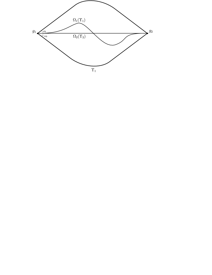
Figure 9.1: Domain $G$ with the boundary $\partial G=\bar{\Upsilon}_{1}\cup\bar{\Upsilon}_{2}$.

To each of the points $g_{1},g_{2}$, there corresponds the same model problem in the plane angle:

$$\Delta U =f_{0}(y)\quad(y\in K),$$ (9.3)

$$U|_{\gamma_{j}}+b_{j}U(\mathcal{G}_{j}y)|_{\gamma_{j}} =f_{j}(y)\quad(y\in\gamma_{j};\ j=1,2).$$ (9.4)

Here $K=\{y\in{\mathbb{R}}^{2}:r>0,\ |\omega|<\omega_{0}\}$, $\gamma_{j}=\{y\in{\mathbb{R}}^{2}:r>0,\ \omega=(-1)^{j}\omega_{0}\}$, and

$$\mathcal{G}_{j}=\begin{pmatrix}\cos\omega_{0}&(-1)^{j}\sin\omega_{0}\\ (-1)^{j+1}\sin\omega_{0}&\cos\omega_{0}\end{pmatrix}$$

is the operator of rotation by the angle $(-1)^{j+1}\omega_{0}$ around the origin, $j=1,2$.

The eigenvalues problem corresponding to problem (9.3), (9.4) has the following form:

$$\frac{d^{2}\varphi(\omega)}{d\omega^{2}}-\lambda^{2}\varphi(\omega)=0\quad(|\omega|<\omega_{0}),$$ (9.5)

$$\varphi(-\omega_{0})+b_{1}\varphi(0)=0,\quad\varphi(\omega_{0})+b_{2}\varphi(0)=0.$$ (9.6)

Let us find the eigenvalues of problem (9.5), (9.6).

I. First, we consider the case where $\lambda\neq 0$. Substituting the general solution $\varphi(\omega)=c_{1}e^{\lambda\omega}+c_{2}e^{-\lambda\omega}$ for Eq. (9.5) into nonlocal condition (9.6), we get the following system of equations:

$$\begin{pmatrix}e^{-\lambda\omega_{0}}+b_{1}&e^{\lambda\omega_{0}}+b_{1}\\ e^{\lambda\omega_{0}}+b_{2}&e^{-\lambda\omega_{0}}+b_{2}\end{pmatrix}\begin{pmatrix}c_{1}\\ c_{2}\end{pmatrix}=\begin{pmatrix}0\\ 0\end{pmatrix}.$$ (9.7)

Equating the determinant of system (9.7) with zero, we get

$$(e^{-\lambda\omega_{0}}-e^{\lambda\omega_{0}})(e^{\lambda\omega_{0}}+e^{-\lambda\omega_{0}}+b_{1}+b_{2})=0.$$

1. From the equation $e^{-\lambda\omega_{0}}-e^{\lambda\omega_{0}}=0$, we obtain

$$\lambda=\frac{\pi k}{\omega_{0}}i,\quad k\in{\mathbb{Z}}\setminus\{0\}.$$ (9.8)

2. Let us consider the equation $e^{\lambda\omega_{0}}+e^{-\lambda\omega_{0}}+b_{1}+b_{2}=0$. If $b_{1}+b_{2}=0$, then

$$\lambda=\frac{\pi/2+\pi k}{\omega_{0}}i,\quad k\in{\mathbb{Z}}.$$ (9.9)

If $b_{1}+b_{2}\neq 0$, then

$$\lambda^{\pm}=\left\{\begin{aligned} &\frac{\ln\left(-\frac{b_{1}+b_{2}}{2}\pm\frac{\sqrt{(b_{1}+b_{2})^{2}-4}}{2}\right)}{\omega_{0}}+\frac{2\pi n}{\omega_{0}}i\ &\mbox{for }&b_{1}+b_{2}<-2,\\ &\frac{\pm{\rm arctg\,}\frac{\sqrt{4-(b_{1}+b_{2})^{2}}}{b_{1}+b_{2}}+2\pi n}{\omega_{0}}i\ &\mbox{for }&-2<b_{1}+b_{2}<0,\\ &\frac{\pm{\rm arctg\,}\frac{\sqrt{4-(b_{1}+b_{2})^{2}}}{b_{1}+b_{2}}+(2n+1)\pi}{\omega_{0}}i\ &\mbox{for }&0<b_{1}+b_{2}<2,\\ &\frac{\ln\left(\frac{b_{1}+b_{2}}{2}\pm\frac{\sqrt{(b_{1}+b_{2})^{2}-4}}{2}\right)}{\omega_{0}}+\frac{(2n+1)\pi}{\omega_{0}}i\ &\mbox{for }&b_{1}+b_{2}>2,\end{aligned}\right.$$ (9.10)

$n\in{\mathbb{Z}}$. For $|b_{1}+b_{2}|=2$, we get the eigenvalues from the series (9.8).

II. Similarly, one can consider the case where $\lambda=0$ and verify that $\lambda=0$ is an eigenvalue of problem (9.5), (9.6) if and only if $b_{1}+b_{2}=-2$.

Let us study the particular case where $\omega_{0}=\pi/2$, which implies that $\partial G\in C^{\infty}$.

I. Let $\lambda\neq 0$.

1. From (9.8), we get the following pure imaginary eigenvalues with integer imaginary parts:

$$\lambda_{2k}=2ki,\quad k\in{\mathbb{Z}}\setminus\{0\}.$$ (9.11)

2. If $b_{1}+b_{2}=0$, we get from (9.9) the following pure imaginary eigenvalues with integer imaginary parts:

$$\lambda_{2k+1}=(2k+1)i,\quad k\in{\mathbb{Z}}.$$ (9.12)

If $b_{1}+b_{2}\neq 0$, we get from (9.10) the following eigenvalues:

$$\lambda_{n}^{\pm}=\left\{\begin{aligned} &\frac{2\ln\left(-\frac{b_{1}+b_{2}}{2}\pm\frac{\sqrt{(b_{1}+b_{2})^{2}-4}}{2}\right)}{\pi}+4ni\ &\mbox{for }&b_{1}+b_{2}<-2,\\ &\frac{\pm 2{\rm arctg\,}\frac{\sqrt{4-(b_{1}+b_{2})^{2}}}{b_{1}+b_{2}}}{\pi}i+4ni\ &\mbox{for }&-2<b_{1}+b_{2}<0,\\ &\frac{\pm 2{\rm arctg\,}\frac{\sqrt{4-(b_{1}+b_{2})^{2}}}{b_{1}+b_{2}}}{\pi}i+(4n+2)i\ &\mbox{for }&0<b_{1}+b_{2}<2,\\ &\frac{2\ln\left(\frac{b_{1}+b_{2}}{2}\pm\frac{\sqrt{(b_{1}+b_{2})^{2}-4}}{2}\right)}{\pi}+(4n+2)i\ &\mbox{for }&b_{1}+b_{2}>2,\end{aligned}\right.$$ (9.13)

$n\in{\mathbb{Z}}$. If $|b_{1}+b_{2}|=2$, we get the eigenvalues from the series (9.11).

II. The number $\lambda_{0}=0$ is an eigenvalue of problem (9.5), (9.6) if and only if $b_{1}+b_{2}=-2$.

Let us consider the operator $\mathbf{L}:W^{l+2}(G)\to\mathcal{W}^{l}(G,\Upsilon)$ corresponding to problem (9.1), (9.2) with $\omega_{0}=\pi/2$. From (9.11)–(9.13) and Theorem 4.1, we derive the following result.

Theorem 9.1.

Suppose that $\omega_{0}=\pi/2$. Let $l$ be even; then the operator $\mathbf{L}:W^{l+2}(G)\to\mathcal{W}^{l}(G,\Upsilon)$ is Fredholm if and only if $b_{1}+b_{2}\neq 0$.

Let $l$ be odd; then the operator $\mathbf{L}:W^{l+2}(G)\to\mathcal{W}^{l}(G,\Upsilon)$ is not Fredholm for any $b_{1},b_{2}\in\mathbb{R}$.

Notice that if $l$ is even and $b_{1}=b_{2}=0$, then the operator $\mathbf{L}$ corresponding to the “local” boundary-value problem is not Fredholm (its image is not closed). However, if we add nonlocal terms with arbitrary small coefficient $b_{1},b_{2}$ (such that $b_{1}+b_{2}\neq 0$) in the boundary-value conditions, the problem becomes Fredholm.

9.1.2 Problem with homogeneous nonlocal conditions

Let us study problem (9.1), (9.2) with homogeneous nonlocal conditions in the case where $\omega_{0}=\pi/2$. We denote

$$W_{B}^{l+2}(G)=\left\{u\in W^{l+2}(G):u|_{\Upsilon_{i}}+b_{i}u\bigl{(}\Omega_{i}(y)\bigr{)}\big{|}_{\Upsilon_{i}}=0,\ i=1,2\right\}$$

and introduce the corresponding operator $\mathbf{L}_{B}:W_{B}^{l+2}(G)\to W^{l}(G)$ given by

$$\mathbf{L}_{B}u=\Delta u,\quad u\in W_{B}^{l+2}(G).$$

The Fredholm solvability of the operator $\mathbf{L}_{B}$ is influenced only by the eigenvalues of problem (9.5), (9.6), lying on the line ${\rm Im\,}\lambda=-(l+1)$, $l\geq 0$. Thus, we have to consider only the eigenvalues (9.11), (9.12) for $k\leq-1$ and (9.13) for $|b_{1}+b_{2}|>2$, $n\leq-1$. Clearly, the eigenvalues (9.13) for $|b_{1}+b_{2}|>2$ are improper since they are not pure imaginary. Therefore, let us begin with the question when the eigenvalues (9.11) and (9.12) are proper.

1. Consider the numbers $\lambda_{2k}=2ki$, $k=-1,-2,\dots$, which are eigenvalues of problem (9.5), (9.6) for any $b_{1},b_{2}$. Let us show that $\lambda_{2k}$ is a proper eigenvalue if and only if $b_{1}+b_{2}\neq 2(-1)^{k+1}$.

To the eigenvalue $\lambda_{2k}$, there corresponds the eigenvector $\varphi_{2k}^{(0)}(\omega)=e^{i2k\omega}-e^{-i2k\omega}=2i\sin(2k\omega)$ (and, for $b_{1}=b_{2}=(-1)^{k+1}$, there is the second eigenvector $\psi_{2k}^{(0)}(\omega)=e^{i2k\omega}+e^{-i2k\omega}=2\cos(2k\omega)$). If an associate vector $\varphi_{2k}^{(1)}$ exists, then it satisfies the equation

$$\frac{d^{2}\varphi_{2k}^{(1)}(\omega)}{d\omega^{2}}+4k^{2}\varphi_{2k}^{(1)}(\omega)=4ik\varphi_{2k}^{(0)}(\omega)\quad(|\omega|<\pi/2)$$ (9.14)

and nonlocal conditions (9.6). Substituting the general solution

$$\varphi_{2k}^{(1)}(\omega)=c_{1}e^{i2k\omega}+c_{2}e^{-i2k\omega}+\omega(e^{i2k\omega}+e^{-i2k\omega})$$

for Eq. (9.14) into nonlocal conditions (9.6), we get the following system of equations for $c_{1},c_{2}$:

$$\begin{pmatrix}(-1)^{k}+b_{1}&(-1)^{k}+b_{1}\\ (-1)^{k}+b_{2}&(-1)^{k}+b_{2}\end{pmatrix}\begin{pmatrix}c_{1}\\ c_{2}\end{pmatrix}=\begin{pmatrix}\pi(-1)^{k}\\ -\pi(-1)^{k}\end{pmatrix}.$$

Clearly, this system is incompatible if and only if $b_{1}+b_{2}\neq 2(-1)^{k+1}$. Combining this with the fact that $r^{-2k}\varphi_{2k}^{(0)}(\omega)$ is a polynomial with respect to $y_{1},y_{2}$ for $k=-1,-2,\dots$, we see that $\lambda_{2k}$ is a proper eigenvalue if and only if $b_{1}+b_{2}\neq 2(-1)^{k+1}$.

2. Consider the numbers $\lambda_{2k+1}=(2k+1)i,\ k=-1,-2,\dots$, which are eigenvalues of problem (9.5), (9.6) if and only if $b_{1}+b_{2}=0$. Let us prove that, for $b_{1}+b_{2}=0$, the eigenvalues $\lambda_{2k+1}$ are proper ones.

To the eigenvalue $\lambda_{2k+1}$, there corresponds the unique eigenvector $\varphi_{2k+1}^{(0)}(\omega)=e^{i(2k+1)\omega}+e^{-i(2k+1)\omega}=2i\sin((2k+1)\omega)$. If an associate eigenvector $\varphi_{2k+1}^{(1)}$ exists, then it satisfies the equation

$$\frac{d^{2}\varphi_{2k+1}^{(1)}(\omega)}{d\omega^{2}}+(2k+1)^{2}\varphi_{2k+1}^{(1)}(\omega)=2i(2k+1)\varphi_{2k+1}^{(0)}(\omega)\quad(|\omega|<\pi/2)$$ (9.15)

and nonlocal conditions (9.6). Substituting the general solution

$$\varphi_{2k+1}^{(1)}(\omega)=c_{1}e^{i(2k+1)\omega}+c_{2}e^{-i(2k+1)\omega}+\omega(e^{i(2k+1)\omega}-e^{-i(2k+1)\omega})$$

for Eq. (9.15) into nonlocal conditions (9.6), we get the following system of equations for $c_{1},c_{2}$:

$$\begin{pmatrix}-i(-1)^{k}+b_{1}&i(-1)^{k}+b_{1}\\ i(-1)^{k}+b_{2}&-i(-1)^{k}+b_{2}\end{pmatrix}\begin{pmatrix}c_{1}\\ c_{2}\end{pmatrix}=\begin{pmatrix}-i\pi(-1)^{k}\\ -i\pi(-1)^{k}\end{pmatrix}.$$

Clearly, this system is incompatible for $b_{1}+b_{2}=0$. Combining this with the fact that $r^{-(2k+1)}\varphi_{2k+1}^{(0)}(\omega)$ is a polynomial with respect to $y_{1},y_{2}$ for $k=-1,-2,\dots$, we see that, for $b_{1}+b_{2}=0$, the eigenvalues $\lambda_{2k+1}$ are proper.

Remark 9.1.

While checking whether an eigenvalue is proper, we sought only for a first associate vector. Obviously, we can continue this procedure and find the whole Jordan chain (see, e.g., Example 2.1 in [29]); however, we do not do this here, since the existence of a first associate vector already implies that the corresponding eigenvalue is improper.

I. Consider the operator $\mathbf{L}_{B}:W_{B}^{2}(G)\to L_{2}(G)$. The line ${\rm Im\,}\lambda=-1$ contains either no eigenvalues of problem (9.5), (9.6) (if $b_{1}+b_{2}\neq 0$) or only the proper eigenvalue $\lambda_{-1}=-i$ (if $b_{1}+b_{2}=0$). Applying either Theorem 8.1 (if $b_{1}+b_{2}\neq 0$) or Theorem 8.2 (if $b_{1}+b_{2}=0$), we see that the operator $\mathbf{L}_{B}:W_{B}^{2}(G)\to L_{2}(G)$ is Fredholm for all $b_{1},b_{2}$.

II. Consider the operator $\mathbf{L}_{B}:W_{B}^{3}(G)\to W^{1}(G)$.

(a) Let $b_{1}+b_{2}>2$. Then the line ${\rm Im\,}\lambda=-2$ contains the proper eigenvalue $\lambda_{-2}=-2i$ and the two improper eigenvalues $\lambda_{-2}^{\pm}=\dfrac{2\ln\left(\frac{b_{1}+b_{2}}{2}\pm\frac{\sqrt{(b_{1}+b_{2})^{2}-4}}{2}\right)}{\pi}-2i$. Therefore, by Theorem 8.1, the operator $\mathbf{L}_{B}:W_{B}^{3}(G)\to W^{1}(G)$ is not Fredholm.

(b) Let $b_{1}+b_{2}=2$. Then the line ${\rm Im\,}\lambda=-2$ contains only the improper eigenvalue $\lambda_{-2}=-2i$. Therefore, by Theorem 8.1, the operator $\mathbf{L}_{B}:W_{B}^{3}(G)\to W^{1}(G)$ is not Fredholm.

(c) Let $b_{1}+b_{2}<2$. Then the line ${\rm Im\,}\lambda=-2$ contains only the proper eigenvalue $\lambda_{-2}=-2i$. We have to check Condition 8.2. Differentiating the expression $U(y)+b_{j}U(\mathcal{G}_{j}y)$ with respect to $y_{2}$ twice and replacing the values of the corresponding function at the point $\mathcal{G}_{j}y$ by the values at $y$, we see that system (2.12) has the following form:

$$\hat{\mathcal{B}}_{1}(D_{y})U=\frac{\partial^{2}U}{\partial y_{2}^{2}}+b_{1}\frac{\partial^{2}U}{\partial y_{1}^{2}},\quad\hat{\mathcal{B}}_{2}(D_{y})U=\frac{\partial^{2}U}{\partial y_{2}^{2}}+b_{2}\frac{\partial^{2}U}{\partial y_{1}^{2}}$$

1. Let $b_{1}\neq b_{2}$. Then the operators $\hat{\mathcal{B}}_{1}(D_{y})U$ and $\hat{\mathcal{B}}_{2}(D_{y})U$ are linearly independent and, therefore, both included in system (3.4). Clearly, the operator $\Delta U$ is not included in this system, since the system

   $${\mathcal{B}}_{1}(D_{y})U,\quad\hat{\mathcal{B}}_{2}(D_{y})U,\quad\Delta U$$

   is linearly dependent. Hence, Condition 8.2 fails, and Theorem 8.2 implies that the operator $\mathbf{L}_{B}:W_{B}^{3}(G)\to W^{1}(G)$ is not Fredholm.

2. Let $b_{1}=b_{2}$ (and, therefore, $b_{1}=b_{2}<1$). Then the operators $\hat{\mathcal{B}}_{1}(D_{y})U$ and $\hat{\mathcal{B}}_{2}(D_{y})U$ coincide. Since $b_{1}<1$, the system

   $$\hat{\mathcal{B}}_{1}(D_{y})U,\quad\Delta U$$

   is linearly independent and constitutes system (3.4). Hence, Condition 8.2 holds, and Theorem 8.2 implies that the operator $\mathbf{L}_{B}:W_{B}^{3}(G)\to W^{1}(G)$ is Fredholm.

Thus, we proved that the operator $\mathbf{L}_{B}:W_{B}^{3}(G)\to W^{1}(G)$ is Fredholm if and only if $b_{1}=b_{2}<1$.

III. Consider the operator $\mathbf{L}_{B}:W_{B}^{l+2}(G)\to W^{l}(G)$ with even $l\geq 2$.

(a) Let $b_{1}+b_{2}\neq 0$. Then the line ${\rm Im\,}\lambda=-(l+1)$ contains no eigenvalues of problem (9.5), (9.6). Therefore, by Theorem 8.2, the operator $\mathbf{L}_{B}:W_{B}^{l+2}(G)\to W^{l}(G)$ is Fredholm.

(b) Let $b_{1}+b_{2}=0$. Then the line ${\rm Im\,}\lambda=-(l+1)$ contains only the proper eigenvalue $\lambda_{-(l+1)}=-(l+1)i$. Unlike the case where $l=0$, now we have to check Condition 8.2. Differentiating the expression $U(y)+b_{j}U(\mathcal{G}_{j}y)$ with respect to $y_{2}$  $l+1$ times and replacing the values of the corresponding function at the point $\mathcal{G}_{j}y$ by the values at $y$, we see that system (2.12) has the form

$$\hat{\mathcal{B}}_{1}(D_{y})U=\frac{\partial^{l+1}U}{\partial y_{2}^{l+1}}-b_{1}\frac{\partial^{l+1}U}{\partial y_{1}^{l+1}},\quad\hat{\mathcal{B}}_{2}(D_{y})U=\frac{\partial^{l+1}U}{\partial y_{2}^{l+1}}+b_{2}\frac{\partial^{l+1}U}{\partial y_{1}^{l+1}}.$$

Since $b_{2}=-b_{1}$, only the operator $\hat{\mathcal{B}}_{1}(D_{y})U$ is included in system (3.4).

Let us show that the system consisting of the operator $\hat{\mathcal{B}}_{1}(D_{y})U$ and

$$\frac{\partial^{l-1}}{\partial y_{1}^{\xi_{1}}\partial y_{2}^{\xi_{2}}}\Delta U\equiv\frac{\partial^{l+1}U}{\partial y_{1}^{\xi_{1}+2}\partial y_{2}^{\xi_{2}}}+\frac{\partial^{l+1}U}{\partial y_{1}^{\xi_{1}}\partial y_{2}^{\xi_{2}+2}}\quad(\xi_{1}+\xi_{2}=l-1)$$

is linearly independent. To this end, we associate with each derivative $\dfrac{\partial^{l+1}U}{\partial y_{1}^{s}\partial y_{2}^{l+1-s}}$, $s=0,\dots,l+1$, the vector

$$(0,\dots,0,1,0,\dots,0)$$

of length $l+2$ such that its $(s+1)$st component is equal to one while all the remaining components are equal to zero. Then the operator $\hat{\mathcal{B}}_{1}(D_{y})U$ is associated with the vector

$$(1,0,\dots,0,-b_{1})$$ (9.16)

and the operators $\dfrac{\partial^{l-1}}{\partial y_{1}^{\xi_{1}}\partial y_{2}^{\xi_{2}}}\Delta$, $\xi_{1}=0,\dots,l-1$, are associated with the vectors

$$(0,\dots,1,0,1,\dots,0)$$ (9.17)

such that their $(\xi_{1}+1)$st and $(\xi_{1}+3)$rd components are equal to one while all the remaining components are equal to zero. Thus, we have to show that the rank of the $\big{(}(l+1)\times(l+2)\big{)}$ order matrix

$$A=\begin{pmatrix}1&0&0&0&\dots&0&0&-b_{1}\\ 1&0&1&0&\dots&0&0&0\\ 0&1&0&1&\dots&0&0&0\\ \vdots&\vdots&\vdots&\vdots&\ddots&\vdots&\vdots&\vdots\\ 0&0&0&0&\dots&1&0&0\\ 0&0&0&0&\dots&0&1&0\\ 0&0&0&0&\dots&1&0&1\\ \end{pmatrix}$$

consisting of the rows (9.16), (9.17) is equal to $l+1$. We denote by $A^{\prime}$ the matrix obtained from the matrix $A$ by deleting the last column. Decomposing the determinant of $A^{\prime}$ by the first row, we see that $\det A^{\prime}=\det A_{l}$, where

$$A_{l}=\begin{pmatrix}0&1&0&\dots&0&0&0\\ 1&0&1&\dots&0&0&0\\ 0&1&0&\dots&0&0&0\\ \vdots&\vdots&\vdots&\ddots&\vdots&\vdots&\vdots\\ 0&0&0&\dots&0&1&0\\ 0&0&0&\dots&1&0&1\\ 0&0&0&\dots&0&1&0\end{pmatrix}$$

is a tridiagonal matrix of order $l\times l$. By induction, one can easily check that

$$\det A_{l}=\left\{\begin{aligned} 0\quad&\mbox{for}&l&=2n-1,\\ 1\quad&\mbox{for}&l&=4n,\\ -1\quad&\mbox{for}&l&=4n-2,\\ \end{aligned}\right.$$ (9.18)

$n\geq 1$. From (9.18), it follows that $|\det A^{\prime}|=|\det A_{l}|=1$. Therefore, the system

$$\hat{\mathcal{B}}_{1}(D_{y})U,\quad\frac{\partial^{l-1}}{\partial y_{1}^{\xi_{1}}\partial y_{2}^{\xi_{2}}}\Delta U\ (\xi_{1}+\xi_{2}=l-1)$$

is linearly independent, and Theorem 8.2 implies that the operator $\mathbf{L}_{B}:W_{B}^{l+2}(G)\to W^{l}(G)$ is Fredholm.

Thus we proved that the operator $\mathbf{L}_{B}:W_{B}^{l+2}(G)\to W^{l}(G)$ with even $l\geq 2$ is Fredholm for any $b_{1},b_{2}$.

IV. Finally, we consider the operator $\mathbf{L}_{B}:W_{B}^{l+2}(G)\to W^{l}(G)$ with odd $l\geq 3$. First, we assume that $l+1=4n$ for some $n\geq 1$.

(a) Let $b_{1}+b_{2}<-2$. Then the line ${\rm Im\,}\lambda=-(l+1)=-4n$ contains the proper eigenvalue $\lambda_{-4n}=-4ni$ and the two improper eigenvalues $\lambda_{-4n}^{\pm}=\dfrac{2\ln\left(\frac{b_{1}+b_{2}}{2}\pm\frac{\sqrt{(b_{1}+b_{2})^{2}-4}}{2}\right)}{\pi}-4ni$. Therefore, by Theorem 8.1, the operator $\mathbf{L}_{B}:W_{B}^{l+2}(G)\to W^{l}(G)$ is not Fredholm.

(b) Let $b_{1}+b_{2}=-2$. Then the line ${\rm Im\,}\lambda=-(l+1)=-4n$ contains only the improper eigenvalue $\lambda_{-4n}=-4ni$. Therefore, by Theorem 8.1, the operator $\mathbf{L}_{B}:W_{B}^{l+2}(G)\to W^{l}(G)$ is not Fredholm.

(c) Let $b_{1}+b_{2}>-2$. Then the line ${\rm Im\,}\lambda=-(l+1)=-4n$ contains only the proper eigenvalue $\lambda_{-2}=-4ni$. We have to check Condition 8.2. Differentiating the expression $U(y)+b_{j}U(\mathcal{G}_{j}y)$ with respect to $y_{2}$  $l+1$ times and replacing the values of the corresponding function at the point $\mathcal{G}_{j}y$ by the values at $y$, we see that system (2.12) has the form

$$\hat{\mathcal{B}}_{1}(D_{y})U=\frac{\partial^{l+1}U}{\partial y_{2}^{l+1}}+b_{1}\frac{\partial^{l+1}U}{\partial y_{1}^{l+1}},\quad\hat{\mathcal{B}}_{2}(D_{y})U=\frac{\partial^{l+1}U}{\partial y_{2}^{l+1}}+b_{2}\frac{\partial^{l+1}U}{\partial y_{1}^{l+1}}.$$

1. Let $b_{1}\neq b_{2}$. Then the operators $\hat{\mathcal{B}}_{1}(D_{y})U$ and $\hat{\mathcal{B}}_{2}(D_{y})U$ are linearly independent and, therefore, both included in system (3.4). Let us show that the system

   $$\hat{\mathcal{B}}_{1}(D_{y})U,\quad\hat{\mathcal{B}}_{2}(D_{y})U,\quad\frac{\partial^{l-1}}{\partial y_{1}^{\xi_{1}}\partial y_{2}^{\xi_{2}}}\Delta U\ (\xi_{1}+\xi_{2}=l-1)$$

   is linearly dependent. (Notice that, unlike the case where $l=1$, this system now contains all the $l+1$ order derivatives of $U$.) Since $\hat{\mathcal{B}}_{1}(D_{y})U$ and $\hat{\mathcal{B}}_{2}(D_{y})U$ are linearly independent, it suffices to show that the system

   $$\frac{\partial^{l+1}U}{\partial y_{2}^{l+1}},\quad\frac{\partial^{l+1}U}{\partial y_{1}^{l+1}},\quad\frac{\partial^{l-1}}{\partial y_{1}^{\xi_{1}}\partial y_{2}^{\xi_{2}}}\Delta U\ (\xi_{1}+\xi_{2}=l-1)$$

   is linearly dependent. We consider the corresponding matrix

   $$A=\begin{pmatrix}1&0&0&0&\dots&0&0&0\\ 0&0&0&0&\dots&0&0&1\\ 1&0&1&0&\dots&0&0&0\\ 0&1&0&1&\dots&0&0&0\\ \vdots&\vdots&\vdots&\vdots&\ddots&\vdots&\vdots&\vdots\\ 0&0&0&0&\dots&1&0&0\\ 0&0&0&0&\dots&0&1&0\\ 0&0&0&0&\dots&1&0&1\\ \end{pmatrix}$$

   of order $(l+2)\times(l+2)$. Decomposing the determinant of $A$ by the first row and then decomposing the determinant of the matrix which we obtained by the first row again, we see that $\det A=\det A_{l}$. Since $l$ is odd, it follows from (9.18) that $\det A=0$. Therefore, Condition 8.2 fails, and Theorem 8.2, implies that the operator $\mathbf{L}_{B}:W_{B}^{l+2}(G)\to W^{l}(G)$ is not Fredholm.

2. Let $b_{1}=b_{2}$ (and, therefore, $b_{1}=b_{2}>-1$). Then system (3.4) contains only the operator $\hat{\mathcal{B}}_{1}(D_{y})U$. Let us show that the system

   $$\hat{\mathcal{B}}_{1}(D_{y})U,\quad\frac{\partial^{l-1}}{\partial y_{1}^{\xi_{1}}\partial y_{2}^{\xi_{2}}}\Delta U\ (\xi_{1}+\xi_{2}=l-1)$$

   is linearly independent. We consider the corresponding matrix

   $$A=\begin{pmatrix}1&0&0&0&\dots&0&0&b_{1}\\ 1&0&1&0&\dots&0&0&0\\ 0&1&0&1&\dots&0&0&0\\ \vdots&\vdots&\vdots&\vdots&\ddots&\vdots&\vdots&\vdots\\ 0&0&0&0&\dots&1&0&0\\ 0&0&0&0&\dots&0&1&0\\ 0&0&0&0&\dots&1&0&1\\ \end{pmatrix}$$

   of order $(l+1)\times(l+2)$. Deleting the second column from $A$, decomposing the determinant of the matrix which we obtained by the first row, and using relation (9.18), we get

   $$\begin{vmatrix}1&0&0&\dots&0&0&b_{1}\\ 1&1&0&\dots&0&0&0\\ 0&0&1&\dots&0&0&0\\ \vdots&\vdots&\vdots&\ddots&\vdots&\vdots&\vdots\\ 0&0&0&\dots&1&0&0\\ 0&0&0&\dots&0&1&0\\ 0&0&0&\dots&1&0&1\end{vmatrix}=1-b_{1}\begin{vmatrix}1&1&0&\dots&0&0&0\\ 0&0&1&\dots&0&0&0\\ 0&1&0&\dots&0&0&0\\ \vdots&\vdots&\vdots&\ddots&\vdots&\vdots&\vdots\\ 0&0&0&\dots&0&1&0\\ 0&0&0&\dots&1&0&1\\ 0&0&0&\dots&0&1&0\end{vmatrix}=1-b_{1}\det A_{l-1}=1+b_{1}\neq 0$$

   since $b_{1}>-1$. Therefore, Condition 8.2 holds, and Theorem 8.2 implies that the operator $\mathbf{L}_{B}:W_{B}^{l+2}(G)\to W^{l}(G)$ is Fredholm.

Thus, we proved that the operator $\mathbf{L}_{B}:W_{B}^{l+2}(G)\to W^{l}(G)$ with $l+1=4n$, $n\geq 1$, is Fredholm if and only if $b_{1}=b_{2}>-1$.

Analogously, by using (9.18) and Theorem 8.2, one can show that the operator $\mathbf{L}_{B}:W_{B}^{l+2}(G)\to W^{l}(G)$ with $l+1=4n+2$, $n\geq 1$, is Fredholm if and only if $b_{1}=b_{2}<1$.

The following theorem summarize the results obtained.

Theorem 9.2.

Let $l$ be even; then the operator $\mathbf{L}_{B}:W_{B}^{l+2}(G)\to W^{l}(G)$ is Fredholm for any $b_{1},b_{2}\in\mathbb{R}$.

Let $l$ be odd and $l=4n+1,\ n=0,1,2,\dots$; then the operator $\mathbf{L}_{B}:W_{B}^{l+2}(G)\to W^{l}(G)$ is Fredholm if and only if $b_{1}=b_{2}<1$.

Let $l$ be odd and $l=4n+3,\ n=0,1,2,\dots$; then the operator $\mathbf{L}_{B}:W_{B}^{l+2}(G)\to W^{l}(G)$ is Fredholm if and only if $b_{1}=b_{2}>-1$.

Notice that, for $\omega_{0}=\pi/2$ and $b_{1}=b_{2}=0$, we have the “local” Dirichlet problem in a smooth domain with homogeneous boundary-value conditions. In this case, as is well known, the operator $\mathbf{L}_{B}:W_{B}^{l+2}(G)\to W^{l}(G)$ corresponding to problem (9.1), (9.2) with homogeneous boundary-value conditions is not only Fredholm for any $l\geq 0$ but also invertible.

9.2 Example 2

9.2.1 Problem with nonhomogeneous nonlocal conditions

Let $G\subset{\mathbb{R}}^{2}$ be a domain such that its boundary $\partial G\in C^{\infty}$ coincides, outside the disks $B_{1/8}((i4/3,j4/3))$ $(i,j=0,1)$, with the boundary of the square $(0,4/3)\times(0,4/3)$. We denote $\Upsilon_{1}=\{y\in\partial G:y_{1}<1/3,\ y_{2}<1/3\}$, $\Upsilon_{2}=\{y\in\partial G:y_{1}>1,\ y_{2}>1\}$, $\Upsilon_{3}=\partial G\setminus(\bar{\Upsilon}_{1}\cup\bar{\Upsilon}_{2})$. Thus, we have $\mathcal{K}=\{g_{1},\dots,g_{4}\}$, where $g_{1}=(1/3,0),\ g_{2}=(0,1/3),\ g_{3}=(4/3,1),\ g_{4}=(1,4/3)$ (see Fig. 9.2).

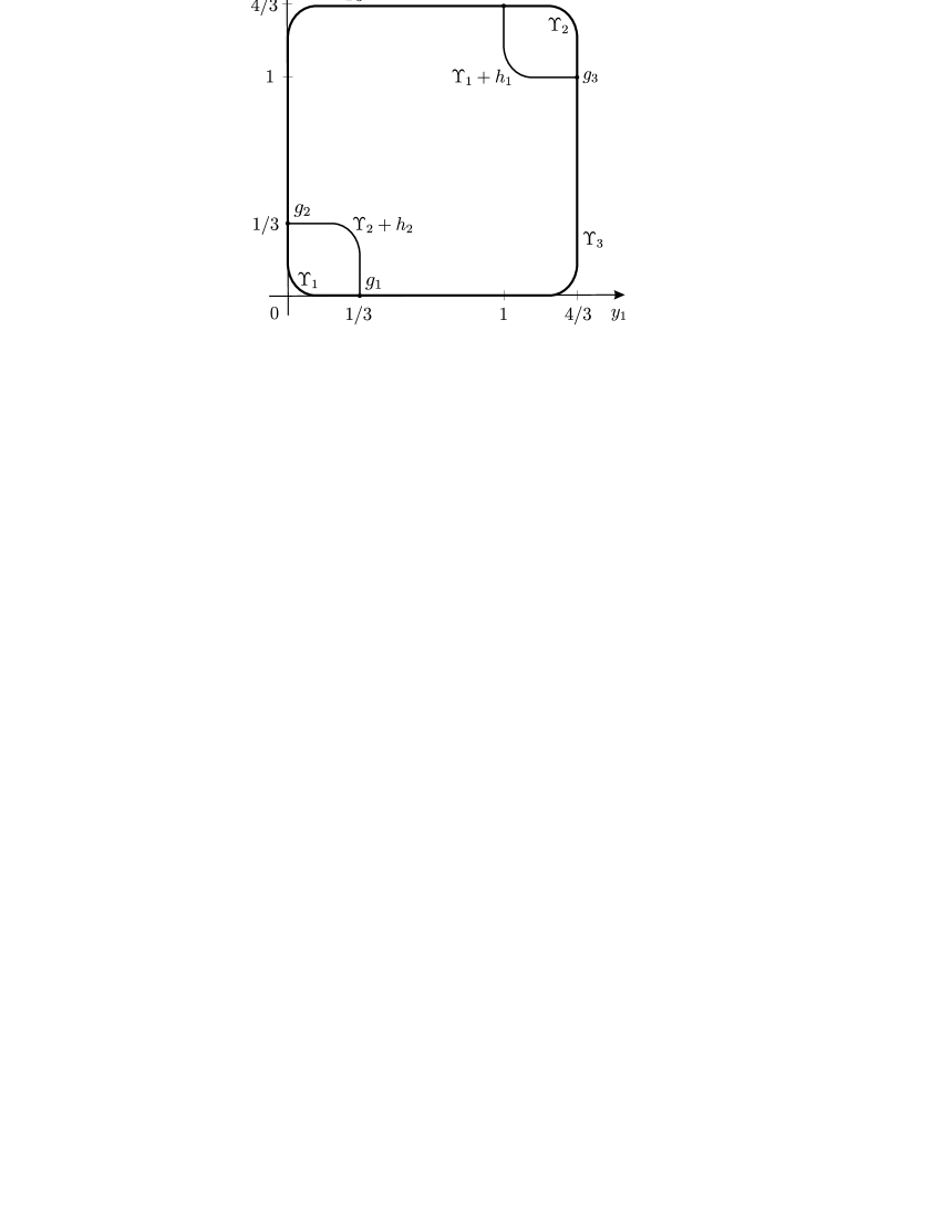
Figure 9.2: Domain $G$ with smooth boundary $\partial G=\bar{\Upsilon}_{1}\cup\bar{\Upsilon}_{2}\cup\bar{\Upsilon}_{3}$.

We consider the following nonlocal elliptic problem in the domain $G$:

$$\Delta u=f_{0}(y)\quad(y\in G),$$ (9.19)

$$u(y)|_{\Upsilon_{i}}+b_{i}u(y+h_{i})|_{\Upsilon_{i}} =f_{i}(y)\quad(y\in\Upsilon_{i};\ i=1,2),$$ (9.20)

$$u(y)|_{\Upsilon_{3}} =f_{3}(y)\quad(y\in\Upsilon_{3}),$$

where $h_{1}=(1,1)$, $h_{2}=(-1,-1)$, and $b_{1},b_{2}\in{\mathbb{R}}$. Clearly, $\mathcal{K}={\rm Orb}_{1}\cup{\rm Orb}_{2}$, where the orbit ${\rm Orb}_{1}$ consists of the points $g_{1}$ and $g_{3}=g_{1}+h_{1}$ and the orbit ${\rm Orb}_{2}$ consists of the points $g_{2}$ and $g_{4}=g_{2}+h_{2}$.

According to Remark 7.2, Condition 7.2 holds. Clearly, Condition 8.1 also holds.

First, we assume that $b_{1}^{2}+b_{2}^{2}\neq 0$ (for definiteness, we suppose that $b_{1}\neq 0$).

To each of the orbits ${\rm Orb}_{1},\ {\rm Orb}_{2}$, there corresponds the same model problem in the plane angles:

$$\Delta U_{j}=f_{j}(y)\quad(y\in K),$$ (9.21)

$$\begin{matrix}U_{1}|_{\gamma_{1}}=f_{11}(y)\ (y\in\gamma_{1}),\quad U_{1}|_{\gamma_{2}}+b_{1}U_{2}(\mathcal{G}y)|_{\gamma_{2}}=f_{12}(y)\ (y\in\gamma_{2}),\\ U_{2}|_{\gamma_{1}}=f_{21}(y)\ (y\in\gamma_{1}),\quad U_{2}|_{\gamma_{2}}+b_{2}U_{1}(\mathcal{G}y)|_{\gamma_{2}}=f_{22}(y)\ (y\in\gamma_{2}).\end{matrix}$$ (9.22)

Here $K=\{y\in{\mathbb{R}}^{2}:r>0,\ |\omega|<\pi/2\}$, $\gamma_{j}=\{y\in{\mathbb{R}}^{2}:r>0,\ \omega=(-1)^{j}\pi/2\}$, and $\mathcal{G}=\begin{pmatrix}0&1\\ -1&0\end{pmatrix}$ is the operator of rotation by the angle $-\pi/2$.

The eigenvalues problem corresponding to problem (9.21), (9.22) has the following form:

$$\frac{d^{2}\varphi_{j}(\omega)}{d\omega^{2}}-\lambda^{2}\varphi_{j}(\omega)=0\quad(|\omega|<\pi/2;\ j=1,2),$$ (9.23)

$$\begin{matrix}\varphi_{1}(-\pi/2)=0,\quad\varphi_{1}(\pi/2)+b_{1}\varphi_{2}(0)=0,\\ \varphi_{2}(-\pi/2)=0,\quad\varphi_{2}(\pi/2)+b_{2}\varphi_{1}(0)=0.\end{matrix}$$ (9.24)

One can find the eigenvalues of problem (9.23), (9.24) by straightforward computations (see [19]). They are

$$\lambda_{2k} =2ki,\quad k\in{\mathbb{Z}}\setminus\{0\}\quad(\text{for all }b_{1},b_{2},\ b_{1}^{2}+b_{2}^{2}\neq 0),$$ (9.25)

$$\lambda_{2k+1} =(2k+1)i,\quad k\in{\mathbb{Z}}\quad(\mbox{for }b_{2}=0,\ b_{1}\neq 0),$$ (9.26)

and

$$\lambda_{n}^{\pm}=\left\{\begin{aligned} &\frac{2}{\pi}\ln\left|\frac{\sqrt{-b_{1}b_{2}}}{2}\pm\frac{\sqrt{4-b_{1}b_{2}}}{2}\right|+(2n+1)i\ &\mbox{for }&b_{1}b_{2}<0,\\ &\left(\pm\frac{2}{\pi}{\rm arctg\,}\sqrt{4(b_{1}b_{2})^{-1}-1}+2n\right)i\ &\mbox{for }&0<b_{1}b_{2}<4,\\ &\frac{2}{\pi}\ln\left(\frac{\sqrt{b_{1}b_{2}}}{2}\pm\frac{\sqrt{b_{1}b_{2}-4}}{2}\right)+2ni&\mbox{for }&b_{1}b_{2}\geq 4,\end{aligned}\right.$$ (9.27)

$n\in{\mathbb{Z}}$. If $b_{1}b_{2}=4$, then there is one more eigenvalue $\lambda_{0}=0$.

Remark 9.2.

If $b_{2}=0$, we can consider the other statement of nonlocal problem different from (9.19), (9.20), namely:

$$\Delta u=f(y)\quad(y\in G),$$ (9.28)

$$u(y)|_{\Upsilon_{1}}+b_{1}u(y+h_{1})|_{\Upsilon_{1}} =f_{1}(y)\quad(y\in\Upsilon_{1}),$$ (9.29)

$$u(y)|_{\bar{\Upsilon}_{2}\cup\Upsilon_{3}} =f_{2}(y)\quad(y\in\bar{\Upsilon}_{2}\cup\Upsilon_{3}).$$

In this case, we have $\mathcal{K}=\{g_{1},g_{2}\}$ (notice that Condition 7.2 now fails). Solutions to problem (9.28), (9.29) may have singularities only near the points $g_{1},g_{2}$, while solutions to problem (9.19), (9.20) may have those near $g_{1},\dots,g_{4}$.

To each of the points $g_{1},g_{2}$, there corresponds the same model “local” problem:

$$\Delta U_{1}=f_{1}(y)\quad(y\in K),$$ (9.30)

$$U_{1}|_{\gamma_{1}}=f_{1}(y)\ (y\in\gamma_{1}),\quad U_{1}|_{\gamma_{2}}=f_{2}(y)\ (y\in\gamma_{2}).$$ (9.31)

The eigenvalues problem for problem (9.30), (9.31) has the following form:

$$\frac{d^{2}\varphi_{1}(\omega)}{d\omega^{2}}-\lambda^{2}\varphi_{1}(\omega)=0\quad(|\omega|<\pi/2),$$ (9.32)

$$\varphi_{1}(-\pi/2)=\varphi_{1}(\pi/2)=0.$$ (9.33)

The eigenvalues of problem (9.32), (9.33) are as follows:

$$\lambda_{k}=ki,\quad k\in{\mathbb{Z}}\setminus\{0\}.$$ (9.34)

They coincide with the eigenvalues of problem (9.23), (9.24) for $b_{2}=0$. Therefore, according to Theorem 4.1, problem (9.28), (9.29) is Fredholm if and only if problem (9.19), (9.20) is Fredholm.

Let us consider the operator $\mathbf{L}:W^{l+2}(G)\to\mathcal{W}^{l}(G,\Upsilon)$ corresponding to problem (9.19), (9.20). From (9.25)–(9.27) and Theorem 4.1, we derive the following result.

Theorem 9.3.

Let $l$ be even; then the operator $\mathbf{L}:W^{l+2}(G)\to\mathcal{W}^{l}(G,\Upsilon)$ is Fredholm if and only if $b_{1}b_{2}>0$.

Let $l$ be odd; then the operator $\mathbf{L}:W^{l+2}(G)\to\mathcal{W}^{l}(G,\Upsilon)$ is not Fredholm for any $b_{1},b_{2}\in\mathbb{R}$.

Notice that Theorem 9.3 is proved under the assumption that $b_{1}^{2}+b_{2}^{2}\neq 0$; but the operator $\mathbf{L}:W^{l+2}(G)\to\mathcal{W}^{l}(G,\Upsilon)$ with $b_{1}=b_{2}=0$ corresponding to problem (9.19), (9.20) is not Fredholm either. This follows from the fact that, to each of the points $g_{1},\dots,g_{4}\in\mathcal{K}$, there corresponds model problem (9.32), (9.33) with the eigenvalues (9.34) lying on the lines $-(l+1)$, $l\geq 0$.

9.2.2 Problem with homogeneous nonlocal conditions

Let us study problem (9.19), (9.20) with homogeneous nonlocal conditions. We denote

$$W_{B}^{l+2}(G)=\left\{u\in W^{l+2}(G):u|_{\Upsilon_{i}}+b_{i}u(y+h_{i})|_{\Upsilon_{i}}=0,\ i=1,2;\ u|_{\Upsilon_{3}}=0\right\}$$

and introduce the corresponding operator $\mathbf{L}_{B}:W_{B}^{l+2}(G)\to W^{l}(G)$ given by

$$\mathbf{L}_{B}u=\Delta u,\quad u\in W_{B}^{l+2}(G).$$

First, we assume that $b_{1}^{2}+b_{2}^{2}\neq 0$ (for definiteness, we again suppose that $b_{1}\neq 0$).

Remark 9.3.

Problem (9.28), (9.29) with homogeneous nonlocal conditions is equivalent to problem (9.19), (9.20) with $b_{2}=0$. Therefore, there is no need to study problem (9.28), (9.29) independently.

The Fredholm property of the operator $\mathbf{L}_{B}$ is influenced only by the eigenvalues of problem (9.23), (9.24), lying on the line ${\rm Im\,}\lambda=-(l+1)$, $l\geq 0$. Thus, we have to consider only the eigenvalues $\lambda_{2k}$, $\lambda_{2k+1}$ (if $b_{2}=0$), and $\lambda_{n}^{\pm}$ (if $b_{1}b_{2}<0$ or $b_{1}b_{2}\geq 4$) for $k,n\leq-1$. Clearly, the eigenvalues $\lambda_{n}^{\pm}$ (if $b_{1}b_{2}<0$ of $b_{1}b_{2}\geq 4$) are improper, since they are not pure imaginary. Therefore, let us begin with the question when the eigenvalues $\lambda_{2k}$ and $\lambda_{2k+1}$ (if $b_{2}=0$) are proper.

1. Consider the numbers $\lambda_{2k}=2ki$, $k=-1,-2,\dots$, which are eigenvalues of problem (9.23), (9.24) for any $b_{1},b_{2}$. Let us show that $\lambda_{2k}$ is a proper eigenvalue.

To the eigenvalue $\lambda_{2k}$, there correspond the two linearly independent eigenvectors

$$\bigl{(}\varphi_{1,2k}^{(0)}(\omega),\ \varphi_{2,2k}^{(0)}(\omega)\bigr{)} =\bigl{(}e^{i2k\omega}-e^{-i2k\omega},\ 0\bigr{)}=\bigl{(}2i\sin(2k\omega),\ 0\bigr{)},$$

$$\bigl{(}\psi_{1,2k}^{(0)}(\omega),\ \psi_{2,2k}^{(0)}(\omega)\bigr{)} =\bigl{(}0,\ e^{i2k\omega}-e^{-i2k\omega}\bigr{)}=\bigl{(}0,\ 2i\sin(2k\omega)\bigr{)}.$$

If an associate vector $(\varphi_{1,2k}^{(1)},\ \varphi_{2,2k}^{(1)})$ corresponding to the first of the eigenvectors exists, then it satisfies the equations

$$\frac{d^{2}\varphi_{1,2k}^{(1)}(\omega)}{d\omega^{2}}+4k^{2}\varphi_{1,2k}^{(1)}(\omega) =4ik(e^{i2k\omega}-e^{-i2k\omega})\quad(|\omega|<\pi/2),$$ (9.35)

$$\frac{d^{2}\varphi_{2,2k}^{(1)}(\omega)}{d\omega^{2}}+4k^{2}\varphi_{2,2k}^{(1)}(\omega) =0\quad(|\omega|<\pi/2)$$

and nonlocal conditions (9.24). Substituting the general solution

$$\varphi_{1,2k}^{(1)}(\omega) =c_{1}e^{i2k\omega}+c_{2}e^{-i2k\omega}+\omega(e^{i2k\omega}+e^{-i2k\omega}),$$

$$\varphi_{2,2k}^{(1)}(\omega) =c_{3}e^{i2k\omega}+c_{4}e^{-i2k\omega}$$

for Eqs. (9.35) into nonlocal conditions (9.24), we get the following system of equations for $c_{1},\dots,c_{4}$:

$$\begin{pmatrix}(-1)^{k}&(-1)^{k}&0&0\\ (-1)^{k}&(-1)^{k}&b_{1}&b_{1}\\ 0&0&(-1)^{k}&(-1)^{k}\\ b_{2}&b_{2}&(-1)^{k}&(-1)^{k}\end{pmatrix}\begin{pmatrix}c_{1}\\ c_{2}\\ c_{3}\\ c_{4}\end{pmatrix}=\begin{pmatrix}\pi(-1)^{k}\\ -\pi(-1)^{k}\\ 0\\ 0\end{pmatrix}.$$

It is easy to see that this system is incompatible; therefore, the first eigenvector has no associate ones. Similarly, one can check that the second eigenvector also has no associate ones. Combining this with the fact that $r^{-2k}\varphi_{j,2k}^{(0)}(\omega)$ and $r^{-2k}\psi_{j,2k}^{(0)}(\omega)$ ($j=1,2$) are polynomials with respect to $y_{1},y_{2}$ for $k=-1,-2,\dots$, we see that $\lambda_{2k}$ is a proper eigenvalue.

2. Consider the numbers $\lambda_{2k+1}=(2k+1)i$, $k=-1,-2,\dots$, which are eigenvalues of problem (9.23), (9.24) with $b_{2}=0$ (we remind that $b_{1}\neq 0$). Let us show that $\lambda_{2k+1}$ is an improper eigenvalue.

To the eigenvalue $\lambda_{2k+1}$, there corresponds the only eigenvector

$$\bigl{(}\varphi_{1,2k+1}^{(0)}(\omega),\ \varphi_{2,2k+1}^{(0)}(\omega)\bigr{)}=(e^{i(2k+1)\omega}+e^{-i(2k+1)\omega},\ 0)=(2\cos((2k+1)\omega),\ 0).$$

If an associate eigenvector $(\varphi_{1,2k+1}^{(1)},\ \varphi_{2,2k+1}^{(1)})$ exists, then it satisfies the equations

$$\frac{d^{2}\varphi_{1,2k+1}^{(1)}(\omega)}{d\omega^{2}}+(2k+1)^{2}\varphi_{1,2k+1}^{(1)}(\omega) =2(2k+1)i(e^{i(2k+1)\omega}+e^{-i(2k+1)\omega})\quad(|\omega|<\pi/2),$$ (9.36)

$$\frac{d^{2}\varphi_{2,2k+1}^{(1)}(\omega)}{d\omega^{2}}+(2k+1)^{2}\varphi_{2,2k+1}^{(1)}(\omega) =0\quad(|\omega|<\pi/2)$$

and nonlocal conditions (9.24). Substituting the general solution

$$\varphi_{1,2k}^{(1)}(\omega) =c_{1}e^{i(2k+1)\omega}+c_{2}e^{-i(2k+1)\omega}+\omega(e^{i(2k+1)\omega}-e^{-i(2k+1)\omega}),$$

$$\varphi_{2,2k}^{(1)}(\omega) =c_{3}e^{i(2k+1)\omega}+c_{4}e^{-i(2k+1)\omega}$$

for Eqs. (9.36) into nonlocal conditions (9.24), we get the following system of equations for $c_{1},\dots,c_{4}$:

$$\begin{pmatrix}i(-1)^{k+1}&i(-1)^{k}&0&0\\ i(-1)^{k}&i(-1)^{k+1}&b_{1}&b_{1}\\ 0&0&i(-1)^{k+1}&i(-1)^{k}\\ 0&0&i(-1)^{k}&i(-1)^{k+1}\end{pmatrix}\begin{pmatrix}c_{1}\\ c_{2}\\ c_{3}\\ c_{4}\end{pmatrix}=\begin{pmatrix}\pi i(-1)^{k+1}\\ \pi i(-1)^{k+1}\\ 0\\ 0\end{pmatrix}.$$

It is easy to see that this system is compatible. Therefore, $\lambda_{2k+1}$ is an improper eigenvalue.

I. Consider the operator $\mathbf{L}_{B}:W_{B}^{2}(G)\to L_{2}(G)$. The line ${\rm Im\,}\lambda=-1$ contains either no eigenvalues of problem (9.23), (9.24) (if $b_{1}b_{2}>0$) or the improper eigenvalue $\lambda_{-1}$ (if $b_{2}=0$) or $\lambda_{-1}^{\pm}$ (if $b_{1}b_{2}<0$). Therefore, by Theorem 8.1, the operator $\mathbf{L}_{B}:W_{B}^{2}(G)\to L_{2}(G)$ is Fredholm if and only if $b_{1}b_{2}>0$.

II. Consider the operator $\mathbf{L}_{B}:W_{B}^{3}(G)\to W^{1}(G)$.

(a). Let $b_{1}b_{2}\geq 4$. Then the line ${\rm Im\,}\lambda=-2$ contains the proper eigenvalue $\lambda_{-2}$ and the two improper eigenvalues $\lambda_{-1}^{\pm}$. Therefore, by Theorem 8.1, the operator $\mathbf{L}_{B}:W_{B}^{3}(G)\to W^{1}(G)$ is not Fredholm.

(b) Let $b_{1}b_{2}<4$. Then the line ${\rm Im\,}\lambda=-2$ contains only the proper eigenvalue $\lambda_{-2}=-2i$. Let us show that Condition 8.2 fails.

Differentiating the expressions $U_{1}(y)+b_{1}U_{2}(\mathcal{G}y)$ and $U_{2}(y)+b_{2}U_{1}(\mathcal{G}y)$ with respect to $y_{2}$ twice and replacing the values of the corresponding functions at the point $\mathcal{G}y$ by the values at $y$, we see that system (2.12) has the following form:

$$\hat{\mathcal{B}}_{11}(D_{y})U =\frac{\partial^{2}U_{1}}{\partial y_{2}^{2}},\quad\hat{\mathcal{B}}_{12}(D_{y})U=\frac{\partial^{2}U_{1}}{\partial y_{2}^{2}}+b_{1}\frac{\partial^{2}U_{2}}{\partial y_{1}^{2}},$$

$$\hat{\mathcal{B}}_{21}(D_{y})U =\frac{\partial^{2}U_{2}}{\partial y_{2}^{2}},\quad\hat{\mathcal{B}}_{22}(D_{y})U=\frac{\partial^{2}U_{2}}{\partial y_{2}^{2}}+b_{2}\frac{\partial^{2}U_{1}}{\partial y_{1}^{2}}.$$

Since $b_{1}\neq 0$, the operators $\hat{\mathcal{B}}_{11}(D_{y})U$, $\hat{\mathcal{B}}_{12}(D_{y})U$, and $\hat{\mathcal{B}}_{21}(D_{y})U$ are linearly independent and, therefore, included in system (3.4). But the system consisting of these three operators and the operators $\Delta U_{1}$ and $\Delta U_{2}$ is linearly dependent. Therefore, Condition 8.2 fails, and Theorem 8.2 implies that the operator $\mathbf{L}_{B}:W_{B}^{3}(G)\to W^{1}(G)$ is not Fredholm.

Thus, we proved that the operator $\mathbf{L}_{B}:W_{B}^{3}(G)\to W^{1}(G)$ is not Fredholm for any $b_{1},b_{2}$ ($b_{1}^{2}+b_{2}^{2}\neq 0$).

III. Consider the operator $\mathbf{L}_{B}:W_{B}^{l+2}(G)\to W^{l}(G)$ with even $l\geq 2$. The line ${\rm Im\,}\lambda=-(l+1)$ contains either no eigenvalues of problem (9.23), (9.24) (if $b_{1}b_{2}>0$) or the improper eigenvalue $\lambda_{-(l+1)}$ (if $b_{2}=0$) of $\lambda_{-1-l/2}^{\pm}$ (if $b_{1}b_{2}<0$). Therefore, by Theorem 8.1, the operator $\mathbf{L}_{B}:W_{B}^{l+2}(G)\to W^{l}(G)$ with even $l\geq 2$ is Fredholm if and only if $b_{1}b_{2}>0$.

IV. Consider the operator $\mathbf{L}_{B}:W_{B}^{l+2}(G)\to W^{l}(G)$ with odd $l\geq 3$.

(a) Let $b_{1}b_{2}\geq 4$. Then the line ${\rm Im\,}\lambda=-(l+1)$ contains the proper eigenvalue $\lambda_{-(l+1)}$ and the two improper eigenvalues $\lambda_{-1/2-l/2}^{\pm}$. Therefore, by Theorem 8.1, the operator $\mathbf{L}_{B}:W_{B}^{l+2}(G)\to W^{l}(G)$ is not Fredholm.

(b) Let $b_{1}b_{2}<4$. Then the line ${\rm Im\,}\lambda=-(l+1)$ contains only the proper eigenvalue $\lambda_{-(l+1)}=-(l+1)i$. Let us show that Condition 8.2 fails. Differentiating the expressions $U_{1}(y)+b_{1}U_{2}(\mathcal{G}y)$ and $U_{2}(y)+b_{2}U_{1}(\mathcal{G}y)$ with respect to $y_{2}$  $l+1$ times and replacing the values of the corresponding functions at the point $\mathcal{G}y$ by the values at $y$, we see that system (2.12) has the following form:

$$\hat{\mathcal{B}}_{11}(D_{y})U =\frac{\partial^{l+1}U_{1}}{\partial y_{2}^{l+1}},\quad\hat{\mathcal{B}}_{12}(D_{y})U=\frac{\partial^{l+1}U_{1}}{\partial y_{2}^{l+1}}+b_{1}\frac{\partial^{l+1}U_{2}}{\partial y_{1}^{l+1}},$$

$$\hat{\mathcal{B}}_{21}(D_{y})U =\frac{\partial^{l+1}U_{2}}{\partial y_{2}^{l+1}},\quad\hat{\mathcal{B}}_{22}(D_{y})U=\frac{\partial^{l+1}U_{2}}{\partial y_{2}^{l+1}}+b_{2}\frac{\partial^{l+1}U_{1}}{\partial y_{1}^{l+1}}.$$

Since $b_{1}\neq 0$, the operators $\hat{\mathcal{B}}_{11}(D_{y})U$, $\hat{\mathcal{B}}_{12}(D_{y})U$, and $\hat{\mathcal{B}}_{21}(D_{y})U$ are linearly independent and, therefore, included in system (3.4). Let us show that the system of these three operators and

$$\frac{\partial^{l-1}}{\partial y_{1}^{\xi_{1}}\partial y_{2}^{\xi_{2}}}\Delta U_{1} \equiv\frac{\partial^{l+1}U_{1}}{\partial y_{1}^{\xi_{1}+2}\partial y_{2}^{\xi_{2}}}+\frac{\partial^{l+1}U_{1}}{\partial y_{1}^{\xi_{1}}\partial y_{2}^{\xi_{2}+2}}\quad(\xi_{1}+\xi_{2}=l-1),$$

$$\frac{\partial^{l-1}}{\partial y_{1}^{\xi_{1}}\partial y_{2}^{\xi_{2}}}\Delta U_{2} \equiv\frac{\partial^{l+1}U_{2}}{\partial y_{1}^{\xi_{1}+2}\partial y_{2}^{\xi_{2}}}+\frac{\partial^{l+1}U_{2}}{\partial y_{1}^{\xi_{1}}\partial y_{2}^{\xi_{2}+2}}\quad(\xi_{1}+\xi_{2}=l-1)$$

is linearly dependent. To this end, we associate with each derivative $\dfrac{\partial^{l+1}U_{1}}{\partial y_{1}^{s}\partial y_{2}^{l+1-s}}$, $s=0,\dots,l+1$, the vector

$$(0,\dots,0,1,0,\dots,0)$$

of length $2l+4$ such that its $(s+1)$st component is equal to one while all the remaining components are equal to zero. Further, we associate with each derivative $\dfrac{\partial^{l+1}U_{2}}{\partial y_{1}^{s}\partial y_{2}^{l+1-s}}$, $s=0,\dots,l+1$, the vector

$$(0,\dots,0,1,0,\dots,0)$$

of length $2l+4$ such that its $(l+2+s+1)$st component is equal to one while all the remaining components are equal to zero. Thus, it suffices to show that the rank of the $(2l+3)\times(2l+4)$ order matrix

$$A=\begin{pmatrix}1&0&0&\dots&0\rule{11.38109pt}{0.0pt}\vrule&0&0&0&\dots&0\\ 1&0&0&\dots&0\rule{11.38109pt}{0.0pt}\vrule&0&0&0&\dots&b_{1}\\ 0&0&0&\dots&0\rule{11.38109pt}{0.0pt}\vrule&1&0&0&\dots&0\\ \hline\cr 1&0&1&\dots&0\rule{11.38109pt}{0.0pt}\vrule&0&0&0&\dots&0\\ 0&1&0&\dots&0\rule{11.38109pt}{0.0pt}\vrule&0&0&0&\dots&0\\ \vdots&\vdots&\vdots&\ddots&\vdots\rule{14.22636pt}{0.0pt}\vrule&\vdots&\vdots&\vdots&\ddots&\vdots\\ 0&0&0&\dots&1\rule{11.38109pt}{0.0pt}\vrule&0&0&0&\dots&0\\ \hline\cr 0&0&0&\dots&0\rule{11.38109pt}{0.0pt}\vrule&1&0&1&\dots&0\\ 0&0&0&\dots&0\rule{11.38109pt}{0.0pt}\vrule&0&1&0&\dots&0\\ \vdots&\vdots&\vdots&\ddots&\vdots\rule{14.22636pt}{0.0pt}\vrule&\vdots&\vdots&\vdots&\ddots&\vdots\\ 0&0&0&\dots&0\rule{11.38109pt}{0.0pt}\vrule&0&0&0&\dots&1\end{pmatrix}$$

is less than $2l+3$. (In the matrix $A$, the first three rows correspond to the operators $\hat{\mathcal{B}}_{11}(D_{y})U$, $\hat{\mathcal{B}}_{12}(D_{y})U$, and $\hat{\mathcal{B}}_{21}(D_{y})U$ respectively, the next $l+2$ rows correspond to the operators $\dfrac{\partial^{l-1}}{\partial y_{1}^{\xi_{1}}\partial y_{2}^{\xi_{2}}}\Delta U_{1}$, and the last $l+2$ rows correspond to the operators $\dfrac{\partial^{l-1}}{\partial y_{1}^{\xi_{1}}\partial y_{2}^{\xi_{2}}}\Delta U_{2}$.)

If we delete the $1$st, $(l+3)$rd, or $(2l+4)$th columns from $A$, then the $1$st row, the $3$rd row, or the difference between the $1$st and $2$nd rows in the square matrix which we obtained is equal to zero. Let us denote by $\hat{A}$ the matrix which is obtained from $A$ by deleting any other column. Then, decomposing the determinant of $\hat{A}$ consecutively by the first three rows, we see that $|\det\hat{A}|=|b_{1}\det A^{\prime}|$, where $A^{\prime}$ is the $2l\times 2l$ order matrix that is obtained from the $2l\times(2l+1)$ order matrix

$$A^{\prime\prime}=\begin{pmatrix}0&1&\dots&0\rule{11.38109pt}{0.0pt}\vrule&0&0&\dots&0&0\\ 1&0&\dots&0\rule{11.38109pt}{0.0pt}\vrule&0&0&\dots&0&0\\ \vdots&\vdots&\ddots&\vdots\rule{14.22636pt}{0.0pt}\vrule&\vdots&\vdots&\ddots&\vdots&\vdots\\ 0&0&\dots&1\rule{11.38109pt}{0.0pt}\vrule&0&0&\dots&0&0\\ \hline\cr 0&0&\dots&0\rule{11.38109pt}{0.0pt}\vrule&0&1&\dots&0&0\\ 0&0&\dots&0\rule{11.38109pt}{0.0pt}\vrule&1&0&\dots&0&0\\ \vdots&\vdots&\ddots&\vdots\rule{14.22636pt}{0.0pt}\vrule&\vdots&\vdots&\ddots&\vdots&\vdots\\ 0&0&\dots&0\rule{11.38109pt}{0.0pt}\vrule&0&0&\dots&1&0\end{pmatrix}$$

by deleting the corresponding column. Notice that the last $l$ rows of $A^{\prime\prime}$ constitute the matrix $(0\ A_{l})$ and, by virtue of (9.18), are linearly dependent. Therefore, after deleting any column from $A^{\prime\prime}$, we again obtain a degenerate matrix. Hence, $\det\hat{A}=0$ and the rank of the matrix $A$ is less than $2l+3$. Thus, Condition 8.2 does fail, and Theorem 8.2 implies that the operator $\mathbf{L}_{B}:W_{B}^{l+2}(G)\to W^{l}(G)$ is not Fredholm.

So, we proved that the operator $\mathbf{L}_{B}:W_{B}^{l+2}(G)\to W^{l}(G)$ with odd $l\geq 3$ is not Fredholm for any $b_{1},b_{2}$.

We considered the case where $b_{1}^{2}+b_{2}^{2}\neq 0$. If $b_{1}=b_{2}=0$, one can similarly show that the corresponding operator $\mathbf{L}_{B}:W_{B}^{l+2}(G)\to W^{l}(G)$ is Fredholm for any $l\geq 0$. However, we omit the proof of this fact since, for $b_{1}=b_{2}=0$, we have the “local” Dirichlet problem in a smooth domain. As is well known, such a problem is not only Fredholm but uniquely solvable for any $l\geq 0$.

The following theorem summarize the results obtained.

Theorem 9.4.

Let $l$ be even; then the operator $\mathbf{L}_{B}:W_{B}^{l+2}(G)\to W^{l}(G)$ is Fredholm if and only if $b_{1}b_{2}>0$ or $b_{1}=b_{2}=0$.

Let $l$ be odd; then the operator $\mathbf{L}_{B}:W_{B}^{l+2}(G)\to W^{l}(G)$ is Fredholm if and only if $b_{1}=b_{2}=0$.

The author is grateful to A. L. Skubachevskii for attention to this work.

References

- [1] W. Feller, “Diffusion processes in one dimension,” Trans. Amer. Math. Soc., 77, 1–30 (1954).
- [2] A. A. Samarskii, “On some problems of theory of differential equations,” Differentsial’nye Uravneniya, 16, No. 11, 1925–1935 (1980); English transl.: Diff. Equ., 16 (1980).
- [3] G. G. Onanov, A. L. Skubachevskii, “Differential equations with displaced arguments in stationary problems in the mechanics of a deformed body,” Prikladnaya Mekhanika, 15, 39–47 (1979); English transl.: Soviet Applied Mech., 15 (1979).
- [4] A. Sommerfeld, “Ein Beitrag zur hydrodinamischen Erklärung der turbulenten Flussigkeitsbewegungen,” Proc. Intern. Congr. Math. (Rome, 1908), Reale Accad. Lincei. Roma. 3, 116–124 (1909).
- [5] J. D. Tamarkin, Some General Problems of the Theory of Ordinary Linear Differential Equations and Expansion of an Arbitrary Function in Series of Fundamental Functions, Petrograd, 1917. Abridged English transl.: Math. Z., 27, 1–54 (1928).
- [6] M. Picone, “Equazione integrale traducente il più generale problema lineare per le equazioni differenziali lineari ordinarie di qualsivoglia ordine,” Academia nazionale dei Lincei. Atti dei convegni., 15, 942–948 (1932).
- [7] T. Carleman, “Sur la théorie des equations integrales et ses applications,” Verhandlungen des Internat. Math. Kongr. Zürich., 1, 132–151 (1932).
- [8] A. V. Bitsadze, A. A. Samarskii, “On some simple generalizations of linear elliptic boundary value problems,” Dokl. Akad. Nauk SSSR., 185, 739–740 (1969); English transl.: Soviet Math. Dokl., 10 (1969).
- [9] S. D. Eidelman, N. V. Zhitarashu, “Nonlocal boundary value problems for elliptic equations,” Mat. Issled., 6, No. 2 (20), 63–73 (1971) [in Russian].
- [10] Ya. A. Roitberg, Z. G. Sheftel’, “Nonlocal problems for elliptic equations and systems,” Sib. Mat. Zh., 13 (1972), 165–181; English transl.: Siberian Math. J., 13 (1972).
- [11] K. Yu. Kishkis, “The index of a Bitsadze–Samarskii Problem for harmonic functions,” Differentsial’nye Uravneniya., 24, No. 1, 105–110 (1988); English transl.: Diff. Equ., 24 (1988).
- [12] A. K. Gushchin, V. P. Mikhailov, “On solvability of nonlocal problems for elliptic equations of second order,” Mat. sb., 185, 121–160 (1994); English transl.: Math. Sb., 185 (1994).
- [13] A. L. Skubachevskii, “Nonlocal elliptic problems with a parameter,” Mat. Sb., 121 (163), 201–210 (1983); English transl.: Math. USSR Sb., 49 (1984).
- [14] A. L. Skubachevskii, “Elliptic problems with nonlocal conditions near the boundary,” Mat. Sb., 129 (171), 279–302 (1986); English transl.: Math. USSR Sb., 57 (1987).
- [15] A. L. Skubachevskii, “Model nonlocal problems for elliptic equations in dihedral angles,” Differentsial’nye Uravneniya, 26, 119–131 (1990); English transl.: Differ. Equ., 26 (1990).
- [16] A. L. Skubachevskii, “Truncation-function method in the theory of nonlocal problems,” Differentsial’nye Uravneniya, 27, 128–139 (1991); English transl.: Diff. Equ., 27 (1991).
- [17] A. L. Skubachevskii, Elliptic Functional Differential Equations and Applications, Basel–Boston–Berlin, Birkhäuser, 1997.
- [18] O. A. Kovaleva, A. L. Skubachevskii, “Solvability of nonlocal elliptic problems in weighted spaces,” Mat. Zametki., 67, 882–898 (2000); English transl.: Math. Notes., 67 (2000).
- [19] A. L. Skubachevskii, “Regularity of solutions for some nonlocal elliptic problem,” Russ. J. Math. Phys., 8, 365–374 (2001).
- [20] P. L. Gurevich, “Nonlocal problems for elliptic equations in dihedral angles and the Green formula,” Mitteilungen aus dem Mathem. Seminar Giessen, Math. Inst. Univ. Giessen, Germany, 247, 1–74 (2001).
- [21] V. A. Kondrat’ev, “Boundary value problems for elliptic equations in domains with conical or angular points,” Trudy Moskov. Mat. Obshch., 16, 209–292 (1967); English transl.: Trans. Moscow Math. Soc., 16 (1967).
- [22] J. L. Lions, E Magenes, Non-Homogeneous Boundary Value Problems and Applications, Vol. , Springer–Verlag, New York–Heidelberg–Berlin, 1972.
- [23] I. C. Gohberg, E. I. Sigal, “An operator generalization of the logarithmic residue theorem and the theorem of Rouché,” Mat. Sb., 84 (126), 607–629 (1971); English transl.: Math. USSR Sb., 13 (1971).
- [24] F. Riesz, Sz.-Nagy, Leçons d’Analyse Fonctionnelle, Deuxième édition, Budapest, 1953.
- [25] E. M. Stein Singular Integrals and Differentiability Properties of Functions, Princeton Univ. Press, Princeton, 1970.
- [26] M. S. Agranovich, M. I. Vishik, “Elliptic problems with a parameter and parabolic problems of general type,” Uspekhi Mat. Nauk, 19, 53–161 (1964); English transl.: Russian Math. Surveys, 19 (1964).
- [27] L. R. Volevich “Solvavility of boundary-value problems for general elliptic systems,” Mat. sb., 68, No. 3, 373–416 (1965).
- [28] S. G. Krein Linear Equations in Banach Spaces, Nauka, Moscow, 1971 [in Russian]; English transl.: Birkhäuser, Boston, 1982.
- [29] P. L. Gurevich, “Asymptotics of solutions for nonlocal elliptic problems in plane angles,” Trudy seminara imeni I. G. Petrovskogo, 23, 2003; English transl. J. Math. Sci., New York.
- [30] V. G. Maz’ya, B. A. Plamenevskii, “-estimates of solutions of elliptic boundary value problems in domains with edges,” Trudy Moskov. Mat. Obshch., 37, 49–93 (1978). English transl.: Trans. Moscow Math. Soc., 37 (1980).