Directional Cell Discovery in
Millimeter Wave Cellular Networks

Abstract

The acute disparity between increasing bandwidth demand and available spectrum has brought millimeter wave (mmWave) bands to the forefront of candidate solutions for the next-generation cellular networks. Highly directional transmissions are essential for cellular communication in these frequencies to compensate for higher isotropic path loss. This reliance on directional beamforming, however, complicates initial cell search since mobiles and base stations must jointly search over a potentially large angular directional space to locate a suitable path to initiate communication. To address this problem, this paper proposes a directional cell discovery procedure where base stations periodically transmit synchronization signals, potentially in time-varying random directions, to scan the angular space. Detectors for these signals are derived based on a Generalized Likelihood Ratio Test (GLRT) under various signal and receiver assumptions. The detectors are then simulated under realistic design parameters and channels based on actual experimental measurements at 28 GHz in New York City. The study reveals two key findings: (i) digital beamforming can significantly outperform analog beamforming even when digital beamforming uses very low quantization to compensate for the additional power requirements; and (ii) omnidirectional transmissions of the synchronization signals from the base station generally outperforms random directional scanning.

I Introduction

Millimeter wave (mmWave) systems between 30 and 300 GHz have attracted considerable recent attention for next-generation cellular networks [1, 2, 3, 4, 5, 6]. The mmWave bands offer orders of magnitude more spectrum than current cellular allocations – up to 200 times by some estimates. However, a key challenge in mmWave cellular is the signal range. Due to Friis’ Law [7], the high frequencies of mmWave signals result in large isotropic path loss (the free-space path loss grows with the frequency squared). Fortunately, the small wavelengths of these signals also enable large number of antenna elements to be placed in the same physical antenna area, thereby providing high beamforming (BF) gains that can theoretically more than compensate for the increase in isotropic path loss [8, 9].

However, for cellular systems, the reliance on highly directional transmissions significantly complicates initial cell search. While current cellular systems such as 3GPP LTE [10] have considerable support for beamforming and multi-antenna technologies, the underlying design assumption is that initial network discovery can be conducted entirely with omnidirectional transmissions or transmissions in fixed antenna patterns. LTE base stations, for example, generally do not apply beamforming when transmitting the synchronization and broadcast signals. Adaptive beamforming and user-specific directional transmissions are generally used only after the physical-layer access has been established.

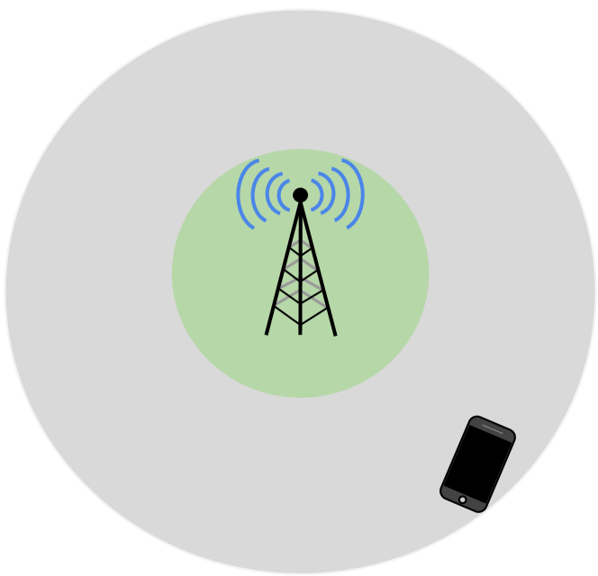
Figure 1: Due to highly directional transmissions, millimeter wave (mmWave) systems will exhibit a large disparity in the cell range in omnidirectional communication (green) vs. directional (gray). If cell search does not exploit this antenna gain, mobiles in the outer gray area may be capable of high data rates, but not able to locate the base station to establish the communication.

However, in the mmWave range, it may be essential to exploit antenna gain even during the cell search. Otherwise, the availability of high gain antennas would create a disparity between the range at which a cell can be detected (before the correct beamforming directions are known and the antenna gain is not available), and the range at which reasonable data rates can be achieved (after beamforming is used) – a point made in  [11] and [9, chapter 8] and also illustrated in Fig. 1. This disparity would in turn create a large area where a mobile may potentially be able to obtain a high data rate, but cannot realize this rate, since it cannot even detect the base station (BS).

To understand this directional cell search problem, this paper analyzes a standard cell search procedure where the base station periodically transmits synchronization signals and the mobiles scan for the presence of these signals to detect the base station, and learn the timing and direction of arrivals. This procedure is similar to the transmission of the Primary Synchronization Signal (PSS) in LTE [10], except here we consider three additional key design questions specific to directional transmissions in the mmWave range:

• How should mobiles jointly search for base stations and directions of arrival? The fundamental challenge for cell search in the mmWave range is the directional uncertainty. In addition to detecting the presence of base stations and their timing as required in conventional cell search, mmWave mobiles must also detect the spatial angles of transmissions on which the synchronization signals are being received.

• Should base stations transmit omnidirectionally or in randomly varying directions? We compare two different strategies for the base station transmitter: (i) the periodic synchronization signals are beamformed in randomly varying directions to scan the angular space, and (ii) the signals are transmitted in a fixed omnidirectional pattern. It is not obvious a priori which transmission strategy is preferable: randomly varying transmissions offers the possibility of occasional very strong signals at the mobile receiver, while using an omnidirectional transmission allows a constant power at the receiver. Note that, under uniform sampling of the angular directions, the average power must be the same in both cases due to Friis’ Law [7].

• What is the effect of analog vs. digital beamforming at the mobile? Due to the high bandwidths and large number of antenna elements in the mmWave range, it may not be possible from a power consumption perspective for the mobile receiver to obtain high rate digital samples from all antenna elements [12]. Most proposed designs perform beamforming in analog (either in RF or IF) prior to the A/D conversion [13, 14, 15, 16]. A key limitation for these architectures is that they permit the mobile to “look” in only one or a small number of directions at a time. To investigate the effect of this constraint we consider two detection scenarios: (i) analog beamforming where the mobile beamforms in a random angular direction in each PSS time slot; and (ii) digital beamforming where the mobile has access to digital samples from all the antenna elements. We will also consider hybrid beamforming [16, 17] – see Section IV-E.

The paper presents several contributions that may offer insight to the above-listed questions. First, to enable detection of the base stations in the presence of directional uncertainty, we derive generalized likelihood ratio test (GLRT) detectors [18] that treat the unknown spatial direction, delay and time-varying channel gains as unknown parameters. We show that for analog beamforming, the GLRT detection is equivalent to matched filter detection with non-coherent combining across multiple PSS time slots. For digital beamforming, the GLRT detector can be realized via a vector correlation across all the antennas followed by a maximal eigenvector that finds the optimal spatial direction. Both detectors are computationally easy to implement.

Second, to understand the relative performance of omnidirectional vs. random directions at the base station, we simulate the GLRT detectors under realistic system parameters and design requirements for both cases. A detailed discussion of how the synchronization channel parameters such as bandwidth, periodicity, and interval times should be selected is also given. The simulations indicate that, assuming GLRT detection, omnidirectional BS transmissions offer significant performance advantages in terms of detection time in comparison to the base station randomly varying its transmission angles. Of course, in either design, once a base station is detected, further procedures would be needed to more accurately determine and track the transmit and receive directions so that subsequent communication can be directional – we do not address this issue in this paper.

Finally, the simulations also indicate that using analog beamforming may result in a significant performance loss relative to digital beamforming. For example, in the simulations we present, where the mobile has a 4$\times$4 uniform 2D array, the loss is as much as 18 dB. Unfortunately, digital beamforming requires separate A/D converters for each antenna, which may be prohibitive from a power consumption standpoint in the bandwidths used in the mmWave range. However, the power consumption of the A/D can be dramatically reduced by using very low bit rates (say 2 to 3 bits per antenna) as proposed by [19, 20] and related methods in [21]. Using a standard white noise quantizer model [22], we show that, for the purpose of synchronization channel detection, the loss due to quantization noise with low bit rates is minimal. We thus conclude that low-bit rate fully digital front-ends may be a superior design choice in the mmWave range, at least for the purpose of cell search.

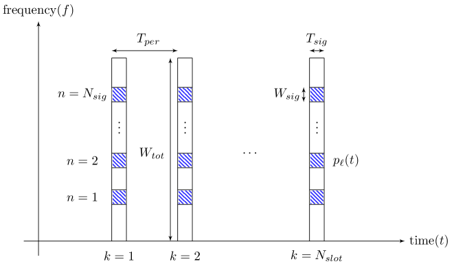
Figure 2: Proposed PSS periodic transmission.

A conference version of this paper has appeared in [23]. This paper includes all the derivations, discussion of the parameter selection, and more detailed, extensive simulations.

II Synchronization Signal Model

II-A Synchronization Channel in 3GPP LTE

We begin by briefly reviewing how synchronization channels are designed in LTE. A complete description can be found in [24]. In the current LTE standard, each base station cell (called the evolved NodeB or eNB) periodically broadcasts two signals: the Primary Synchronization Signal (PSS) and the Secondary Synchronization Signal (SSS). The mobiles (called the user equipment or UE) search for the cells by scanning various frequency bands for the presence of these signals. The mobiles first search for the PSS which provides a coarse estimate of the frame timing, frequency offset and receive power. To simplify the detection, only one of three PSS signals are transmitted. Once the PSS is detected, the UE can then search for the SSS. Since the frame timing and frequency offset of the eNB are already determined at this point, the SSS can belong to a larger set of 168 waveforms. The index of the detected PSS and SSS waveforms together convey the eNB cell identity. Since there are 3 PSS signals and 168 SSS signals, up to (168)(3)=504 cell identities can be communicated with the two signal indices. After the PSS and SSS are detected, the UE can proceed to decode the broadcast channels in which further information of the base station can be read.

This cell search procedure is performed both by UEs in idle mode, either seeking to establish an initial access to a base station or to find an eNB cell to “camp on” for paging, or UEs that are already connected to an eNB and need to look for other eNBs for potential handover targets. After detecting an eNB through the cell search, UEs in idle mode can initiate a random access procedure to the cell to establish a connection to the eNB, should a transition to active mode be necessary. UEs that are already connected to a serving eNB can report the signal strengths of the detected cell IDs to the network, which can then command the UE to perform a handover to that cell.

II-B Proposed mmWave Synchronization Channel Model

In this work, we focus on the PSS design for mmWave systems, since this is the channel that needs to be most significantly changed for mmWave. We consider a PSS transmission scheme shown in Fig. 2. Similar to the LTE PSS, we assume the signal is transmitted periodically once every $T_{per}$ seconds in a brief interval of length $T_{sig}$. We will call the short interval of length $T_{sig}$ the PSS time slot, and the period of length $T_{per}$ between two PSS slots, the PSS period. The selection of $T_{sig}$, $T_{per}$ and other parameters will be discussed below. As mentioned in the Introduction, while LTE base stations generally transmit the PSS omnidirectionally or in a fixed direction, here we consider two transmission scenarios: (i) the base station transmits the synchronization signal omnidirectionally (similar to current LTE), and (ii) the base station randomly transmits the signal in a different direction in each PSS time slot, thereby randomly scanning the angular space. Deterministic search patterns, as in 802.11ad [9], could also be performed although not considered here.

Also, to exploit the higher bandwidths available in the mmWave range, we assume that, in each PSS time slot, the PSS waveform is transmitted over $N_{sig}$ PSS sub-signals with each sub-signal being transmitted over a small bandwidth $W_{sig}$. The use of multiple sub-signals can provide frequency diversity, and narrowband signaling supports very low power receivers with high SNR capabilities. In current LTE systems, the PSS signal is transmitted over a relatively narrowband of approximately 930 kHz, which is slightly less than the minimum possible system bandwidth of 1.08 MHz [24]. Note that the PSS signal must fit in the minimum possible bandwidth. A mobile searching for the base station does not know the actual bandwidth during cell search, so all base stations transmit the PSS over the same bandwidth. For mmWave systems, it is expected that the minimum bandwidth will be much larger than current 4G systems, so that a reasonable number of narrowband sub-signals can be accommodated, even in the minimum bandwidth.

III PSS Detector

III-A Signal Model

To understand the detection of the synchronization signal, consider the transmission of a PSS signal from a BS with $N_{tx}$ antennas to a mobile with $N_{rx}$ receive antennas. Index all the PSS sub-signals across all PSS time slots by $\ell$. Then, we can write the complex baseband waveform for the PSS transmission from the BS as

$$\mathbf{x}(t)=\sum_{\ell=-\infty}^{\infty}\mathbf{w}^{tx}_{\ell}p_{\ell}(t),$$

where $\mathbf{x}(t)\in{\mathbb{C}}^{N_{tx}}$ is the vector of complex signals to the $N_{tx}$ antennas, $p_{\ell}(t)$ is the scalar PSS sub-signal waveform in the $\ell$-th time-frequency slot and $\mathbf{w}^{tx}_{\ell}$ is the TX beamforming vector applied to the $\ell$-th sub-signal. Note that in case of omnidirectional transmission, $\mathbf{w}^{tx}_{\ell}$ will be a constant with all energy on a single antenna. Since the sub-signals are transmitted periodically with $N_{sig}$ sub-signals per PSS time slot, we will index the sub-signals so that

$$\mbox{support}(p_{\ell})\subseteq I_{k}:=[kT_{per},kT_{per}+T_{sig}]$$ , (1)

$$\ell\in J_{k}:=\left\{(k-1)N_{sig}+1,\ldots,kN_{sig}\right\},\hskip 14.22636pt$$

where $I_{k}$ is the interval in time for the $k$-th PSS time slot, and $J_{k}$ is the set of indices $\ell$ such that the sub-signal $p_{\ell}(t)$ is transmitted in $I_{k}$.

For the purpose of the UE detector, our analysis is based on two key assumptions: First, we will assume that the channel is flat in the $T_{sig}\times W_{sig}$ time-frequency region around each PSS sub-signal (Section IV will discuss the selection of the parameters to ensure this). Thus, the channel can be described by a sequence of channel matrices $\mathbf{H}_{\ell}\in{\mathbb{C}}^{N_{rx}\times N_{tx}}$ in case of directional transmission, and $\mathbf{H}_{\ell}\in{\mathbb{C}}^{N_{rx}}$ when the signal is transmitted omnidirectionally, representing the complex channel gain between the BS and mobile around the $\ell$-th PSS sub-signal. Secondly, we will assume that the channel is rank one, which corresponds physically to a single path with no angular dispersion. In this case, the channel gain matrix can be written as

$$\mathbf{H}_{\ell}=g_{\ell}\mathbf{u}\mathbf{v}^{*},$$

where $g_{\ell}$ is the small-scale fading of the channel in the $\ell$-th sub-signal and $\mathbf{u}$ and $\mathbf{v}$ are the RX and TX spatial signatures, which are determined by the large scale path directions and antenna patterns at the RX and TX. With $\mathbf{x}^{*}$ or $\mathbf{A}^{*}$ we denote the conjugate transpose of any vector $\mathbf{x}$ or matrix $\mathbf{A}$. Note that we use the rank one assumption only for deriving the detector – our simulations in Section IV will consider practical mmWave channels such as [8, 17] with higher rank. We assume that $\mathbf{u}$ and $\mathbf{v}$ do not change over the detection period – hence there is no dependence on $\ell$. Of course, the real channel may not be exactly flat around the PSS sub-signals and will also have some non-zero angular spread. While our detector will assume a single path channel, our simulations presented in Section IV consider a more accurate multipath channel.

Under these channel assumptions, the receiver will see a complex signal of the form,

$$\mathbf{y}(t)=\sum_{\ell=-\infty}^{\infty}\alpha_{\ell}\mathbf{u}p_{\ell}(t-\tau)+\mathbf{d}(t),$$ (2)

where $\mathbf{y}(t)$ is the vector of RX signals across the $N_{rx}$ antennas, $\tau$ is the delay of the PSS signal, $\alpha_{\ell}$ is the effective channel gain

$$\alpha_{\ell}=g_{\ell}\mathbf{v}^{*}\mathbf{w}^{tx}_{\ell},$$ (3)

and $\mathbf{d}(t)$ is AWGN.

III-B GLRT Detection with Digital RX Beamforming

The objective of the mobile receiver is to determine, for each possible delay offset $\tau$, whether a PSS signal is present at that delay or not. Since the PSS is periodic with period $T_{per}$, the receiver needs only to test delay hypotheses in the interval $\tau\in[0,T_{per}]$.

We first consider this PSS detection problem in the case when the mobile can perform digital RX beamforming. In this case, the mobile receiver has access to digital samples from each of the individual components of the vector $\mathbf{y}(t)$ in (2). We assume the UE has access to full resolution values of the $\mathbf{y}(t)$. We will address the issue of quantization noise – critical for digital beamforming – in Section IV and Appendix D. We also assume that the detection is performed using $N_{slot}$ PSS time slots of data with indices $k=1,\ldots,N_{slot}$. For a given delay candidate $\tau$, let $\mathbf{Y}_{\tau}$ be the subset of the received signal $\mathbf{y}(t)$ for these time slots,

$$\mathbf{Y}_{\tau}=\left\{\mathbf{y}(t)~{}\mid~{}t\in I_{k}+\tau,~{}k=1,\ldots,N_{slot}\right\},$$ (4)

where $I_{k}$ is defined in (1) and is the interval for the $k$-th PSS time slot. Note that there are in total $L=N_{sig}N_{slot}$ sub-signals in this period - each sub-signal indexed with $\ell$.

We can now pose the detection of the PSS signal as a binary hypothesis problem: For each delay candidate $\tau$, a PSS signal is either present with that delay (the $H_{1}$ hypothesis) or is not present (the $H_{0}$ hypothesis). Following (2), we will assume a signal model for the two hypotheses of the form

$$H_{1}:~{}\mathbf{y}(t)=\sum_{\ell=-\infty}^{\infty}\alpha_{\ell}\mathbf{u}p_{\ell}(t-\tau)+\mathbf{d}(t),$$ (5a)

$$H_{0}:~{}\mathbf{y}(t)=\mathbf{d}(t),$$ (5b)

where $\mathbf{d}(t)$ is complex white Gaussian noise with some power spectral density matrix $\nu\mathbf{I}$. Let ${\bm{\theta}}$ be the vector of all the unknown parameters,

$${\bm{\theta}}=(\mathbf{u},\nu,\alpha_{1},\ldots,\alpha_{L}).$$

This vector contains the unknown RX spatial direction, $\mathbf{u}$, the noise power density, $\nu$, and the complex gains $\alpha_{\ell}$, $\ell=1,\ldots,L$. Due to the presence of these unknown parameters, we use a Generalized Likelihood Ratio Test (GLRT) [18] to decide between the two hypotheses:

$$\Lambda(\tau):=\log\frac{\max_{{\bm{\theta}}}p(\mathbf{Y}_{\tau}|H_{1},{\bm{\theta}})}{\max_{{\bm{\theta}}}p(\mathbf{Y}_{\tau}|H_{0},{\bm{\theta}})}\underset{H_{0}}{\overset{H_{1}}{\gtrless}}\;t^{\prime},$$ (6)

where $t^{\prime}$ is a threshold and $p(\mathbf{Y}_{\tau}|H_{i},{\bm{\theta}})$ is the probability density of the received signal data $\mathbf{Y}_{\tau}$ under the hypothesis $H_{0}$ or $H_{1}$ and parameters ${\bm{\theta}}$. The GLR $\Lambda(\tau)$ is the ratio of the likelihoods under the two hypotheses, maximized under the unknown parameters. Note that although $\mathbf{Y}_{\tau}$ is a continuous signal, we assume that each PSS sub-signal lies in a finite dimensional signal space. Hence, the density is well-defined. Also, one can in principle add other unknown parameters into the channel model such as frequency errors due to Doppler shift or initial local oscillator (LO) offsets. However, it is computationally simpler to avoid adding another parameter into the GLRT. Instead, as we discuss in Section IV, we will account for frequency offset errors by discretizing the frequency space and repeating the test over a number of frequency hypotheses.

It is shown in Appendix A that the GLRT (6) can be evaluated via a simple correlation. Specifically, let $\mathbf{v}_{\ell}(\tau)$ be the normalized matched-filter detector for the $\ell$-th subsignal,

$$\mathbf{v}_{\ell}(\tau)=\frac{1}{\|p_{\ell}\|}\int p^{*}_{\ell}(t)\mathbf{y}(t-\tau)dt,\quad\|p_{\ell}\|^{2}:=\int|p(t)|^{2}dt.$$ (7)

Also, let $E(\tau)$ be the total received energy in the $N_{slot}$ PSS time slots under the delay $\tau$,

$$E(\tau)=\sum_{k=1}^{N_{slot}}\int_{I_{k}}\|\mathbf{y}(t-\tau)\|^{2}dt,$$ (8)

where $I_{k}$ is the interval for the $k$-th time slot. Then, it is shown that, for any threshold level $t^{\prime}$, there exists a threshold level $t$ such that the GLRT in (6) is equivalent to a test of the form,

$$T(\tau)=\frac{\sigma_{max}^{2}(\mathbf{V}(\tau))}{E(\tau)}\underset{H_{0}}{\overset{H_{1}}{\gtrless}}\;t$$ (9)

where $t$ is a threshold level, $\mathbf{V}(\tau)\in{\mathbb{C}}^{N_{rx}\times L}$ is the matrix

$$\mathbf{V}(\tau):=\left[\mathbf{v}_{1}(\tau),\cdots\mathbf{v}_{L}(\tau)\right],$$ (10)

and $\sigma_{max}(\mathbf{V}(\tau))$ is the largest singular value of the matrix. The detector has a natural interpretation: First, we perform a matched filter correlator for each sub-signal $p_{\ell}(t)$ on each of the vectors $\mathbf{y}(t)$ yielding a vector correlation output $\mathbf{v}_{\ell}(\tau)$. We then compute the maximum singular vector for the matrix $\mathbf{V}(\tau)$ which finds the energy in the most likely spatial direction across all the $L$ sub-signals. Note that the GLRT is invariant to scaling of the received signal $\mathbf{y}(t)$ since the channel gain is treated as unknown.

It should also be noted that finding the maximum singular vector does add some complexity relative to PSS searching in LTE which only needs matched filtering. However, finding a maximum singular vector can be performed relatively easily, for example, via a power method [25]. Thus, we anticipate that the computation should be feasible, particularly as other parts of the baseband processing would need to scale for the higher data rates.

III-C GLRT for Analog Beamforming

We next consider the hypothesis testing problem in the case when the mobile receiver can only perform beamforming in analog (either at RF or IF). In this case, for each PSS time slot $k$, the RX must select a receive beamforming vector $\mathbf{w}^{rx}_{k}\in{\mathbb{C}}^{N_{rx}}$ and then only observes the samples in this direction. If we let $z(t)$ be the scalar output from applying the beamforming vector $\mathbf{w}^{rx}_{k}$ to the received vector $\mathbf{y}(t)$, the signal model for the two hypotheses in (5) is transformed to

$$H_{1}:~{}z(t)=\sum_{\ell=-\infty}^{\infty}\beta_{\ell}p_{\ell}(t-\tau)+d(t),$$ (11a)

$$H_{0}:~{}z(t)=d(t),$$ (11b)

where $\beta_{\ell}$ is the effective gain after TX and RX beamforming and $d(t)$ is complex white Gaussian noise with some PSD $\nu$. From (3), the beamforming gain will be given by

$$\beta_{\ell}:=g_{\ell}{\mathbf{w}^{rx}_{k}}^{*}\mathbf{u}\mathbf{v}^{*}\mathbf{w}^{tx}_{k},$$ (12)

for all sub-signals $\ell$ in the time slot $k$ (i.e. $\ell\in J_{k}$). Here, we have assumed that both the TX and RX must apply the same beamforming gains ($1$ in omni case) for all sub-signals in the same PSS time slot. This requirement is necessary since, under analog beamforming, both the TX and RX can use only one beam direction at a time. The unknown parameters in the analog case can be described by the vector

$${\bm{\theta}}=(\nu,\beta_{1},\ldots,\beta_{L}),$$

which contains the unknown variance $\nu$ and the channel gains $\beta_{1},\ldots,\beta_{L}$.

Analogous to (6), we use a GLRT of the form

$$\Lambda(\tau):=\log\frac{\max_{{\bm{\theta}}}p(Z_{\tau}|H_{1},{\bm{\theta}})}{\max_{{\bm{\theta}}}p(Z_{\tau}|H_{0},{\bm{\theta}})}\underset{H_{0}}{\overset{H_{1}}{\gtrless}}\;t^{\prime},$$ (13)

where $t^{\prime}$ is a threshold level and $Z_{\tau}$ is defined similarly to (4) for the beamformed signal $z(t)$.

Similar to the digital case, this GLRT can be evaluated via a correlation. Let $v_{\ell}(\tau)$ be the normalized correlation of $z(t)$ with the sub-signal $p_{\ell}(t)$,

$$v_{\ell}(\tau)=\frac{1}{\|p_{\ell}\|}\int p^{*}_{\ell}(t)z(t-\tau)dt,\quad\|p_{\ell}\|^{2}:=\int|p(t)|^{2}dt.$$ (14)

It is shown in Appendix B that GLRT (13) is equivalent to a test of the form

$$T(\tau)=\frac{\|\mathbf{v}(\tau)\|^{2}}{E(\tau)}\underset{H_{0}}{\overset{H_{1}}{\gtrless}}\;t,$$ (15)

where $t$ is a threshold level and $\mathbf{v}(\tau)\in{\mathbb{C}}^{L}$ is the vector

$$\mathbf{v}(\tau):=\left[v_{1}(\tau),\cdots,v_{L}(\tau)\right],$$ (16)

and $E(\tau)$ is the energy in the $N_{slot}$ time slots,

$$E(\tau)=\sum_{k=1}^{N_{slot}}\int_{I_{k}}\|z(t-\tau)\|^{2}dt.$$ (17)

Thus, in the analog beamforming case, the GLRT is simply performed with non-coherently adding the energy from the matched filter outputs for the $L$ sub-signals. An identical detector can also be used for hybrid beamforming where the outputs from multiple streams are treated as separate measurements – see Section IV-E.

IV Simulation

We assess the performance of the directional correlation detector for three cases: analog, digital, and quasi-analog or hybrid BF. We provide some explanation regarding the latter at the end of this section. Although we have derived our detectors based on a flat single path channel, we simulate the detectors’ performance both for a single path channel, as well as multipath pathloss channel model [8] derived from actual measurements in New York City [26, 27, 28, 3, 29]. The parameters for the channels (Table I) are based on realistic system design considerations. A detailed discussion of the selection of these parameters is given in Appendix C. Briefly, the PSS parameters $T_{sig}$ and $W_{sig}$ and $T_{per}$ were selected to ensure the channel is roughly flat within each $T_{sig}\times W_{sig}$ PSS sub-signal time-frequency region based on typical time and frequency coherence bandwidths observed in [26, 29]. The parameter $T_{sig}$ was also selected sufficiently short so that the Doppler shift across the sub-signal would not be significant with moderate mobile velocities (30 km/h). The value $T_{per}$ was then selected to keep a low (2%) total PSS overhead ($=T_{sig}/T_{per}$). This is slightly above the 1.5% overhead of PSS in LTE. We assume that during each PSS slot only the synchronization signal is transmitted and nothing else. The value $N_{sig}=4$ was found by trial-and-error to give the best performance in terms of frequency diversity versus energy loss from non-coherent combining. Under these parameters, we selected $N_{slot}=50$ slots to perform the search, which corresponds to a search time of $N_{slot}T_{per}=$ $250$ ms – a reasonable time frame for initial access.

For the antenna arrays, we considered 2D uniform linear arrays with $4\times 4$ elements at the mobile, and $8\times 8$ at the base station. When needed, random directions were selected by applying the beamforming for a randomly selected horizontal and elevation angle. Note that this selection only requires random phases applied to the antenna elements – not magnitude.

To compute the threshold level $t$ in (9) and (15), we first computed a false alarm probability target with the formula

$$P_{FA}=\frac{R_{FA}}{N_{PSS}N_{dly}N_{FO}},$$

where $R_{FA}$ is the maximum false alarm rate per search period over all signal, delay and frequency offset hypotheses and $N_{PSS}$, $N_{dly}$ and $N_{FO}$ are, respectively, the number of signal, delay and frequency offset hypotheses. Again, the details of the selection are given in Appendix C. The delay hypotheses $N_{dly}$ were calculated assuming sampling at twice the PSS bandwidth so that $N_{dly}=2W_{sig}T_{per}$. The number of frequency offsets $N_{FO}$ hypotheses was computed so that the frequency search could cover both an initial local oscillator (LO) error of $\pm 1$ part per million (ppm) as well as Doppler shift up to 30 km/h at 28 GHz. We selected $N_{PSS}=3$ for the number of signal hypotheses as used in current 3GPP LTE. We then used a large number of Monte Carlo trials to find the threshold to meet the false alarm rate. Since $P_{FA}$ was very small, we extrapolated the tail distribution of the statistic to estimate the correct threshold analytically, assuming $\log\Pr(T>t)$ is quadratic in $t$ for large $t$.

IV-A Detection Performance with Single Path Omnidirectional Transmissions

Figure 3: Misdetection Probability vs. data SNR: base station transmits PSS omnidirectionally (solid), and in random directions (dashed). In both cases, the performance of analog (blue) and digital (magenta) beamforming are compared at the receiver end. Also, a quantized version of digital beamforming (black) shows the small loss due to low bit rate (3 bits) resolution. Target SNR for $R_{tgt}=$ 10 Mbps (red).

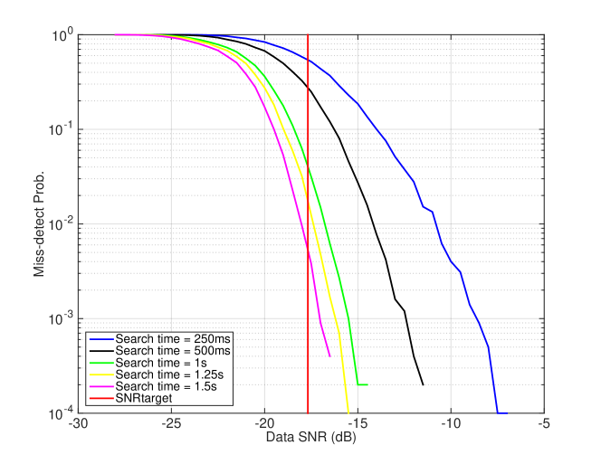
Figure 4: Misdetection Probability vs. data SNR: Omnidirectional transmission. The effect of increasing the search time while keeping the overhead fixed at $2\%$. Target SNR for $R_{tgt}=$ 10 Mbps (red)

First, we assessed the performance of the GLRT detectors in the case where the synchronization signal is transmitted omnidirectionally every $T_{per}$ seconds. The result is summarized in Fig. 3. The figure shows a large gap in SNR between digital and analog beamforming – more than 20 dB for $P_{MD}=0.01$. This gap is largely due to the fact that digital beamforming with the proposed eigenvector correlator can, in essence, determine the correct spatial direction over all the sub-signals, while analog beamforming can only “look” in one direction at a time.

The definition of SNR in Figures 3 through 6, requires some explanation. The SNR that determines the performance is what we will call the PSS SNR given by

$$\mbox{SNR}_{\rm PSS}=PT_{sig}/(N_{0}N_{sig}),$$ (18)

which is the SNR on a single PSS sub-signal for an omnidirectional received power $P$ and noise density $N_{0}$. However, the PSS SNR has no meaning outside the PSS signal. So, in Figures 3 through 6, we instead plot the misdetection rate against what we call the data SNR given by

$$\mbox{SNR}_{\rm data}=PG_{tx,max}G_{rx,max}/(N_{0}W_{tot}),$$ (19)

where $G_{tx,max}$ and $G_{rx,max}$ are the maximum possible beamforming gains and $W_{tot}$ is the total available bandwidth. The data SNR (19) is the theoretical SNR for a signal transmitted across the entire bandwidth $W_{tot}$ assuming optimal beamforming. The data SNR is related to the PSS SNR by

$$\mbox{SNR}_{\rm PSS}=\mbox{SNR}_{\rm data}\frac{T_{sig}W_{tot}}{N_{sig}G_{tx,max}G_{rx,max}}.$$ (20)

So, we simulate the PSS detection at the PSS SNR, but plot the result against the data SNR.

When plotted against the data SNR, it is easy to interpret the results of Fig. 3. For example, consider a typical edge rate minimum SNR requirement. Suppose that the UE should be able to connect whenever the SNR is sufficiently large to support some target rate, $R_{tgt}$. If the system was operating at the Shannon capacity with optimal beamforming, it would achieve this rate whenever the data SNR satisfies,

$$R_{tgt}=\beta W_{tot}\log_{2}\left(1+\mbox{SNR}_{\rm data}\right),$$

where $\beta$ is a bandwidth overhead fraction. Fig. 3 shows the target data SNR for $R_{tgt}$=10 Mbps, $W_{tot}=1$ GHz and $\beta=(0.5)(0.8)$ to account for half-duplexing TDD constraints and 20% control overhead [8]. From Fig. 3, we see that with digital beamforming, the system can reliably detect the signal at the SNR for the 10 Mbps rate target. But, with analog beamforming, the system needs a significantly larger SNR.

This edge rate requirement analysis also illustrates another issue. An edge rate target determines a minimum data SNR, which in turn determines the minimum PSS SNR. From (20), we see that for a given data SNR requirement, the PSS SNR decreases with the beamforming gain. In mmWave systems, this beamforming gain can be large. For example, in a single path channel, the beamforming gain is equal to the number of antennas. So, in our simulations, $G_{tx,max}=64$ and $G_{rx,max}=16$ for a combined total gain of 30 dBi. Gains of more than 20 dBi per side are not common in practical systems [6]. It is precisely this gain that makes the synchronization a challenge for mmWave systems: high antenna gains imply that the link can meet minimum rate requirements at very low SNRs once the link is established and directions are discovered. But, in order to use the links in the first place, the mobiles need to be able to detect the base stations at these low SNRs before the directions are known.

Note that the edge rate target would likely be determined by the point at which it is better to shift the mobiles from the 4G system. If a 100 Mbps edge rate were used, as suggested in [5, 6], the SNR target for which the mobile must detect the mmWave base station would be higher, making the detection requirement easier. However, using this target would imply less mobiles can be supported by 5G. Similarly, if the mmWave base station has a higher antenna gain, the PSS detection rate would be lower for the same data SNR. For example, if the base station had 256 antennas instead of 64 as assumed in this simulation, the data SNR would need to increase by 6 dB to maintain the same misdetection rate. Compensating for this SNR loss would necessitate longer detection times or more overhead.

Finally, given the results in Fig. 3, we wish to see if there is some way to improve analog beamforming’s performance. Fig. 4 shows that increasing the total search time by non-coherent combining over larger numbers of slots can lead to an improvement. However, the performance improvements show diminishing returns with increasing search time, and such long search times may induce intolerable delay overhead. Alternatively, we could keep the search time fixed and increase the overhead by transmitting the PSS signals more frequently. Either way, if we are to insist on an analog detector, sacrifices in searching time and possibly overhead may be necessary.

Parameter	Value
Total system bandwidth, $W_{tot}$	1 GHz
Number of sub-signals per PSS time slot, $N_{sig}$	$4$
Subsignal Duration, $T_{sig}$	$100$ $\mu$s
Subsignal Bandwidth, $T_{sig}$	1 MHz
Period between PSS transmissions, $T_{per}$	5 ms
PSS overhead	2%
Search period, $N_{slot}$	50 slots = 250 ms
Total false alarm rate per search period, $R_{FA}$	$0.01$
Number of PSS waveform hypotheses, $N_{PSS}$	$3$
Number of frequency offset hypotheses, $N_{FO}$	$23$
BS antenna	$8\times 8$ uniform linear array
UE antenna	$4\times 4$ uniform linear array
Carrier Frequency	28 GHz
PSS SNR, $PT_{sig}/N_{0}$	varied

TABLE I: Default simulation parameters unless otherwise stated.

IV-B Detection Performance with a Single Path Channel and Randomly Varying Transmission Angles

We next consider the case where the synchronization signal is transmitted in a random direction at every transmission instant. A deterministic search pattern, such as in 802.11ad [9] could also be used, but is not considered in this work. The simulation parameters remain the same as before and the results are also summarized in Fig. 3.

By switching to directional PSS transmission, the detector’s performance seems to degrade significantly: about $11$ dB in the analog case and $5$ dB with digital beamforming. In this case, as mentioned in Section III-C the analog detector sums up the match-filter’s output non-coherently for every given delay offset $\tau$. The reason for the degradation is that, when the base station transmits in random directions, the beams often “miss” the UE and the UE sees very little signal energy. In the omni case, on the other hand, although the signal loses about $18$ dB of potential TX beamforming gain, there is at least a constant (weak) power reception. The results are similar in other parameter settings, and we conclude that, for synchronization signals, randomly scanning angles at the transmitter is worse, in general, than using a constant omnidirectional transmission. It is worth noting that realistic omnidirectional mmWave antennas at the BS transmitter will likely use downtilt with significant gain on or below the horizon, just as is done in today’s cellular systems. In this case, some of the relative benefit of omnidirectional transmission over randomly varying directions will be reduced.

IV-C Detection Performance with Multipath Channels from New York City Data

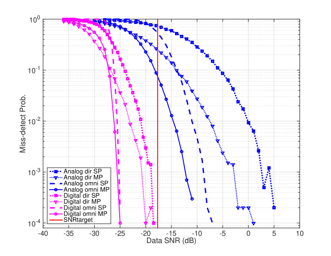
Figure 5: Misdetection Probability vs. data SNR: Single path channel versus multipath.

The above tests were based on a theoretical single path channel. Extensive measurements in New York City [26, 27, 28, 3, 29] revealed that in outdoor urban settings, the receiver can often see multiple macro-level scattering paths with significant angular spread. To validate the performance of our algorithm for these environments, we tested the algorithm under a realistic statistical spatial channel model [8] derived from the measurements in [26, 27, 28, 3, 29]. In this model, the channel is described by a random number of clusters, each cluster with a random vertical and horizontal angular spread – details are in [8]. Also, a more detailed statistical channel model is given in [30].

Fig. 5 illustrates the comparison between the single path vs. multipath channels. Interestingly, both analog and digital detectors perform better in multipath than for a single path, even though the detectors are designed based on a single-path assumption. In the digital case the performance gain of multipath over single path is small, while we observe a $4$ dB improvement in the analog case. This gain is due to the fact that the multipath channel creates more opportunities for the synchronization signal to be discovered when scanning signals at the receiver, particularly for analog BF where the receiver can search in only one direction at a time.

IV-D Quantization Effects

Of course, digital beamforming comes with a high power consumption cost since the A/D power consumption scales linearly with the number of antenna elements. However, since power consumption also scales exponentially with the number of bits, fully digital front ends may be feasible with very low bit rates per antenna as proposed in [19, 20, 21]. Using a linear white noise model for the quantizer [22], it is shown in Appendix D that the effective SNR after quantization can be approximated as

$$\gamma=\frac{(1-\alpha)\gamma_{0}}{1-\alpha+\alpha\gamma_{0}},$$

where $\gamma_{0}=P/(N_{0}W_{tot})$ is the SNR with no quantization error, $\gamma$ is the effective SNR with quantization error and $\alpha$ is the average relative error of the quantizer. Now, for a scalar uniform quantizer with only 3 bits, the relative error with optimal input level (assuming no errors in the AGC), is $\alpha\approx 0.035$. Using the value for $P/N_{0}$ at the target data rate, the gap between $\gamma_{0}$ and $\gamma$ is less than 0.2 dB under our simulation assumptions. The loss is extremely small since the SNR is already very low at the target rate, so the quantization noise is small. This is illustrated in Fig. 3 where the black curves represent the performance of the digital detector with a 3-bit quantization resolution.

To give an estimation of power consumption of digital BF with $3$ bits resolution, let us consider an A/D taken from [31], with figure of merit $P_{fm}=59.4$ fJ per conversion step. For a sampling frequency of twice the total bandwidth $W_{tot}=1$ GHz, and bit resolution of $b$ bits, power consumption is defined as

$$P=N_{r}P_{fm}2W_{tot}2^{b}$$

With the number of A/Ds $N_{r}=16$, and $b=3$, the low-rate digital BF architecture would require only 15 mW. We conclude that even using very low bit rates, the fully digital architecture will not consume significant power while offering significant performance advantages in cell search over analog BF.

IV-E Hybrid Beamforming

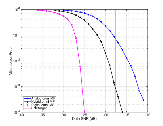
Figure 6: Misdetection Probability vs. data SNR: Omnidirectional transmission and multipath channel. Hybrid beamforming’s performance lies between those of analog and digital BF.

Both analog and digital BF have shortcomings of their own. The lack of multi-direction searching of the former and high power consumption of the latter have lead to a hybrid design that tries to bring a compromise between these two BF strategies [16, 17, 6]. With Hybrid, or quasi-analog BF, (HBF) the detector can “look” in more than one directions while the number of RF chains (A/Ds) are kept lower than the number of antenna elements. Hence, power consumption is lower than digital BF. The number of the required phase shifters, though, is as many as the size of the antenna array times the number of RF chains. Each antenna element will receive/transmit a combination of the directional weights coming from the phase shifters connected to a different RF chain. Due to space limitation, we refrain from going into more details regarding HBF.

We limit our comments on HBF mostly to a comparison of the performance of HBF in detecting the synchronization signal to that of analog and digital BF. Fig. 6, illustrates the performance of the three different detectors, in different SNR regimes. We chose omnidirectionial transmission in multipath as our simulation scenario, since, as we showed earlier, this combination provides the best performance in both analog and digital BF. Also, the number of RF chains in this simulation is set to $4$, resulting into $4$ receiving beams. It can be seen that HBF’s performance lies between those of analog and digital BF. This is expected, since the main factor affecting the performance of the detector is the amount of opportunities it has to align the receiving beam(s) with the strongest incoming path, given a limited search time. HBF has more chances than analog BF (it can “look” in more directions), but less than digital. In this regard, HBF provides a simple method of trading off reduced search time with increased number of digital streams, that may be useful if a fully digital architecture is not feasible.

Conclusions

We have studied directional cell search in a mmWave cellular setting. Two cases are presented: (i) when the base station periodically transmits synchronization signals in random directions to scan the angular space and (ii) when the base station transmits signals omnidirectionally. GLRT detectors are derived for the UE for both analog and digital beamforming. The GLRT detectors are shown to reduce to matched filters with the synchronization signal, with an added eigenvector search in the digital case to locate the optimal receiver spatial signature. Simulations were conducted under realistic parameters, both in single path channels and multipath channels derived from actual field measurements. The simulations indicate that omnidirectional transmission of the synchronization signal performs much better than random angular search in both digital and analog cases. Sequential beam searching remains to be studied. The simulations also show that digital beamforming offers significantly better performance than analog beamforming. In addition, we have argued that increase in power consumption for fully digital front-ends can be compensated by using very low bit rates per antenna with minimal loss in performance. These results suggest that a fully digital front-end with low bit rate per antenna and an appropriate search algorithm may be a fundamentally better design choice for cell search than analog beamforming. One could thus imagine a design where low-rate digital beamforming could be used during cell search, while analog or hybrid beamforming is used for transmissions once the directions are established.

Appendix A Derivation of the GLRT for Digital Beamforming

We wish to show that, for every threshold $t^{\prime}$, the GLRT (6) is equivalent to a test of the form (9). To simplify the notation, throughout this section, we will fix the delay $\tau$ and drop the dependence on $\tau$ on various variables. For example, we will write $\Lambda$ for $\Lambda(\tau)$. In addition, it will be easier to perform all the calculations in a finite-dimensional signal space. To this end, let $W_{k}$ be the signal space containing the signals for the $k$-th PSS time slot, which we will assume has some finite dimension $N$ that is the same for all time slots $k$. Since each PSS time slot has length $T_{sig}$, we can take $N\approx W_{tot}T_{sig}$ where $W_{tot}$ is the total signal bandwidth. Find an orthonormal basis for each $W_{k}$ and for all sub-signals in the the $k$-th time slot. For all sub-signals $p_{\ell}(t)$ transmitted in the $k$-th let $\mathbf{p}_{\ell}\in{\mathbb{C}}^{N}$ be the sub-signal conjugate, $p_{\ell}^{*}(t)$ in the orthonormal basis for the signal space. Similarly, let $\mathbf{R}_{k}\in{\mathbb{C}}^{N_{rx}\times N}$ be a matrix with the $N$ coefficients of the $N_{rx}$ antenna components of the received signal vector $\mathbf{y}(t-\tau)$ in the space $W_{k}$. Similarly, let $\mathbf{D}_{k}\in{\mathbb{C}}^{N_{rx}\times N}$ be the matrix of the coefficients of the noise vector $\mathbf{d}(t)$ in (2). Since $\mathbf{d}(t)$ is Gaussian white noise with PSD $\nu$, the components of $\mathbf{D}_{k}$ will be white Gaussian with variance $\nu$. With these definitions, the two hypotheses (5) can be rewritten in the finite-dimensional signals spaces as

$$H_{1}:~{}\mathbf{R}_{k}=\sum_{\ell\in J_{k}}\alpha_{\ell}\mathbf{u}p_{\ell}^{*}+\mathbf{D}_{k},$$ (21a)

$$H_{0}:~{}\mathbf{R}_{k}=\mathbf{D}_{k},$$ (21b)

where we recall that $J_{k}$ is the subset of indices $\ell$ such that the $\ell$-th subsignal is the space $W_{\ell}$. Let $\mathbf{R}$ be the matrix of the coefficients from all $N_{slot}$ PSS time slots:

$$\mathbf{R}=\left[\mathbf{R}_{1},\cdots,\mathbf{R}_{N_{slot}}\right].$$ (22)

Since there is a one-to-one mapping between the continuous-time delay data $\mathbf{Y}_{\tau}$ and the coefficients in the signal space $\mathbf{R}$, we can rewrite the GLRT (6) in terms of $\mathbf{R}$ instead of $\mathbf{Y}_{\tau}$:

$$\Lambda:=\log\frac{\max_{{\bm{\theta}}}p(\mathbf{R}|H_{1},{\bm{\theta}})}{\max_{{\bm{\theta}}}p(\mathbf{R}|H_{0},{\bm{\theta}})}\underset{H_{0}}{\overset{H_{1}}{\gtrless}}\;t^{\prime}$$ (23)

where $p(\mathbf{R}|H_{i},{\bm{\theta}})$ is the density of the received data $\mathbf{R}$ under the hypothesis $H_{0}$ or $H_{1}$ and parameters ${\bm{\theta}}$.

Now, since the noise matrices $\mathbf{D}_{k}$ in (21) are independent, the log likelihood ratio (23) factors as

$$\Lambda=\min_{\nu}\sum_{k=1}^{N_{slot}}\Lambda^{0}_{k}(\nu)-\min_{\nu,\mathbf{u}}\sum_{k=1}^{N_{slot}}\Lambda^{1}_{k}(\nu,\mathbf{u}),$$ (24)

where $\Lambda^{i}_{k}(\nu,\mathbf{u})$ are the negative log likelihoods for the data $\mathbf{R}_{k}$ for each PSS time slot $k$:

$$\Lambda^{0}_{k}(\nu) = -\log p(\mathbf{R}_{k}|H_{0},\nu)$$ (25a)

$$\Lambda^{1}_{k}(\nu,\mathbf{u}) = \min_{{\bm{\alpha}}_{k}}\left[-\log p(\mathbf{R}_{k}|H_{1},\nu,\mathbf{u},{\bm{\alpha}}_{k})\right],$$ (25b)

where ${\bm{\alpha}}_{k}$ is the vector of the channel gains $\alpha_{\ell}$ for the sub-signals $\ell$ in the $k$-th time slot,

$${\bm{\alpha}}_{k}=\left\{\alpha_{\ell},\ell\in J_{k}\right\}.$$

Note that, in the $H_{0}$ hypothesis, there is no dependence on the parameters $\mathbf{u}$ and ${\bm{\alpha}}_{k}$. Now, given $\mathbf{u}$ and $\nu$, the coefficients in $\mathbf{R}_{k}$ in (21) are complex Gaussians with $M:=NN_{rx}$ independent components. Hence, the likelihoods (25) are given by

$$\Lambda^{0}_{k}(\nu)=\frac{1}{\nu}\|\mathbf{R}_{k}\|^{2}_{F}+M\log(2\pi\nu)$$ (26a)

$$\Lambda^{1}_{k}(\nu,\mathbf{u})=M\log(2\pi\nu)$$ (26b)

$$+ \frac{1}{\nu}\min_{{\bm{\alpha}}_{k}}\|\mathbf{R}_{k}-\sum_{\ell\in J_{k}}\alpha_{\ell}\mathbf{u}\mathbf{p}_{\ell}^{*}\|^{2}_{F}.$$

Since we have assumed that the different sub-signals $p_{\ell}(t)$ are orthogonal, the vector representations $\mathbf{p}_{\ell}$ will also be orthogonal. Hence, the minimization in (26b) is given by

$$\Lambda^{1}_{k}(\nu,\mathbf{u})=M\log(2\pi\nu)$$ (27)

$$+ \frac{1}{\nu}\left[\|\mathbf{R}_{\ell}\|^{2}_{F}-\sum_{\ell\in J_{k}}\frac{|\mathbf{u}^{*}\mathbf{R}_{k}\mathbf{p}_{\ell}|^{2}}{\|\mathbf{p}_{\ell}\|^{2}\|\mathbf{u}\|^{2}}\right].$$

We next compute the minimizations over $\nu$ and $\mathbf{u}$. For the $H_{0}$ hypothesis, we apply (26a) to obtain

$$\min_{\nu}\sum_{k=1}^{N_{slot}}\Lambda^{0}_{k}(\nu)=\min_{\nu}\sum_{k=1}^{N_{slot}}\left[\frac{1}{\nu}\|\mathbf{R}_{k}\|^{2}_{F}+M\log(2\pi\nu)\right]$$ (28)

$$= \min_{\nu}\left[\frac{1}{\nu}\|\mathbf{R}\|^{2}_{F}+N_{slot}M\log(2\pi\nu)\right]$$

$$= N_{slot}M+N_{slot}M\log\left[\frac{2\pi}{N_{slot}M}\|\mathbf{R}\|^{2}_{F}\right],\hskip 56.9055pt$$

where we have used the fact that

$$\|\mathbf{R}\|^{2}_{F}=\sum_{k=1}^{N_{slot}}\|\mathbf{R}_{k}\|^{2}_{F}.$$ (29)

For the $H_{1}$ hypothesis, first observe that

$$\sum_{k=1}^{N_{slot}}\left\{\|\mathbf{R}_{k}\|^{2}_{F}-\sum_{\ell\in J_{k}}\frac{|\mathbf{u}^{*}\mathbf{R}_{k}\mathbf{p}_{\ell}|^{2}}{\|\mathbf{p}_{\ell}\|^{2}\|\mathbf{u}\|^{2}}\right\}$$ (30)

$$\stackrel{{\scriptstyle(a)}}{{=}} \sum_{k=1}^{N_{slot}}\|\mathbf{R}_{k}\|^{2}_{F}-\sum_{\ell=1}^{L}\frac{|\mathbf{u}^{*}\mathbf{R}_{\sigma(\ell)}\mathbf{p}_{\ell}|^{2}}{\|\mathbf{p}_{\ell}\|^{2}\|\mathbf{u}\|^{2}}$$

$$\stackrel{{\scriptstyle(b)}}{{=}} \|\mathbf{R}\|^{2}_{F}-\frac{\|\mathbf{u}^{*}\mathbf{V}\|^{2}}{\|\mathbf{u}\|^{2}},$$

where in step (a), we have used the notation that $\sigma(\ell)$ is the index $k$ for the PSS time-slot in which the sub-signal $p_{\ell}(t)$ is transmitted. In step (b), we have again used (29) and re-written the sum over $\ell$ using a matrix $\mathbf{V}$ defined as

$$\mathbf{V}=\left[\frac{1}{\|\mathbf{p}_{1}\|}\mathbf{R}_{\sigma(1)}\mathbf{p}_{1},\cdots,\frac{1}{\|\mathbf{p}_{L}\|}\mathbf{R}_{\sigma(L)}\mathbf{p}_{L}\right].$$ (31)

The minimum of (30) over $\mathbf{u}$ is given by the maximum singular value [25]:

$$\min_{\mathbf{u}}\|\mathbf{R}\|^{2}_{F}-\frac{\|\mathbf{u}^{*}\mathbf{V}\|^{2}}{\|\mathbf{u}\|^{2}}=\|\mathbf{R}\|^{2}_{F}-\sigma_{max}^{2}(\mathbf{V}),$$ (32)

Substituting (30) and (32) into (27) we obtain

$$\min_{\nu,\mathbf{u}}\sum_{\ell=1}^{L}\Lambda^{1}_{\ell}(\nu,\mathbf{u})$$ (33)

$$= \min_{\nu}\frac{1}{\nu}\left[\|\mathbf{R}\|^{2}_{F}-\sigma_{max}^{2}(\mathbf{V})\right]+N_{slot}M\log(2\pi\nu)$$

$$= N_{slot}M$$

$$+N_{slot}M\log\left[\frac{2\pi}{N_{slot}M}(\|\mathbf{R}\|^{2}_{F}-\sigma_{max}^{2}(\mathbf{V}))\right].$$

Substituting (28) and (33) into (24), we see that the GLRT is given by

$$\Lambda=-N_{slot}M\log\left[1-\frac{\sigma^{2}_{max}(\mathbf{V})}{\|\mathbf{R}\|^{2}_{F}}\right]$$ (34)

$$= -N_{slot}M\log\left[(1-T)\right],$$

where $T$ is the statistic,

$$T:=\frac{\sigma^{2}_{max}(\mathbf{V})}{\|\mathbf{R}\|^{2}_{F}}.$$ (35)

Since $\Lambda$ is an increasing function of the statistic $T$, a ratio test (23) is equivalent to a test of the form

$$T\underset{H_{0}}{\overset{H_{1}}{\gtrless}}\;t.$$

It remains to show that the statistic $T$ in (35) is identical to $T(\tau)$ in (9). To this end, first recall that the matrices $\mathbf{R}_{k}$ are the coefficients of the received signal $\mathbf{y}(t-\tau)$ in the signal space for the time slot $I_{k}$. Since the coefficients are in an orthonormal basis, the energy is preserved so that

$$\|\mathbf{R}_{k}\|^{2}_{F}=\int_{t\in I_{k}+\tau}\|\mathbf{y}(t)\|^{2}dt=\int_{I_{k}}\|\mathbf{y}(t-\tau)\|^{2}dt.$$

Therefore, the energy $E(\tau)$ in (8) is given by

$$E(\tau)=\sum_{k=1}^{N_{slot}}\|\mathbf{R}_{k}\|^{2}_{F}=\|\mathbf{R}\|_{F}^{2}.$$ (36)

Similarly, for every $\ell\in J_{k}$, $\mathbf{p}_{\ell}$ is the vector representation of the sub-signal $p_{\ell}^{*}(t)$ in the signal space for the $k$-th PSS time slot. Since we are using an orthonormal basis, $\mathbf{R}_{k}\mathbf{p}_{\ell}$ must be inner product,

$$\mathbf{R}_{k}\mathbf{p}_{\ell}=\int_{I_{k}}\mathbf{y}(t-\tau)p_{\ell}^{*}(t)dt=\int\mathbf{y}(t-\tau)p_{\ell}^{*}(t)dt,$$

where the last step is valid since the support of $p_{\ell}(t)$ is contained in the interval $I_{k}$. Therefore, the normalized correlation $\mathbf{v}_{\ell}(\tau)$ is precisely

$$\mathbf{v}(\tau)=\frac{1}{\|\mathbf{p}_{\ell}\|}\mathbf{R}_{k}\mathbf{p}_{\ell}.$$

This identity implies that the matrix $\mathbf{V}(\tau)$ in (10) is precisely (31). Combining this fact with (36) shows that statistic $T$ in (35) is identical to $T(\tau)$ in (9). We conclude that the GLRT (6) is equivalent to the correlation test (9).

Appendix B Derivation of the GLRT for Analog Beamforming

Similar to the previous section, we prove that for every threshold $t^{\prime}$, the GLRT (13) is equivalent to a test of the form (15). Again, the dependence on $\tau$ is dropped to simplify the notation. As before, we use a finite dimensional signal space representation for all the signals. Let $\mathbf{r}_{k}\in{\mathbb{C}}^{N}$ be the vector representation of the delayed beamformed signal $z(t-\tau)$ in the signal space $W_{k}$ for the $k$-th PSS time slot. Similarly, let $\mathbf{d}_{k}$ and $\mathbf{p}_{\ell}\in{\mathbb{C}}^{N}$ be the representation for the noise signal $d(t)$ and PSS sub-signal $p_{\ell}(t)$. Then, the two hypotheses (11) can be re-written as

$$H_{1}:~{}\mathbf{r}_{k}=\sum_{\ell\in J_{k}}\beta_{\ell}\mathbf{p}_{\ell}+\mathbf{d}_{k},$$ (37a)

$$H_{0}:~{}\mathbf{r}_{k}=\mathbf{d}_{k},$$ (37b)

Let $\mathbf{R}$ be the matrix of the data for all the time slots

$$\mathbf{R}=\left[\mathbf{r}_{1},\cdots,\mathbf{r}_{N_{slot}}\right].$$

The GLRT (13) can then be re-written as

$$\Lambda:=\log\frac{\max_{{\bm{\theta}}}p(\mathbf{R}|H_{1},{\bm{\theta}})}{\max_{{\bm{\theta}}}p(\mathbf{R}|H_{0},{\bm{\theta}})}\underset{H_{0}}{\overset{H_{1}}{\gtrless}}\;t^{\prime}$$ (38)

where $p(\mathbf{R}|H_{i},{\bm{\theta}})$ is the density of the received data $\mathbf{R}$ under the hypothesis $H_{0}$ or $H_{1}$ and parameters ${\bm{\theta}}$.

As before, the likelihood ratio in (38) factors as:

$$\Lambda=\min_{\nu}\sum_{k=1}^{N_{slot}}\Lambda^{0}_{k}(\nu)-\min_{\nu}\sum_{k=1}^{N_{slot}}\Lambda^{1}_{k}(\nu),$$ (39)

where $\Lambda^{i}_{k}(\nu)$ are the negative log likelihoods for the data $\mathbf{r}_{k}$ for each sub-signal $k$:

$$\Lambda^{0}_{k}(\nu) = -\log p(\mathbf{r}_{k}|H_{0},\nu)$$ (40a)

$$\Lambda^{1}_{k}(\nu) = \min_{{\bm{\beta}}_{k}}\left[-\log p(\mathbf{r}_{\ell}|H_{1},\nu,{\bm{\beta}}_{k})\right],$$ (40b)

where ${\bm{\beta}}_{k}$ is the vector of channel gains for the $k$-th time slot

$${\bm{\beta}}_{k}=\left\{\beta_{\ell}~{}|~{}\ell\in J_{k}\right\}.$$

We know that the noise vector $\mathbf{d}_{k}$ in (37) is a vector of length $N$ consisting of independent complex gaussian random variables. Hence, using the hypothesis models (37), the likelihoods in (40) are equal to:

$$\Lambda^{0}_{k}(\nu)=\frac{1}{\nu}\|\mathbf{r}_{k}\|^{2}+N\log(2\pi\nu)$$ (41a)

$$\Lambda^{1}_{k}(\nu)=N\log(2\pi\nu)$$ (41b)

$$+ \frac{1}{\nu}\min_{{\bm{\beta}}_{k}}\|\mathbf{r}_{k}-\sum_{\ell\in J_{k}}\beta_{\ell}\mathbf{p}_{\ell}\|^{2}.$$

Since the vectors $\mathbf{p}_{\ell}$ are orthogonal, the minimization in (41b) is given by

$$\Lambda^{1}_{k}(\nu)=N\log(2\pi\nu)$$ (42)

$$+ \frac{1}{\nu}\left[\|\mathbf{r}_{k}\|^{2}-\sum_{\ell\in J_{k}}\frac{|\mathbf{r}_{k}^{*}\mathbf{p}_{\ell}|^{2}}{\|\mathbf{p}_{\ell}\|^{2}}\right].$$

Next, we perform the minimizations of both hypotheses over $\nu$. For the $H_{0}$ hypothesis, we have:

$$\min_{\nu}\sum_{k=1}^{N_{slot}}\Lambda^{0}_{k}(\nu)=\min_{\nu}\sum_{k=1}^{N_{slot}}\left[\frac{1}{\nu}\|\mathbf{r}_{k}\|^{2}+N\log(2\pi\nu)\right]$$ (43)

$$= \min_{\nu}\left[\frac{1}{\nu}\|\mathbf{r}\|^{2}+NN_{slot}\log(2\pi\nu)\right]$$

$$= NN_{slot}+NN_{slot}\log\left[\frac{2\pi}{NN_{slot}}\|\mathbf{r}\|^{2}\right],\hskip 56.9055pt$$

where we have used the fact that

$$\|\mathbf{r}\|^{2}=\sum_{k=1}^{N_{slot}}\|\mathbf{r}_{k}\|^{2}.$$ (44)

For the $H_{1}$ case, we first evaluate the summation over the slots,

$$\sum_{k=1}^{N_{slot}}\left\{\|\mathbf{r}_{k}\|^{2}-\sum_{\ell\in J_{k}}\frac{|\mathbf{r}_{k}^{*}\mathbf{p}_{\ell}|^{2}}{\|\mathbf{p}_{\ell}\|^{2}}\right\}$$ (45)

$$\stackrel{{\scriptstyle(a)}}{{=}} \sum_{k=1}^{N_{slot}}\|\mathbf{r}_{k}\|^{2}-\sum_{\ell=1}^{L}\frac{|\mathbf{r}_{\sigma(\ell)}^{*}\mathbf{p}_{\ell}|^{2}}{\|\mathbf{p}_{\ell}\|^{2}}$$

$$\stackrel{{\scriptstyle(b)}}{{=}} \|\mathbf{r}\|^{2}-\|\mathbf{v}\|^{2},$$

where in step (a), as before, we have used the notation that $\sigma(\ell)$ is the index $k$ for the PSS time-slot in which the sub-signal $p_{\ell}(t)$ is transmitted. In step (b), we have again used (44) and re-written the sum over $\ell$ using the vector $\mathbf{v}$ defined as

$$\mathbf{v}=\left[\frac{1}{\|\mathbf{p}_{1}\|}\mathbf{r}_{\sigma(1)}^{*}\mathbf{p}_{1},\cdots,\frac{1}{\|\mathbf{p}_{L}\|}\mathbf{r}_{\sigma(L)}^{*}\mathbf{p}_{L}\right].$$ (46)

Combining (42) and (45), we obtain:

$$\min_{\nu}\sum_{k=1}^{N_{slot}}\Lambda^{1}_{k}(\nu)$$ (47)

$$= \min_{\nu}\left\{NN_{slot}\log(2\pi\nu)+\frac{1}{\nu}(\|\mathbf{r}\|^{2}-\|\mathbf{v}\|^{2})\right\}$$

$$= NN_{slot}+NN_{slot}\log\left[\frac{2\pi}{NN_{slot}}(\|\mathbf{r}\|^{2}-\|\mathbf{v}\|^{2})\right].$$

Substituting (47) and (43) into (39), the GLRT is given by:

$$\Lambda=-NN_{slot}\log\left[\left(1-\frac{\|\mathbf{v}\|^{2}}{\|\mathbf{r}\|^{2}}\right)\right]$$ (48)

$$= -NN_{slot}\log\left[(1-T)\right],$$

where $T$ is the statistic,

$$T=\frac{\|\mathbf{v}\|^{2}}{\|\mathbf{r}\|^{2}}.$$ (49)

As before, we can conclude that since $\Lambda$ is an increasing function of $T$, for every threshold level $t^{\prime}$, the ratio test given by (38) is equivalent to a test of the form

$$T\underset{H_{0}}{\overset{H_{1}}{\gtrless}}\;t,$$ (50)

for some threshold level $t$. With a similar argument to the digital beamforming case, we can show that the $T$ defined in (49) is precisely the test statistic $T(\tau)$ in (15). We conclude that the GLRT in (13) is equivalent to a correlation threshold test (15).

Appendix C Simulation Parameter Selection Details

In this section, we provide more details on the logic behind the selection of their simulation parameters, and also illustrate some of the considerations that should be made in selecting these values for practical systems.

Signal parameters

As mentioned in Section II, the synchronization signal is divided into $N_{sig}$ narrow-band sub-signals sent over different frequency bands to provide frequency diversity. Our experiments indicated that $N_{sig}=4$ provides a good tradeoff between frequency diversity and coherent combining. However, due to space, we do not report the results for other values of $N_{sig}$. For the length of the PSS interval, we took $T_{sig}=$ 100 $\mu s$, which is sufficiently small that the channel will be coherent even at the very high frequencies for mmWave. For example, at a UE with velocity of $30$ kmph and 28 GHz, the maximum Doppler shift of the mmWave channel is $\approx 780$ Hz, so the coherence time is $\gg 100~{}\mu$s. Measurements of typical delay spreads in a mmWave outdoor setting indicate delay spreads within a narrow angular region to be typically less $<30\;\text{ns}$ [26, 29]. This means that if we take the sub-signal bandwidth of $W_{sig}$ = 1 MHz, the channel will be relatively flat across this band.

Now, since the PSS signals occur every $T_{per}$ seconds, the PSS overhead will be $T_{sig}/T_{per}$. With our parameter selection, the overhead of the signal is $2$%. In fact, any $T_{per}$ greater than $5$ ms gives us an overhead less than 2%.

False alarm target

To set an appropriate false alarm target, we recognize that false alarms on the PSS result in additional searches for a secondary synchronization signal (SSS), which costs both computational power and increases the false alarm rate for the SSS. The precise acceptable level for the PSS false alarm rate will depend on the SSS signal design. In this simulation, we will assume that the total false alarm rate is at most $R_{FA}$ = 0.01 false alarm per search period. Thus, the false alarm rate per delay hypothesis must be $P_{FA}\leq R_{FA}/(N_{hyp})$ where $N_{hyp}$ is the number of hypotheses that will be tested per second. The number of hypotheses are given by the product

$$N_{hyp}=N_{dly}N_{PSS}N_{FO},$$

where $N_{dly}$ is the number of delay hypotheses per transmission period $T_{per}$, $N_{PSS}$ is the number of PSS waveforms that can be transmitted by the base station and $N_{FO}$ is the number of frequency offsets. The values for these will depend on whether the UE is performing the cell search for initial access or while in connected mode for handover. In this paper, we consider only the initial access case.

For initial access, the UE must search over delays in the range $\tau\in[0,T_{per}]$. Assuming the correlations are computed at twice the bandwidth, we will have $N_{dly}=2W_{sig}T_{per}=2(10)^{6}\times 5(10)^{-3}=10^{4}$. For the number of PSS signals, we will take $N_{PSS}=3$, which is same as the number of signals offered by the current LTE system. However, we may need to increase this number to accommodate more cell IDs in a dense BS deployment. To estimate the number of frequency offsets, suppose that the initial frequency offset can be as much as 1 ppm at 28 GHz. This will result in an frequency offset of $28(10)^{3}$ Hz. The maximum Doppler shift will add approximately 780 Hz, giving a total initial frequency offset error of $\Delta f_{max}=28+0.78$ kHz. In order that the channel does not rotate more than 90^∘ over the period of $T_{sig}=100$ $\mu$s, we need a frequency accuracy of $\Delta f=10^{4}/4$. Since $2\Delta f_{max}/\Delta f=23.0$, it will suffice to take $N_{FO}=23$ frequency offset hypotheses. Hence, the target FA rate for initial access should be

$$P_{FA}=\frac{R_{FA}}{N_{hyp}}=\frac{0.01}{10^{4}(3)23}=1.4493(10)^{-8}.$$

Antenna pattern

We assume a set of two dimensional antenna arrays at both the BS and the UE. On the BS side, the array is comprised of $8\times 8$ elements and on the receiver side we have $4\times 4$ elements. The spacing of the elements is set at $\lambda/2$, where $\lambda$ is the wavelength. These antenna patterns were considered in [8] and showed to offer excellent system capacity for small cell urban deployments. In addition, a $4\times 4$ array operating in the $28\;\text{GHz}$ band, for instance, will have dimensions of roughly $1.5\;\text{cm}\times 1.5\;\text{cm}$.

Appendix D Quantization Effects

To estimate the effect of quantization, we use a standard AWGN model for the quantization noise [22]. Let $r[n]$ be the complex samples of some signal that we model as a random process of the form,

$$r[n]=x[n]+w[n],\quad E|x[n]|^{2}=E_{s},~{}E|w[n]|^{2}=N_{0},$$ (51)

where $x[n]$ represents the signal, $w[n]$ is the noise, and $E_{s}$ and $N_{0}$ are the signal and noise energy per sample. The SNR of this signal is

$$\gamma_{0}=E_{s}/N_{0}.$$

Now consider a quantized version of this signal, $\widehat{r}[n]=Q(r[n])$ where $Q(\cdot)$ is a scalar quantizer applied to each sample. It is shown in [32] that the quantizer can be modeled as

$$\widehat{r}[n]=Q(r[n])=(1-\alpha)r[n]+v[n],$$ (52)

where $v[n]$ is quanitization noise that is uncorrelated with $r[n]$ and has variance

$$E|v[n]|^{2}=\alpha(1-\alpha)E|r[n]|^{2}=\alpha(1-\alpha)(E_{s}+N_{0}).$$ (53)

In (52) and (53), $\alpha$ is the relative quantization error (or inverse coding gain using the terminology in [22]),

$$\alpha:=\frac{E|Q(r)-r|^{2}}{E|r|^{2}}.$$

This relative error is a function of the number of bits of the quantizer, the choice of the quantizer levels and the distribution of the quantizer input. Table II shows the values for $\alpha$ (in dB scale) for various bit values for a simple scalar uniform quantizer with Gaussian input. For the values in the table, a simple numerical optimization is run to optimize the step size to obtain the minimum relative error $\alpha$. In practice, the actual signal level will not arrive at the optimal level due to imperfections in the A/D – so a few more bits are likely needed.

Substituting (51) into (52), we obtain

$$\widehat{r}[n]=Q(r[n])=(1-\alpha)x[n]+(1-\alpha)w[n]+v[n].$$

Hence, the effective SNR after quantization is

$$\gamma=\frac{(1-\alpha)^{2}E|x[n]|^{2}}{(1-\alpha)^{2}E|w[n]|^{2}+E|v[n]|^{2}}$$

$$= \frac{(1-\alpha)^{2}E_{s}}{(1-\alpha)^{2}N_{0}+\alpha(1-\alpha)(E_{s}+N_{0})}$$

$$= \frac{(1-\alpha)\gamma_{0}}{1+\alpha\gamma_{0}}.$$

For the PSS detection, suppose that the PSS signal arrives at power $P$ and the noise has a power spectral density $N_{0}$. Since the PSS arrives in $N_{sig}$ sub-signals each having bandwidth $W_{sig}$, the energy per orthogonal sample will be

$$E_{s}=P/(W_{sig}N_{sig})$$

and hence the SNR will be

$$\gamma_{0}=P/N_{0}=P/(W_{sig}N_{sig}N_{0}).$$

Number bits	Coding gain, $-10\log_{10}(\alpha)$ (dB)
1	4.4
2	9.3
3	14.5

TABLE II: Coding gain values as a function of the number of bits for a scalar uniform quantizer with Gaussian noise and an optimized step size.

References

- [1] F. Khan and Z. Pi, “An introduction to millimeter-wave mobile broadband systems,” IEEE Comm. Mag., vol. 49, no. 6, pp. 101 – 107, Jun. 2011.
- [2] P. Pietraski, D. Britz, A. Roy, R. Pragada, and G. Charlton, “Millimeter wave and terahertz communications: Feasibility and challenges,” ZTE Communications, vol. 10, no. 4, pp. 3–12, Dec. 2012.
- [3] T. S. Rappaport, S. Sun, R. Mayzus, H. Zhao, Y. Azar, K. Wang, G. N. Wong, J. K. Schulz, M. Samimi, and F. Gutierrez, “Millimeter Wave Mobile Communications for 5G Cellular: It Will Work!” IEEE Access, vol. 1, pp. 335–349, May 2013.
- [4] S. Rangan, T. S. Rappaport, and E. Erkip, “Millimeter-wave cellular wireless networks: Potentials and challenges,” Proceedings of the IEEE, vol. 102, no. 3, pp. 366–385, March 2014.
- [5] J. Andrews, S. Buzzi, W. Choi, S. Hanly, A. Lozano, A. Soong, and J. Zhang, “What will 5G be?” IEEE JSAC on 5G Wireless Communication Systems, vol. 32, no. 6, pp. 1065–1082, June 2014.
- [6] A. Ghosh, T. A. Thomas, M. C. Cudak, R. Ratasuk, P. Moorut, F. W. Vook, T. S. Rappaport, G. MacCartney, S. Sun, and S. Nie, “Millimeter wave enhanced local area systems: A high data rate approach for future wireless networks,” Selected Areas in Communications, IEEE Journal on, vol. 32, no. 6, pp. 1152–1163, June 2014.
- [7] T. S. Rappaport, Wireless Communications: Principles and Practice, 2nd ed. Upper Saddle River, NJ: Prentice Hall, 2002.
- [8] M. Akdeniz, Y. Liu, M. Samimi, S. Sun, S. Rangan, T. Rappaport, and E. Erkip, “Millimeter wave channel modeling and cellular capacity evaluation,” IEEE J. Sel. Areas Comm., vol. 32, no. 6, pp. 1164–1179, June 2014.
- [9] T. S. Rappaport, R. W. Heath, R. C. Daniels, and J. N. Murdock, Millimeter Wave Wireless Communications, 1st ed. Prentice Hall, Sep. 2014.
- [10] 3GPP, “Evolved Universal Terrestrial Radio Access (E-UTRA) and Evolved Universal Terrestrial Radio Access Network (E-UTRAN); Overall description; Stage 2,” TS 36.300 (release 10), 2010.
- [11] Q. Li, H. Niu, G. Wu, and R. Q. Hu, “Anchor-booster based heterogeneous networks with mmwave capable booster cells,” in Proc. IEEE Globecom Workshop, Dec. 2013.
- [12] F. Khan and Z. Pi, “Millimeter-wave Mobile Broadband (MMB): Unleashing 3-300GHz Spectrum,” in Proc. IEEE Sarnoff Symposium, Mar. 2011.
- [13] K.-J. Koh and G. M. Rebeiz, “0.13- m CMOS phase shifters for X-, Ku- and K-band phased arrays,” IEEE J. Solid-State Circuts, vol. 42, no. 11, pp. 2535–2546, Nov. 2007.
- [14] ——, “A Millimeter-Wave (40–45 GHz) 16-Element Phased-Array Transmitter in 0.18-m SiGe BiCMOS Technology,” IEEE J. Solid-State Circuts, vol. 44, no. 5, pp. 1498–1509, May 2009.
- [15] X. Guan, H. Hashemi, and A. Hajimiri, “A fully integrated 24-GHz eight-element phased-array receiver in silicon,” IEEE J. Solid-State Circuts, vol. 39, no. 12, pp. 2311–2320, Dec. 2004.
- [16] A. Alkhateeb, O. E. Ayach, G. Leus, and J. Robert W. Heath, “Hybrid precoding for millimeter wave cellular systems with partial channel knowledge,” in Proc. Information Theory and Applications Workshop (ITA), Feb. 2013.
- [17] S. Sun, T. Rappaport, R. Heath, A. Nix, and S. Rangan, “Mimo for millimeter-wave wireless communications: beamforming, spatial multiplexing, or both?” Communications Magazine, IEEE, vol. 52, no. 12, pp. 110–121, December 2014.
- [18] H. L. Van Trees, Detection, Estimation and Modulation Theory, Part I. New York, NY: Wiley, 2001.
- [19] H. Zhang, S. Venkateswaran, and U. Madhow, “Analog multitone with interference suppression: Relieving the ADC bottleneck for wideband 60 GHz systems,” in Proc. IEEE Globecom, Nov. 2012.
- [20] D. Ramasamy, S. Venkateswaran, and U. Madhow, “Compressive tracking with 1000-element arrays: a framework for multi-gbps mm wave cellular downlinks,” in Proc. 50th Ann. Allerton Conf. on Commun., Control and Comp., Monticello, IL, Sep. 2012.
- [21] K. Hassan, T. Rappaport, and J. Andrews, “Analog equalization for low power 60 GHz receivers in realistic multipath channels,” in Proc. IEEE Globecom, Dec 2010, pp. 1–5.
- [22] A. Gersho and R. M. Gray, Vector Quantization and Signal Compression. Boston, MA: Kluwer Acad. Pub., 1992.
- [23] C. N. Barati, S. A. Hosseini, S. Rangan, P. Liu, T. Korakis, and S. S. Panwar, “Directional cell search for millimeter wave cellular systems,” in Proc. IEEE SPAWC, Toronto, Canada, Jun. 2014.
- [24] E. Dahlman, S. Parkvall, J. Sköld, and P. Beming, 3G Evolution: HSPA and LTE for Mobile Broadband. Oxford, UK: Academic Press, 2007.
- [25] G. H. Golub and C. F. V. Loan, Matrix Computations, 2nd ed. Baltimore, MD: Johns Hopkins Univ. Press, 1989.
- [26] Y. Azar, G. N. Wong, K. Wang, R. Mayzus, J. K. Schulz, H. Zhao, F. Gutierrez, D. Hwang, and T. S. Rappaport, “28 GHz propagation measurements for outdoor cellular communications using steerable beam antennas in New York City,” in Proc. IEEE ICC, 2013.
- [27] H. Zhao, R. Mayzus, S. Sun, M. Samimi, J. K. Schulz, Y. Azar, K. Wang, G. N. Wong, F. Gutierrez, and T. S. Rappaport, “28 GHz millimeter wave cellular communication measurements for reflection and penetration loss in and around buildings in New York City,” in Proc. IEEE ICC, 2013.
- [28] M. Samimi, K. Wang, Y. Azar, G. N. Wong, R. Mayzus, H. Zhao, J. K. Schulz, S. Sun, F. Gutierrez, and T. S. Rappaport, “28 GHz angle of arrival and angle of departure analysis for outdoor cellular communications using steerable beam antennas in New York City,” in Proc. IEEE VTC, 2013.
- [29] G. R. MacCartney, M. K. Samimi, and T. S. Rappaport, “Exploiting directionality for millimeter-wave system improvement,” in International Conference on Communications (ICC) (submitted), 2015 IEEE, Jun 2015.
- [30] M. K. Samimi and T. S. Rappaport, “3-d statistical channel models for millimeter-wave outdoor mobile broadband communications,” in International Conference on Communications (ICC) (submitted), 2015 IEEE, Jun 2015.
- [31] V. Chen and L. Pileggi, “An 8.5mw 5gs/s 6b flash adc with dynamic offset calibration in 32nm cmos soi,” Jun. 2013, pp. C264–C265.
- [32] A. K. Fletcher, S. Rangan, V. K. Goyal, and K. Ramchandran, “Robust predictive quantization: Analysis and design via convex optimization,” IEEE J. Sel. Topics Signal Process., vol. 1, no. 4, pp. 618–632, Dec. 2007.