Clustering via Mode Seeking by Direct Estimation of the Gradient of a Log-Density

Abstract

Mean shift clustering finds the modes of the data probability density by identifying the zero points of the density gradient. Since it does not require to fix the number of clusters in advance, the mean shift has been a popular clustering algorithm in various application fields. A typical implementation of the mean shift is to first estimate the density by kernel density estimation and then compute its gradient. However, since good density estimation does not necessarily imply accurate estimation of the density gradient, such an indirect two-step approach is not reliable. In this paper, we propose a method to directly estimate the gradient of the log-density without going through density estimation. The proposed method gives the global solution analytically and thus is computationally efficient. We then develop a mean-shift-like fixed-point algorithm to find the modes of the density for clustering. As in the mean shift, one does not need to set the number of clusters in advance. We empirically show that the proposed clustering method works much better than the mean shift especially for high-dimensional data. Experimental results further indicate that the proposed method outperforms existing clustering methods.

1 Introduction

Seeking the modes of a probability density has led to a powerful clustering algorithm called the mean shift [7, 9, 12]. In the mean shift algorithm, all input samples are initially regarded as candidates of the modes of the density and they are iteratively updated and merged. Finally, clustering is performed by associating the input samples with the obtained modes. An advantage of the mean shift is that the number of clusters does not need to be specified in advance. Thanks to this extremely useful property, the mean shift has been successfully employed in various applications such as image segmentation [9, 25, 27] and object tracking [8, 10].

In mode seeking, a central technical challenge is accurate estimation of the gradient of a density. The mean shift takes a two-step approach: kernel density estimation (KDE) is first used to approximate the density and then its gradient is computed. However, such a two-step approach performs poorly because a good estimator of the density does not necessarily mean a good estimator of the density gradient. In particular, KDE tends to produce a smooth density estimate and therefore the density is over-flattened. This yields the modes in a multi-modal density to be collapsed. Furthermore, KDE itself tends to perform poorly in high-dimensional problems [9].

To overcome this problem, we propose a method called least-squares log-density gradients (LSLDG), which directly estimates the gradient of a log-density by least-squares without going through density estimation. The proposed method can be regarded as a non-parametric extension of score matching [15, 22], which has originally been developed for least-squares parametric density estimation with intractable partition functions. We then derive a fixed-point algorithm to find the modes of the density, which is our proposed clustering algorithm called LSLDG clustering.

All tuning parameters included in LSLDG such as the Gaussian kernel width and the regularization parameter can be objectively optimized by cross-validation in terms of the squared error. Furthermore, since LSLDG clustering inherits the same algorithmic structure as the original mean shift, it does not require the number of clusters to be fixed in advance. Thus, LSLDG clustering does not involve any tuning parameters to be manually determined, which is a significant advantage over standard clustering algorithms such as spectral clustering [20], because clustering is an unsupervised learning problem and appropriately controlling tuning parameters is generally very hard. A recent study based on information-maximization clustering [23] provided an information-theoretic mean to determine tuning parameters objectively, but it still requires the user to fix the number of clusters in advance.

The remainder of this paper is structured as follows. We derive a method to directly estimate the gradient of a log-density in Section 2, and then use it for finding clusters in the data in Section 3. Various possibilities for extension are discussed in Section 4, and the usefulness of the proposed method is experimentally investigated in Section 5. Finally this paper is concluded in Section 6.

2 Direct Estimation of the Gradient of a Log-density

In this section, we propose a method to estimate the log-density gradient.

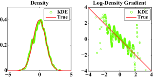
Figure 1: An example of a good density estimation, but inaccurate estimation of the log-density gradient by KDE.

2.1 Problem Formulation

Let us consider a probability distribution on $\mathbb{R}^{d}$ with density $p^{*}(\boldsymbol{x})$, which is unknown but $n$ i.i.d. samples $\mathcal{X}=\{\boldsymbol{x}_{i}\}_{i=1}^{n}$ are available. Our goal is to estimate the gradient of the logarithm of the density $p^{*}(\boldsymbol{x})$ with respect to $\boldsymbol{x}$ from $\mathcal{X}$:

$$\boldsymbol{g}^{*}(\boldsymbol{x})=(g_{1}^{*}(\boldsymbol{x}),\ldots,g_{d}^{*}(\boldsymbol{x}))^{\top}=\nabla\log p^{*}(\boldsymbol{x})=\frac{\nabla p^{*}(\boldsymbol{x})}{p^{*}(\boldsymbol{x})}.$$

A naive approach to estimate $\boldsymbol{g}^{*}(\boldsymbol{x})$ is to first obtain a density estimate $\widehat{p}(\boldsymbol{x})$ and then compute its log-gradient $\nabla\log\widehat{p}(\boldsymbol{x})$. However, this two-step approach does not work well because a good density estimate $\widehat{p}(\boldsymbol{x})$ does not necessarily provide an accurate estimate of its log-gradient $\nabla\log\widehat{p}(\boldsymbol{x})$. For example, in Figure 1, density estimation is performed fairly well, but its log-density gradient is quite inaccurate. Below, we describe a method to directly estimate the log-density gradient $\nabla\log p^{*}(\boldsymbol{x})$ without going through density estimation. The method is based on the mathematics of score matching [15], the difference being that our goal is to approximate the gradient of the log-density instead of model parameter estimation.

2.2 Least-Squares Log-Density Gradients

Our basic idea is to directly fit a model $\boldsymbol{g}(\boldsymbol{x})=(g_{1}(\boldsymbol{x}),\ldots,g_{d}(\boldsymbol{x}))^{\top}$ to the true log-density gradient $\boldsymbol{g}^{*}(\boldsymbol{x})$ under the squared loss:

$$J_{j}(g_{j}) =\int\Big{(}g_{j}(\boldsymbol{x})-g_{j}^{*}(\boldsymbol{x})\Big{)}^{2}p^{*}(\boldsymbol{x})\mathrm{d}\boldsymbol{x}-\int g_{j}^{*}(\boldsymbol{x})^{2}p^{*}(\boldsymbol{x})\mathrm{d}\boldsymbol{x}$$

$$=\int g_{j}(\boldsymbol{x})^{2}p^{*}(\boldsymbol{x})\mathrm{d}\boldsymbol{x}-2\int g_{j}(\boldsymbol{x})g_{j}^{*}(\boldsymbol{x})p^{*}(\boldsymbol{x})\mathrm{d}\boldsymbol{x}$$

$$=\int g_{j}(\boldsymbol{x})^{2}p^{*}(\boldsymbol{x})\mathrm{d}\boldsymbol{x}-2\int g_{j}(\boldsymbol{x})\partial_{j}p^{*}(\boldsymbol{x})\mathrm{d}\boldsymbol{x}$$

$$=\int g_{j}(\boldsymbol{x})^{2}p^{*}(\boldsymbol{x})\mathrm{d}\boldsymbol{x}+2\int\partial_{j}g_{j}(\boldsymbol{x})p^{*}(\boldsymbol{x})\mathrm{d}\boldsymbol{x},$$

where $\partial_{j}$ denotes the partial derivative with respect to the $j$-th variable of $\boldsymbol{x}$ and the last equality follows from integration by parts under some conditions [15]. Then the empirical approximation of $J_{j}$ is given as

$$\widehat{J}_{j}(g_{j})=\frac{1}{n}\sum_{i=1}^{n}g_{j}(\boldsymbol{x}_{i})^{2}+\frac{2}{n}\sum_{i=1}^{n}\partial_{j}g_{j}(\boldsymbol{x}_{i}).$$ (1)

As the model $g_{j}(\boldsymbol{x})$, we use the following linear-in-parameter model, which is related to using an exponential family:

$$g_{j}(\boldsymbol{x}) =\sum_{i=1}^{n}\theta_{i,j}\psi_{i,j}(\boldsymbol{x})=\boldsymbol{\theta}_{j}^{\top}\boldsymbol{\psi}_{j}(\boldsymbol{x}),$$

where $\boldsymbol{\theta}$ denotes the parameter vector and $\psi_{i,j}(\boldsymbol{x})$ is a basis function. This model further yields

$$\partial_{j}g_{j}(\boldsymbol{x}) =\sum_{i=1}^{n}\theta_{i,j}\partial_{j}\psi_{i,j}(\boldsymbol{x})=\boldsymbol{\theta}_{j}^{\top}\boldsymbol{\varphi}_{j}(\boldsymbol{x}),$$

where $\boldsymbol{\varphi}_{j}(\boldsymbol{x})=(\partial_{j}\psi_{1,j}(\boldsymbol{x}),\dots,\partial_{j}\psi_{n,j}(\boldsymbol{x}))$.

Adding an $\ell_{2}$-regularizer to (1), the optimization problem is compactly expressed as

$$\widehat{\boldsymbol{\theta}}_{j}= \mbox{ arg}\min_{\boldsymbol{\theta}_{j}}\left[\boldsymbol{\theta}_{j}^{\top}\boldsymbol{G}^{(j)}\boldsymbol{\theta}_{j}+2\boldsymbol{\theta}_{j}^{\top}\boldsymbol{h}_{j}+\lambda\boldsymbol{\theta}_{j}^{\top}\boldsymbol{\theta}_{j}\right],$$ (2)

where $\lambda\geq 0$ is the regularization parameter, and $\boldsymbol{G}^{(j)}$ and $\boldsymbol{h}_{j}$ are defined by

$$\boldsymbol{G}^{(j)}=\frac{1}{n}\sum_{i=1}^{n}\boldsymbol{\psi}_{j}(\boldsymbol{x}_{i})\boldsymbol{\psi}_{j}(\boldsymbol{x}_{i})^{\top},~{}~{}~{}\boldsymbol{h}_{j}=\frac{1}{n}\sum_{i=1}^{n}\boldsymbol{\varphi}_{j}(\boldsymbol{x}_{i}).$$

As in score matching for an exponential family [16], the optimization problem (2) can be solved analytically as

$$\widehat{\boldsymbol{\theta}}_{j}=-(\boldsymbol{G}^{(j)}+\lambda\boldsymbol{I})^{-1}\boldsymbol{h}_{j},$$

where $\boldsymbol{I}$ denotes the identity matrix. Finally, we obtain the estimator $\widehat{g}_{j}$ as

$$\widehat{g}_{j}(\boldsymbol{x})=\sum_{i=1}^{n}\widehat{\theta}_{i,j}\psi_{i,j}(\boldsymbol{x})=\widehat{\boldsymbol{\theta}}_{j}^{\top}\boldsymbol{\psi}_{j}(\boldsymbol{x}).$$

We call this method least-squares log-density gradients (LSLDG).

2.3 Model Selection by Cross-Validation

The performance of LSLDG depends on the choice of the regularization parameter $\lambda$ and parameters included in the basis function $\boldsymbol{\psi}_{j}$. They can be objectively chosen via cross-validation as follows:

1. Divide the samples $\mathcal{X}=\{\boldsymbol{x}_{i}\}_{i=1}^{n}$ into $N$ disjoint subsets $\{\mathcal{X}_{i}\}_{i=1}^{N}$.

2. For $i=1,\ldots,N$

   1. Compute the LSLDG estimator $\widehat{g}^{(i)}_{j}$ from $\mathcal{X}\backslash\mathcal{X}_{i}$ (i.e., all samples except $\mathcal{X}_{i}$).

   2. Compute its hold-out error for $\mathcal{X}_{i}$:

      $$\text{CV}^{(i)}=\frac{1}{|\mathcal{X}_{i}|}\sum_{\boldsymbol{x}\in\mathcal{X}_{i}}\sum_{j=1}^{d}\left[\widehat{g}^{(i)}_{j}(\boldsymbol{x})^{2}+2\partial_{j}\widehat{g}^{(i)}_{j}(\boldsymbol{x})\right],$$

      where $|\mathcal{X}_{i}|$ denotes the cardinality of $\mathcal{X}_{i}$.

3. Compute the average hold-out error as

   $$\text{CV}=\frac{1}{N}\sum_{i=1}^{N}\text{CV}^{(i)}.$$ (3)

4. Choose the model that minimizes (3) with respect to $\lambda$ and parameters in $\boldsymbol{\psi}_{j}$, and compute the final LSLDG estimator $\widehat{g}_{j}$ with the chosen model using all samples $\mathcal{X}$ .

3 Clustering via Mode Seeking

In this section, we derive a clustering algorithm based on LSLDG. Our basic idea follows the same line as the mean shift algorithm [7, 9, 12], i.e., to assign each data sample to a nearby mode of the density.

3.1 Gradient-Based Approaches

A naive implementation of this idea is to use gradient ascent for each data sample to let it converge to one of the modes of the density in the vicinity:

$$\boldsymbol{x}_{i}\longleftarrow\boldsymbol{x}_{i}+\varepsilon\widehat{\boldsymbol{g}}(\boldsymbol{x}_{i}),$$

where $\varepsilon>0$ is the step size. Since

$$\nabla\log p(\boldsymbol{x})=\frac{\nabla p(\boldsymbol{x})}{p(\boldsymbol{x})}\propto\nabla p(\boldsymbol{x}),$$

the gradient of the log-density $\log p(\boldsymbol{x})$ keeps the same direction as the gradient of the original density $p(\boldsymbol{x})$. However, due to $p(\boldsymbol{x})$ in the denominator, the log-gradient vector gets longer when $p(\boldsymbol{x})<1$ and shorter when $p(\boldsymbol{x})>1$. This is practically a suitable adjustment because $p(\boldsymbol{x})<1$ ($p(\boldsymbol{x})>1$) often means that the current point $\boldsymbol{x}$ is far from (close to) a mode. Indeed, The faster convergence of gradient ascent with the log-density was justified in the same way [12]. To further increase the speed of convergence, using a quasi-Newton method is also promising:

$$\boldsymbol{x}_{i}\longleftarrow\boldsymbol{x}_{i}+\varepsilon\widehat{\boldsymbol{Q}}\widehat{\boldsymbol{g}}(\boldsymbol{x}_{i}),$$

where $\widehat{\boldsymbol{Q}}$ is an estimate of the inverse Hessian matrix.

3.2 Fixed-Point Approach

In the gradient-based approach, choosing the step size parameter $\varepsilon$ is a crucial problem. To avoid this problem, we develop a fixed-point method, in analogy to the original mean-shift method. To easily derive a fixed-point equation, we focus on the basis function of the following form:

$$\psi_{i,j}(\boldsymbol{x})=\frac{1}{\sigma^{2}}[\boldsymbol{c}_{i}-\boldsymbol{x}]_{j}\phi_{i}(\boldsymbol{x}),$$

where $\sigma^{2}$ is a constant, $\boldsymbol{c}_{i}$ is a $d$-dimensional constant vector, $\phi_{i}(\boldsymbol{x})$ is a “mother” basis function, and $[\cdot]_{j}$ denotes the $j$-th element of a vector. A typical choice of the mother basis function $\phi_{i}(\boldsymbol{x})$ is the Gaussian function:

$$\phi_{i}(\boldsymbol{x})=\exp\left(-\frac{\|\boldsymbol{x}-\boldsymbol{c}_{i}\|^{2}}{2\sigma^{2}}\right),$$ (4)

where the Gaussian center $\boldsymbol{c}_{i}$ may be fixed at sample $\boldsymbol{x}_{i}$. In experiments, we only use $100$ Gaussian centers chosen randomly from $\{\boldsymbol{x}_{i}\}_{i=1}^{n}$. This reduction of Gaussian centers significantly decreases the computation costs without sacrificing the performance, as shown in Section 5.2.

For this model, the LSLDG solution can be expressed as

$$\widehat{g}_{j}(\boldsymbol{x}) =\sum_{i=1}^{n}\widehat{\theta}_{i,j}\psi_{i,j}(\boldsymbol{x})=\frac{1}{\sigma^{2}}\sum_{i=1}^{n}\widehat{\theta}_{i,j}[\boldsymbol{c}_{i}-\boldsymbol{x}]_{j}\phi_{i}(\boldsymbol{x})$$

$$=\frac{1}{\sigma^{2}}\sum_{i=1}^{n}\widehat{\theta}_{i,j}\phi_{i}(\boldsymbol{x})[\boldsymbol{c}_{i}]_{j}-\frac{[\boldsymbol{x}]_{j}}{\sigma^{2}}\sum_{i=1}^{n}\widehat{\theta}_{i,j}\phi_{i}(\boldsymbol{x}).$$

If $\sum_{i=1}^{n}\widehat{\theta}_{i,j}\phi_{i}(\boldsymbol{x})\neq 0$, setting $\widehat{g}_{j}(\boldsymbol{x})$ to zero yields

$$[\boldsymbol{x}]_{j}=\frac{\sum_{i=1}^{n}\widehat{\theta}_{i,j}\phi_{i}(\boldsymbol{x})[\boldsymbol{c}_{i}]_{j}}{\sum_{i=1}^{n}\widehat{\theta}_{i,j}\phi_{i}(\boldsymbol{x})}.$$ (5)

We propose to use this equation as a fixed-point update formula by iteratively substituting the right-hand side to the left-hand side. In the vector-matrix form, the update formula is compactly expressed as

$$\boldsymbol{x}_{i}\longleftarrow\boldsymbol{B}\boldsymbol{\phi}(\boldsymbol{x}_{i})./(\widehat{\boldsymbol{\Theta}}^{\top}\boldsymbol{\phi}(\boldsymbol{x}_{i})),$$

where $B_{j,i}=\widehat{\theta}_{i,j}[\boldsymbol{c}_{i}]_{j}$, $\widehat{\Theta}_{i,j}=\widehat{\theta}_{i,j}$, $\boldsymbol{\phi}(\boldsymbol{x})=(\phi_{1}(\boldsymbol{x}),\ldots,\phi_{n}(\boldsymbol{x}))^{\top}$, and “$./$” denotes the element-wise division.

This update formula is similar to the one used in the mean shift algorithm [9, Eq.(20)], which corresponds to $\widehat{\theta}_{i,j}=1/n$:

$$\boldsymbol{x}\longleftarrow\frac{\sum_{i=1}^{n}\phi_{i}(\boldsymbol{x})\boldsymbol{c}_{i}}{\sum_{i=1}^{n}\phi_{i}(\boldsymbol{x})},$$

where $\phi_{i}$ is typically chosen as the Gaussian function (4). Thus, the proposed method can be regarded as a weighted variant of the mean shift algorithm, where the weights $\widehat{\theta}_{i,j}$ are learned by LSLDG. A similar weighted mean shift method has already been studied in [7], but the weights were determined heuristically.

Cheng proved that the mean shift update is equivalent to a gradient ascent with an adaptive step size [7]. LSLDG clustering also inherits this property. If $[\boldsymbol{x}]_{j}\sum_{i=1}^{n}\widehat{\theta}_{i,j}\phi_{i}(\boldsymbol{x})$ is subtracted from and added to the numerator of Eq.(5) (thus the equation remains the same), we obtain

$$[\boldsymbol{x}]_{j}=[\boldsymbol{x}]_{j}+\varepsilon_{j}(\boldsymbol{x})\widehat{g}_{j}(\boldsymbol{x}),$$

where

$$\varepsilon_{j}(\boldsymbol{x})=\frac{\sigma^{2}}{\sum_{i=1}^{n}\widehat{\theta}_{i,j}\phi_{i}(\boldsymbol{x})}.$$

This shows that our fixed-point update rule can be regarded as a gradient ascent with an adaptive step size $\varepsilon_{j}(\boldsymbol{x})$.

If $\phi_{i}(\boldsymbol{x})$ is set to be the Gaussian function (4), $\sum_{i=1}^{n}\widehat{\theta}_{i,j}\phi_{i}(\boldsymbol{x})$ can actually be regarded as an estimate of the original log-density $\log p^{*}(\boldsymbol{x})$. More specifically, we can easily see that the partial derivative of $\phi_{i}(\boldsymbol{x})$ with respect to the $j$-th variable of $\boldsymbol{x}$ is $\psi_{i,j}(\boldsymbol{x})$:

$$\partial_{j}\phi_{i}(\boldsymbol{x})=\psi_{i,j}(\boldsymbol{x}).$$

Then we have

$$\partial_{j}\log p^{*}(\boldsymbol{x}) =g^{*}_{j}(\boldsymbol{x})\approx\widehat{g}_{j}(\boldsymbol{x})=\sum_{i=1}^{n}\widehat{\theta}_{i,j}\psi_{i,j}(\boldsymbol{x})$$

$$=\sum_{i=1}^{n}\widehat{\theta}_{i,j}\partial_{j}\phi_{i}(\boldsymbol{x})=\partial_{j}\sum_{i=1}^{n}\widehat{\theta}_{i,j}\phi_{i}(\boldsymbol{x}).$$

This implies that $\sum_{i=1}^{n}\widehat{\theta}_{i,j}\phi_{i}(\boldsymbol{x})$ is an estimate of $\log p^{*}(\boldsymbol{x})$ up to a constant. Therefore, when $\log p^{*}(\boldsymbol{x})$ is small (large), the proposed fixed-point algorithm increases (decreases) the adaptive step size $\varepsilon_{j}(\boldsymbol{x})$ to more aggressively (conservatively) ascend the gradient. This step-size adaptation would be reasonable because small (large) $\log p^{*}(\boldsymbol{x})$ often means that the current solution is far from (close to) a mode.

4 Extensions

In the previous section, we focused on the simplest setting to clearly convey the essence of the proposed idea. However, we can easily extend the proposed method to various directions. In this section, we discuss such possibilities.

4.1 Common Basis Functions

When the basis function is common to all dimensions, i.e., $\boldsymbol{\psi}_{j}(\boldsymbol{x})=\boldsymbol{\psi}(\boldsymbol{x})$ for $j=1,\ldots,d$, the matrix $\boldsymbol{G}^{(j)}$ becomes independent of $j$ as $\boldsymbol{G}=\frac{1}{n}\sum_{i=1}^{n}\boldsymbol{\psi}(\boldsymbol{x}_{i})\boldsymbol{\psi}(\boldsymbol{x}_{i})^{\top}$. Then, matrix inverse has to be computed only once for all dimensions:

$$(\widehat{\boldsymbol{\theta}}_{1},\ldots,\widehat{\boldsymbol{\theta}}_{d})=-(\boldsymbol{G}+\lambda\boldsymbol{I})^{-1}(\boldsymbol{h}_{1},\ldots,\boldsymbol{h}_{d}).$$

This significantly speeds up the computation particularly when the dimensionality $d$ is high.

4.2 Multi-Task Learning

The above common-basis setup allows us to employ the regularized multi-task method [11], by regarding the estimation problem of $g_{j}^{*}(\boldsymbol{x})$ as the $j$-th task. The basic idea of regularized multi-task learning is that, if $g_{j}^{*}(\boldsymbol{x})$ and $g_{j^{\prime}}^{*}(\boldsymbol{x})$ are similar to each other, the corresponding parameters $\boldsymbol{\theta}_{j}$ and $\boldsymbol{\theta}_{j^{\prime}}$ are imposed to be close to each other. This idea can be implemented in the regularization framework as

$$\min_{\boldsymbol{\theta}_{1},\ldots,\boldsymbol{\theta}_{d}}\left[\sum_{j=1}^{d}\left(\boldsymbol{\theta}_{j}^{\top}\boldsymbol{G}^{(j)}\boldsymbol{\theta}_{j}+2\boldsymbol{\theta}_{j}^{\top}\boldsymbol{h}_{j}+\lambda_{j}\boldsymbol{\theta}_{j}^{\top}\boldsymbol{\theta}_{j}\right)+\gamma\sum_{j,j^{\prime}=1}^{d}\gamma_{j,j^{\prime}}\|\boldsymbol{\theta}_{j}-\boldsymbol{\theta}_{j^{\prime}}\|^{2}\right],$$

where $\lambda_{j}>0$ is the ordinary regularization parameter for the $j$-th task, $0\leq\gamma_{j,j^{\prime}}\leq 1$ is the similarity between the $j$-th task and the $j^{\prime}$-th task, and $\gamma>0$ controls the strength of this multi-task regularizer. A notable advantage of this regularization approach is that the solution can be obtained analytically. When the task similarity $\gamma_{j,j^{\prime}}$ is unknown, task similarity and solutions may be iteratively learned. More specifically, starting from $\gamma_{j,j^{\prime}}=1$ for all $j,j^{\prime}=1,\ldots,d$, the solutions $\boldsymbol{\theta}_{1},\ldots,\boldsymbol{\theta}_{d}$ are computed. Then, task similarity is updated, e.g., by $\gamma_{j,j^{\prime}}=\exp(-\|\boldsymbol{\theta}_{j}-\boldsymbol{\theta}_{j^{\prime}}\|^{2})$ for $j,j^{\prime}=1,\ldots,d$, and the solutions $\boldsymbol{\theta}_{1},\ldots,\boldsymbol{\theta}_{d}$ are computed again.

Another multi-task idea called multi-task feature learning [2] may also be applied in log-density gradient estimation, which finds the features that can be shared by multiple tasks.

4.3 Sparse Estimation

Instead of the $\ell_{2}$-regularizer $\lambda\|\boldsymbol{\theta}_{j}\|^{2}$, the $\ell_{1}$-regularizer $\lambda\|\boldsymbol{\theta}_{j}\|_{1}$ may be used to obtain a sparse solution [26], which can be computed more efficiently. The entire regularization path (i.e., the solutions for all $\lambda\geq 0$) can also be computed efficiently, based on the piece-wise linearity of the solution path with respect to $\lambda$ [13].

4.4 Bregman Loss

The squared loss can be generalized to the Bregman loss [4]. More specifically, for $f$ being a differentiable and strictly convex function and $C^{(f)}_{j}=\int f(g_{j}^{\ast}(\boldsymbol{x}))p^{*}(\boldsymbol{x})\mathrm{d}\boldsymbol{x}$,

$$J^{(f)}_{j}(g_{j}) =\int\left(f(g_{j}^{\ast}(\boldsymbol{x}))-f(g_{j}(\boldsymbol{x}))-f^{\prime}(g_{j}(\boldsymbol{x}))(g_{j}^{\ast}(\boldsymbol{x})-g_{j}(\boldsymbol{x}))\right)p^{*}(\boldsymbol{x})\mathrm{d}\boldsymbol{x}-C^{(f)}_{j}$$

$$=\int\left(-f(g_{j}(\boldsymbol{x}))+f^{\prime}(g_{j}(\boldsymbol{x}))g_{j}(\boldsymbol{x})\right)p^{*}(\boldsymbol{x})\mathrm{d}\boldsymbol{x}-\int f^{\prime}(g_{j}(\boldsymbol{x}))\partial_{j}p^{*}(\boldsymbol{x})\mathrm{d}\boldsymbol{x}$$

$$=\int\left(-f(g_{j}(\boldsymbol{x}))+f^{\prime}(g_{j}(\boldsymbol{x}))g_{j}(\boldsymbol{x})+\partial_{j}f^{\prime}(g_{j}(\boldsymbol{x}))\right)p^{*}(\boldsymbol{x})\mathrm{d}\boldsymbol{x},$$

where $f^{\prime}(t)$ is the derivative of $f(t)$ with respect to $t$ and the last equality follows again from integration by parts. The empirical approximation of $J^{(f)}_{j}$ is given as

$$\widehat{J}^{(f)}_{j}(g_{j}) =\frac{1}{n}\sum_{i=1}^{n}\left(-f(g_{j}(\boldsymbol{x}_{i}))+f^{\prime}(g_{j}(\boldsymbol{x}_{i}))g_{j}(\boldsymbol{x}_{i})+\partial_{j}f^{\prime}(g_{j}(\boldsymbol{x}_{i}))\right).$$

When $f(t)=t^{2}$, the Bregman loss is reduced to the squared loss and we can recover the LSLDG criterion (1). On the other hand, $f(t)=-\log t$ gives the Kullback-Leibler loss [18], $f(t)=t\log t-(1+t)\log(1+t)$ gives the logistic loss [24], and $f(t)=(t^{1+\alpha}-t)/\alpha$ for $\alpha>0$ gives the power loss [3]. Although each choice has its own specialty, e.g., the power loss possesses high robustness against outliers, the squared loss was shown to be endowed with the highest numerical stability in terms of the condition number [17].

4.5 Blurring Mean Shift

Fukunaga and Hostetler originally proposed a mean shift algorithm for updating not only the data points but also the density estimation at each iteration [12]. Later, this algorithm was named the blurring mean shift [5, 7]. Combined with the idea of the blurring mean shift, another possible algorithm for LSLDG clustering is to re-estimate the log-density gradient at each iteration for new data points. This algorithm hopefully works well as the blurring mean shift does [5].

5 Experiments

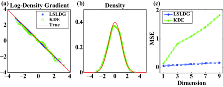
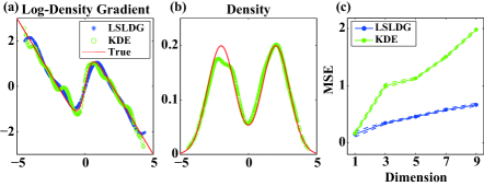
Figure 2: LSLDG vs. KDE for Gaussian data. (a) Profiles of the true log-density gradient and its estimates obtained by LSLDG and KDE. (b) True and estimated densities by KDE. (c) Averages and standard deviations of mean-squared errors to the true log-density gradients as functions of input dimensionality over $100$ runs.

Figure 3: LSLDG vs. KDE for data sampled from a mixture of two Gaussians.

In this section, we demonstrate the usefulness of the proposed LSLDG method.

5.1 Illustration of Log-Density Gradient Estimation

We first illustrate how LSLDG estimates log-density gradients using $n=1,000$ samples drawn from $p(\boldsymbol{x})$ where either

• $p(\boldsymbol{x})$ is the standard normal density, or

• $p(\boldsymbol{x})$ is a mixture of two Gaussians with means $2$ and $-2$, variances $1$ and $1$, and mixing coefficients $0.5$ and $0.5$.

As described in Section 2.3, the Gaussian width $\sigma$ and the regularization parameter $\lambda$ are chosen by 5-fold cross-validation from the following candidate set:

$$\{10^{-2},10^{-1.5},10^{-1},10^{-0.5},10^{0},10^{0.5},10^{1}\}.$$ (6)

We compare the performance of the proposed method with Gaussian KDE, where the Gaussian width is chosen by likelihood cross-validation from the same candidate set in (6).

The results for the Gaussian data are presented in Figure 3. This shows that LSLDG gives a nice smooth estimate, while the estimate by KDE is rather oscillating. Note that KDE still works well as a density estimator (see Figure 3(b)). This clearly illustrates that a good density estimate (obtained by KDE) does not necessarily yield a good estimate of the log-density gradient. We repeated this experiment $100$ times and the mean squared error to the true log-density gradient is plotted in Figure 3(c) as a function of the input dimensionality. This shows that while the error of KDE increases sharply as a function of dimensionality, that of LSLDG increases only mildly. This implies that the advantage of directly estimating the log-density gradient is more prominent in high-dimensional cases. Similar tendencies can be observed also for the Gaussian mixture data (Figure 3), where the added dimensions in Figure 3(c) simply follow the standard normal distribution.

5.2 Illustration of Clustering

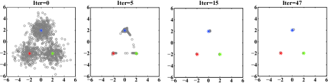
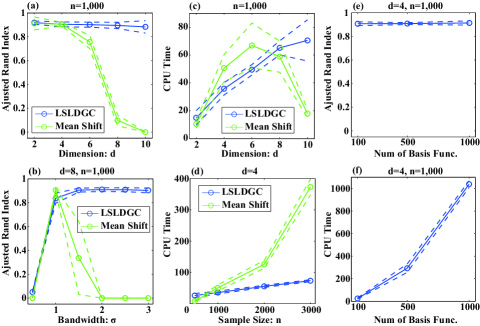
Figure 4: Transition of data points toward the modes at the initial state, $5$th, $15$th, and $47$th iterations. The blue, red, and green symbols represent the three centers of the Gaussian mixture model.

Figure 5: Means and standard deviations of clustering performance over $100$ runs measured by ARI as functions of (a) dimensionality of data and (b) the Gaussian width (when dimensionality is $8$). CPU time is also compared with respect to (c) dimensionality and (d) sample size. (e) ARI and (f) CPU time for LSLDG clustering are plotted as functions of the number of basis functions.

Next, we illustrate the behavior of LSLDG clustering on $1,000$ samples gathered from the mixture of three Gaussians whose means were $(0,2)$, $(-2,-2)$, and $(2,-2)$, and covariance matrices were the identity matrices. The mixing coefficients were $0.4$, $0.3$, and $0.3$. Figure 5 illustrates the transition of data samples over update iterations, showing that all points converge to the nearest modes within 47 iterations.

We compare the performance of the proposed method with the Gaussian mean shift [6, 7]. To investigate the effect of high dimensionality, further dimensions following the standard normal distribution are added to data points. We measure the clustering performance by the adjusted Rand index (ARI) [14], which takes the maximum value $1$ when clustering is perfect.

ARI values are plotted as a function of input dimensionality in Figure 5(a) averaged over $100$ runs. When the dimensionality of data is in the range of $2$–$4$, both methods work very well. However, when the dimensionality is beyond $4$, the performance of the Gaussian mean shift drops sharply. In contrast, for the proposed method, reasonably high ARI values are still attained even when the dimensionality is increased.

Figure 5(b) plots the ARI values for $d=8$ when the Gaussian widths are changed. This shows that the proposed LSLDG clustering performs well for a wide range of Gaussian widths, while the ARI plot for the Gaussian mean shift is peaky. This implies that selection of Gaussian widths is much harder for the Gaussian mean shift than LSLDG clustering.

LSLDG clustering is also advantageous in terms of the computational costs. Figure 5(c) shows that CPU time of LSLDG clustering is almost the same as or shorter than that of the mean shift, when the ARI values for both methods are high enough. The shorter CPU time of the mean shift when the dimensionality is more than 8 comes from the fact that a smaller bandwidth is chosen; then the number of clusters is more close to the number of kernels and thus the mean shift converges very quickly, although this performs poorly. With the same sample size, LSLDG clustering is much faster than the mean shift, as plotted in Figure 5(d). The speedup was brought by reducing the kernel centers, which was shown to significantly improve the computation costs without worsening the clustering performance, as depicted in Figures 5(e) and (f).

5.3 Image Discontinuity Preserving Smoothing and Image Segmentation

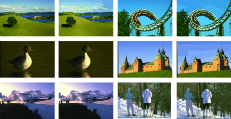
Figure 6: Examples of images after LSLDG clustering. The left-hand figure in each pair is the input image, and the right-hand one is the image after LSLDG clustering.

The mean shift has been successively applied to image discontinuity preserving smoothing and segmentation tasks [9, 25, 27]. Here, we investigate the performance of LSLDG clustering in those tasks.

As image data, we used the Berkeley segmentation dataset (BSD500) [1]. From one image, the information of color (three dimensions) and spatial positions (two dimensions) were extracted per pixel. Thus, the dimensionality of data is five, and the total number of samples is the same as the total number of pixels. As often assumed in the mean shift [9], for image data, we used the following mother basis function:

$$\phi_{i}(\boldsymbol{x}) =\exp\left(-\frac{\|\boldsymbol{x}^{c}-\boldsymbol{c}_{i}^{c}\|}{2\sigma_{c}^{2}}\right)\exp\left(-\frac{\|\boldsymbol{x}^{s}-\boldsymbol{c}_{i}^{s}\|}{2\sigma_{s}^{2}}\right),$$ (7)

$\boldsymbol{x}^{c}$ and $\boldsymbol{x}^{s}$ denote the elements for colors and spatial positions in a data vector $\boldsymbol{x}$, respectively. $\boldsymbol{c}_{i}^{c}$ and $\boldsymbol{c}_{i}^{s}$ are the Gaussian centers. For the two Gaussian width $\sigma_{c}$ and $\sigma_{s}$, cross-validation was performed as in Section 2.3. In this experiment, we used a reduced image ($11$ by $16$ or $16$ by $11$ pixels) as the Gaussian centers. For the Gaussian mean shift, (7) was employed as a Gaussian kernel, and the two Gaussian widths were cross-validated based on the likelihood.

Six examples of color images after LSLDG clustering are shown in Figure 6. In the results, some of the segments, such as grass, are cleanly smoothed out, while the edges outlining the objects are preserved. These properties are similar to the results for the mean shift [9].

Next, to clarify the difference from the mean shift, we compared the performance measured by ARI. In this experiment, the input images were reduced to $81$ by $121$ (or $121$ by $81$) pixels. Since this benchmark dataset contains several ground truths per image, we simply computed the mean ARI value to all the ground truths.

The ARI values are summarized in Table 1. LSLDG clustering shows a better ARI value on image segmentation.

Table 1: Mean ARI values for $200$ images. The numbers in the parentheses are standard deviations. The difference between the methods is statistically significant at level $1\%$ by the t-test.

Mean Shift	LSLDGC
0.08(0.03)	0.13(0.06)

5.4 Performance Comparison to Existing Clustering Methods

Finally, we compare LSLDG clustering to existing clustering methods using accelerometric sensor and speech data.

For comparison, we employed K-means (KM) [19], spectral clustering (SC) [21, 20] with the Gaussian similarity, and Gaussian mean shift. Since the user has to set the number of clusters in advance for KM and SC, we set it as the true number of clusters in each dataset. For the Gaussian mean shift, the Gaussian width was chosen by likelihood cross-validation. For LSLDG, in this experiment, we modify the linear-in-parameter model as

$$g_{j}(\boldsymbol{x})=\sum_{i=1}^{n}\theta_{i}\psi_{i,j}(\boldsymbol{x})=\boldsymbol{\theta}^{\top}\boldsymbol{\psi}_{j}(\boldsymbol{x}).$$

The main difference from the model introduced in Section 2.2 is that the coefficients $\theta_{i}$ do not depend on $j$, namely, the dimensionality of data. This modification considerably decreases the computational costs to much higher dimensional data.

In this experiment, we used the following two datasets where $d$ denotes the dimensionality of data, $n$ denotes the number of samples, and $c$ denotes the number of true clusters:

1. Accelerometry $(d=5,n=300,~{}\mathrm{and}~{}c=3)$. The ALKAN dataset, which contains $3$-axis (i.e., x-, y-, and z-axes) accelerometric data.

2. Speech $(d=50,n=400,~{}\mathrm{and}~{}c=2)$. An in-house speech dataset, which contains short utterance samples recorded from $2$ male subjects speaking in French with sampling rate $44.1$kHz.

The details of the two datasets can be seen in [23]. For each dataset, as preprocessing, the variance was normalized after centering in the element-wise manner.

The experimental results are described in Table 2. For the accelerometry dataset, LSLDG clustering shows the best performance of all the methods in the table. In addition to the superior performance, another advantage is that LSLDG clustering does not include any parameters which have to be manually tuned. On the other hand, KM and SC require the users to fix the number of clusters beforehand, which largely influences the clustering performance. Thus, LSLDG clustering would be easier to use in practice. For the speech dataset, LSLDG outperforms the existing clustering methods again (Table 2). Since the dimensionality of the dataset, $d=50$, is much higher than the accelerometry dataset ($d=5$), LSLDG seems to perform well on high dimensional data, while the mean shift does not work well on high-dimensional data, as already indicated in Section 5.2.

Table 2: Mean ARI for various methods over $100$ runs. The standard deviations are indicated in the parentheses. The best method in terms of the average ARI and methods judged to be comparable to the best one by the t-test at the significance level $1\%$ are described in boldface.

Accelerometry ($d=5,~{}n=300,~{}\mathrm{and}~{}c=3$)
KM	SC	Mean Shift	LSLDGC
0.50(0.03)	0.20(0.26)	0.51(0.05)	0.61(0.13)
Speech ($d=50,~{}n=400,~{}\mathrm{and}~{}c=2$)
KM	SC	Mean Shift	LSLDGC
0.00(0.00)	0.00(0.00)	0.00(0.00)	0.13(0.02)

6 Conclusions

In this paper, we developed a method to directly estimate the log-density gradient, and constructed a clustering algorithm on it. The proposed log-density gradient estimator can be regarded as a non-parametric extension of score matching [15, 22], and the proposed clustering algorithm can be regarded as an extension of the mean shift algorithm [7, 9, 12]. The key advantage compared to the mean shift is that the proposed clustering method works well on high-dimensional data for which the mean shift works poorly. Furthermore, we showed empirically that the proposed method outperforms existing clustering methods, even in higher-dimensional problems.

References

- [1] P. Arbelaez, M. Maire, C. Fowlkes, and J. Malik. Contour detection and hierarchical image segmentation. IEEE Transactions on Pattern Analysis and Machine Intelligence, 33(5):898–916, 2011.
- [2] A. Argyriou, T. Evgeniou, and M. Pontil. Multi-task feature learning. In NIPS, pages 41–48, Cambridge, MA, 2007. MIT Press.
- [3] A. Basu, I. R. Harris, N. L. Hjort, and M. C. Jones. Robust and efficient estimation by minimising a density power divergence. Biometrika, 85(3):549–559, 1998.
- [4] L. M. Bregman. The relaxation method of finding the common point of convex sets and its application to the solution of problems in convex programming. USSR Computational Mathematics and Mathematical Physics, 7(3):200–217, 1967.
- [5] M.Á. Carreira-Perpiñán. Fast nonparametric clustering with gaussian blurring mean-shift. In Proceedings of the 23rd international conference on Machine learning, pages 153–160. ACM, 2006.
- [6] M.Á. Carreira-Perpiñán. Gaussian mean-shift is an EM algorithm. IEEE Transactions on Pattern Analysis and Machine Intelligence, 29(5):767–776, 2007.
- [7] Y. Cheng. Mean shift, mode seeking, and clustering. IEEE Transactions on Pattern Analysis and Machine Intelligence, 17(8):790–799, 1995.
- [8] R. T. Collins. Mean-shift blob tracking through scale space. In IEEE Computer Society Conference on Computer Vision and Pattern Recognition 2003, volume 2, pages 234–240. IEEE, 2003.
- [9] D. Comaniciu and P. Meer. Mean shift: A robust approach toward feature space analysis. IEEE Transactions on Pattern Analysis and Machine Intelligence, 24(5):603–619, 2002.
- [10] D. Comaniciu, V. Ramesh, and P. Meer. Real-time tracking of non-rigid objects using mean shift. In IEEE Conference on Computer Vision and Pattern Recognition 2000, volume 2, pages 142–149. IEEE, 2000.
- [11] T. Evgeniou and M. Pontil. Regularized multi-task learning. In Proceedings of the Tenth ACM SIGKDD International Conference on Knowledge Discovery and Data Mining (KDD2004), pages 109–117. ACM, 2004.
- [12] K. Fukunaga and L. Hostetler. The estimation of the gradient of a density function, with applications in pattern recognition. IEEE Transactions on Information Theory, 21(1):32–40, 1975.
- [13] T. Hastie, S. Rosset, R. Tibshirani, and J. Zhu. The entire regularization path for the support vector machine. Journal of Machine Learning Research, 5:1391–1415, 2004.
- [14] L. Hubert and P. Arabie. Comparing partitions. Journal of Classification, 2(1):193–218, 1985.
- [15] A. Hyvärinen. Estimation of non-normalized statistical models by score matching. Journal of Machine Learning Research, 6:695–709, 2005.
- [16] A. Hyvärinen. Some extensions of score matching. Computational Statistics & Data Analysis, 51(5):2499–2512, 2007.
- [17] T. Kanamori, T. Suzuki, and M. Sugiyama. Computational complexity of kernel-based density-ratio estimation: A condition number analysis. Machine Learning, 90(3):431–460, 2013.
- [18] S. Kullback and R. A. Leibler. On information and sufficiency. The Annals of Mathematical Statistics, 22:79–86, 1951.
- [19] J. B. MacQueen. Some methods for classification and analysis of multivariate observations. In Proceedings of the 5th Berkeley Symposium on Mathematical Statistics and Probability, volume 1, pages 281–297, Berkeley, CA, USA, 1967. University of California Press.
- [20] A. Y. Ng, M. I. Jordan, and Y. Weiss. On spectral clustering: Analysis and an algorithm. In T. G. Dietterich, S. Becker, and Z. Ghahramani, editors, NIPS, pages 849–856, Cambridge, MA, USA, 2002. MIT Press.
- [21] J. Shi and J. Malik. Normalized cuts and image segmentation. IEEE Transactions on Pattern Analysis and Machine Intelligence, 22(8):888–905, 2000.
- [22] B. Sriperumbudur, K. Fukumizu, A. Gretton, and A. Hyvärinen. Density estimation in infinite dimensional exponential families. arXiv preprint arXiv:1312.3516, 2013.
- [23] M. Sugiyama, G. Niu, M. Yamada, M. Kimura, and H. Hachiya. Information-maximization clustering based on squared-loss mutual information. Neural Computation, 26(1):84–131, 2014.
- [24] M. Sugiyama, T. Suzuki, and T. Kanamori. Density ratio matching under the Bregman divergence: A unified framework of density ratio estimation. Annals of the Institute of Statistical Mathematics, 64(5):1009–1044, 2012.
- [25] W. Tao, H. Jin, and Y. Zhang. Color image segmentation based on mean shift and normalized cuts. IEEE Transactions on Systems, Man, and Cybernetics, Part B: Cybernetics, 37(5):1382–1389, 2007.
- [26] R. Tibshirani. Regression shrinkage and subset selection with the lasso. Journal of the Royal Statistical Society, Series B, 58(1):267–288, 1996.
- [27] J. Wang, B. Thiesson, Y. Xu, and M. Cohen. Image and video segmentation by anisotropic kernel mean shift. In Computer Vision-ECCV 2004, pages 238–249. Springer, 2004.