Efficient Semidefinite Branch-and-Cut for MAP-MRF Inference

Abstract

We propose a Branch-and-Cut (B&C) method for solving general MAP-MRF inference problems. The core of our method is a very efficient bounding procedure, which combines scalable semidefinite programming (SDP) and a cutting-plane method for seeking violated constraints. In order to further speed up the computation, several strategies have been exploited, including model reduction, warm start and removal of inactive constraints.

We analyze the performance of the proposed method under different settings, and demonstrate that our method either outperforms or performs on par with state-of-the-art approaches. Especially when the connectivities are dense or when the relative magnitudes of the unary costs are low, we achieve the best reported results. Experiments show that the proposed algorithm achieves better approximation than the state-of-the-art methods within a variety of time budgets on challenging non-submodular MAP-MRF inference problems.

1 Introduction

Markov Random Fields (MRFs) have been used to model a variety of problems in computer vision, including semantic image segmentation, restoration, 3D reconstruction and stereo matching, amongst a lot of others. Finding the maximum a posteriori (MAP) solution to general MRF problems is typically NP-hard, however, and many approaches have been proposed to solve such problems, approximately or exactly (see Kappes et al. (2015); Szeliski et al. (2008); Kumar et al. (2009); Kolmogorov and Rother (2006); Givry et al. (2014) for comparative studies).

Graph cuts based methods Boykov et al. (2001); Kolmogorov and Zabin (2004); Kolmogorov and Rother (2007) have been applied to a number of MAP problems in computer vision. Binary MRFs with submodular pairwise potentials can be solved exactly and efficiently by graph cuts. The QPBO Rother et al. (2007); Kolmogorov and Rother (2007) algorithm can obtain a part of the globally optimal solution for some non-submodular, binary, pairwise MRFs, but its performance degrades as the portion of non-submodular potentials increases and in the case of highly connected graphs or weak unary potentials Rother et al. (2007). For multi-label MRFs, expansion move and swap move algorithms Boykov et al. (2001) have been employed to find a strong local optimum with the property that no expansion move (swap move) can decrease the energy. However, this optimality is guaranteed only if the binary subproblem at each iteration is solved globally. In particular, the binary subproblem is typically required to be submodular to guarantee this optimality.

Another class of popular inference approaches is based on message passing. Max-product belief propagation Pearl (1988); Weiss and Freeman (2001); Sun et al. (2002); Felzenszwalb and Huttenlocher (2006) obtains exact solutions to tree-structured graphs, single-cycle graphs Aji et al. (1998); Weiss (2000), and maximum weight matching on bipartite graphs Bayati et al. (2005). For graphs with cycles, approximate solutions can also be obtained using max-product belief propagation, but there is no convergence guarantee. Tree-reweighted max-product (TRW) message-passing Wainwright et al. (2005); Kolmogorov (2006); Kolmogorov and Wainwright (2005) differs from belief propagation in that it maintains a lower-bound to the minimum energy and can be used to measure the quality of approximate solutions. TRW message passing is proved Kolmogorov and Wainwright (2005) to be exact for binary submodular MRFs. Kolmogorov Kolmogorov (2006) proposed an improved version of TRW, called TRW-S, with convergence guarantee that TRW does not have.

Many aforementioned approaches have underlying connections to the standard linear programming (LP) relaxation optimizing over local marginal polytope Shlezinger (1976); Werner (2007); Wainwright and Jordan (2008). The ordinary max-product updates Pearl (1988) can be considered as a Lagrangian approach to the dual of the standard LP relaxation, for tree-structured graphs. However, this relationship cannot be generalized to graphs with cycles. For binary pairwise graphs, QPBO and TRW message passing exactly solve the standard LP relaxation Kolmogorov and Wainwright (2005). The standard LP relaxation can achieve exact solutions for tree-structured graphs or binary graphs with submodular potentials. It is proved in Kumar et al. (2009) that the standard LP relaxation dominates second-order cone programming (SOCP) relaxation Kumar et al. (2006) and quadratic programming (QP) relaxation Ravikumar and Lafferty (2006).

Standard LP algorithms such as interior-point methods are usually computationally inefficient for large-scale MAP problems, as they do not exploit the graph structure. To this end, a number of specific approaches to solve LP relaxation for MAP problems have been proposed, such as block coordinate descent methods Kolmogorov (2006); Globerson and Jaakkola (2007), subgradient descent methods Komodakis et al. (2011); Kappes et al. (2010); Jojic et al. (2010), bundle methods Kappes et al. (2012), proximal methods Ravikumar et al. (2010), ADMM Martins et al. (2011a, b); Meshi and Globerson (2011) and smoothing methods Hazan and Shashua (2010); Johnson et al. (2007); Ravikumar et al. (2010); Savchynskyy et al. (2012).

However, it has been shown in Komodakis and Paragios (2008); Werner (2008); Sontag et al. (2008); Batra et al. (2011) that the standard LP relaxation is still not tight enough for many hard MAP problems in real applications. Especially, the above-mentioned methods usually perform poorly for the class of densely-connected graphs with weak unary potentials and a large portion of non-submodular pairwise potentials (which are of major interests in this paper). Because there are a large number of (potentially frustrated) long cycles in densely-connected graphs, the standard LP relaxation is likely to provide loose bounds. Two approaches can be adopted to alleviate this issue. The first direction is based on LP relaxation with high-order consistency constraints Sontag et al. (2008); Werner (2008); Komodakis and Paragios (2008); Johnson (2008); Batra et al. (2011); Sontag et al. (2012); and the second one is to use semidefinite programming (SDP) relaxation Torr (2003); Jordan and Wainwright (2003); Olsson et al. (2007); Schellewald and Schnörr (2005); Joulin et al. (2010); Peng et al. (2012); Wang et al. (2013); Huang et al. (2014); Frostig et al. (2014).

As the standard LP relaxation only enforces edge consistency constraints over pseudo-marginals of variables, it can be loose due to the existence of violated high-order consistency constraints. Cluster based methods Sontag et al. (2008); Komodakis and Paragios (2008); Batra et al. (2011); Sontag et al. (2012) can be used to tighten the standard LP relaxation by incrementally adding high-order consistency constraints. Methods for searching violated high-order constraints include dictionary enumeration for triplets or other short cycles Sontag et al. (2008); Batra et al. (2011) and separation algorithms for long cycles Sontag and Jaakkola (2007); Sontag et al. (2012).

SDP relaxation provides an alternative tighter bound for MAP-MRF inference problems, compared with LP relaxation. SDP is of great importance in developing approximation algorithms for some NP-hard optimization problems, and usually provides more accurate solutions. In particular for the classical maxcut problem, it achieves the best approximation ratio of $0.879$ Goemans and Williamson (1995). Primal-dual interior-point methods Alizadeh et al. (1998); Andersen et al. (2003); Nesterov and Todd (1998); Ye et al. (1994); Helmberg (1994) are considered as state-of-the-art general SDP solvers, which in the worst case require $\mathcal{O}(m^{3}+mn^{3}h^{3}+m^{2}n^{2}h^{2})$ arithmetic operations and $\mathcal{O}(m^{2}+n^{2}h^{2})$ memory requirement to solve SDP relaxation to an MAP problem with $n$ nodes, $h$ states per node and $m$ linear constraints. The exponent in the polynomial complexity bound is so great as to preclude practical applications of interior-point methods to even medium sized problems. This has significantly hampered the use of SDP relaxations in MAP-MRF inference.

Some approaches Burer and Monteiro (2003); Joulin et al. (2010); Peng et al. (2012); Frostig et al. (2014) solve SDP relaxation efficiently based on the low-rank approximation of p.s.d. matrix: $\mathbf{X}=\mathbf{Y}\mathbf{Y}^{\!\top}$ (such that p.s.d. constraints are eliminated). However, these methods need to solve a sequence of non-convex problems, and may get stuck in a local-optimal point. Multivariate weight updates based methods Arora et al. (2012, 2005); Arora and Kale (2007); Hazan (2008); Garber and Hazan (2011); Laue (2012) solve specific SDP problems inexactly, but need many iterations to converge to accurate solutions. Augmented Lagrangian methods Malick et al. (2009); Zhao et al. (2010); Wen et al. (2010); Huang et al. (2014) have also been proposed for solving SDP problems, which can be viewed as an instance of gradient descent methods Rockafellar (1973) and may have a slow convergence rate.

It is shown in Wainwright and Jordan (2008) that MAP LP relaxation with local consistency constraints and conventional SDP relaxation without considering local consistency constraints are mutually incomparable, which means that neither of them is tighter than the other. Thus combining conventional SDP relaxation and standard/high-order local consistency constraints together would produce an even tighter bound. Unfortunately, this combination results in a very challenging optimization problem, not only because of the computational inefficiency of SDP itself, but also due to the large number of linear constraints arising from standard/high-order LP relaxation.

In this paper, we propose an efficient SDP approximation/bounding approach, which is faster than state-of-the-art competing methods and able to handle a large number of linear constraints. A Branch-and-Cut (B&C) method is developed based on this SDP bounding procedure. Our approach can be used to achieve either the exact solution or an accurate approximation to general MAP-MRF inference problems with a time budget, and does so at a lower computational cost than state-of-the-art competing methods. The main contributions of this paper are as follows.

• We present an approximate inference approach based on a scalable SDP algorithm Wang et al. (2013) and cutting-plane. The proposed formulation minimizes the energy over the intersection of the semidefinite and polyhedral outer-bounds arising from SDP and standard/high-order LP relaxation respectively. Such optimization schemes result in SDP problems with a large number of linear constraints $m$. Significantly, our proposed SDP method scales linearly in $m$ (i.e., ${\cal O}(m)$)—a sharp contrast to standard interior-point methods with complexity of ${\cal O}(m^{3})$. The method proceeds by incrementally adding violated constraints until the required solution quality is achieved. Our method is much faster than interior-point methods while still maintains a comparable lower-bound of the minimum energy.

• The proposed SDP approximate/bounding method is embedded into a B&C framework for exactly solving MAP-MRF inference problems. We also introduce a few techniques to optimize the bounding and branching procedures, including model reduction, warm start and removal of inactive constraints.

• We analyze the performance on a variety of MRF graphic models, which demonstrates that our method performs better than recent competing approaches, especially when the graph connectivity is dense and/or the unary potentials are weak.

Related work We review some research work that is closely related to ours. The proposed approach is motivated by the line of our prior work in Shen et al. (2011); Wang et al. (2013). While the work in Shen et al. (2011); Wang et al. (2013) focuses on distance metric learning and image segmentation, our work here considers approximate and exact methods for general MAP-MRF inference problems.

Different B&B algorithms have been proposed for MAP-MRF inference. Sun et al. Sun et al. (2012) proposed a B&B method (refer to as MPLP-BB) based on LP relaxation. DAOOPT Otten and Dechter (2012) is another B&B method based on LP relaxation, which combines several sophisticated techniques, including And/Or search spaces, the mini-bucket approach and stochastic local search. In our experiments, MPLP-BB and DAOOPT are outperformed by our method. Peng et al. Peng et al. (2012) developed an approximate inference method for optimizing over the intersection of semidefinite bound and local marginal polytope. Note that the optimization technique in their work is different from ours. There, the p.s.d. constraint and local marginal polytope are separated using dual decomposition, and then the SDP subproblem is solved using non-convex QP, which results in a local optimum. On the contrary, our method processes the p.s.d. and linear constraints altogether and optimizes a convex problem with a guarantee of being globally optimal.

SDP-based B&B or B&C approaches have also been widely studied for integer/continuous quadratic problems. Krislock et al. Rislock et al. (2012) introduced an SDP-based branch-and-bound (B&B) method to solve Max-Cut problems. An experimental comparison was performed in Armbruster et al. (2012) between LP- and SDP-based B&B methods for graph bisection problems, which showed that SDP-based methods are better for graphs with a few thousands nodes. The algorithm in Burer and Vandenbussche (2008) solves real-valued nonconvex quadratic programs using a finite B&B algorithm in which the bound of each branch is computed by semidefinite relaxation. The work in Dinh et al. (2010) introduced an exact solver for binary quadratic programs, which combines DC (difference of convex functions) algorithms and SDP-based B&B approaches. Mars and Schewe Mars and Schewe (2012) proposed an SDP-based B&B method for mixed-integer semidefinite programs. SDP-based cutting plane algorithms were studied in Helmberg and Weismantel (1998); Helmberg et al. (2000, 1996); Helmberg and Rendl (1998); Helmberg et al. (1995) for binary quadratic programs, in which linear constraints arising from cut polytope were used to strengthen the SDP relaxation. In contrast to the above approaches, our algorithm aims to solve the MAP inference problems for discrete graphical models, and uses a number of specific speedup strategies.

Notation Table 1 lists the notation used in this paper:

$\mathbf{X}$	A matrix (bold upper-case letters).
$\mathbf{x}$	A column vector (bold lower-case letters).
$\mathbb{R}$	The set of real numbers.
$\mathcal{S}^{n}$	The set of $n\times n$ symmetric matrices.
$\mathcal{S}^{n}_{+}$	The cone of positive semidefinite (p.s.d.) $n\times n$ matrices.
$\mathbf{X}\succcurlyeq 0$	The matrix $\mathbf{X}$ is positive semidefinite.
$\leq,\geq$	Inequality between scalars or element-wise inequality between column vectors.
$\mathbf{1}(\cdot)$	Indicator function, $1$ if the statement is true and $0$ otherwise.
$\mathrm{trace}(\cdot)$	Trace of a matrix.
$\mathrm{rank}(\cdot)$	Rank of a matrix.
$\mathrm{diag}(\mathbf{X})$	The main diagonal vector of the matrix $\mathbf{X}$.
$\mathrm{diag}(\mathbf{x})$	A diagonal matrix consisting of the input vector $\mathbf{x}$ as diagonal elements.
$\lVert\cdot\rVert_{1}$, $\lVert\cdot\rVert_{2}$	$\ell_{1}$ and $\ell_{2}$ norm of a vector.
$\lVert\cdot\rVert_{F}$	Frobenius-norm of a matrix.
$\langle\cdot,\cdot\rangle$	Inner product of two matrices.
$\nabla\mathrm{f}(\cdot)$	The first-order derivatives of function $\mathrm{f}(\cdot)$.
$\lfloor x\rfloor$	The nearest integer less than or equal to $x$.

Table 1: Notation.

The remaining of this paper is organized as follows. We first introduce the basic concepts of LP and SDP relaxation to MAP problems in Section 2. Then our main contributions, the overall branch-and-cut method for energy minimization and the SDP bounding approach with cutting-plane are discussed in Sections 3 and 4 respectively. The performance of our algorithms is evaluated experimentally in Section 5.

2 LP and SDP Relaxation to MAP-MRF Inference Problems

Suppose that an MAP-MRF inference model is characterized by an undirected graph $\mathcal{G}=(\mathcal{V},\mathcal{E})$, where $\mathcal{V}$ represents the set of $n$ nodes (which is reused to represent the set of node indexes$\{1,2,\dots,n\}$) and $\mathcal{E}$ represents the set of edges. In this paper, we only consider unary and pairwise potentials, and so MAP-MRF inference problems can be expressed as the following energy minimization problem:

$$\min_{\mathbf{x}\in\mathcal{Z}^{n}}\mathrm{E}(\mathbf{x}):=\sum_{p\in\mathcal{V}}\mathrm{\theta}_{p}(x_{p})+\sum_{p<q,(p,q)\in\mathcal{E}}\mathrm{\theta}_{p,q}(x_{p},x_{q}),$$ (1)

where $\mathrm{\theta}_{p}(x_{p})$ and $\mathrm{\theta}_{p,q}(x_{p},x_{q})$ represent the unary and pairwise potentials respectively. $\mathcal{Z}=\{1,2,\dots,h\}$ refers to the set of $h$ possible states. Without loss of generality, we assume that all nodes have the same number of possible states.

It is well known that the energy minimization problem (1) is equivalent to the following LP problem:

$$\min_{\{\mathbf{y},\mathbf{Y}\}\in\mathcal{M}(\mathcal{G},\mathcal{Z})}\mathrm{E}(\mathbf{y},\mathbf{Y}) :=\sum_{p\in\mathcal{V},i\in\mathcal{Z}}\theta_{p}(i)y_{p,i}\,\,+$$ (2)

$$\sum_{p<q,(p,q)\in\mathcal{E},i,j\in\mathcal{Z}}\theta_{p,q}(i,j)Y_{pi,qj}$$

where the set $\mathcal{M}(\mathcal{G,\mathcal{Z}})$ refers to the marginal polytope with respect to graph $\mathcal{G}$ and the state space $\mathcal{Z}$:

$$\mathcal{M}(\mathcal{G},\mathcal{Z}):=$$ (3)

$$\,\,\left\{\mathbf{y},\mathbf{Y}\ \begin{array}[]{|lll}&\exists\,\mathrm{Pr}(\mathbf{x}),\,\mathrm{s.t.}&\\ &y_{p,i}\!=\!\mathrm{Pr}(x_{p}\!=\!i),&\forall p\!\in\!\mathcal{V},i\!\in\!\mathcal{Z},\\ &Y_{pi,qj}\!=\!\mathrm{Pr}(x_{p}\!=\!i,x_{q}\!=\!j),&\forall(p,q)\!\in\!\mathcal{E},i\!\in\!\mathcal{Z}.\!\end{array}\right\}$$ (7)

In the above definition, $\{y_{p,i}\}_{i\in\mathcal{Z}}$ and $\{Y_{pi,qj}\}_{i,j\in\mathcal{Z}}$ refer to singleton and pairwise pseudomarginals with respect to each node $p\!\in\!\mathcal{V}$ and each edge $(p,q)\!\in\!\mathcal{E}$ respectively, which are globally realizable by some joint distribution $\mathrm{Pr}()$ over $\mathbf{x}\in\mathcal{Z}^{n}$. Each vertex (extreme point) of $\mathcal{M}(\mathcal{G},\mathcal{Z})$ is integer ($\{0,1\}$-valued) and corresponds to a valid assignment $\mathbf{x}\in\mathcal{Z}^{n}$. So there is always a binary optimal solution to the LP problem (2).

Although the above LP problem only contains $\mathcal{O}(|\mathcal{E}|+|\mathcal{V}|)$ number of variables, it generally requires exponential number of linear constraints to describe $\mathcal{M}(\mathcal{G},\mathcal{Z})$. To address this difficulty, the standard LP relaxation Shlezinger (1976); Werner (2007); Wainwright and Jordan (2008) optimizes the objective function of (2) over a tractable set, called local marginal polytope:

$$\mathcal{M}_{L}(\mathcal{G},\mathcal{Z})\!:=\!$$ (8)

$$\,\,\left\{\mathbf{y},\mathbf{Y}\ \begin{array}[]{|lll}&\ \mathbf{y}\geq\mathbf{0};\ \mathbf{Y}\geq\mathbf{0};&\\ &\ {\sum_{i\in\mathcal{Z}}}y_{p,i}\!=\!1,&\forall p\!\in\!\mathcal{V};\\ &\ {\sum_{j\in\mathcal{Z}}}Y_{pi,qj}\!=\!y_{p,i},&\forall(p,q)\!\in\!\mathcal{E},i\!\in\!\mathcal{Z}.\end{array}\right\},$$ (12)

which is a convex polyhedral outer-bound on $\mathcal{M}(\mathcal{G},\mathcal{Z})$. That is, $\mathcal{M}(\mathcal{G},\mathcal{Z})\subseteq\mathcal{M}_{L}(\mathcal{G},\mathcal{Z})$. Its number of linear constraints grows linearly with respect to the graph size but quadratically with the size of $\mathcal{Z}$. It is known (see Wainwright and Jordan (2008) for example) that any vertex of $\mathcal{M}(\mathcal{G},\mathcal{Z})$ is also a vertex of $\mathcal{M}_{L}(\mathcal{G},\mathcal{Z})$, and for a graph $\mathcal{G}$ with cycles, $\mathcal{M}_{L}(\mathcal{G},\mathcal{Z})$ also contains fractional vertexes lying outside $\mathcal{M}(\mathcal{G},\mathcal{Z})$. Consequently, we have the following important property of the standard LP relaxation (see Wainwright and Jordan (2008)):

Theorem 2.1

(Optimality guarantee of LP relaxation)

If the solution to the LP relaxation: $\displaystyle{\min_{\{\mathbf{y},\mathbf{Y}\}\in\mathcal{M}_{L}(\mathcal{G},\mathcal{Z})}}\mathrm{E}(\mathbf{y},\mathbf{Y})$ is integer, it is the exact MAP solution.

The edge consistency is preserved in $\mathcal{M}_{L}(\mathcal{G},\mathcal{Z})$, but high-order consistency is not enforced. Cluster based methods Sontag et al. (2008); Batra et al. (2011); Sontag et al. (2012) iteratively add to LP relaxation high-order consistency constraints, and provide incrementally improved lower-bounds to the minimal energy: $\min_{\mathbf{x}\in\mathcal{Z}^{n}}\mathrm{E}(\mathbf{x})$.

Alternatively, SDP relaxation provides a different convex outer-bound on $\mathcal{M}(\mathcal{G},\mathcal{Z})$. Consider a symmetric matrix consisting of $\mathbf{y}$ and $\mathbf{Y}$:

$$\Omega(\mathbf{y},\mathbf{Y})\!:=\!\left[{\begin{smallmatrix}1&y_{1,1}&\cdots&y_{p,i}&\cdots&y_{q,j}&\cdots&y_{n,h}\\ y_{1,1}&Y_{11,11}&\cdots&Y_{11,pi}&\cdots&Y_{11,qj}&\cdots&Y_{11,nh}\\ \raisebox{3.0pt}{$\scalebox{0.75}{\vdots}$}&\raisebox{3.0pt}{$\scalebox{0.75}{\vdots}$}&&\raisebox{3.0pt}{$\scalebox{0.75}{\vdots}$}&&\raisebox{3.0pt}{$\scalebox{0.75}{\vdots}$}&&\raisebox{3.0pt}{$\scalebox{0.75}{\vdots}$}\\ y_{pi}&Y_{pi,11}&\cdots&Y_{pi,pi}&\cdots&Y_{pi,qj}&\cdots&Y_{pi,nh}\\ \raisebox{3.0pt}{$\scalebox{0.75}{\vdots}$}&\raisebox{3.0pt}{$\scalebox{0.75}{\vdots}$}&&\raisebox{3.0pt}{$\scalebox{0.75}{\vdots}$}&&\raisebox{3.0pt}{$\scalebox{0.75}{\vdots}$}&&\raisebox{3.0pt}{$\scalebox{0.75}{\vdots}$}\\ y_{qj}&Y_{qj,11}&\cdots&Y_{qj,pi}&\cdots&Y_{qj,qj}&\cdots&Y_{qj,nh}\\ \raisebox{3.0pt}{$\scalebox{0.75}{\vdots}$}&\raisebox{3.0pt}{$\scalebox{0.75}{\vdots}$}&&\raisebox{3.0pt}{$\scalebox{0.75}{\vdots}$}&&\raisebox{3.0pt}{$\scalebox{0.75}{\vdots}$}&&\raisebox{3.0pt}{$\scalebox{0.75}{\vdots}$}\\ y_{nh}&Y_{nh,11}&\cdots&Y_{nh,pi}&\cdots&Y_{nh,qj}&\cdots&Y_{nh,nh}\end{smallmatrix}}\right],$$ (13)

where $Y_{pi,qj}:=y_{p,i}\!\cdot\!y_{q,j},\forall(p,q)\!\notin\!\mathcal{E},i,j\!\in\!\mathcal{Z}$. At any vertex of $\mathcal{M}(\mathcal{G},\mathcal{Z})$, $\Omega(\mathbf{y},\mathbf{Y})=\Omega(\mathbf{y},\mathbf{y}\mathbf{y}^{\!\top})=\left[\begin{smallmatrix}1,\hfill&\mathbf{y}^{\!\top}\hfill\\ \mathbf{y},\hfill&\mathbf{y}\mathbf{y}^{\!\top}\end{smallmatrix}\right]$ $\succcurlyeq\mathbf{0}$ is a rank-$1$ positive semidefinite matrix.

By discarding the non-convex rank-$1$ constraint, we obtain the following convex outer-bound on $\mathcal{M}(\mathcal{G},\mathcal{Z})$:

$$\mathcal{P}(\mathcal{G}):=\{\mathbf{y},\mathbf{Y}\lvert\Omega(\mathbf{y},\mathbf{Y})\succcurlyeq\mathbf{0}\},$$ (14)

which generally contains curved boundaries. It is shown in Wainwright and Jordan (2008) that local marginal polytope $\mathcal{M}_{L}(\mathcal{G},\mathcal{Z})$ and the semidefinite outer-bound $\mathcal{P}(\mathcal{G})$ are mutually incomparable, which means that neither of them dominates the other. We attempt to combine the local marginal polytope and semidefinite outer-bound in this work such that a tighter bound can be achieved. To solve the resulted SDP problem, which may have a large number of constraints, scalable SDP solvers are developed.

In general, both LP and SDP relaxation do not provide feasible integer solutions to the original non-submodular energy minimization problem. Thus a rounding procedure is needed to transform a fractional solution given by LP/SDP relaxation to a feasible integer solution. A simple rounding procedure for both LP/SDP relaxation is to round each variable independently based on the singleton pseudo-marginals $\mathbf{y}$:

$$x_{p}=\arg\max_{i\in\mathcal{Z}}y_{p,i},\,\,p=1,2,\cdots,n.$$ (15)

Better rounding methods would consider the labelling over all variables jointly, which can be done by considering the reparameterized objective Kolmogorov (2006) or pairwise pseudo-marginals $\mathbf{Y}$ conditioned by already labelled variables. For max-cut problems, the random hyperplane rounding approach Goemans and Williamson (1995) for SDP relaxation delivers a bounded expected objective value. In this paper, the simple rounding procedure (15) is adopted for our SDP solver, followed by a post-processing procedure based on ICM Besag (1986) (see Section 4.5).

3 Branch-and-Cut for Energy Minimization

In this section, the overall algorithm of B&C for the energy minimization problem (1) is given in Algorithm 1 and then the subproblem selection and branching strategies are presented.

3.1 The Branch-and-Bound Method

First, we briefly revisit B&B methods Horst et al. (2000); Hendrix et al. (2010). As a method for global optimization of nonconvex problems, B&B methods rely on two procedures which compute upper- and lower-bounds on the global optimum. Considering a minimization problem, the upper-bound can be obtained by choosing any point in the feasible set. A local search method is usually performed to improve the upper-bound. On the other hand, the lower-bound can be computed from a convex relaxation to the original non-convex problem.

At each iteration of B&B (Algorithm 1), a subproblem is selected from the priority queue $\mathcal{Q}$ (Step $1$) and its upper-/lower-bounds are computed (Step $2$). In Step $3$, the global upper-bound ($\mathrm{gub}$) is updated in each iteration as the minimum of the upper-bounds over all branches, while the global lower-bound ($\mathrm{glb}$) is updated as the minimum of the lower-bounds over all leaf branches. All subproblems with a lower-bound not smaller than the global upper-bound are pruned in Step $4$. If the selected subproblem cannot be pruned, its feasible set $\mathcal{D}$ is separated into at least two convex sets (Step $5$). B&B algorithms terminate when the global upper-bound and lower-bound are sufficiently close to each other.

There are several essential components in B&B: bounding ($\mathrm{bound}(\mathcal{D})$), subproblem selection ($\mathrm{pop}(\mathcal{Q})$) and branching ($\mathrm{split}(\mathcal{D},\mathbf{y})$). The bounds computed by the bounding procedure are assumed to become tighter as the feasible set shrink. Especially when the size of a feasible set shrinks to a point, the difference between upper and low er bounds needs to converge to zero. It is shown in Proposition 1 that our SDP bounding approach satisfies these assumptions. A comprehensive study of branching and subproblem selection strategies can be found in Achterberg et al. (2005); Land and Powell (1979); Linderoth and Savelsbergh (1999); Mitra (1973), in which a number of sophisticated rules are investigated. In this work, we adopt simple rules for branching and subproblem selection and rely on the tight bounding procedure to improve the performance.

Input: the original energy minimization problem $\min_{\mathbf{x}\in\mathcal{Z}^{n}}\mathrm{E}(\mathbf{x})$.

Initialization: global upper-/lower-bounds $\mathrm{gub}=+\infty$, $\mathrm{glb}=-\infty$; priority queue $\mathcal{Q}=\{\mathcal{Z}^{n}\}$.

while $\mathcal{Q}\neq\emptyset$ do

       Step 1 Subproblem Selection: $\mathcal{D}=\mathrm{pop}(\mathcal{Q})$.

      Step 2 Bounding:
- $[\mathrm{ub},\mathrm{lb},\mathbf{x},\mathbf{y}]=\mbox{bound}(\mathcal{D})$ (see Algorithm. 3);

      Step 3 Update global bounds:
- $\mathrm{glb}=\min(\mathrm{lb},\min_{\mathcal{D}^{\prime}\in\mathcal{Q}}\mathrm{lb}(\mathcal{D}^{\prime}))$;
- if $\mathrm{gub}>\mathrm{ub}$ then $\mathrm{gub}=\mathrm{ub}$, $\mathbf{x}^{\star}=\mathbf{x}$.;

      

      Step 4 Pruning: $\mathcal{Q}\leftarrow\mathcal{Q}\backslash\{\mathcal{D}^{\prime}|\mathcal{D}^{\prime}\in\mathcal{Q},\mathrm{lb}(\mathcal{D}^{\prime})\geq\mathrm{gub}\}$.

      Step 5 Branching:
if $\mathrm{lb}<\mathrm{gub}$ then

             - $[\mathcal{D}_{1},\mathcal{D}_{2}]=\mathrm{split}(\mathcal{D},\mathbf{y})$ (see Algorithm 2);
- $\mathcal{Q}\leftarrow\{\mathcal{Q},\mathcal{D}_{1},\mathcal{D}_{2}\}$.

      

Output: $\mathbf{x}^{\star}$.

Algorithm 1 Semidefinite Branch-and-Cut (SDBC)

Input: The search space $\mathcal{D}:=\mathcal{Z}^{\mathcal{D}}_{1}\times\mathcal{Z}^{\mathcal{D}}_{2}\times\dots\times\mathcal{Z}^{\mathcal{D}}_{|\mathcal{V}|}$, and the singleton pseudomarginals $\{y_{p,i}\}_{i\in\mathcal{Z}^{\mathcal{D}}_{p}},\forall p\in\mathcal{V}$.

Step 1 Node selection: $\varphi=\arg\displaystyle{\min_{p\in\mathcal{V},|\mathcal{Z}^{\mathcal{D}}_{p}|>1}}(\max_{i\in\mathcal{Z}^{\mathcal{D}}_{p}}y_{p,i})$.

Step 2 State ordering: obtain the state order $i_{1},i_{2},\dots,i_{|\mathcal{Z}^{\mathcal{D}}_{\varphi}|}$ such that $y_{\varphi,i_{1}}\geq y_{\varphi,i_{2}}\geq\dots\geq y_{\varphi,i_{|\mathcal{Z}^{\mathcal{D}}_{\varphi}|}}$.

Step 3 Branching: separate $\mathcal{Z}^{\mathcal{D}}_{\varphi}$ into two disjointed subsets $\mathcal{Z}^{\mathcal{D}}_{\varphi,1}=\{i_{1},\dots,i_{\lfloor{|\mathcal{Z}^{\mathcal{D}}_{\varphi}|}/{2}\rfloor}\}$ and $\mathcal{Z}^{\mathcal{D}}_{\varphi,2}=\{i_{\lfloor{|\mathcal{Z}^{\mathcal{D}}_{\varphi}|}/{2}\rfloor+1},\dots i_{|\mathcal{Z}^{\mathcal{D}}_{\varphi}|}\}$.

Output: $\mathcal{D}_{1}\!=\!\mathcal{Z}^{\mathcal{D}}_{1}\times\dots\times\mathcal{Z}^{\mathcal{D}}_{\varphi,1}\times\dots\times\mathcal{Z}^{\mathcal{D}}_{|\mathcal{V}|}$ and $\mathcal{D}_{2}\!=\!\mathcal{Z}^{\mathcal{D}}_{1}\times\dots\times\mathcal{Z}^{\mathcal{D}}_{\varphi,2}\times\dots\times\mathcal{Z}^{\mathcal{D}}_{|\mathcal{V}|}$.

Algorithm 2 The branching procedure, $[\mathcal{D}_{1},\mathcal{D}_{2}]=\mathrm{split}(\mathcal{D},\mathbf{y})$.

3.2 Subproblem Selection: $\mathcal{D}=\mathrm{pop}(\mathcal{Q})$

All unresolved subproblems (represented by their respective feasible sets) are stored in the priority queue $\mathcal{Q}$. At each iteration of B&B, the subproblem with the highest priority will be selected and split. In our implementation, subproblems are sorted according to the quality of their lower-bounds, and the subproblem with the worst lower-bound will be split firstly. In other words,

$$\mathcal{D}=\mathrm{pop}(\mathcal{Q})=\arg\min_{\mathcal{D}^{\prime}\in\mathcal{Q}}\mathrm{lb}(\mathcal{D}^{\prime}),$$ (16)

where $\mathcal{D}:=\mathcal{Z}^{\mathcal{D}}_{1}\times\mathcal{Z}^{\mathcal{D}}_{2}\times\dots\times\mathcal{Z}^{\mathcal{D}}_{|\mathcal{V}|}$ and $\mathcal{Z}^{\mathcal{D}}_{p}$ denotes the set of possible states for each node $p\in\mathcal{V}$ within the feasible set $\mathcal{D}$. Note that a subset of elements of $\mathbf{y}$ are enforced to be $0$s or $1$s in the subproblem with respect to $\mathcal{D}$:

$$y_{p,i}=0, \quad\mbox{if }i\in\{\mathcal{Z}\backslash\mathcal{Z}^{\mathcal{D}}_{p}\},\forall p\in\mathcal{V},$$ (17a)

$$y_{p,i}=1, \quad\mbox{if }i\in\mathcal{Z}^{\mathcal{D}}_{p}\mbox{ and }|\mathcal{Z}^{\mathcal{D}}_{p}|=1,\forall p\in\mathcal{V}.$$ (17b)

3.3 Branching: $[\mathcal{D}_{1},\mathcal{D}_{2}]=\mathrm{split}(\mathcal{D},\mathbf{y})$

At the branching step, the input feasible set $\mathcal{D}$ is further split into two disjointed sets $\mathcal{D}_{1}$ and $\mathcal{D}_{2}$, by selecting a node and split its state space in halves.

Node Selection We employ the “difficult first” strategy, which selects the node that is the most difficult to discretize. Remind that $\{y_{p,i}\}_{i\in\mathcal{Z}^{\mathcal{D}}_{p}}$ can be considered as a singleton pseudo-marginal for each node $p\in\mathcal{V}$, if it resides in the local marginal polytope (8). If this distribution does not concentrate on a single point (in other words, spreads evenly over all states), then the corresponding node is considered to be difficult to discretize. Accordingly, a simple strategy is adopted for node selection in this work:

$$\varphi=\arg\displaystyle{\min_{p\in\mathcal{V},|\mathcal{Z}^{\mathcal{D}}_{p}|>1}}(\max_{i\in\mathcal{Z}^{\mathcal{D}}_{p}}y_{p,i}).$$ (18)

States Ordering As in Sun et al. (2012), the possible states of the selected node $\varphi$, i.e. $i_{1},i_{2},\dots,i_{|\mathcal{Z}^{\mathcal{D}}_{\varphi}|}$, are ordered dynamically in each iteration of branching, such that $y_{\varphi,i_{1}}\geq y_{\varphi,i_{2}}\geq\dots\geq y_{\varphi,i_{|\mathcal{Z}^{\mathcal{D}}_{\varphi}|}}$. Then the most and the least probable states are separated into two sets: $\mathcal{Z}^{\mathcal{D}}_{\varphi,1}=\{i_{1},\dots,i_{\lfloor{|\mathcal{Z}^{\mathcal{D}}_{\varphi}|}/{2}\rfloor}\}$ and $\mathcal{Z}^{\mathcal{D}}_{\varphi,2}=\{i_{\lfloor{|\mathcal{Z}^{\mathcal{D}}_{\varphi}|}/{2}\rfloor+1},\dots i_{|\mathcal{Z}^{\mathcal{D}}_{\varphi}|}\}$.

Now the last component in the B&C approach (Algorithm 1) to be studied is the bounding procedure, $\mathrm{bound}(\mathcal{D})$, which we discuss in the following section.

4 An Efficient SDP Bounding Procedure with Cutting-plane

In this section, we consider the following SDP relaxation to the original energy minimization problem (1):

$$\min_{\mathbf{y},\mathbf{Y}}\,\, \mathrm{E}(\mathbf{y},\mathbf{Y})$$ (19a)

$$\mathrm{s.t.}\,\, \eqref{eq:sdprelax_cons1},\eqref{eq:sdprelax_cons2},\eqref{eq:sdprelax_cons3},\eqref{eq:sdprelax_cons4},\eqref{eq:sdprelax_cons5},\eqref{eq:tricons},\eqref{eq:cyccons},\eqref{eq:owccons},$$ (19b)

$$\Omega(\mathbf{y},\mathbf{Y})\succcurlyeq\mathbf{0},$$ (19c)

where (19b) corresponds to the additional linear constraints to be discussed in Section 4.1. The above formulation can be easily extended to any subproblem $\mathcal{D}$ in Algorithm 1, by reparameterization or enforcing additional constraints (17). A main observation is that the linear constraints arising from standard/high-order LP relaxation can be used to significantly tighten the following naive SDP relaxation: However, the resulted large-scale SDP optimization problem, which in particular has a large number of linear constraints, render standard interior-point SDP solvers inapplicable. A scalable SDP solver combined with cutting-plane is proposed to solve such SDP optimization in Section 4.2 and 4.3. Then the complexity of our method is discussed in Section 4.4 and several speeding-up strategies are proposed in Section 4.5.

4.1 Linear Constraints that Tighten the Semidefinite Outer-Bound

Besides the p.s.d. constraint, several classes of linear constraints arising from LP relaxation can be added to SDP relaxation to tighten the bound.

$\mathbf{0/1}$-Integer Constraints These constraints arise from the integer constraints $y_{p,i}\!\in\!\{0,1\}$, which is equivalent to $y_{p,i}\!=\!y_{p,i}^{2}$, for each node $p\in\mathcal{V}$ and state $i\in\mathcal{Z}$:

$$Y_{pi,pi}=y_{p,i},\,\,\forall p\in\mathcal{V},i\in\mathcal{Z}.$$ (20)

There are $nh$ such constraints for a graph with $n$ nodes and $h$ states per node.

Local Normalization Constraints Because only one state $i\in\mathcal{Z}$ can be assigned to each node $p\in\mathcal{V}$, we have:

$$\textstyle{\sum_{i\in\mathcal{Z}}}y_{p,i}=1.\,\,\forall p\in\mathcal{V},$$ (21)

There are $n$ local normalization constraints in total. Note that for any $\{\mathbf{y},\mathbf{Y}\}\in\mathcal{P}(\mathcal{G})\cap\eqref{eq:sdprelax_cons1}\cap\eqref{eq:sdprelax_cons2}$, if $\mathrm{rank}(\Omega(\mathbf{y},\mathbf{Y}))=1$, then $\{\mathbf{y},\mathbf{Y}\}$ is a vertex of $\mathcal{M}(\mathcal{G},\mathcal{Z})$.

Non-Negativity Constraints Deriving from $Y_{pi,qi}=y_{p,i}\cdot y_{q,j}$ and $\mathbf{y}\in\{0,1\}^{nh}$, the following constraints holds:

$$Y_{pi,qj}\geq 0,\,\,\forall(p,q)\in\mathcal{E},i,j\in\mathcal{Z}.$$ (22)

There are $\lvert\mathcal{E}\rvert h^{2}$ such constraints for a graph with $\lvert\mathcal{E}\rvert$ edges. The number becomes $n(n-1)h^{2}/2$ for a fully-connected graph. Huang et al. Huang et al. (2014) have shown that without the non-negativity constraints, SDP relaxation is loose for submodular functions.

Edge Marginalization Constraints For each edge $(p,q)\in\mathcal{E}$ and $i\in\mathcal{Z}$, we have $\sum_{j\in\mathcal{Z}}Y_{pi,qj}=y_{pi}\cdot\sum_{j\in\mathcal{Z}}y_{qj}$. Therefore the following constraints can be derived:

$$\!{\textstyle\sum_{j\in\mathcal{Z}}Y_{pi,qj}=y_{p,i},\,\,\forall(p,q)\in\mathcal{E},i\in\mathcal{Z}.}$$ (23)

There are in total $2\lvert\mathcal{E}\rvert h$ such constraints ($n(n-1)h$ for fully-connected graphs). Note that local normalization (21), non-negativity (22) and marginalization (23) constraints force $\{\mathbf{y},\mathbf{Y}\}$ to lie in local marginal polytope $\mathcal{M}_{L}(\mathcal{G},\mathcal{Z})$.

Gangster Operators Because $Y_{pi,pj}=y_{p,i}\cdot y_{p,j}$ and each node $p\in\mathcal{V}$ can only be assigned with one state $i\in\mathcal{Z}$, at least one of $y_{p,i}$ and $y_{p,j}$ should be zero. Then we have the following constraints:

$$Y_{pi,pj}=0,\,\,\forall p\in\mathcal{V},\forall i\neq j,i,j\in\mathcal{Z}.$$ (24)

These constraints are referred to as gangster operators, as they shoot holes (zeros) in $\mathbf{Y}$. Considering matrix symmetry, there are $nh(h-1)/2$ such constraints in total. Schellewald and Schnorr Schellewald and Schnörr (2005) have used these constraints for SDP approaches to subgraph matching.

Note that the above linear constraints are directly defined on the marginal polytope. In this work, we also consider the following a few classes of linear constraints defined on the cut polytope or equivalently binary marginal polytope, which can be extended to $\mathcal{M}(\mathcal{G},\mathcal{Z})$ by projecting a non-binary graph to a binary graph. Comprehensive studies of linear constraints for cut polytope or binary marginal polytope can be found in Barahona and Mahjoub (1986); Deza et al. (1992); Chopra and Rao (1993) and the references therein.

Triangular Inequalities Considering three binary variables $\pi_{p}$, $\pi_{q}$, $\pi_{r}$ and define $\delta_{p,q}:=\mathbf{1}[\pi_{p}\neq\pi_{q}]$, then we have:

$$\delta_{p,q}+\delta_{q,r}+\delta_{p,r}\leq 2,$$ (25a)

$$\delta_{p,q}-\delta_{q,r}-\delta_{p,r}\leq 0,$$ (25b)

$$-\delta_{p,q}+\delta_{q,r}-\delta_{p,r}\leq 0,$$ (25c)

$$-\delta_{p,q}-\delta_{q,r}+\delta_{p,r}\leq 0,$$ (25d)

which are facet defining for a cut polytope Barahona and Mahjoub (1986). The number of triangular inequalities is cubic in the number of binary variables.

Cycle Inequalities They arise from the fact that there must be an even number of edge-cuts for any cycle of variables. For a cycle $C$ and any $F\subseteq C$ such that $|F|$ is odd, the inequality can be expressed as:

$$\sum_{(p,q)\in C\backslash F}\delta_{p,q}+\sum_{(p,q)\in F}(1-\delta_{p,q})\geq 1.$$ (26)

The triangular inequalities (25b) (25c), (25d) can be considered as special cases of cycle inequalities. A cycle inequality is facet defining for a cut polytope if and only if the cycle is chordless Barahona and Mahjoub (1986). There are an exponential number of cycle inequalities in a graph. However, the most violated one can be found in $\mathcal{O}(n^{3}h^{3})$ time for a dense graph using the separation procedure shown in Barahona and Mahjoub (1986); Deza and Laurent (1997).

Odd-wheel Inequalities Consider a cycle $C$ of length $s=2t+3$, where the integer $t\geq 0$. $V(C)$ denotes the node set of $C$ and $\pi_{r}$ refers to a center node not in $V(C)$. Then the following inequality

$$\sum_{(p,q)\in C}\delta_{p,q}-\sum_{p\in V(C)}\delta_{p,r}\leq\frac{|C|-1}{2},$$ (27)

is called ‘$s$-wheel inequality’ or simply ‘odd-wheel inequality’. This class of constraints is not facet-defining for a cut polytope, but it is facet defining for a multicut polytope Deza et al. (1992); Chopra and Rao (1993). There are also an exponential number of the above constraints with respect to the number of binary variables. For a solution satisfying all cycle inequalities, the separation procedure shown in Deza and Laurent (1997) can find the most violated odd-wheel inequality using $\mathcal{O}(n^{4}h^{4})$ time for a dense graph.

We adopt the method proposed in Sontag and Jaakkola (2007); Sontag et al. (2012) for projecting non-binary graphs to binary graphs. Firstly, $\pi_{p}^{s}$ is defined as a binary variable separating the state space of node $p$ into two disjoint non-empty sets $\mathcal{Z}_{s}$ and $\mathcal{Z}\!\setminus\!\mathcal{Z}_{s}$, that is $\pi_{p}^{s}=1$, if $x_{p}\in\mathcal{Z}_{s}$, and $0$ otherwise. $\pi_{p}=\{\pi_{p}^{1},\pi_{p}^{2},\dots\}$ represents a collection of partitions with respect to node $p$. Then the non-binary graph $\mathcal{G}=(\mathcal{V},\mathcal{E})$ can be projected to a binary graph $\mathcal{G}_{\pi}=(\mathcal{V}_{\pi},\mathcal{E}_{\pi})$, where

$$\mathcal{V}_{\pi} =\{\pi_{p}^{s}\mid p\in\mathcal{V},s\leq|\pi_{p}|\},$$ (28a)

$$\mathcal{E}_{\pi} =\{(\pi_{q}^{s},\pi_{p}^{t})\mid(p,q)\in\mathcal{E},s\leq|\pi_{p}|,t\leq|\pi_{q}|\}.$$ (28b)

Note that $\delta_{\pi_{q}^{s},\pi_{p}^{t}}:=\mathbf{1}[\pi_{p}^{s}\neq\pi_{q}^{t}]$ can be expressed in terms of $\mathbf{Y}$ in (13), that is $\delta_{\pi_{q}^{s},\pi_{p}^{t}}=\sum_{\{i\in\mathcal{Z}_{s},j\notin\mathcal{Z}_{t}\}\cap\{i\notin\mathcal{Z}_{s},j\in\mathcal{Z}_{t}\}}Y_{pi,qj}$. In this paper, we define $\mathcal{Z}_{s}=\{s\},\forall s=1,2,\cdots,h$, such that each $h$-state variable $x_{p}$ is projected to $h$ binary variables.

Note that the projected inequalities are not necessarily facet-defining for the non-binary graph, although some of them are facet-defining on the projected binary graph.

Input: The energy minimization problem $\min_{\mathbf{x}\in\mathcal{D}}\mathrm{E}(\mathbf{x})$, where $\mathcal{D}$ is a subset of the space of potential label assignment $\mathcal{Z}^{n}$; $\Psi$ is the working set of constraints. $\Psi_{\mathrm{addi}}$ is the pool of additional constraints (22), (23), (25), (26) and (27) to be added in cutting-plane. Parameters $\gamma\!>\!0$, $\delta\!>\!1$; Maximum iterations $K_{\mathrm{init}}$, $K_{\mathrm{inner}}$ and $K_{\mathrm{outer}}$. The initial set of constraints $\psi_{\mathrm{init}}$ and the corresponding dual variable $\mathbf{u}_{\mathrm{init}}$.

Step 1 Initial Bounding:
- Model reduction (Optional): $\mathcal{D}\leftarrow\mathrm{QPBO}(\mathcal{D})$;
- Initialize the working set and dual variable: $\Psi\leftarrow\psi_{\mathrm{init}}$, $\mathbf{u}\leftarrow\mathbf{u}_{\mathrm{init}}$.
- Construct the dual problem (29) with respect to $\mathcal{D}$, $\Psi$ and $\gamma$.
for $k=1,2,\dots,K_{\mathrm{init}}$ do

       - Dual variable update: $\mathbf{u}\leftarrow\mathbf{u}+\rho\mathbf{H}\nabla\mathrm{d}_{\gamma}(\mathbf{u})$.
- Lower-bound update: $\mathrm{lb}\leftarrow\mathrm{d}_{\gamma}(\mathbf{u})$.
- Goto Step 3 if any stop condition is met (see Section 4.5).

- Compute the primal variable: $\Omega(\mathbf{y},\mathbf{Y})=\gamma\Pi_{\mathcal{S}^{n\!h\!+\!1}_{+}}(\mathbf{C}(\mathbf{u}))$.

Step 2 Cutting-Plane:
for $k_{1}=1,2,\dots,K_{\mathrm{outer}}$ do

       - $\psi_{\mathrm{in}}\leftarrow$ inactive constraints selected from $\Psi$.
- $\psi_{\mathrm{vi}}\leftarrow$ constraints violated by $\Omega(\mathbf{y},\mathbf{Y})$ selected from $\Psi_{\mathrm{addi}}$.
- $\Psi\leftarrow\{\Psi\backslash\psi_{\mathrm{in}}\}\cup\psi_{\mathrm{vi}}$. $\gamma\leftarrow\delta\cdot\gamma$.
- Construct the dual problem (29). with respect to $\mathcal{D}$, $\Psi$ and $\gamma$.
- Update the dual variable: $\mathbf{u}\leftarrow\{\mathbf{u},\mathbf{0}\}$, where $\mathbf{0}$ corresponds to the dual variables with respect to $\psi$.
for $k_{2}=1,2,\dots,K_{\mathrm{inner}}$ do

             - Dual variable update: $\mathbf{u}\leftarrow\mathbf{u}+\rho\mathbf{H}\nabla\mathrm{d}_{\gamma}(\mathbf{u})$.
- Lower-bound update: $\mathrm{lb}\leftarrow\mathrm{d}_{\gamma}(\mathbf{u})$.

       - Goto Step 3 if any stop condition is met.
- Compute the primal variable: $\Omega(\mathbf{y},\mathbf{Y})=\gamma\Pi_{\mathcal{S}^{n\!h\!+\!1}_{+}}(\mathbf{C}(\mathbf{u}))$.

Step 3 Rounding:
- Generate a discrete solution $\mathbf{x}$ by rounding $\mathbf{y}$ (see Equation (15)).
- Improve $\mathbf{x}$ using RICM (see Section 4.5).
- $\mathrm{ub}\leftarrow\mathrm{E}(\mathbf{x})$.

Output: $\mathrm{ub}$, $\mathrm{lb}$, $\mathbf{x}$ and $\mathbf{y}$.

Algorithm 3 SDP Bounding Procedure ($[\mathrm{ub},\mathrm{lb},\mathbf{x},\mathbf{y}]=\mathrm{bound}(\mathcal{D})$)

4.2 Initial Bounding Using SDCut

The feasible set of the SDP relaxation (19) is the intersection of semidefinite outer-bound $\mathcal{P}(\mathcal{G})$ and the polyhedral outer-bound produced by standard/high-order LP relaxation. There are several difficulties in optimizing the SDP problem (19). First of all, it is computationally inefficient to solve SDP problems using classic interior-point methods, which has the computational complexity of $\mathcal{O}(m^{3}+mn^{3}h^{3}+m^{2}n^{2}h^{2})$ and memory requirement of $\mathcal{O}(m^{2}+n^{2}h^{2})$, where $m$ is the number of linear constraints. Secondly, the linear constraints involved in (19) are very complex. It requires $\mathcal{O}(n^{2}h^{2})$ constraints to describe the local marginal polytope for a fully-connected graph, which makes the computational complexity of interior-point methods increase to $\mathcal{O}(n^{6}h^{6})$. The total number of cycle inequalities grows even exponentially with the graph size. To this end, we propose to adapt the SDCut method proposed in our prior work Wang et al. (2013) to optimize (19) and use cutting-plane to cope with the large number of linear constraints.

In the following, $\mathbf{A},\mathbf{B}_{i}\in\mathcal{S}^{nh+1},i=1,2,\cdots,m$, $\mathbf{b}\in\mathbb{R}^{m}$ are defined such that $\langle\Omega(\mathbf{y},\mathbf{Y}),\mathbf{A}\rangle=\mathrm{E}(\mathbf{y},\mathbf{Y})$ and linear constraints in (19b) are also expressed in the form of matrix inner-products: $\langle\Omega(\mathbf{y},\mathbf{Y}),\mathbf{B}_{i}\rangle=b_{i},\,\forall i\in\mathcal{I}_{eq}$, $\langle\Omega(\mathbf{y},\mathbf{Y}),\mathbf{B}_{i}\rangle\leq b_{i},\,\forall i\in\mathcal{I}_{in}$, where $\mathcal{I}_{eq}$, $\mathcal{I}_{in}$ refer to non-overlapping indexes for linear equality and inequality constraints respectively. $m\!=\!|\mathcal{I}_{eq}|+|\mathcal{I}_{in}|$.

SDCut Wang et al. (2013) is proposed to approximately solve a subclass of SDP problems in which the trace of p.s.d. matrix variables is fixed. Instead of minimizing the linear objective function $\langle\Omega(\mathbf{y},\mathbf{Y}),\mathbf{A}\rangle$, SDCut minimizes the perturbed function $\langle\Omega(\mathbf{y},\mathbf{Y}),\mathbf{A}\rangle+\frac{1}{2\gamma}(\lVert\Omega(\mathbf{y},\mathbf{Y})\rVert^{2}_{F}-\eta^{2})$ over the constraints shown in (19b), where $\eta:=\mathrm{trace}(\Omega(\mathbf{y},\mathbf{Y}))=n\!+\!1$ ($\eta$ can be discarded since it is a constant) in our case and $\gamma>0$. It is shown in Wang et al. (2013) that with an appropriate $\gamma$, the solution of the perturbed problem is “close” to that of the original SDP problem.

Furthermore, by introducing the perturbed objective, the Lagrangian dual of SDCut can be simplified to:

$$\max_{\mathbf{u}\in\mathbb{R}^{m}}\,\, \mathrm{d}_{\gamma}(\mathbf{u})\!:=\!-\frac{\gamma}{2}\lVert\Pi_{\mathcal{S}^{n\!h\!+\!1}_{+}}(\mathbf{C}(\mathbf{u}))\rVert_{F}^{2}\!-\!\mathbf{u}^{{\!\top}}\mathbf{b}\!-\!\frac{\eta^{2}}{2\gamma},$$ (29a)

$$\mathrm{s.t.}\,\, u_{i}\geq 0,i\in\mathcal{I}_{in},$$ (29b)

where $\mathbf{C}(\mathbf{u})\!=\!-\mathbf{A}-\sum_{i=1}^{m}u_{i}\mathbf{B}_{i}$. The matrix-valued function $\Pi_{\mathcal{S}^{n\!h\!+\!1}_{+}}$ is defined as

$$\Pi_{\mathcal{S}^{n\!h\!+\!1}_{+}}(\mathbf{X}):=\mathbf{P}\mathrm{diag}(\max(0,\mathbf{\boldsymbol{\lambda}}))\mathbf{P}^{\!\top},$$

and $\mathbf{X}=\mathbf{P}\mathrm{diag}({\boldsymbol{\lambda}})\mathbf{P}^{\!\top}$ is the eigen-decomposition of the matrix $\mathbf{X}\in\mathcal{S}^{n}$, where ${\boldsymbol{\lambda}}$ denotes the vector of eigenvalues and $\mathbf{P}$ contains the corresponding (column) eigenvectors. Note that there is no p.s.d. constraint in (29) any more. Based on K.K.T. conditions, we have

$$\Omega(\mathbf{y}^{\star}_{\gamma},\mathbf{Y}^{\star}_{\gamma})=\gamma\Pi_{\mathcal{S}^{n\!h\!+\!1}_{+}}(\mathbf{C}(\mathbf{u}_{\gamma}^{\star})),$$ (30)

where $\mathbf{y}_{\gamma}^{\star}$,$\mathbf{Y}_{\gamma}^{\star}$ and $\mathbf{u}_{\gamma}^{\star}$ are the optimal solutions to the corresponding primal and dual problems with respect to $\gamma$ respectively.

We demonstrate in Appendix 7.1 that the dual formulation of SDCut (29) is actually equivalent to a penalty approach to the Lagrangian dual of the original SDP relaxation (19). For an sufficiently large parameter $\gamma$, the simplified dual (29) can be arbitrarily close to the original SDP relaxation (19), which however results in numerical problems. In many cases, it is sufficient to restrict $\gamma$ to a large value and obtain an approximate solution. Note that how to choose the value of $\gamma$ in practice to make a good tradeoff between bound quality and convergence speed is still an open question. A potential strategy is to adjust $\gamma$ adaptively at each iteration of descent step.

The dual objective function $\mathrm{d}_{\gamma}(\cdot)$ is continuously differentiable but not necessarily twice differentiable, and its gradient is given by

$$\nabla\mathrm{d}_{\gamma}(\mathbf{u})=-\gamma\Phi\left[\Pi_{\mathcal{S}^{n\!h\!+\!1}_{+}}\left(\mathbf{C}(\mathbf{u})\right)\right]-\mathbf{b},$$ (31)

where $\Phi:\mathcal{S}^{nh+1}\rightarrow\mathbb{R}^{m}$ refers to the linear transformation $\Phi[\Omega]:=[\langle\mathbf{B}_{1},\Omega\rangle,\cdots,\langle\mathbf{B}_{m},\Omega\rangle]^{\!\top}$. Consequently, we can solve the dual (29) using quasi-Newton algorithms as they only require first-order derivatives during optimization. At each descent step, quasi-Newton methods update the dual variable $\mathbf{u}$ as follows:

$$\mathbf{u}\leftarrow\mathbf{u}+\rho\mathbf{H}\nabla\mathrm{d}_{\gamma}(\mathbf{u}),$$ (32)

where $\mathbf{H}$ is the approximated inverse of Hessian matrix updated by successive gradient vectors and $1\geq\rho\geq 0$ is the step size decided by line-search.

Another important property of the simplified dual problem (29) is that for any feasible dual variable $\mathbf{u}$, the dual objective function value $\mathrm{d}_{\gamma}(\mathbf{u})$ is a lower-bound to the minimum energy ${\min_{\mathbf{x}\in\mathcal{Z}^{n}}}\mathrm{E}(\mathbf{x})$ Wang et al. (2013). This is beneficial for accelarating the B&B methods: the bounding procedure can be stopped once the computed lower-bound is not lower than the current global upper-bound, and the corresponding subproblem can be pruned.

In the sequel, $\mathrm{d}^{\star}_{\gamma}(\mathcal{D})$ is defined as the optimal value of the dual problem (29) constructed with respect to $\gamma$ and $\mathcal{D}\subseteq\mathcal{Z}^{n}$. In this paper, we further prove the following results for the tightness of the lower-bound yielded by $\mathrm{d}^{\star}_{\gamma}(\mathcal{D})$ (see Appendix 7.2):

Proposition 1

The following results hold: ($i$) $\forall\gamma\!>\!0,\forall\mathcal{D}_{1}\!\subseteq\!\mathcal{D}_{2}\!\subseteq\!\mathcal{Z}^{n}$, we have $\mathrm{d}^{\star}_{\gamma}(\mathcal{D}_{1})\geq\mathrm{d}^{\star}_{\gamma}(\mathcal{D}_{2})$; ($ii$) $\forall\gamma\!>\!0,\forall\mathcal{D}\!\subseteq\!\mathcal{Z}^{n}$ with $\lvert{\mathcal{D}}\rvert=1$, we have $\mathrm{d}^{\star}_{\gamma}(\mathcal{D})=\min_{\mathbf{x}\in\mathcal{D}}\mathrm{E}(\mathbf{x})$.

The first result shows that the lower-bound is improved as the search space $\mathcal{D}$ shrinks, and the second means that the gap between the lower- and upper-bound $\mathrm{E}(\mathbf{x})_{\mathbf{x}\in\mathcal{D}}-\mathrm{d}^{\star}_{\gamma}(\mathcal{D})$ converges to zero when the search space $\mathcal{D}$ shrinks to a point (namely $\lvert\mathcal{D}\rvert=1$). In particular, if $|\mathcal{D}|=1$ and only contains the MAP solution, $\arg\min_{\mathbf{x}\in\mathcal{Z}^{n}}\mathrm{E}(\mathbf{x})$, $\mathrm{d}^{\star}_{\gamma}(\mathcal{D})$ equals to the global minimum energy. These two properties are crucial when embedding the proposed bounding method into branch-and-bound.

Proposition 2

(Optimality Guarantee of SDP Relaxation) For any $\gamma>0$, suppose $\{\mathbf{y}_{\gamma}^{\star},\mathbf{Y}_{\gamma}^{\star}\}$ and $\mathbf{u}_{\gamma}^{\star}$ are the optimal/dual primal variable obtained by (30). If the rank of $(\Omega({\mathbf{y}_{\gamma}^{\star},\mathbf{Y}_{\gamma}^{\star}}))$ is $1$, then $\{\mathbf{y}_{\gamma}^{\star}$, $\mathbf{Y}_{\gamma}^{\star}\}$ yields the exact MAP solution and $\mathrm{d}_{\gamma}(\mathbf{u}_{\gamma}^{\star})$ is the minimum energy value.

The above optimality guarantee of SDP relaxation can be considered as a counterpart to Theorem 2.1 for the standard LP relaxation. Both LP and SDP relaxations drop non-convex constraints and result in a simple convex relaxation: the integer constraint is relaxed by LP relaxation and SDP relaxation drops the rank-$1$ constraint. Note that Proposition 2 can be generalized to SDP relaxation with linear constraints (20), (21).

Computationally SDCut is significantly more scalable and efficient than general interior-point methods. It is employed here to solve the SDP relaxation with linear constraints in (39c). However, there are $\mathcal{O}(n^{2}h^{2})$ number of constraints (22), (23) and the exponential number of constraints (25), (26), (27). Adding these constraints directly to SDCut is still impractical. To this end, we proposed to find and add most violated constraints via cutting-plane, which is discussed in the next section.

4.3 Cutting-Plane: Searching and Adding Violated Constraints

In practice, we find that most of the constraints (22), (23), (25), (26) and (27) are redundant after the initial bounding procedure shown in Section 4.2, which means that most of them are already satisfied after imposing the p.s.d. constraints and the linear constraints (20), (21) and (24). Therefore, cutting-plane methods can be adopted to search violated constraints in (22), (23), (25), (26) and (27), and add them to SDP relaxation at each iteration. Adding these primal constraints is equivalent to adding new variables to the dual problem (29).

Violated non-negativity (22), edge marginalization (23) constraints and triangular inequalities (25) are found by enumeration. Most violated cycle inequalities (26) are found using the separation procedure Deza and Laurent (1997). When there is no violated cycle inequality (up to certain precision), violated odd-wheel inequalities (27) are searched and added using the separation procedure shown in Deza and Laurent (1997).

The procedure of the proposed SDP bounding procedure, including initial bounding (Section 4.2) and cutting-plane (Section 4.3) are summarized in Algorithm 3. At each iteration of cutting-plane, the dual problem (29) is constructed based on three inputs: the search space $\mathcal{D}$ (for reparameterization), linear constraints set $\Psi$ and the penalty parameter $\gamma$.

4.4 Computational Complexity

L-BFGS-B Zhu et al. (1997) is used as the implementation of quasi-Newton algorithms for SDCut. At each iteration, L-BFGS-B itself requires only $\mathcal{O}(m)$ arithmetic operations and memory requirement, so SDCut scales linearly in the number of constraints $m$. The main computational burden of SDCut is the eigen-decomposition at each gradient-descent step to compute the dual objective function (29a) and its gradient (31). The eigen-solver used in this paper is the DSYEVR routine in LAPACK (an implementation of Relatively Robust Representations), which has the computational complexity of $\mathcal{O}(n^{3}h^{3})$ and the memory requirement of $\mathcal{O}(n^{2}h^{2})$.

Finding the most violated non-negativity constraint (22) and edge marginalization constraint (23) requires $\mathcal{O}(n^{2}h^{2})$ arithmetic operations, while finding violated cycle inequality needs $\mathcal{O}(n^{3}h^{3})$ arithmetic operations. To save time, only a few center node $\pi_{r}$ (see Equation (27)) is considered for odd-wheel inequalities in each cutting-plane iteration.

Therefore the overall computational complexity of the proposed SDP method is $\mathcal{O}(n^{3}h^{3})$ at each descent iteration ($m$ is less than $\mathcal{O}(n^{3}h^{3})$, so it is omitted), and the corresponding memory requirement is $\mathcal{O}(n^{2}h^{2})$. This result demonstrates that our approach is much more efficient than the classic interior-point methods, which needs $\mathcal{O}(n^{6}h^{6})$ arithmetic operations.

4.5 Strategies to Speed Up

Although the proposed SDP approximation method already provides a tight lower-bound efficiently, we proposed a few techniques to further speed up the bounding procedure of B&B.

Pre-Processing (Model Reduction) Several methods have been proposed to identify persistency for binary models Rother et al. (2007), Potts models Kovtun (2011); Swoboda et al. (2013) and general multi-label models Kohli et al. (2008); Kovtun (2011); Windheuser et al. (2012); Swoboda et al. (2014); Shekhovtsov (2014); Shekhovtsov et al. (2015). Persistencies refer to states of variables which are proved to be non-optimal or belong to at least one optimal solution. Previous work has employed persistency to reduce the model size before applying approximate Alahari et al. (2008) and exact Kappes et al. (2013a) solvers. For binary models, all variables assigned as integers by QPBO Rother et al. (2007) are persistent.

Without affecting the property of global convergence of B&B, QPBO is performed in each bounding procedure, and then the SDP bounding procedure is applied on the reduced model. In general, the computation time of QPBO is negligible compared to that of the SDP procedure. Because the size of the resulted SDP is smaller, the total computational time is reduced as well. Note that this partial optimality also holds for TRW message passing and other methods equivalent to the standard LP relaxation for binary graphs. We choose QPBO here for its fast computation.

Stop Conditions As discussed in Section 4.2, the objective value of (29), calculated at each descent step, can be cast as a lower-bound to the minimum energy. For faster computation, the bounding process is stopped before convergence if any of the following conditions is met (see Algorithm 3):

1. The lower-bound $\mathrm{lb}$ is already greater than the global upper-bound $\mathrm{gub}$, and thus this subproblem is pruned.

2. The improvement of the lower-bound $\mathrm{lb}$ between consecutive steps is smaller than the specified tolerance.

Warm Start Another strategy used in the bounding procedure to speed up the computation is “warm start”, which is performed in two levels: between different iterations of cutting-planes and bounding procedures.

1. In an iteration of cutting-plane, the dual variables are initialized by the results of the previous iteration. For the new constraints, the corresponding dual variables are filled with zeros.

2. The final working set of active constraints and the corresponding dual variables of the first bounding iteration are used to initialize those of subsequent bounding iterations ($\psi_{\mathrm{init}}$ and $\mathbf{u}_{\mathrm{init}}$ in Algorithm 3), which speed up the convergence speed of L-BFGS-B. The initial working set $\psi_{\mathrm{init}}$ of the first bounding iteration is set to contain constraints (20),(21) and (24), and $\mathbf{u}_{\mathrm{init}}$ is set to zeros.

Removing Inactive Constraints One disadvantage of cutting plane is that the size of the subproblems (the number of primal linear constraints, and correspondingly the number of dual variables) keeps increasing from iteration to iteration,

Since traditionally new constraints are added in each round but are never removed. The strategy of pruning inactive constraints has been employed to address this issue Topkis (1982); Joachims et al. (2009); Horst and Tuy (2013) in cutting-plane methods. In this work, we use a simple rule to decide which constraint should be dropped from the working set: those corresponding to zero dual variables and not violated by the current primal solution. Note that those constraints discarded by the current iteration may be re-activated in subsequent cutting-plane iterations.

Post-Processing (Stochastic Local Search)

When the dual optimization is terminated, an approximate solution $\mathbf{x}_{\text{appx}}\in\mathcal{Z}^{n}$ is calculated by rounding and an upper-bound $\mathrm{E}(\mathbf{x}_{\text{appx}})$ to the minimum energy $\min_{\mathbf{x}\in\mathcal{Z}^{n}}\mathrm{E}(\mathbf{x})$ is obtained. Local (greedy) search methods can be applied to further tighten the upper-bound. What we use here is ‘repeated iterated conditional modes’ (refer to as RICM):

1. Run Iterated Conditional Modes (ICM) Besag (1986) with $\mathbf{x}_{\text{appx}}$ as the initial point to find a local optimal solution $\mathbf{x}_{\text{local}}$. Compute the upper-bound $\mathrm{E}(\mathbf{x}_{\text{local}})$.

2. Randomly flip a portion (around $5\%$) of assignments in the initial solution $\mathbf{x}_{\text{appx}}$.

3. Repeat the steps 1 and 2 several times and select the local optimal solution $\mathbf{x}_{\text{local}}$ with the lowest upper-bound as the new approximate solution.

Note that ICM can be considered as a greedy coordinate descent method. The solution quality is guaranteed to be improved or at least not worse than the initial point. Furthermore, as ICM depends highly on the initialization, we repeat ICM several times to overcome this problem.

5 Experiments

The proposed method is evaluated in two forms: one with cutting-planes (refer to as SDBC) and one without (refer to as SDBB). Both of the SDP bounding methods in SDBB and SDBC solve the SDP relaxation (19) approximately based on the simplified dual formulation (29). The only difference is that SDBC imposes all linear constraints listed in (19b), while SDBB only considers constraints (20), (21) and (24). The following algorithms for MAP-MRF inference are compared against ours.

1) As a baseline, the lower-bound produced by TRWS Kolmogorov (2006) is compared with SDBC.

2) Sontag et al. Sontag et al. (2008, 2012) proposed to tighten the LP relaxation to MAP problems by incrementally introducing cluster consistency constraints, for example, triplet clusters Sontag et al. (2008) (refer to as MPLP-CP-v1) or long cycles Sontag et al. (2012) (refer to as MPLP-CP-v2). The code is obtained from the author’s website. At each round, $50$ additional triplets are added to MPLP-CP-v1 and $50\!\sim\!200$ triplets plus $50\!\sim\!200$ cycles are added to MPLP-CP-v2. MPLP-CP-v1 and MPLP-CP-v2 provide lower-bounds to the global optimal energy value, which can be used to validate the exactness of a solution. For SDP relaxation methods, we compared our method with SDPT3, which represents one of the state-of-the-art implementations of interior-point methods.

3) Our method are also compared with methods based on graph cuts Kolmogorov and Rother (2007); Gorelick et al. (2014) for binary non-submodular pairwise energies. QPBO Kolmogorov and Rother (2007) can be used to exactly solve problems with a small fraction of non-submodular terms. We also use QPBO to reduce the model before applying other methods. Local submodular approximation (LSA) Gorelick et al. (2014) iteratively approximates non-submodular energies non-linearly based on trust region (refer to as LSA-TR) or auxiliary function principles.

4) Several B&B methods for energy minimization are also evaluated. Sun et al. Sun et al. (2012) proposed a B&B method (refer to as MPLP-BB) using MPLP to upper-bound the MAP value at each branch. The dual variables of MPLP at each branch are fixed, and a data structure, called range maximum query, is pre-constructed to speed up the bound calculation significantly. The parameters of MPLP-BB are set to the default values, except that the number of initial MPLP iterations is set to $1000$.

DAOOPT Otten and Dechter (2012) implements the And/Or Branch and Bound paradigm, which also uses mini-bucket heuristic for pruning search space and limited discrepancy search (LDS) to find an initial solution quickly. It achieves the best performance in the PIC2011 Challenge Elidan and Globerson (2011). In this paper, the memory limit of DAOOPT is set to $8$GB and the discrepancy limit of LDS is set to $2$. The commercial integer linear program solver, IBM CPLEX IBM (2015) (denoted by ILP), is also evaluated in the experiments. Some specialized algorithms Kernighan and Lin (1970); Bonato et al. (2014); Kappes et al. (2011, 2013b) are also investigated for some particular data sets.

To perform a fair comparison, all the implementations of compared methods are obtained from the author’s website or from the OpenGM2 toolbox Andres et al. (2014) and tested on one core of a $2.7$GHz Intel CPU with $4$GB free memory, except for DAOOPT ($10$GB) and ILP ($40$GB). Note that some experimental results of competitive methods are obtained from Andres et al. (2014), which is evaluated on a faster Intel CPU ($3.2$GHz). All the methods are performed with the same procedures of pre-processing (model reduction by QPBO) and post-processing (stochastic local research by ICM). The primary results (Table 3, 4, 5 and 6) are shown in a format similar to Kappes et al. (2015), which demonstrates the upper-bound (energy value of the final integer solution) and lower-bound (to the optimal energy value), averaged over all instances of each problem. For an algorithm, the number of instances for which it achieves the best upper-/lower-bound among all algorithms (denoted as $\#$Best-ub and $\#$Best-lb respectively) and the number of instances to which it gives the exact solution (denoted as $\#$Exact) are also demonstrated for better comparison. As in Kappes et al. (2015), a solution is considered to be exact if the difference between the lower-bound and upper-bound is less than $10^{-5}$ in terms of absolute value or less than $10^{-8}$ in terms of relative value.

The implementation of our algorithm is written in matlab and the implementation of other methods are mainly implemented in C/C++. We would expect a further improvement in the speed of our method if it were implemented in optimized C/C++.

5.1 Performance Analysis

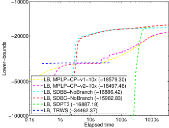
Figure 1: Lower-bounds given by different algorithms on the model “deer$\_$rescaled$\_$0034.K15.F100” ($60$ variables, $15$ states per variable) in PIC2011. SDBC is performed without branching (SDBC-NoBranch) or without both branching and cutting-plane (SDBB-NoBranch). The lower-bounds provided by LP-based methods (TRWS and MPLP-CP) are worse than SDP-based methods (SDPT3 and SDBC). SDBB-NoBranch produces a lower-bound very close to the interior-point method SDPT3. For SDBC itself, the additional constraints added through cutting-plane gives a $5\%$ increase in lower-bound.

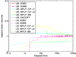
(a) fully connected, $\omega=0.4$

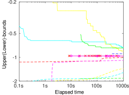
(b) fully connected, $\omega=0.2$

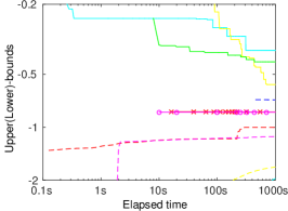
(c) fully connected, $\omega=0.1$

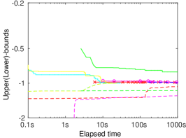
(d) $\kappa=6.56$, $\omega=0.25$

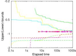
(e) $\kappa=17.06$, $\omega=0.25$

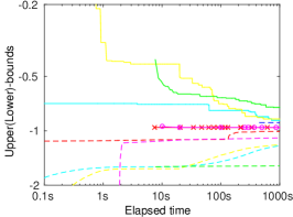
(f) $\kappa=59.06$, $\omega=0.25$

Figure 2: Upper-/lower-bound versus running time on the synthetic MAP-MRF inference problems. All the undirected graph models in this experiment have $64$ nodes and $10$ states per node, and the energy functions are randomly generated. The upper/lower bound is normalized by dividing them by the best lower-bound computed within $20$ minutes. In (a)-(c), the unary strength decreases from $0.4$ to $0.1$. When the unary strength parameter $\omega$ is large (for example, $\omega\!=\!0.4$), all methods obtain near optimal upper-bounds ($<\!-0.90$) and the superiority of SDBC is not significant. SDBC does perform significantly better than others for smaller unary strengths (for example, $\omega\!=\!0.1$). In (d)-(f), the connectivity $\kappa$ changes from $6.56$ to $59.06$. For sparse graphs (for example, $\kappa\!=\!6.56$), MPLP-CP-v1 and MPLP-CP-v2 converge quickly to the optimal and performs better than SDBC. However for dense graph models (for example, $\kappa\!=\!59.06$), SDBC yields better upper and lower bounds.

Relaxation Tightness The SDP bounding procedure embedded in SDBC is compared with state-of-the-art SDP/LP relaxation methods. SDPT3 Tütüncü et al. (2003), an implementation of interior point methods, is used to accurately solve the SDP relaxation with linear constraints (20), (21) and (24). Note that the other classes of tightening constraints are difficult to be imposed with SDPT3, due to the poor scalability of interior-point methods in the number of linear constraints. MPLP-CP-v1 and MPLP-CP-v2 tighten the standard LP relaxation (over local marginal polytope $\mathcal{M}_{L}(\mathcal{G},\mathcal{Z})$) by incrementally adding high-order consistency constraints.

In Fig. 1, the performance of these relaxation methods are compared on the lower-bounds achieved on a model in the PIC2011, “deer$\_$rescaled$\_$0034.K15.F100”, which is a fully-connected graph with $60$ nodes and $15$ states per node. In this experiment, SDBC is performed without branching, which means there is only one bounding procedure. Furthermore, to show the effectiveness of cutting-plane, SDBC is performed in two forms: with (SDBC-NoBranch) or without cutting-plane (SDBB-NoBranch).

From the results in Fig. 1, we can see that:

1. SDBB-NoBranch achieves a final lower-bound very similar to that produced by SDPT3 (the difference is only $0.1\%$), but is significantly faster than SDPT3. Note that SDBB-NoBranch and SDPT3 solve the same SDP problem, but approximately and exactly respectively. As more linear constraints are imposed, SDBC-NoBranch achieves better lower-bound than SDBB-NoBranch and SDPT3 (over $3\%$).

2. Both SDBB-NoBranch and SDBC-NoBranch yield a tighter lower-bound than TRWS, MPLP-CP-v1 and MPLP-CP-v2, which shows that the p.s.d. constraint is indeed effective.

3. Lower bounds of SDBC-NoBranch and SDBB-NoBranch converge after certain iterations. To further improve lower bounds, we need to embed the SDP bounding procedure into B&C.

Connectivity and Unary Strength We now compare the performance of SDBC, SDBB and other MAP-MRF inference methods when applied to a range of synthetic problems generated with varying parameters. We consider two factors which affect the difficulty of MAP-MRF inference problems: connectivity (i.e., the average number of neighbours per node) and unary potential strength (compared to pairwise potentials). Higher connectivity and smaller unary potential strength increase the difficulty of MAP-MRF inference problems, and degrade the performance of some existing algorithms (for example, QPBO and belief propagation Kim and Lee (2011)).

In this experiment, all the synthetic MRF models have $64$ variables and $10$ states per variable. The pairwise energies are sampled from the Gaussian distribution $\theta_{pq}(i,j)\!\thicksim\!\mathcal{N}(0,1)$, and the unary energies are sampled from $\theta_{p}(i)\!\thicksim\!\mathcal{N}(0,\omega^{2})$, where the parameter $\omega$ controls the unary strength: small $\omega$ corresponds to weak unary strength, and vice versa. $\kappa$ refers to the connectivity of a graph, which is the average number of linked neighbours per node.

The results are shown in Fig. 2, in which the curve of lower-bounds is the concatenation of two parts: the lower-bounds at the gradient-descent steps within the first bounding iteration and the lower-bounds for the subsequent bounding iterations. In the first bounding iteration of SDBB, multiple rounding procedures are conducted at $10$, $20$ and $100$ seconds respectively.

In Fig. 2 (a)-(c), fully-connected graphs ($\kappa=63$) are generated and the parameter $\omega$ is set to $\{0.4,0.2,0.1\}$ respectively. SDBC and SDBB achieve the best upper/lower bounds in most cases. Meanwhile, SDBC yields better lower-bound than that of SDBB.

The performance of all methods becomes worse when the parameter $\omega$ decreases. However, the detrimental impact on SDBC is the smallest amongst all the evaluated algorithms. The upper-bound of SDBC drops from $0.993$ ($\omega=0.4$) to $0.820$ ($\omega=0.1$), while the upper-bound of the second best method decreases from $0.975$ to $0.700$. The difference on the lower-bounds is more significant: at $\omega=0.4$, the gap between SDBC and the second best on the lower-bound is only $0.087$; while the gap increases to $0.89$ for $\omega=0.1$.

In Fig. 2 (d)-(e), $\omega$ is fixed to $0.25$ and the connectivity $\kappa$ is set to $\{6.56,17.06,59.06\}$ respectively. SDBC and SDBB perform slightly worse than MPLP-CP-v1 and MPLP-CP-v2 in terms of both upper and lower bounds when $\kappa=6.56$. For denser graphs ($\kappa\in\{17.06,59.06\}$), however, SDBC produces the best lower-/upper-bounds amongst all competing methods. We also compare SDBC and MPLP-CP-v1 on a larger sparse model from Liu et al. (2015), which contains $768$ variables, $8$ states per variable and $2252$ edges. The upper-/lower-bounds of MPLP-CP-v1 converge quickly to the global optimal solution ($-565.23$) using $0.8$ second, as it can benefit from the sparse graph structure. While SDBC scales poorer than MPLP-CP-v1 on this type of sparse models: it obtains a non-global-optimal solution ($-567.92$) using around $2$-hour runtime. Note that the focus of the proposed SDP approaches is on the dense problems with non-submodular terms and/or weak unary terms (See Wang et al. (2015) for the efforts to improve the scalability of SDP algorithms for MAP inference).

Based on the experiments on this synthetic data, we may conclude that SDBC and SDBB perform better than state-of-the-art for MRFs with high connectivity or weak unary potentials.

5.2 Image Denoising and Deconvolution

The binary submodular MRF model for image denoising is generated using the UGM code. As the energy provided by the graph-cut algorithm for such MRF models is the exact MAP value, it is used to compare with ours to validate whether the proposed B&C method converges to the exact MAP solution. As shown in Fig. 3, the result of SDBC is indeed the same as that of the graph-cut algorithm.

(a) Ground Truth

(b) Input

(c) Graph-cut

(d) SDBC

Figure 3: Image denoising. This experiment is used to validate whether SDBC converges to the globally optimal solution. The $16\!\times\!16$ input image (b) is generated by adding random Gaussian noise to all pixels of the ground truth image (a). The constructed graph model has one node per pixel and contains only unary and submodular pairwise potentials. Without branching, SDBC converges to the exact solution, which means the relative gap between the lower- and upper-bound is smaller than $10^{-8}$. The assignment by SDBC (d) is consistent with that of the graph-cut algorithm (c). The latter is well known to provide the exact MAP solution for such binary submodular MRFs.

Algorithm	Upper-bound	Lower-bound	$\#$Best-ub	$\#$Best-lb	$\#$Exact	Runtime
Runtime $\leq 20$min
SDBC	$\mathbf{-504.03}$	$\mathbf{-505.03}$	$\mathbf{6}$	$\mathbf{4}$	$0$	$1187.83$
MPLP-CP-v2	$-502.34$	$-514.48$	$2$	$2$	$\mathbf{2}$	$822.46$
ILP	$-502.88$	$-568.20$	$1$	$0$	$0$	$1220.62$
LSA-TR (euc.)	$-503.87$	$-\infty$	$0$	$0$	$0$	$1200.40$
LSA-TR (ham.)	$-503.76$	$-\infty$	$0$	$0$	$0$	$1200.10$
QPBO	$-501.92$	$-\infty$	$0$	$0$	$0$	$\mathbf{0.76}$
Runtime $\leq 1$hr
SDBC	$\mathbf{-504.08}$	$\mathbf{-504.45}$	$\mathbf{6}$	$\mathbf{4}$	$0$	$3460.10$
MPLP-CP-v2	$-503.60$	$-508.40$	$2$	$2$	$\mathbf{2}$	$\mathbf{2415.58}$
ILP	$-502.91$	$-566.41$	$2$	$0$	$0$	$3626.06$
Runtime $\leq 24$hr
SDBC	$\mathbf{-504.09}$	$\mathbf{-504.09}$	$\mathbf{6}$	$\mathbf{6}$	$\mathbf{5}$	$\mathbf{41830.36}$
MPLP-CP-v2	$-503.95$	$-505.37$	$4$	$2$	$2$	$57616.95$
ILP	$-504.07$	$-560.11$	$4$	$0$	$0$	$86026.42$

Table 2: Image deconvolution ($6$ instances, $1219$ variables and $2$ labels for each instance). LSA-TR achieves the second best average energy value within the runtime limit of $20$ minutes. MPLP-CP-v2 quickly solves two easy instances with respect to $3\!\times\!3$ kernel exactly, but becomes worse for models with respect to $5\!\times\!5$ and $7\!\times\!7$ kernel. ILP is not able to solve any of the six instances exactly within $24$ hours, while our method achieves the best energy values for all six instances and converges to exact solutions to five instances.

Kernel size	$|\mathcal{V}|$	$|\mathcal{E}|$	${|\mathcal{E}|}_{sub}/|\mathcal{E}|$	$|\mathcal{V}|_{redu}$
$3\times 3$	$1219$	$13506$	$0.212$	$631.5$
$5\times 5$	$1219$	$42120$	$0.059$	$921.5$
$7\times 7$	$1219$	$82530$	$0.030$	$1094.5$

Table 3: The graph sizes with respect to different convolution kernels. With the growth of kernel size, the number of edges ($|\mathcal{E}|$) increases and the portion of submodular edges (${|\mathcal{E}|}_{sub}/|\mathcal{E}|$) decreases. There are more variables ($|\mathcal{V}|_{redu}$) in the reduced graph (by QPBO) for a larger kernel size.

(a)

(b) Ground Truth

(c) Input Image

(d) QPBO

(e) MPLP-CP-v2

(f) SDBC

Figure 4: Image deconvolution. The task is to recover the binary ground truth image (first column) from the blurry and noisy gray-level input image (second column). The third column demonstrates the partial optimal results of QPBO, in which the labelled pixels are shown in black/white color and the unlabelled pixels are shown in gray color. The last two columns are the images reconstructed by MPLP-CP-v2 and SDBC, using the same computation time of $20$ minutes. SDBC gives better energy value and recovery accuracy than MPLP-CP-v2.

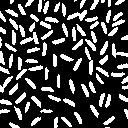
(a) Ground Truth

(b) Input Image

(c) MPLP-CP-v2

(d) SDBC

Figure 5: Image deconvolution on a $128\times 128$ image, which is convoluted by a $32\times 32$ Gaussian kernel. With the same running time, the result of SDBC is much better than MPLP-CP-v2.

In this paper, we refer to image deconvolution as the task of reconstructing an image from its convolution with a known blurring kernel. Raj and Zabih Raj and Zabih (2005) formulated the deconvolution to a MAP-MRF inference problem with unary and non-submodular pairwise energy functions. The connectivity increases with the growth in kernel size. We use two binary images and generate the deconvolution models with different kernel sizes ($3\!\times\!3$, $5\!\times\!5$ and $7\!\times\!7$). QPBO is applied on the six deconvolution models to reduce the graph size, and then SDBC, MPLP-CP-v2 and DAOOPT are applied on the reduced graphs. We also report the results of QPBO and LSA-TR Gorelick et al. (2014) with Euclidean or Hamming distance. LSA-TR is repeated (around $8000$ times) with random initializations until the $20$-minute time limit is used up. ICM is performed as a post-processing procedure for all the evaluated methods. Table 3 shows the primary evaluation results within the runtime limits of $20$ minutes, $1$ hour and $24$ hours. DAOOPT did not give solutions within the $24$ hours, so its result is omitted. Within $20$ minutes, MPLP-CP-v2 converges quickly to the exact MAP solutions for the two models with respect to $3\times 3$ kernel. But it does not converge for the rest four models with larger kernel sizes and higher connectivity. ILP fails to solve any of the six instances exactly within $24$ hours. LSA-TR and QPBO provide non-optimal solutions using a much shorter time. On the other hand, SDBC gives the best upper-bounds on all the $6$ instances within any of the three time limits, and is able to solve $5$ instances exactly (the model with respect to “ABCD” and $7\!\times\!7$ is not solved exactly by SDBC).

Fig. 4 illustrates the images recovered by SDBC and MPLP-CP-v2 with respect to $7\!\times\!7$ kernels within $20$ minutes. For image “1234”, SDBC achieves the energy value of $-478.07$ and the recovery accuracy of $87.4\%$, which are better than those given by MPLP-CP-v2 ($-474.19$ and $85.6\%$) respectively. Similarly for image “ABCD”, SDBC also performs better than MPLP-CP-v2, in terms of energy value ($-416.63$ vs. $-410.82$) and accuracy ($87.5\%$ vs. $86.0\%$).

We also evaluate algorithms on a larger image (Fig. 5). The binary ground truth image is convoluted by a $32\times 32$ Gaussian kernel. The corresponding MRF problem is large: $16384$ variables and $13130296$ edges, so we use a parallel eigen-solver, PLASMA. The last image shows the deconvolution result of SDBC using $5600$ seconds on $16$ cores. The result of MPLP-CP-v2 is demonstrated in the third image, using the same CPU hours. SDBC performs considerably better than MPLP-CP-v2.

5.3 Benchmarks

In this section, we evaluate the proposed algorithm on some MRF models in PIC2011 Elidan and Globerson (2011) and OpenGM Andres et al. (2014) benchmarks. The experimental results show that our method performs better than state-of-the-arts on these models. The chosen models are difficult for many conventional methods in that these inference tasks are non-submodular, densely connected and/or with unary terms.

5.3.1 PIC2011-ObjectDetection

Algorithm	Upper-bound	Lower-bound	$\#$Best-ub	$\#$Best-lb	$\#$Exact
Runtime $=20$min
SDBC	$\mathbf{-19302.83}$	$\mathbf{-19910.31}$	$\mathbf{34}$	$\mathbf{37}$	$0$
MPLP-CP-v1	$-18595.15$	$-24749.11$	$10$	$0$	$0$
MPLP-CP-v2	$-18905.71$	$-24624.95$	$13$	$0$	$0$
ILP	$-18247.73$	$-542806.60$	$8$	$0$	$0$
DAOOPT	$-19139.70$	$-\infty$	$17$	$0$	$0$
MPLP-BB	$-17838.86$	$-36904.82$	$11$	$0$	$0$
Runtime $=1$hr
SDBC	$\mathbf{-19303.06}$	$\mathbf{-19650.62}$	$\mathbf{35}$	$\mathbf{35}$	$0$
MPLP-CP-v1	$-18985.04$	$-22312.83$	$17$	$1$	$0$
MPLP-CP-v2	$-19231.27$	$-22260.29$	$19$	$1$	$0$
ILP	$-19049.54$	$-34838.62$	$15$	$0$	$0$
DAOOPT	$-19139.70$	$-\infty$	$17$	$0$	$0$
MPLP-BB	$-18227.13$	$-36804.25$	$10$	$0$	$0$
Runtime $=24$hr
SDBC	$\mathbf{-19313.25}$	$\mathbf{-19553.50}$	$\mathbf{36}$	$\mathbf{34}$	$\mathbf{3}$
MPLP-CP-v2	$-19270.70$	$-21138.12$	$22$	$3$	$0$
ILP	$-19221.27$	$-33888.65$	$22$	$0$	$0$
DAOOPT	$-19139.70$	$-\infty$	$16$	$0$	$0$

Table 4: PIC2011-ObjectDetection ($37$ instances, $60$ variables and $10$-$20$ labels for each instance). SDBC achieves the best upper-bounds and lower-bounds on most of instances within $20$ minutes, $1$ hour and $24$ hours. Exact solutions to $3$ instances are obtained by our algorithm.

There are $37$ models in the “Object-Detection” sub-category of the PIC2011 challenge, which are fully-connected, lacking in unary terms and have $60$ nodes and $10/15/20$ states per node. SDBC is compared with MPLP-CP-v1, MPLP-CP-v2, ILP, DAOOPT and MPLP-BB, among which DAOOPT is the winner of the PIC2011 challenge.

The primary results are shown in Table 4. The upper-bounds and lower-bounds of different methods are compared under three running-time limits: $20$ minutes, $1$ hour and $24$ hour. Our method achieves the best upper- and lower-bounds for most of the $37$ models under all time limits. DAOOPT is the second best method within $20$ minites, while MPLP-CP-v2 becomes better than DAOOPT within $1$ hour. ILP performs poorly within the runtime limit of $20$ minutes, while it becomes the second best in terms of the number of best upper-bounds ($22$, the same as MPLP-CP-v2).

In particular, all the evaluated methods do not converge to global optimal solutions on these models, except that SDBC gives exact solutions to three of the $37$ models.

5.3.2 OpenGM-ChineseChar

Algorithm	Upper-bound	Lower-bound	$\#$Best-ub	$\#$Best-lb	$\#$Exact	Runtime (s)
SDBC	$-49546.3380$	$\mathbf{-49558.9258}$	$\mathbf{84}$	$\mathbf{85}$	$44$	$2332.18$
MCBC	$\mathbf{-49550.0972}$	$-49612.3817$	$72$	$57$	$\mathbf{56}$	$2053.89$
ILP	$-49547.4144$	$-50061.1506$	$59$	$0$	$0$	$3553.71$
LSA-TR(euc.)	$-49548.0996$	$-\infty$	$28$	$0$	$0$	$\mathbf{0.05}$
LSA-TR(ham.)	$-49536.7646$	$-\infty$	$1$	$0$	$0$	$0.06$
QPBO	$-49501.9531$	$-50119.3835$	$0$	$0$	$0$	$0.17$

Table 5: OpenGM-ChineseChar ($100$ instances, $8000$ variables and $2$ labels for each instance). For fair comparison, all the combinatorial methods (SDBC, MCBC and ILP) are evaluated on graphs reduced by QPBO. The results of all algorithms except SDBC are obtained from Kappes et al. (2015). Within $1$ hour, SDBC solves $44$ instances exactly and achieves the best upper-bounds and lower-bounds on over $80\%$ instances.

The graphical model for Chinese character inpaining in the OpenGM benchmarks contains non-submoduar terms, such that graph cuts based methods cannot give exact solutions in general. It is shown in Kappes et al. (2015) that applying combinatorial algorithms (like MCBC Bonato et al. (2014) and ILP IBM (2015)) on the models reduced by QPBO achieves the best performance. Likewise, we also apply SDBC on the models reduced by QPBO and achieve comparable results. Within one hour, our method solves $44$ out of the $100$ instances exactly, which is only worse than the specialized solver, MCBC. Note that MCBC utilizes more complicated tightening constraints and rounding approach than ours. On the other hand, our method is better than all the other methods (including MCBC) in terms of the number of best upper-bounds ($84$) and lower-bounds ($85$). In particular, SDBC achieves better lower-bounds on those instances the LP methods (MCBC and ILP) are loose, which demonstrate the potential of SDBC in solving these instances exactly. To validate this potential, we run SDBC for $4$ hours and find that it gives global optimal solutions of $80$ instances.

5.3.3 OpenGM-ModularityClustering

Algorithm	Upper-bound	Lower-bound	$\#$Best-ub	$\#$Best-lb	$\#$Exact	Runtime (s)
SDBC	$\mathbf{-0.4913}$	$\mathbf{-0.4939}$	$\mathbf{6}$	$\mathbf{6}$	$\mathbf{5}$	$1500.26$
KL	$-0.4860$	$-\infty$	$2$	$0$	$0$	$\mathbf{0.01}$
MCR-CCFDB-OWC	$-0.4400$	$-0.5021$	$5$	$5$	$\mathbf{5}$	$601.38$
MCI-CCFDB-CCIFD	$-0.4652$	$-0.4962$	$5$	$5$	$\mathbf{5}$	$602.75$
MCI-CCI	$-0.4312$	$-0.5158$	$4$	$4$	$4$	$1207.07$
MCI-CCIFD	$-0.4399$	$-0.5176$	$4$	$4$	$4$	$1204.03$

Table 6: OpenGM-ModularityClustering ($6$ instances, $34$-$115$ variables and $34$-$115$ labels for each instance). As the top-performing algorithms (MCR-CCFDB-OWC and MCI-CCFDB-CCIFD) in Kappes et al. (2015), SDBC solves $5$ instances exactly. On the remaining largest instance, our method achieves the best lower-bound and upper-bound over all compared methods within $1$ hour.

The graphical models in this subclass is to find a clustering of a network maximizing the modularity. Although the six instances have small graph sizes ($34$ to $115$ variables), they are difficult due to the absence of unary terms and fully-connected graph structure.

It can be seen in Kappes et al. (2015) that the LP relaxation method with cycle and odd-wheel constraints (MCR-CCFDB-OWC) Kappes et al. (2011) and the LP/ILP method (MCI-CCFDB-CCIFD) Kappes et al. (2013b) perform the best on modularity clustering, which solve five of the six instances exactly. However, they do not converge on the largest instance within one hour. Kerninghan-Lin (KL) algorithm Kernighan and Lin (1970), a specialized efficient heuristic for clustering networks, offers a better solution than MCI and MCR on this instance. As MCR and MCI, our method also solves these five instances within one hour without branching (in other words, using only one bounding procedure). Moreover, SDBC provides the best solution (in terms of upper-bound) to the largest instance among all the evaluated approaches.

Dataset	Solution	$\#$Instances	$\#$Bounding	$\#$Pruned	$|\mathcal{Q}|$	Runtime
Deconvolution	Exact	$5$	$10.80$	$5.90$	$0.00$	$33332$
($6$ instances, runtime $\leq 24$hr)	Inexact	$1$	$19.00$	$6.00$	$8.00$	$84324$
Object-Detection	Exact	$3$	$75.67$	$38.33$	$0.00$	$33625$
($37$ instances, runtime $\leq 24$hr)	Inexact	$34$	$74.68$	$19.50$	$36.68$	$85631$
ChineseChar	Exact	$80$	$3.42$	$2.21$	$0.00$	$4347$
($100$ instances, runtime $\leq 4$hr)	Inexact	$20$	$3.45$	$1.00$	$2.45$	$12392$
Modularity-Clustering	Exact	$5$	$1.00$	$1.00$	$0.00$	$1063$
($6$ instances, runtime $\leq 1$hr)	Inexact	$1$	$1.00$	$0.00$	$2.00$	$3686$

Table 7: The average number of bounding iterations, pruned subproblems and unsolved subproblems in the queue $\mathcal{Q}$ for SDBC. The results for instances solved exactly and inexactly are summarized individually. SDBC uses $1$-$10$ bounding iterations to reach the exact solutions to most of instances on Deconvolution, ChineseChar and Modularity-Clustering. For Object-Detection, SDBC is able to solve $3$ instances exactly with less than $100$ bounding evaluations.

6 Conclusion

We have presented an efficient Branch-and-Cut method for MAP-MRF inference problems by taking the advantage of an efficient and tight SDP bounding procedure. The main contribution of the proposed method include: 1) A variety of linear tightening constraints have been incorporated in SDP relaxation to MAP problems, by using an efficient SDP solver and cutting-plane. 2) Several techniques have also been employed to make the cutting-plane and branch-and-bound more efficient, including model reduction, warm start and dropping inactive constraints. Experiments demonstrate that the proposed method performs very well, particularly for problems with high connectivity or weak unary potentials. These types of problems are difficult to solve by almost all other existing methods. Furthermore, our method usually provide good approximate solutions within the first several bounding procedures. In the experiments, we have compared the proposed approach with state-of-the-art methods. The results demonstrate the superior performance of our approach on the evaluated problems.

7 Appendix

7.1 Relationship between the Standard SDP Relaxation (19) and the Simplified Dual (29)

The Lagrangian dual of (19) can be expressed in the following general form:

$$\min_{\mathbf{u}} \quad\mathbf{u}^{\!\top}\mathbf{b}$$ (33a)

$$\mathrm{s.t.} \quad\mathbf{Z}=\mathbf{A}+\textstyle{\sum_{i=1}^{m}}u_{i}\mathbf{B}_{i}\succcurlyeq\mathbf{0},$$ (33b)

$$\quad u_{i}\geq 0,\forall i\in\mathcal{I}_{in}.$$ (33c)

The p.s.d. constraint (33b) can be replaced by a penalty function, which is considered as a measure of violation of this constraint. In our case, the penalty function is defined as $\mathrm{p}(\mathbf{u})=\lVert\min(\mathbf{0},{\boldsymbol{\lambda}})\rVert_{2}^{2}=\lVert\Pi_{\mathcal{S}^{n\!h\!+\!1}_{+}}(\mathbf{C}(\mathbf{u}))\rVert_{F}^{2}$, where ${\boldsymbol{\lambda}}$ is the vector of eigenvelues of $\mathbf{Z}$. We can find that if $\mathrm{p}(\mathbf{u})=0$, then $\mathbf{Z}\succcurlyeq\mathbf{0}$. Now the problem (33) can be transformed to

$$\min_{\mathbf{u}} \quad\mathbf{u}^{\!\top}\mathbf{b}+\frac{\gamma}{2}\lVert\Pi_{\mathcal{S}^{n\!h\!+\!1}_{+}}(\mathbf{C}(\mathbf{u}))\rVert_{F}^{2}$$ (34a)

$$\mathrm{s.t.} \quad u_{i}\geq 0,\forall i\in\mathcal{I}_{in},$$ (34b)

where $\gamma>0$ serves as a penalty parameter. With the increase of $\gamma$, the solution to (34) converges to that of (33). It is clear that (34) is equivalent to (29).

7.2 Proof of Propositions 1 and  2

Firstly, It is known Malick (2007); Wang et al. (2013) that the set of p.s.d. matrices with fixed trace $\Theta_{\eta}:=\{\mathbf{X}\succcurlyeq\mathbf{0}|\mathrm{trace}(\mathbf{X})\!=\!\eta\}$, $\forall\eta>0$ has the following property:

Theorem 7.1

(The spherical constraint). $\forall\eta>0,\forall\mathbf{X}\in\Theta_{\eta}$, we have $\lVert\mathbf{X}\rVert_{\!F\!}\!\leq\!\eta$, and $\lVert\mathbf{X}\rVert_{\!F\!}\!=\!\eta$ if and only if $\mathrm{rank}(\mathbf{X})\!=\!1$.

It is also shown in Wang et al. (2013) that the problem (29) is the Lagrangian dual of the following problem:

$$\min_{\mathbf{y},\mathbf{Y}}\,\, \mathrm{E}(\mathbf{y},\mathbf{Y})+\mathrm{g}_{\gamma}(\mathbf{y},\mathbf{Y})$$ (35a)

$$\mathrm{s.t.}\,\, \eqref{eq:sdprelax_cons1},\eqref{eq:sdprelax_cons2},\eqref{eq:sdprelax_cons3},\eqref{eq:sdprelax_cons4},\eqref{eq:sdprelax_cons5},\eqref{eq:tricons},\eqref{eq:cyccons},\eqref{eq:owccons},$$ (35b)

$$\Omega(\mathbf{y},\mathbf{Y})\succcurlyeq\mathbf{0},$$ (35c)

where $\mathrm{g}_{\gamma}(\mathbf{y},\mathbf{Y})=\frac{1}{2\gamma}(\lVert\Omega(\mathbf{y},\mathbf{Y})\rVert^{2}_{F}-(n+1)^{2})$.

Proof

of Proposition 1: ($i$) $\forall\mathcal{D}_{1}\!\subseteq\!\mathcal{D}_{2}\!\subseteq\!\mathcal{Z}^{n}$, $\exists\mathcal{F}_{in},\mathcal{F}_{eq}\in\{(p,i)\}_{p\in\mathcal{V},i\in\mathcal{Z}}$ such that $\mathcal{D}_{1}\!=\!\{\mathbf{x}\!\in\!\mathcal{D}_{2}\ |\ x_{p}\!\neq\!i,\forall(p,i)\!\in\!\mathcal{F}_{in};x_{p}\!=\!i,\forall(p,i)\!\in\!\mathcal{F}_{eq}\}$. Consequently, the difference between the SDCut primal formulation (35) with respect to $\mathcal{D}_{1}$ and $\mathcal{D}_{2}$ is that the one with respect to $\mathcal{D}_{1}$ contains the following additional linear constraints:

$$\left\{\begin{array}[]{ll}y_{p,i}=0,Y_{pi,qj}=Y_{qj,pi}=0,&\forall(p,i)\in\mathcal{F}_{in},\\ y_{p,i}=1,Y_{pi,qj}=Y_{qj,pi}=y_{q,j},&\forall(p,i)\in\mathcal{F}_{eq}.\end{array}\right.$$ (38)

Because of the strong duality, we know that $\mathrm{d}^{\star}_{\gamma}(\mathcal{D})$ equals to the optimal value of the corresponding primal problem (35). Then we have $\mathrm{d}^{\star}_{\gamma}(\mathcal{D}_{1})\geq\mathrm{d}^{\star}_{\gamma}(\mathcal{D}_{2})$, as the primal problem (35) with respect to $\mathcal{D}_{1}$ has more constraints than that with respect to $\mathcal{D}_{2}$.

($ii$) This proof is simple. As $\lvert{\mathcal{D}}\rvert=1$, there is only one point $\hat{\mathbf{x}}$ in the set $\mathcal{D}$ and $\mathrm{E}(\hat{\mathbf{x}})=\min_{\mathbf{x}\in\mathcal{D}}\mathrm{E}(\mathbf{x})$. Then the feasible set of (35) also contains a single point $\{\hat{\mathbf{y}},\hat{\mathbf{Y}}\}$ corresponding to $\hat{\mathbf{x}}$ by applying constraints as (38). Because $\lVert\Omega(\hat{\mathbf{y}},\hat{\mathbf{Y}})\rVert^{2}_{F}=(n+1)^{2}$, we have $\mathrm{d}^{\star}_{\gamma}(\mathcal{D})=\mathrm{E}(\hat{\mathbf{y}},\hat{\mathbf{Y}})=\min_{\mathbf{x}\in\mathcal{D}}\mathrm{E}(\mathbf{x})$.

Proof

of Proposition 2: $\{\mathbf{y}_{\gamma}^{\star},\mathbf{Y}_{\gamma}^{\star}\}$ is the optimal solution of (35) based on the strong duality, and $\mathrm{d}_{\gamma}(\mathbf{u}^{\star}_{\gamma})$ is the corresponding optimal objective value. Consider the following problem

$$\min_{\mathbf{y},\mathbf{Y}}\,\, \mathrm{E}(\mathbf{y},\mathbf{Y})+\mathrm{g}_{\gamma}(\mathbf{y},\mathbf{Y})$$ (39a)

$$\mathrm{s.t.}\,\, \Omega(\mathbf{y},\mathbf{Y})\succcurlyeq\mathbf{0},\,\mathrm{rank}(\Omega({\mathbf{y}_{\gamma}^{\star},\mathbf{Y}_{\gamma}^{\star}}))=1,$$ (39b)

$$\eqref{eq:sdprelax_cons1},\eqref{eq:sdprelax_cons2},\eqref{eq:sdprelax_cons3},\eqref{eq:sdprelax_cons4},\eqref{eq:sdprelax_cons5},\eqref{eq:tricons},\eqref{eq:cyccons},\eqref{eq:owccons},$$ (39c)

which adds a rank-$1$ constraint to the problem (35). Then $\mathrm{d}_{\gamma}(\mathbf{u}^{\star}_{\gamma})$ and $\{\mathbf{y}_{\gamma}^{\star},\mathbf{Y}_{\gamma}^{\star}\}$ are also optimal for the above problem. Note that the constraints (20), (21), $\Omega({\mathbf{y}_{\gamma}^{\star},\mathbf{Y}_{\gamma}^{\star}})\succcurlyeq\mathbf{0}$ and $\mathrm{rank}(\Omega({\mathbf{y}_{\gamma}^{\star},\mathbf{Y}_{\gamma}^{\star}}))=1$, force $\{\mathbf{y}_{\gamma}^{\star},\mathbf{Y}_{\gamma}^{\star}\}$ to be a vertex of $\mathcal{M}(\mathcal{G},\mathcal{Z})$. So the feasible set of (39) is $\mathcal{M}(\mathcal{G},\mathcal{Z})$. On the other hand, $\mathrm{g}_{\gamma}(\mathbf{y}_{\gamma}^{\star},\mathbf{Y}_{\gamma}^{\star})=0$ at $\mathrm{rank}(\Omega({\mathbf{y}_{\gamma}^{\star},\mathbf{Y}_{\gamma}^{\star}}))=1$ (Theorem 7.1), so the objective function of (39) is $\mathrm{E}(\mathbf{y},\mathbf{Y})$. In summary, the problem (39) is equivalent to the MAP problem $\displaystyle{\min_{\mathbf{y},\mathbf{Y}\in\mathcal{M}(\mathcal{G},\mathcal{Z})}}\mathrm{E}(\mathbf{y},\mathbf{Y})$. Then we have that $\mathbf{y}_{\gamma}^{\star},\mathbf{Y}_{\gamma}^{\star}$ yield the exact MAP solution and $\mathrm{d}_{\gamma}(\mathbf{u}^{\star}_{\gamma})$ is the minimum energy. The value of $\gamma$ does not affect the above results.

References

- Kappes et al. (2015) J. H. Kappes, B. Andres, F. A. Hamprecht, C. Schnörr, S. Nowozin, D. Batra, S. Kim, B. X. Kausler, T. Kröger, J. Lellmann, N. Komodakis, B. Savchynskyy, and C. Rother, “A comparative study of modern inference techniques for structured discrete energy minimization problems,” Int. J. Comp. Vis., 2015.
- Szeliski et al. (2008) R. Szeliski, R. Zabih, D. Scharstein, O. Veksler, V. Kolmogorov, A. Agarwala, M. Tappen, and C. Rother, “A comparative study of energy minimization methods for markov random fields with smoothness-based priors,” IEEE Trans. Pattern Anal. Mach. Intell., vol. 30, no. 6, pp. 1068–1080, 2008.
- Kumar et al. (2009) M. P. Kumar, V. Kolmogorov, and P. H. S. Torr, “An analysis of convex relaxations for MAP estimation of discrete MRFs,” J. Mach. Learn. Res., vol. 10, pp. 71–106, Jun 2009.
- Kolmogorov and Rother (2006) V. Kolmogorov and C. Rother, “Comparison of energy minimization algorithms for highly connected graphs,” in Proc. Eur. Conf. Comp. Vis., 2006, pp. 1–15.
- Givry et al. (2014) S. D. Givry, B. Hurley, D. Allouche, G. Katsirelos, B. O’Sullivan, and T. Schiex, “An experimental evaluation of CP/AI/OR solvers for optimization in graphical models,” in Congrès ROADEF’2014, Bordeaux, FRA, 2014.
- Boykov et al. (2001) Y. Boykov, O. Veksler, and R. Zabih, “Fast approximate energy minimization via graph cuts,” IEEE Trans. Pattern Anal. Mach. Intell., vol. 23, no. 11, pp. 1222–1239, 2001.
- Kolmogorov and Zabin (2004) V. Kolmogorov and R. Zabin, “What energy functions can be minimized via graph cuts?” IEEE Trans. Pattern Anal. Mach. Intell., vol. 26, no. 2, pp. 147–159, 2004.
- Kolmogorov and Rother (2007) V. Kolmogorov and C. Rother, “Minimizing nonsubmodular functions with graph cuts-a review,” IEEE Trans. Pattern Anal. Mach. Intell., vol. 29, no. 7, pp. 1274–1279, 2007.
- Rother et al. (2007) C. Rother, V. Kolmogorov, V. Lempitsky, and M. Szummer, “Optimizing binary MRFs via extended roof duality,” in Proc. IEEE Conf. Comp. Vis. Patt. Recogn., 2007, pp. 1–8.
- Pearl (1988) J. Pearl, Probabilistic reasoning in intelligent systems: networks of plausible inference. Morgan Kaufmann, 1988.
- Weiss and Freeman (2001) Y. Weiss and W. T. Freeman, “On the optimality of solutions of the max-product belief-propagation algorithm in arbitrary graphs,” IEEE Trans. Inf. Theory, vol. 47, no. 2, pp. 736–744, 2001.
- Sun et al. (2002) J. Sun, H.-Y. Shum, and N.-N. Zheng, “Stereo matching using belief propagation,” in Proc. Eur. Conf. Comp. Vis., 2002, pp. 510–524.
- Felzenszwalb and Huttenlocher (2006) P. F. Felzenszwalb and D. P. Huttenlocher, “Efficient belief propagation for early vision,” Int. J. Comp. Vis., vol. 70, no. 1, pp. 41–54, 2006.
- Aji et al. (1998) S. M. Aji, G. B. Horn, and R. J. Mceliece, “On the convergence of iterative decoding on graphs with a single cycle,” in Proc. ISIT, 1998.
- Weiss (2000) Y. Weiss, “Correctness of local probability propagation in graphical models with loops,” Neural Comp., vol. 12, no. 1, 2000.
- Bayati et al. (2005) M. Bayati, D. Shah, and M. Sharma, “Maximum weight matching via max-product belief propagation,” in Proc. IEEE Intl. Symp. on Information Theory. IEEE, 2005, pp. 1763–1767.
- Wainwright et al. (2005) M. J. Wainwright, T. S. Jaakkola, and A. S. Willsky, “MAP estimation via agreement on trees: message-passing and linear programming,” IEEE Trans. Inf. Theory, vol. 51, no. 11, pp. 3697–3717, 2005.
- Kolmogorov (2006) V. Kolmogorov, “Convergent tree-reweighted message passing for energy minimization,” IEEE Trans. Pattern Anal. Mach. Intell., vol. 28, no. 10, pp. 1568–1583, 2006.
- Kolmogorov and Wainwright (2005) V. Kolmogorov and M. J. Wainwright, “On the optimality of tree-reweighted max-product message-passing,” in Proc. Uncertainty in Artificial Intell., 2005.
- Shlezinger (1976) M. Shlezinger, “Syntactic analysis of two-dimensional visual signals in noisy conditions,” Kibernetika, vol. 4, pp. 113–130, 1976.
- Werner (2007) T. Werner, “A linear programming approach to max-sum problem: A review,” IEEE Trans. Pattern Anal. Mach. Intell., vol. 29, no. 7, pp. 1165–1179, 2007.
- Wainwright and Jordan (2008) M. J. Wainwright and M. I. Jordan, “Graphical models, exponential families, and variational inference,” Foundations and Trends® in Machine Learning, vol. 1, no. 1-2, pp. 1–305, 2008.
- Kumar et al. (2006) M. P. Kumar, P. H. Torr, and A. Zisserman, “Solving Markov random fields using second order cone programming relaxations,” in Proc. IEEE Conf. Comp. Vis. Patt. Recogn., vol. 1, 2006, pp. 1045–1052.
- Ravikumar and Lafferty (2006) P. Ravikumar and J. Lafferty, “Quadratic programming relaxations for metric labeling and Markov random field MAP estimation,” in Proc. Int. Conf. Mach. Learn., 2006, pp. 737–744.
- Globerson and Jaakkola (2007) A. Globerson and T. S. Jaakkola, “Fixing max-product: Convergent message passing algorithms for MAP LP-relaxations,” in Proc. Adv. Neural Inf. Process. Syst., 2007.
- Komodakis et al. (2011) N. Komodakis, N. Paragios, and G. Tziritas, “MRF energy minimization and beyond via dual decomposition,” IEEE Trans. Pattern Anal. Mach. Intell., vol. 33, no. 3, pp. 531–552, 2011.
- Kappes et al. (2010) J. H. Kappes, S. Schmidt, and C. Schnörr, “MRF inference by k-fan decomposition and tight lagrangian relaxation,” in Proc. Eur. Conf. Comp. Vis., 2010, pp. 735–747.
- Jojic et al. (2010) V. Jojic, S. Gould, and D. Koller, “Accelerated dual decomposition for MAP inference,” in Proc. Int. Conf. Mach. Learn., 2010, pp. 503–510.
- Kappes et al. (2012) J. H. Kappes, B. Savchynskyy, and C. Schnörr, “A bundle approach to efficient MAP-inference by lagrangian relaxation,” in Proc. IEEE Conf. Comp. Vis. Patt. Recogn., 2012, pp. 1688–1695.
- Ravikumar et al. (2010) P. Ravikumar, A. Agarwal, and M. J. Wainwright, “Message-passing for graph-structured linear programs: Proximal methods and rounding schemes,” J. Mach. Learn. Res., vol. 11, pp. 1043–1080, 2010.
- Martins et al. (2011a) A. F. Martins, N. A. Smith, E. P. Xing, P. M. Aguiar, and M. A. Figueiredo, “Augmenting dual decomposition for MAP inference,” in Proc. Int. Workshop on Optimization for Machine Learning, 2011.
- Martins et al. (2011b) A. F. Martins, M. A. Figueiredo, P. M. Aguiar, N. A. Smith, and E. P. Xing, “An augmented Lagrangian approach to constrained MAP inference,” in Proc. Int. Conf. Mach. Learn., 2011, pp. 169–176.
- Meshi and Globerson (2011) O. Meshi and A. Globerson, “An alternating direction method for dual MAP LP relaxation,” in Machine Learning and Knowledge Discovery in Databases. Springer, 2011, pp. 470–483.
- Hazan and Shashua (2010) T. Hazan and A. Shashua, “Norm-product belief propagation: Primal-dual message-passing for approximate inference,” IEEE Trans. Inf. Theory, vol. 56, no. 12, pp. 6294–6316, 2010.
- Johnson et al. (2007) J. K. Johnson, D. M. Malioutov, and A. S. Willsky, “Lagrangian relaxation for MAP estimation in graphical models,” 45th Ann. Allerton Conf. on Comm., Control and Comp., 2007.
- Savchynskyy et al. (2012) B. Savchynskyy, S. Schmidt, J. Kappes, and C. Schnörr, “Efficient MRF energy minimization via adaptive diminishing smoothing,” Proc. Uncertainty in Artificial Intell., 2012.
- Komodakis and Paragios (2008) N. Komodakis and N. Paragios, “Beyond loose LP-relaxations: Optimizing MRFs by repairing cycles,” in Proc. Eur. Conf. Comp. Vis., 2008, pp. 806–820.
- Werner (2008) T. Werner, “High-arity interactions, polyhedral relaxations, and cutting plane algorithm for soft constraint optimisation (MAP-MRF),” in Proc. IEEE Conf. Comp. Vis. Patt. Recogn., 2008, pp. 1–8.
- Sontag et al. (2008) D. Sontag, T. Meltzer, A. Globerson, T. S. Jaakkola, and Y. Weiss, “Tightening LP relaxations for MAP using message passing,” in Proc. Uncertainty in Artificial Intell., 2008.
- Batra et al. (2011) D. Batra, S. Nowozin, and P. Kohli, “Tighter relaxations for MAP-MRF inference: A local primal-dual gap based separation algorithm,” in Proc. Int. Conf. Artificial Intell. & Statistics, 2011, pp. 146–154.
- Johnson (2008) J. K. Johnson, “Convex relaxation methods for graphical models: Lagrangian and maximum entropy approaches,” Ph.D. dissertation, Massachusetts Institute of Technology, 2008.
- Sontag et al. (2012) D. Sontag, D. K. Choe, and Y. Li, “Efficiently searching for frustrated cycles in MAP inference,” in Proc. Uncertainty in Artificial Intell., 2012.
- Torr (2003) P. H. S. Torr, “Solving Markov random fields using semi definite programming,” in Proc. Int. Conf. Artificial Intell. & Statistics, 2003.
- Jordan and Wainwright (2003) M. J. Jordan and M. I. Wainwright, “Semidefinite relaxations for approximate inference on graphs with cycles,” in Proc. Adv. Neural Inf. Process. Syst., vol. 16, 2003, pp. 369–376.
- Olsson et al. (2007) C. Olsson, A. P. Eriksson, and F. Kahl, “Solving large scale binary quadratic problems: Spectral methods vs. semidefinite programming,” in Proc. IEEE Conf. Comp. Vis. Patt. Recogn., 2007, pp. 1–8.
- Schellewald and Schnörr (2005) C. Schellewald and C. Schnörr, “Probabilistic subgraph matching based on convex relaxation,” in Workshop of IEEE Conf. Comp. Vis. Patt. Recogn., 2005, pp. 171–186.
- Joulin et al. (2010) A. Joulin, F. Bach, and J. Ponce, “Discriminative clustering for image co-segmentation,” in Proc. IEEE Conf. Comp. Vis. Patt. Recogn., 2010.
- Peng et al. (2012) J. Peng, T. Hazan, N. Srebro, and J. Xu, “Approximate inference by intersecting semidefinite bound and local polytope,” in Proc. Int. Conf. Artificial Intell. & Statistics, 2012, pp. 868–876.
- Wang et al. (2013) P. Wang, C. Shen, and A. van den Hengel, “A fast semidefinite approach to solving binary quadratic problems,” in Proc. IEEE Conf. Comp. Vis. Patt. Recogn., 2013.
- Huang et al. (2014) Q. Huang, Y. Chen, and L. Guibas, “Scalable semidefinite relaxation for maximum a posterior estimation,” in Proc. Int. Conf. Mach. Learn., 2014.
- Frostig et al. (2014) R. Frostig, S. Wang, P. S. Liang, and C. D. Manning, “Simple MAP inference via low-rank relaxations,” in Proc. Adv. Neural Inf. Process. Syst., 2014, pp. 3077–3085.
- Sontag and Jaakkola (2007) D. Sontag and T. S. Jaakkola, “New outer bounds on the marginal polytope,” in Proc. Adv. Neural Inf. Process. Syst., 2007.
- Goemans and Williamson (1995) M. X. Goemans and D. P. Williamson, “Improved approximation algorithms for maximum cut and satisfiability problems using semidefinite programming,” J. ACM, vol. 42, pp. 1115–1145, 1995.
- Alizadeh et al. (1998) F. Alizadeh, J.-P. A. Haeberly, and M. L. Overton, “Primal-dual interior-point methods for semidefinite programming: convergence rates, stability and numerical results,” SIAM J. Optim., vol. 8, no. 3, pp. 746–768, 1998.
- Andersen et al. (2003) E. D. Andersen, C. Roos, and T. Terlaky, “On implementing a primal-dual interior-point method for conic quadratic optimization,” Math. Program., vol. 95, no. 2, pp. 249–277, 2003.
- Nesterov and Todd (1998) Y. E. Nesterov and M. J. Todd, “Primal-dual interior-point methods for self-scaled cones,” SIAM J. Optim., vol. 8, no. 2, pp. 324–364, 1998.
- Ye et al. (1994) Y. Ye, M. J. Todd, and S. Mizuno, “An O ()-iteration homogeneous and self-dual linear programming algorithm,” Mathematics of Operations Research, vol. 19, no. 1, pp. 53–67, 1994.
- Helmberg (1994) C. Helmberg, “An interior point method for semidefinite programming and max-cut bounds,” Ph.D. dissertation, Department of Mathematics, Graz University of Technology, 1994.
- Burer and Monteiro (2003) S. Burer and R. D. Monteiro, “A nonlinear programming algorithm for solving semidefinite programs via low-rank factorization,” Math. Program., vol. 95, no. 2, pp. 329–357, 2003.
- Arora et al. (2012) S. Arora, E. Hazan, and S. Kale, “The multiplicative weights update method: a meta-algorithm and applications.” Theory of Computing, vol. 8, no. 1, pp. 121–164, 2012.
- Arora et al. (2005) ——, “Fast algorithms for approximate semidefinite programming using the multiplicative weights update method,” in Proc. Annual IEEE Symposium on Foundations of Computer Science, 2005, pp. 339–348.
- Arora and Kale (2007) S. Arora and S. Kale, “A combinatorial, primal-dual approach to semidefinite programs,” in Proc. Annual ACM symposium on Theory of computing, 2007, pp. 227–236.
- Hazan (2008) E. Hazan, “Sparse approximate solutions to semidefinite programs,” in LATIN 2008: Theoretical Informatics, 2008, pp. 306–316.
- Garber and Hazan (2011) D. Garber and E. Hazan, “Approximating semidefinite programs in sublinear time,” in Proc. Adv. Neural Inf. Process. Syst., 2011, pp. 1080–1088.
- Laue (2012) S. Laue, “A hybrid algorithm for convex semidefinite optimization,” in Proc. Int. Conf. Mach. Learn., 2012, pp. 177–184.
- Malick et al. (2009) J. Malick, J. Povh, F. Rendl, and A. Wiegele, “Regularization methods for semidefinite programming,” SIAM J. Optim., vol. 20, no. 1, pp. 336–356, 2009.
- Zhao et al. (2010) X.-Y. Zhao, D. Sun, and K.-C. Toh, “A Newton-CG augmented Lagrangian method for semidefinite programming,” SIAM J. Optim., vol. 20, no. 4, pp. 1737–1765, 2010.
- Wen et al. (2010) Z. Wen, D. Goldfarb, and W. Yin, “Alternating direction augmented Lagrangian methods for semidefinite programming,” Mathematical Programming Computation, vol. 2, no. 3-4, pp. 203–230, 2010.
- Rockafellar (1973) R. T. Rockafellar, “A dual approach to solving nonlinear programming problems by unconstrained optimization,” Math. Program., vol. 5, no. 1, pp. 354–373, 1973.
- Shen et al. (2011) C. Shen, J. Kim, and L. Wang, “A scalable dual approach to semidefinite metric learning,” in Proc. IEEE Conf. Comp. Vis. Patt. Recogn., 2011, pp. 2601–2608.
- Sun et al. (2012) M. Sun, M. Telaprolu, H. Lee, and S. Savarese, “Efficient and exact MAP inference using branch and bound,” in Proc. Int. Conf. Artificial Intell. & Statistics, 2012.
- Otten and Dechter (2012) L. Otten and R. Dechter, “Anytime AND/OR depth-first search for combinatorial optimization,” AI Communications, vol. 25, no. 3, pp. 211–227, 2012.
- Rislock et al. (2012) N. Rislock, J. Malick, and F. Roupin, “Improved semidefinite bounding procedure for solving max-cut problems to optimality,” Math. Program., 2012.
- Armbruster et al. (2012) M. Armbruster, M. Fügenschuh, C. Helmberg, and A. Martin, “LP and SDP branch-and-cut algorithms for the minimum graph bisection problem: a computational comparison,” Mathematical Programming Computation, vol. 4, no. 3, pp. 275–306, 2012.
- Burer and Vandenbussche (2008) S. Burer and D. Vandenbussche, “A finite branch-and-bound algorithm for nonconvex quadratic programming via semidefinite relaxations,” Math. Program., vol. 113, no. 2, pp. 259–282, 2008.
- Dinh et al. (2010) T. P. Dinh, N. N. Canh, and H. A. Le Thi, “An efficient combined DCA and B&B using DC/SDP relaxation for globally solving binary quadratic programs,” Journal of Global Optimization, vol. 48, no. 4, pp. 595–632, 2010.
- Mars and Schewe (2012) S. Mars and L. Schewe, “SDP-package for SCIP,” TU Darmstadt, Tech. Rep., 2012.
- Helmberg and Weismantel (1998) C. Helmberg and R. Weismantel, “Cutting plane algorithms for semidefinite relaxations,” Fields Institute Communications, vol. 18, pp. 197–213, 1998.
- Helmberg et al. (2000) C. Helmberg, F. Rendl, and R. Weismantel, “A semidefinite programming approach to the quadratic knapsack problem,” Journal of combinatorial optimization, vol. 4, no. 2, pp. 197–215, 2000.
- Helmberg et al. (1996) ——, “Quadratic knapsack relaxations using cutting planes,” in Proceedings of the 5th International IPCO Conference on Integer Programming and Combinatorial Optimization, 1996, pp. 175–189.
- Helmberg and Rendl (1998) C. Helmberg and F. Rendl, “Solving quadratic (0, 1)-problems by semidefinite programs and cutting planes,” Mathematical Programming, vol. 82, no. 3, pp. 291–315, 1998.
- Helmberg et al. (1995) C. Helmberg, S. Poljak, F. Rendl, and H. Wolkowicz, “Combining semidefinite and polyhedral relaxations for integer programs,” in Proceedings of the 4th International IPCO Conference on Integer Programming and Combinatorial Optimization, 1995, pp. 124–134.
- Besag (1986) J. Besag, “On the statistical analysis of dirty pictures,” Journal of the Royal Statistical Society. Series B (Methodological), pp. 259–302, 1986.
- Horst et al. (2000) R. Horst, P. M. Pardalos, and N. Van Thoai, Introduction to global optimization. Springer, 2000.
- Hendrix et al. (2010) E. M. Hendrix, G. Boglárka et al., Introduction to nonlinear and global optimization. Springer, 2010.
- Achterberg et al. (2005) T. Achterberg, T. Koch, and A. Martin, “Branching rules revisited,” Operations Research Letters, vol. 33, no. 1, pp. 42–54, 2005.
- Land and Powell (1979) A. Land and S. Powell, “Computer codes for problems of integer programming,” Ann. Discrete Math., vol. 5, pp. 221–269, 1979.
- Linderoth and Savelsbergh (1999) J. T. Linderoth and M. W. Savelsbergh, “A computational study of search strategies for mixed integer programming,” INFORMS Journal on Computing, vol. 11, no. 2, pp. 173–187, 1999.
- Mitra (1973) G. Mitra, “Investigation of some branch and bound strategies for the solution of mixed integer linear programs,” Mathematical Programming, vol. 4, no. 1, pp. 155–170, 1973.
- Barahona and Mahjoub (1986) F. Barahona and A. R. Mahjoub, “On the cut polytope,” Mathematical programming, vol. 36, no. 2, pp. 157–173, 1986.
- Deza et al. (1992) M. Deza, M. Grötschel, and M. Laurent, “Clique-web facets for multicut polytopes,” Mathematics of Operations Research, vol. 17, no. 4, pp. 981–1000, 1992.
- Chopra and Rao (1993) S. Chopra and M. R. Rao, “The partition problem,” Mathematical Programming, vol. 59, no. 1-3, pp. 87–115, 1993.
- Deza and Laurent (1997) M. Deza and M. Laurent, “Geometry of cuts and metrics, volume 15 of algorithms and combinatorics,” 1997.
- Zhu et al. (1997) C. Zhu, R. H. Byrd, P. Lu, and J. Nocedal, “L-BFGS-B: Fortran subroutines for large-scale bound constrained optimization,” ACM T. Math. Softw., 1997.
- Kovtun (2011) I. Kovtun, “Sufficient condition for partial optimality for (max,+)-labeling problems and its usage,” Control systems and Computers, vol. 2, 2011.
- Swoboda et al. (2013) P. Swoboda, B. Savchynskyy, J. Kappes, and C. Schnörr, “Partial optimality via iterative pruning for the potts model,” in SSVM, 2013.
- Kohli et al. (2008) P. Kohli, A. Shekhovtsov, C. Rother, V. Kolmogorov, and P. Torr, “On partial optimality in multi-label mrfs,” in Proc. Int. Conf. Mach. Learn., 2008, pp. 480–487.
- Windheuser et al. (2012) T. Windheuser, H. Ishikawa, and D. Cremers, “Generalized roof duality for multi-label optimization: optimal lower bounds and persistency,” in Proc. Eur. Conf. Comp. Vis., 2012, pp. 400–413.
- Swoboda et al. (2014) P. Swoboda, B. Savchynskyy, J. H. Kappes, and C. Schnörr, “Partial optimality by pruning for map-inference with general graphical models,” in Proc. IEEE Conf. Comp. Vis. Patt. Recogn., 2014, pp. 1170–1177.
- Shekhovtsov (2014) A. Shekhovtsov, “Maximum persistency in energy minimization,” in Proc. IEEE Conf. Comp. Vis. Patt. Recogn., 2014, pp. 1162–1169.
- Shekhovtsov et al. (2015) A. Shekhovtsov, P. Swoboda, B. Savchynskyy, I. used by Alahari et al., “Maximum persistency via iterative relaxed inference with graphical models,” in Proc. IEEE Conf. Comp. Vis. Patt. Recogn., 2015, pp. 521–529.
- Alahari et al. (2008) K. Alahari, P. Kohli, and P. H. Torr, “Reduce, reuse & recycle: Efficiently solving multi-label MRFs,” in Proc. IEEE Conf. Comp. Vis. Patt. Recogn., 2008, pp. 1–8.
- Kappes et al. (2013a) J. H. Kappes, M. Speth, G. Reinelt, and C. Schnörr, “Towards efficient and exact MAP-inference for large scale discrete computer vision problems via combinatorial optimization,” in Proc. IEEE Conf. Comp. Vis. Patt. Recogn., 2013, pp. 1752–1758.
- Topkis (1982) D. Topkis, “A cutting-plane algorithm with linear and geometric rates of convergence,” Journal of Optimization Theory and Applications, vol. 36, no. 1, pp. 1–22, 1982.
- Joachims et al. (2009) T. Joachims, T. Finley, and C.-N. J. Yu, “Cutting-plane training of structural svms,” Machine Learning, vol. 77, no. 1, pp. 27–59, 2009.
- Horst and Tuy (2013) R. Horst and H. Tuy, Global optimization: Deterministic approaches. Springer, 2013.
- Gorelick et al. (2014) L. Gorelick, Y. Boykov, O. Veksler, I. B. Ayed, and A. Delong, “Local submodular approximations for binary pairwise energies,” in Proc. IEEE Conf. Comp. Vis. Patt. Recogn., 2014.
- Elidan and Globerson (2011) G. Elidan and A. Globerson, “The probabilistic inference challenge (PIC2011),” http://www.cs.huji.ac.il/project/PASCAL/, 2011.
- IBM (2015) IBM, “ILOG CPLEX optimizer,” http://www-01.ibm.com/software/integration/optimization/cplex-optimizer/, 2015.
- Kernighan and Lin (1970) B. Kernighan and S. Lin, “An efficient heuristic procedure for partitioning graphs,” The Bell Systems Technical Journal, vol. 49, no. 2, pp. 291–307, 1970.
- Bonato et al. (2014) T. Bonato, M. Jünger, G. Reinelt, and G. Rinaldi, “Lifting and separation procedures for the cut polytope,” Mathematical Programming, vol. 146, no. 1-2, pp. 351–378, 2014.
- Kappes et al. (2011) J. H. Kappes, M. Speth, B. Andres, G. Reinelt, and C. Schnörr, “Globally optimal image partitioning by multicuts,” in Energy Minimization Methods in Computer Vision and Pattern Recognition, 2011, pp. 31–44.
- Kappes et al. (2013b) J. H. Kappes, M. Speth, G. Reinelt, and C. Schnörr, “Higher-order segmentation via multicuts,” arXiv preprint arXiv:1305.6387, 2013.
- Andres et al. (2014) B. Andres, T. Beier, and J. H. Kappes, “OpenGM2,” http://hci.iwr.uni-heidelberg.de/opengm2/, 2014.
- Tütüncü et al. (2003) R. H. Tütüncü, K. C. Toh, and M. J. Todd, “Solving semidefinite-quadratic-linear programs using SDPT3,” Math. Program., vol. 95, no. 2, pp. 189–217, 2003.
- Kim and Lee (2011) W. Kim and K. M. Lee, “A hybrid approach for MRF optimization problems: Combination of stochastic sampling and deterministic algorithms,” Comp. Vis. Image Understanding, vol. 115, no. 12, pp. 1623–1637, 2011.
- Liu et al. (2015) F. Liu, G. Lin, and C. Shen, “CRF learning with CNN features for image segmentation,” Pattern Recognition, 2015.
- Wang et al. (2015) P. Wang, C. Shen, and A. V. D. Hengel, “Efficient SDP inference for fully-connected CRFs based on low-rank decomposition,” in Proc. IEEE Conf. Comp. Vis. Patt. Recogn., 2015.
- Raj and Zabih (2005) A. Raj and R. Zabih, “A graph cut algorithm for generalized image deconvolution,” in Proc. IEEE Int. Conf. Comp. Vis., 2005.
- Malick (2007) J. Malick, “The spherical constraint in boolean quadratic programs,” J. Global Optimization, vol. 39, no. 4, pp. 609–622, 2007.