Valley Order and Loop Currents in Graphene on Hexagonal Boron Nitride

Abstract

In this letter, we examine the role of Coulomb interactions in the emergence of macroscopically ordered states in graphene supported on hexagonal boron nitride substrates. Due to incommensuration effects with the substrate and interactions, graphene can develop gapped low energy modes that spatially conform into a triangular superlattice of quantum rings. In the presence of these modes, we show that Coulomb interactions lead to spontaneous formation of chiral loop currents in bulk and to macroscopic spin-valley order at zero temperature. We show that this exotic state breaks time reversal symmetry and can be detected with interferometry and polar Kerr measurements.

Introduction. In spite of the presence of quasiparticles with Dirac cone spectrum Antonio , the emergence of topological order in graphene is hindered by the fermionic doubling problem, where electrons have a four-fold degeneracy in valleys and spins Haldane . Due to the vanishingly small density of states (DOS) at the Dirac points, many-body instabilities in general are quantum critical and require strong coupling regimes Kotov . We argue that one promising possibility to generate many body states that lift the fermionic degeneracy and break time reversal symmetry (TRS) is to use substrates to reconstruct the DOS of graphene near the Dirac points into nearly flat bands.

In incommensurate two-layer crystals with honeycomb structure, the Dirac points are protected by a combination of parity and TRS Fu . On top of hexagonal boron nitride (BN), where inversion symmetry is broken, graphene can open a gap in the spectrum of the order of $\sim 20-50$meV Kindermann ; Justin ; Jung ; Pablo , as recently observed in transport measurements Hunt . Due to the 1.8% lattice mismatch between graphene and its substrate Giovannetti ; Yankowitz ; Yang and possible twisted configurations between the two Giovannetti ; Yankowitz ; Yang ; Sachs ; Wallbank , BN creates local potentials in graphene which modulate with the same periodicity of the Moire pattern created by the two incommensurate structures (Fig.1a) commensuration . In the continuum limit, the Hamiltonian of graphene in the presence of the BN substrate can be generically written as

$$\mathcal{H}=\int\mbox{d}^{2}r\sum_{\sigma}\sum_{\nu=\pm}\,\Psi_{\nu\sigma}^{\dagger}(\mathbf{r})[-vi\nabla\cdot\vec{\sigma}_{\nu}+\hat{A}_{\nu}(\mathbf{r})]\Psi_{\nu\sigma}(\mathbf{r})\,,$$ (1)

where $\Psi_{\nu}=(\psi_{\nu a},\psi_{\nu b})$ is a two component spinor in the sublattice space in a given valley, $\vec{\sigma}_{\nu}=(\nu\sigma_{1},\sigma_{2})$ are the Pauli matrices defined for each valley ($\nu=\pm$), $v=6\mbox{eV}\AA$ is the Fermi velocity, $\sigma=\uparrow\downarrow$ indexes the spin and $\hat{A}_{\nu}(\mathbf{r})=\mu(\mathbf{r})\sigma_{0}+\nu\mathbf{A}(\mathbf{r})\cdot\vec{\sigma}_{\nu}+M(\mathbf{r})\sigma_{3}$ are the local scalar, vector and mass term potentials induced by the BN substrate, which spatially modulate with the Moire pattern. In leading order, $\hat{A}_{\nu}(\mathbf{r})\approx\sum_{j=1}^{3}\cos(\mathbf{G}_{j}\cdot\mathbf{r})\,\hat{A}_{\nu}$, where $\mathbf{G}_{j}$ are the reciprocal lattice vectors in the Brillouin zone of the extended unit cell, and $\hat{A}_{\nu}$ parametrizes the amplitudes of modulating potentials.

As shown in previous tight binding models Kindermann ; SM , the regions where the mass term changes sign forms a lattice of disconnected quantum rings separating regions with opposite topological charges Volovik , as shown in Fig. 1b. In the presence of interactions, the amplitude of the induced mass term is $M\equiv\mbox{max}[M(\mathbf{r})]\approx 50-100$meV SM ; note4 for a Moire supercell with up to $140\mbox{\AA}$ in size Giovannetti ; Yankowitz ; Yang . The real space topology of those lines describes an insulating state in the bulk, unlike in twisted graphene bilayers, where inversion symmetry is restored and those gapless lines percolate into a metallic state with Dirac-like quasiparticles Kindermann ; Joao .

Figure 1: a) Moire pattern of graphene on top of boron nitride. b) Periodic mass term potentials $M(\mathbf{r})$ induced on graphene by the BN substrate. Solid rings: regions where the mass potential $M(\mathbf{r})$ crosses zero and changes sign SM .

Those 1D circular domain walls can contain gapped low energy modes when the amplitude of the induced mass term $M$ is larger than the finite size gap $\approx v/(2\pi a)$ set by the radius of the rings note . In this regime, we find that Coulomb interactions lead to spontaneous valley and spin polarization in those quantum rings, which describe chiral loop currents in bulk. We develop an effective lattice model and show that interactions lead to the subsequent formation of macroscopic valley and spin polarized low energy bands at zero temperature. This exotic ordered state explicitly breaks TRS and describes a ferromagnetic superlattice of spin and valley local moments. We propose that the ferromagnetic valley order can be detected with interferometry experiments and through the polar Kerr effect, which measures the rotation of a linearly polarized beam of light reflected on the sample.

Toy model Hamiltonian. In the presence of Coulomb interactions, the mass term $M(\mathbf{r})$ is a relevant operator in the renormalization group sense, while the scalar term $\mu(\mathbf{r})$ and the vector potential term $\mathbf{A}(\mathbf{r})$ are not Foster . The latter are small compared to the mass term in the strong coupling regime of the problem, which will be assumed Justin . In this regime, the mass term is the only relevant term and behaves as a periodic function that changes sign in the nodal lines where $M(\mathbf{r})=0$.

In cylindrical coordinates, $\mathbf{r}=(r,\theta),$ the mass term profile for a single quantum ring can be approximated by a step function, namely $M(r>a)=-M(r<a)=M$, where $a$ is the radius of the quantum ring. The Hamiltonian matrix of a single ring can be written as $\hat{\mathcal{H}}(\mathbf{r})=\hat{\mathcal{H}}_{+}(\mathbf{r})\otimes\nu_{+}+\hat{\mathcal{H}}_{-}(\mathbf{r})\otimes\nu_{-}$, where $\nu_{\pm}=(v_{0}\pm\nu_{3})/2$ are the valley projection operators, with $\nu_{i}$ ($i=1,2,3$) as Pauli matrices,

$$\hat{\mathcal{H}}_{+}(\mathbf{r})=\left(\begin{array}[]{cc}M(r)&-i\mbox{e}^{-i\theta}(\partial_{r}-\frac{i}{r}\partial_{\theta})\\ -i\mbox{e}^{i\theta}(\partial_{r}+\frac{i}{r}\partial_{\theta})&-M(r)\end{array}\right),$$ (2)

is the Hamiltonian in valley $\nu=+$ and $\hat{\mathcal{H}}_{-}=\hat{\mathcal{H}}_{+}^{*}$ in the opposite valley (we set $v\to 1$). The eigenvectors that satisfy the equation $\hat{\mathcal{H}}(\mathbf{r})\Phi(\mathbf{r})=E\Phi(\mathbf{r})$ are the four component spinors $\Phi_{j,+}(\mathbf{r})=\left(\Psi_{j}(\mathbf{r}),\mathbf{0}\right)$ and $\Phi_{j,-}(\mathbf{r})=\left(\mathbf{0},\Psi_{j}^{*}(\mathbf{r})\right)$, where

$$\Psi_{j}(\mathbf{r})=\left(\begin{array}[]{c}F_{j}^{-}(r)\mbox{e}^{i(j-\frac{1}{2})\theta}\\ iF_{j}^{+}(r)\mbox{e}^{i(j+\frac{1}{2})\theta}\end{array}\right),$$ (3)

with $j=m+\frac{1}{2}$ the total angular momentum quantum number ($m\in\mathbb{Z}$), including orbital (valley) and pseudo-spin (sublattice) degrees of freedom. Imposing the proper boundary conditions at $r=a$ and $r\to\infty$, $F_{j}^{\pm}(r)=A_{j}^{\pm}I_{|j\pm\frac{1}{2}|}(r\sqrt{M^{2}-E_{j}^{2}})\theta(a-r)+B_{j}^{\pm}K_{|j\pm\frac{1}{2}|}(r\sqrt{M^{2}-E_{j}^{2}})\theta(r-a)$, with $I_{n}(x)$ and $K_{n}(x)$ as modified Bessel functions, and $A_{j}^{\pm},$ $B_{j}^{\pm}$ the proper coefficients (see Fig. 2a). For $Ma\gg 1$ the wave functions are sharply peaked at $r=a$, and the states are localized at the domain wall where the mass term changes sign. In the opposite regime, when $Ma$ is of the order 1, the electrons can tunnel across the center of the ring and their wavefunctions become extended over the area of each ring, as in a quantum dot. In any case, the energy spectrum of the $j$ energy level is set by the condition

$$\frac{1}{4M^{2}}\prod_{s=\pm 1}\partial_{a}\ln\frac{K_{|j+\frac{s}{2}|}(\sqrt{M^{2}-E_{j}^{2}}a)}{I_{|j+\frac{s}{2}|}(\sqrt{M^{2}-E_{j}^{2}}a)}=1,$$ (4)

which gives a discrete spectrum of gapped low energy modes confined inside the quantum rings, as shown in Fig. 2b as a function of $Ma$.

The energy spectrum inside the gap is particle hole symmetric, with $j=m+\frac{1}{2}>0$ describing positive energy states and $j<0$ describing negative energy ones. The red curves correspond to $|j|=\frac{1}{2}$ states, while the other three curves describe $|j|=\frac{3}{2},\,\frac{5}{2}$ and $\frac{7}{2}$ states respectively, the outer curves having higher $|j|$. In all cases, there is a critical value of $Ma$ below which a given mode dives in the continuum of the band outside the gap. Inside the gap, those discrete levels are sharply defined and describe the circular motion of electrons physically confined inside the quantum rings shown in Fig. 1b. All levels have four-fold degeneracy, with two spins and two valleys. Their spin and orbital degeneracies can be lifted by repulsive interactions, which can give rise to locally polarized states.

Valley and spin polarized states. The Coulomb interaction between the electrons is

$$\mathcal{H}_{C}=\frac{1}{2}\int\mbox{d}^{2}r\mbox{d}^{2}r^{\prime}\,\hat{\rho}(\mathbf{r})V(\mathbf{r}-\mathbf{r}^{\prime})\hat{\rho}(\mathbf{r}^{\prime}),$$ (5)

where $V(\mathbf{r}-\mathbf{r}^{\prime})=e^{2}/(\kappa|\mathbf{r}-\mathbf{r}^{\prime}|)$, with $e$ the electric charge, $\kappa\approx 2.5$ the dielectric constant due to the BN substrate and $\hat{\rho}(\mathbf{r})=\sum_{\sigma}\Theta_{\sigma}^{\dagger}(\mathbf{r})\Theta_{\sigma}(\mathbf{r})$ is a density operator defined in terms of the field operators $\Theta_{\sigma}(\mathbf{r})\equiv\sum_{\nu,j}\Phi_{\nu,j}(\mathbf{r})c_{\nu,\sigma,j},$ where $c_{\nu,\sigma,j}$ describes an annihilation operator with spin $\sigma$ on a given valley and angular momentum state $j=m+\frac{1}{2}$.

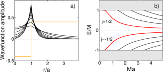
Figure 2: a) Amplitude of the wavefunctions around the domain wall set by the the quantum rings for $Ma$ ranging from $0.7$ to 3.5 for $|j|=\frac{1}{2}$. Orange line: profile of mass term potential $M(r)$ for a single quantum ring within the toy model. b) Gapped low energy modes $j=m+\frac{1}{2},$ for $m=-4,\,-3\ldots 3$ from bottom to the top curves. All modes are four-fold degenerate. The red lines indicate the $j=\pm\frac{1}{2}$ states.

The Coulomb interaction at the $j$-th level in a given quantum ring can be written as

$$\mathcal{H}_{U}=U\hat{n}_{\uparrow}\hat{n}_{\downarrow}+U\sum_{\sigma}\hat{n}_{+,\sigma}\hat{n}_{-,\sigma},$$ (6)

where

$$U=\int\mbox{d}^{2}r\mbox{d}^{2}r^{\prime}|\Phi_{\nu,j}(\mathbf{r})|^{2}V(\mathbf{r}-\mathbf{r}^{\prime})|\Phi_{\nu^{\prime},j}(\mathbf{r}^{\prime})|^{2}$$ (7)

is the valley independent Hubbard coupling and $\hat{n}_{\sigma}=\sum_{\nu}\hat{n}_{\nu,\sigma}$ describes the occupation of the $j$-th state in terms of $c$ operators ($j$ level indexes omitted). The Hubbard $U$ term is shown in Fig. 3a as a function of $Ma$ and shows a non-monotonic behavior, reflecting the crossover of the wavefunctions for $Ma\lesssim 1$, when the electrons can easily tunnel through the center of the quantum rings. At $Ma\lesssim 0.4$, the $|j|=\frac{1}{2}$ states merge the continuum, and the toy model description breaks down. The exchange interaction in a given ring is identically zero due to the orthogonality of the eigenspinors in different valleys, $\Phi_{+}^{\dagger}(\mathbf{r})\Phi_{-}(\mathbf{r})=0$ note1 . The problem of an isolated quantum ring in a given $j$ state is dual to the problem of a doubly degenerate orbital with spin $\frac{1}{2}$, and can be mapped in the Coqblin-Bladin model for two degenerate orbitals Coqblin .

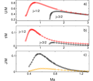
Figure 3: a) Scaling of the Hubbard energy $U$ and b) the hopping energy between nearest ring $t$ vs $Ma$. Red curves: $|j|=\frac{1}{2}$ levels; black curves: $|j|=\frac{3}{2}$. c) Exchange coupling $J$ (black circles) and superexchange coupling $t^{2}/U$ (orange) in $M$ units vs. $Ma$ in the $|j|=\frac{1}{2}$ state. For $0.4\lesssim Ma\lesssim 1$.1, the system shows ferromagnetic valley order (see text).

At the mean field level, the effective Hamiltonian of the $j$-th state with bare energy $E_{0}$ is $H_{L}=\sum_{\nu\sigma}E_{\nu\sigma}\hat{n}_{\nu,\sigma},$ where

$$E_{\nu,\sigma}=E_{0}+U\sum_{\nu^{\prime}}n_{\nu^{\prime},-\sigma}+Un_{-\nu,\sigma}$$

is the renormalized energy due to interactions. The occupation of the four degenerate states $n_{\nu,\sigma}$ $(\nu=\pm,\sigma=\uparrow\downarrow)$ in the $j$-th level can be calculated self-consistently from the Greens function of the localized $c$ electrons, $G_{\sigma,\nu}(\omega)=(\omega-E_{\sigma,\nu}+i\delta)^{-1},$ namely $n_{\nu,\sigma}=\langle\hat{n}_{\nu,\sigma}\rangle=-\frac{1}{\pi}\mbox{Im}\int_{-\infty}^{\mu}\mbox{d}\omega\,G_{\sigma,\nu}(\omega)$, with $\mu$ the chemical potential. When the repulsion $U$ is the dominant energy scale, the lowest energy solution is a state where $n_{\nu,\sigma}=N_{+}$ and $n_{\nu,-\sigma}=n_{-\nu,\sigma}=n_{-\nu,-\sigma}=N_{-}$, which is spin and valley polarized for $N_{+}\neq N_{-}$ Coqblin . In this regime,

$$N_{s}=\frac{1}{2}-\frac{1}{\pi}\mbox{arctan}\left(\frac{2N_{-}+N_{-s}-x}{y}\right),$$ (8)

with $s=\pm$, where $x=(\mu-E_{0})/U$ and $y=\delta/U$, with $\delta$ the level broadening. In the limit $y\to 0$, when the levels are sharply defined inside the gap, and $E_{0}<\mu<E_{0}+U$, the lowest energy solution is a maximally spin and valley polarized state with $N_{+}=1$ and $N_{-}=0$. This state describes a lattice of isolated quantum rings with random spin polarized circulating charge currents.

Nearly flat bands. The effective tight binding Hamiltonian for the $c$ electrons moving in a triangular superlattice of quantum rings is $\mathcal{H}_{eff}=\mathcal{H}_{t}+\sum_{i}\mathcal{H}_{U,i}+\sum_{\langle i,j\rangle}\mathcal{H}_{C,ij}$, where

$$\mathcal{H}_{t}=t\sum_{\langle ij\rangle}\sum_{\nu\sigma}c_{i,\nu,\sigma}^{\dagger}c_{j,\nu,\sigma}$$ (9)

is the kinetic energy of the electrons, with $c_{i}$ the annihilation operator for an electron in a quantum ring centered at $\mathbf{R}_{i}$, and $\langle ij\rangle$ indexes nearest neighbor (NN) sites. $t$ is the hopping energy betwen NN rings, $t_{ij}=\int\mbox{d}^{2}r\Phi_{\nu}^{\dagger}(\mathbf{r}_{i})\delta\hat{M}(\mathbf{r})\Phi_{\nu}(\mathbf{r}_{j})$, with $\mathbf{r}_{i}\equiv\mathbf{r}-\mathbf{R}_{i}$, where $\delta\hat{M}(\mathbf{r})=\delta M(\mathbf{r})\sigma_{3}\otimes\nu_{0}$ is the the mass potential that restores the periodicity of the superlattice when added to the step function potential $M(\mathbf{r})=M\,\mbox{sign}(r-a)$ due to one isolated quantum ring at the origin. The second term, $\mathcal{H}_{U,i}$, is the on-site Coulomb interaction (6) on a given site $i$ in the superlattice, and is defined by $\hat{n}_{i,\nu,\sigma}$ density operators. The third one, $\mathcal{H}_{C,ij}$, describes the Coulomb interaction (5) between different superlattice sites.

The hopping amplitude $t$ shown in Fig. 3b has a non-monotonic behavior as a function of $Ma$ which mimics the behavior of the Hubbard $U$ coupling, and is typically one order of magnitude smaller than the Coulomb interaction, $U/|t|\gtrsim 7$. In particular, for $M\approx 50-100$meV note4 and for a typical superlattice size of $3a\approx 140\mbox{\AA}$ Yankowitz ; Yang in graphene nearly aligned with BN, $Ma\in[0.4,\,0.8]$, which corresponds to a ratio $7\lesssim U/t\lesssim 9$. At quarter filling ($\mu=0$), that suggests that correlations keep the gapped 1D modes inside the rings strongly localized. In order to account for the macroscopic order of the chiral loop currents in bulk, we examine the electronic correlations among the rings.

As electrons hop between different superlattice sites, the on-site correlation tends to align either their valley or spin quantum numbers antiferromagnetically due to Pauli principle, in order to reduce the energy cost of the kinetic energy. In second order of perturbation theory, the super-exchange interaction among the rings is given by $\mathcal{H}_{S}=\mathcal{H}_{t}\mathcal{H}_{U}^{-1}\mathcal{H}_{t}+\mathcal{O}(t^{4})$, or equivalently $\mathcal{H}_{s}=-(t{}^{2}/U)\sum_{\langle ij\rangle}\sum_{\{\nu\}\{\sigma\}}c_{i,\nu,\sigma}^{\dagger}c_{j,\nu,\sigma}c_{j,\nu^{\prime},\sigma^{\prime}}^{\dagger}c_{i,\nu^{\prime},\sigma^{\prime}}$ Kugel . This term maps into the SU(4) Heisenberg Hamiltonian

$$\mathcal{H}_{s}=4\frac{t{}^{2}}{U}\sum_{\langle ij\rangle}\left(\frac{1}{4}+\boldsymbol{\tau}_{i}\cdot\boldsymbol{\tau}_{j}\right)\left(\frac{1}{4}+\mathbf{S}_{i}\cdot\mathbf{S}_{j}\right)$$ (10)

in a triangular lattice, where $\mathbf{S}_{i}$ is a spin $\frac{1}{2}$ operator on site $i$ and $\boldsymbol{\tau}_{i}$ the equivalent pseudo-spin operator, which acts in the valleys. This Hamiltonian is frustrated and is expected to describe a spin-orbital liquid in the ground state Penc .

The Coulomb interaction between rings, $\mathcal{H}_{C,ij}$, follows directly from Hamiltonian (5) by properly including the superlattice into the definition of the field operators $\Theta_{\sigma}(\mathbf{r})=\sum_{\nu,i}\Phi_{\nu}(\mathbf{r}_{i})c_{i,\nu\sigma}$. This term can be written explicitly in the form of the exchange interaction $\mathcal{H}_{e}=J\sum_{\langle ij\rangle}\sum_{\{\nu\}\{\sigma\}}c_{i,\nu,\sigma}^{\dagger}c_{j,\nu^{\prime},\sigma^{\prime}}^{\dagger}c_{i\nu^{\prime},\sigma^{\prime}}c_{j,\nu,\sigma},$ where $J>0$ is the exchange coupling, $J_{ij}\!=\!\frac{1}{2}\int\mbox{d}^{2}r\mbox{d}^{2}r^{\prime}\,\Phi_{\nu}^{\dagger}(\mathbf{r}_{i})\Phi_{\nu}(\mathbf{r}_{j})V(|\mathbf{r}-\mathbf{r}^{\prime}|)\Phi_{\nu^{\prime}}^{\dagger}(\mathbf{r}_{j}^{\prime})\Phi_{\nu^{\prime}}(\mathbf{r}_{i}^{\prime}),$ and can also be cast into the form of an SU(4) Heisenberg model

$$\mathcal{H}_{e}=-4J\sum_{\langle ij\rangle}\left(\frac{1}{4}+\boldsymbol{\tau}_{i}\cdot\boldsymbol{\tau}_{j}\right)\left(\frac{1}{4}+\mathbf{S}_{i}\cdot\mathbf{S}_{j}\right).$$ (11)

When $J>t{}^{2}/U$, the exchange coupling dominates and drives the system into a spin-valley ferromagnetic state with true long range order at zero temperature, giving rise to spin-valley polarized low energy bands. At strong enough coupling, those bands are expected to become nearly flat. In the corresponding midgap band formed by $j=-\frac{1}{2}$ levels, the spin-valley ferromagnetic state emerges for $0.4\lesssim Ma\lesssim 1.1$, as shown in Fig. 3c. In this interval, $J\lesssim 0.1M\sim 5-10$meV. Although knowing the exact polarization of the low energy bands requires self-consistently solving a non-trivial strongly correlated problem, when $U\gg t$ interactions are strong and lead to a net spin-valley polarization in the midgap states at zero temperature.

Experimental observation. In the valley ferromagnetic state, the loop currents in bulk break TRS and produce a ferromagnetic lattice of local magnetic moments $\approx\mu_{B}$, with $\mu_{B}$ a Bohr magneton. An external magnetic field $\mathbf{H}$ couples with the spin-valley moments through the Zeeman coupling, $\mathcal{H}_{Z}=-2\mu_{B}(\boldsymbol{\tau}+\mathbf{S})\cdot\mathbf{H}$. Due to the proximity of the ordered ground state at $T=0$, a very weak applied magnetic field $\mu_{B}H_{z}\sim 0.01k_{B}T$ can produce a large spin-valley magnetization $\sim 1\mu_{B}$ Antsygina . For instance, at temperatures $T\sim 0.01J/k_{B}\lesssim 1$K, the required applied field can be smaller than $H_{z}\lesssim 0.01$ T. In this regime, this state can generate a macroscopic flux $\Phi$ that is proportional to the spin-valley polarization. This flux can be detected with standard superconducting quantum interference devices placed on top of graphene Sepioni , as illustrated in Fig. 4a.

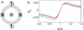
Figure 4: a) Magnetic flux $\Phi$ produced by the valley ferromagnetic state, measured by an interference device (gray region) on top of graphene. The supercurrent $I$ splits between two Josephson junctions (on green). b) Polar Kerr angle $\theta_{K}$ in radians versus photon energy $\omega$ normalized by the optical gap $\Delta$ for transitions between $j=\pm\frac{1}{2}$ energy flat bands. Curves for $Ma=0.5,\,0.6,\,0.7$ and $0.8$ (red) (see text).

When linearly polarized light is applied over an atomically thin medium that breaks TRS, the light polarization rotates by the Kerr angle $\theta_{K}(\omega)=8\pi/[c(n^{2}-1)]\mbox{Re}\,\sigma_{xy}(\omega)$ Nandkishore , where $\sigma_{xy}$ is the anomalous Hall conductivity Nagaosa , which is proportional to the valley polarization note3 , $c$ is the speed of light and $n\approx 2.5$ is the refraction index of the BN substrate. Within the toy model (2), the anomalous Hall conductivity can be derived by defining the electronic Green’s function $G_{\nu}(\mathbf{r},\mathbf{r}^{\prime},\omega)=\sum_{j,\mathbf{k}}\Phi_{\nu,j,\mathbf{k}}(\mathbf{r})\Phi_{\nu,j,\mathbf{k}}^{\dagger}(\mathbf{r}^{\prime})/(\omega-E_{j}+i\gamma)$ in terms of the Bloch waves in the superlattice for a given valley $\nu$, $\Phi_{\nu,j,\mathbf{k}}(\mathbf{r})=\sum_{i}\Phi_{\nu,j}(\mathbf{r}_{i})\mbox{e}^{i\mathbf{k}\cdot\mathbf{R}_{i}}$. For simplicity, we assume that $E_{j}$ is the energy of a dispersionless flat band indexed by the angular momentum state $j$ and $\gamma$ is the inverse of the quasiparticle lifetime.

The anomalous Hall conductivity in valley $\nu=+$ follows from the current-current correlation function $\Pi_{xy}(\mathbf{r},\mathbf{r}^{\prime},\omega)=e^{2}\mbox{tr}\!\int V_{+,x}G_{+}(\mathbf{r},\mathbf{r}^{\prime},\omega^{\prime})V_{+,y}G_{+}(\mathbf{r}^{\prime},\mathbf{r},\omega^{\prime}\!+\omega)\,\mbox{d}\omega^{\prime}/2\pi$, with $V_{\nu,i}=v(\sigma_{\nu,i}\otimes\nu_{0})$ Nagaosa . In momentum space, the optical Hall conductivity is $\sigma_{xy}(\omega)=(i/\omega)\lim_{\mathbf{q}\to 0}\Pi_{xy}(\mathbf{q},-\mathbf{q},\omega)$. The transitions between the valley polarized $j=\pm\frac{1}{2}$ bands dominate the Hall response for frequencies near the optical gap $\Delta=2E_{j=\frac{1}{2}}$. In this frequency range ($\sim 10^{13}$Hz), the zero temperature response is SM

$$\sigma_{xy}(\omega)\approx c_{0}^{2}\frac{e^{2}}{h}\frac{(\hbar v\Lambda)^{2}}{(\hbar\omega+i\gamma)^{2}-\Delta^{2}}$$ (12)

restoring $\hbar$, where $\Lambda\sim 2\pi/(3a)$ is the size of the Moire Brillouin zone and $c_{0}=\int\mbox{d}^{2}r\,F_{\frac{1}{2}}^{-}(r)F_{-\frac{1}{2}}^{+}(r)\approx 0.81$.

For $\gamma\sim 15$meV Zhou and $\hbar v\Lambda\approx 0.26$eV, which corresponds to a Moire unit cell of $140\mbox{\AA}$, the Kerr angle is $\theta_{K}\sim 10^{-2}$ radians for maximal valley polarization, as shown in Fig. 4b. For a weak valley magnetization of $0.1\mu_{B}$, the Kerr rotation is $\theta_{K}\sim 10^{-3}$, which is still very large. This effect that can be detected with THz/infrared Kerr experimental setups Zhou . In the visible range, Hall Kerr measurements are extremely sensitive and are able to detect rotations as small as $\theta_{K}\sim 10^{-9}$ radians Kapitulnik . By changing the occupation of the midgap states, the valley ferromagnetic order can be controlled with a gate voltage. This exotic state has clear experimental signatures and can lead to the experimental realization of valley order in graphene at low temperature and weak applied magnetic fields Amet .

Acknowledgements. We thank F. Guinea, E. Andrei, I. Martin, F. Mila, T. G. Rappoport, A. Del Maestro, K. Mullen, and A. Sandvik for discussions. BU acknowledges University of Oklahoma and NSF Career grant DMR-1352604 for support. VNK was supported by US DOE grant DE-FG02-08ER46512, and MK by NSF grant DMR-1055799.

Suplementary Materials for “Valley order and loop currents in graphene on hexagonal boron nitride”

Bruno Uchoa, Valeri N. Kotov and M. Kindermann

I Effective Hamiltonian in the Continuum

In the absence of interactions, the Hamiltonian of a two layer system is described by three terms,

$$\mathcal{H}=\mathcal{H}_{1}+\mathcal{H}_{2}+\mathcal{H}_{1-2}.$$ (13)

The first two terms describe the kinetic energy in each of the layers in separate, which in tight binding form is

$$\mathcal{H}_{l}=-t\sum_{\langle ij\rangle}\bar{\psi}_{l,a}^{\dagger}(\mathbf{R}_{i})\bar{\psi}_{l,b}(\mathbf{R}_{j})+(\mu_{l}+m_{l})\sum_{i}n_{l}(\mathbf{R}_{i})$$

with $l=1,2$ indexing the different layers, where $\bar{\psi}_{a}$ ($\bar{\psi}_{b})$ is an annihilation operator acting on sublattice $A$ ($B$) of each layer, $n_{l}$ is an on-site density operator on layer $l$, $t\sim 3$eV is the in-plane hopping energy, $\mu_{l}$ is the chemical potential, $m_{l}$ is the intrinsic mass gap of each layer and $\langle ij\rangle$ indicate sum over the nearest neighbor sites. Spin indexes will be omitted. For graphene on BN, we have $\mu_{1}=m_{1}=0$, $\mu_{2}\equiv V$ and $m_{2}\equiv m\neq 0$.

The $\bar{\psi}_{a,b}(\mathbf{r})$ operators can be written in a basis of Bloch wave functions as kindermann2 ; Mele2

$$\bar{\psi}_{x,l}(\mathbf{R})=\sum_{\nu=\pm}\phi_{x,l,\nu}(\mathbf{R})\,\psi_{x,l,\alpha}(\mathbf{R}),$$ (14)

where $\psi_{x}$ $(x=A,B)$ define the new fermionic operators,

$$\phi_{x,\nu,l}(\mathbf{R})=\frac{1}{\sqrt{3}}\sum_{a=1}^{3}\mbox{e}^{i\mathbf{K}_{\nu,l}^{a}\cdot(\mathbf{R}-\mathbf{R}_{x,l}^{0})}$$

is the corresponding Block wave function for each layer, $\mathbf{R}_{x,l}^{0}$ gives the position of a given arbitrary site on sublattice $x$ and layer $l$, and $\nu=\pm$ correspond to the two different valleys, each one represented by three distinct $\mathbf{K}_{\nu,l}^{a}$ vectors located at the corners of the Brillouin zone . In the continuum limit,

$$\mathcal{H}_{l}=\!\sum_{\nu=\pm}\int\!\!\mbox{d}^{2}r\,\Psi_{l,\nu}^{\dagger}(\mathbf{r})\!\left[-iv\vec{\sigma}_{\nu}\cdot\nabla+V_{l}\sigma_{0}+m_{l}\sigma_{3}\right]\!\Psi_{l,\nu}(\mathbf{r}),$$ (15)

where $\Psi=(\psi_{a},\psi_{b})$ is a two component spinor in the sublattice space of each layer, $\vec{\sigma}_{\nu}=(\nu\sigma_{1},\sigma_{2})$ are the Pauli matrices defined for each valley and $v=6\mbox{eV}\AA$ is the Fermi velocity, and $V_{l}$ are the local scalar potential in both layers.

The third term in (13), $H_{1-2}$, describes the electronic hopping between the two layers, which in the continuum limit is described by

$$\mathcal{H}_{1-2}=\int\mbox{d}^{2}r\,\sum_{\nu=\pm}\Psi_{1,\nu}^{\dagger}(\mathbf{r})\hat{t}_{\nu,\perp}(\mathbf{r})\Psi_{2,\nu}(\mathbf{r})+h.c,$$ (16)

where

$$t_{\nu,\perp}^{x,y}(\mathbf{r})=t_{\perp}\phi_{x,1,\nu}^{*}(\mathbf{r})\phi_{y,2,\nu}(\mathbf{r})$$

is the interlayer hopping matrix, with $t_{\perp}\sim 0.4$ eV the hopping amplitude Giovanetti2 .

The effective Hamiltonian of the gapless layer $1$ (graphene) can be computed directly by integrating out the electrons in the second layer, $\bar{\mathcal{H}}_{1}=\mathcal{H}_{1}+\delta\mathcal{H}_{1}$ where the second term describes the effective local potentials induced by layer 2. In lowest order in perturbation theory Kindermann3 ,

$$\delta\mathcal{H}_{1}=\int\mbox{d}\mathbf{r}\sum_{\nu=\pm}\Psi_{1,\nu}^{\dagger}(\mathbf{r})\hat{t}_{\nu,\perp}(\mathbf{r})\hat{M}\hat{t}_{\nu,\perp}^{\dagger}(\mathbf{r})\Psi_{1,\nu}(\mathbf{r}),$$ (17)

where

$$\hat{M}=\frac{1}{\omega-V+m}\left(\begin{array}[]{cc}\eta&0\\ 0&1\end{array}\right)$$ (18)

where $\omega$ is the interlayer applied bias voltage, and

$$\eta\equiv-\frac{m-V-\omega}{m+V+\omega}\approx-\frac{1.5-\omega}{3.1+\omega}.$$

In the first star approximationMele2 , where backscattering process are restricted to the first BZ of the extended unit cell, the spacial modulation of those fields can be approximated to a sum over the three reciprocal lattice vectors $\mathbf{G}_{j}$ of the extended unit cell kindermann2 ,

$$\hat{A}_{\nu}(\mathbf{r})=\hat{t}_{\nu,\perp}(\mathbf{r})\hat{M}\hat{t}_{\nu,\perp}^{\dagger}(\mathbf{r})\approx\sum_{j=1}^{3}\cos(\mathbf{G}_{j}\cdot\mathbf{r})\hat{A}_{\nu},$$ (19)

where $\hat{A}_{\nu}$ is in the form $\hat{A}_{\nu}\equiv\mu\sigma_{0}+\mathbf{A}\cdot\vec{\sigma}_{\nu}+M\sigma_{3}$.

For graphene at half filling on BN, the microscopic parameters can be extracted from ab initio calculations. The intrinsic BN gap is $m\approx 2.3$ eV and $V\approx 0.8$eV Giovanetti2 . At zero interlayer bias, $\eta=-0.5$, which describes Fig. 1 of the main text at small twist angles.

For $t_{\perp}\approx 0.4$eV and zero bias, the maximal allowed amplitude for the mass term is $M\approx t_{\perp}^{2}/(m-V)\sim 100$meV. In the absence of interactions, one may adopt a conservative estimate of $M\approx 50$ meV, which is consistent with recent ab initio results Sachs-1 . Many-body effects can significantly renormalize $M$ and make it substantially larger KotovSM ; Justin-1 . In the manuscript, we consider the effects of renormalized low energy bands corresponding to an amplitude of the mass term in the range $M\sim 50-100$meV.

II Anomalous Hall Conductivity

The Bloch wave functions for electrons in a lattice of quantum rings is

$$\Psi_{j,\mathbf{k}}(\mathbf{r})=\sum_{\mathbf{R}}\Psi_{j}(\mathbf{r}-\mathbf{R})\mbox{e}^{i\mathbf{k}\cdot\mathbf{R}}$$ (20)

where $\mathbf{R}$ indexes the superlattice sites, and

$$\Psi_{j}(\mathbf{r})=\left(\begin{array}[]{c}F_{j}^{-}(r)\mbox{e}^{i(j-\frac{1}{2})\theta}\\ iF_{j}^{+}(r)\mbox{e}^{i(j+\frac{1}{2})\theta}\end{array}\right),$$ (21)

is the wavefunction in a given ring on valley $v=+$. The real space Green’s function is

$$G(\mathbf{r},\mathbf{r}^{\prime},i\omega) = \sum_{j,\mathbf{k}}\frac{\Psi_{j,\mathbf{k}}(\mathbf{r})\Psi_{j,\mathbf{k}}^{\dagger}(\mathbf{r}^{\prime})}{i\omega-\epsilon_{j}}$$

$$= \sum_{j}\sum_{\mathbf{R}}\frac{\Psi_{j}(\mathbf{r}-\mathbf{R})\Psi_{j}^{\dagger}(\mathbf{r}^{\prime}-\mathbf{R})}{i\omega-\epsilon_{j}},$$

with $\epsilon_{j}$ the energy of a dispersionless flat band $j$. The Fourier transform of the Green’s function in momentum space is

$$G(\mathbf{p},\mathbf{p}^{\prime},i\omega)=\delta_{\mathbf{p},\mathbf{p}^{\prime}}\sum_{j}\int\!\mbox{d}\mathbf{r}\,\mbox{d}\mathbf{r}^{\prime}\frac{\Psi_{j}(\mathbf{r})\Psi_{j}^{\dagger}(\mathbf{r}^{\prime})}{i\omega-\epsilon_{j}}\,\mbox{e}^{i\mathbf{p}\cdot(\mathbf{r}-\mathbf{r}^{\prime})}.$$

The current-current correlation function is

$$\Pi_{xy}(\mathbf{q},\mathbf{q}^{\prime},i\omega)=\frac{e^{2}v^{2}}{\beta}\sum_{i\omega^{\prime}}\sum_{\mathbf{p},\mathbf{p}^{\prime}}\mbox{tr}\left[\sigma_{x}G(\mathbf{p}^{\prime}+\mathbf{q},\mathbf{p}-\mathbf{q}^{\prime},i\omega^{\prime}+i\omega)\sigma_{y}G(\mathbf{p},\mathbf{p}^{\prime},i\omega^{\prime})\right],$$ (22)

with $\beta$ the inverse of temperature. Accounting only for transitions between the $j=\pm\frac{1}{2}$ states, which are dominant at frequencies near the optical gap $\omega\sim 2\epsilon_{j=\frac{1}{2}},$

$$\Pi_{xy}(\mathbf{q},\mathbf{q}^{\prime},i\omega)\approx\frac{i}{4\pi}e^{2}(v\Lambda)^{2}c_{0}^{2}\,\delta_{\mathbf{q},-\mathbf{q}^{\prime}}\left[\frac{1}{i\omega-\epsilon_{\frac{1}{2}}+\epsilon_{-\frac{1}{2}}}+\frac{1}{i\omega+\epsilon_{\frac{1}{2}}-\epsilon_{-\frac{1}{2}}}\right]\left[n_{F}(\epsilon_{\frac{1}{2}})-n_{F}(\epsilon_{-\frac{1}{2}})\right]\mbox{e}^{i\mathbf{q}\cdot(\mathbf{r}-\mathbf{r}^{\prime})},$$ (23)

where $\Lambda\approx 2\pi/(3a)$ is a momentum cut-off set by the size of the Moire BZ, $c_{0}\equiv\int_{0}^{\infty}\mbox{d}^{2}r\,F_{\frac{1}{2}}^{-}(r)F_{-\frac{1}{2}}^{+}(r)\sim 0.81$, and $n_{F}$ is the Fermi distribution. The optical Hall conductivity follows from $\sigma_{xy}(\omega)=(i/\omega)\lim_{\mathbf{q}\to 0}\Pi_{xy}(\mathbf{q},-\mathbf{q},\omega+i0^{+})$.

References

(1)A. H. Castro Neto, N. M.
R. Peres, F. Guinea, K. Novoselov, A. Geim,Rev. Mod.
Phys.81, 109 (2009).
(2)F. D. M. Haldane, Phys. Rev. Lett. 61,
2015 (1988).
(3)V. N . Kotov, B. Uchoa, V. M. Pereira, F. Guinea,
and A. H. Casto Neto, Rev. Mod. Phys. 84, 1067 (2012).
(4)L. Fu and C. L. Kane, Phys. Rev. B 76, 045302
(2007).
(5)M. Kindermann, B. Uchoa, and D. L. Miller, Phys.
Rev. B 86, 115415 (2012).
(6)J. C. W. Song, A. V. Shytov, and L. S. Levitov, Phys.
Rev. Lett. 111, 266801 (2013).
(7)J. Jung, A. DaSilva, S. Adam, and A. H. MacDonald,
arXiv:1403.0496v1 (2014).
(8)P. San-Jose, A. Guti rrez, M. Sturla, F. Guinea, Phys.
Rev. B 90, 075428 (2014).
(9)B. Hunt, J. D. Sanchez-Yamagishi, A. F. Young, M. Yankowitz,
B. J. LeRoy, K. Watanabe, T. Taniguchi, P. Moon, M. Koshino, P. Jarillo-Herrero,
R. C. Ashoori, Science 340, 1427 (2013).
(10)G. Giovannetti, P. A. Khomyakov, G. Brocks,
P. J. Kelly, and J. van den Brink, Phys. Rev. B 76, 073103
(2007).
(11)M. Yankowitz, J. Xue, D. Cormode, J. D. Sanchez-Yamagishi,
K. Watanabe, T. Taniguchi, P. Jarillo-Herrero, P. Jacquod, B. J. LeRoy,
Nature Physics 8, 382–386 (2012).
(12)W. Yang, G. Chen, Z. Shi, C.-C. Liu, L. Zhang, G. Xie,
M. Cheng, D. Wang, R. Yang, D. Shi, K. Watanabe, T. Taniguchi, Y.
Yao, Y. Zhang, G. Zhang, Nature Mater. 12, 792 (2013).
(13)B. Sachs, T. O. Wehling, M. I. Katsnelson, and A.
I. Lichtenstein, Phys. Rev. B 84, 195414 (2011).
(14)J. R. Wallbank, A. A. Patel, M. Mucha-Kruczynski,
A. K. Geim, and V. I. Fal’ko, Phys. Rev. B 87,
245408 (2013).
(15)Recent experiments observed commensuration
effects, which were associated with topologically non trivial states.
See C. R. Woods et al., Nature Phys. 10 451, (2014);
J. C. W. Song, P. Samutpraphoot, L. S. Levitov, Xiv:1404.4019 (2014)
and R. V. Gorbachev et al., arXiv:1409.0113 (2014). We consider
the incommensurate regime observed in Hunt .
(16)See supplementary materials.
(17)In the non-interacting picture, 50meV
for large Moire unit cells SM . RG results indicate that ,
with Justin ; Kotov2 , and
sets the length scale of the RG flow, which stops at the size of the
Moire unit cell, with the lattice parameter.
Hence, . In experiment, the renormalization is
limited by infrared cut-offs set by disorder and screening from metallic
contacts.
(18)G. Volovik, The universe in a helium droplet
(Oxford, 2002).
(19) M. B. Lopes dos Santos, N. M. R. Peres, and A. H.
Castro Neto, Phys. Rev. Lett. 99, 256802 (2007).
(20)The index theorem sets the number of zero modes as
the difference in the topological charges on the two sides of a topological
domain wall. This result nevertheless holds up to finite size effects.
(21)M. Foster, I. Aleiner, Phys. Rev. B 77,
195413 (2008).
(22)V. N. Kotov, B. Uchoa and A. H. Castro Neto, Phys.
Rev. B 80, 165424 (2009).
(23) In Eq. (5), the exchange contribution for
two electrons in the same ring is ,
where .
(24)B. Coqblin, and A. Blandin, Advances in Physics
17, 281 (1968).
(25)K. I. Kugel and D. I. Khomskii, Sov. Phys. JETP 37,
725 (1973).
(26)K. Penc, M. Mambrini, P. Fazekas, and F. Mila, Phys.
Rev. B 68, 012408 (2003).
(27)T. N. Antsygina, M. I. Poltavskaya, I. I. Poltavsky,
and K. A. Chishko, Phys. Rev. B 77, 024407 (2008).
(28)M. Sepioni, R. R. Nair, S. Rablen, J. Narayanan,
F. Tuna, R. Winpenny, A. K. Geim, and I. V. Grigorieva, Phys. Rev.
Lett. 105, 207205 (2010).
(29)R. Nandkishore, L. Levitov, Phys. Rev. Lett.
107, 097402 (2011).
(30)N. Nagaosa, J. Sinova, S. Onoda, A. H. MacDonald,
N. P. Ong, Rev. Mod. Phys. 82, 1539 (2010).
(31)Since the spin-orbit coupling in graphene is tipically
small, the valley order should dominate the magneto-optical response.
(32)Y. Zhou, X. Xu, H. Fan, Z. Ren, X. Chen, and J. Bai,
J. Phys. Soc. Jap. 82, 074717 (2013).
(33)A. Kapitulnik, J. Xia, E. Schemm, A. Palevski,
New J. Phys. 11, 055060 (2009).
(34)F. Amet, J. R. Williams, K.Watanabe, T. Taniguchi,
and D. Goldhaber-Gordon, Phys. Rev. Lett. 110, 216601 (2012).

References

(1)M. Kindermann and P. N. First, Phys. Rev. B
83, 045425 (2011).
(2)E. J. Mele, Phys. Rev. B 84, 235439 (2011).
(3)G. Giovannetti, P. A. Khomyakov, G. Brocks,
P. J. Kelly, and J. van den Brink, Phys. Rev. B 76, 073103 (2007).
(4)M. Kindermann, B. Uchoa, and D. L. Miller, Phys.
Rev. B 86, 115415 (2012).
(5)B. Sachs, T. O. Wehling, M. I. Katsnelson, and A.
I. Lichtenstein, Phys. Rev. B 84, 195414 (2011).
(6)V. N. Kotov, B. Uchoa and A. H. Castro Neto, Phys.
Rev. B 80, 165424 (2009).
(7)J. C. W. Song, A. V. Shytov, and L. S. Levitov,
Phys. Rev. Lett. 111, 266801 (2013).