Tight Bounds for Learning a Mixture of Two Gaussians

Abstract

We consider the problem of identifying the parameters of an unknown mixture of two arbitrary $d$-dimensional gaussians from a sequence of independent random samples. Our main results are upper and lower bounds giving a computationally efficient moment-based estimator with an optimal convergence rate, thus resolving a problem introduced by Pearson (1894). Denoting by $\sigma^{2}$ the variance of the unknown mixture, we prove that $\Theta(\sigma^{12})$ samples are necessary and sufficient to estimate each parameter up to constant additive error when $d=1.$ Our upper bound extends to arbitrary dimension $d>1$ up to a (provably necessary) logarithmic loss in $d$ using a novel—yet simple—dimensionality reduction technique. We further identify several interesting special cases where the sample complexity is notably smaller than our optimal worst-case bound. For instance, if the means of the two components are separated by $\Omega(\sigma)$ the sample complexity reduces to $O(\sigma^{2})$ and this is again optimal.

Our results also apply to learning each component of the mixture up to small error in total variation distance, where our algorithm gives strong improvements in sample complexity over previous work. We also extend our lower bound to mixtures of $k$ Gaussians, showing that $\Omega(\sigma^{6k-2})$ samples are necessary to estimate each parameter up to constant additive error.

1 Introduction

Gaussian mixture models are among the most well-studied models in statistics, signal processing, and computer science with a venerable history spanning more than a century. Gaussian mixtures arise naturally as way of explaining data that arises from two or more homogeneous populations mixed in varying proportions. There have been numerous applications of gaussian mixtures in disciplines including astronomy, biology, economics, engineering and finance.

The most basic estimation problem when dealing with any mixture model is to approximately identify the parameters that specify the model given access to random samples. In the case of a gaussian mixture the model is determined by a collection of means, covariance matrices and mixture probabilities. A sample is drawn by first selecting a component according to the mixture probabilities and then sampling from the normal distribution specified by the corresponding mean and covariance. Already in 1894, Pearson [Pea94] proposed the problem of estimating the parameters of a mixture of two one-dimensional gaussians in the context of evolutionary biology. Pearson analyzed a population of crabs and found that a mixture of two gaussians faithfully explained the size of the crab “foreheads”. He concluded that what he observed was a mixture of two species rather than a single species and further speculated that “a family probably breaks up first into two species, rather than three or more, owing to the pressure at a given time of some particular form of natural selection.”

Fitting a mixture of two gaussians to the observed crab data was a formidable task at the time that required Pearson to come up with a good approach. His approach is based on the method of moments which uses the empirical moments of a distribution to distinguish between competing models. Given $n$ samples $x_{1},\dots,x_{n}$ the $k$-th empirical moment is defined as $\frac{1}{n}\sum_{i}x_{i}^{k}$, which for sufficiently large $n$ will approximate the true moment $\operatorname*{\mathbb{E}}x_{i}^{k}.$ A mixture of two one-dimensional gaussians has $5$ parameters so one might hope that $5$ moments are sufficient to identify the parameters. Pearson derived a ninth degree polynomial $p_{5}$ in the first $5$ moments and located the roots of this polynomial. Each root gives a candidate mixture that matches the first $5$ moments; there were two valid solutions, among which Pearson selected the one whose $6$-th moment was closest to the observed empirical $6$-th moment.

In this work, we extend the method proposed by Pearson and prove that the extended method reliably recovers the parameters of the unknown mixture. Moreover, we show that the sample complexity we achieve is essentially optimal. To illustrate the quantitative bound that we get, if the means and variances are separated by constants and the total variance of the mixture is $\sigma^{2},$ then we show that up to constant factors it is necessary and sufficient to use $\sigma^{12}$ samples to recover the parameters up to small additive error. Our work can be interpreted as providing an extension of Pearson’s 120-year old estimator that achieves an optimal convergence rate. We extend our result to arbitrary dimension $d$ using an apparently novel but surprisingly simple dimensionality reduction technique. This allows us to obtain the same sample complexity in any dimension up to a logarithmic loss in $d$, which we can also show is necessary.

Closely related to our results is an important recent work of Kalai, Moitra and Valiant [KMV10] who gave the first proof of a computationally efficient estimator with an inverse-polynomial convergence rate for the problem we consider. In particular, they show that six moments suffice to identify a mixture of two one-dimensional gaussians. Moreover, the result is robust in the sense that if the parameters of a mixture with variance $\sigma^{2}$ are separated by constants, then one of the first $6$ moments must differ by $1/\sigma^{66}.$ In particular, the first six empirical moments suffice provided that they’re within $1/\sigma^{66}$ of the true moments (which happens for $n\gg\sigma^{132}$). This then leads to an estimator up to some polynomial loss. They also show that a solution to the $1$-dimensional problem extends to any dimension $d$ up to some loss that’s polynomial in $d$ and $\sigma$ using a suitable dimensionality reduction technique. In contrast to their result which is within a polynomial factor of optimal, our result is within a constant factor of optimal in one dimension and within a $\log_{d}\log\sigma$ factor of optimal in $d$ dimensions.

1.1 Problem description

A mixture $F$ of two $d$-dimensional gaussians is specified by mixing probabilities $p_{1},p_{2}\geq 0$ such that $p_{1}+p_{2}=1,$ two means $\mu_{1},\mu_{2}\in\mathbb{R}^{d}$ and two covariance matrices $\Sigma_{1},\Sigma_{2}\in\mathbb{R}^{d\times d}.$ A sample from $F$ is generated by first picking an integer $i\in\{1,2\}$ from the distribution $(p_{1},p_{2})$ and then sampling from the $d$-dimensional gaussian measure $\mathrm{N}(\mu_{i},\Sigma_{i}).$

The variance $\sigma^{2}$ of a $1$-dimensional mixture of two gaussians is $p_{1}p_{2}(\mu_{1}-\mu_{2})^{2}+p_{1}\sigma_{1}^{2}+p_{2}\sigma_{2}^{2}$. For a $d$-dimensional mixture, it is useful to define its “variance” as the maximum variance of any coordinate,

$$\operatorname*{\mathbb{V}}(F)\,\stackrel{{\scriptstyle{\mathrm{def}}}}{{=}}\,p_{1}p_{2}\|\mu_{1}-\mu_{2}\|_{\infty}^{2}+p_{1}\|\Sigma_{1}\|_{\infty}+p_{2}\|\Sigma_{2}\|_{\infty}\,.$$ (1)

Given samples from $F$ our goal is to recover the parameters that specify the mixture up to small additive error; this is known as parameter distance. It is easy to see that we can only hope to recover the components of the mixture up to permutation. For simplicity it is convenient to combine the error in estimating the parameters:

Definition 1.1.

We say that mixture $\widehat{F}$ is $\epsilon$-close to mixture $F$ if there is a permutation $\pi$ for which

$$\max\left(\|\mu^{(i)}-\widehat{\mu}^{(\pi(i))}\|_{\infty}^{2},\|\Sigma^{(i)}-\widehat{\Sigma}^{(\pi(i))}\|_{\infty}\right)\leq\epsilon^{2}\operatorname*{\mathbb{V}}(F)\,.$$

We say that an algorithm $(\epsilon,\delta)$-learns a mixture $F$ of two gaussians from $f(\epsilon,\delta)$ samples, if given $f(\epsilon,\delta)$ i.i.d. samples from $F$, it outputs a mixture $\widehat{F}$ that is $\epsilon$-close to $F$ with probability $1-\delta.$

Note that this definition does not require good recovery of the $p_{i}$. If the two components of the mixture are indistinguishable, one cannot hope to recover the $p_{i}$ to additive error. On the other hand, if the components are well-separated, one can use that the overall mean is the $p$-weighted average of the component means—or an analogous statement for the variances—to estimate the $p_{i}$ from estimates of the parameters. Our main theorem will give a more precise characterization of how well we estimate $p$, but for simplicity we ignore it in much of the paper.

We also consider learning a mixture of Gaussians component-wise in the total variation norm.

Definition 1.2.

We say that mixture $\widehat{F}=\widehat{p}_{1}\widehat{G}_{1}+\widehat{p}_{2}\widehat{G}_{2}$ is component-wise $\epsilon$-close to mixture $F=p_{1}G_{1}+p_{2}G_{2}$ in total variation if there is a permutation $\pi$ for which

$$\max_{i\in\{1,2\}}\mathrm{TV}(G_{i},\widehat{G}_{(\pi(i))})\leq\epsilon\,.$$

We say that an algorithm $(\epsilon,\delta)$-learns a mixture $F$ of two gaussians in total variation from $f(\epsilon,\delta)$ samples, if given $f(\epsilon,\delta)$ i.i.d. samples from $F$, it outputs a mixture $\widehat{F}$ that is component-wise $\epsilon$-close to $F$ in total variation with probability $1-\delta.$

Why parameter distance?

We believe that proper learning of each component of a Gaussian mixture in the parameter distance is the most natural objective. Consider the simple example of estimating the height distribution of adult men and women from unlabeled population data, which is well approximated by a mixture of Gaussians [SWW02]. By using parameter distance, our results give a tight characterization of how precisely you can estimate the average male and female heights from a given number of samples. A guarantee in total variation norm is less easily interpreted.

Focusing on parameter distance also has technical advantages in our context. First, it leads to a cleaner quantitative analysis. Second, if the covariance matrices are (close to) sparse we can recover only the dominant entries of the covariance matrices and ignore the rest, decreasing our sample complexity. An affine invariant measure such as total variation distance could not benefit from sparsity this way. Nevertheless, to facilitate comparison with previous work, we state our results for total variation norm as well.

Finally, it is important that we learn each component rather than the mixture distribution. Finding a distribution that closely approximates the mixture distribution is easier but less useful than approximating the individual components, and is the focus of a different line of work that we discuss in the related work section. In fact, the individal parameters are a strong reason for modeling with mixtures of gaussians in the first place.

1.2 Main results

One-dimensional algorithm.

Our main theorem is a general result that achieves tight bounds in multiple parameter regimes. As a consequence it’s a little cumbersome to state, so we start with two simpler corollaries. The first corollary is that the algorithm $(\epsilon,\delta)$-learns a mixture with $O(\epsilon^{-12}\log(1/\delta))$ samples.

Corollary 1.3.

Let $F$ be any mixture of $1$-dimensional gaussians where $p_{1}$ and $p_{2}$ are bounded away from zero. Then Algorithm 3 can $(\epsilon,\delta)$-learn $F$ with $O(\epsilon^{-12}\log(1/\delta))$ samples.

The $12$th power dependence on $\epsilon$ arises because our algorithm uses the $6$th moment. In fact, we will see that in general this result is tight: there exist distributions for which one cannot reliably estimate either the $\mu_{i}$ to $\pm\epsilon\sigma$ or the $\sigma_{i}^{2}$ to $\pm\epsilon^{2}\sigma^{2}$ with $o(1/\epsilon^{12})$ samples.

However, for many distributions one can estimate the parameters with fewer samples. One important special case is when the two gaussians have means that are separated by $\Omega(1)$ standard deviations. In this case, our algorithm requires only $O(1/\epsilon^{2})$ samples.

Corollary 1.4.

Let $F$ be a mixture of $1$-dimensional gaussians where $p_{1}$ and $p_{2}$ are bounded away from zero and $|\mu_{1}-\mu_{2}|=\Omega(\sigma)$. Then Algorithm 3 can $(\epsilon,\delta)$-learn $F$ with $O(\epsilon^{-2}\log(1/\delta))$ samples.

This result is also tight: even if the samples from the mixture were labeled, it still would take $\Omega(1/\epsilon^{2})$ samples to estimate the mean and variance of each gaussian to the desired precision. Our main theorem gives a smooth tradeoff between these two corollaries.

Theorem 3.10.

Let $F$ be any mixture of two gaussians with variance $\sigma^{2}$ and $p_{1},p_{2}$ bounded away from $0.$ Then, given $O(\epsilon^{-2}n\log(1/\delta))$ samples Algorithm 3 with probability $1-\delta$ outputs the parameters of a mixture $\widehat{F}$ so that for some permutation $\pi$ and all $i\in\{1,2\}$ we have the following guarantees:

• If $n\geq\big{(}\frac{\sigma^{2}}{|\mu_{1}-\mu_{2}|^{2}}\big{)}^{6}$, then $|\mu_{i}-\widehat{\mu}_{\pi(i)}|\leq\epsilon|\mu_{1}-\mu_{2}|$, $|\sigma_{i}^{2}-\widehat{\sigma}_{\pi(i)}^{2}|\leq\epsilon|\mu_{1}-\mu_{2}|^{2}$, and $|p_{i}-\widehat{p}_{\pi(i)}|\leq\epsilon$.

• If $n\geq\big{(}\frac{\sigma^{2}}{|\sigma_{1}^{2}-\sigma_{2}^{2}|}\big{)}^{6}$, then $|\sigma_{i}^{2}-\widehat{\sigma}_{\pi(i)}^{2}|\leq\epsilon|\sigma_{1}^{2}-\sigma_{2}^{2}|+|\mu_{1}-\mu_{2}|^{2}$ and $|p_{i}-\widehat{p}_{\pi(i)}|\leq\epsilon+\frac{|\mu_{1}-\mu_{2}|^{2}}{|\sigma_{1}^{2}-\sigma_{2}^{2}|}$.

• For any $n\geq 1$, the algorithm performs as well as assuming the mixture is a single gaussian: $|\mu_{i}-\widehat{\mu}_{\pi(i)}|\leq|\mu_{1}-\mu_{2}|+\epsilon\sigma$ and $|\sigma_{i}^{2}-\widehat{\sigma}_{\pi(i)}^{2}|\leq|\sigma_{1}^{2}-\sigma_{2}^{2}|+|\mu_{1}-\mu_{2}|^{2}+\epsilon\sigma^{2}.$

In essence, the theorem states that the algorithm can distinguish the two gaussians in the mixture if it has at least $(\frac{\sigma^{2}}{\max(|\mu_{1}-\mu_{2}|^{2},|\sigma_{1}^{2}-\sigma_{2}^{2}|)})^{6}$ samples. Once this happens, the parameters can be estimated to $\pm\epsilon$ relative accuracy with only a $1/\epsilon^{2}$ factor more samples. If the means are reasonably separated, then the first clause of the theorem provides the strongest bounds. If there is no separation in the means, we cannot hope to learn the means to relative accuracy, but we can still learn the variances to relative accuracy provided that they’re separated. This is the content of the second clause. If neither means nor variances are separated, our algorithm is no better or worse than treating the mixture as a single gaussian.

The only assumption present in our main theorem requires that $\min(p_{1},p_{2})$ be bounded away from zero. Making this assumption simplifies the proof on a syntactic level considerably. A polynomial dependence on the separation from $0$ could be extracted from our techniques, but we don’t know if this dependence would be optimal.

Lower bound.

Our second main result is that the bound in Theorem 3.10 is essentially best possible among all estimators—even computationally inefficient ones. More concretely, we exhibit a pair of mixtures $F,\tilde{F}$ that satisfy the following strong bound on the squared Hellinger distance between the two distributions.

Lemma 1.5.

There are two one-dimensional gaussian mixtures $F,\tilde{F}$ with variances $\sigma^{2}$ and all of the $\mu_{i},\sigma_{i}^{2}$, and $p_{i}$ separated by $\Theta(1)$ from each other such that the squared Hellinger distance satisfies

$$\mathrm{H}^{2}(F,\tilde{F})\leq O\left(\sigma^{-12}\right)\,.$$

Denoting by $F^{n}$ the distribution obtained by taking $n$ independent samples from $F,$ the squared Hellinger distance satisfies the direct sum rule $\mathrm{H}^{2}(F^{n},\tilde{F}^{n})\leq n\cdot\mathrm{H}^{2}(F,\tilde{F}).$ Moreover, if $\mathrm{H}^{2}(F^{n},\tilde{F}^{n})\leq o(1)$ then the total variation distance also satisfies $\mathrm{TV}(F^{n},\tilde{F}^{n})\leq o(1).$ In particular, in this case no statistical test can distinguish $F$ and $\tilde{F}$ from $n$ samples with high confidence and parameter estimation is therefore impossible. The following theorem follows, showing that Corollary 1.3 is optimal.

Theorem 2.5.

Consider any algorithm that, given $n$ samples of any gaussian mixture with variance $\sigma^{2}$, with probability $1-\delta$ learns either $\mu_{i}$ to $\pm\epsilon\sigma$ or $\sigma_{i}^{2}$ to $\pm\epsilon^{2}\sigma^{2}$. Then $n=\Omega(\epsilon^{-12}\log(1/\delta))$.

Since $(\epsilon,\delta)$-learning the mixture requires learning both the $\mu_{i}$ and the $\sigma_{i}^{2}$ to this precision, we get that Corollary 1.3 is tight. This also justifies our definition of $\epsilon$-approximation in parameter distance meaning approximating the means to $\pm\epsilon\sigma$ and the variances to $\pm\epsilon^{2}\sigma_{i}^{2}$.

Corollary 1.6.

Any algorithm that uses $f(\epsilon,\delta)$ samples to $(\epsilon,\delta)$-learn arbitrary mixtures of two $1$-dimensional gaussians with $p_{1}$ and $p_{2}$ bounded away from zero requires $f(\epsilon,\delta)=\Omega(\epsilon^{-12}\log(1/\delta))$.

We also note that our lower bound technique directly gives a lower bound of $\Omega(\epsilon^{-6k+2})$ for the problem of learning a mixture of $k$ Gaussians for constant $k\geq 2$ (Theorem 2.11). This is incomparable to the lower bound of, roughly, $\exp(k/24)$ for $\epsilon<1/k$ due to [MV10]. Our bound is useful when $k$ is a small constant and $\epsilon$ is going to zero, while their bound is useful when both $k$ and $1/\epsilon$ are large.

Upper bound in arbitrary dimensions.

Our main result holds for the $d$-dimensional problem up to replacing $\log(1/\delta)$ by $\log(d\log(1/\epsilon)/\delta)$ in the sample complexity.

Theorem 4.11.

Let $F$ be any mixture of $d$-dimensional gaussians where $p_{1}$ and $p_{2}$ are bounded away from zero. Then we can $(\epsilon,\delta)$-learn $F$ with $O(\epsilon^{-12}\log(d\log(1/\epsilon)/\delta))$ samples.

Notably, our bound is essentially dimension-free and incurs only a logarithmic dependence on $d.$ The best previous bound for the problem is the bound due to [KMV10] that gives a polynomial dependence of $O((d/\epsilon)^{c})$ for some large constant $c$. The proof of our theorem is based on a new dimension-reduction technique for the mixture problem that is quite different from the one in [KMV10]. Apart from the quantitative improvement that it yields, it is also notably simpler.

Lower bound in higher dimension.

We can extend our lower bound (Theorem 2.5) to show that $\Omega(\epsilon^{-12}\log(d/\delta))$ samples are necessary to achieve the guarantee of Theorem 4.11; one can embed a different instance of the hard distribution in each of the $d$ dimensions, and the guarantee requires that the algorithm solve all the copies. That this direct product is hard is shown in Theorem 2.7. Hence Theorem 4.11 is optimal up to the $\log\log(1/\epsilon)$ term, and optimal up to constant factors when $d\geq\log(1/\epsilon)$.

Learning in total variation norm.

In Section 5 we derive various results for learning mixtures of gaussians in the total variation norm.

Theorem 5.1.

Let $F$ be any mixture of $d$-dimensional gaussians where $p_{1}$ and $p_{2}$ are bounded away from zero. For any dimension $d\geq 1,$ Algorithm 1 $(\epsilon,\delta)$-learns $F$ in total variation with $O(\epsilon^{-36}d^{30}\log^{6}(d/\epsilon)\log(1/\delta))$ samples.

While the $d^{30}$ dependence here is probably not close to optimal, the exponent is nonetheless several orders of magnitude smaller than the exponent of the polynomial dependence that follows from previous work. Interestingly, this large sample complexity of the general case can be improved if the covariances of the two Gaussians have similar eigenvalues and eigenvectors (e.g., they are isotropic):

Theorem 5.2.

Let $F$ be any mixture of $d$-dimensional gaussians with covariance matrices $\Sigma_{1}$ and $\Sigma_{2}$ where the mixing probabilities $p_{1}$ and $p_{2}$ are bounded away from zero. Further suppose that there exists a constant $C$ such that

$$\Sigma_{1}\preceq C\Sigma_{2}\preceq C^{2}\Sigma_{1}.$$

Then there is an algorithm that can $(\epsilon,\delta)$-learn $F$ in total variation with $O(\epsilon^{-12}d^{6}\log^{6}(d/\epsilon)\log(1/\delta))$ samples.

1.3 Related Work

The body of related work on gaussian mixture models is too broad to survey here. We refer the reader to [KMV10] for a helpful discussion of work prior to 2010. Since then a number of works have further contributed to the topic. Moitra and Valiant [MV10] gave polynomial bounds for estimating the parameters of a mixture of $k$ gaussians based on the method of moments. Belkin and Sinha [BS10] achieved a similar result. It is an interesting question if our techniques extend to the case of $k$ gaussians, but as our lower bounds show the sample size must be at least $\Omega(\epsilon^{-6k+2})$ which is prohibitive for small $\epsilon$ and even moderate $k$.

Work of Chan et al. [CDSS13, CDSS14] implies an improper learning algorithm for a mixture of two single-dimensional gaussians that learns the overall mixture (not the components) in total variation distance to error $\epsilon$ using $\tilde{O}(1/\epsilon^{2})$ samples. An improper learning algorithm in general does not return a mixture of gaussians nor does it return an approximation to the individual components of the mixture.

Daskalakis and Kamath [DK14] strengthen this result by giving a proper learning algorithm for learning a one-dimensional mixture with the same sample complexity. However, unlike our algorithm, it does not learn the individal components of the mixture. Indeed, this is impossible in general given the stated sample complexity in light of our lower bound. Nonetheless, our bounds do imply a proper learning algorithm for the mixture itself (which is a strictly weaker task than learning both components). In the case where $d>1,$ our algorithm for learning under total variation norm implies the best known bounds also for this weaker task when no assumptions are placed on the mixture.

A number of recent works have considered gaussian mixture models under stronger assumptions on the components. See, for example, [HK13, AJOS14]. We are not aware of improvements over [KMV10] for the parameter estimation problem when no such assumptions are made.

1.4 Proof overview

We now give a high-level outline of our algorithmic approach (and the related approach of Pearson). The starting point for the method of moments is to set up a system of polynomial equations whose coefficients are determined by the moments of the mixture and whose variables are the unknown parameters. Solving the system of polynomial equations recovers the unknown parameters. The main stumbling block is that the roots of polynomials are notoriously unstable with respect to small perturbations in the coefficients. A famous example is Wilkinson’s polynomial. Perturbations arise inevitably in our context because we do not know the moments of the mixture model exactly but rather need to estimate them empirically from samples. Our main contribution is to exhibit a robust set of polynomial equations from which the parameters can be recovered. We hope that similar techniques may be useful in extending our results to other settings such as learning a mixture of more than two gaussians.

Reparametrization.

We begin by reparametrizing the gaussian mixture in such a way to get parameters that are independent of adding gaussian noise to the mixture. Formally, adding or subtracting the same term from each of the variances leaves these parameters unchanged. Assuming the overall mean of the mixture is $0$, this leaves us with $3$ free parameters that we call $\alpha,\beta,\gamma.$ Since these parameters are independent of adding gaussian noise it is useful to also define the moments of the mixture in such a way that they are independent under adding gaussian noise. This is accomplished by considering what we call excess moments. The name is inspired by the term excess kurtosis, a well-known measure of “peakedness” of a distribution introduced in [Pea94] that corresponds to the fourth excess moment. At this point, the third through sixth excess moments give us four equations in the three variables $\alpha,\beta,\gamma$.

Three different precision regimes.

Our analysis distinguishes between three different parameter regimes. In the first parameter regime we know each excess moment $X_{i}$ for $i\leq 6$ up to an additive error of $\epsilon|\mu_{1}-\mu_{2}|^{i}.$ This analysis is applicable when the means are separated and it leads to the first case in Theorem 3.10. The second regime is when the separation between the means is small, but we nevertheless know each excess moment up to error $\epsilon|\sigma_{1}^{2}-\sigma_{2}^{2}|^{i/2}.$ This analysis in this case applies when the variances are separated and leads to the second case in Theorem 3.10. Finally, when neither of the cases applies the two gaussians are indistinguishable and we simply fit a single gaussian. We show that we can figure out which parameter regime we’re in and run the appropriate algorithm.

We focus here on a discussion of the first parameter regime, since it is the most interesting case. The full argument is in Section 3.3.

Robustifying Pearson’s polynomial.

Expressing the excess moments in terms of our new parameters $\alpha,\beta,\gamma,$ we can derive in a fairly natural manner a ninth degree polynomial $p_{5}(y)$ whose coefficients depend on $X_{3},X_{4},$ and $X_{5}$ so that $\alpha$ has to satisfy $p_{5}(\alpha)=0.$ The polynomial $p_{5}$ was already used by Pearson. Unfortunately, $p_{5}$ can have multiple roots and this is to be expected since $5$ moments are not sufficient to identify a mixture of two gaussians. Pearson computed the mixtures associated with each of the roots and threw out the invalid solutions (e.g. the ones that give imaginary variances), getting two valid mixtures that matched on the first five moments. He then chose the one whose sixth moment was closest to the observed sixth moment.

We proceed somewhat differently from Pearson after computing $p_{5}$. First, we use the first 4 excess moments to compute an upper bound $y_{max}$ on $\alpha$. We show that the set of valid mixtures that match the first 5 moments correspond precisely to the roots $y$ of $p_{5}(y)$ with $0<y\leq y_{max}$. We then derive another ninth degree polynomial using $X_{3},X_{4},X_{5},$ and $X_{6}$ that we call $p_{6}(y).$ We prove that $\alpha$ is the only solution to the system of equations

$$\big{\{}p_{5}(y)=0,\quad p_{6}(y)=0,\quad 0<y\leq y_{\mathrm{max}}\big{\}}\,.$$

This approach isn’t yet robust to small perturbations in the moments; for example, if $p_{5}$ has a double root at $\alpha$, it may have no nearby root after perturbation. We therefore consider the polynomial $r(y)=p_{5}^{2}(y)+p_{6}^{2}(y)$ which we know is zero at $\alpha.$ We argue that $r(y)$ is significantly nonzero for any $y$ significantly far from $\alpha$. This is the main technical claim we need.

For intuition of why this is the case, consider the normalization $|\mu_{1}-\mu_{2}|=1$ and the setting where $|\sigma_{1}^{2}-\sigma_{2}^{2}|=O(1)$. Because the excess moments are polynomials in $\alpha,\beta,\gamma$ we can think of $r(y)$ as a polynomial in $(y,\alpha,\beta,\gamma)$. We are interested in some region $R\subset\mathbb{R}^{4}$ where every root of $r$ corresponds to a mixture matching the first six moments. Because six moments suffice to identify the mixture by [KMV10], $r$ has no roots in $R$ outside $y=\alpha$. This lets us show that $r/(y-\alpha)^{2}$ has no roots over $R$, which for a compact $R$ implies that $r/(y-\alpha)^{2}=\Omega(1)$ over $R$. Thus $r=\Omega((y-\alpha)^{2})$ over the region of interest.

Now, with $O(\sigma^{12}/\epsilon^{2})$ samples we can estimate all the $X_{i}$ to $\pm\epsilon$, which lets us estimate both $p_{5}(y)$ and $p_{6}(y)$ to $\pm O(\epsilon)$. This means $\sqrt{r(y)}$ is estimated to $\pm O(\epsilon)$. Since $\sqrt{r(y)}=\Omega(|y-\alpha|)$, this lets us find $\alpha$ to $\pm O(\epsilon)$. We then work back through our equations to get $\beta$ and $\gamma$ to $\pm O(\epsilon)$, which give the $\mu_{i}$ and $\sigma_{i}^{2}$ to $\pm O(\epsilon)$.

The analysis proceeds slightly differently in the setting where $|\sigma_{1}^{2}-\sigma_{2}^{2}|\gg 1$. In this setting the region $R$ of interest is not compact, because the parameter $\gamma$ (which here equals $\sigma_{1}^{2}-\sigma_{2}^{2}$) is unbounded. However, we can show directly that the highest (12th) degree coefficient of $\gamma$ in $r/(y-\alpha)^{2}$ is bounded away from zero, getting that $r=\Omega(\gamma^{12}(y-\alpha)^{2})$. Since the $X_{i}$ are now not constant, while we can estimate each $X_{i}$ to $\pm\epsilon$ with $O(\sigma^{12}/\epsilon^{2})$ samples, we only estimate $p_{5}(y)$ and $p_{6}(y)$ to $\pm O(\epsilon\gamma^{5})$. Since $\sqrt{r(y)}=\Omega(\gamma^{6}|y-\alpha|)$, this lets us estimate $\alpha$ to $\pm O(\epsilon/\gamma)$. This is sufficient to recover $\gamma$ to $\pm O(\epsilon)$, which lets us recover $\beta$ to $\pm O(\epsilon)$ and then the $\mu_{i}$ and $\sigma_{i}^{2}$ to $\pm O(\epsilon)$.

Dimension Reduction.

In Section 4 we extend our theorem to arbitrary dimensional mixtures using two simple ideas. The first idea is used to reduce the $d$-dimensional case to the $4$-dimensional case and is straightforward. The second argument reduces the $4$-dimensional case to the $1$-dimensional and is only slightly more involved. How can we use an algorithm for $d\leq 4$ to solve the problem in arbitrary dimension? Consider the case where $\Sigma_{1},\Sigma_{2}\in\mathbb{R}^{d\times d}$ differ in some entry $(i,j)$. We can find $(i,j)$ by running our assumed algorithm for all pairs of variables. Each pair of variables leads to a two-dimensional mixture problem where the covariances are obtained by restricting $\Sigma_{1},\Sigma_{2}$ to the corresponding entries. Once we have found an entry $(i,j)$ where $|(\Sigma_{1}-\Sigma_{2})_{ij}|>\epsilon,$ we are in good shape. We now iterate over all $k,l\in[d]$ and solve the $4$-dimensional mixture problem on the variables $(i,j,k,l)$ to within accuracy $\epsilon/10.$ This not only reveals an additional entry $k,l$ of the covariance matrix but it also tells us which of the two values for position $(k,l)$ is associated with which of the values for position $(i,j).$ This is because we solved the $4$-dimensional problem to accuracy $\epsilon/10$ and we know that $|(\Sigma_{1}-\Sigma_{2})_{ij}|>\epsilon.$ Hence, each newly recovered value for position $(i,j)$ must be close to the value that we previously recovered. This ensures that we do not mix up any entries and so we recover the covariance matrices entry by entry. A similar but simpler argument works for the means.

Finally, the four-dimensional problem reduces to one dimension by brute forcing over an $\epsilon$-net of all possible four-dimensional solutions (which is now doable in polynomial time) and using the algorithm for $d=1$ to verify whether we picked a valid solution. The verification works by projecting the four-dimensional mixture in a random direction. Using anti-concentration results for quadratic forms in gaussian variables, we can show that any covariance matrix $\epsilon$-far from the true covariance matrices will be ruled out with constant probability by each projection. Therefore $O(\log(1/\epsilon))$ projections will identify the covariance matrices among the $\operatorname*{poly}(1/\epsilon)$ possibilities. A union bound requires $\delta\approx 1/\log(1/\epsilon)$, giving $O(\log\log(1/\epsilon))$ overhead beyond the $1$-dimensional algorithm.

2 Lower bounds

2.1 Mixtures with matching moments are very close under Gaussian noise

Our main lemma shows that if we have two gaussian mixtures whose first $k$ moments are matching and we add a gaussian random variable $N(0,\sigma^{2})$ to each mixture, then the resulting distributions are $O(1/\sigma^{2k+2})$-close in squared Hellinger distance. The idea is illustrated in Figure 1.

Definition 2.1.

Let $P,Q$ be probability distributions that are absolutely continuous with respect to the Lebesgue measure. Let $p$ and $q$ denote density functions of $P$ and $Q,$ respectively. Then, the squared Hellinger distance between $P$ and $Q$ is defined as

$$\mathrm{\mathrm{H}^{2}}(P,Q)=\frac{1}{2}\int_{-\infty}^{\infty}\left(\sqrt{p(x)}-\sqrt{q(x)}\right)^{2}\mathrm{d}x\,.$$

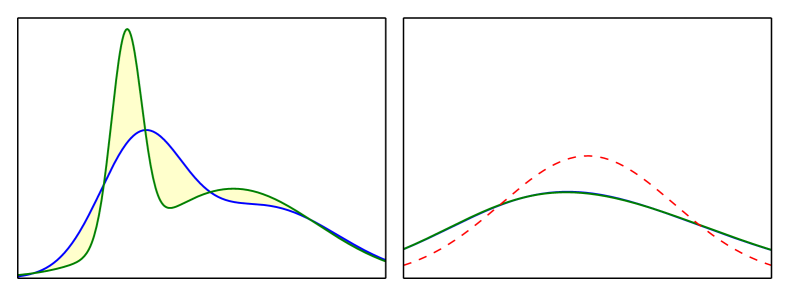
Figure 1: Mixtures with matching first $5$ moments before and after adding $N(0,2)$ (red).

Lemma 2.2.

Let $F$ and $G$ be distributions that are subgaussian with constant parameters and identical first $k$ moments for $k=O(1)$. Let $P=F+N(0,\sigma^{2})$ and $Q=G+N(0,\sigma^{2})$ for $\sigma\gtrsim 1$. Then

$$\mathrm{H}^{2}(P,Q)\lesssim 1/\sigma^{2k+2}.$$

Proof.

We have that $F$ and $G$ are subgaussian with constant parameters, i.e., for any $d\geq 0$ we have

$$\left|\operatorname*{\mathbb{E}}_{t\sim F}t^{d}\right|\lesssim(O(\sqrt{d}))^{d}$$

and similarly for $G$. Denote by $p,q,f,g$ density functions of $P,Q,F,G,$ respectively. We would like to bound

$$\mathrm{H}^{2}(P,Q)=\frac{1}{2}\int_{-\infty}^{\infty}\left(\sqrt{p(x)}-\sqrt{q(x)}\right)^{2}\mathrm{d}x\,.$$ (2)

We split the integral (2) into two regimes, $|x|\geq T$ and $|x|\leq T$ for $T\eqsim\sigma\sqrt{\log\sigma}$.

For the $|x|\geq T$ regime, we have

$$\frac{1}{2}\int_{|x|\geq T}\left(\sqrt{p(x)}-\sqrt{q(x)}\right)^{2}\mathrm{d}x \leq\operatorname*{\mathbb{P}}_{x\sim P}\left\{|x|\geq T\right\}+Pr_{x\sim Q}\left\{|x|\geq T\right\}$$

$$\lesssim e^{-T^{2}/(2(\sigma^{2}+O(1)))}$$

$$\lesssim 1/\sigma^{2k+2}\,.$$

The challenging part is the $|x|\leq T$ regime.

Claim 2.3.

For $|x|\leq T,$ we have

$$p(x)\gtrsim\frac{1}{\sqrt{2\pi}\sigma}e^{-x^{2}/(2\sigma^{2})}.$$ (3)

Proof.

Let $x$ be such that $|x|\leq T.$ Let $t$ be such that $F([-t,t])=1/2.$ Note that $t=O(1)$ since all the parameters of $F$ are constant. In particular, denoting by $\nu(y)$ the density of $N(0,\sigma^{2})$ we have for every $y\in[-t,t],$

$$\nu(x-y)\geq\frac{e^{-(|x|+t)^{2}/2\sigma^{2}}}{\sqrt{2\pi}\sigma}\geq\frac{e^{-x^{2}/2\sigma^{2}}e^{-O(|x|/\sigma^{2})}e^{-O(1/2\sigma^{2})}}{\sqrt{2\pi}\sigma}\gtrsim\frac{1}{\sqrt{2\pi}\sigma}e^{-x^{2}/(2\sigma^{2})}.$$

Hence,

$$p(x)\geq\int_{-t}^{t}f(x)\nu(x-y)\mathrm{d}y\geq\frac{1}{2}\cdot\min_{y\in[-t,t]}\nu(x-y)\gtrsim\frac{1}{2}\cdot\frac{1}{\sqrt{2\pi}\sigma}e^{-x^{2}/(2\sigma^{2})}\,.$$

∎

Now, we define

$$\Delta(x)=\frac{q(x)-p(x)}{p(x)}.$$

We have that

$$\Delta(x) =\frac{1}{p(x)}\int_{-\infty}^{\infty}\frac{1}{\sqrt{2\pi}\sigma}e^{-\frac{(x-t)^{2}}{2\sigma^{2}}}(g(t)-f(t))\mathrm{d}t$$

$$=\frac{1}{p(x)}\frac{1}{\sqrt{2\pi}\sigma}e^{-x^{2}/(2\sigma^{2})}\int_{-\infty}^{\infty}e^{tx/\sigma^{2}}e^{-\frac{t^{2}}{2\sigma^{2}}}(g(t)-f(t))\mathrm{d}t$$

$$\lesssim\int_{-\infty}^{\infty}e^{tx/\sigma^{2}}e^{-\frac{t^{2}}{2\sigma^{2}}}(g(t)-f(t))\mathrm{d}t.$$ (4)

We take a power series expansion of the interior of the integral,

$$e^{tx/\sigma^{2}}e^{-\frac{t^{2}}{2\sigma^{2}}} =\left(\sum_{d=0}^{\infty}\frac{(tx/\sigma^{2})^{d}}{d!}\right)\left(\sum_{d=0}^{\infty}\frac{(-t^{2}/(2\sigma^{2}))^{d}}{d!}\right)$$

$$=\sum_{d=0}^{\infty}\sum_{\begin{subarray}{c}j\in\mathbb{Z}\\ 0\leq 2j\leq d\end{subarray}}\frac{(tx/\sigma^{2})^{d-2j}}{(d-2j)!}\frac{(-t^{2}/(2\sigma^{2}))^{j}}{j!}$$

$$=\sum_{d=0}^{\infty}(t/\sigma)^{d}\sum_{\begin{subarray}{c}j\in\mathbb{Z}\\ 0\leq 2j\leq d\end{subarray}}\frac{(x/\sigma)^{d-2j}(-1/2)^{j}}{(d-2j)!j!}.$$

Now, for all $j\in[0,d/2]$,

$$(d-2j)!j!\geq(d/2-\sqrt{d})!=(\Omega(d))^{d/2-\sqrt{d}}=(\Omega(d))^{d/2}\,.$$

Therefore each term in the inner sum has magnitude bounded by $(x/\sigma)^{d-2j}(O(1/d))^{d/2}$, so the sum has magnitude bounded by $(1+(x/\sigma)^{d})(O(1/d))^{d/2}$. Hence there exists a constant $C$ and values $c_{x,d}$ with $|c_{x,d}|\leq 1$ such that

$$e^{tx/\sigma^{2}}e^{-\frac{t^{2}}{2\sigma^{2}}}=\sum_{d=0}^{\infty}c_{x,d}\left(\frac{C(1+x/\sigma)}{\sigma\sqrt{d}}\right)^{d}t^{d}.$$

Returning to (4), we have

$$\Delta(x) \lesssim\int_{-\infty}^{\infty}\sum_{d=0}^{\infty}c_{x,d}\left(\frac{C(1+x/\sigma)}{\sigma\sqrt{d}}\right)^{d}t^{d}(g(t)-f(t))\mathrm{d}t$$

$$=\sum_{d=0}^{\infty}c_{x,d}\left(\frac{C(1+x/\sigma)}{\sigma\sqrt{d}}\right)^{d}\int_{-\infty}^{\infty}t^{d}(g(t)-f(t))\mathrm{d}t$$

$$\leq\sum_{d=0}^{\infty}|c_{x,d}|\left(\frac{C(1+x/\sigma)}{\sigma\sqrt{d}}\right)^{d}\left\{\begin{array}[]{cl}0&\text{if }d\leq k\\ (O(\sqrt{d}))^{d}&\text{otherwise}.\end{array}\right.$$

$$\lesssim\sum_{d=k+1}^{\infty}\left(\frac{O(1)\cdot C(1+x/\sigma)}{\sigma}\right)^{d}$$

$$\eqsim\left(\frac{1+x/\sigma}{\sigma}\right)^{k+1}.$$

for all $|x|\leq T\eqsim\sigma\log\sigma$. Note that this implies $|\Delta(x)|<1$ which justifies the expansion

$$\sqrt{1+\Delta(x)}=1+\Delta(x)/2\pm O(\Delta(x)^{2}).$$

Therefore, following the approach outlined in [Pol00], we can write

$$\mathrm{H}^{2}(P,Q) =1-\int_{-\infty}^{\infty}\sqrt{p(x)q(x)}\mathrm{d}x$$

$$=1-O(1/\sigma^{2k+2})-\int_{-T}^{T}p(x)\sqrt{1+\Delta(x)}\mathrm{d}x$$

$$=1-O(1/\sigma^{2k+2})-\int_{-T}^{T}p(x)(1+\Delta(x)/2\pm O(\Delta(x)^{2}))\mathrm{d}x$$

Now, we have that

$$\int_{-T}^{T}p(x)\left(1+\frac{1}{2}\Delta(x)\right)\mathrm{d}x =\operatorname*{\mathbb{P}}_{x\sim P}[|x|\leq T]+\frac{1}{2}\left(\operatorname*{\mathbb{P}}_{x\sim Q}\left\{|x|\leq T\right\}-\operatorname*{\mathbb{P}}_{x\sim P}\left\{|x|\leq T]\right\}\right)$$

$$=1-\frac{1}{2}\left(\operatorname*{\mathbb{P}}_{x\sim Q}\left\{|x|>T\right\}+\operatorname*{\mathbb{P}}_{x\sim P}\left\{|x|>T\right\}\right)$$

$$=1-O(1/\sigma^{2k+2})$$

by our choice of $T.$ We conclude,

$$\mathrm{H}^{2}(P,Q) \lesssim 1/\sigma^{2k+2}+\int_{-T}^{T}p(x)\left(\frac{1+x/\sigma}{\sigma}\right)^{2k+2}\mathrm{d}x$$

$$\lesssim 1/\sigma^{2k+2}\left(1+\int_{-T}^{T}p(x)(x/\sigma)^{2k+2}\mathrm{d}x\right)$$

$$\leq 1/\sigma^{2k+2}\left(1+\operatorname*{\mathbb{E}}_{x\sim P}(x/\sigma)^{2k+2}\right)$$

$$\lesssim 1/\sigma^{2k+2}\,.$$

∎

2.2 Lower bounds for mixtures of two Gaussians

Claim 2.4.

Let $P$ and $Q$ be distributions with $\mathrm{H}^{2}(P,Q)\leq\epsilon$. Then there exists a constant $c>0$ such that $n=c\epsilon^{-1}\log(1/\delta)$ independent samples from $P$ and $Q$ have total variation distance less than $1-\delta.$ In particular, we cannot distinguish the distributions from $n$ samples with success probability greater than $1-\delta.$

Proof.

Let $x_{1},\dotsc,x_{n}\sim P$ and $y_{1},\dotsc,y_{n}\sim Q$ for $n=c\epsilon^{-1}\log(1/\delta)$. We will show that the total variation distance between $(x_{1},\dotsc,x_{n})$ and $(y_{1},\dotsc,y_{n})$ is less than $1-\delta$.

We partition $[n]$ into $k$ groups of size $1/(10\epsilon)$, for $k=10c\log(1/\delta)$. Within each group, by sub-additivity of squared Hellinger distance we have that

$$\mathrm{H}^{2}\big{(}(x_{1},\dotsc,x_{1/(10\epsilon)}),(y_{1},\dotsc,y_{1/(10\epsilon)})\big{)}\leq 1/10\,.$$

Appealing to the relation between total variation and Hellinger, this implies

$$\mathrm{TV}\big{(}(x_{1},\dotsc,x_{1/(10\epsilon)}),(y_{1},\dotsc,y_{1/(10\epsilon)})\big{)}\leq 2\mathrm{H}\big{(}(x_{1},\dotsc,x_{1/(10\epsilon)}),(y_{1},\dotsc,y_{1/(10\epsilon)})\big{)}\leq\frac{2}{3}\,.$$

Hence we may sample $(x_{1},\dotsc,x_{1/(10\epsilon)})$ and $(y_{1},\dotsc,y_{1/(10\epsilon)})$ in such a way that the two are identical with probability at least $1/3$. If we do this for all $k$ groups, we have that $(x_{1},\dotsc,x_{n})=(y_{1},\dotsc,y_{n})$ with probability at least $1/3^{k}>2\delta$ for sufficiently small constant $c$. ∎

Theorem 2.5.

Consider any algorithm that, given $n$ samples of any gaussian mixture with variance $\sigma^{2}$, with probability $1-\delta$ learns either $\mu_{i}$ to $\pm\epsilon\sigma$ or $\sigma_{i}^{2}$ to $\pm\epsilon^{2}\sigma^{2}$. Then $n=\Omega(\epsilon^{-12}\log(1/\delta))$.

Proof.

Take any two gaussian mixtures $F$ and $G$ with constant parameters such that the four means and variances are all $\Omega(1)$ different from each other, but $F$ and $G$ match in the first five moments. One can find such mixtures by taking almost any mixture $F$ with constant parameters and solving $p_{5}$ to find another root and the corresponding mixture (per Lemma B.1, this will cause the first five moments to match). We can find such an $F$ and $G$ in [Pea94], or alternatively take

$$F =\frac{1}{2}N(-1,1)+\frac{1}{2}N(1,2)$$

$$G \approx 0.2968N(-1.2257,0.6100)+0.7032N(0.5173,2.3960).$$ (5)

While $G$ is expressed numerically, one can certainly prove that the $p_{5}$ derived from $F$ has a second root that yields something close to this mixture. Plug the mixtures into Lemma 2.2. We get that for any $\sigma>0$, the mixtures

$$P =\frac{1}{2}N(-1,1+\sigma^{2})+\frac{1}{2}N(1,2+\sigma^{2})$$

$$Q \approx 0.2968N(-1.2257,0.6100+\sigma^{2})+0.7032N(0.5173,2.3960+\sigma^{2}).$$

have

$$\mathrm{H}^{2}(P,Q)\lesssim 1/\sigma^{12}.$$ (6)

Since by Claim 2.4 we cannot differentiate $P$ and $Q$ with $o(\sigma^{12}\log(1/\delta))$ samples, it requires $\Omega(\sigma^{12}\log(1/\delta))$ samples to learn either the $\mu_{i}$ or the $\sigma_{i}^{2}$ to $\pm 1/10$ with $1-\delta$ probability. Set $\sigma=1/(10\epsilon)$ to get the result. ∎

Our argument extends to $d$ dimensions. We gain a $\log(d)$ factor in our lower bound by randomly planting a hard mixture learning problem in each of the $d$ coordinates.

Claim 2.6.

Let $P$ and $Q$ be distributions with $\mathrm{H}^{2}(P,Q)\leq\epsilon$. Let $R_{i}\in\{P,Q\}$ uniformly at random for $i\in\{1,\dots,d\}$. Then there exists a constant $c>0$ such that given $n=c\epsilon^{-1}\log(d/\delta)$ no algorithm can identify all $R_{i}$ with probability $1-\delta.$

Proof.

As in Claim 2.4, we have that the total variation distance between $B=1/(10\epsilon)$ samples from $P$ and $B$ samples from $Q$ is less than $2/3$.

Partition our samples into $k=10c\log d$ groups $x^{1},\dotsc,x^{k}$, where for each group $j\in[k]$ and coordinate $i\in[d]$ we have $x^{j}_{i}\sim R_{i}^{\otimes B}$. By the total variation bound between $P^{\otimes B}$ and $Q^{\otimes B}$, we could instead draw $x^{j}_{i}$ from a distribution independent of $R_{i}$ with probability $1/3$ and a distribution dependent on $R_{i}$ with probability $2/3$. Suppose we do this.

Then for any coordinate $i$, with probability $3^{-k}>\delta/d$ all of $x^{1}_{i},\dotsc,x^{k}_{i}$ are independent of $R_{i}$. Since the coordinates are independent, this means that with probability at least

$$1-(1-\delta/d)^{d}\geq\delta/4$$

there will exist a coordinate $i$ such that all of $x^{1}_{i},\dotsc,x^{k}_{i}$ are independent of $R_{i}$. The algorithm must then guess $R_{i}$ incorrectly with probability at least $1/2$, for a $\delta/8$ probability of failure overall. Rescale $\delta$ to get the result. ∎

This immediately gives that Theorem 2.5 can be extended to $d$ dimensions:

Theorem 2.7.

Consider any algorithm that, given $n$ samples of any $d$-dimensional gaussian mixture $F$ with $\operatorname*{\mathbb{V}}(F)=\sigma^{2}$, with probability $1-\delta$ for all $i\in[d]$ learns either $\mu_{i}$ to $\pm\epsilon\sigma$ or $\Sigma_{i,i}$ to $\pm\epsilon^{2}\sigma^{2}$. Then $n=\Omega(\epsilon^{-12}\log(d/\delta))$.

Proof.

Let $P,Q$ be as in Theorem 2.5. We choose a mixture $F$ to have independent coordinates, each of which is uniformly chosen from $\{P,Q\}$. Then $\operatorname*{\mathbb{V}}(F)\eqsim 1/\epsilon$, $H(P,Q)\leq\epsilon^{6}$, and learning the parameters of the mixture in the $i$th coordinate to the specified precision would identify whether it is $P$ or $Q$. Claim 2.6 gives the result. ∎

2.3 Lower bound for mixtures of $k$ gaussians

We can extend these lower bounds to mixtures of $k$ gaussians. The main issue is that for $k=2$ we know that two explicit well-separated mixtures exist that match on $5$ moments, by solving the method of moments on a random input and getting two solutions. For general $k$ we would like to show the existence of two well-separated mixtures that match on nearly $3k$ moments.

We will formalize the following intuition. With $k$ gaussians there are $3k-1$ free parameters– means, variances, and probabilities subject to the probabilities summing to one. Therefore if we only take $3k-2$ moments, we are embedding a high dimensional space into a lower dimensional space, and expect lots of collisions. Therefore some pair that collide should be well separated.

First we show a few lemmas that will be useful. We use the following fact, shown in the appendix:

Lemma A.8.

Let $p(x)=p(x_{1},\dotsc,x_{n})$ be a multivariate polynomial of degree $d$ and smallest nonzero coefficient of magnitude $a$. Then

$$\operatorname*{\mathbb{P}}_{x\sim N(0,I_{n})}[|p(x)|<a\epsilon]<d\epsilon^{1/d}.$$

This lets us show the following:

Lemma 2.8.

Let $k\geq 1$ be a constant. There exists a set of $k$ gaussians $N(\mu_{i},\sigma_{i}^{2})$ such that all the $\mu_{i}$ and $\sigma_{i}$ are $O(1)$, all $\mu_{i}$ and $\sigma_{i}$ are $\Omega(1)$ far from the others and from zero, and the matrix $A\in\mathbb{R}^{m\times k}$ of moments, given by

$$A_{j,i}=\operatorname*{\mathbb{E}}_{x\sim N(\mu_{i},\sigma_{i}^{2})}x^{j},$$

has minimum singular value $\Omega(1)$ for any $m\geq k$.

Proof.

We will show this to be true with good probability for a randomly drawn set of $k$ gaussians. We consider drawing the gaussians randomly, so $\mu_{i}\sim N(0,1)$ and $\sigma_{i}\sim N(0,1)^{2}$. This immediately gives the first two properties with probability arbitrarily close to $1$, and we just need to bound the minimum singular value of $A$. We can assume without loss of generality that $m=k$, since this minimizes the singular values. Then, since $A$ has $O(1)$ dimension and coefficients, it suffices to show that the determinant of $A$—which is the product of the eigenvalues—is $\Omega(1)$ with positive probability.

Now, consider the determinant of $A$ as a formal polynomial in the $\mu_{i}$ and $\sqrt{\sigma_{i}}$. We know that this is nonzero, because (for example) the $\mu_{1}^{1}\mu_{2}^{2}\mu_{3}^{3}\dotsb\mu_{k}^{k}$ monomial appears only from the diagonal term. It is a fixed monomial, so its minimum coefficient is some constant. Hence Lemma A.8 shows for $\mu_{i},\sqrt{\sigma_{i}}\sim N(0,1)$ that the determinant will be $\Omega(1)$ with probability arbitrarily close to $1$. In such cases, the minimum singular value is $\Omega(1)$ as well, giving the result. ∎

Lemma 2.9.

Let $k\geq 1$ be a constant. There exist two mixtures $F$ and $G$ of $k$ gaussians each that match on the first $3k-2$ moments, for which all the parameters $(p_{i},\mu_{i},\sigma_{i})$ are bounded by $O(1)$ for each mixture, and for which one of the mixtures has either a $\mu_{i}$ or a $\sigma_{i}$ that is $\Omega(1)$ far from any $\mu_{i}$ or $\sigma_{i}$ in the other mixture.

Proof.

There are $t=3k-1$ “free” parameters in a mixture of $k$ gaussians: the means, variances, and relative probabilities subject to the sum of probabilities equalling $1$. With $t$ parameters, we expect there to be lots of mixtures that match on $t-1$ moments.

Formally, consider the $(\mu_{i},\sigma_{i})$ given by Lemma 2.8. For the matrix of moments $A$ as given by the lemma, and for any vector $p\in\mathbb{R}^{k}$ of probabilities for each gaussian, the first $m$ moments of the mixture $(p_{i},\mu_{i},\sigma_{i})$ are precisely $Ap$. Let $p_{i}=1/k$ for all $i$.

Now, let $0<\alpha<\beta\leq\frac{1}{k^{2}}$ be small constants to be determined later. For any set of free parameters $z\in\mathbb{R}^{t}$, consider a mixture of gaussians $f(z)=\{(p^{\prime}_{i},\mu^{\prime}_{i},\sigma^{\prime}_{i})\}$ given by $\mu^{\prime}_{i}=\mu_{i}+\alpha z_{i}$, $\sigma^{\prime}_{i}=\sigma_{i}+\alpha z_{k+i}$, and $p^{\prime}_{i}=p_{i}+\beta z_{2k+i}$ for $i\in[k-1]$ and $p^{\prime}_{k}=p_{k}-\sum_{i\in[k-1]}\beta z_{2k+i}$. For every $z$ with $\lVert z\rVert_{2}=1$, this is a valid mixture of $k$ gaussians (because $\beta$ is small enough that $\sum_{i\in[k-1]}\beta z_{2k+i}<p_{k}$). For such a $z$, define $A(z)\in\mathbb{R}^{m\times k}$ to be the matrix of component moments, $A(z)_{j,i}=\operatorname*{\mathbb{E}}_{x\sim N(\mu^{\prime}_{i},\sigma^{\prime}_{i})}x^{j}$, and $p(z)\in\mathbb{R}^{k}$ to be the vector of probabilities $p^{\prime}$. Then the first $m$ moments of the mixture $f(z)$ are $M(z)=A(z)p(z)$.

Note that, for any $\alpha,\lVert z\rVert\leq 1$, we have $\lVert A(z)-A(0)\rVert\lesssim\alpha\lVert z\rVert$: every monomial in the matrix $A(z)-A(0)$ includes $\alpha$ times a coordinate of $z$ in it, and there are only a constant number of monomials.

Because $M(z)$ is a polynomial in $z$, it is continuous. If $m=t-1=3k-2$, then the Borsuk-Ulam theorem states that there exist two antipodal points $z,-z$ with $\lVert z\rVert_{2}=1$ such that $M(z)=M(-z)$. This immediately gives two different mixtures that match on the first $m$ moments. This is almost what we want, but we also need the mixtures to be different over $\sigma$ or $\mu$, not just $p$.

We have that $A(z)p(z)=A(-z)p(-z)$, or

$$A(0)(p(z)-p(-z))=(A(-z)-A(0))p(-z)-(A(z)-A(0))p(z)$$

For $\sigma_{min}=\Omega(1)$ being the minimal singular value of $A(0)$, we have

$$\sigma_{min}\lVert p(z)-p(-z)\rVert_{2} \leq\lVert A(0)(p(z)-p(-z))\rVert=\lVert(A(-z)-A(0))p(-z)-(A(z)-A(0))p(z)\rVert$$

$$\lVert p(z)-p(-z)\rVert_{2} \leq\frac{1}{\sigma_{min}}(\lVert A(-z)-A(0)\rVert+\lVert A(z)-A(0)\rVert)(\lVert p(-z)\rVert+\lVert p(z)\rVert)$$

$$\leq\frac{1}{\Omega(1)}\cdot O(\alpha)\cdot 2\lesssim\alpha.$$

On the other hand, $\lVert p(z)-p(-z)\rVert_{2}\geq\beta\sqrt{\sum_{i>2k}z_{i}^{2}}$, so

$$\sqrt{\sum_{i>2k}z_{i}^{2}}\lesssim\frac{\alpha}{\beta}.$$

If we set $\beta$ to some value (e.g. $1/k^{2}$), then if we choose $\alpha$ as a small enough constant we will have $\sqrt{\sum_{i>2k}z_{i}^{2}}\leq 1/2$. Since $\lVert z\rVert_{2}=1$, this means $\sqrt{\sum_{i\leq 2k}z_{i}^{2}}\geq\sqrt{3/4}\gtrsim 1$. Therefore the mixtures $f(z)$ and $f(-z)$ have at least one of their $\mu_{i}$ or $\sigma_{i}$ perturbed by $\Theta(\alpha)$. For small enough constant $\alpha$, the perturbations will be much less than the $\Omega(1)$ gap between all the different $\mu_{i}$ and $\sigma_{i}$ in the mixture $f(0)$. Therefore the perturbed $\mu_{i}$ or $\sigma_{i}$ in $f(z)$ is $\Omega(1)$ far from any corresponding $\mu_{i}$ or $\sigma_{i}$ in $f(-z)$. So $f(z)$ and $f(-z)$ give the desired mixtures. ∎

The mixtures given by Lemma 2.9 let us extend the lower bounds to mixtures of $k$ gaussians, but with a caveat: the mixtures differ in at least one of $\mu_{i}$ and $\sigma_{i}$, so the lower bound now only applies to algorithms that recover both $\mu_{i}$ and $\sigma_{i}$ do the desired precision.

Theorem 2.10.

Consider any algorithm that, given $n$ samples of any one dimensional gaussian mixture $F$ of $k=O(1)$ components, with probability $1-\delta$ learns both the $\mu_{i}$ to $\pm\epsilon\sigma$ and the $\sigma_{i}^{2}$ to $\pm\epsilon^{2}\sigma^{2}$. Then $n=\Omega_{k}(\epsilon^{2-6k}\log(1/\delta))$.

Theorem 2.11.

Consider any algorithm that, given $n$ samples of any $d$-dimensional gaussian mixture $F$ of $k=O(1)$ components with $\operatorname*{\mathbb{V}}(F)=\sigma^{2}$, with probability $1-\delta$ for all $i\in[d]$ learns both $\mu_{i}$ to $\pm\epsilon\sigma$ and $\Sigma_{i,i}$ to $\pm\epsilon^{2}\sigma^{2}$. Then $n=\Omega_{k}(\epsilon^{2-6k}\log(d/\delta))$.

Proof.

Identical to the proof of Theorems 2.5 and 2.7, but applying Lemma 2.2 to the $F$, $G$ resulting from Lemma 2.9 rather than the explicit ones in Equation (5). ∎

3 Algorithm for one-dimensional mixtures

3.1 Preliminaries and Notation

Asymptotics.

For any expressions $f$ and $g$, we use $f\lesssim g$ to denote that there exists a constant $C>0$ such that $f\leq Cg$. Similarly, $f\gtrsim g$ denotes that $g\lesssim f$, and $f\eqsim g$ denotes that $f\lesssim g\lesssim f$.

Parameters of the gaussian.

The two gaussians have probabilities $p_{i}$, means $\mu_{i}$, and standard deviations $\sigma_{i}$. The overall mean and variance of the mixture are $\mu=p_{1}\mu_{1}+p_{2}\mu_{2}$ and

$$\sigma^{2}=p_{1}((\mu_{1}-\mu)^{2}+\sigma_{1}^{2})+p_{2}((\mu_{2}-\mu)^{2}+\sigma_{2}^{2})=p_{1}p_{2}(\mu_{1}-\mu_{2})^{2}+p_{1}\sigma_{1}^{2}+p_{2}\sigma_{2}^{2}\,.$$ (7)

For almost all of the section, for simplicity of notation we will assume that the overall mean $\mu=0$. We only need to consider $\mu\neq 0$ when showing that we can estimate the moments precisely enough.

We will also assume that $p_{1},p_{2}\in(0,1)$ are both bounded away from zero. We define

$$\Delta_{\mu}=|\mu_{2}-\mu_{1}|\qquad\Delta_{\sigma^{2}}=|\sigma_{2}^{2}-\sigma_{1}^{2}|\,.$$ (8)

We also make use of a reparameterization of the gaussian distribution:

$$\alpha=-\mu_{1}\mu_{2}\qquad\beta=\mu_{1}+\mu_{2}\qquad\gamma=\frac{\sigma_{2}^{2}-\sigma_{1}^{2}}{\mu_{2}-\mu_{1}}$$ (9)

Note that these are independent of adding gaussian noise, i.e. increasing both $\sigma_{1}^{2}$ and $\sigma_{2}^{2}$ by the same amount. Also we have $\alpha\geq 0$, since the mean is zero. With our assumption that $p_{1},p_{2}$ are bounded away from zero we have that

$$\beta^{2}\lesssim\alpha\eqsim\Delta_{\mu}^{2}.$$

Finally, we will make use of the parameter

$$\kappa=\max(1,\Delta_{\sigma^{2}}/\Delta_{\mu}^{2})$$

which will relate to how well-conditioned our equations are. We have that $|\gamma|\lesssim\Delta_{\mu}\kappa$.

Excess moments.

We define $M_{i}$ to be the $i$th moment of our distribution, $\operatorname*{\mathbb{E}}[x^{i}]$, so $M_{2}=\sigma^{2}$.

The excess kurtosis of a distribution is a standard statistical measure defined as $M_{4}/M_{2}^{2}-3$. It is designed to be independent of adding independent gaussian noise to the variable. Inspired by this, we define the excess moments $X_{i}$ to be $M_{i}$ plus a polynomial in $M_{2},\dotsc,M_{i-1}$ such that the result is independent of adding gaussian noise. We have that:

Lemma 3.1.

For $\alpha=-\mu_{1}\mu_{2},\beta=\mu_{1}+\mu_{2},\gamma=\frac{\sigma_{2}^{2}-\sigma_{1}^{2}}{\mu_{2}-\mu_{1}}$ we have that

$$X_{3} :=M_{3} =\alpha\beta+3\alpha\gamma$$

$$X_{4} :=M_{4}-3M_{2}^{2} =-2\alpha^{2}+\alpha\beta^{2}+6\alpha\beta\gamma+3\alpha\gamma^{2}$$ (10)

$$\ X_{5} :=M_{5}-10M_{3}M_{2} =\alpha(\beta^{3}-8\alpha\beta+10\beta^{2}\gamma+15\gamma^{2}\beta-20\alpha\gamma)$$

$$X_{6} :=M_{6}-15M_{4}M_{2}+30M_{2}^{3} =\alpha(16\alpha^{2}-12\alpha\beta^{2}-60\alpha\beta\gamma+\beta^{4}+15\beta^{3}\gamma+45\beta^{2}\gamma^{2}+15\beta\gamma^{3})$$

See Appendix B.2 for proof. Since $\alpha,\beta,\gamma$ are independent of adding gaussian noise, these definitions of the $X_{i}$ are correct.

By inspection, we have for each $i\in\{3,4,5,6\}$ that

$$|X_{i}|\lesssim\Delta_{\mu}^{i}\kappa^{i-2}.$$ (11)

For simplicity of notation, we also define $X_{1}=\mu$ and $X_{2}=\sigma^{2}$, despite them not technically being “excess,” and refer to $\{X_{1},X_{2},X_{3},X_{4},X_{5},X_{6}\}$ as the excess moments.

Estimation of moments.

All our algorithms in this section proceed by first estimating the (excess) moments from the samples, then estimating the mixture from these moments. The relationship between sample complexity and estimation error is as follows:

Lemma 3.2.

Suppose $p_{1},p_{2}$ are bounded away from zero and our mixture has variance $\sigma^{2}$. Given $O(\log(1/\delta)/\epsilon^{2})$ samples, with probability $1-\delta$ we can compute estimates $\widehat{X}_{i}$ of the first $O(1)$ excess moments $X_{i}$ satisfying $|\widehat{X}_{i}-X_{i}|\leq\epsilon\sigma^{i}$ .

See Appendix A.2 for a proof. We will state our first two theorems in terms of the necessary error bound on $|\widehat{X}_{i}-X_{i}|$ rather than sample complexity. This is more general, since it supports other forms of perturbation of the inputs.

For a statistic $f$ of the gaussian mixture, in general we use $f$ to denote the true value of the statistic and $\widehat{f}$ to denote the estimate of $f$ from estimates of the moments.

3.2 Algorithm overview

Our overall goal is to recover the $\mu_{i}$ to $\pm\epsilon\sigma$ and the $\sigma_{i}^{2}$ to $\pm\epsilon^{2}\sigma^{2}$ using roughly $O(1/\epsilon^{12})$ samples.

We have two different algorithms for different parameter regimes. The first algorithm, Algorithm 1, proceeds by first learning the $\mu_{i}$, then using this to estimate the $\sigma_{i}$. However, it only works well if we have the $X_{i}$ to within $\Delta_{\mu}^{i}$; without this, we cannot get a nontrivial estimate of the $\mu_{i}$, which causes the algorithm to also not get a decent estimate of the $\sigma_{i}$.

Theorem 3.7 (Precision better than $\Delta_{\mu}$).

Consider any mixture of gaussians where $p_{1}$ and $p_{2}$ are bounded away from zero, $c>0$ a sufficiently small constant, and any $\epsilon<1$. If $|\widehat{X}_{i}-X_{i}|\leq c\epsilon\Delta_{\mu}^{i}$ for all $i\leq 6$, Algorithm 1 recovers the $p_{i}$ to $\pm\epsilon$, $\mu_{i}$ to $\pm\epsilon\Delta_{\mu}$, and $\sigma_{i}^{2}$ to $\pm\epsilon\Delta_{\mu}^{2}$.

If $\Delta_{\sigma^{2}}\gg\Delta_{\mu}^{2}$, for example if $\Delta_{\mu}=0$, one may hope to get a good estimate of the $\sigma_{i}^{2}$ despite having more than $\Delta_{\mu}^{i}$ error in $X_{i}$. Algorithm 2 does this by solving for the $\sigma_{i}$ under the assumption that $\mu_{1}=\mu_{2}$. We can show that the solution is robust to $\Delta_{\mu}$ being small but nonzero, so the algorithm does a good job when $\Delta_{\mu}^{i}\lesssim|\widehat{X}_{i}-X_{i}|\lesssim\Delta_{\sigma^{2}}^{i/2}$. (When $|\widehat{X}_{i}-X_{i}|$ goes below this bound, the performance doesn’t degrade but does not improve as one would like.)

Theorem 3.9 (Precision between $\Delta_{\mu}$ and $\sqrt{\Delta}_{\sigma^{2}}$).

Consider any mixture of gaussians where $p_{1}$ and $p_{2}$ are bounded away from zero, and any $\epsilon<1$. Suppose that $\epsilon\Delta_{\sigma^{2}}\gtrsim\Delta_{\mu}^{2}$. If $|\widehat{X}_{i}-X_{i}|\leq\epsilon\Delta_{\sigma^{2}}^{i/2}$ for all $i\leq 6$, Algorithm 2 recovers the $p_{i}$ to $\pm O(\epsilon)$ and $\sigma_{i}^{2}$ to $\pm O(\epsilon)\Delta_{\sigma^{2}}$.

In the remaining parameter regime, with $|\widehat{X}_{i}-X_{i}|>\Delta_{\mu}^{i}+\Delta_{\sigma^{2}}^{i/2}$, the two gaussians are in general indistinguishable and it suffices to just output the average mean and variance.

To get a general result, we just need to figure out which of the three parameter regimes we’re in and apply the appropriate algorithm. Algorithm 3 does this by constructing sufficiently good estimates of $\sigma,\Delta_{\mu},$ and $\Delta_{\sigma^{2}}$. We also invoke Lemma 3.2 to get bounds on sample complexity, showing:

Theorem 3.10.

Let $F$ be any mixture of two gaussians with variance $\sigma^{2}$ and $p_{1},p_{2}$ bounded away from $0.$ Then, given $O(\epsilon^{-2}n\log(1/\delta))$ samples Algorithm 3 with probability $1-\delta$ outputs the parameters of a mixture $\widehat{F}$ so that for some permutation $\pi$ and all $i\in\{1,2\}$ we have the following guarantees:

• If $n\geq\big{(}\frac{\sigma^{2}}{|\mu_{1}-\mu_{2}|^{2}}\big{)}^{6}$, then $|\mu_{i}-\widehat{\mu}_{\pi(i)}|\leq\epsilon|\mu_{1}-\mu_{2}|$, $|\sigma_{i}^{2}-\widehat{\sigma}_{\pi(i)}^{2}|\leq\epsilon|\mu_{1}-\mu_{2}|^{2}$, and $|p_{i}-\widehat{p}_{\pi(i)}|\leq\epsilon$.

• If $n\geq\big{(}\frac{\sigma^{2}}{|\sigma_{1}^{2}-\sigma_{2}^{2}|}\big{)}^{6}$, then $|\sigma_{i}^{2}-\widehat{\sigma}_{\pi(i)}^{2}|\leq\epsilon|\sigma_{1}^{2}-\sigma_{2}^{2}|+|\mu_{1}-\mu_{2}|^{2}$ and $|p_{i}-\widehat{p}_{\pi(i)}|\leq\epsilon+\frac{|\mu_{1}-\mu_{2}|^{2}}{|\sigma_{1}^{2}-\sigma_{2}^{2}|}$.

• For any $n\geq 1$, the algorithm performs as well as assuming the mixture is a single gaussian: $|\mu_{i}-\widehat{\mu}_{\pi(i)}|\leq|\mu_{1}-\mu_{2}|+\epsilon\sigma$ and $|\sigma_{i}^{2}-\widehat{\sigma}_{\pi(i)}^{2}|\leq|\sigma_{1}^{2}-\sigma_{2}^{2}|+|\mu_{1}-\mu_{2}|^{2}+\epsilon\sigma^{2}.$

The regimes can be unified to get the following, simpler but weaker, corollary:

Corollary 3.3.

Consider any mixture of gaussians where $p_{1}$ and $p_{2}$ are bounded away from zero, and any $\epsilon,\delta<1$. With $n=O(\log(1/\delta)/\epsilon^{12})$ samples, Algorithm 3 returns $\{\mu_{1},\mu_{2}\}$ to $\pm\epsilon\sigma$ additive error and the corresponding $\{\sigma_{1}^{2},\sigma_{2}^{2}\}$ to $\pm\epsilon^{2}\sigma^{2}$ additive error with probability $1-\delta$.

Proof.

If $\epsilon\sigma=f\Delta_{\mu}$ for $f<1$, then by the first clause of Theorem 3.10 with $\epsilon^{\prime}=f^{6}$ we get the $\mu_{i}$ to within $f^{6}\Delta_{\mu}\leq f\Delta_{\mu}=\epsilon\sigma$ and the $\sigma_{i}^{2}$ to within $f^{6}\Delta_{\mu}^{2}\leq f^{2}\Delta_{\mu}^{2}=\epsilon^{2}\sigma^{2}$.

Otherwise, if $\epsilon\sigma>\Delta_{\mu}$ but $\epsilon^{2}\sigma^{2}=f^{2}\Delta_{\sigma^{2}}$ for $f^{2}<1$, then by the second clause of Theorem 3.10 with $\epsilon^{\prime}=f^{6}$ we get the $\sigma_{i}$ to within $f^{6}\Delta_{\sigma^{2}}+\Delta_{\mu}^{2}\lesssim\epsilon^{2}\sigma^{2}$.

And by the last clause, if $\epsilon\sigma\gtrsim\Delta_{\mu}$ we get the $\mu_{i}$ to within $\Delta_{\mu}+\epsilon^{6}\sigma\lesssim\epsilon\sigma$, and if $\epsilon^{2}\sigma^{2}\gtrsim\max(\Delta_{\sigma^{2}},\Delta_{\mu}^{2})$ we get the $\sigma_{i}^{2}$ to within $\Delta_{\mu}^{2}+\Delta_{\sigma^{2}}+\epsilon^{6}\sigma^{2}\lesssim\epsilon^{2}\sigma^{2}$. ∎

3.3 Algorithm for better precision than $\Delta_{\mu}$

$\triangleright$ Recover gaussian mixture from (estimates of the) mean, variance, and excess moments

$\triangleright$ Excess moments are function of moments, defined in (10)

procedure RecoverFromMoments($\epsilon,\mu,\sigma^{2},X_{3},X_{4},X_{5},X_{6}$)

     $\alpha\leftarrow\textsc{RecoverAlphaFromMoments}(X_{3},X_{4},X_{5},X_{6},\epsilon)$.

     $\gamma\leftarrow\frac{1}{\alpha}\frac{\alpha^{2}X_{5}+2X_{3}^{3}+2\alpha^{3}X_{3}-3X_{3}X_{4}\alpha}{4X_{3}^{2}-2\alpha^{3}-3X_{4}\alpha}.$

     $\beta\leftarrow\frac{1}{\alpha}(X_{3}-3\alpha\gamma)$.

     $\mu_{1},\mu_{2}\leftarrow\frac{-\beta\mp\sqrt{\beta^{2}+4\alpha}}{2}$.

     $p_{1},p_{2}\leftarrow\frac{\mu_{2}}{\mu_{2}-\mu_{1}},\frac{-\mu_{1}}{\mu_{2}-\mu_{1}}$.

     $\sigma_{1}^{2}\leftarrow\sigma^{2}-\left(p_{1}\mu_{1}^{2}+p_{2}\mu_{2}^{2}-\mu_{1}\gamma\right)$.

     $\sigma_{2}^{2}\leftarrow\sigma_{1}^{2}+(\mu_{2}-\mu_{1})\gamma$.

     return $(p_{1},\mu_{1}+\mu,\sigma_{1}),(p_{2},\mu_{2}+\mu,\sigma_{2})$

end procedure

procedure RecoverAlphaFromMoments($X_{3},X_{4},X_{5},X_{6},\epsilon$)

     Let $y_{max}$ be the largest root of $2y^{3}+X_{4}y-X_{3}^{2}=0$.

     $\kappa\leftarrow 1+\sqrt{|X_{4}|}/y_{max}$ $\triangleright$ $\kappa=\Theta(1+|\gamma|/\sqrt{\alpha})$

     Define the $18$th degree polynomial $r(y)=p_{5}(y)^{2}+p_{6}(y)^{2}$ for $p_{5}$ and $p_{6}$ given by (14) and (3.3).

     $\triangleright$ For the true moments, $\alpha$ is the only zero of $r$ on $(0,y_{max}]$.

     Compute the set of roots $R$ of $r^{\prime}(y)$.

     Let $\alpha$ be maximal element of $R\cup\{(1+\epsilon/\kappa)y_{max}\}$ satisfying

$$\alpha \leq(1+\epsilon/\kappa)y_{max}$$

$$r(\alpha) \leq\epsilon^{2}\alpha^{18}\kappa^{10}.$$

     return $\alpha$.

end procedure

Algorithm 1 Algorithm for recovery of mixture of two gaussians in one dimension when the means are separated.

In this section we derive Pearson’s polynomial and extend it into a robust algorithm.

Manipulation of $X_{3},X_{4},X_{5}$.

Based on (10) we can remove $\beta$ to get an equation in $\{\alpha,\gamma,X_{3},X_{4}\}$:

$$6(\alpha\gamma)^{2} =X_{3}^{2}-2\alpha^{3}-X_{4}\alpha.$$ (12)

If we define $z:=\alpha\gamma$, we can get another equation in $\{\alpha,z,X_{3},X_{4},X_{5}\}$.

$$\alpha^{2}X_{5}-X_{3}^{3}+8\alpha^{3}X_{3} =\alpha^{3}\beta^{2}\gamma-12\alpha^{3}\gamma^{2}\beta+4\alpha^{4}\gamma-27\alpha^{3}\gamma^{3}$$

$$=z(X_{3}-3z)^{2}-12z^{2}(X_{3}-3z)+4\alpha^{3}z-27z^{3}$$

$$=18z^{3}-18X_{3}z^{2}+(4\alpha^{3}+X_{3}^{2})z$$

Substituting in (12) we make the equation linear in $z$:

$$\alpha^{2}X_{5}-X_{3}^{3}+8\alpha^{3}X_{3} =3(z-X_{3})(X_{3}^{2}-2\alpha^{3}-X_{4}\alpha)+(4\alpha^{3}+X_{3}^{2})z$$

$$=(4X_{3}^{2}-2\alpha^{3}-3X_{4}\alpha)z+(3X_{3}X_{4}\alpha+6\alpha^{3}X_{3}-3X_{3}^{3})$$

or

$$z:=\alpha\gamma =\frac{\alpha^{2}X_{5}+2X_{3}^{3}+2\alpha^{3}X_{3}-3X_{3}X_{4}\alpha}{4X_{3}^{2}-2\alpha^{3}-3X_{4}\alpha}.$$ (13)

We can substitute $z$ back into (12) and clear the denominator to get a polynomial equation in the single variable $\alpha$:

$$p_{5}(\alpha)=6(2X_{3}\alpha^{3}+X_{5}\alpha^{2}-3X_{3}X_{4}\alpha+2X_{3}^{3})^{2}+(2\alpha^{3}+3X_{4}\alpha-4X_{3}^{2})^{2}(2\alpha^{3}+X_{4}\alpha-X_{3}^{2}) =0.$$ (14)

Therefore, given the excess moments $X_{i}$, we can find a set of candidate $\alpha$ by solving for the positive roots of $p_{5}(y)=0$. Unfortunately, there are in general multiple such roots. In fact, the first five moments do not suffice to uniquely identify a gaussian mixture, so we must incorporate the sixth moment.

Using the 6th moment.

Analogously to the creation of (13), we take the expression for $X_{6}$ in (10), replace $\beta$ with $X_{4}/\alpha-3\gamma$, then remove $\gamma^{2}$ terms using (12) to get

$$z:=\alpha\gamma=\frac{4X_{3}^{4}-4X_{3}^{2}X_{4}\alpha-8X_{3}^{2}\alpha^{3}-X_{4}^{2}\alpha^{2}+8X_{4}\alpha^{4}+X_{6}\alpha^{3}+4\alpha^{6}}{10X_{3}^{3}-7X_{3}X_{4}\alpha-2X_{3}\alpha^{3}}$$ (15)

(See Appendix B.3 for a more detailed explanation.) Combining with (13) and clearing the denominators gives that

$$p_{6}(\alpha) =(4X_{3}^{2}-3X_{4}\alpha-2\alpha^{3})(4X_{3}^{4}-4X_{3}^{2}X_{4}\alpha-8X_{3}^{2}\alpha^{3}-X_{4}^{2}\alpha^{2}+8X_{4}\alpha^{4}+X_{6}\alpha^{3}+4\alpha^{6})-{}$$

$$\qquad(10X_{3}^{3}-7X_{3}X_{4}\alpha-2X_{3}\alpha^{3})(2X_{3}^{3}-3X_{3}X_{4}\alpha+2X_{3}\alpha^{3}+X_{5}\alpha^{2})=0$$ (16)

which is another $9$th degree equation in $\alpha$ in terms of the excess moments.

We would like to say that $\alpha$ is the only common positive root of $p_{5}$ and $p_{6}$, but this is not always true. Fortunately, we can exclude the other common roots if we enforce an upper bound on $\alpha$.

Restricting the domain.

Let $y_{max}$ be the positive root of

$$2y^{3}+X_{4}y-X_{3}^{2}=0.$$ (17)

There is at most one such root by Descartes’ rule of signs. There exists such a root because if $X_{3}=\alpha(\beta+3\gamma)$ is zero, then $X_{4}=\alpha(\beta+3\gamma)^{2}-6\alpha\gamma^{2}-2\alpha^{2}$ is negative. And by (12), $\alpha\leq y_{max}$.

Moreover,

$$y_{max}\lesssim\alpha.$$ (18)

(Since $p_{1}$ and $p_{2}$ are bounded away from zero, $\beta^{2}\lesssim\alpha$. Then if $\gamma^{2}\lesssim\alpha$, this follows from a cubic polynomial with bounded coefficients having bounded roots. Otherwise, $X_{3}^{2}=\Theta(\alpha^{2}\gamma^{2})$ and $X_{4}=\Theta(\alpha\gamma^{2})$ are positive so $y_{max}\leq X_{3}^{2}/X_{4}\lesssim\alpha$.)

Combining the equations.

We will show that $y=\alpha$ is the only solution to the set of equations $0<y\leq y_{max},p_{5}(y)=0,p_{6}(y)=0$. This statement would suffice to recover the mixture given the exact excess moments, but we also want the algorithm to have robustness to small perturbations in the $X_{i}$. We therefore define

$$r(y):=p_{5}(y)^{2}+p_{6}(y)^{2},$$ (19)

which we know is zero at $\alpha$. We will show it is significantly non-zero for any candidate $y$ that is far from $\alpha$ and still within $[cy_{max},y_{max}]$ for any constant $c>0$.

The robustness will depend on the parameter

$$\kappa:=\max(1,\Delta_{\sigma^{2}}/\Delta_{\mu}^{2})\eqsim 1+|\gamma|/\sqrt{\alpha}.$$ (20)

This is intuitive because the excess moments $X_{i}$ are bounded by $O(\Delta_{\mu}^{i}\kappa^{i-2})$, which implies by inspection of (14) and (3.3) that for all $|y|\lesssim y_{max}$, every monomial in $p_{5}$ and $p_{6}$ has magnitude bounded by

$$O(\Delta_{\mu}^{18}\kappa^{6}).$$ (21)

At this point, it is convenient to normalize so $\Delta_{\mu}\eqsim\alpha\eqsim 1$. While we state our lemmas in full generality, it is better to think about this normalization and we will use it in the proofs.

Lemma 3.4.

For any constant $c>0$, and for all $\alpha\geq 0$ and $\beta,\gamma,y\in\mathbb{R}$ with $cy_{max}\leq y\leq y_{max}$ and $\beta^{2}\lesssim\alpha$ we have

$$r(y)\gtrsim\kappa^{12}(y-\alpha)^{2}\alpha^{16}$$

This is the key lemma of our proof, and shown in Section B.4. Note that the recovery algorithm will not know $y_{max}$ exactly, so we need to extend the claim to slightly beyond $y_{max}$.

Lemma 3.5.

For any constant $c>0$, there exists a constant $c^{\prime}>0$ such that for all $\alpha\geq 0$ and $\beta,\gamma,y\in\mathbb{R}$ with $cy_{max}\leq y\leq y_{max}+c^{\prime}(y_{max}-\alpha)$ and $\beta^{2}\lesssim\alpha$ we have

$$r(y)\gtrsim\kappa^{12}(y-\alpha)^{2}\alpha^{16}$$

The proof is in Section B.4. This lemma lets us show that RecoverAlphaFromMoments returns a good approximation to $\alpha$ if it is given good approximations to the moments:

Lemma 3.6.

Suppose $p_{1},p_{2}$ are bounded away from zero, let $c>0$ be a sufficiently small constant, and let $\epsilon<1$. Suppose further that $|\widehat{X}_{i}-X_{i}|\leq c\epsilon\Delta_{\mu}^{i}$ for all $i\in\{3,4,5,6\}$. In this setting, the result $\widehat{\alpha}=\textsc{RecoverAlphaFromMoments}(\widehat{X}_{3},\widehat{X}_{4},\widehat{X}_{5},\widehat{X}_{6},\epsilon)$ satisfies

$$|\widehat{\alpha}-\alpha|\lesssim\epsilon\Delta_{\mu}^{2}/\kappa.$$

See Section B.6 for a proof. It is then easy to show that all the recovered parameters are good approximations to the true parameters, getting the theorem:

Theorem 3.7 (Precision better than $\Delta_{\mu}$).

Consider any mixture of gaussians where $p_{1}$ and $p_{2}$ are bounded away from zero, $c>0$ a sufficiently small constant, and any $\epsilon<1$. If $|\widehat{X}_{i}-X_{i}|\leq c\epsilon\Delta_{\mu}^{i}$ for all $i\leq 6$, Algorithm 1 recovers the $p_{i}$ to $\pm\epsilon$, $\mu_{i}$ to $\pm\epsilon\Delta_{\mu}$, and $\sigma_{i}^{2}$ to $\pm\epsilon\Delta_{\mu}^{2}$.

Proof.

We normalize so $\Delta_{\mu}=1$. By Lemma 3.6,

$$|\widehat{\alpha}-\alpha|\lesssim\epsilon/\kappa.$$

Therefore $\alpha$ and the $\widehat{X}_{i}$ for $i\in\{3,4,5,6\}$ all have error less than $\epsilon/\kappa$ times the corresponding upper bounds of $1$ and $\kappa^{i-2}$. Then by Lemma A.1, the error in any monomial in $\alpha$ and the $X_{i}$ is less than $\epsilon/\kappa$ times the upper bound on that monomial.

Let us consider the error in $\widehat{\gamma}$. The equation is

$$\widehat{\gamma}:=\frac{1}{\widehat{\alpha}}\frac{\widehat{\alpha}^{2}\widehat{X}_{5}+2\widehat{X}_{3}^{3}+2\widehat{\alpha}^{3}\widehat{X}_{3}-3\widehat{X}_{3}\widehat{X}_{4}\widehat{\alpha}}{4\widehat{X}_{3}^{2}-2\widehat{\alpha}^{3}-3\widehat{X}_{4}\widehat{\alpha}}$$

For the true $\alpha,X_{3},X_{4},X_{5}$, the numerator is $O(\kappa^{3})$ and the denominator is $\Theta(\kappa^{2})$, where to get the lower bound on the denominator we use from (12) that

$$4X_{3}^{2}-2\alpha^{3}-3X_{4}\alpha=X_{3}^{2}+4\alpha^{3}+3(X_{3}^{2}-2\alpha^{3}-X_{4}\alpha)\geq 4\alpha^{3}+3(6\alpha\gamma)^{2}\eqsim\kappa^{2}.$$

Hence for the estimates, we have

$$\widehat{\gamma}=\frac{O(\kappa^{3})\pm O(\epsilon\kappa^{2})}{\Theta(\kappa^{2})\pm O(\epsilon\kappa)}=\gamma\pm O(\epsilon)$$

Then $\widehat{\beta}$ and the $\widehat{\mu}_{i}$ are trivial $\pm O(\epsilon)$ approximations. From this, the $\widehat{p}_{i}$ are $\pm O(\epsilon)$ approximations and the $\widehat{\sigma}_{i}^{2}$ are $\pm O(\epsilon)$-approximations. Rescaling $\epsilon$ gives the result. ∎

3.4 Algorithm for precision between $\Delta_{\mu}$ and $\sqrt{\Delta}_{\sigma^{2}}$

$\triangleright$ Recover gaussian mixture from (estimates of the) mean, variance, and excess moments

$\triangleright$ Excess moments are function of moments, defined in (10)

procedure SameMeanRecoverFromMoments($\mu,\sigma^{2},X_{4},X_{6}$)

     $\Delta_{\sigma^{2}}\leftarrow\sqrt{\frac{4}{3}X_{4}+\frac{X_{6}^{2}}{25X_{4}^{2}}}$ $\triangleright$ $\Delta_{\sigma^{2}}:=\sigma_{2}^{2}-\sigma_{1}^{2}$

     $p_{i}\leftarrow\frac{1}{2}(1\mp\frac{X_{6}}{5X_{4}\Delta_{\sigma^{2}}})$$\triangleright$ $p_{1}$ takes $-$ branch

     $\sigma_{1}^{2}\leftarrow\sigma^{2}-p_{2}\Delta_{\sigma^{2}}$.

     $\sigma_{2}^{2}\leftarrow\sigma^{2}+p_{1}\Delta_{\sigma^{2}}$.

     return $(p_{1},\mu,\sigma_{1}),(p_{2},\mu,\sigma_{2})$

end procedure

Algorithm 2 Algorithm for recovery of mixture of two gaussians in one dimension, when $\mu_{1}\approx\mu_{2}$.

Algorithm 2 solves for the gaussian mixture under the assumption that $\mu_{1}=\mu_{2}$. First, we show that it is correct and robust to perturbations in the moments; we will then show that the moments are robust to perturbation of the means.

Lemma 3.8.

Suppose $\mu_{1}=\mu_{2}$ and $p_{1},p_{2}$ are bounded away from zero. Let $\Delta_{\sigma^{2}}:=\sigma_{1}^{2}-\sigma_{2}^{2}$. For any $\epsilon$ less than a sufficiently small constant, if $|\widehat{X}_{i}-X_{i}|\lesssim\epsilon\Delta_{\sigma^{2}}^{i/2}$ for all $i\in\{2,4,6\}$, then Algorithm 2 recovers $\sigma_{i}^{2}$ to $\pm O(\epsilon\Delta_{\sigma^{2}})$ additive error and $p_{i}$ to $\pm O(\epsilon)$ additive error.

Proof.

First, we show that Algorithm 2 gives exact recovery when the moments are exact; then we show robustness.

We choose to disambiguate the mixtures by $\sigma_{2}^{2}\geq\sigma_{1}^{2}$ so $\gamma=\Delta_{\sigma^{2}}/(\mu_{2}-\mu_{1})$. By examining Lemma 3.1 as $\mu_{i}\to 0$ and $\gamma\to\Delta_{\sigma^{2}}/\mu_{i}$, we observe that when $\Delta_{\mu}=0$ we have

$$X_{4}\to 3\alpha\gamma^{2}$$ (22)

$$X_{6}\to 15\alpha\beta\gamma^{3}$$

which, in terms of $p_{1},p_{2},\Delta_{\sigma^{2}}$, for $\Delta_{\mu}=0$ implies that

$$X_{4} =3p_{1}p_{2}\Delta_{\sigma^{2}}^{2}$$

$$X_{6} =15p_{1}p_{2}(p_{2}-p_{1})\Delta_{\sigma^{2}}^{3}$$

Therefore

$$\frac{4}{3}X_{4}+\frac{X_{6}^{2}}{25X_{4}^{2}} =4p_{1}p_{2}\Delta_{\sigma^{2}}^{2}+(p_{2}-p_{1})^{2}\Delta_{\sigma^{2}}^{2}$$

$$=(p_{1}+p_{2})^{2}\Delta_{\sigma^{2}}^{2}=\Delta_{\sigma^{2}}^{2}$$

and

$$p_{2}-p_{1}=\frac{X_{6}}{5X_{4}\Delta_{\sigma^{2}}}.$$

The algorithm is thus correct given the exact moments.

How robust is the algorithm? We have that $X_{4}\eqsim\Delta_{\sigma^{2}}^{2}$ and $|X_{6}|\lesssim\Delta_{\sigma^{2}}^{3}$. Hence $\widehat{X_{4}}=(1\pm O(\epsilon))X_{4}\gtrsim\Delta_{\sigma^{2}}^{2}$ and $|\widehat{X}_{6}^{2}-X_{6}^{2}|\lesssim\epsilon\Delta_{\sigma^{2}}^{6}$, and

$$|\frac{\widehat{X}_{6}^{2}}{\widehat{X}_{4}^{2}}-\frac{X_{6}^{2}}{X_{4}^{2}}|\leq|\frac{\widehat{X}_{6}^{2}}{\widehat{X}_{4}^{2}}-\frac{\widehat{X}_{6}^{2}}{X_{4}^{2}}|+|\frac{\widehat{X}_{6}^{2}}{X_{4}^{2}}-\frac{X_{6}^{2}}{X_{4}^{2}}|\lesssim\epsilon\Delta_{\sigma^{2}}^{2}.$$

Therefore $\widehat{\Delta}_{\sigma^{2}}=(1\pm O(\epsilon))\Delta_{\sigma^{2}}$. And since $|\frac{\widehat{X}_{6}}{\widehat{X}_{4}}-\frac{X_{6}}{X_{4}}|\lesssim\epsilon\Delta_{\sigma^{2}}$, this means

$$|\widehat{p}_{i}-p_{i}|\lesssim|\frac{\widehat{X}_{6}}{\widehat{X}_{4}\widehat{\Delta}_{\sigma^{2}}}-\frac{X_{6}}{X_{4}\Delta_{\sigma^{2}}}|\lesssim\epsilon$$

as desired. ∎

Theorem 3.9 (Precision between $\Delta_{\mu}$ and $\sqrt{\Delta}_{\sigma^{2}}$).

Consider any mixture of gaussians where $p_{1}$ and $p_{2}$ are bounded away from zero, and any $\epsilon<1$. Suppose that $\epsilon\Delta_{\sigma^{2}}\gtrsim\Delta_{\mu}^{2}$. If $|\widehat{X}_{i}-X_{i}|\leq\epsilon\Delta_{\sigma^{2}}^{i/2}$ for all $i\leq 6$, Algorithm 2 recovers the $p_{i}$ to $\pm O(\epsilon)$ and $\sigma_{i}^{2}$ to $\pm O(\epsilon)\Delta_{\sigma^{2}}$.

Proof.

Let $G$ be the given gaussian mixture and $G^{\prime}$ be the mixture with probabilities $p_{i}$ and variances $\sigma_{i}^{2}$ but both means moved to $\mu$, which we may assume without loss of generality is $0$. Then we can express $x\sim G$ as $y+z$ for $y\sim G^{\prime}$ and $|z|\leq\Delta_{\mu}$. Define $X^{\prime}_{i}$ to be the $i$th excess moment of $G^{\prime}$.

Since the sign of $y$ is independent of the mixture chosen, $\operatorname*{\mathbb{E}}[yz]=0$. Therefore $|X^{\prime}_{2}-X_{2}|=\operatorname*{\mathbb{E}}[z^{2}]=p_{1}\mu_{1}^{2}+p_{2}\mu_{2}^{2}\lesssim\Delta_{\mu}^{2}$. From (10) and (22), we have that

$$|X_{4}-X^{\prime}_{4}| =|-2\alpha^{2}+\alpha\beta^{2}+6\alpha\beta\gamma|\lesssim\Delta_{\mu}^{2}\Delta_{\sigma^{2}}$$

$$|X_{6}-X^{\prime}_{6}| =|\alpha(16\alpha^{2}-12\alpha\beta^{2}-60\alpha\beta\gamma+\beta^{4}+15\beta^{3}\gamma+45\beta^{2}\gamma^{2})|\lesssim\Delta_{\mu}^{2}\Delta_{\sigma^{2}}^{2}$$

Therefore $|X^{\prime}_{i}-X_{i}|\lesssim\Delta_{\mu}^{2}\Delta_{\sigma^{2}}^{i/2-1}$ for all $i\in\{2,4,6\}$, so $|X^{\prime}_{i}-\widehat{X}_{i}|\lesssim\epsilon\Delta_{\sigma^{2}}^{i/2}$. Lemma 3.8 immediately implies the result. ∎

3.5 Combining the algorithms to get general precision

procedure Recover1DMixture($x_{1},\dotsc,x_{n},\delta$)

     Compute (excess) moments $\mu,\sigma^{2},X_{3},\dotsc,X_{6}$

     $f\leftarrow(\frac{\log(1/\delta)}{n})^{1/12}$ $\triangleright$ Error $f^{6}\sigma^{i}$ in each $X_{i}$.

     $\overline{\Delta}_{\mu}\leftarrow\left\{\begin{array}[]{cl}\min(|X_{3}|^{1/3}+|X_{4}|^{1/4},~{}~{}X_{3}/\sqrt{X_{4}})&\text{if }X_{4}>0\\ \phantom{\min(}|X_{3}|^{1/3}+|X_{4}|^{1/4}\phantom{,~{}~{}X_{3}/\sqrt{X_{4}})}&\text{otherwise}\end{array}\right.$ $\triangleright$ $\Theta(\Delta_{\mu})+O(f^{3/2}\sigma)$

     $\overline{\Delta}_{\sigma^{2}}\leftarrow\sqrt{|X_{4}|}$ $\triangleright$ $\Theta(\Delta_{\sigma^{2}})\pm O(f^{3}\sigma^{2})\pm O(\Delta_{\mu}^{2})$

     if $f^{2}\lesssim\overline{\Delta}_{\mu}^{2}/\sigma^{2}$ then$\triangleright$ Can get within $\pm\Delta_{\mu}^{2}$

         return result of Algorithm 1 with $\epsilon\eqsim\sqrt{\frac{(\sigma/\overline{\Delta}_{\mu})^{12}\log(1/\delta)}{n}}$.

     else if $f^{2}\lesssim\overline{\Delta}_{\sigma^{2}}/\sigma^{2}$ then$\triangleright$ Between $\pm\Delta_{\mu}^{2}$ and $\pm\Delta_{\sigma^{2}}$

         return result of Algorithm 2

     else$\triangleright$ Can’t distinguish either $\mu_{i}$ or $\sigma_{i}$, so output a single gaussian.

         return $(1/2,\mu,\sigma^{2}),(1/2,\mu,\sigma^{2})$

     end if

end procedure

Algorithm 3 Combined algorithm for recovery of mixture of two gaussians in one dimension.

Theorem 3.10.

Let $F$ be any mixture of two gaussians with variance $\sigma^{2}$ and $p_{1},p_{2}$ bounded away from $0.$ Then, given $O(\epsilon^{-2}n\log(1/\delta))$ samples Algorithm 3 with probability $1-\delta$ outputs the parameters of a mixture $\widehat{F}$ so that for some permutation $\pi$ and all $i\in\{1,2\}$ we have the following guarantees:

• If $n\geq\big{(}\frac{\sigma^{2}}{|\mu_{1}-\mu_{2}|^{2}}\big{)}^{6}$, then $|\mu_{i}-\widehat{\mu}_{\pi(i)}|\leq\epsilon|\mu_{1}-\mu_{2}|$, $|\sigma_{i}^{2}-\widehat{\sigma}_{\pi(i)}^{2}|\leq\epsilon|\mu_{1}-\mu_{2}|^{2}$, and $|p_{i}-\widehat{p}_{\pi(i)}|\leq\epsilon$.

• If $n\geq\big{(}\frac{\sigma^{2}}{|\sigma_{1}^{2}-\sigma_{2}^{2}|}\big{)}^{6}$, then $|\sigma_{i}^{2}-\widehat{\sigma}_{\pi(i)}^{2}|\leq\epsilon|\sigma_{1}^{2}-\sigma_{2}^{2}|+|\mu_{1}-\mu_{2}|^{2}$ and $|p_{i}-\widehat{p}_{\pi(i)}|\leq\epsilon+\frac{|\mu_{1}-\mu_{2}|^{2}}{|\sigma_{1}^{2}-\sigma_{2}^{2}|}$.

• For any $n\geq 1$, the algorithm performs as well as assuming the mixture is a single gaussian: $|\mu_{i}-\widehat{\mu}_{\pi(i)}|\leq|\mu_{1}-\mu_{2}|+\epsilon\sigma$ and $|\sigma_{i}^{2}-\widehat{\sigma}_{\pi(i)}^{2}|\leq|\sigma_{1}^{2}-\sigma_{2}^{2}|+|\mu_{1}-\mu_{2}|^{2}+\epsilon\sigma^{2}.$

We compare the algorithm to the “ideal” algorithm which uses $\Delta_{\mu}$ and $\Delta_{\sigma^{2}}$ instead of their estimates $\overline{\Delta}_{\mu}$ and $\overline{\Delta}_{\sigma^{2}}$ to decide which algorithm to use. We show that:

• If the first branch is taken in either the ideal or the actual setting, then $\overline{\Delta}_{\mu}\eqsim\Delta_{\mu}$.

• If the second branch is taken in either the ideal or the actual setting, then $\overline{\Delta}_{\sigma^{2}}\eqsim\Delta_{\sigma^{2}}$.

Therefore, up to constant factors in the sample complexity, the Algorithm 3 performs as well as the ideal algorithm, which performs as well as the best of Algorithm 1, Algorithm 2, and outputting a single gaussian. The proof is given in Appendix B.7.

4 Dimension Reduction

We first give a simple argument showing that the $d$-dimensional problem reduces to the $4$-dimensional problem. We then give a separate result showing that the $4$-dimensional problem reduces to the $1$-dimensional problem. Since we previously saw a solution to the $1$-dimensional problem, our reductions show how to solve the general $d$-dimensional problem.

To describe our reduction we need to know $\operatorname*{\mathbb{V}}(F)$ up to a constant factor. This can be accomplished with few samples as shown next.

Lemma 4.1.

Given $n=O(\log(1/\delta))$ samples from a mixture $F$ we can output a parameter $\sigma^{2}$ such that $\operatorname*{\mathbb{P}}\left\{\sigma^{2}\in[\operatorname*{\mathbb{V}}(F),2\operatorname*{\mathbb{V}}(F)]\right\}\geq 1-\delta.$

Proof.

This follows from estimating the second moment of the distribution up to constant multiplicative error and is shown in the proof of Lemma 3.2. ∎

Theorem 4.2 (($d$ to $4$)-reduction).

Assume there is a polynomial time algorithm that $(\epsilon,\delta)$-learns mixtures of two gaussians in $\mathbb{R}^{4}$ from $f(\epsilon,\delta)$ samples. Then, for every $d\geq 4,$ there is a polynomial time algorithm that $(\epsilon,\delta)$-learns mixtures of two gaussians using $f(\epsilon/20,\delta/10d^{2})+O(\log(1/\delta))$ samples.

Proof.

Let ${\cal A}$ denote the assumed algorithm for $\mathbb{R}^{4}.$ We give an algorithm ${\cal B}$ for the $d$-dimensional problem. The algorithm is given sample access to a mixture $F$ of variance $\sigma^{2}=\operatorname*{\mathbb{V}}(F).$ The algorithm ${\cal B}$ always invokes ${\cal A}$ with error parameter $\epsilon/20$ and failure probability $\delta/10d^{2}.$

Algorithm ${\cal B}$:

1. Use Lemma 4.1 to obtain a parameter $\widehat{\sigma}^{2}$ such that $\widehat{\sigma}^{2}\in[\sigma^{2},2\sigma^{2}]$ with probability $1-\delta/2.$

   Determine $\widehat{\mu}^{(i)}$:

2. For every $i\in[d]$ use ${\cal A}$ to obtain numbers $\xi_{i}^{p}$ for every $p\in\{1,2\}$ there is $q\in\{1,2\}$ such that $|\xi_{i}^{p}-\mu_{i}^{(q)}|\leq\epsilon\widehat{\sigma}/20.$ For each $i$ this can be done by invoking ${\cal A}$ to solve the $1$-dimensional mixture problem obtained by restricting the samples to coordinate $i.$

3. If for all $i$ we have $|\xi_{i}^{1}-\xi_{i}^{2}|\leq\epsilon\widehat{\sigma}/4,$ then put $\widehat{\mu}^{(1)}=\widehat{\mu}^{(2)}=(\xi_{i}^{1})_{i\in[d]}$

4. Otherwise, let $i$ be the first index such that $|\xi_{i}^{1}-\xi_{i}^{2}|>\epsilon\widehat{\sigma}/4$ and do for each $j\in[d]:$

   1. Use ${\cal A}$ to solve the $2$-dimensional mixture problem obtained by restricting to the coordinates $i,j$ to accuracy $\epsilon\widehat{\sigma}/20$ in order to obtain numbers $(\nu_{i}^{p},\nu_{j}^{p})$ for $p=1,2$ as the estimate for the two-dimensional means.

   2. Determine $p\in\{1,2\}$ such that $|\xi_{i}^{1}-\nu_{i}^{p}|\leq\epsilon\widehat{\sigma}/10.$ If no such $p$ exists, terminate and output “failure”.

   3. Put $\widehat{\mu}^{(1)}_{j}=\nu_{j}^{p}$ and put $\widehat{\mu}^{(2)}_{j}=\nu_{j}^{3-p}.$

   Determine $\widehat{\Sigma}^{(i)}$:

5. For every $i,j\in[d]$ use ${\cal A}$ to obtain numbers $\xi_{ij}^{p}$ for every $p\in\{1,2\}$ there is $q\in\{1,2\}$ such that $|\xi_{ij}^{p}-\Sigma_{ij}^{(q)}|\leq\epsilon^{2}\widehat{\sigma}^{2}/20.$ For each $i,j$ this can be done by using ${\cal A}$ to solve the $2$-dimensional mixture problem obtained by restricting the samples to coordinates $i,j.$

6. If for all $i,j$ we have $|\xi_{ij}^{1}-\xi_{ij}^{2}|\leq\epsilon^{2}\widehat{\sigma}^{2}/4,$ then put $\widehat{\Sigma}^{(1)}=\widehat{\Sigma}^{(2)}=[\xi_{ij}^{1}]_{i,j\in[d]}$

7. Otherwise, let $i,j$ be the first indices in lexicographic order such that $|\xi_{ij}^{1}-\xi_{ij}^{2}|>\epsilon^{2}\widehat{\sigma}^{2}/4$ and do for each $k,l\in[d]:$

   1. Invoke ${\cal A}$ to solve the $4$-dimensional mixture problem obtained by restricting to the coordinates $i,j,k,l$ to accuracy $\epsilon^{2}\widehat{\sigma}^{2}/20$ in order to obtain numbers $\sigma_{ij}^{p},\sigma_{kl}^{p}$ for $p=1,2.$

   2. Determine $p\in\{1,2\}$ such that $|\xi_{ij}^{1}-\sigma_{ij}^{p}|\leq\epsilon^{2}\widehat{\sigma}^{2}/10.$ If no such $p$ exists, terminate and output “failure”.

   3. Put $\widehat{\Sigma}^{(1)}_{kl}=\sigma_{kl}^{p}$ and put $\widehat{\Sigma}^{(2)}_{kl}=\sigma_{kl}^{3-p}.$

   Matching up $\widehat{\Sigma}$ and $\widehat{\mu}$.

8. If there exist an $i,j,k$ with $|\xi_{ij}^{1}-\xi_{ij}^{2}|\geq\epsilon\sigma/2$ and $|\xi_{k}^{1}-\xi_{k}^{2}|\geq\epsilon\sigma/2$, then run ${\cal A}$ on $\{i,j,k\}$ to get estimates $(\sigma_{ij}^{p},\nu_{k}^{p})$ of $(\Sigma_{ij}^{p},\mu_{k}^{p})$ for $p=1,2$. If there exists a permutation $\pi:\{1,2\}\to\{1,2\}$ with $|\widehat{\Sigma}_{ij}^{(1)}-\sigma_{ij}^{(\pi(1))}|<|\widehat{\Sigma}_{ij}^{(1)}-\sigma_{ij}^{(\pi(2))}|$ and $|\widehat{\mu}_{k}^{(1)}-\nu_{k}^{(\pi(1))}|>|\widehat{\mu}_{k}^{(1)}-\nu_{k}^{(\pi(2))}|$, then switch $\widehat{\Sigma}^{(1)}$ and $\widehat{\Sigma}^{(2)}$.

Correctness of $\widehat{\sigma}^{2}$ and invocations of ${\cal A}$.

Appealing Lemma 4.1 we have with probability $1-\delta/2,$

$$\sigma^{2}\leq\widehat{\sigma}^{2}\leq 2\sigma^{2}\,.$$

Moreover, we know that each invocation of ${\cal A}$ is on a mixture problem of variance at most $\sigma^{2}$ and we run the algorithm with accuracy parameter $\epsilon/20$ and error probability $\delta/10d^{2}.$ The total number of invocations is at most $5d^{2}$ and therefore every invocation is successful with probability $1-\delta/2.$ In this case, we have that all the “mean parameters” returned by ${\cal A}$ are $\epsilon\sigma/20$-accurate and all the “variance parameters” are $\epsilon^{2}\sigma^{2}/400$-accurate. Both events described above occur with probability $1-\delta$ and we will show that ${\cal B}$ succeeds in outputting a mixture that’s $\epsilon$-close to $F$ assuming that these events occur.

Correctness of means.

On the one hand, suppose that the case described in Step 3 occurs. In this case, each pair of parameters is within distance $\epsilon\widehat{\sigma}/4\leq\epsilon\sigma/2$ and the estimates are $\epsilon\sigma/20$ accurate. Hence, the output is $\epsilon\sigma$-close for both means.

On the other hand, consider the case described in Step 4 and let $i$ denote the coordinate found by the algorithm. Since $|\xi^{1}_{i}-\xi^{2}_{i}|>\epsilon\widehat{\sigma}/4\geq\epsilon\sigma/4$ it must be the case that

$$\left|\mu^{(1)}_{i}-\mu^{(2)}_{i}\right|\geq\frac{\epsilon\sigma}{4}-\frac{\epsilon\sigma}{10}=\frac{\epsilon\sigma}{8}\,.$$

Further since all estimates are $(\epsilon\sigma/20)$-accurate, there always must exist a $p\in\{1,2\}$ such that $|\xi^{1}_{i}-\nu^{p}_{i}|\leq\epsilon\sigma/10\leq\epsilon\widehat{\sigma}/10.$ There is at most one such $p$ since $|\xi^{1}_{i}-\xi^{2}_{i}|>\epsilon\widehat{\sigma}/4.$ For this $p$ we have $\nu^{p}_{i}$ and $\xi^{1}_{i}$ are either both $(\epsilon\sigma/20)$-close to $\mu^{(1)}_{i}$ or they are both $(\epsilon\sigma/20)$-close to $\mu^{(2)}_{i}$ but not both. It follows that for every $j\in[d]$ our estimates $\nu^{p}_{j}$ all belong to the same $d$-dimensional mean. This shows that we correctly identify $\mu^{(1)},\mu^{(2)}\in\mathbb{R}^{d}$ up to additive error $\epsilon\sigma/20$ in each coordinate.

Correctness of covariances.

The argument for $\widehat{\Sigma}^{(1)},\widehat{\Sigma}^{(2)}$ is analogous. Suppose that the case described in Step 6 occurs. In this case, each pair of parameters is within distance $\epsilon^{2}\sigma^{2}/2$ and the estimates are $\epsilon^{2}\sigma^{2}/20$ accurate. Hence, the output is $\epsilon^{2}\sigma^{2}$ accurate for both covariance matrices.

Now consider the case described in Step 7 and let $(i,j)$ denote the pair of coordinates found by the algorithm. Since $|\xi^{1}_{ij}-\xi^{2}_{ij}|>\epsilon^{2}\widehat{\sigma}^{2}/4\geq\epsilon^{2}\sigma^{2}/4$ it must be the case that

$$\left|\Sigma^{(1)}_{ij}-\Sigma^{(2)}_{ij}\right|>\epsilon^{2}\sigma^{2}/4-\epsilon^{2}\sigma^{2}/10=\epsilon^{2}\sigma^{2}/8.$$

Further since all estimates are $(\epsilon^{2}\sigma^{2}/20)$-accurate, there always must exist a $p\in\{1,2\}$ such that $|\xi^{1}_{ij}-\sigma^{p}_{ij}|\leq\epsilon^{2}\sigma^{2}/10.$ For this $p$ we know that $\sigma^{p}_{ij}$ and $\xi^{1}_{ij}$ are either both $(\epsilon^{2}\sigma^{2}/10)$-close to $\Sigma^{(1)}_{ij}$ or they are both $(\epsilon^{2}\sigma^{2}/10)$-close to $\Sigma^{(2)}_{ij}.$ In particular, for every $k,l\in[d]$ our estimates $\sigma^{p}_{kl}$ all belong to the same $n$-dimensional covariance matrix. This shows that we correctly identify $\Sigma^{(1)},\Sigma^{(2)}\in\mathbb{R}^{d\times d}$ up to additive error $\epsilon^{2}\sigma^{2}/20$ in each coordinate.

Correctness of matching $\Sigma$ to $\mu$.

If there does not exist an $i,j,k$ with $|\xi_{ij}^{1}-\xi_{ij}^{2}|\geq\epsilon\sigma/2$ and $|\xi_{k}^{1}-\xi_{k}^{2}|\geq\epsilon\sigma/2$, then either the means or the variances are indistinguishable and the order of matching doesn’t matter. Otherwise, since ${\cal A}$ gives accuracy $(\epsilon\sigma/20,\epsilon^{2}\sigma^{2}/20)$ and the true parameters are separated by at least $(\epsilon\sigma/8,\epsilon^{2}\sigma^{2}/8)$, the correct pairing will only have $|\widehat{\mu}_{k}^{(1)}-\nu_{k}^{(\pi(1))}|<|\widehat{\mu}_{k}^{(1)}-\nu_{k}^{(\pi(2))}|$ or $|\widehat{\Sigma}_{ij}^{(1)}-\sigma_{ij}^{(\pi(1))}|<|\widehat{\Sigma}_{ij}^{(1)}-\sigma_{ij}^{(\pi(2))}|$ when $\pi$ is the correct permutation for $\widehat{\mu}$ and $\widehat{\Sigma}$, respectively.

∎

4.1 From $4$ to $1$ dimension

For our reduction from $\mathbb{R}^{4}$ to $\mathbb{R}$ we invoke a powerful anti-concentration result for polynomials in gaussian variables due to Carbery and Wright.

Theorem 4.3 ([CW01]).

Let $p(x_{1},\dots,x_{d})$ be a degree $r$ polynomial, normalized such that $\operatorname*{Var}(p)=1$ under the normal distribution. Then, for any $t\in\mathbb{R}$ and $\delta>0,$ we have

$$\operatorname*{\mathbb{P}}_{x\sim N(0,1)^{d}}\left\{|p(x)-t|\leq\tau\right\}\leq O(r)\cdot\tau^{1/r}\,.$$

Lemma 4.4.

Let $\mathrm{N}_{9}^{d}$ be the $d$-dimensional normal distribution $N(0,1)^{d}$ conditioned on vectors of norm at most $9.$ There is a constant $c>0$ such that for every $B\in\mathbb{R}^{d\times d},$

$$\operatorname*{\mathbb{P}}_{a\sim\mathrm{N}_{9}^{d}}\left\{\left|a^{\top}Ba\right|\leq c\cdot\|B\|_{\infty}\right\}\leq\frac{1}{3}\,.$$

Proof.

Observe that $p(x)=x^{\top}Bx$ is a degree $2$ polynomial in $n$ gaussian variables. It is easy to see that the variance of $p$ under the normal distribution is at least the square of the largest entry of $B.$ That is, $\|B\|_{\infty}^{2}.$ Hence, we can apply Theorem 4.3 to $p(x)/V$ for some number $V\geq\|B\|_{\infty}$ to conclude that

$$\operatorname*{\mathbb{P}}_{x\sim N(0,1)^{d}}\left\{\left|x^{\top}Bx\right|\leq c\cdot\|B\|_{\infty}\right\}\leq\frac{1}{6}\,.$$

On the other hand, $\|x\|^{2}>9$ with probability less than $1/6.$ Hence, the claim follows. ∎

The next lemma is a direct consequence.

Lemma 4.5.

There is a constant $c>0$ such that for every $\epsilon>0,m\in\mathbb{N}$ and $\widehat{\Sigma},\Sigma^{(1)},\Sigma^{(2)}\in\mathbb{R}^{d\times d}$ such that $\left\lVert\widehat{\Sigma}-\Sigma^{(1)}\right\rVert_{\infty}>\epsilon$ and $\left\lVert\widehat{\Sigma}-\Sigma^{(2)}\right\rVert_{\infty}>\epsilon$ we have

$$\operatorname*{\mathbb{P}}_{a_{1},\dots,a_{m}\sim\mathrm{N}_{9}^{d}}\left\{\exists i\in[m]\colon\left|a_{i}^{\top}(\widehat{\Sigma}-\Sigma^{(1)})a_{i}\right|>c\epsilon\quad\text{and}\quad\left|a_{i}^{\top}(\widehat{\Sigma}-\Sigma^{(2)})a_{i}\right|>c\epsilon\right\}\geq 1-\left(\frac{1}{3}\right)^{m}\,.$$

Proof.

For every fixed $i\in[m],$ by Lemma 4.4 and the union bound we have,

$$\operatorname*{\mathbb{P}}_{a_{i}\sim\mathrm{N}_{9}^{d}}\left\{\left|a_{i}^{\top}(\widehat{\Sigma}-\Sigma^{(1)})a_{i}\right|\leq c\epsilon\quad\text{or}\quad\left|a_{i}^{\top}(\widehat{\Sigma}-\Sigma^{(2)})a_{i}\right|\leq c\epsilon\right\}\leq 2/3\,.$$

The claim therefore follows since the samples are independent. ∎

We have the analogous statement for vectors instead of matrices.

Lemma 4.6.

There is a constant $c>0$ such that for every $\epsilon>0,m\in\mathbb{N}$ and $\widehat{\mu},\mu^{(1)},\mu^{(2)}\in\mathbb{R}^{d}$ such that $\left\lVert\widehat{\mu}-\mu^{(1)}\right\rVert_{\infty}>\epsilon$ and $\left\lVert\widehat{\mu}-\mu^{(2)}\right\rVert_{\infty}>\epsilon$ we have

$$\operatorname*{\mathbb{P}}_{a_{1},\dots,a_{m}\sim\mathrm{N}_{9}^{d}}\left\{\exists i\in[m]\colon\left|\langle\widehat{\mu}-\mu^{(1)},a_{i}\rangle\right|>c\epsilon\quad\text{and}\quad\left|\langle\widehat{\mu}-\mu^{(2)},a_{i}\rangle\right|>c\epsilon\right\}\geq 1-\left(\frac{1}{3}\right)^{m}\,.$$

Proof.

The proof is analogous to that of Lemma 4.5, but instead of Lemma 4.4 we directly appeal to the anti-concentration properties of the one-dimensional Normal distribution. ∎

We also note two obvious bounds.

Lemma 4.7.

Let $B\in\mathbb{R}^{4\times 4}$ and $\mu\in\mathbb{R}^{4}.$ Then,

1. $\operatorname*{\mathbb{P}}_{a\sim\mathrm{N}_{9}^{4}}\left\{|a^{\top}Ba|\leq O(\|B\|_{\infty})\right\}=1,$ and

2. $\operatorname*{\mathbb{P}}_{a\sim\mathrm{N}_{9}^{4}}\left\{|\langle a,\mu\rangle|\leq O(\|\mu\|_{\infty})\right\}=1.$

Proof.

This is immediate because the dimension is constant and the norm of $a$ is at most $9$ with probability $1.$ ∎

We now have all the ingredients for our reduction from four to one dimension.

Theorem 4.8 (($4$ to $1$)-reduction).

Assume there is a polynomial time algorithm that $(\epsilon,\delta)$-learns a mixture of two gaussians in $\mathbb{R}$ from $f(\epsilon,\delta)$ samples. Then for some constant $c>0$ there is a polynomial time algorithm that $(\epsilon,\delta)$-learns mixtures of two gaussians in $\mathbb{R}^{4}$ from $f(c\epsilon,c\delta/\log(\epsilon/\delta))+O(\log(1/\delta))$ samples.

Proof.

Let ${\cal A}$ denote the assumed algorithm for one-dimensional mixtures. We give an algorithm ${\cal C}$ for the $4$-dimensional problem. We prove that the algorithm $(O(\epsilon),O(\delta))$-learns mixtures of two gaussians in $\mathbb{R}^{4}$ given the stated sample bounds. We get the statement of the theorem by rescaling $\epsilon,\delta.$

We use Lemma 4.1 to obtain a parameter $\widehat{\sigma}^{2}$ such that $\widehat{\sigma}^{2}\in[\sigma^{2},2\sigma^{2}]$ with probability $1-\delta.$

We will locate the unknown mixture parameters by doing a grid search and checking each solution using the previous lemmas that we saw. To find a suitable grid for the means, we first find an estimate $\widehat{\mu}\in\mathbb{R}^{4}$ so that $\mu^{(1)}$ and $\mu^{(2)}$ are both within $2\widehat{\sigma}$ of $\widehat{\mu}$ in each coordinate. This can be done by invoking ${\cal A}$ on each of the $4$ coordinates with error parameter $1/2$ and success probability $1-\delta.$ For $i=1,\dots,4$ we take $\widehat{\mu}_{i}$ to be either of the two estimates for the means in the $i$-th invocation of ${\cal A}.$ Since $\|\mu^{(1)}-\mu^{(2)}\|_{\infty}\leq\sigma$ by assumption we know that $\mu^{(1)},\mu^{(2)}$ are both within distance $2\sigma$ of $\widehat{\mu}_{i}.$

Let $N_{\mu}$ be a $(c\epsilon\widehat{\sigma})$-net in $\ell_{\infty}$-distance around the point $\widehat{\mu}$ of width $2\widehat{\sigma}$ in every coordinate. For small enough $c>0,$ the true parameters must be $(\epsilon\widehat{\sigma}/20)$ close to a point contained in $N_{\mu}.$ This is because $\sigma^{2}\geq\|\mu^{(1)}-\mu^{(2)}\|_{\infty}^{2}$ by definition. Similarly, we let $N_{\sigma}=([-\widehat{\sigma}^{2},\widehat{\sigma}^{2}]\cap(c\epsilon\widehat{\sigma}^{2})\mathbb{Z})^{4\times 4}.$ Since $\|\Sigma^{(i)}\|_{\infty}\leq\sigma^{2}\leq\widehat{\sigma}^{2}$ this net must contain an $(\epsilon\sigma/20)$-close point to each true covariance matrix. Note that $|N_{\mu}|\times|N_{\sigma}|=\operatorname*{poly}(1/\epsilon).$

Algorithm ${\cal C}$:

1. Let $m=10\log((|N_{\mu}|\times|N_{\sigma}|)/\delta).$ Sample $a_{1},\dots,a_{m}\sim\mathrm{N}_{9}^{4}$ and sample $x_{1},\dots,x_{m^{\prime}}\sim F$ where $m^{\prime}=f(\epsilon^{\prime},\delta^{\prime})$ with $\epsilon^{\prime}=c\epsilon$ and $\delta^{\prime}=\delta/m$ for sufficiently small constant $c>0.$ For each $a_{i}$ run ${\cal A}$ on $\{\langle a_{i},x_{j}\rangle\colon j\in[m^{\prime}]\}$ with error parameter $\epsilon^{\prime}$ and confidence $\delta^{\prime}.$

   Denote the outputs of ${\cal A}$ by $\left\{(\widehat{\mu}^{1,i},\widehat{\Sigma}^{1,i},\widehat{\mu}^{2,i},\widehat{\Sigma}^{2,i})\colon i\in[m]\right\}.$

2. For every vector $\widehat{\mu}\in N_{\mu},$ do the following:

   1. If there exists an $i\in[m]$ such that $|\langle a_{i},\widehat{\mu}\rangle-\widehat{\mu}^{1,i}|>\epsilon\widehat{\sigma}/2$ and $|\langle a_{i},\widehat{\mu}\rangle-\widehat{\mu}^{2,i}|>\epsilon\widehat{\sigma}/2,$ then label $\widehat{\mu}$ as “rejected”. Otherwise if there is no such $i\in[m],$ label $\widehat{\mu}$ as “accepted”.

3. Let $M$ be the set of accepted vectors. If $M=\emptyset$ output “failure” and terminate. Otherwise, choose $\widehat{\mu}^{(1)},\widehat{\mu}^{(2)}\in M$ to maximize $\lVert\widehat{\mu}_{1}-\widehat{\mu}_{2}\rVert_{\infty}$.

4. For every symmetric $\widehat{\Sigma}\in N_{\sigma},$ do the following:

   1. If there exists an $i\in[m]$ such that $|\langle a_{i},\widehat{\Sigma}a_{i}\rangle-\widehat{\Sigma}^{1,i}|>\epsilon^{2}\widehat{\sigma}^{2}/2$ and $|\langle a_{i},\widehat{\Sigma}a_{i}\rangle-\widehat{\Sigma}^{2,i}|>\epsilon^{2}\widehat{\sigma}^{2}/2,$ then label $\widehat{\Sigma}$ as “rejected”. Otherwise if there is no such $i\in[m],$ label $\widehat{\Sigma}$ as “accepted”.

5. Let $S$ be the set of accepted matrices. If $S=\emptyset$ output “failure” and terminate. Otherwise, choose $\widehat{\Sigma}^{(1)},\widehat{\Sigma}^{(2)}\in S$ to maximize $\lVert\widehat{\Sigma}^{(1)}-\widehat{\Sigma}^{(2)}\rVert_{\infty}$.

6. If there exists an $i\in[m]$ where there does not exist a permutation $\pi:\{1,2\}\to\{1,2\}$ such that for all $p\in\{1,2\}$ we have $|\langle a_{i},\widehat{\Sigma}^{(p)}a_{i}\rangle-\widehat{\Sigma}^{\pi(p),i}|\leq\epsilon^{2}\widehat{\sigma}^{2}/2$ and $|\langle a_{i},\widehat{\mu}^{(p)}\rangle-\widehat{\mu}^{\pi(p),i}|\leq\epsilon\widehat{\sigma}/2,$ then switch $\widehat{\Sigma}^{(1)}$ and $\widehat{\Sigma}^{(2)}$.

Claim 4.9.

Let $\sigma_{i}^{2}$ denote the variance of the mixture problem induced by $a_{i}.$ Then we have that $\max_{i\in[m]}\sigma_{i}^{2}\leq O(\sigma^{2})$ with probability $1.$

Proof.

This follows directly from the concentration bounds in Lemma 4.7. ∎

We need the following claim which shows that with high probability the estimates obtained in Step 1 are $(\epsilon/10)$-accurate.

Claim 4.10.

With probability $1-\delta,$ for all $i\in[m],$ there is a permutation $\pi_{i}$ so that:

1. $|\widehat{\mu}^{1,i}-\langle a_{i},\mu^{(\pi_{i}(1))}\rangle|\leq\epsilon\sigma/10$ and $|\widehat{\mu}^{2,i}-\langle a_{i},\mu^{(\pi_{i}(2))}\rangle|\leq\epsilon\sigma/10$

2. $|\widehat{\Sigma}^{1,i}-\langle a_{i},\Sigma^{(\pi_{i}(1))}a_{i}\rangle|\leq\epsilon^{2}\sigma^{2}/100$ and $|\widehat{\Sigma}^{2,i}-\langle a_{i},\Sigma^{(\pi_{i}(2))}a_{i}\rangle|\leq\epsilon^{2}\sigma^{2}/100$

Proof.

If $x\sim F$ then $\langle a,x\rangle$ is sampled from a $1$-dimensional mixture model with means $\langle a,\mu^{(1)}\rangle,\langle a,\mu^{(2)}\rangle$ and variances $\langle a,\Sigma^{(1)}a\rangle,\langle a,\Sigma^{(2)}a\rangle.$ Note that we chose the error probability of ${\cal A}$ small enough so that we can take a union bound over all $m$ invocations of the algorithm. Moreover, by Claim 4.9, all of these mixtures have variance at most $O(\sigma^{2}).$ ∎

We suppose in what follows that the result of Claim 4.10 holds.

Correctness of means.

Let

$$A=\left\{\mu\colon\left\lVert\mu^{(1)}-\mu\right\rVert_{\infty}\leq C\epsilon\sigma\right\}\cup\left\{\mu\colon\left\lVert\mu^{(2)}-\mu\right\rVert_{\infty}\leq C\epsilon\sigma\right\}.$$

for a sufficiently large constant $C$. We first claim that with probability $1-\delta,$ every element that gets accepted is in $A.$ To establish the claim we need to show that with probability $1-\delta$ every element in $A^{c}\cap N_{\mu}$ gets rejected. For any $\mu\in A^{c}$, we have from Lemma 4.6 that for some constant $c^{\prime}>0$, with probability $1-1/3^{m}$ we have for some $i\in[m]$ that

$$\min(|\langle\mu-\mu^{(1)},a_{i}\rangle|,|\langle\mu-\mu^{(2)},a_{i}\rangle|)>c^{\prime}C\epsilon\sigma\geq\epsilon\widehat{\sigma}$$

if $C$ is sufficiently large, and hence $\mu$ is rejected. By our choice of $m$ and a union bound, with $1-\delta$ probability all $\mu\in A^{c}\cap N_{\mu}$ are rejected.

We also need to show there exists $\bar{\mu}^{(1)},\bar{\mu}^{(2)}$ that get accepted such that $\left\lVert\bar{\mu}^{(1)}-\mu^{(1)}\right\rVert\leq\epsilon\sigma$ and $\left\lVert\bar{\mu}^{(2)}-\mu^{(2)}\right\rVert\leq\epsilon\sigma.$ To see this take $\bar{\mu}^{(1)}$ to be the nearest neighbor of $\mu^{(1)}$, which has $|\bar{\mu}^{(1)}-\mu^{(1)}|\leq c\epsilon\sigma$. By Lemma 4.7, it follows that

$$\max_{i\in[m]}|\langle\bar{\mu}^{(1)}-\mu^{(1)},a_{i}\rangle|\leq O(c\epsilon\sigma)$$

and hence $\bar{\mu}^{(1)}$ is accepted if $c$ is sufficiently small. The symmetric argument holds for the nearest neighbor of $\mu^{(2)}$.

Now we can finish the argument by distinguishing two cases. Consider the case where $\left\lVert\mu^{(1)}-\mu^{(2)}\right\rVert_{\infty}\leq 5C\epsilon\sigma.$ In this case any accepted element must be $6C\epsilon\sigma$-close to both means. The other case is when $\left\lVert\mu^{(1)}-\mu^{(2)}\right\rVert_{\infty}>5C\epsilon\sigma.$ In this case, $A$ contains two distinct clusters of elements centered around each mean. Each pair within a single cluster has distance at most $2C\epsilon\sigma$, while any pair spanning the two clusters has distance at least $3C\epsilon\sigma$. Hence the pair of largest distance are in different clusters and within $C\epsilon\sigma$ of the corresponding means.

Correctness of covariances.

The argument is very similar to the previous one. Let

$$A=\left\{\Sigma\colon\left\lVert\Sigma^{(1)}-\Sigma\right\rVert_{\infty}\leq C\epsilon^{2}\sigma^{2}\right\}\cup\left\{\Sigma\colon\left\lVert\Sigma^{(2)}-\Sigma\right\rVert_{\infty}\leq C\epsilon^{2}\sigma^{2}\right\}.$$

for a sufficiently large constant $C$. We first claim that with probability $1-\delta,$ every element that gets accepted is in $A.$ To establish the claim we need to show that with probability $1-\delta$ every element in $A^{c}\cap N_{\sigma}$ gets rejected. For any $\Sigma\in A^{c}$, we have from Lemma 4.5 that for some constant $c^{\prime}>0$, with probability $1-1/3^{m}$ we have for some $i\in[m]$ that

$$\min(|a_{i}^{\top}(\Sigma-\Sigma^{(1)})a_{i}|,|a_{i}^{\top}(\Sigma-\Sigma^{(2)})a_{i}|)>c^{\prime}C\epsilon^{2}\sigma^{2}\geq\epsilon^{2}\widehat{\sigma}^{2}$$

if $C$ is sufficiently large, and hence $\Sigma$ is rejected. By our choice of $m$ and a union bound, with $1-\delta$ probability all $\Sigma\in A^{c}\cap N_{\sigma}$ are rejected.

We also need to show there exists $\bar{\Sigma}^{(1)},\bar{\Sigma}^{(2)}$ that get accepted such that $\left\lVert\bar{\Sigma}^{(1)}-\Sigma^{(1)}\right\rVert\leq\epsilon^{2}\sigma^{2}$ and $\left\lVert\bar{\Sigma}^{(2)}-\Sigma^{(2)}\right\rVert\leq\epsilon^{2}\sigma^{2}.$ To see this take $\bar{\Sigma}^{(1)}$ to be the nearest neighbor of $\Sigma^{(1)}$, which has $|\bar{\Sigma}^{(1)}-\Sigma^{(1)}|\leq c\epsilon^{2}\sigma^{2}$. By Lemma 4.7, it follows that

$$\max_{i\in[m]}|\langle\bar{\Sigma}^{(1)}-\Sigma^{(1)},a_{i}\rangle|\leq O(c\epsilon^{2}\sigma^{2})$$

and hence $\bar{\Sigma}^{(1)}$ is accepted if $c$ is sufficiently small. The symmetric argument holds for the nearest neighbor of $\Sigma^{(2)}$. Now we can finish the argument by distinguishing two cases. Consider the case where $\left\lVert\Sigma^{(1)}-\Sigma^{(2)}\right\rVert_{\infty}\leq 5C\epsilon^{2}\sigma^{2}.$ In this case any accepted element must be $6C\epsilon^{2}\sigma^{2}$-close to both $\Sigma^{(i)}$. The other case is when $\left\lVert\Sigma^{(1)}-\Sigma^{(2)}\right\rVert_{\infty}>5C\epsilon^{2}\sigma^{2}.$ In this case, $A$ contains two distinct clusters of elements centered around each $\Sigma^{(i)}$. Each pair within a single cluster has distance at most $2C\epsilon^{2}\sigma^{2}$, while any pair spanning the two clusters has distance at least $3C\epsilon^{2}\sigma^{2}$. Hence the pair of largest distance are in different clusters and within $C\epsilon^{2}\sigma^{2}$ of the corresponding $\Sigma^{(i)}$.

Correctness of matching $\Sigma$ to $\mu$.

If either $\left\lVert\Sigma^{(1)}-\Sigma^{(2)}\right\rVert_{\infty}\leq 5C\epsilon^{2}\sigma^{2}$ or $\left\lVert\mu^{(1)}-\mu^{(2)}\right\rVert_{\infty}\leq 5C\epsilon\sigma$, then matching the $\widehat{\Sigma}^{(p)}$ to the $\widehat{\mu}^{(p)}$ is unnecessary. Otherwise, we have for each $i\in[m]$ that the probability that either $\widehat{\Sigma}^{(1)}$ or $\mu^{(1)}$ matches the wrong mean under $a_{i}$ is at most $2/3$. Hence with $1-\delta$ probability, one of the $a_{i}$ will disambiguate the two. (One must be careful because $\widehat{\mu}$ and $\widehat{\Sigma}$ depend on the randomness in $a_{i}$, but $m$ is large enough that we can union bound over all $|N_{\mu}|\times|N_{\sigma}|$ possibilities.) ∎

Combining our two reductions we immediately have the following result.

Theorem 4.11.

Let $F$ be any mixture of $d$-dimensional gaussians where $p_{1}$ and $p_{2}$ are bounded away from zero. Then we can $(\epsilon,\delta)$-learn $F$ with $O(\epsilon^{-12}\log(d\log(1/\epsilon)/\delta))$ samples.

Proof.

By Corollary 1.3, there is an algorithm that $(\epsilon,\delta)$-learns mixtures of two gaussians in $R$ from $O(\epsilon^{-12}\log(1/\delta))$ samples. Hence, by Theorem 4.8, there is an algorithm that $(\epsilon,\delta)$-learns mixtures of two gaussians in $\mathbb{R}^{4}$ using sample size

$$O(\epsilon^{-12}\log(\log(1/\epsilon\delta)/\delta)+\log(1/\delta))=O(\epsilon^{-12}\log(\log(1/\epsilon\delta)/\delta))\,.$$

Finally, by Theorem 4.2, there is an algorithm that $(\epsilon,\delta)$-learns mixtures of two gaussians in $\mathbb{R}^{d}$ from using a number of samples that is bounded by

$$O(\epsilon^{-12}\log(2d\log(d/\epsilon\delta)/\delta)+\log(1/\delta))=O(\epsilon^{-12}\log(2d\log(d/\epsilon\delta)/\delta))\,.$$

∎

5 Algorithm in the TV norm

procedure RecoverTVApprox($\epsilon,\delta$)

     Take $O(d^{2}\log(1/\delta))$ samples and compute the empirical overall covariance $\widehat{\Sigma}$.

     Factor $\widehat{\Sigma}$ as $AA^{T}$.

     Take $O((\epsilon^{\prime})^{-12}\log(1/\delta))$ samples $x_{1},\dotsc,x_{n}$ for $\epsilon^{\prime}=\Theta(\frac{\epsilon^{3}}{d^{2.5}\sqrt{\log(d/\epsilon)}})$

     $(\widehat{\mu}_{1},\widehat{\Sigma}_{1}),(\widehat{\mu}_{2},\widehat{\Sigma}_{2})\leftarrow\text{RecoverParamApprox}(A^{-1}x_{1},\dotsc,A^{-1}x_{n})$

     $\widehat{\lambda}^{2},v\leftarrow$ minimum eigenvalue/eigenvector in either $\widehat{\Sigma}_{1}$ or $\widehat{\Sigma}_{2}$ (WLOG of $\widehat{\Sigma}_{1}$)

     if $\widehat{\lambda}^{2}>2(\epsilon^{\prime})^{2}d/\epsilon^{2}$ then

         return $(\widehat{\mu}_{1},A\widehat{\Sigma}_{1}A^{T}),(\widehat{\mu}_{2},A\widehat{\Sigma}_{2}A^{T})$.

     else

         for $t\in[T]=[O(\log(1/\delta))]$ do

              Take $O(d^{2}/\epsilon^{2})$ samples $x_{1},\dotsc,x_{m}$.

              Partition into $S=\{i:|v^{T}(A^{-1}x_{i}-\widehat{\mu}_{1})|\lesssim\epsilon^{\prime}\sqrt{d\log\frac{d}{\epsilon}}/\epsilon\}$, $\overline{S}=[n]\setminus S$.

              $G_{1}^{(t)},G_{2}^{(t)}\leftarrow$ empirical means/covariances of $x_{S}$ and $x_{\overline{S}}$.

         end for

         For $i\in\{1,2\}$,

$$\widehat{G}_{i}\leftarrow\operatorname*{arg\,min}_{G_{i}^{(t)}:t\in[T]}\operatorname*{median}_{j\in[T]}\operatorname{TV}(G_{i}^{(t)},G_{i}^{(j)})$$

         return $\widehat{G}_{1},\widehat{G}_{2}$

     end if

end procedure

Algorithm 1 Algorithm for TV approximation

In order to get a good approximation in total variation distance, we use the following lemma (proven in the appendix):

Lemma A.4.

Let $G,G^{\prime}$ be $d$-dimensional gaussians with means and covariance matrices $(\mu,\Sigma)$ and $(\mu^{\prime},\Sigma^{\prime})$, respectively. Suppose that the minimum eigenvalue of $\Sigma$ is $\lambda^{2}$. Then

$$\operatorname{TV}(G,G^{\prime})\lesssim\frac{1}{\lambda}(\lVert\mu-\mu^{\prime}\rVert+\lVert\Sigma-\Sigma^{\prime}\rVert_{F})$$

The intuition for the algorithm is that either the minimum eigenvalue is large (in which case parameter estimation works well) or it is small (in which case we can cluster based on that direction).

Theorem 5.1.

Let $F$ be any mixture of $d$-dimensional gaussians where $p_{1}$ and $p_{2}$ are bounded away from zero. For any dimension $d\geq 1,$ Algorithm 1 $(\epsilon,\delta)$-learns $F$ in total variation with $O(\epsilon^{-36}d^{30}\log^{6}(d/\epsilon)\log(1/\delta))$ samples.

Proof.

Because the overall mixture is subgaussian, our estimate $\widehat{\Sigma}$ of the overall covariance $\Sigma$ will be good: for all $v$ we have $v^{T}\widehat{\Sigma}v=(1\pm 0.25)v^{T}\Sigma v$. Hence the normalized samples $y_{1},\dotsc,y_{n}=A^{-1}x_{1},\dotsc,A^{-1}x_{n}$ have covariance $\Sigma^{\prime}$ with all eigenvalues between $3/4$ and $5/4$. Because our algorithm is linear in normalization factor $A$, we may assume that $A$ is the identity and $\Sigma$ has all eigenvalues between $3/4$ and $5/4$.

By Corollary 1.3, therefore, the parameter estimation algorithm will learn (up to permutation) the $\mu_{i}$ to $\pm\epsilon^{\prime}$ in each coordinate and $\Sigma_{i}$ to $\pm(\epsilon^{\prime})^{2}$ in each coordinate.

Now, let $\lambda^{2}$ be the minimum eigenvalue of either $\Sigma_{1}$ or $\Sigma_{2}$. We have by Lemma A.4 that there is a permutation with

$$\operatorname{TV}(\widehat{G_{1}},G_{\pi_{1}})+\operatorname{TV}(\widehat{G_{2}},G_{\pi_{2}}) \lesssim\frac{1}{\lambda}(\epsilon^{\prime}\sqrt{d}+(\epsilon^{\prime})^{2}d)$$

$$\lesssim\epsilon^{\prime}\sqrt{d}/\lambda$$

where the second step follows from $\epsilon^{\prime}\sqrt{d}<1$ in order for the result to be nontrivial (since $\operatorname{TV}\leq 1$ always). Hence the results from parameter approximation are sufficient if $\lambda\gtrsim\epsilon^{\prime}\sqrt{d}/\epsilon$. Since our approximations $\widehat{\Sigma_{i}}$ of $\Sigma_{i}$ are within $d(\epsilon^{\prime})^{2}$ in Frobenius norm, $|\widehat{\lambda}^{2}-\lambda^{2}|\leq d(\epsilon^{\prime})^{2}$. Hence the first branch of the conditional will be taken if and only if $\lambda\gtrsim\epsilon^{\prime}\sqrt{d}/\epsilon$, in which case it gives an $\epsilon$ approximation in the $\operatorname{TV}$ norm.

If the other branch is taken, it finds a $v$ for which $v^{T}(\Sigma_{1})v-\mu_{1}\mu_{1}^{T}\leq 3(\epsilon^{\prime}\sqrt{d}/\epsilon)^{2}$ (where we choose $\Sigma_{1}$ without loss of generality). Hence

$$\operatorname*{\mathbb{E}}_{x\sim G_{1}}(v^{T}(x-\mu_{1}))^{2}\leq 3(\epsilon^{\prime}\sqrt{d}/\epsilon)^{2}.$$

Since $v^{T}G_{1}$ is Gaussian, this means for $x\sim G_{1}$ that $|v^{T}(x-\mu_{1})|\lesssim\epsilon^{\prime}\sqrt{d\log(\frac{d}{\epsilon})}/\epsilon$ with probability $1-O(\frac{\epsilon^{2}}{d^{2}})$. By a union bound, in any inner loop, with $9/10$ probability all the samples in $x_{1},\dotsc,x_{m}$ that are drawn from $G_{1}$ will then lie in $S$.

On the other hand, $\operatorname*{\mathbb{E}}_{x\sim F}(v^{T}(x-\mu_{1}))^{2}\geq 3/4$ by our assumption on the overall covariance, so

$$\operatorname*{\mathbb{E}}_{x\sim G_{2}}(v^{T}(x-\mu_{1}))^{2}\geq 3/4.$$

Therefore for $x\sim G_{2}$, $\operatorname*{\mathbb{P}}[|v^{T}(x-\mu_{1})|\lesssim\epsilon^{\prime}\sqrt{d\log(\frac{d}{\epsilon})}/\epsilon]\lesssim\epsilon^{\prime}\sqrt{d\log(\frac{d}{\epsilon})}/\epsilon$. For our choice of $\epsilon^{\prime}$, this is less than $\epsilon^{2}/d^{2}$, so by a union bound, in any inner loop, with $9/10$ probability none of the samples drawn from $G_{2}$ will lie in $S$.

Overall, this means that each inner loop will correctly classify $S$ as the samples from $G_{1}$ and $\overline{S}$ as the samples from $G_{2}$ with $8/10$ probability. Furthermore, given the correct classifications, Lemma A.5 shows that $G_{1}^{(t)}$ and $G_{2}^{(t)}$ will be $\epsilon/3$ approximations to $G_{1}$ and $G_{2}$ in the $\operatorname{TV}$ norm with at least $19/20$ probability. By Lemma A.6, this means that the result $\widehat{G}_{1}$ and $\widehat{G}_{2}$ of the procedure will be a $\epsilon$ approximation to $G_{1}$ and $G_{2}$ with $1-\delta/2$ probability.

Thus regardless of which branch is taken, the result of RecoverTVApprox will be an $\epsilon$ approximation in the $\operatorname{TV}$ norm with $1-\delta$ probability. The measurement complexity is dominated by the parameter estimation call. ∎

This sample complexity can be improved if the covariances of the two Gaussians have similar eigenvalues and eigenvectors (e.g., they are isotropic):

Theorem 5.2.

Let $F$ be any mixture of $d$-dimensional gaussians with covariance matrices $\Sigma_{1}$ and $\Sigma_{2}$ where the mixing probabilities $p_{1}$ and $p_{2}$ are bounded away from zero. Further suppose that there exists a constant $C$ such that

$$\Sigma_{1}\preceq C\Sigma_{2}\preceq C^{2}\Sigma_{1}.$$

Then there is an algorithm that can $(\epsilon,\delta)$-learn $F$ in total variation with $O(\epsilon^{-12}d^{6}\log^{6}(d/\epsilon)\log(1/\delta))$ samples.

Proof.

The algorithm is just Algorithm 1, changed to have $\epsilon^{\prime}=\Theta(\frac{\epsilon}{\sqrt{d\log(d/\epsilon)}})$. The only difference from the proof of Theorem 5.1 is that now, when we consider

$$\operatorname*{\mathbb{E}}_{x\sim G_{2}}(v^{T}(x-\mu_{1}))^{2}\geq 3/4$$

we also have

$$\operatorname*{\mathbb{E}}_{x\sim G_{2}}(v^{T}(x-\mu_{2}))^{2}\leq C\operatorname*{\mathbb{E}}_{x\sim G_{1}}(v^{T}(x-\mu_{1}))^{2}\leq 3(\epsilon^{\prime}\sqrt{d}/\epsilon)^{2}.$$

Thus $v^{T}\mu_{1}$ is $\Theta(\frac{\epsilon}{\epsilon^{\prime}\sqrt{d}})$ standard deviations away from the mean of $v^{T}G_{2}$. So

$$\operatorname*{\mathbb{P}}_{x\sim G_{2}}[|v^{T}(x-\mu_{1})|\lesssim\epsilon^{\prime}\sqrt{d\log(d/\epsilon)}]\lesssim\text{exp}(-\Omega(\frac{\epsilon}{\epsilon^{\prime}\sqrt{d}})^{2})$$

which is $O(\epsilon^{2}/d^{2})$ for the given $\epsilon^{\prime}$. ∎

By Theorem LABEL:thm:lowertv, $\Omega(d^{6}/\epsilon^{12})$ samples are necessary for a $\operatorname{TV}$ approximation even in the approximately isotropic case. Hence Theorem 5.2 is tight up to logarithmic factors.

Appendix A Utility Lemmas

A.1 Approximating the coefficients of a polynomial will approximate its value

The following lemma shows that a constant size monomial is robust to perturbations of its inputs.

Lemma A.1.

Let $a,b,c\in\mathbb{R}^{k}$ for constant $k$ and $0\leq\epsilon\leq 1$. If $|a_{i}|\leq b_{i}$ and $|c_{i}|\leq\epsilon b_{i}$, we have that

$$\left|\prod_{i=1}^{k}(a_{i}+c_{i})-\prod_{i=1}^{k}a_{i}\right|\lesssim\epsilon\prod_{i=1}^{k}b_{i}.$$

Proof.

All $2^{k}-1\lesssim 1$ terms on the left are bounded by the value on the right. ∎

Lemma A.2.

Let $p$ be any constant-degree polynomial in a constant number of variables $a_{1},\dotsc,a_{t}$ with constant coefficients. Let $\overline{q}$ equal $p$ except with all the coefficients having their absolute value taken. Suppose $|a_{i}|\leq b_{i}$ and $|c_{i}|\leq\epsilon b_{i}$ for some $b,c\in\mathbb{R}^{t}$ and $0\leq\epsilon\leq 1$. Then

$$|p(a_{1},\dotsc,a_{t})-p(a_{1}+c_{1},\dotsc,a_{t}+c_{t})|\lesssim\epsilon\overline{p}(b_{1},\dotsc,b_{t}).$$

Proof.

Apply Lemma A.1 to each monomial. ∎

A.2 Estimating moments of a distribution from samples

The following lemma shows that we can estimate moments well.

Lemma 3.2.

Suppose $p_{1},p_{2}$ are bounded away from zero and our mixture has variance $\sigma^{2}$. Given $O(\log(1/\delta)/\epsilon^{2})$ samples, with probability $1-\delta$ we can compute estimates $\widehat{X}_{i}$ of the first $O(1)$ excess moments $X_{i}$ satisfying $|\widehat{X}_{i}-X_{i}|\leq\epsilon\sigma^{i}$ .

Proof.

We partition the samples $x_{i}$ into $O(\log(1/\delta))$ groups of size $k=O(1/\epsilon^{2})$, then compute the median (over groups) of the empirical excess moment of the group. We will show that this gives the desired result.

Suppose we want to compute $t=O(1)$ moments. Because our samples $x_{i}$ are the sum of a gaussian and a bounded variable and hence subgaussian, $\operatorname*{\mathbb{E}}[x_{i}^{p}]\lesssim\sigma^{p}$ for any $p\leq t$. Therefore $\operatorname*{Var}(x_{i}^{p})\leq\operatorname*{\mathbb{E}}[x_{i}^{2p}]\lesssim\sigma^{2p}$.

For a group of $k$ samples $x_{i}$, consider how well the empirical $p$th moment $\widehat{M}_{p}=\frac{1}{k}\sum x_{i}^{p}$ approximates the true moment $M_{p}$. We have that $\operatorname*{Var}(\widehat{M}_{p})\lesssim\sigma^{2p}/k$. By Chebyshev’s inequality, then, for any $c>0$ we have

$$\operatorname*{\mathbb{P}}[|\widehat{M}_{p}-M_{p}|>O(\sigma^{p}/\sqrt{ck})]\leq c.$$

Setting the constant $c=1/(4t)$ and then choosing $k=O(1/(c\epsilon^{2}))$, we have with $3/4$ probability that

$$|\widehat{M}_{p}-M_{p}|\leq\epsilon\sigma^{p}$$

for all $p\leq t$. Then since the $X_{p}$ are polynomials in the $M_{p}$ with total degree $p$, by Lemma A.2 we have for all $p\leq t$ that

$$|\widehat{X}_{p}-X_{p}|\lesssim\epsilon\sigma^{p}.$$ (23)

Call a block where this happens “good.” Since each block is good with $3/4$ probability and there are $O(\log(1/\delta))$ blocks, with $1-\delta$ probability more than half the blocks are “good.” If this is the case, then for each $p$ the median $\widehat{X}_{p}$ will also satisfy (23). Rescaling $\epsilon$ gives the result. ∎

A.3 Relationship between parameter distance and TV distance

The next few lemmas are elementary results relating parameter distance and total variation distance of Gaussians.

Lemma A.3.

Let $G,G^{\prime}$ be $d$-dimensional gaussians with means and covariance matrices $(\mu,\Sigma)$ and $(\mu^{\prime},\Sigma^{\prime})$, respectively. Suppose that the maximum eigenvalue of $\Sigma$ is $\lambda^{2}$. Then

$$\operatorname{TV}(G,G^{\prime})\gtrsim\min(1,\lVert\mu-\mu^{\prime}\rVert/\lambda).$$

Proof.

Project onto $(\mu-\mu^{\prime})$ and solve the $d=1$ case. ∎

Lemma A.4.

Let $G,G^{\prime}$ be $d$-dimensional gaussians with means and covariance matrices $(\mu,\Sigma)$ and $(\mu^{\prime},\Sigma^{\prime})$, respectively. Suppose that the minimum eigenvalue of $\Sigma$ is $\lambda^{2}$. Then

$$\operatorname{TV}(G,G^{\prime})\lesssim\frac{1}{\lambda}(\lVert\mu-\mu^{\prime}\rVert+\lVert\Sigma-\Sigma^{\prime}\rVert_{F})$$

Proof.

First, note that by symmetry $\operatorname{TV}(N(\mu,\Sigma),N(\mu^{\prime},\Sigma^{\prime}))\geq\operatorname{TV}(N(\mu,\Sigma),N(\mu,\Sigma^{\prime}))=\operatorname{TV}(N(0,\Sigma),N(0,\Sigma^{\prime}))$. Combined with the triangle inequality we get

$$\operatorname{TV}(N(\mu,\Sigma),N(\mu^{\prime},\Sigma^{\prime}))\leq\operatorname{TV}(N(0,\Sigma),N(0,\Sigma^{\prime}))+\operatorname{TV}(N(\mu,\Sigma),N(\mu^{\prime},\Sigma))$$

so it suffices to consider the variation in $\mu$ and $\Sigma$ separately. From Pollard [Pol00] we have that $\operatorname{TV}(N(\mu,I_{d}),N(\mu^{\prime},I_{d}))\lesssim\lVert\mu-\mu^{\prime}\rVert$, so

$$\operatorname{TV}(N(\mu,\Sigma),N(\mu^{\prime},\Sigma))\lesssim\lVert\mu-\mu^{\prime}\rVert/\lambda.$$

For the covariance term, in one dimension it is an easy calculation that $\operatorname{TV}(N(0,\lambda^{2}),N(0,\lambda^{2}+\epsilon^{2}))\lesssim\epsilon/\lambda$. In general, by rotation invariance and scaling we may assume that $\Sigma=I$, and by decomposing $\Sigma^{\prime}$ we may assume that $\Sigma^{\prime}-\Sigma$ is very sparse: either a single diagonal term or a single pair of symmetric off-diagonal terms. If $\Sigma^{\prime}-\Sigma$ is a single diagonal term it reduces directly to the one dimensional case, and the remaining option reduces to the two dimensional case

$$\Sigma=\left(\begin{array}[]{cc}1&0\\ 0&1\end{array}\right)\hskip 72.26999pt\Sigma^{\prime}=\left(\begin{array}[]{cc}1&\epsilon\\ \epsilon&1\end{array}\right)$$

which is just two one-dimensional cases on the eigenvectors $(1,1)$ and $(1,-1)$, giving the result. ∎

Lemma A.5.

Given $n$ samples from a single Gaussian $G=(\mu,\Sigma)$ in $d$ dimensions, the empirical $\widehat{G}=(\widehat{\mu},\widehat{\Sigma})$ satisfies $\operatorname{TV}(G,\widehat{G})\lesssim d\sqrt{\frac{\log(1/\delta)}{n}}$ with probability $1-\delta$.

Proof.

The $\operatorname{TV}$ distance is independent of linear transformations, so assume $\mu=0$ and $\Sigma=I_{d}$ without loss of generality. Then $\widehat{\mu}\sim N(0,I_{d}/n)$, so $\lVert\widehat{\mu}\rVert\leq\sqrt{\frac{d+\log(1/\delta)}{n}}$ with probability $1-\delta$. For the covariance, for $i\neq j$ we have that $\widehat{\Sigma}_{i,j}\sim N(0,1)^{2}/n$ which is subexponential with constant parameters, so and $\lVert\Sigma-\widehat{\Sigma}\rVert_{F}\leq d\sqrt{\frac{\log(1/\delta)}{n}}$ with probability $1-\delta$. Apply Lemma A.4 to get the result. ∎

A.4 Getting a TV approximation with arbitrarily high probability

The next lemma shows that we can amplify our probability of getting a $\operatorname{TV}$ approximation using $O(\log(1/\delta))$ samples.

Lemma A.6.

Let $X$ be an arbitrary space with norm $\lVert\cdot\rVert$. Let $x_{1},\dotsc,x_{m}$ be drawn independently from $X$ so that $\operatorname*{\mathbb{P}}[\lVert x_{i}-x^{*}\rVert\leq\epsilon]\geq 3/4$ for some $x^{*}$. Then

$$\widehat{x}:=\operatorname*{arg\,min}_{x_{i}:i\in[m]}\operatorname*{median}_{j\in[m]}\lVert x_{i}-x_{j}\rVert$$

satisfies $\lVert x^{*}-\widehat{x}\rVert\leq 3\epsilon$ with $1-2^{-\Omega(m)}$ probability.

Proof.

With the given probability, more than $m/2$ of the $x_{i}$ will have $\lVert x_{j}-x^{*}\rVert\leq\epsilon$. Each of these will have $\operatorname*{median}_{j\in[m]}\lVert x_{i}-x_{j}\rVert\leq 2\epsilon$. Therefore the resulting $\widehat{x}$ is within $2\epsilon$ of at least one of these $m/2$ elements, or within $3\epsilon$ of $x^{*}$. ∎

A.5 Gaussian anticoncentration

This section gives some lemmas showing for a polynomial $p$ that $p(x)$ is not too concentrated around zero if $x$ is drawn from a univariate or multivariate Gaussian.

Lemma A.7.

Let $p(x)$ be a univariate polynomial of degree $d$ and with leading coefficient $ax^{d}$. Then for any $\epsilon>0$,

$$\operatorname*{\mathbb{P}}_{x\sim N(0,1)}[|p(x)|<|a|\epsilon]<d\epsilon^{1/d}.$$

Proof.

By scaling we can assume $a=1$. Then we can factor $p(x)$ over $\mathbb{C}$, getting $p(x)=\prod_{i=1}^{d}(x-z_{i})$ for some complex numbers $z_{i}$. For any $t>0$, we have

$$\operatorname*{\mathbb{P}}[|x-z_{i}|<t]\leq\frac{2t}{\sqrt{2\pi}}<t$$

Hence

$$\operatorname*{\mathbb{P}}[|p(x)|<\epsilon]\leq\operatorname*{\mathbb{P}}[\exists i\text{ such that }|x-z_{i}|<\epsilon^{1/d}]<d\epsilon^{1/d}.$$

∎

Lemma A.8.

Let $p(x)=p(x_{1},\dotsc,x_{n})$ be a multivariate polynomial of degree $d$ and smallest nonzero coefficient of magnitude $a$. Then

$$\operatorname*{\mathbb{P}}_{x\sim N(0,I_{n})}[|p(x)|<a\epsilon]<d\epsilon^{1/d}.$$

Proof.

We proceed by induction on $n$. The base case is Lemma A.7. If the degree of $x_{n}$ in $p$ is $d^{\prime}$, then we write

$$p(x_{1},\dotsc,x_{n})=\sum_{i=0}^{d^{\prime}}q_{i}(x_{1},\dotsc,x_{n-1})x_{n}^{i}$$

where $q_{d^{\prime}}$ is a nonzero formal polynomial of degree $d-d^{\prime}$ with smallest nonzero coefficient $a$. By induction, we have for any $t$ that

$$|q_{i}(x_{1},\dotsc,x_{n-1})|\geq at$$

with probability at least $1-(d-d^{\prime})t^{1/(d-d^{\prime})}$. Consider any setting of $x_{1},\dotsc,x_{n-1}$ for which this happens. Conditioned on this, $p(x)$ is a univariate polynomial in $x_{n}$, so Lemma A.7 shows for any $\epsilon$ that

$$\operatorname*{\mathbb{P}}[|p(x)|<a\epsilon]<d^{\prime}(\epsilon/t)^{1/d^{\prime}}.$$

Hence, unconditionally and using a union bound, we have that

$$\operatorname*{\mathbb{P}}[|p(x)|<a\epsilon]<d^{\prime}(\epsilon/t)^{1/d^{\prime}}+(d-d^{\prime})t^{1/(d-d^{\prime})}$$

for an arbitrary $t$. Optimizing with $t=\epsilon^{(d-d^{\prime})/d}$, we get

$$\operatorname*{\mathbb{P}}[|p(x)|<a\epsilon]<d\epsilon^{1/d}.$$

This shows the inductive step, getting the result. ∎

Appendix B Algorithm for $d=1$

B.1 Sympy

The proofs in this section involve a fair amount of algebraic manipulation. To make these computations more reliable and easier to verify, in some cases we provide code for a computer to do them. We use Sympy [Sym14], a standard Python package for symbolic manipulation. We only use Sympy for simple tasks – multiplying and adding polynomials, substituting expressions for variables – that can be verified by hand.

B.2 Excess Moments of a gaussian Mixture

Lemma 3.1.

For $\alpha=-\mu_{1}\mu_{2},\beta=\mu_{1}+\mu_{2},\gamma=\frac{\sigma_{2}^{2}-\sigma_{1}^{2}}{\mu_{2}-\mu_{1}}$ we have that

$$X_{3} :=M_{3} =\alpha\beta+3\alpha\gamma$$

$$X_{4} :=M_{4}-3M_{2}^{2} =-2\alpha^{2}+\alpha\beta^{2}+6\alpha\beta\gamma+3\alpha\gamma^{2}$$

$$\ X_{5} :=M_{5}-10M_{3}M_{2} =\alpha(\beta^{3}-8\alpha\beta+10\beta^{2}\gamma+15\gamma^{2}\beta-20\alpha\gamma)$$

$$X_{6} :=M_{6}-15M_{4}M_{2}+30M_{2}^{3} =\alpha(16\alpha^{2}-12\alpha\beta^{2}-60\alpha\beta\gamma+\beta^{4}+15\beta^{3}\gamma+45\beta^{2}\gamma^{2}+15\beta\gamma^{3})$$

Proof.

For a standard $N(\mu,\sigma^{2})$ gaussian we have moments

$$M_{2} =\mu^{2}+\sigma^{2}$$

$$M_{3} =\mu^{3}+3\mu\sigma^{2}$$

$$M_{4} =\mu^{4}+6\mu^{2}\sigma^{2}+3\sigma^{4}$$

$$M_{5} =\mu^{5}+10\mu^{3}\sigma^{2}+15\mu\sigma^{4}$$

$$M_{6} =\mu^{6}+15\mu^{4}\sigma^{2}+45\mu^{2}\sigma^{4}+15\sigma^{6}.$$

and the mixture has probability $p_{1}=\mu_{2}/(\mu_{2}-\mu_{1})$ and $p_{2}=-\mu_{1}/(\mu_{2}-\mu_{1})$.

Therefore the following Sympy code (see Section B.1 for an explanation of Sympy) can be used to formally verify the result:

#! /usr/bin/python
from sympy import *

# Define variables
mu1 = Symbol(r’\mu_1’)
sigma1 = Symbol(r’\sigma_1’)
mu2 = Symbol(r’\mu_2’)
sigma2 = Symbol(r’\sigma_2’)
alpha = Symbol(r’\alpha’)
beta = Symbol(r’\beta’)
gamma = Symbol(r’\gamma’)

p1 = mu2/(mu2 - mu1)

# Moments of single (mu1, sigma1) gaussian
M2 = mu1**2 +               sigma1**2
M3 = mu1**3 +  3 * mu1    * sigma1**2
M4 = mu1**4 +  6 * mu1**2 * sigma1**2 +  3 *          sigma1**4
M5 = mu1**5 + 10 * mu1**3 * sigma1**2 + 15 * mu1    * sigma1**4
M6 = mu1**6 + 15 * mu1**4 * sigma1**2 + 45 * mu1**2 * sigma1**4 + 15*sigma1**6

# Convert to moments of mixture
M2 = p1 * M2 + (1-p1)*M2.subs({mu1:mu2, sigma1:sigma2})
M3 = p1 * M3 + (1-p1)*M3.subs({mu1:mu2, sigma1:sigma2})
M4 = p1 * M4 + (1-p1)*M4.subs({mu1:mu2, sigma1:sigma2})
M5 = p1 * M5 + (1-p1)*M5.subs({mu1:mu2, sigma1:sigma2})
M6 = p1 * M6 + (1-p1)*M6.subs({mu1:mu2, sigma1:sigma2})

# Claimed excess moments
x3 = alpha*beta + 3*alpha*gamma
x4 = -2*alpha**2 + alpha*beta**2 + 6*alpha*beta*gamma  + 3*alpha*gamma**2
x5 = alpha * (beta**3 - 8*alpha*beta + 10*beta**2*gamma + 15*gamma**2*beta
              - 20*alpha*gamma)
x6 = alpha*(16*alpha**2 - 12*alpha*beta**2 - 60*alpha*beta*gamma + beta**4 +
            15*beta**3*gamma + 45*beta**2*gamma**2 + 15*beta*gamma**3)

# Check that they match

alphadefs = {alpha: -mu1*mu2, beta: mu1+mu2,
             gamma: (sigma2**2-sigma1**2)/(mu2-mu1)}

print (M3 - x3.subs(alphadefs)).factor()
print (M4-3*M2**2 - x4.subs(alphadefs)).factor()
print (M5-10*M3*M2 - x5.subs(alphadefs)).factor()
print (M6-15*M4*M2 + 30*M2**3 - x6.subs(alphadefs)).factor()

All the results are zero, so the claimed $X_{i}$ are correct. ∎

B.3 Expressing $\alpha\gamma$ using $X_{3},X_{4},X_{6},\alpha$

We prove (15), which is analogous to (13). We demonstrate using the following Sympy code (see Section B.1 for an explanation of Sympy):

#! /usr/bin/python
from sympy import *

# define variables
alpha = Symbol(r’\alpha’)
beta = Symbol(r’\beta’)
gamma = Symbol(r’\gamma’)
X3 = Symbol(’X3’)
X4 = Symbol(’X4’)
X5 = Symbol(’X5’)
X6 = Symbol(’X6’)
z = Symbol(’z’)

# define expressions for X_i in terms of alpha, beta, gamma
x3 = alpha*beta + 3*alpha*gamma
x4 = -2*alpha**2 + alpha*beta**2 + 6*alpha*beta*gamma  + 3*alpha*gamma**2
x5 = alpha * (beta**3 - 8*alpha*beta + 10*beta**2*gamma + 15*gamma**2*beta
              - 20*alpha*gamma)
x6 = alpha*(16*alpha**2 - 12*alpha*beta**2 - 60*alpha*beta*gamma + beta**4 +
            15*beta**3*gamma + 45*beta**2*gamma**2 + 15*beta*gamma**3)

# we know that this should be zero.
eqn = alpha**3 * (x6 - X6)
print eqn, ’= 0’

$$-\alpha^{3}(X_{6}-16\alpha^{3}+12\alpha^{2}\beta^{2}+60\alpha^{2}\beta\gamma-\alpha\beta^{4}-15\alpha\beta^{3}\gamma-45\alpha\beta^{2}\gamma^{2}-15\alpha\beta\gamma^{3})=0$$

eqn = eqn.expand().subs(alpha*beta, X_3-3*alpha*gamma) # remove beta
print eqn, ’= 0’

$$X_{3}^{4}+3X_{3}^{3}\alpha\gamma-12X_{3}^{2}\alpha^{3}-36X_{3}^{2}\alpha^{2}\gamma^{2}+12X_{3}\alpha^{4}\gamma+42X_{3}\alpha^{3}\gamma^{3}-X_{6}\alpha^{3}+16\alpha^{6}+72\alpha^{5}\gamma^{2}+36\alpha^{4}\gamma^{4}=0$$

# Use (7) to remove gamma**2 terms
eqn = eqn.expand().subs(alpha**2*gamma**2, (X3**2 - 2*alpha**3 - X4*alpha)/6)
print eqn, ’= 0’

$$-4X_{3}^{4}+10X_{3}^{3}\alpha\gamma+4X_{3}^{2}X_{4}\alpha+8X_{3}^{2}\alpha^{3}-7X_{3}X_{4}\alpha^{2}\gamma-2X_{3}\alpha^{4}\gamma+X_{4}^{2}\alpha^{2}-8X_{4}\alpha^{4}-X_{6}\alpha^{3}-4\alpha^{6}=0$$

eqn = eqn.subs(alpha*gamma, z).expand().collect(z)  # this of the form f*z + g
print eqn, ’= 0’

$$z(10X_{3}^{3}-7X_{3}X_{4}\alpha-2X_{3}\alpha^{3})-4X_{3}^{4}+4X_{3}^{2}X_{4}\alpha+8X_{3}^{2}\alpha^{3}+X_{4}^{2}\alpha^{2}-8X_{4}\alpha^{4}-X_{6}\alpha^{3}-4\alpha^{6}=0$$

answer = -eqn.subs(z, 0) / eqn.coeff(z)
print ’z = ’, answer

$$z=\frac{4X_{3}^{4}-4X_{3}^{2}X_{4}\alpha-8X_{3}^{2}\alpha^{3}-X_{4}^{2}\alpha^{2}+8X_{4}\alpha^{4}+X_{6}\alpha^{3}+4\alpha^{6}}{X_{3}(10X_{3}^{2}-7X_{4}\alpha-2\alpha^{3})}$$

which is (15).

B.4 Bounding $r$ away from zero

This section proves the following lemma:

Lemma 3.4.

For any constant $c>0$, and for all $\alpha\geq 0$ and $\beta,\gamma,y\in\mathbb{R}$ with $cy_{max}\leq y\leq y_{max}$ and $\beta^{2}\lesssim\alpha$ we have

$$r(y)\gtrsim\kappa^{12}(y-\alpha)^{2}\alpha^{16}$$

We start by showing that $r(y)=0$ has a unique solution on $(0,y_{max}]$. The following lemma shows that for any such solution $y$ there exists a gaussian mixture with $\alpha=y$ and matching excess moments; since the first six moments uniquely identify a gaussian mixture, this gives uniqueness.

Lemma B.1.

For any solution $y$ to the system of equations

$$p_{5}(y) =0$$

$$p_{6}(y) =0$$ (24)

$$y >0$$

$$X_{3}^{2}-2y^{3}+X_{4}y \geq 0$$

there exists a mixture of gaussians with $\alpha=y$ and excess moments $X_{3},\dotsc,X_{6}$.

Proof.

We set the recovered $\widehat{\alpha}=y$, recover $\gamma$ via (13):

$$\widehat{\gamma}=\frac{1}{\widehat{\alpha}}\frac{\widehat{\alpha}^{2}X_{5}+2X_{3}^{3}+2\widehat{\alpha}^{3}X_{3}-3X_{3}X_{4}\widehat{\alpha}}{4X_{3}^{2}-3X_{4}\widehat{\alpha}-2\widehat{\alpha}^{3}}.$$

which is well defined, using (12) and that the denominator is

$$4X_{3}^{2}-3X_{4}\widehat{\alpha}-2\widehat{\alpha}^{3}=4\widehat{\alpha}^{3}+X_{3}^{2}+3(X_{3}^{2}-2\widehat{\alpha}^{3}-X_{4}\widehat{\alpha})>0.$$

We then recover

$$\widehat{\beta}=\frac{1}{\widehat{\alpha}}(X_{3}-3\widehat{\alpha}\widehat{\gamma}).$$

Now, our $\widehat{\alpha}$ and $\widehat{\gamma}$ satisfy (13) and (14), which implies that (12) is satisfied as well.

Now, consider the excess moments $X^{\prime}_{i}$ of the gaussian mixture with parameters $(\widehat{\alpha},\widehat{\beta},\widehat{\gamma})$. By choice of $\widehat{\beta}$, $X^{\prime}_{3}=X_{3}$. Then since (12) is satisfied by both $(X_{3},X_{4})$ and $(X_{3},X_{4}^{\prime})$ and the coefficient of $X_{4}^{\prime}$ is nonzero, $X^{\prime}_{4}=X_{4}$. Similarly with (13), $X^{\prime}_{5}=X_{5}$.

What remains is to show $p_{6}(\widehat{\alpha})=0$ implies $X^{\prime}_{6}=X_{6}$. The coefficient of $X_{6}$ in $p_{6}$ is

$$-2\alpha^{2}(4X_{3}^{2}-3X_{4}\widehat{\alpha}-2\widehat{\alpha}^{3})<0.$$

Thus since $p_{6}=0$ is satisfied by both $(\widehat{\alpha},X_{3},X_{4},X_{5},X_{6})$ and $(\widehat{\alpha},X_{3},X_{4},X_{5},X_{6}^{\prime})$, $X_{6}^{\prime}=X_{6}$. ∎

Corollary B.2.

The set of equations (24) has exactly one solution, $y=\alpha$.

Proof.

By construction, $y=\alpha$ is a solution to (24). Suppose there existed another solution $y^{\prime}\neq y$. Then by Lemma B.1, there exist two mixtures of gaussians with different $\alpha$ and matching $X_{3},\dotsc,X_{6}$.

The excess moments are constructed to be indifferent to adding gaussian noise, i.e. increasing $\sigma_{1}^{2}$ and $\sigma_{2}^{2}$ by the same amount. Hence, by “topping off” the second moment, we can construct two different mixtures of gaussians with identical second moment as well as identical $X_{3},\dotsc,X_{6}$; these mixtures also both have mean zero. Such mixtures would have identical first six moments. But by [KMV10], any two different mixtures of gaussians differ in their first six moments. So this is a contradiction. ∎

Lemma B.3.

For no $\alpha,\beta,\gamma$ with $\alpha>0$ is it the case that both $p_{5}$ and $p_{6}$ have a double root at $y=\alpha$.

Proof.

Define $q_{5}(y)=p_{5}(y)/(y-\alpha)$, $q_{6}(y)=p_{6}(y)/(y-\alpha)$. We need to show that it is not true that both $q_{5}(\alpha)=0$ and $q_{6}(\alpha)=0$. We show this by repeatedly adding multiples of one to the other, essentially taking the GCD. The below is a transcript of a Sympy session (see Section B.1 for an explanation of Sympy) proving this claim.

#! /usr/bin/python
# Setup variables and expressions

from sympy import *

alpha = Symbol(r’\alpha’)
beta = Symbol(r’\beta’)
gamma = Symbol(r’\gamma’)
y = Symbol(’y’)

X3 = alpha * beta + 3 * alpha * gamma
X4 = -2*alpha**2 + alpha*beta**2 + 6*alpha*beta*gamma  + 3*alpha*gamma**2
X5 = alpha * (beta**3 - 8*alpha*beta + 10*beta**2*gamma + 15*gamma**2*beta
              - 20*alpha*gamma)
X6 = alpha*(16*alpha**2 - 12*alpha*beta**2 + beta**4 + 45*beta**2*gamma**2 +
            15*beta*gamma**3 + 15*gamma*(-4*alpha*beta + beta**3))
p5 = (6*(2*X3*y**3 + X5*y**2 - 3*X3*X4*y + 2*X3**3)**2 +
      (2*y**3+3*X4*y - 4*X3**2)**2*(2*y**3 + X4*y - X3**2))
p6 = ((4*X3**2 - 3*X4*y - 2*y**3) *
      (4*X3**4 - 4*X3**2*X4*y - 8*X3**2*y**3 - X4**2*y**2 +
       8*X4*y**4 + X6*y**3 + 4*y**6) -
      (10*X3**3 - 7*X3*X4*y - 2*X3*y**3) *
      (2*X3**3 - 3*X3*X4*y + 2*X3*y**3 + X5*y**2))

# Start actual code

q5 = (p5 / (y - alpha)).factor().subs(y, alpha).factor()
q6 = (p6 / (y - alpha)).factor().subs(y, alpha).factor()

# Our goal is to show that (q5, q6) != (0, 0) for any alpha, beta, gamma.

print q5

$$\alpha^{5}(4\alpha+\beta^{2}+6\beta\gamma+27\gamma^{2})(16\alpha^{2}+8\alpha\beta^{2}+72\alpha\gamma^{2}+\beta^{4}+18\beta^{2}\gamma^{2}-135\gamma^{4})$$

# and since $\alpha^{5}(4\alpha+\beta^{2}+6\beta\gamma+27\gamma^{2})>0$, we can reduce by

q5a = q5 / (alpha**5*(4*alpha + beta**2 + 6*beta*gamma + 27*gamma**2))
print q5a.subs(gamma, 0).factor()

$$(4\alpha+\beta^{2})^{2}$$

# nonzero, so must have $\gamma\neq 0$.

print q6

$$\alpha^{5}\gamma(16\alpha^{2}\beta-48\alpha^{2}\gamma+8\alpha\beta^{3}-24\alpha\beta^{2}\gamma-72\alpha\beta\gamma^{2}-72\alpha\gamma^{3}+\beta^{5}-3\beta^{4}\gamma-18\beta^{3}\gamma^{2}-18\beta^{2}\gamma^{3}+405\beta\gamma^{4}+2025\gamma^{5})$$

q6a = (q6 / (alpha**5*gamma) - beta * q5a).factor()
print q6a

$$-3\gamma(16\alpha^{2}+8\alpha\beta^{2}+48\alpha\beta\gamma+24\alpha\gamma^{2}+\beta^{4}+12\beta^{3}\gamma+6\beta^{2}\gamma^{2}-180\beta\gamma^{3}-675\gamma^{4})$$

q6b = (q6a / (-3*gamma) - q5a).factor()
print q6b

$$12\gamma(4\alpha\beta-4\alpha\gamma+\beta^{3}-\beta^{2}\gamma-15\beta\gamma^{2}-45\gamma^{3})$$

q6c = q6b / (12*gamma)

z = 4*alpha + beta**2
q5b = (z + 9*gamma**2)**2 - 216*gamma**4
q6d = (z - 15*gamma**2)*(beta - gamma) - 60*gamma**3
print (q5a - q5b).factor(), (q6d - q6c).factor()

$$(0,0)$$

So the solution must have $(z+9\gamma^{2})^{2}-216\gamma^{4}=0$ and $(z-15\gamma^{2})(\beta-\gamma)-60\gamma^{3}=0$ for $z=4\alpha+\beta^{2}$. From the first equation,

$$z=-9\gamma^{2}\pm 6\sqrt{6}\gamma^{2}$$

and since $z>0$, this means

$$z=(6\sqrt{6}-9)\gamma^{2}.$$

Plugging into the second equation and dividing by $\gamma^{2}$,

$$(6\sqrt{6}-24)\beta-(36+6\sqrt{6})\gamma=0$$

and so

$$\gamma =-\frac{4-\sqrt{6}}{6+\sqrt{6}}\beta$$

$$z =\frac{(6\sqrt{6}-9)(4-\sqrt{6})^{2}}{(6+\sqrt{6})^{2}}\beta^{2}\approx 0.19\beta^{2}$$

$$\leq\beta^{2}<4\alpha+\beta^{2}=z$$

a contradiction. ∎

Lemma B.4 ($r$ is large when $\gamma$ is unbounded).

There exists a constant $C$ such that for all $\beta,\gamma\in\mathbb{R}$ and $\alpha,y>0$ with $\gamma^{2}\geq C\alpha$, $y\lesssim y_{max}$, and $\beta^{2}\lesssim\alpha$ we have

$$r(y)\gtrsim(y-\alpha)^{2}\gamma^{12}\alpha^{10}$$

Proof.

As in Lemma B.3, define $q_{5}(y)=p_{5}(y)/(y-\alpha)$ and $q_{6}(y)=p_{6}(y)/(y-\alpha)$ Per (17), we have that $y_{max}\lesssim\alpha+\beta^{2}\lesssim\alpha$.

Then $q_{5}$ is a homogeneous polynomial in $\sqrt{y},\sqrt{\alpha},\beta,\gamma$, all of which are $O(\sqrt{\alpha})$ except $\gamma$. The leading $\gamma^{6}$ term of $q_{5}$ is

>>> q5 = (p5 / (y - alpha)).factor()

>>> q5.expand().coeff(gamma**6).factor()

$$243\alpha^{3}((y+4\alpha)^{2}-40\alpha^{2})\gamma^{6}$$

Hence for $y\notin(2\alpha,3\alpha)$, $|q_{5}(y)|\gtrsim\gamma^{6}\alpha^{5}$.

Doing the same for $p_{6}$, for $p_{6}/(y-\alpha)$ the leading $\gamma^{6}$ term is

>>> q6 = (p6 / (y - alpha)).factor()

>>> q6.expand().coeff(gamma**6).factor()

$$162\alpha^{3}(y-6\alpha)^{2}\gamma^{6}$$

so for $y\notin(5\alpha,7\alpha)$, $|q_{5}(y)|\gtrsim\gamma^{6}\alpha^{5}$.

Thus for all $y$ with $\gamma^{2}$ sufficiently much greater than $\alpha$,

$$r(y)=(y-\alpha)^{2}(q_{5}(y)^{2}+q_{6}(y)^{2})\gtrsim(y-\alpha)^{2}\gamma^{12}\alpha^{10}.$$

∎

Lemma B.5 ($r$ is large when $\gamma$ is bounded).

For any constant $c>0$, and for all $\alpha\geq 0$ and $\beta,\gamma,y\in\mathbb{R}$ with $cy_{max}\leq y\leq y_{max}$ and $\beta^{2},\gamma^{2}\lesssim\alpha$ we have

$$r(y)\gtrsim(y-\alpha)^{2}\alpha^{16}$$

Proof.

Define the polynomial $q(y,\alpha,\beta,\gamma)=r(y)/(y-\alpha)^{2}=q_{5}^{2}+q_{6}^{2}$. By homogeneity of the constraints and result, we may normalize so that $\alpha=1$ and consider $q(y,\beta,\gamma):=q(y,1,\beta,\gamma)$. Our goal is to show that $q(y,\beta,\gamma)\gtrsim 1$.

Define $R$ to be the region of $(y,\beta,\gamma)$ allowed by the lemma constraints. By our normalization, $y\eqsim y_{max}\eqsim\alpha=1$ and $\gamma^{2},\beta^{2}\lesssim 1$ over $R$. This means $R$ is closed and bounded and hence compact.

By Corollary B.2, $q$ can only be zero over $R$ when $y=1$. By Lemma B.3, $q(1,\beta,\gamma)\neq 0$ for all $\beta,\gamma$. Hence $q$ has no roots over $R$. Because $R$ is compact, this means $q\gtrsim 1$ over $R$, giving the result. ∎

Lemma 3.4.

For any constant $c>0$, and for all $\alpha\geq 0$ and $\beta,\gamma,y\in\mathbb{R}$ with $cy_{max}\leq y\leq y_{max}$ and $\beta^{2}\lesssim\alpha$ we have

$$r(y)\gtrsim\kappa^{12}(y-\alpha)^{2}\alpha^{16}$$

Proof.

This is simply the union of Lemma B.4 and Lemma B.5. ∎

Lemma 3.5.

For any constant $c>0$, there exists a constant $c^{\prime}>0$ such that for all $\alpha\geq 0$ and $\beta,\gamma,y\in\mathbb{R}$ with $cy_{max}\leq y\leq y_{max}+c^{\prime}(y_{max}-\alpha)$ and $\beta^{2}\lesssim\alpha$ we have

$$r(y)\gtrsim\kappa^{12}(y-\alpha)^{2}\alpha^{16}$$

Proof.

By homogeneity of the equations, we may assume $y_{max}=1$ and $\alpha\eqsim 1$.

By Lemma 3.4, $r(1)\gtrsim(1-\alpha)^{2}\kappa^{12}$. That is, one of $|p_{5}(1)|$ and $|p_{5}(1)|$ is $\Omega((1-\alpha)\kappa^{6})$. Since $p_{5}(y)$ and $p_{6}(y)$ are constant degree polynomials with coefficients of magnitude $O(\kappa^{6})$, their derivatives over $[1,2]$ are bounded in magnitude by $O(\kappa^{6})$. Hence for all $y\in[1,1+c^{\prime}(1-\alpha)]$,

$$|p_{5}(y)|\geq|p_{5}(1)|-O(\kappa^{6})\cdot|y-1|\geq|p_{5}(1)|-O(c^{\prime}(1-\alpha)\kappa^{6})$$

and similarly for $p_{6}$. For sufficiently small $c$, if $|p_{5}(1)|$ is the $\Omega((1-\alpha)^{2}\kappa^{6})$ term, this is $\Omega((1-\alpha)\kappa^{6})$. If instead $|p_{6}(1)|$ is the $\Omega((1-\alpha)\kappa^{6})$ term, then $|p_{6}(y)|$ is $\Omega((1-\alpha)\kappa^{6})$; regardless, the conclusion holds. ∎

B.5 Accuracy of estimating $r$

Lemma B.6.

Suppose that $|\widehat{X}_{i}-X_{i}|\lesssim\epsilon\kappa^{i-2}\Delta_{\mu}^{i}$ for all $i\in\{3,4,5,6\}$ and some $\epsilon<1$. Then for any $y\lesssim\Delta_{\mu}^{2}$,

$$|\widehat{p_{5}}(y)-p_{5}(y)| \lesssim\epsilon\kappa^{6}\Delta_{\mu}^{18}$$

$$|\widehat{p_{6}}(y)-p_{6}(y)| \lesssim\epsilon\kappa^{6}\Delta_{\mu}^{18}$$

Hence

$$\sqrt{\widehat{r}(y)}-\sqrt{r(y)}\lesssim\epsilon\kappa^{6}\Delta_{\mu}^{18}.$$

Proof.

Recall from (11) that $|X_{i}|\lesssim\kappa^{i-2}\Delta_{\mu}^{i}$ and from (21) that this means each monomial of $p_{5}(y)$ and $p_{6}(y)$ is bounded by $O(\kappa^{6}\Delta_{\mu}^{18})$. Since $p_{5}$ and $p_{6}$ are constant size polynomials, the first result follows from by Lemma A.2.

For the second claim, we use that $\sqrt{r(y)}=\sqrt{p_{5}(y)^{2}+p_{6}(y)^{2}}$ is Lipschitz in $p_{5}(y)$ and $p_{6}(y)$. ∎

B.6 Recovering $\alpha$

Lemma B.7.

In RecoverAlphaFromMoments, for any $\epsilon$ if $|\widehat{X}_{i}-X_{i}|\leq\epsilon\Delta_{\mu}^{i}$ for $i\in\{3,4\}$, then the estimation $\widehat{y}_{max}$ of $y_{max}$ satisfies

$$|\widehat{y}_{max}-y_{max}|\lesssim\epsilon\Delta_{\mu}^{2}/\kappa^{2}.$$

Proof.

We would like to know the stability of the largest root $y_{max}$ of the polynomial $s(y):=2y^{3}+X_{4}y-X_{3}^{2}$ to perturbations in $X_{4}$ and $X_{3}$. Without loss of generality we normalize so that $y_{max}\eqsim\Delta_{\mu}^{2}\eqsim 1$.

Since $y_{max}$ is a root, $2y_{max}^{3}+X_{4}y_{max}=X_{3}^{2}\geq 0$ so $2y_{max}^{2}+X_{4}\geq 0$. Hence for all $y\geq(2/3)y_{max}$,

$$s^{\prime}(y)=6y^{2}+X_{4}\geq(8/3)y_{max}^{2}+X_{4}\geq(2/3)y_{max}^{2}\gtrsim 1.$$

But we also have that

$$s^{\prime}(y)=6y^{2}+X_{4}\geq X_{4}\gtrsim\gamma^{2}-O(1)\eqsim(\kappa^{2}-O(1)).$$

Combining gives that for all $y\geq(2/3)y_{max}$,

$$s^{\prime}(y)\gtrsim\kappa^{2}.$$

This implies for any parameter $t>0$ that

$$s(y_{max}-t\epsilon)\lesssim-t\epsilon\kappa^{2}$$

as long as $t\epsilon\leq y_{max}/3$, and

$$s(y_{max}+t\epsilon)\gtrsim t\epsilon\kappa^{2}$$

for all $t>0$. On the other hand, for all $y\eqsim 1$ we have

$$|\widehat{s}(y)-s(y)|\leq|\widehat{X}_{4}-X_{4}|y+|\widehat{X}_{3}^{2}-X_{3}^{2}|\lesssim\epsilon.$$

Let $t=C/\kappa^{2}$ for sufficiently large constant $C$.

If $t\epsilon\leq y_{max}/3$, then combining gives that $\widehat{s}$ must have a root within $y_{max}\pm t\epsilon$ and no root above this range. This is the desired result.

On the other hand, if $t\epsilon\geq y_{max}/3$, then it is still true that $\widehat{s}$ has no root above $y_{max}+t\epsilon$. Since $\widehat{s}(0)=-\widehat{X}_{3}^{2}\leq 0$, we also have that $\widehat{y}_{max}\geq 0$. Hence the result lies in $[0,y_{max}+t\epsilon]$, which is still $y_{max}\pm O(\epsilon/\kappa^{2})$ in this parameter regime. ∎

Lemma 3.6.

Suppose $p_{1},p_{2}$ are bounded away from zero, let $c>0$ be a sufficiently small constant, and let $\epsilon<1$. Suppose further that $|\widehat{X}_{i}-X_{i}|\leq c\epsilon\Delta_{\mu}^{i}$ for all $i\in\{3,4,5,6\}$. In this setting, the result $\widehat{\alpha}=\textsc{RecoverAlphaFromMoments}(\widehat{X}_{3},\widehat{X}_{4},\widehat{X}_{5},\widehat{X}_{6},\epsilon)$ satisfies

$$|\widehat{\alpha}-\alpha|\lesssim\epsilon\Delta_{\mu}^{2}/\kappa.$$

Proof.

We will suppose $|\widehat{X}_{i}-X_{i}|\lesssim\epsilon\Delta_{\mu}^{i}$, and show for a sufficiently large constant $C$ that $\widehat{\alpha}=\textsc{RecoverAlphaFromMoments}(\widehat{X}_{3},\widehat{X}_{4},\widehat{X}_{5},\widehat{X}_{6},C\epsilon)$ satisfies $|\widehat{\alpha}-\alpha|\lesssim\epsilon\alpha/\kappa$. Rescaling $\epsilon$ gives the result.

We normalize so $\alpha\eqsim\Delta_{\mu}^{2}\eqsim 1$.

By Lemma B.7, $|\widehat{y}_{max}-y_{max}|\lesssim\epsilon/\kappa^{2}\leq\epsilon/\kappa$. Since $\widehat{y}_{max}\eqsim y_{max}\eqsim 1$, $\widehat{X}_{4}\lesssim\kappa^{2}$, and $\widehat{X}_{4}\eqsim\kappa^{2}$ if $\kappa\gg 1$, the estimation $\widehat{\kappa}$ of $\kappa$ is always

$$\widehat{\kappa}:=1+\sqrt{|\widehat{X}_{4}|}/\widehat{y}_{max}\eqsim\kappa.$$

Hence $\alpha\leq y_{max}<(1+O(\epsilon/\kappa))\widehat{y}_{max}$.

We have by Lemma B.6 with $\epsilon^{\prime}=\epsilon/\kappa$ that $\sqrt{\widehat{r}(y)}=\sqrt{r(y)}\pm O(\epsilon\kappa^{5})$ for all $y\lesssim 1$. In particular, this means that

$$\sqrt{\widehat{r}(\alpha)}\lesssim\epsilon\kappa^{5}.$$ (25)

Moreover, by Lemma 3.4 for all $y\in[\alpha/2,y_{max}]$ we have $r(y)\gtrsim(y-\alpha)^{2}\kappa^{12}$. Therefore for some sufficiently large constant $c$, for all $y\in[\alpha/2,y_{max}]$ with $|y-\alpha|>c\epsilon/\kappa$ we have

$$\sqrt{\widehat{r}(y)}\gtrsim|y-\alpha|\kappa^{6}-O(\epsilon\kappa^{5})\geq\frac{1}{2}|y-\alpha|\kappa^{6}\gtrsim c\epsilon\kappa^{5}>\sqrt{\widehat{r}(\alpha)}.$$ (26)

And by Lemma 3.5, if $\alpha<(1-O(c\epsilon/\kappa))y_{max}$ then $r(y^{\prime})\gtrsim c^{2}\epsilon^{2}\kappa^{10}$ for all $y^{\prime}\in[y_{max},(1+O(c\epsilon/\kappa))y_{max}$.

This implies (A) that a local minimum of $\widehat{r}$ over $[0,(1+O(c\epsilon/\kappa))\widehat{y}_{max}]$ is $\alpha\pm O(c\epsilon/\kappa)$, and (B) that any larger local minimum $y^{\prime}$ has $\widehat{r}(y^{\prime})\gtrsim c^{2}\epsilon^{2}\kappa^{10}$.

By definition, $\textsc{RecoverAlphaFromMoments}(\widehat{X}_{3},\widehat{X}_{4},\widehat{X}_{5},\widehat{X}_{6},C\epsilon)$ finds the largest local minimum $\widehat{\alpha}$ of $\widehat{r}$ with $\widehat{\alpha}\leq(1+C\epsilon/\kappa)\widehat{y}_{max}\leq(1+(C+O(1))\epsilon/\kappa)y_{max}$ and $\widehat{r}(\widehat{\alpha})\leq C^{2}\epsilon^{2}\kappa^{10}$. For sufficiently large $C$ and $c$, (A) and (B) imply that $\widehat{\alpha}=\alpha\pm O(\epsilon/\kappa)$. ∎

B.7 Proof of Theorem 3.10

Theorem 3.10.

Let $F$ be any mixture of two gaussians with variance $\sigma^{2}$ and $p_{1},p_{2}$ bounded away from $0.$ Then, given $O(\epsilon^{-2}n\log(1/\delta))$ samples Algorithm 3 with probability $1-\delta$ outputs the parameters of a mixture $\widehat{F}$ so that for some permutation $\pi$ and all $i\in\{1,2\}$ we have the following guarantees:

• If $n\geq\big{(}\frac{\sigma^{2}}{|\mu_{1}-\mu_{2}|^{2}}\big{)}^{6}$, then $|\mu_{i}-\widehat{\mu}_{\pi(i)}|\leq\epsilon|\mu_{1}-\mu_{2}|$, $|\sigma_{i}^{2}-\widehat{\sigma}_{\pi(i)}^{2}|\leq\epsilon|\mu_{1}-\mu_{2}|^{2}$, and $|p_{i}-\widehat{p}_{\pi(i)}|\leq\epsilon$.

• If $n\geq\big{(}\frac{\sigma^{2}}{|\sigma_{1}^{2}-\sigma_{2}^{2}|}\big{)}^{6}$, then $|\sigma_{i}^{2}-\widehat{\sigma}_{\pi(i)}^{2}|\leq\epsilon|\sigma_{1}^{2}-\sigma_{2}^{2}|+|\mu_{1}-\mu_{2}|^{2}$ and $|p_{i}-\widehat{p}_{\pi(i)}|\leq\epsilon+\frac{|\mu_{1}-\mu_{2}|^{2}}{|\sigma_{1}^{2}-\sigma_{2}^{2}|}$.

• For any $n\geq 1$, the algorithm performs as well as assuming the mixture is a single gaussian: $|\mu_{i}-\widehat{\mu}_{\pi(i)}|\leq|\mu_{1}-\mu_{2}|+\epsilon\sigma$ and $|\sigma_{i}^{2}-\widehat{\sigma}_{\pi(i)}^{2}|\leq|\sigma_{1}^{2}-\sigma_{2}^{2}|+|\mu_{1}-\mu_{2}|^{2}+\epsilon\sigma^{2}.$

Proof.

Suppose the number of samples is $f^{-12}\log(1/\delta)$ so $f^{-12}\eqsim\epsilon^{-2}n$. By Lemma 3.2 we have with probability $1-\delta$ that all the $\widehat{X}_{i}$ are within $\pm O(f^{6}\sigma^{i})$ of the true moments $X_{i}$. Suppose this happens.

First, we show that $\overline{\Delta}_{\sigma^{2}}$ and $\overline{\Delta}_{\mu}$ are good approximations to $\Delta_{\sigma^{2}}$ and $\Delta_{\mu}$, and therefore the conditionals are followed roughly in the same cases as they would if they were not approximations.

The first conditional.

We have that, if $\Delta_{\sigma^{2}}\gg\Delta_{\mu}^{2}$, then $X_{4}\eqsim\Delta_{\sigma^{2}}^{2}$ and $X_{3}\eqsim\Delta_{\mu}\Delta_{\sigma^{2}}$. Then $X_{4}\eqsim\Delta_{\sigma^{2}}^{2}>0$ and

$$\min(|X_{3}|^{1/3}+|X_{4}|^{1/4},~{}~{}X_{3}/\sqrt{X_{4}})\eqsim\min(\Delta_{\sigma^{2}}^{1/2},\Delta_{\mu})=\Delta_{\mu}$$

Therefore, as long as $f^{6}\sigma^{4}\ll\Delta_{\sigma^{2}}^{2}$, in the $\Delta_{\sigma^{2}}\gg\Delta_{\mu}^{2}$ setting we have $\overline{\Delta}_{\mu}\eqsim\Delta_{\mu}$.

Otherwise, i.e. when $\Delta_{\sigma^{2}}\lesssim\Delta_{\mu}^{2}$, we have that $|X_{4}|\lesssim\Delta_{\mu}^{4}$ and $|X_{3}|\lesssim\Delta_{\mu}^{3}$. Moreover, in this case, since $X_{4}=X_{3}^{2}/\alpha-6\alpha\gamma^{2}-2\alpha^{2}=\Theta(X_{3}^{2}/\Delta_{\mu}^{2})-\Theta(\Delta_{\mu}^{4})$, either $|X_{3}|\eqsim\Delta_{\mu}^{3}$ or $|X_{4}|\eqsim\Delta_{\mu}^{4}$. If $X_{4}>0$, then $X_{3}^{2}/X_{4}\gtrsim\Delta_{\mu}^{2}$. This is because the single positive root $y_{max}$ of (17) is $\Theta(\Delta_{\mu}^{2})$ and the polynomial is positive at $X_{3}^{2}/X_{4}$.

Thus, when $\Delta_{\sigma^{2}}\lesssim\Delta_{\mu}^{2}$,

$$|X_{3}|^{1/3}+|X_{4}|^{1/4} \eqsim\Delta_{\mu}$$

$$X_{3}/\sqrt{X_{4}} \gtrsim\Delta_{\mu}\text{ if }X_{4}>0$$

As long as $f^{6}\sigma^{4}\lesssim\Delta_{\mu}^{4}$, we will have $|\widehat{X}_{3}|^{1/3}+|\widehat{X}_{4}|^{1/4}\eqsim|X_{3}|^{1/3}+|X_{4}|^{1/4}\eqsim\Delta_{\mu}$. For $\widehat{X}_{3}/\sqrt{\widehat{X}_{4}}$, if $X_{3}\ll\Delta_{\mu}^{3}$ then $X_{4}\eqsim-\Delta_{\mu}^{4}$ so $\widehat{X}_{4}<0$. Otherwise, $\widehat{X}_{3}/\sqrt{\widehat{X}_{4}}\gtrsim(\Delta_{\mu}^{3}-f^{6}\sigma^{3})/\sqrt{\Delta_{\mu}^{4}+f^{6}\sigma^{4}}\gtrsim\Delta_{\mu}$. Therefore, as long as $f^{6}\sigma^{4}\ll\Delta_{\mu}^{4}$, in the $\Delta_{\sigma^{2}}\lesssim\Delta_{\mu}^{2}$ setting we have $\overline{\Delta}_{\mu}\eqsim\Delta_{\mu}$.

Thus, regardless of the relationship between $\Delta_{\mu}^{2}$ and $\Delta_{\sigma^{2}}$, we have that $\overline{\Delta}_{\mu}\eqsim\Delta_{\mu}$ as long as $f^{6}\sigma^{4}\ll\Delta_{\mu}^{4}+\Delta_{\sigma^{2}}^{2}$. In particular, $\overline{\Delta}_{\mu}\eqsim\Delta_{\mu}$ whenever $f^{2}\lesssim\Delta_{\mu}^{2}/\sigma^{2}$.

Therefore the first conditional in Algorithm 3 is followed if and only if $f^{2}\lesssim\Delta_{\mu}^{2}/\sigma^{2}$; that is to say, if the first conditional is that $f^{2}\leq C_{1}\overline{\Delta}_{\mu}^{2}/\sigma^{2}$, then it is followed whenever $f^{2}\leq(C_{1}-O(1))\Delta_{\mu}^{2}/\sigma^{2}$ and not followed whenever $f^{2}\geq(C_{1}+O(1))\Delta_{\mu}^{2}/\sigma^{2}$.

The second conditional.

We have that $X_{4}=\Theta(\Delta_{\sigma^{2}}^{2})\pm O(\Delta_{\mu}^{4})$. Therefore $\overline{\Delta}_{\sigma^{2}}\lesssim\Delta_{\sigma^{2}}+\Delta_{\mu}^{2}+f^{3}\sigma^{2}$ in general, and if $f^{3}\sigma^{2}\leq c\Delta_{\sigma^{2}}$ and $\Delta_{\mu}^{2}\leq c\Delta_{\sigma^{2}}$ for some sufficiently small constant $c>0$, then $\overline{\Delta}_{\sigma^{2}}\eqsim\Delta_{\sigma^{2}}$.

Therefore the second conditional in Algorithm 3 is taken if and only if $\Delta_{\mu}^{2}/\sigma^{2}\lesssim f^{2}\lesssim\Delta_{\sigma^{2}}/\sigma^{2}$; that is to say, if the second conditional is that $f^{2}\leq C_{2}\overline{\Delta}_{\mu}^{2}/\sigma^{2}$, then that branch is taken whenever

$$(C_{1}+O(1))\Delta_{\mu}^{2}/\sigma^{2}\leq f^{2}\leq(C_{2}-O(1))\Delta_{\sigma^{2}}/\sigma^{2}$$

and not taken whenever

$$(C_{1}-O(1))\Delta_{\mu}^{2}/\sigma^{2}\geq f^{2}\text{ or }f^{2}\geq(C_{2}+O(1))\Delta_{\sigma^{2}}/\sigma^{2}$$

The third branch.

The remainder is the third branch, which is taken when $f^{2}\geq(C_{2}+O(1))\Delta_{\sigma^{2}}/\sigma^{2}$ and $f^{2}\geq(C_{1}+O(1))\Delta_{\mu}^{2}/\sigma^{2}$, and not taken if either condition is false after replacing $+O(1)$ by $-O(1)$.

Completing the theorem.

We have shown that the three branches are taken in the same settings as they would be taken with the true $\Delta_{\mu}$ and $\Delta_{\sigma^{2}}$. We now show that the clauses of the theorem correspond to the branches.

In the first clause of the theorem, we have that $f^{-12}=C\frac{1}{\epsilon^{2}}n$ for sufficiently large $C$ and $n>(\sigma^{2}/\Delta_{\mu}^{2})^{6}$. Then $f^{2}<C^{-1/6}\Delta_{\mu}^{2}/\sigma^{2}$, so the first branch will be taken and Algorithm 1 is run. By Theorem 3.7, running Algorithm 1 with $O(\frac{1}{\epsilon^{2}}(\frac{\sigma}{\Delta_{\mu}})^{12}\log(1/\delta))$ samples will recover the $p_{i}$ to additive $\epsilon$ error, the $\mu_{i}$ to additive $\epsilon\Delta_{\mu}$ error, and the $\sigma_{i}^{2}$ to additive $\epsilon\Delta_{\mu}^{2}$ error.

In the second clause of the theorem, we have that $f^{2}<C^{-1/6}\Delta_{\sigma^{2}}/\sigma^{2}$ for sufficiently large $C$. Hence, if the first branch is not taken, then the second branch is taken. The first branch is only taken if it can recover the $\sigma_{i}^{2}$ to better than $\pm|\mu_{1}-\mu_{2}|^{2}$, which satisfies the second clause of the theorem. The second branch invokes Algorithm 2, which by Theorem 3.9 uses $O(\frac{1}{\epsilon^{2}}(\frac{\sigma}{\sqrt{\Delta_{\sigma^{2}}}})^{12}\log(1/\delta))$ samples to estimate the $p_{i}$ to additive $\epsilon$ error and the $\sigma_{i}^{2}$ to additive $\epsilon\Delta_{\sigma^{2}}$ error, again satisfying the theorem.

Finally, the last clause of the theorem is satisfied by both algorithms and by outputting the single gaussian $N(\mu,\sigma^{2})$. (If the second branch is taken, the mean outputted is the sample mean, which suffices for this purpose.) ∎

References

- [AJOS14] Jayadev Acharya, Ashkan Jafarpour, Alon Orlitsky, and Ananda Theertha Suresh. Near-optimal-sample estimators for spherical gaussian mixtures. CoRR, abs/1402.4746, 2014.
- [BS10] Mikhail Belkin and Kaushik Sinha. Polynomial learning of distribution families. In FOCS, pages 103–112. IEEE Computer Society, 2010.
- [CDSS13] Siu-on Chan, Ilias Diakonikolas, Rocco A. Servedio, and Xiaorui Sun. Learning mixtures of structured distributions over discrete domains. In Proc. th ACM-SIAM SODA, pages 1380–1394, 2013.
- [CDSS14] Siu-On Chan, Ilias Diakonikolas, Rocco A. Servedio, and Xiaorui Sun. Efficient density estimation via piecewise polynomial approximation. In Proc. th Symposium on Theory of Computing (STOC). ACM, 2014.
- [CW01] A Carbery and J Wright. Distributional and norm inequalities for polynomials over convex bodies in . Mathematical research letters, 8(3):233–248, 2001.
- [DK14] Constantinos Daskalakis and Gautam Kamath. Faster and sample near-optimal algorithms for proper learning mixtures of gaussians. In Proc. th COLT, pages 1183–1213, 2014.
- [HK13] Daniel Hsu and Sham M. Kakade. Learning mixtures of spherical gaussians: moment methods and spectral decompositions. In Robert D. Kleinberg, editor, ITCS, pages 11–20. ACM, 2013.
- [KMV10] Adam Tauman Kalai, Ankur Moitra, and Gregory Valiant. Efficiently learning mixtures of two gaussians. In STOC, pages 553–562. ACM, 2010.
- [MV10] Ankur Moitra and Gregory Valiant. Settling the polynomial learnability of mixtures of gaussians. In FOCS, pages 93–102. IEEE Computer Society, 2010.
- [Pea94] Karl Pearson. Contributions to the mathematical theory of evolution. Philosophical Transactions of the Royal Society of London, 185, 1894.
- [Pol00] D. Pollard. Asymptopia. in progress, 2000.
- [SWW02] Mark F Schilling, Ann E Watkins, and William Watkins. Is human height bimodal? The American Statistician, 56(3):223–229, 2002.
- [Sym14] SymPy Development Team. SymPy: Python library for symbolic mathematics, 2014.