Equations of motion for natural orbitals of strongly driven two-electron systems

Abstract

Natural orbital theory is a computationally useful approach to the few and many-body quantum problem. While natural orbitals are known and applied since many years in electronic structure applications, their potential for time-dependent problems is being investigated only since recently. Correlated two-particle systems are of particular importance because the structure of the two-body reduced density matrix expanded in natural orbitals is known exactly in this case. However, in the time-dependent case the natural orbitals carry time-dependent phases that allow for certain time-dependent gauge transformations of the first kind. Different phase conventions will, in general, lead to different equations of motion for the natural orbitals. A particular phase choice allows us to derive the exact equations of motion for the natural orbitals of any (laser-) driven two-electron system explicitly, i.e., without any dependence on quantities that, in practice, require further approximations. For illustration, we solve the equations of motion for a model helium system. Besides calculating the spin-singlet and spin-triplet ground states, we show that the linear response spectra and the results for resonant Rabi flopping are in excellent agreement with the benchmark results obtained from the exact solution of the time-dependent Schrödinger equation.

I Introduction

$N$-electron systems in full dimensionality that are strongly driven by, e.g., an intense laser field, can be simulated on an ab initio time-dependent Schrödinger equation (TDSE)-level only up to $N=2$ (see, e.g., scrinzi ). This embarrassingly small number calls for efficient time-dependent “even-not-so-many”-body quantum approaches that are applicable beyond linear response.

In order to overcome the unpleasant exponential complexity scaling of a correlated many-particle state $|\mathit{\Psi}(t)\rangle$, quantities of less dimensionality should be used coulson . An example for such an approach is time-dependent density functional theory (TDDFT). The Runge-Gross theorem of TDDFT Runge and Gross (1984); ullrich ensures that the single-particle density $n(\vec{r},t)$ is, in principle, sufficient to calculate all observables of a time-dependent many-body quantum system. However, the—principally exact—equations of motion (EOM) of TDDFT for the auxiliary Kohn-Sham orbitals involve a generally unknown exchange-correlation (XC) functional. It has been shown that the non-adiabaticity of the XC functional is essential for the description of correlated dynamics Helbig et al. (2011). However, essentially all practicable approximations to the unknown exact XC functional neglect memory effects but make use of the numerically strongly favorable adiabatic approximation. But even if the exact single-particle density $n(\vec{r},t)$ was reproduced there remains the problem of extracting the relevant observables from $n(\vec{r},t)$ in practice. For instance, it is unknown how multiple ionization probabilities, photoelectron spectra, let alone differential and correlated ones, can be explicitly calculated from $n(\vec{r},t)$ alone petersilka ; wilken ; wilken2 .

Because of these practical difficulties with $n(\vec{r},t)$-based TDDFT it is an obvious idea to use less reduced quantities as building bricks, e.g., reduced density matrices (or quantities related to them; see, for instance, colemanyukalov ; cios ; gido ; mazz ; mazz2 ; pernalTD ; appelthesis ; gies1 ; giesbthesis ; requist ; appelgross ). In fact, the knowledge of the two-body reduced density matrix (2-RDM) is sufficient to explicitly calculate any observable involving one and two-body operators. However, as density matrices are still high-dimensional objects it is not attractive to solve the EOM for them directly. Löwdin introduced so-called natural orbitals (NOs) and occupation numbers (ONs) as eigenfunctions and eigenvalues of the one-body reduced density matrix (1-RDM), respectively loewdin1 , and investigated the stationary two-electron case in great detail loewdintwoelecs . NOs have the same dimensionality as single-particle wavefunctions and may be used as basis functions for configuration interaction (CI) approaches, for instance. In fact, one may hope that NOs form the best possible basis set with respect to some measure, e.g., $\|\Psi-\Phi\|^{2}$, where $\Phi$ is a CI approximation to the exact wavefunction $\Psi$. Recently, it has been shown that this is true only for special cases (including two electrons), and how NOs may be used to generate the best basis giesbnobasis2014 .

In the current paper we derive the general EOM for NOs renormalized to the corresponding ONs [called time-dependent renormalized natural orbital theory (TDRNOT)] before we specialize on the time-dependent two-body problem. For the interacting two-body system the structure of the 2-RDM expressed in terms of NOs is exactly known but unique only up to certain combinations of time-dependent NO phases. Different NO phase choices will lead to different EOM. For a particular phase choice giesbthesis the 2-RDM depends only on the time-dependent ONs and NOs but not on additional time-dependent phases, and the TDRNOT Hamiltonian in the EOM is thus exactly and explicitly known. Hence, solving the EOM for the NOs is equivalent to the solution of the corresponding TDSE. In particular, the $N$-representability (also called “quantum marginal”) problem (see, e.g., colemanyukalov ) is not an issue in this simplest time-dependent few-body case.

In practice we wish (and need) to truncate the number of NOs we take into account, which introduces propagation errors in the numerical solution of the TDRNOT EOM. We therefore benchmark our approach with a system for which we can actually solve the TDSE numerically exactly: the widely used (laser-) driven one-dimensional helium model atom (see, e.g., model1 ; model2 ). It has already been shown in Brics and Bauer (2013) that our approach—even with a ground-state “frozen” effective Hamiltonian—covers highly-correlated phenomena such as double excitations and autoionization, both inaccessible by practicable, adiabatic TDDFT krueger . The frozen-Hamiltonian calculations (also known as the “bare” response) was used in Brics and Bauer (2013) because with the phase convention chosen there the time-evolution of the above-mentioned phases, and thus the consistent time-evolution of the 2-RDM, was unknown.

The paper is organized as follows. The basic theory of reduced density matrices and NOs regarding two-electron systems is introduced in section II. The new phase convention is introduced in section II.5, the respective EOM for the NOs is discussed in section III. Finally, we benchmark the performance of TDRNOT in section IV, before we conclude and give an outlook in section V. Some of the derivations and details are given in appendices A-E.

II Two-body natural orbital theory

Atomic units (a.u.) are used throughout. In some cases, operator hats are used to emphasize the non-diagonality of an operator in some particular space.

II.1 Density matrices, natural orbitals, and occupation numbers

Starting point in the case of a two-body system is the pure two-body density matrix (2-DM)

$$\hat{\gamma}_{2}(t) =|\mathit{\Psi}(t)\rangle\langle\mathit{\Psi}(t)|.$$ (1)

The 1-RDM $\hat{\gamma}_{1}(t)$ then reads

$$\hat{\gamma}_{1}(t) =\sum_{i=1}^{2}\operatorname{Tr}_{i}\hat{\gamma}_{2}(t)=2\operatorname{Tr}_{1}\hat{\gamma}_{2}(t)=2\operatorname{Tr}_{2}\hat{\gamma}_{2}(t)$$ (2)

where the partial trace $\operatorname{Tr}_{i}$ means tracing out all degrees of freedom of particle $i$. Both $\hat{\gamma}_{2}(t)$ and $\hat{\gamma}_{1}(t)$ are Hermitian.

The NOs $|k(t)\rangle$ and ONs $n_{k}(t)$ are defined as eigenstates and eigenvalues of the 1-RDM, respectively,

$$\hat{\gamma}_{1}(t)|k(t)\rangle =n_{k}(t)|k(t)\rangle.$$ (3)

As $\hat{\gamma}_{1}(t)$ is Hermitian, the $n_{k}(t)$ are real, and the $|k(t)\rangle$ are orthogonal. We further assume the $|k(t)\rangle$ to be normalized to unity so that $\{|k(t)\rangle\}$ is a complete, orthonormal basis. With this convention, the spectral decomposition of the 1-RDM reads

$$\hat{\gamma}_{1}(t) =\sum_{k=1}^{\infty}n_{k}(t)|k(t)\rangle\langle k(t)|.$$ (4)

Because of the normalization of the two-particle state $\langle\mathit{\Psi}(t)|\mathit{\Psi}(t)\rangle=1$ we have $\operatorname{Tr}\hat{\gamma}_{2}(t)=1$ and $\operatorname{Tr}\hat{\gamma}_{1}(t)=N=2$, where $N=2$ arises as the number of particles in the system, and $\operatorname{Tr}$ without subscript is understood as the trace over whatever degrees of freedom the operator to be traced has. Evaluating the trace of $\hat{\gamma}_{1}(t)$ leads to

$$\sum_{k}n_{k}(t) =N=2.$$ (5)

The 2-DM can be expanded in NOs as well,

$$\hat{\gamma}_{2}(t) =\sum_{ijkl}\gamma_{2,ijkl}(t)|i(t),j(t)\rangle\langle k(t),l(t)|,$$ (6)

where the shorthand notation for tensor products $|i(t),j(t)\rangle=|i(t)\rangle|j(t)\rangle=|i(t)\rangle\otimes|j(t)\rangle$ is used, and the expansion coefficients $\gamma_{2,ijkl}(t)$ formally read

$$\gamma_{2,ijkl}(t) =\langle i(t),j(t)|\hat{\gamma}_{2}(t)|k(t),l(t)\rangle.$$ (7)

II.2 Renormalized natural orbitals

In TDRNOT, renormalized natural orbitals (RNOs)

$$|\tilde{k}(t)\rangle =\sqrt{n_{k}(t)}|k(t)\rangle, \langle\tilde{k}(t)|\tilde{k}(t)\rangle =n_{k}(t)$$ (8)

are introduced because it is numerically beneficial to store and unitarily propagate the combined quantity $|\tilde{k}(t)\rangle$ instead of using the coupled set of equations for $|k(t)\rangle$ and $n_{k}(t)$ Brics and Bauer (2013). In RNOs, the expansions (4) and (6) read

$$\hat{\gamma}_{1}(t)=\sum_{k}|\tilde{k}(t)\rangle\langle\tilde{k}(t)|,$$ (9)

$$\hat{\gamma}_{2}(t)=\sum_{ijkl}\tilde{\gamma}_{2,ijkl}(t)|\tilde{i}(t),\tilde{j}(t)\rangle\langle\tilde{k}(t),\tilde{l}(t)|,$$ (10)

with renormalized expansion coefficients

$$\tilde{\gamma}_{2,ijkl}(t) =\frac{\gamma_{2,ijkl}(t)}{\sqrt{n_{i}(t)n_{j}(t)n_{k}(t)n_{l}(t)}}.$$ (11)

II.3 Peculiarities of the two-electron state

Based on the exchange antisymmetry

$$\hat{\mathcal{P}}^{(1,2)}|\mathit{\Psi}(t)\rangle =-|\mathit{\Psi}(t)\rangle,$$ (12)

any two-electron state $|\mathit{\Psi}(t)\rangle$ can be expanded in its RNOs $|\tilde{k}(t)\rangle$ as

$$|\mathit{\Psi}(t)\rangle =\sum_{k\text{ odd}}\frac{\mathrm{e}^{\mathrm{i}\varphi_{k}(t)}}{\sqrt{2n_{k}(t)}}\Big{[}|\tilde{k}(t),\tilde{k}^{\prime}(t)\rangle-|\tilde{k}^{\prime}(t),\tilde{k}(t)\rangle\Big{]}$$ (13)

with the ”prime operator“ acting on a positive integer $k$ as

$$k^{\prime} =\begin{cases}k+1&\text{if $k\text{ odd}$}\\ k-1&\text{if $k\text{ even}$},\end{cases} k >0.$$ (14)

A proof of (13) is provided in appendix A. The conditions

$$n_{k}(t) =n_{k^{\prime}}(t), n_{k}(t)\in[0,1]$$ (15)

for the ONs follow.

If we require $|\mathit{\Psi}(t)\rangle$ to be an eigenstate of the spin operators $\hat{S}^{2}$ and $\hat{S}_{z}$ at all times we can write

$$|\mathit{\Psi}(t)\rangle =|\mathit{\Psi}(t)\rangle_{x}\otimes|\mathit{\Psi}\rangle_{\sigma}$$ (16)

where $|\mathit{\Psi}\rangle_{\sigma}$ is a time-independent spin component and $|\mathit{\Psi}(t)\rangle_{x}$ is the spatial part. The spin part needs not to be considered explicitly as long as the Hamiltonian does not act on it. However, it affects the exchange symmetry of $|\mathit{\Psi}(t)\rangle_{x}$.

II.3.1 Spin singlet

In the spin-singlet case,

$$|\mathit{\Psi}\rangle_{\sigma} =\frac{1}{\sqrt{2}}\Big{[}\left|\uparrow\downarrow\right\rangle_{\sigma}-\left|\downarrow\uparrow\right\rangle_{\sigma}\Big{]}$$ (17)

so that

$$\hat{\mathcal{P}}^{(1,2)}|\mathit{\Psi}\rangle_{\sigma} =-|\mathit{\Psi}\rangle_{\sigma}, \hat{\mathcal{P}}^{(1,2)}|\mathit{\Psi}(t)\rangle_{x} =+|\mathit{\Psi}(t)\rangle_{x}.$$

The RNOs $|\tilde{k}(t)\rangle$ may be factorized

$$|\tilde{k}(t)\rangle =|\tilde{k}(t)\rangle_{x}\otimes\begin{cases}\left|\uparrow\right\rangle_{\sigma}&\text{if $k\text{ odd}$}\\ \left|\downarrow\right\rangle_{\sigma}&\text{if $k\text{ even}$}\end{cases}$$ (18)

with pairwise equal components

$$|\tilde{k}(t)\rangle_{x} =|\tilde{k}^{\prime}(t)\rangle_{x}.$$ (19)

Insertion into (13) and comparison with (16) and (17) yields

$$|\mathit{\Psi}(t)\rangle_{x} =\sum_{k\text{ odd}}\frac{\mathrm{e}^{\mathrm{i}\varphi_{k}(t)}}{\sqrt{n_{k}(t)}}|\tilde{k}(t),\tilde{k}(t)\rangle_{x},$$ (20)

which indeed has the desired exchange symmetry.

II.3.2 Spin triplet

In the three spin-triplet cases we have

$$\hat{\mathcal{P}}^{(1,2)}|\mathit{\Psi}\rangle_{\sigma} =+|\mathit{\Psi}\rangle_{\sigma}, \hat{\mathcal{P}}^{(1,2)}|\mathit{\Psi}(t)\rangle_{x} =-|\mathit{\Psi}(t)\rangle_{x}.$$

Each of the three spin-triplet configurations is associated with a different factorization of the RNOs. Consider, e.g.,

$$|\mathit{\Psi}\rangle_{\sigma} =\left|\uparrow\uparrow\right\rangle_{\sigma}.$$ (21)

In this case we choose

$$|\tilde{k}(t)\rangle =|\tilde{k}(t)\rangle_{x}\otimes\left|\uparrow\right\rangle_{\sigma},$$ (22)

leading to the correct

$$|\mathit{\Psi}(t)\rangle_{x} =\sum_{k\text{ odd}}\frac{\mathrm{e}^{\mathrm{i}\varphi_{k}(t)}}{\sqrt{2n_{k}(t)}}\Big{[}|\tilde{k}(t),\tilde{k}^{\prime}(t)\rangle_{x}-|\tilde{k}^{\prime}(t),\tilde{k}(t)\rangle_{x}\Big{]}$$ (23)

[without an additional condition like (19)]. The structure (23) of $|\mathit{\Psi}(t)\rangle_{x}$ also holds for the two remaining triplet configurations, as shown in appendix B. Moreover, the RNO factorizations in spin and spatial components can be chosen such that $|\tilde{k}(t)\rangle_{x}$ is invariant when switching between the different spin triplets.

II.4 Exact 2-DM

The universal expansion (13) of any two-electron state $|\mathit{\Psi}(t)\rangle$ in terms of RNOs $|\tilde{k}(t)\rangle$ implies fundamental knowledge about the connection between the 2-DM $\hat{\gamma}_{2}(t)$ and the RNOs, as revealed by inserting (13) into (1). As a result, $\tilde{\gamma}_{2,ijkl}(t)$ can be calculated using (7) and (11),

$$\tilde{\gamma}_{2,ijkl}(t)=(-1)^{i-k}\frac{\mathrm{e}^{\mathrm{i}\left[\varphi_{i}(t)-\varphi_{k}(t)\right]}}{2\sqrt{n_{i}(t)n_{k}(t)}}\operatorname{\delta}_{i,j^{\prime}}\operatorname{\delta}_{k,l^{\prime}}.$$ (24)

One sees that the renormalized expansion coefficients $\tilde{\gamma}_{2,ijkl}(t)$ are only nonvanishing for paired index combinations. Both the first index pair $\{i,j\}$ and the second index pair $\{k,l\}$ must contain one odd and one even index. Moreover, the “distance” between the paired indices is unity, i.e.,

$$|i-j| =1, |k-l| =1 \text{ if }\tilde{\gamma}_{2,ijkl}(t)\neq 0.$$ (25)

II.5 Phase conventions

So far, no assumption has been made concerning the phases of the NOs. Any phase transformation according to

$$|\underline{k}(t)\rangle =\mathrm{e}^{\mathrm{i}\vartheta_{k}(t)}|k(t)\rangle$$ (26)

yields a new set of NOs $\{|\underline{k}(t)\rangle\}$ for the same 1-RDM $\hat{\gamma}_{1}(t)$ with the same ONs $\{n_{k}(t)\}$. This phase freedom originates from the definition of NOs as eigenstates of $\hat{\gamma}_{1}(t)$, allowing for arbitrary time-dependent NO phases because they vanish in (4). However, the expansion (13) of $|\mathit{\Psi}(t)\rangle$ requires phase factors $\mathrm{e}^{\mathrm{i}\varphi_{k}(t)}$ in order to compensate for the phase freedom in the NOs. The transformation (26) thus also involves a phase transformation

$$\underline{\varphi_{k}}(t) =\varphi_{k}(t)-\vartheta_{k}(t)-\vartheta_{k^{\prime}}(t), k \text{ odd}.$$ (27)

This is in analogy of “gauge transformations of the first kind” in field theory. However, the TDRNOT Hamiltonian is, in general, not invariant under such phase transformations. Observables are invariant.

In order to derive EOM for the NOs, one needs to choose well-defined NO phases. Two choices are presented in the following.

II.5.1 Time-dependent phases

In the first publication on TDRNOT Brics and Bauer (2013), the NO phases were fixed by

$$\langle\underline{k}(t)|\partial_{t}|\underline{k}(t)\rangle =0,$$ (28)

which can formally be fulfilled by the transformation

$$\vartheta_{k}(t) =\mathrm{i}\int^{t}\langle k(t^{\prime})|\partial_{t^{\prime}}|k(t^{\prime})\rangle\mathop{}\!\mathrm{d}t^{\prime}.$$ (29)

As a result, the phases $\underline{\varphi_{k}}(t)$ are time-dependent, which requires the solution of coupled EOM for the NOs and $\{\underline{\varphi_{k}}(t)\}$ because the time evolution of the RNOs depends on these phases via $\tilde{\gamma}_{2,ijkl}(t)$ [see (24) and the EOM in section III below].

II.5.2 Phase-including natural orbitals

The phase freedom can be utilized to transform-away the time-dependence of $\underline{\varphi_{k}}(t)$. One easily verifies that, e.g., the transformation

$$\vartheta_{k}(t) =\vartheta_{k^{\prime}}(t)=\frac{1}{2}\left[\varphi_{k}(t)-\varphi_{k,0}\right], k$$ odd (30)

yields arbitrarily tunable constant phases $\underline{\varphi_{k}}(t)\equiv\varphi_{k,0}\in\mathbb{R}$. Depending on the spin configuration [singlet ${(\mathrm{S})}$ or triplet ${(\mathrm{T})}$] we choose the atomic He ground state phase factors

$$\mathrm{e}^{\mathrm{i}\varphi_{k,0}^{(\mathrm{S})}} =2\operatorname{\delta}_{k,1}-1, \mathrm{e}^{\mathrm{i}\varphi_{k,0}^{(\mathrm{T})}} =1, k$$ odd (31)

so that a real ground state wavefunction yields real NOs in position space representation.

Based on this phase convention one may derive EOM for $|\underline{k}(t)\rangle$ such that all time-dependence is incorporated in the phase-including NOs (PINOs) giesbthesis ; giesbgritsbaer ; Meer and the ONs. Note that the transformation (30) does not remove all phase freedom because one can still distribute the phase between any pair $|\tilde{k}(t),\tilde{k}^{\prime}(t)\rangle$ in the triplet case. The missing constraint is given by (60) in the derivation of the respective EOM.

In the following we will omit the underline in $|\underline{k}(t)\rangle$ for the phase-including (R)NOs.

III Equations of motion for renormalized phase-including natural orbitals

We consider a two-electron Hamiltonian

$$\hat{H}^{(1,2)}(t) =\hat{h}^{(1)}(t)+\hat{h}^{(2)}(t)+{v_{\mathrm{ee}}}^{(1,2)},$$ (32)

where the single-particle part $\hat{h}(t)$ incorporates kinetic energy, binding potential, and, e.g., the coupling to (time-dependent) external fields, and ${v_{\mathrm{ee}}}$ is the electron-electron interaction. Superscripts indicate the particle indices. The time evolution of the NOs is expanded as

$$\mathrm{i}\partial_{t}|k(t)\rangle =\sum_{m}\alpha_{km}(t)|m(t)\rangle.$$

We see that the phase convention (28) chosen in Brics and Bauer (2013) is equivalent to setting $\alpha_{kk}(t)\equiv 0$. Instead, for the PINO phase convention of section II.5.2 we employ the diagonal elements $\alpha_{kk}(t)$ in order to modify the EOM such that the phases $\{\varphi_{k}\}$ stay constant. A useful expression for $\alpha_{kk}(t)$ in terms of RNOs is derived in appendix C for the two-electron case considered here. Adding the new contributions associated with $\alpha_{kk}(t)$ to the EOM for the RNOs derived in Brics and Bauer (2013) yields (time arguments of the RNOs suppressed)

$$\mathrm{i}\partial_{t}|\tilde{n}\rangle =\hat{h}(t)|\tilde{n}\rangle+\mathcal{A}_{n}(t)|\tilde{n}\rangle$$

$$\quad+\sum_{k\neq n}\mathcal{B}_{nk}(t)|\tilde{k}\rangle+\sum_{k}\hat{\mathcal{C}}_{nk}(t)|\tilde{k}\rangle$$ (33)

with

$$\mathcal{A}_{n}(t) =-\frac{1}{n_{n}(t)}\operatorname{Re}\sum_{jkl}\tilde{\gamma}_{2,njkl}(t)\langle\tilde{k}\tilde{l}|{v_{\mathrm{ee}}}|\tilde{n}\tilde{j}\rangle,$$ (34)

$$\mathcal{B}_{nk}(t) =\frac{2}{n_{k}(t)-n_{n}(t)}\sum_{jpl}\left[\tilde{\gamma}_{2,kjpl}(t)\langle\tilde{p}\tilde{l}|{v_{\mathrm{ee}}}|\tilde{n}\tilde{j}\rangle\right.$$

$$\qquad\left.-\tilde{\gamma}_{2,plnj}(t)\langle\tilde{k}\tilde{j}|{v_{\mathrm{ee}}}|\tilde{p}\tilde{l}\rangle\right],\quad k\neq n^{\prime},$$ (35)

and

$$\hat{\mathcal{C}}_{nk}(t) =2\sum_{jl}\tilde{\gamma}_{2,kjnl}(t)\langle\tilde{l}|{v_{\mathrm{ee}}}|\tilde{j}\rangle.$$ (36)

Only $\mathcal{A}_{n}(t)$ is modified due to $\alpha_{kk}(t)\not\equiv 0$ whereas $\mathcal{B}_{nk}(t)$ and $\hat{\mathcal{C}}_{nk}(t)$ are invariant under the phase transformation.

Special treatment is required regarding the $\mathcal{B}_{nk}(t)$ of the pairs $k=n^{\prime}$ because of the pairwise degeneracy $n_{k}(t)=n_{k^{\prime}}(t)$. Recalling (A8) of Brics and Bauer (2013),

$$\alpha_{np}(t)\Big{[}n_{p}(t)-n_{n}(t)\Big{]} =\Big{[}n_{p}(t)-n_{n}(t)\Big{]}\langle p|\hat{h}(t)|n\rangle$$

$$\quad+2\sum_{jkl}\gamma_{2,pjkl}(t)\langle kl|{v_{\mathrm{ee}}}|nj\rangle$$

$$\quad-2\sum_{jkl}\gamma_{2,klnj}(t)\langle pj|{v_{\mathrm{ee}}}|kl\rangle,$$

it follows that $\alpha_{np}(t)$ is undetermined for $n_{p}(t)=n_{n}(t)$ so that $\mathcal{B}_{nn^{\prime}}(t)$ cannot be obtained by following the derivation in Brics and Bauer (2013). This reflects the fact that, independent of the choice of phase, eigenstates corresponding to degenerate eigenvalues are not uniquely defined. In terms of NOs one finds that $|\underline{k}\rangle$, $|\underline{k^{\prime}}\rangle$ according

$$\left(\begin{array}[]{c}|\underline{k}\rangle\\ |\underline{k^{\prime}}\rangle\end{array}\right) =\left(\begin{array}[]{cc}\cos\left[\theta_{k}(t)\right]&\sin\left[\theta_{k}(t)\right]\\ -\sin\left[\theta_{k}(t)\right]&\cos\left[\theta_{k}(t)\right]\end{array}\right)\left(\begin{array}[]{c}|k\rangle\\ |k^{\prime}\rangle\end{array}\right)$$ (43)

yield the same state $|\mathit{\Psi}(t)\rangle$ for any choice of $\{\theta_{k}(t)\}$. In practice, this is not an issue for the spin singlet because the additional freedom is removed by the particular choice of the product ansatz (18). For the spin triplet we choose $\alpha_{nn^{\prime}}(t)\equiv 0$. Hence, we replace the corresponding coefficients $\mathcal{B}_{nn^{\prime}}(t)$ in the spin-triplet case by

$$\mathcal{B}_{nn^{\prime}}(t)=-\frac{1}{n_{n}(t)}$$

$$\qquad\qquad\quad\times\left[\vphantom{\sum_{jpl}}\langle\tilde{n}^{\prime}|\hat{h}(t)|\tilde{n}\rangle+2\sum_{jpl}\tilde{\gamma}_{2,plnj}(t)\langle\tilde{n}^{\prime}\tilde{j}|{v_{\mathrm{ee}}}|\tilde{p}\tilde{l}\rangle\right].$$

III.1 Occupation numbers during imaginary-time propagation

It has already been shown Brics and Bauer (2013) that the spin-singlet ground state is a stationary point of the EOM when propagating the RNOs in imaginary time. Unfortunately, using the phase convention of section II.5.1 used in Brics and Bauer (2013), the ONs are invariant during imaginary-time propagation. As a consequence, one needs to inject the correct ONs for the ground state. A useful criterion for the ground state configuration $\{n_{k}\}$ can be derived by means of variational calculus minimizing the total energy $E\geq E_{0}$. In this work we supplement the variational calculus with an additional constraint for finding the spin-triplet ground state. Details are given in appendix D. The result for the orbital energies reads

$$\epsilon_{k} =\frac{1}{n_{k}}\left[\langle\tilde{k}|\hat{h}_{0}|\tilde{k}\rangle+\sum_{ijl}\tilde{\gamma}_{2,ijkl}\langle\tilde{k}\tilde{l}|{v_{\mathrm{ee}}}|\tilde{i}\tilde{j}\rangle\right].$$

The ONs in the ground state configuration have to be such that

$$E =\epsilon_{k}+\epsilon_{k^{\prime}},$$ (45)

i.e., each sum of two associated orbital energies in the ground state equals the total energy $E$. For the spin-singlet ground state all orbital energies are equal, i.e., $\epsilon_{k}^{(\mathrm{S})}=\epsilon^{(\mathrm{S})}$. In the spin-triplet case, one additional Lagrange parameter $\epsilon^{\mathrm{d}}_{k}$ for odd $k$ is introduced to ensure that $n_{k}=n_{k^{\prime}}$. Because of $\epsilon^{\mathrm{d}}_{k}$, individual triplet orbital energies are generally not equal,

$$\epsilon_{k}^{(\mathrm{T})} =\epsilon^{(\mathrm{T})}+\epsilon^{\mathrm{d}}_{k}\operatorname{\delta}_{k\text{ odd}}-\epsilon^{\mathrm{d}}_{k-1}\operatorname{\delta}_{k\text{ even}}.$$

Using the phase convention of section II.5.1 one may tune the ONs $n_{k}$ such that the orbital energies $\epsilon_{k}$ fulfill (45) when the RNOs $|\tilde{k}\rangle$ are converged to the stationary point of the imaginary-time propagation. For more than two NOs per electron this is a multidimensional problem so that a Newton-Raphson scheme may be employed to find the correct ground state ONs. Details are given in appendix E.

Fortunately, using the PINO phase convention of section II.5.2 simplifies the ground state search because the ONs are not constant during imaginary time propagation but adjust themselves. In fact, $\partial_{t}n_{n}(t)$ can be calculated using

$$\partial_{t}n_{n}(t) =\Big{[}\partial_{t}\langle\tilde{n}|\Big{]}|\tilde{n}\rangle+\langle\tilde{n}|\Big{[}\partial_{t}|\tilde{n}\rangle\Big{]}.$$ (46)

Replacing $\mathrm{i}\partial_{t}|\tilde{n}\rangle$ by $-\partial_{t}|\tilde{n}\rangle$ on the left-hand side of the EOM (33) one may insert the result and its adjoint into (46) to obtain

$$\partial_{t}n_{n}(t) =-2n_{n}(t)\epsilon_{n}(t)$$

for real NOs. We conclude that in the desired ground state configuration, the relative change of ONs is constant for each associated orbital pair, i.e.,

$$\frac{\partial_{t}\left[n_{n}(t)+n_{n^{\prime}}(t)\right]}{n_{n}(t)+n_{n^{\prime}}(t)} =-E_{0}.$$

As a result, the set of ground state ONs is a stationary point of the imaginary-time propagation if the restrictions (5) and (15) are enforced after each timestep. In practice we find that the ONs converge to this stationary point when propagating in imaginary time. No additional criterion such as (45) needs to be applied for finding the ground state via imaginary-time propagation with the PINO phase convention.

III.2 Conservation of occupation-number degeneracies

Let us check whether the pairwise degeneracy of ONs (15) is conserved when propagating the RNOs in real time. As the pairwise degeneracy results from the exchange antisymmetry, a violation of the ON degeneracies would imply a violation of the Fermionic character of the electrons described. In the actual numerical implementation we use an absorbing potential, i.e., $\hat{h}^{\dagger}(t)\neq\hat{h}(t)$, in order to remove orbital probability density approaching the grid boundaries. One then finds (suppressing time arguments of the RNOs again)

$$\partial_{t}n_{k}(t) =2\operatorname{Im}\langle\tilde{k}|\hat{h}(t)|\tilde{k}\rangle+4\operatorname{Im}\sum_{ijl}\tilde{\gamma}_{2,ijkl}(t)\langle\tilde{k}\tilde{l}|{v_{\mathrm{ee}}}|\tilde{i}\tilde{j}\rangle.$$

If the time propagation is performed fully self-consistently, i.e., without freezing the effective Hamiltonian, and absorption is negligible,

$$\partial_{t}\left[n_{k}(t)-n_{k^{\prime}}(t)\right] =0,$$

as can be shown by making use of the special structure (24) of $\tilde{\gamma}_{2,ijkl}(t)$ in the case of two electrons.

If the absorbing potential significantly influences the ONs, the condition for the conservation of degeneracies reads

$$\operatorname{Im}\langle\underline{\tilde{k}}|\hat{h}(t)|\underline{\tilde{k}}\rangle =\operatorname{Im}\langle\underline{\tilde{k}^{\prime}}|\hat{h}(t)|\underline{\tilde{k}^{\prime}}\rangle.$$ (47)

In the singlet case, (47) always holds because the spatial components of the RNOs $|\tilde{k}(t)\rangle$ and $|\tilde{k}^{\prime}(t)\rangle$ are equal due to the factorization (18). In the triplet case, there is the freedom to use superpositions (43) such that (47) is fulfilled for all $k$. However, in this paper we do not show results where a significant amount of probability density was absorbed so that the application of criterion (47) was not necessary.

IV Results

Results are obtained for the one-dimensional helium model atom model1 ; model2 described by the Hamiltonian (32) with

$$\hat{h}(t) =\frac{\hat{p}^{2}}{2}-\frac{2}{\sqrt{x^{2}+1}}+A(t)\hat{p},$$

$${v_{\mathrm{ee}}}^{(1,2)} =\frac{1}{\sqrt{\left(x^{(1)}-x^{(2)}\right)^{2}+1}}.$$

The interaction with an external (laser) field in dipole approximation is incorporated in velocity gauge via the vector potential $A(t)$, with the purely time-dependent $A^{2}$-term transformed away. Numerical results are shown for both the spin singlet and the spin triplet. As a first check, we confirm in section IV.1 that the EOM for the renormalized PINOs (33)-(36), (III) yield the exact ground state energy and correct ONs if enough RNOs are included in the propagation. The second step is to employ the PINO EOM for a propagation in real time in order to evaluate the advantages of the PINO phase convention over the previously used Brics and Bauer (2013) phase convention of section II.5.1. For this purpose, linear response spectra considering a different number of RNOs are discussed in section IV.2. Rabi oscillations, as a prime example for highly resonant and nonperturbative phenomena that bring quantum systems far away from their ground state, are investigated in section IV.3.

In practice, the number of RNOs is truncated in order to allow for a numerical treatment. In the following, $N_{\mathrm{o}}$ denotes the number of spin orbitals so that $N_{\mathrm{o}}$ RNOs correspond to $N_{\mathrm{o}}/2$ different spatial orbitals for the spin singlet and $N_{\mathrm{o}}$ different spatial orbitals for the spin triplet. Computational details are given in Brics and Bauer (2013).

IV.1 Ground state calculations

The ground state is obtained via imaginary-time propagation, as discussed in section III.1. Both phase conventions yield the same ground state configurations so that we do not need to distinguish between the two in this section.

The total energy and the dominant ONs for both the spin-singlet and the spin-triplet ground state are presented in Table 1. TDRNOT results for different $N_{\mathrm{o}}$ are compared to the exact TDSE results. All TDRNOT results clearly converge to the corresponding exact TDSE value for increasing $N_{\mathrm{o}}$.

Table 1: Total energy and ONs of the spin-singlet and spin-triplet ground state, respectively. Exact results obtained from the direct solution of the TDSE are compared to TDRNOT results using different $N_{\mathrm{o}}$. Converged digits are underlined.

Number $N_{\mathrm{o}}$	Total energy	Dominant occupation numbers
of RNOs	$E_{0}$ (a.u.)	$n_{1}$	$n_{3}/10^{-3}$	$n_{5}/10^{-5}$
Spin singlet
$2$ (TDHF)	$\text{\text@underline{$-2.2$}}24318$	$1.0000000$
$4$ (TDRNOT)	$\text{\text@underline{$-2.23$}}6595$	$\text{\text@underline{$0.99$}}12665$	$\text{\text@underline{$8$}}.7335$
$6$ (TDRNOT)	$\text{\text@underline{$-2.238$}}203$	$\text{\text@underline{$0.9909$}}590$	$\text{\text@underline{$8.3$}}142$	$\text{\text@underline{$7$}}2.683$
$8$ (TDRNOT)	$\text{\text@underline{$-2.2383$}}24$	$\text{\text@underline{$0.99094$}}38$	$\text{\text@underline{$8.3$}}221$	$\text{\text@underline{$70$}}.229$
$\infty$ (TDSE)	$-2.238368$	$0.9909473$	$8.3053$	$70.744$
Spin triplet
$2$ (TDHF)	$\text{\text@underline{$-1.81$}}20524$	$1.00000000$
$4$ (TDRNOT)	$\text{\text@underline{$-1.816$}}0798$	$\text{\text@underline{$0.9976$}}4048$	$\text{\text@underline{$2.3$}}5952$
$6$ (TDRNOT)	$\text{\text@underline{$-1.8161$}}870$	$\text{\text@underline{$0.99760$}}705$	$\text{\text@underline{$2.36$}}464$	$\text{\text@underline{$2$}}.8298$
$8$ (TDRNOT)	$\text{\text@underline{$-1.81619$}}45$	$\text{\text@underline{$0.997606$}}56$	$\text{\text@underline{$2.362$}}67$	$\text{\text@underline{$2.9$}}581$
$\infty$ (TDSE)	$-1.8161954$	$0.99760677$	$2.36220$	$2.9610$

$N_{\mathrm{o}}=2$ is equivalent to a time-dependent Hartree-Fock (TDHF) treatment or TDDFT in exact exchange-only approximation. Very similar results as in Table 1 have been reported in Hochstuhl et al. (2010) using a multiconfigurational time-dependent Hartree-Fock (MCTDHF) approach. The strength of two-electron TDRNOT compared to two-electron MCTDHF is the choice of RNOs as a basis, which always guarantees the best approximation to the exact solution $|\mathit{\Psi}(t)\rangle$ for a given number of orbitals giesbnobasis2014 at all times during real-time propagation.

IV.2 Linear response spectra

Starting from the spin-singlet or spin-triplet ground state, the vector potential is switched to a finite but small value ($A=0.0005$ was chosen for the results presented in the following), and the RNOs are propagated in real-time for $t_{\mathrm{max}}=1000$ with an enabled imaginary potential. The Fourier transform of the dipole expectation value then yields peaks at energy differences $E-E_{0}$ for all dipole-allowed transitions.

Figure 1 shows that the fully self-consistent TDRNOT time propagation reproduces the exact linear response spectra (solid; labeled “TDSE”) for both the spin singlet (a) and the spin triplet (b) if enough RNOs are taken into account. As already known from the bare evolution in Brics and Bauer (2013), the description of doubly-excited states requires at least $N_{\mathrm{o}}\geq 4$ so that the ONs are not pinned to the integers $0$ or $1$.

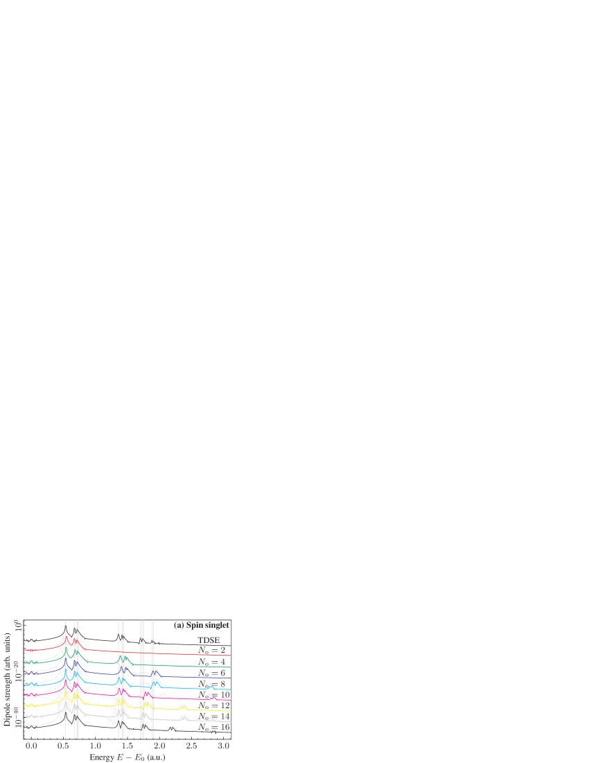
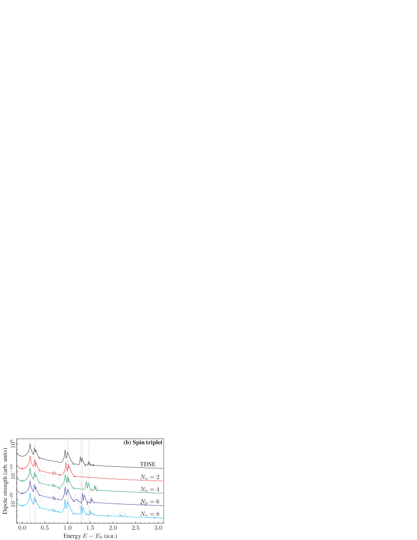
Figure 1: (Color online) Singlet (a) and triplet (b) linear response spectra for a different number of RNOs $N_{\mathrm{o}}$, compared to the exact TDSE result. For comparison, bare (i.e., with ground-state frozen Hamiltonian) TDRNOT results following the phase convention of section II.5.1 are shown with dashed lines. To guide the eyes, vertical lines indicate some of the distinct peaks in the exact TDSE spectrum.

As expected, the more series of doubly excited states are sought the more RNOs are needed. Interestingly, some peak positions of the spin singlet show an alternating convergence if one successively adds two RNOs more. For example, the peak around $E-E_{0}\approx 1.35$ is shifted to the wrong direction from $N_{\mathrm{o}}=4$ to $N_{\mathrm{o}}=6$ but substantially shifts towards its correct position for $N_{\mathrm{o}}=8$. Using $N_{\mathrm{o}}=10$, its peak position again slightly worsens compared to the previous value whereas for $N_{\mathrm{o}}=12$ the energy matches almost perfectly with the TDSE peak position.

The fully self-consistent time propagation using the PINO phase convention of section II.5.2 (solid) is clearly superior to the bare evolution with the phase convention of section II.5.1 (dashed gray): erroneous extra-peaks are absent, and the physical peaks are shifted to the correct TDSE positions. Both effects are particularly important for more RNOs, say $N_{\mathrm{o}}\geq 6$. Especially for the triplet, the full propagation with PINOs leads to much better results. The bare evolution generates erroneous extra peaks for any number of RNOs, corresponding to artificial states with nondegenerate ONs. Since degenerate ONs are a consequence of the exchange antisymmetry those peaks indicate the breaking of the exchange symmetry by the bare time evolution with the ground-state frozen Hamiltonian. This deficiency is removed by the full propagation using PINOs, as discussed in section III.2.

MCTDHF linear response spectra for the same model have been obtained in Hochstuhl et al. (2010). Our Fig. 1(a) can be directly compared with Fig. 3 there, where artificial extra peaks just above the first ionization threshold are seen. The reason for the erroneous peaks in the MCTDHF results is unknown to us. The superior performance of our TDRNOT approach using PINOs is presumably due to the built-in optimal choice of basis set functions at all times.

It is to be expected that our promising results translate to 3D two-electron systems. In fact, in Refs. giesbgritsbaer ; Meer it has been shown already that only a few of the highest occupied PINOs are sufficient to capture accurately the lowest excitations in the response of the 3D two-electron systems H₂ and HeH⁺.

IV.3 Rabi oscillations

Linear response spectra are not enough to study strong-field laser-matter interaction phenomena, which, by definition, are non-perturbative in nature and rely on electron dynamics far away from the ground state. A prime example for non-perturbative laser-matter coupling is Rabi oscillations. It has been shown that Rabi oscillations are not captured within “standard” TDDFT Ruggenthaler and Bauer (2009) but that XC functionals with memory, i.e., XC functionals beyond the adiabatic approximation, are required Helbig et al. (2011). It is important to understand that adiabatic TDDFT applied to Rabi oscillations may reproduce a reasonably looking position expectation value as a function of time Ruggenthaler and Bauer (2009) even though the time-dependent density is not properly described, especially at times of population inversion, e.g., after a $\pi$-pulse. Instead, the ONs $n_{k}(t)$ as a function of time are very sensitive entities, which we use for benchmarking our TDRNOT approach via a comparison with the exact TDSE result.

We consider a Rabi oscillation between the spin-singlet ground state and the first excited state, driven by a laser of resonant frequency $\omega=0.5337$. The vector potential amplitude $A=0.0125$ of the flat-top part is linearly ramped-up over four periods. Propagating eight different spatial NOs, we have $N_{\mathrm{o}}=16$. Due to the pairwise degeneracy follows $n_{1}(t)=n_{2}(t),\dots,n_{15}(t)=n_{16}(t)$ so that it is sufficient to discuss $n_{k\text{ odd}}(t)$.

The six most significant ONs $n_{1}(t),n_{3}(t),\dots,n_{11}(t)$ predicted by the TDRNOT propagation (solid) are compared with the exact TDSE result (dotted) in Fig. 2.

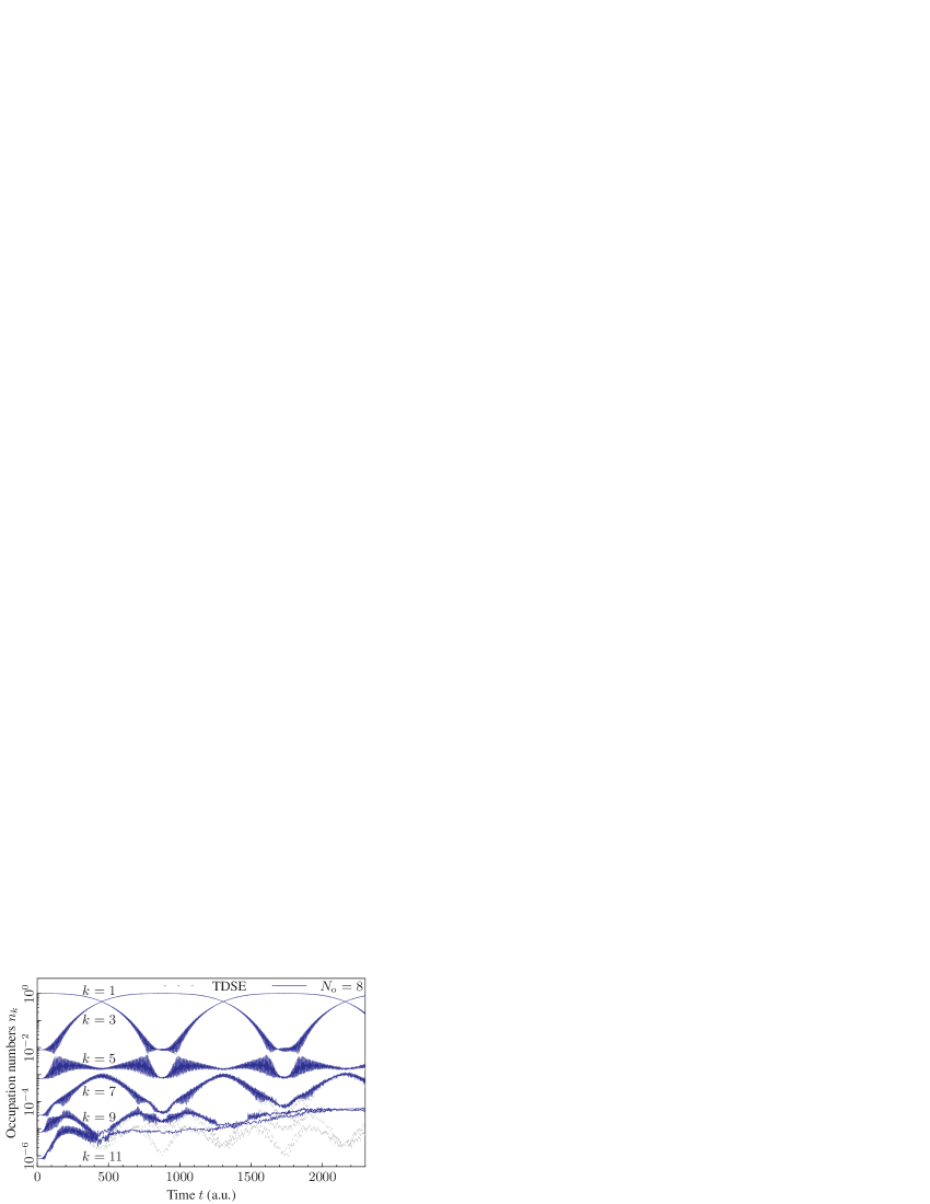
Figure 2: (Color online) ONs $n_{k}(t)$ vs time $t$ for the spin singlet in a laser field of frequency $\omega=0.5337$ resonantly tuned to the first excited state. The four most significant ONs $n_{1}(t),n_{3}(t),n_{5}(t),n_{7}(t)$ obtained by TDRNOT with $N_{\mathrm{o}}=16$ RNOs (solid) correctly reproduce more than two Rabi cycles of the exact TDSE propagation (dotted). Due to the truncation to a finite number of RNOs in TDRNOT, less significant orbitals are missing the proper coupling to lower orbitals, leading to erroneous behavior of small ONs over time. For longer propagation times also higher ONs are affected because the RNOs are coupled.

IV.3.1 Truncation problem

Thanks to the proper ground state description reported in section IV.1, all TDRNOT ONs start on top of the exact TDSE reference for $t=0$ in Fig. 2. However, already for small times $0<t\lesssim 200$ ONs $n_{13}(t)$ and $n_{15}(t)$ (not shown) begin to deviate from the correct value. Instead of the periodic oscillation with the Rabi period $2\text{\textpi}/\mathit{\Omega}_{\mathrm{R}}\approx 850$ and a modulation on the timescale of the laser period $2\text{\textpi}/\omega\approx 11.8$ they just approach their respective “upper neighbor” NO’s ON. The next ONs $n_{11}(t)$ and $n_{9}(t)$ become quantitatively distinguishable from their respective TDSE values around $t\gtrsim 400$ and $t\gtrsim 800$. After two Rabi cycles, i.e., $t\gtrsim 1700$ also their qualitative behavior is completely wrong, showing no oscillation on the Rabi timescale any longer. Around that time $t\approx 1700$ the next higher ON $n_{7}(t)$ is affected and shows some small quantitative differences compared to the exact solution, although it regains the proper behavior at later times.

The origin of these imperfections regarding the least significant orbitals in the propagation lies in the truncation to a finite number $N_{\mathrm{o}}=16$ of RNOs taken into account. The EOM in section III have been derived for an infinite number of coupled RNOs. It turns out that the orbital coupling via $\mathcal{B}_{nk}(t)$ is particularly strong for orbitals with nearby ONs so that the truncation of the orbitals $\{|\tilde{17}(t)\rangle,|\tilde{18}(t)\rangle,\dots\}$ is most severe for the least significant orbitals. Once their dynamics is spoiled, the truncation error subsequently propagates “upwards” due to the coupling to the respective next higher orbitals.

IV.3.2 Overall performance

The four most significant ONs $n_{1}(t)$, $n_{3}(t)$, $n_{5}(t)$, $n_{7}(t)$ in Fig. 2 are in a striking agreement with the exact TDSE result. Their dynamics during more than two Rabi cycles, i.e., a time period of 2300 atomic units in total, is well-described. Overall, the “well-behaved” RNOs represent more than $99.9\,\%$ of the 1-RDM so that the significant part of the Rabi dynamics is captured by TDRNOT.

The remarkable gain of TDRNOT compared to, e.g., TDDFT is that—despite the (numerically strongly favorable) locality in time—TDRNOT is capable of describing the highly resonant dynamics of Rabi oscillations. In fact, the exact two-electron TDRNOT EOM are strictly memory-free.

V Conclusion and outlook

In the current work, we have extended the previously introduced Brics and Bauer (2013) time-dependent renormalized natural orbital theory (TDRNOT). We have derived the equations of motion for renormalized natural orbitals, employing the phase convention in which the entire time-dependence is carried by the natural orbitals themselves. In the two-particle case, this allows to obtain the exact equations of motion, without making any assumptions about (or any approximations to) the expansion of the time-dependent two-body density matrix in natural orbitals. As an example, we have solved the equations of motion for a widely used helium model atom. In practical calculations, the number of natural orbitals taken into account should be as small as possible. As a truncation of the number of natural orbitals introduces numerical errors, we have benchmarked our results by the corresponding exact solutions of the time-dependent Schrödinger equation. Excellent agreement has been found for the spin-singlet and spin-triplet ground states (obtained via imaginary-time propagation), linear response spectra, and Rabi flopping dynamics (as an example for a strongly non-perturbative, resonant phenomenon).

We are mainly interested in laser-driven few-body correlated quantum dynamics. Besides Rabi flopping, we are currently applying the TDRNOT method successfully to other (strong-field) scenarios where “standard” time-dependent density functional theory with practicable exchange-correlation potentials is known to fail, e.g., nonsequential double ionization. Moreover, we are investigating the structure of the exact expansion coefficients $\tilde{\gamma}_{2,ijkl}$ for three-electron systems in order to derive useful expressions that can be used to propagate the respective natural orbitals using TDRNOT.

Appendix A Expansion of a two-fermion state in RNOs

Let the expansion of a two-fermion state $|\mathit{\Psi}(t)\rangle$ in orthonormal single-particle basis functions $|\psi_{i}(t)\rangle$ comprising spin and spatial degrees of freedom be

$$|\mathit{\Psi}(t)\rangle =\sum_{ij}\mathit{\Psi}_{ij}(t)|\psi_{i}(t),\psi_{j}(t)\rangle,$$

$$\mathit{\Psi}_{ij}(t) =\langle\psi_{i}(t),\psi_{j}(t)|\mathit{\Psi}(t)\rangle.$$

Defining a matrix $\bm{\mathit{\Psi}}=\left[\mathit{\Psi}_{ij}(t)\right]$ of expansion coefficients $\mathit{\Psi}_{ij}(t)$, the exchange antisymmetry can be expressed as $\bm{\mathit{\Psi}}^{\mathrm{T}}=-\bm{\mathit{\Psi}}$. With

$$\bm{\psi} =\begin{pmatrix}|\psi_{1}(t)\rangle\\ |\psi_{2}(t)\rangle\\ \vdots\end{pmatrix}, \bm{\psi}^{\ast} =\begin{pmatrix}\langle\psi_{1}(t)|\\ \langle\psi_{2}(t)|\\ \vdots\end{pmatrix},$$

$$\bm{\psi}^{\mathrm{T}} =\begin{pmatrix}|\psi_{1}(t)\rangle,|\psi_{2}(t)\rangle,\dots\end{pmatrix}, \bm{\psi}^{\dagger} =\begin{pmatrix}\langle\psi_{1}(t)|,\langle\psi_{2}(t)|,\dots\end{pmatrix}$$

such that

$$\bm{\psi}^{\ast}\bm{\psi}^{\dagger} =\begin{pmatrix}\langle\psi_{1}(t)|\\ \langle\psi_{2}(t)|\\ \vdots\end{pmatrix}\begin{pmatrix}\langle\psi_{1}(t)|,\langle\psi_{2}(t)|,\dots\end{pmatrix}$$

$$=\begin{pmatrix}\langle\psi_{1}(t),\psi_{1}(t)|&\langle\psi_{1}(t),\psi_{2}(t)|&\dots\\ \langle\psi_{2}(t),\psi_{1}(t)|&\langle\psi_{2}(t),\psi_{2}(t)|&\dots\\ \vdots&\vdots&\ddots\end{pmatrix}$$

the relation between a two-fermion state $|\mathit{\Psi}(t)\rangle$ and its coefficient matrix $\bm{\mathit{\Psi}}$ in the basis $\{|\psi_{i}(t)\rangle\}$ may be written as

$$\bm{\mathit{\Psi}} =\bm{\psi}^{\ast}\bm{\psi}^{\dagger}|\mathit{\Psi}(t)\rangle, |\mathit{\Psi}(t)\rangle =\bm{\psi}^{\mathrm{T}}\bm{\mathit{\Psi}}\bm{\psi}.$$ (48)

The skew-symmetric matrix $\bm{\mathit{\Psi}}=-\bm{\mathit{\Psi}}^{\mathrm{T}}$ can be factorized into unitary matrices $\bm{U},\bm{U}^{\dagger}$ and a block-diagonal matrix $\bm{\Sigma}$ as (Horn and Johnson, 2012, Corollary 2.6.6. (b))

$$\bm{\mathit{\Psi}} =\bm{U}\bm{\Sigma}\bm{U}^{\mathrm{T}}, \bm{\Sigma} =\operatorname{diag}(\bm{\Sigma}_{1},\bm{\Sigma}_{3},\bm{\Sigma}_{5},\dots),$$

$$\bm{\Sigma}_{i} =\begin{pmatrix}0&\xi_{i}(t)\\ -\xi_{i}(t)&0\end{pmatrix}, i \text{ odd}.$$

Inserting this factorization into (48), one obtains an expansion in the transformed basis $\bm{\phi}=\bm{U}^{\mathrm{T}}\bm{\psi}$,

$$|\mathit{\Psi}(t)\rangle =\bm{\psi}^{\mathrm{T}}\left(\bm{U}\bm{\Sigma}\bm{U}^{\mathrm{T}}\right)\bm{\psi}=\bm{\phi}^{\mathrm{T}}\bm{\Sigma}\bm{\phi}.$$

In other words, any two-fermion state $|\mathit{\Psi}(t)\rangle$ can be written in the form

$$|\mathit{\Psi}(t)\rangle =\sum_{i\text{ odd}}\xi_{i}(t)\Big{[}|\phi_{i}(t),\phi_{i^{\prime}}(t)\rangle-|\phi_{i^{\prime}}(t),\phi_{i}(t)\rangle\Big{]}$$ (49)

where the prime operator (14) was used. Inserting (49) into the 1-RDM (2) gives

$$\hat{\gamma}_{1}(t) =\sum_{k\text{ odd}}2|\xi_{k}(t)|^{2}\Big{[}|\phi_{k}(t)\rangle\langle\phi_{k}(t)|+|\phi_{k^{\prime}}(t)\rangle\langle\phi_{k^{\prime}}(t)|\Big{]},$$

which proves that $|k(t)\rangle=|\phi_{k}(t)\rangle$, i.e., the set $\{|\phi_{k}(t)\rangle\}$ is a set of NOs. The corresponding eigenvalues $2|\xi_{k}(t)|^{2}$ for odd $k$, i.e., the ONs, are (at least) pairwise degenerate,

$$n_{k}(t) =n_{k+1}(t)=2|\xi_{k}(t)|^{2}, k \text{ odd}.$$

Writing $\xi_{k}(t)=\tfrac{1}{\sqrt{2}}\mathrm{e}^{\mathrm{i}\varphi_{k}(t)}\sqrt{n_{k}(t)}$ for odd $k$, and switching to RNOs $\{|\tilde{k}(t)\rangle\}$, a two-fermion state reads

$$|\mathit{\Psi}(t)\rangle=\sum_{k\text{ odd}}\frac{\mathrm{e}^{\mathrm{i}\varphi_{k}(t)}}{\sqrt{2n_{k}(t)}}\Big{[}|\tilde{k}(t),\tilde{k}^{\prime}(t)\rangle-|\tilde{k}^{\prime}(t),\tilde{k}(t)\rangle\Big{]}.$$ (50)

Appendix B Factorization of RNOs in the triplet cases

Section II.3.2 contains a brief discussion of the very simple RNO factorization for the spin-triplet configuration $|\mathit{\Psi}\rangle_{\sigma}=\left|\uparrow\uparrow\right\rangle_{\sigma}$. The case $|\mathit{\Psi}\rangle_{\sigma}=\left|\downarrow\downarrow\right\rangle_{\sigma}$ is analogous. The factorization of the NOs for the spin triplet

$$|\mathit{\Psi}\rangle_{\sigma} =\frac{1}{\sqrt{2}}\left[\left|\uparrow\downarrow\right\rangle_{\sigma}+\left|\downarrow\uparrow\right\rangle_{\sigma}\right]$$ (51)

is more involved. Considering both positive and negative indices $k$ one may define RNOs

$$|\tilde{k}(t)\rangle =\begin{cases}|\tilde{k}(t)\rangle_{x}&\text{if $k>0$}\\ |-\tilde{k}(t)\rangle_{x}&\text{if $k<0$}\end{cases}\otimes\begin{cases}\left|\uparrow\right\rangle_{\sigma}&\text{if $k>0$, $k\text{ odd}$}\\ \left|\downarrow\right\rangle_{\sigma}&\text{if $k>0$, $k\text{ even}$}\\ \left|\downarrow\right\rangle_{\sigma}&\text{if $k<0$, $k\text{ odd}$}\\ \left|\uparrow\right\rangle_{\sigma}&\text{if $k<0$, $k\text{ even}$}\end{cases},$$

and a generalized prime operator acting on nonzero integer numbers $k$ according

$$k^{\prime} =\begin{cases}k+1&\text{if $k>0$, $k\text{ odd}$}\\ k-1&\text{if $k>0$, $k\text{ even}$}\\ k-1&\text{if $k<0$, $k\text{ odd}$}\\ k+1&\text{if $k<0$, $k\text{ even}$}\end{cases}.$$

Insertion into (13) (where now both positive and negative $k$ have to be considered in the sum) yields, again, the same structure (23) and the same $|\tilde{k}(t)\rangle_{x}$ as the other triplet configurations. If the Hamiltonian (32) does not act on spin degrees of freedom, as it is the case for the model He atom considered, the sole significance of the spin component of the state $|\mathit{\Psi}(t)\rangle$ is its effect on the exchange symmetry of the spatial part, which is the same for each of the three triplet configurations.

Appendix C Derivation of $\alpha_{kk}$ for PINOs

Writing (13) as

$$|\mathit{\Psi}(t)\rangle =\sum_{i\text{ odd}}\xi_{i}(t)\left[|i,i^{\prime}\rangle-|i^{\prime},i\rangle\right], \xi_{i}(t) =\mathrm{e}^{\mathrm{i}\varphi_{i,0}}\sqrt{\frac{n_{i}(t)}{2}},$$ (52)

with the phase factors $\mathrm{e}^{\mathrm{i}\varphi_{i}}$ given by (31), yields, upon insertion into the right-hand-side of the TDSE

$$\hat{H}(t)|\mathit{\Psi}(t)\rangle=\mathrm{i}\partial_{t}|\mathit{\Psi}(t)\rangle$$ (53)

$$\hat{H}(t)|\mathit{\Psi}(t)\rangle =\mathrm{i}\sum_{i\text{ odd}}\left[\dot{\xi}_{i}(t)\left(|i,i^{\prime}\rangle-|i^{\prime},i\rangle\right)\right.$$

$$\qquad\left.+\xi_{i}(t)\left(|\dot{i},i^{\prime}\rangle-|\dot{i^{\prime}},i\rangle+|i,\dot{i^{\prime}}\rangle-|i^{\prime},\dot{i}\rangle\right)\right].$$

Multiplying from the left by $\langle k,k^{\prime}|$ for an odd $k$ gives

$$\langle k,k^{\prime}|\hat{H}(t)|\mathit{\Psi}(t)\rangle =\mathrm{i}\dot{\xi}_{k}(t)+\xi_{k}(t)\left[\vphantom{\hat{h}(t)}\langle k|\partial_{t}|k\rangle+\langle k^{\prime}|\partial_{t}|k^{\prime}\rangle\right]=\mathrm{i}\frac{\dot{n}_{k}(t)}{2n_{k}(t)}\xi_{k}(t)+\mathrm{i}\xi_{k}(t)\left[\vphantom{\hat{h}(t)}\alpha_{kk}(t)+\alpha_{k^{\prime}k^{\prime}}(t)\right].$$ (54)

Insertion of (52) into the left-hand-side of the TDSE (53) gives

$$\langle k,k^{\prime}|\hat{H}(t)|\mathit{\Psi}(t)\rangle =\xi_{k}(t)\left[\langle k|\hat{h}(t)|k\rangle+\langle k^{\prime}|\hat{h}(t)|k^{\prime}\rangle\right]+\sum_{i\text{ odd}}\xi_{i}(t)\left[\vphantom{\hat{h}(t)}\langle k,k^{\prime}|{v_{\mathrm{ee}}}|i,i^{\prime}\rangle-\langle k,k^{\prime}|{v_{\mathrm{ee}}}|i^{\prime},i\rangle\right].$$ (55)

Combination of (54) and (55) yields

$$\alpha_{kk}(t)+\alpha_{k^{\prime}k^{\prime}}(t) =\langle k|\hat{h}(t)|k\rangle+\langle k^{\prime}|\hat{h}(t)|k^{\prime}\rangle+\sum_{i\text{ odd}}\frac{\xi_{i}(t)}{\xi_{k}(t)}\left[\vphantom{\hat{h}(t)}\langle k,k^{\prime}|{v_{\mathrm{ee}}}|i,i^{\prime}\rangle-\langle k,k^{\prime}|{v_{\mathrm{ee}}}|i^{\prime},i\rangle\right]-\mathrm{i}\frac{\dot{n}_{k}(t)}{2n_{k}(t)}.$$ (56)

Recasting the sum in (56) in the form

$$\frac{2}{n_{k}(t)}\sum_{i\text{ odd}}\mathrm{e}^{\mathrm{i}\left(\varphi_{i,0}-\varphi_{k,0}\right)}\sqrt{\frac{n_{i}(t)}{2}}\sqrt{\frac{n_{k}(t)}{2}}\left[\vphantom{\hat{h}(t)}\langle k,k^{\prime}|{v_{\mathrm{ee}}}|i,i^{\prime}\rangle-\langle k,k^{\prime}|{v_{\mathrm{ee}}}|i^{\prime},i\rangle\right] =\frac{2}{n_{k}(t)}\sum_{ijl}\tilde{\gamma}_{2,ijkl}(t)\langle\tilde{k}\tilde{l}|{v_{\mathrm{ee}}}|\tilde{i}\tilde{j}\rangle$$ (57)

and making use of the analytically known expression for $\dot{n}_{k}(t)$ Brics and Bauer (2013),

$$\dot{n}_{k}(t) =4\operatorname{Im}\sum_{ijl}\tilde{\gamma}_{2,ijkl}(t)\langle\tilde{k}\tilde{l}|{v_{\mathrm{ee}}}|\tilde{i}\tilde{j}\rangle,$$ (58)

gives

$$\alpha_{kk}(t)+\alpha_{k^{\prime}k^{\prime}}(t) =\langle k|\hat{h}(t)|k\rangle+\langle k^{\prime}|\hat{h}(t)|k^{\prime}\rangle+\frac{2}{n_{k}(t)}\operatorname{Re}\sum_{ijl}\tilde{\gamma}_{2,ijkl}(t)\langle\tilde{k}\tilde{l}|{v_{\mathrm{ee}}}|\tilde{i}\tilde{j}\rangle.$$ (59)

Equation (59) reflects the freedom to distribute the global phase of $|i,i^{\prime}\rangle-|i^{\prime},i\rangle$ in (52) among orbital $i$ and orbital $i^{\prime}$. Choosing

$$\alpha_{kk}(t) =\alpha_{k^{\prime}k^{\prime}}(t)-\langle k^{\prime}|\hat{h}(t)|k^{\prime}\rangle+\langle k|\hat{h}(t)|k\rangle$$ (60)

it is found that for both odd and even $k$ the final result reads

$$\alpha_{kk}(t)=\frac{1}{n_{k}(t)}\left[\langle\tilde{k}|\hat{h}(t)|\tilde{k}\rangle+\operatorname{Re}\sum_{ijl}\tilde{\gamma}_{2,ijkl}(t)\langle\tilde{k}\tilde{l}|{v_{\mathrm{ee}}}|\tilde{i}\tilde{j}\rangle\right].$$ (61)

Appendix D Variational determination of the spin-triplet ground state

As in Brics and Bauer (2013), we define an energy functional $\tilde{E}$ taking into account the constraints $\sum_{i}n_{i}=N=2$, $\langle i|j\rangle=\operatorname{\delta}_{ij}$, $n_{i}\geq 0$, $n_{i}\leq 1$ via the Lagrange parameters $\epsilon$ and $\lambda_{ij}$ as well as the Karush-Kuhn-Tucker parameters giesbthesis ; Nocedal and Wright (2006) $\epsilon_{i}^{0}$ and $\epsilon_{i}^{1}$, respectively. Additionally, the degeneracy $n_{i}=n_{i^{\prime}}$ is enforced via the Lagrange parameter $\epsilon_{i}^{\mathrm{d}}$ for odd $i$. The functional $\tilde{E}$ reads

$$\tilde{E} =\sum_{i}\langle\tilde{i}|\hat{h}_{0}|\tilde{i}\rangle+\sum_{ijkl}\frac{\mathit{\Gamma}_{2,ijkl}}{\sqrt{\langle\tilde{i}|\tilde{i}\rangle\langle\tilde{k}|\tilde{k}\rangle}}\langle\tilde{k}\tilde{l}|{v_{\mathrm{ee}}}|\tilde{i}\tilde{j}\rangle$$

$$\quad-\epsilon\left[\vphantom{\sum_{i}}\sum_{i}\langle\tilde{i}|\tilde{i}\rangle-2\right]-\sum_{i}\sum_{j\neq i}\lambda_{ij}\langle\tilde{i}|\tilde{j}\rangle-\sum_{i}\left[\vphantom{\sum_{i}}\epsilon_{i}^{0}\langle\tilde{i}|\tilde{i}\rangle+\epsilon_{i}^{1}\left(1-\langle\tilde{i}|\tilde{i}\rangle\right)\right]-\sum_{i\text{ odd}}\epsilon_{i}^{\mathrm{d}}\left[\vphantom{\sum_{i}}\langle\tilde{i}|\tilde{i}\rangle-\langle\tilde{i^{\prime}}|\tilde{i^{\prime}}\rangle\right],$$ (62)

where the slackness conditions giesbthesis are $0=\epsilon_{i}^{0}n_{i}=\epsilon_{i}^{1}(1-n_{i})$, and

$$\mathit{\Gamma}_{2,ijkl}=(-1)^{i-k}\frac{\mathrm{e}^{\mathrm{i}\left(\varphi_{i,0}-\varphi_{k,0}\right)}}{2}\operatorname{\delta}_{ij^{\prime}}\operatorname{\delta}_{kl^{\prime}},$$

which is a constant regarding the variation of RNOs. Variation of the energy functional (62) with respect to $\langle\tilde{m}|$ and $|\tilde{m}\rangle$ yields

$$\epsilon_{m}|\tilde{m}\rangle =\left\{\hat{h}_{0}+2\sum_{jl}\frac{\mathit{\Gamma}_{2,mjml}}{\langle\tilde{m}|\tilde{m}\rangle}\langle\tilde{l}|{v_{\mathrm{ee}}}|\tilde{j}\rangle(x)-\frac{1}{\langle\tilde{m}|\tilde{m}\rangle}\operatorname{Re}\left[\sum_{ijl}\frac{\mathit{\Gamma}_{2,ijml}}{\sqrt{\langle\tilde{i}|\tilde{i}\rangle\langle\tilde{m}|\tilde{m}\rangle}}\langle\tilde{m}\tilde{l}|{v_{\mathrm{ee}}}|\tilde{i}\tilde{j}\rangle\right]\right\}|\tilde{m}\rangle$$

$$\qquad\qquad+\sum_{i\neq m}\left\{2\sum_{jl}\frac{\mathit{\Gamma}_{2,ijml}}{\sqrt{\langle\tilde{i}|\tilde{i}\rangle\langle\tilde{m}|\tilde{m}\rangle}}\langle\tilde{l}|{v_{\mathrm{ee}}}|\tilde{j}\rangle(x)-\lambda_{mi}\right\}|\tilde{i}\rangle$$ (63)

and its Hermitian conjugate, respectively. The orbital energies $\epsilon_{m}$ are defined as

$$\epsilon_{m} =\epsilon+\epsilon_{m}^{0}-\epsilon_{m}^{1}+\epsilon^{\mathrm{d}}_{m}\operatorname{\delta}_{m\text{ odd}}-\epsilon^{\mathrm{d}}_{m-1}\operatorname{\delta}_{m\text{ even}}.$$

The phases $\varphi_{i,0}$ in (31) are defined such that the ground state NOs of the model system may be chosen real. Assuming real ground state NOs, (63) and its Hermitian conjugate yield

$$\epsilon_{k} =\frac{1}{n_{k}}\left[\langle\tilde{k}|\hat{h}_{0}|\tilde{k}\rangle+\sum_{ijl}\tilde{\gamma}_{2,ijkl}\langle\tilde{k}\tilde{l}|{v_{\mathrm{ee}}}|\tilde{i}\tilde{j}\rangle\right].$$

For correlated systems, i.e., in general non-integer ONs, we have $0=\epsilon_{i}^{0}=\epsilon_{i}^{1}$ so that $\epsilon_{k}=\epsilon+\epsilon^{\mathrm{d}}_{m}\operatorname{\delta}_{m\text{ odd}}-\epsilon^{\mathrm{d}}_{m-1}\operatorname{\delta}_{m\text{ even}}$. Hence, each sum of two associated orbital energies in the ground state fulfills

$$\epsilon_{k}+\epsilon_{k^{\prime}} =2\epsilon.$$

Moreover, the set of ground state RNOs is a stationary point of the imaginary-time propagation, as already pointed out for the singlet in Brics and Bauer (2013).

Appendix E Newton scheme for finding ground state ONs

In this appendix, a scheme for finding the correct ground state ONs is presented when the phase convention of section II.5.1 is chosen. Section III.1 contains a brief discussion why this “tuning” of ONs is necessary. The variational calculus in appendix D shows that the converged RNOs associated with the correct ground state ONs fulfill

$$\epsilon_{k}+\epsilon_{k^{\prime}} =E=E_{0}.$$ (64)

For $N_{\mathrm{o}}$ RNOs, due to the pairwise degeneracy of ONs and the constraint $\sum_{k}n_{k}=2$, there are $(N_{\mathrm{o}}/2-1)$ free parameters. With

$$n_{1}=n_{2} =1-\sum_{\text{odd }i\neq 1}n_{i}$$ (65)

and

$$\bm{n} =\left(n_{3},n_{5},\dots,n_{N_{\mathrm{o}}-1}\right)^{\mathrm{T}},$$

$$\bm{F}(\bm{n}) =\left(F_{3}(\bm{n}),F_{5}(\bm{n}),\dots,F_{N_{\mathrm{o}}-1}(\bm{n})\right)^{\mathrm{T}},$$

$$F_{m}(\bm{n}) =\epsilon_{m}+\epsilon_{m+1}-\epsilon_{1}-\epsilon_{2}$$

the root of $\bm{F}$ fulfills (64) for all $k$. We thus search the root of $\bm{F}$ using the Newton-Raphson scheme. One iteration step from configuration $\bm{n}^{(i)}$ to configuration $\bm{n}^{(i+1)}$ is performed according to

$$\bm{J}\left(\bm{n}^{(i+1)}-\bm{n}^{(i)}\right) =-\bm{F}(\bm{n}^{(i)})$$

where $\bm{J}=\left[J_{mn}\right]=\left[\partial_{n_{n}}F_{m}\right]$ (for odd $m\neq 1$ and odd $n\neq 1$) is the Jacobian matrix. The derivatives $\partial_{n_{n}}F_{m}$ are calculated using

$$\partial_{n_{n}}|\tilde{m}\rangle =|m\rangle\partial_{n_{n}}\sqrt{n_{m}}.$$ (66)

In practice, also the converged NOs $|m_{0}(\bm{n})\rangle$ for a given ON configuration $\bm{n}$ change if the ON $n_{n}$ (and thus also $n_{1}$, $n_{2}$, and $n_{n^{\prime}}$) is modified. However, the approximation (66) yields smooth convergence. Because of (65) $\partial_{n_{n}}n_{1}=-1$ for odd $n\neq 1$. Hence for odd $n\neq 1$

$$\partial_{n_{n}}\gamma_{2,ijkl} =\left[\operatorname{\delta}_{ni}+\operatorname{\delta}_{nj}+\operatorname{\delta}_{nk}+\operatorname{\delta}_{nl}\right]\frac{\gamma_{2,ijkl}}{2n_{n}}-\left[\operatorname{\delta}_{1i}+\operatorname{\delta}_{1j}+\operatorname{\delta}_{1k}+\operatorname{\delta}_{1l}\right]\frac{\gamma_{2,ijkl}}{2n_{1}}.$$

Assuming real NOs for the ground state one finds for odd $m\neq 1$

$$F_{m} =\langle m|\hat{h}_{0}|m\rangle+\langle m^{\prime}|\hat{h}_{0}|m^{\prime}\rangle+2\sum_{ij}\frac{\gamma_{2,ijmm^{\prime}}}{n_{m}}\langle mm^{\prime}|{v_{\mathrm{ee}}}|ij\rangle-\langle 1|\hat{h}_{0}|1\rangle-\langle 2|\hat{h}_{0}|2\rangle-2\sum_{ij}\frac{\gamma_{2,ij12}}{n_{1}}\langle 12|{v_{\mathrm{ee}}}|ij\rangle.$$

The phases $\varphi_{i}$ in $\gamma_{2,ijkl}$ can be set to the frozen phases $\varphi_{i,0}$ of the PINO phase convention (31) because the time-independent ground state is sought. For odd $n\not\in\{1,m\}$ follows

$$\partial_{n_{n}}F_{m} =\frac{1}{2(n_{n}n_{m})^{3/2}}\langle\tilde{m}\tilde{m}^{\prime}|{v_{\mathrm{ee}}}\left[|\tilde{n}\tilde{n}^{\prime}\rangle-|\tilde{n}^{\prime}\tilde{n}\rangle\right]-\frac{\mathrm{e}^{\mathrm{i}\varphi_{m,0}}}{2(n_{1}n_{m})^{3/2}}\langle\tilde{m}\tilde{m}^{\prime}|{v_{\mathrm{ee}}}\left[|\tilde{1}\tilde{2}\rangle-|\tilde{2}\tilde{1}\rangle\right]$$

$$\qquad-\frac{\mathrm{e}^{\mathrm{i}\varphi_{n,0}}}{2(n_{n}n_{1})^{3/2}}\langle\tilde{1}\tilde{2}|{v_{\mathrm{ee}}}\left[|\tilde{n}\tilde{n}^{\prime}\rangle-|\tilde{n}^{\prime}\tilde{n}\rangle\right]-\sum_{\text{odd }i\neq 1}\frac{\mathrm{e}^{\mathrm{i}\varphi_{i,0}}}{2\sqrt{n_{1}^{5}n_{i}}}\langle\tilde{1}\tilde{2}|{v_{\mathrm{ee}}}\left[|\tilde{i}\tilde{i}^{\prime}\rangle-|\tilde{i}^{\prime}\tilde{i}\rangle\right],$$

for the diagonal element

$$\partial_{n_{m}}F_{m} =-\sum_{\text{odd }i\neq m}\frac{\mathrm{e}^{\mathrm{i}\left[\varphi_{m,0}+\varphi_{i,0}\right]}}{2\sqrt{n_{m}^{5}n_{i}}}\langle\tilde{m}\tilde{m}^{\prime}|{v_{\mathrm{ee}}}\left[|\tilde{i}\tilde{i}^{\prime}\rangle-|\tilde{i}^{\prime}\tilde{i}\rangle\right]-\sum_{\text{odd }i\neq 1}\frac{\mathrm{e}^{\mathrm{i}\varphi_{i,0}}}{2\sqrt{n_{1}^{5}n_{i}}}\langle\tilde{1}\tilde{2}|{v_{\mathrm{ee}}}\left[|\tilde{i}\tilde{i}^{\prime}\rangle-|\tilde{i}^{\prime}\tilde{i}\rangle\right]$$

$$\qquad-\frac{\mathrm{e}^{\mathrm{i}\varphi_{m,0}}}{(n_{1}n_{m})^{3/2}}\langle\tilde{m}\tilde{m}^{\prime}|{v_{\mathrm{ee}}}\left[|\tilde{1}\tilde{2}\rangle-|\tilde{2}\tilde{1}\rangle\right].$$

References

• (1) A. Scrinzi, in Attosecond and XUV Physics edited by Th. Schultz, M. Vrakking (Wiley-VCH, Weinheim, 2014), p. 257–292.
• (2) C.A. Coulson, Rev. Mod. Phys. 32, 170 (1960).
• Runge and Gross (1984) E. Runge and E. K. U. Gross, Phys. Rev. Lett. 52, 997 (1984).
• (4) C.A. Ullrich, Time-Dependent Density Functional Theory, Concepts and Applications, (Oxford University Press, Oxford, 2012).
• Helbig et al. (2011) N. Helbig, J. Fuks, I. Tokatly, H. Appel, E. Gross,  and A. Rubio, Chemical Physics 391, 1 (2011).
• (6) M. Petersilka, E.K.U. Gross, Laser Phys. 9, 105 (1999).
• (7) F. Wilken, D. Bauer, Phys. Rev. Lett. 97, 203001 (2006).
• (8) F. Wilken, D. Bauer, Phys. Rev. A76, 023409 (2007).
• (9) A.J. Coleman, V.I. Yukalov, Reduced Density Matrices, Coulson’s Challenge, Lecture Notes in Chemistry 72, (Springer, Berlin Heidelberg, 2000).
• (10) J. Cioslowski (Ed.), Many-electron densities and reduced density matrices, Mathematical and Computational Chemistry Series, (Kluwer/Plenum, New York, 2000).
• (11) N.I. Gidopoulos, S. Wilson (Eds.), Electron Density, Density Matrix and Density Functional Theory in Atoms, Molecules and the Solid State, Progress in Theoretical Chemistry and Physics, (Kluwer, Dordrecht, 2003).
• (12) D.A. Mazziotti (Ed.), Reduced-Density-Matrix Mechanics, Advances in Chemical Physics Vol. 134, (Wiley, Hoboken, 2007).
• (13) D.A. Mazziotti, Chem. Rev. 112, 244 (2012).
• (14) K. Pernal, O. Gritsenko, E.J. Baerends, Phys. Rev. A75, 012506 (2007)
• (15) H. Appel, Time-Dependent Quantum Many-Body Systems: Linear Response, Electronic Transport, and Reduced Density Matrices, (Doctoral Thesis, Free University Berlin, 2007); http://www.diss.fu-berlin.de/diss/receive/FUDISS_thesis_000000003068
• (16) K.J.H. Giesbertz, E.J. Baerends, O.V. Gritsenko, Phys. Rev. Lett. 101, 033004 (2008).
• (17) K.J.H. Giesbertz, Time-Dependent One-Body Reduced Density Matrix Functional Theory, Adiabatic Approximations and Beyond, (PhD Thesis, Free University Amsterdam, 2010); http://dare.ubvu.vu.nl/handle/1871/16289
• (18) R. Requist, O. Pankratov, Phys. Rev. A81, 042519 (2010).
• (19) H. Appel, E.K.U. Gross, Europhys. Lett. 92, 23001 (2010).
• (20) P.-O. Löwdin, Phys. Rev. 97, 1474 (1955).
• (21) P.-O. Löwdin, H. Shull, Phys. Rev. 101, 1730 (1956).
• (22) K.J.H. Giesbertz, Chem. Phys. Lett. 591, 220 (2014)
• (23) R. Grobe and J.H. Eberly, Phys. Rev. Lett. 68, 2905 (1992); S.L. Haan, R. Grobe, and J.H. Eberly, Phys. Rev. A50, 378 (1994).
• (24) D. Bauer, Phys. Rev. A56, 3028 (1997); D.G. Lappas and R. van Leeuwen, J. Phys. B: At. Mol. Opt. Phys. 31, L249 (1998); D. Bauer, F. Ceccherini, Phys. Rev. A60, 2301 (1999); M. Lein, E.K.U. Gross, and V. Engel, Phys. Rev. Lett. 85, 4707 (2000); M. Thiele, E.K.U. Gross, and S. Kümmel, Phys. Rev. Lett. 100, 153004 (2008).
• Brics and Bauer (2013) M. Brics and D. Bauer, Phys. Rev. A 88, 052514 (2013).
• (26) A.J. Krueger and N.T. Maitra, Phys. Chem. Chem. Phys. 11, 4655 (2009).
• (27) K.J.H. Giesbertz, O.V. Gritsenko, and E.J. Baerends, J. Chem. Phys. 136, 094104 (2012).
• (28) R. van Meer, O.V. Gritsenko, K.J.H. Giesbertz, and E.J. Baerends, J. Chem. Phys. 138, 094114 (2013).
• Hochstuhl et al. (2010) D. Hochstuhl, S. Bauch,  and M. Bonitz, Journal of Physics: Conference Series 220, 012019 (2010).
• Ruggenthaler and Bauer (2009) M. Ruggenthaler and D. Bauer, Phys. Rev. Lett. 102, 233001 (2009).
• Horn and Johnson (2012) R. Horn and C. Johnson, Matrix Analysis, 2nd ed. (Cambridge University Press, New York, 2012).
• Nocedal and Wright (2006) J. Nocedal and S. Wright, Numerical Optimization, 2nd ed., Springer Series in Operations Research and Financial Engineering (Springer, New York, 2006).