Geometric Abstraction from Noisy Image-Based 3D Reconstructions

Abstract

Creating geometric abstracted models from image-based scene reconstructions is difficult due to noise and irregularities in the reconstructed model. In this paper, we present a geometric modeling method for noisy reconstructions dominated by planar horizontal and orthogonal vertical structures. We partition the scene into horizontal slices and create an inside/outside labeling represented by a floor plan for each slice by solving an energy minimization problem. Consecutively, we create an irregular discretization of the volume according to the individual floor plans and again label each cell as inside/outside by minimizing an energy function. By adjusting the smoothness parameter, we introduce different levels of detail. In our experiments, we show results with varying regularization levels using synthetically generated and real-world data.

1 Introduction

Thanks to recent advances in image-based 3D reconstruction techniques like Structure-from-Motion [9] (SfM) and patch-based multi view stereo [5] (PMVS) and the availability of depths sensors like Time-of-Flight cameras or with structured light technology, we can easily create large-scale, high-resolution 3D reconstructions containing millions of points.

However, transmitting, visualizing, processing and analyzing the acquired data is far from practical use within applications. For example, to transmit a point cloud of millions of points over the Internet is not possible in reasonable time and therefore abstracted models are desired. Further, to extract semantic information out of a 3D reconstruction, it has to be separated into semantic meaningful parts first. For example, by separating a building model into floors, a floor plan can be extracted for each level and can be processed individually.

There exist several approaches for representing a 3D model in a simplified way. In Wu et al. [10], a parametric method for reconstructing architectural scenes from sparse point clouds is proposed. Profile curves are swept over a network of transport curves in order to generate swept surfaces.

Xiao and Furukawa [11] introduce a method to automatically construct and visualize 3D models for large indoor scenes using 3D laser scanner data as input. Their approach partitions the 3D model into horizontal slices, which are bounded by dominant horizontal structures. For each slice, walls are detected by projecting all laser points to the 2D ground plane and then using a Hough transform to detect lines. Each floor plan is approximated by a 2D Constructive Solid Geometry (CSG) representation. To obtain a full 3D model, the 2D CSG representation is lifted into 3D and again optimized to obtain consistent 3D models. If the condition that the scene purely consists of vertical structures is violated or the 3D data is perturbed by significant amount of noise, the wall detection using Hough lines fails and the overall result degrades. Therefore this approach is not suited for SfM results that contain significant amount of noise and outliers.

A similar approach for multi-level indoor scenes (i.e., whole buildings) which is not limited to orthogonal or parallel structures is proposed by Oesau et al. [8]. First, permanent structures (wall, floor, ceiling) are detected using horizontal slicing and wall directions are computed using Hough transform. For every slice, a triangular decomposition is created and extruded to 3D to form irregularly shaped volumetric cells. Finally, the volumetric cells are labeled as empty or occupied space by optimizing an energy function that is modeled by a conditional random field (CRF). In comparison to [11], this approach improves the handling of rounded vertical structures. Though, it also assumes laser data with little noise as input data.

In this paper, we focus on extracting meaningful geometric structures of man-made environments which are often dominated by planar surfaces. In contrast to the work of [11] and [8] that rely on clean input data obtained by a laser scanner, we focus on surface meshes as they are created by standard image-based reconstruction pipelines like PMVS combined with meshing techniques like Poisson triangulation [6] . Compared to laser scan data, the mesh has a much higher level of noise and often contains artifacts which complicates the extraction of a simplified geometry.

Following the idea of [11], we first identify horizontal slices that are limited by dominant horizontal planar structures. For each slice, we generate a 2D floor plan by solving an inside/outside labeling problem in a global optimal manner formulating an energy minimization problem. In order to integrate all floor plans into a consistent 3D model, we create an irregular discretization of the volume according to the individual floor plans. The obtained volume elements are again labeled as inside/outside by minimizing an energy function. For an individual building, the whole procedure results in a set of floor plans and an adjustably regularized geometric abstraction of the input 3D point cloud. In our experimental evaluation, we show that our approach massively simplifies the input mesh while the results are geometrically consistent with the input data. We demonstrate that our approach is computationally efficient and delivers accurate results where existing methods may fail.

2 Our Approach

Given a meshed point cloud and the corresponding camera poses $C$ as input, we want to extract relevant geometric structures of the scene. As precondition, we assume that it is dominated by planar horizontal and orthogonal vertical surfaces. We apply preprocessing steps to transform the model to a new coordinate system aligned with a reference plane and perform a predefined, constant upsampling of the meshed point cloud. At dominant horizontal structures, we partition the model into horizontal slices. A slice represents a part of the model which includes mainly vertical structures and is bounded by horizontal structures. For each slice, we create a 2D floor plan using the visibility information. The individual floor plans are used to create an irregular discretization of the volume into cells. Finally, we obtain a regularized 3D model by labeling each cell as inside/outside using a CRF. Fig. 1 illustrates the different modules of our processing workflow.

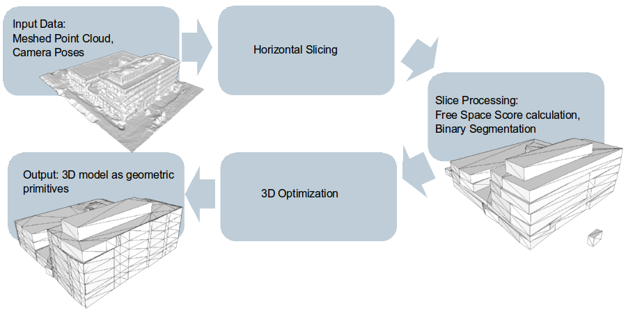
Figure 1: Overview of our processing workflow.

2.1 Slicing and Contour Extraction

In this section, we describe the processing of the point cloud in the slice domain. Initially, the model gets partitioned into horizontal slices. A slice includes similar vertical structures, e.g. vertical walls, and is bounded by horizontal structures. For each slice we calculate a 2D binary segmentation resulting in a floor plan. The segmentation is performed by using the visibility information that is associated with the input mesh. Finally, we approximate the border of the segmentation with line segments.

Slice Extraction. In our workflow, slices are defined as parts of the model enclosed by dominant horizontal structures. We find these structures by projecting points with normals similar to the ground plane normal, i.e. similar to the z-axis, onto the z-axis. On this one-dimensional data, we perform mode estimation using mean shift [2]. We use the centers of the modes as boundaries of the slices.

The mean shift bandwidth is calculated as a fraction of the model height. This leads to independence of the model size and just the denominator $d$ has to be defined: $bandwidth=\frac{height}{d}.$ By adjusting the bandwidth parameter of mean shift, it is possible to generate slice boundaries at all minor horizontal structures or just at the most important dominant structures. Thus, the parameter $d$ defines the potential level of detail in the vertical direction of our modeling approach.

Binary Segmentation. In order to identify the dominant vertical structures of each slice, we perform a binary inside/outside segmentation in the discretized 2D slice plane. The discontinuity between differently labeled regions is then the resulting 2D floor plan. Visibility information is used to define a probability for every pixel for being inside or outside of the object. We call this probability free space score. Finally, we define an energy function to obtain an optimal labeling.

To calculate the free space score for each pixel in 2D, we first create a voxel grid spanned over the whole scene and assign each voxel a score for being free and occupied space. This score is defined by the number of cameras a certain voxel is visible in. Therefore, we cast rays from each voxel $v_{xyz}$ to all camera centers $C$. If a ray from $v_{xyz}$ to a camera $c\in C$ does not intersect the input mesh, $v_{xyz}$ is visible in $c$. The score that $v_{xyz}$ is in free space is defined as

$$p(v_{xyz}=outside|visibility)=\frac{\{\#\ cameras\ v_{xyz}\ is\ visible\ in\}}{\{max\ \#\ visible\ cameras\}},$$ (1)

where $\{max\ \#\ visible\ cameras\}$ is the maximum number of visible cameras for a voxel $v_{xyz}$.
For all the voxels $v_{xyz}\in V$ which have not been visible in any camera view, we define the score that $v_{xyz}$ is in occupied space by calculating the distance of $v_{xyz}$ to the next voxel $v_{xyz}^{\prime}$ that is in free space, i.e.  $p(v_{xyz}^{\prime}=free|visibility)>0$:

$$p(v_{xyz}=inside|visibility)=\frac{\min(dist(v_{xyz},v_{xyz}^{\prime}),maxDist)}{maxDist},$$ (2)

where $dist(\cdot)$ calculates the Euclidean distance between the voxel centers and $maxDist$, which is a predefined maximum distance, truncates this distance. Hence, this formula is closely related to the truncated signed distance function [12] which is used for example in surface extraction algorithms.

Given the free space scores for each voxel, we can easily define the scores for each pixel $b_{xy}$ in the 2D slice plane by averaging the scores of the voxels:

$$p(b_{xy}=free|visibility)=\sum_{z}\frac{p(v_{xyz}=free|visibility)}{n},$$ (3)

where $n$ is the voxel dimension in z-direction of the slice. The score that a pixel is occupied is defined in the same way.

Finally, we obtain an optimal inside/outside labeling of the 2D slice plane by solving an energy minimization problem where we directly use the defined free space scores as data term. The pairwise terms are defined by the Potts model.

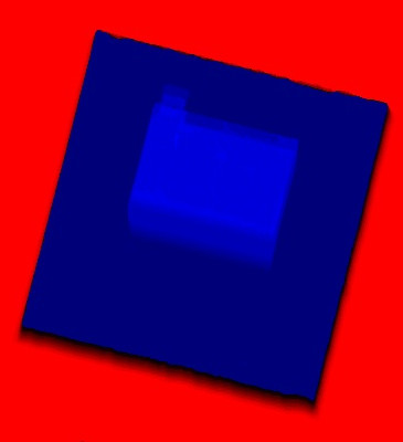
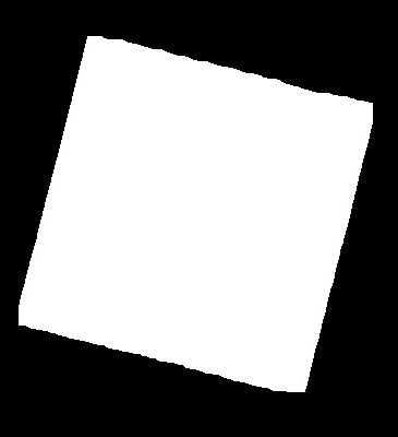
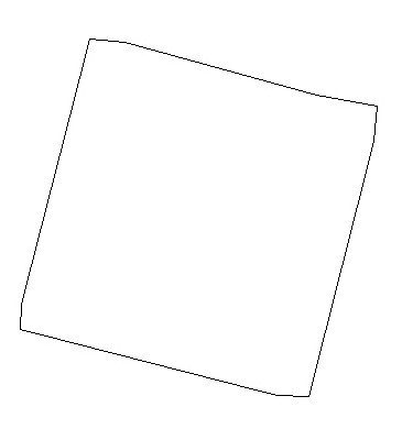
Figure 2: Slice processing. Left, the free space scores projected to 2D are illustrated. All voxels within a slice are projected onto a 2D matrix and a free space score per pixel gets calculated (blue means inside, red outside). Using graph cut energy minimization, a binary labeling for inside and outside is calculated (middle). On the binary labeling, outline simplification is applied which delivers a polygonal line (right).

Outline Simplification. For the creation of the geometric 3D model, we just need the outline of the inside-labeled pixels. Though, as the outline is a polygonal line including every pixel as point and we favor simple representations, a simplification of the polygonal outline is applied before continuing with further processing steps. There exist several approaches for this task. We use the Ramer-Douglas-Peucker algorithm [4] in our implementation. The algorithm produces a polygonal line as in Fig. 2, which can be easily extruded to 3D.

2.2 Slice Combination

By extruding the object outlines from each slice to 3D (as in Fig. 3), we can already create a regularized 3D model. However, as you can see in the labeling masks of the two slices, there usually exist small differences in the 2D discretization which result in non-smooth 3D models. Further, small irregularities that just occur in one slice are not necessarily wanted to be in the geometric model. Therefore, we apply a regularization step by partitioning the whole possible occupied space into irregularly shaped 3D volumetric cells and create again an optimal inside/outside labeling using energy minimization.

Volumetric Cells. To regularize the geometric model, we partition the model into irregularly shaped volumetric cells. The concept is illustrated in Fig. 3. We define volumetric cells as right prisms with triangles as base faces.

For the partitioning, we first project all object outlines of each slice’s binary segmentation to the ground plane. Next, we apply a Constrained Delaunay Triangulation (CDT) to this line set. The CDT guarantees that the projected outlines remain lines in the final triangulation. Finally, we extrude the triangles between all slice boundaries to get an irregular space partitioning of the whole scene.

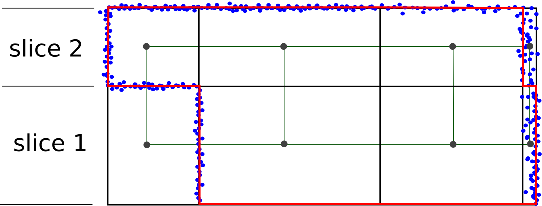
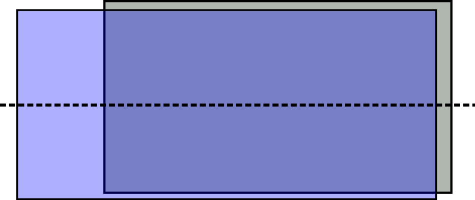
Figure 3: Left: Volumetric Cells. Vertical cut of a volumetric cell representation of a simple model consisting out of two slices. The black lines are the volumetric cells spanned over the whole scene and the red lines are the outlines of the extruded slices approximating the point cloud (blue dots). A graph is spanned over the whole scene setting cells with a shared face as neighbors (green lines). Right: Top-view of binary labeling of both slices. As you can see, a noisy point cloud leads to slightly varying object outlines in each slice. The dashed line represents the vertical cut seen in the left image.

3D Regularization. To get rid of unwanted irregularities between the different slices, we perform a regularization in 3D. Given the volumetric cell representation, we want to find an optimal inside/outside labeling for the cells. Similar to the slice binarization, we use the visibility information to setup an energy optimization problem that is formulated as an CRF:

$$E(L)=\sum_{p\in\mathcal{I}}E_{data}(L(p))+\lambda\sum_{p,q\in\mathcal{N}}E_{smooth}(L(p),L(q)),$$ (4)

where $\mathcal{I}$ denotes the set of all volumetric cells, $\mathcal{N}$ is the neighborhood of every cell and $L$ is the (binary) labeling. The neighborhood relation is defined by the volumetric cell complex: all cells that share a common face are neighbors (see Figure 3). The data terms, $E_{data}(l_{p})$, are defined as

$$E_{data}(l_{p})=\left\{\begin{array}[]{l l}insideScore(p)&\quad\text{if $l_{p}=inside$}\\ outsideScore(p)&\quad\text{if $l_{p}=outside$}\end{array}\right.\ ,$$ (5)

where $insideScore(p)$ and $outsideScore(p)$ are the summed up free space scores within the volumetric cell normalized by the cell height and the size of the base face.

In our approach, the neighbor smoothness penalties from one cell to their neighboring cells, $E_{smooth}(p,q)$, depend on the amount of points near the face of adjacent cells. Using the constantly upsampled point cloud, we count the points which are near this face. With this approach, it is unlikely that two cells, which have a dominant structure, e.g. a wall, between them, get smoothed into an equally labeled group and it is likely that two cells without structures between them get smoothed into the same group. We calculate the neighbor weights as

$$E_{smooth}(l_{p},l_{q})=\left\{\begin{array}[]{l l}0&\quad\text{if $l_{p}=l_{q}$}\\ \frac{1}{1+\frac{\{\#\ points\ near\ face_{p,q}\}}{area\ of\ face_{p,q}}}&\quad\text{else}\end{array}\right.\ ,$$ (6)

where $\{\#\ points\ near\ face_{p,q}\}$ is the amount of points which have a smaller Euclidean distance to the face than a fraction of the model size.
The result has the value $0<E_{smooth}(l_{p},l_{q})\leq 1$, where $E_{smooth}(l_{p},l_{q})$ is near 0 when lots of points are near the adjacent face, which means there exist scene structures. In this case, no smoothing is wanted and due to $E_{smooth}(l_{p},l_{q})\approx 0$, the smoothness penalty is near 0. $E_{smooth}(l_{p},l_{q})$ is 1, when no point is near the adjacent face, which means that the total smoothness penalty is completely adjusted by $\lambda$.
Finally, we get the regularized 3D geometry model with a regularization level (a so-called level of detail) depending on $\lambda$.

3 Experiments

The main goal of our work is to regularize meshed 3D point clouds and simultaneously reduce the amount of data. In our experiments we show the deviations w.r.t. geometry of the computed geometric model to the original model and to which amount model simplification can be achieved. Our algorithm has been implemented in C++ using the Graph-Cut library [1] to solve energy minimization problems.

3.1 Evaluation Data

For our experiments we make use of publicly available models from the Trimble 3D Warehouse [7]. As input for our workflow, we use reconstructions from the synthetic models. We first texture the model with a random texture and create virtual camera views. Then, we reconstruct the scene with SfM and PMVS (as described in [9][5]) and finally mesh the point cloud using Poisson triangulation. For evaluation, we compare the computed geometry with the ground truth, which is the original synthetic model.

We also evaluate with models reconstructed from real-world image data using SfM, PMVS and Poisson triangulation. Although we do not have a correct ground truth in this case, we use the reconstruction as if it would be the ground truth and compare the computed geometry against it.

For both types, we use models from buildings which meet our requirements (i.e., horizontal planar structures and orthogonal vertical surfaces) up to a certain degree (Fig. 4).

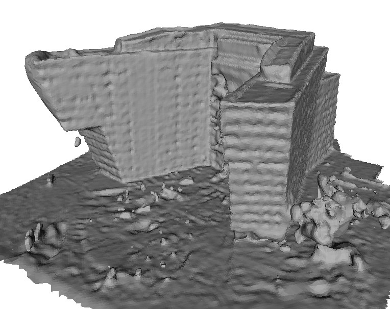
Figure 4: Models used for evaluation. Input meshes for our method obtained from image-based reconstruction.

3.2 Evaluation Metrics

As we want to know how well the computed geometry approximates the model and which degree of simplification could be achieved, we define an error measure and a regularization measure.

Error Measure. In our evaluation, we make use of an error measure which approximates the perceived error of humans by comparing the computed geometry and the ground truth model. For this, we use the Dice score [3] of the two models backprojected into all camera views. The Dice score relates the area of the two projected segments with the area of their mutual overlap. It is 1 if the two segments are completely identical and 0 if there is no overlap. To get a score for the whole model, we use the mean Dice score of all cameras. Using this measure, the 3D problem gets translated into a 2D problem consisting out of segmentation masks, which can be evaluated much easier.

Regularization Measure. As a main goal is to regularize the input data, we have to define a measure for the degree of regularization. We project the outlines of each slice (i.e., the vertical faces of the geometric model) onto the ground plane and count the number of unique lines as a complexity score. The more lines exist, the less regularized is the model.

3.3 Results

In the first row of Fig. 5 one can see results of the synthetic model with different parameter settings, the corresponding mean Dice score and the complexity measure. The Dice score and the complexity of the model are directly related to the parameter $\lambda$ and to the mean shift bandwidth. As a lesser amount of slices directly results in a big decrease of the regularization measure, models calculated with a higher bandwidth implicitly have a lower complexity score. Though, a lower mean shift bandwidth with much more smoothing can lead to the same regularization level as a higher bandwidth with lesser smoothing. More precisely, a too low bandwidth is not as critical as a too high bandwidth, as it can be compensated by a higher smoothing.

The second model used for our evaluation is a 3D model reconstructed from real-world image data and therefore includes more noise and irregularities. Further, the scene geometry is not perfectly suited for our approach as some vertical surfaces are not orthogonal to the ground plane. However, as you can see in the second row of Fig. 5, a small mean shift bandwidth leads also to an acceptable approximation of sloped structures.

In the results of both models, one can see that the incorporated noise does not have a big influence on the model quality.

For each of the resulting geometric models, we needed approximately 16 to 17 minutes of computation time on a Intel Xenon X5675 with 16 GBs RAM. However, as most of the computation time is needed for computing the free space score voxel grid, the time can be drastically reduced by using a smaller voxel grid. Further, the recomputation of results for varying values of $\lambda$ can be done within seconds.

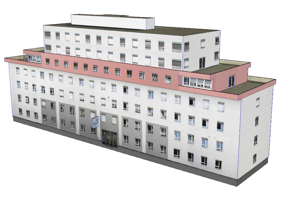
(a) Ground Truth

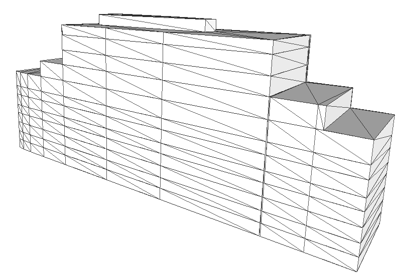
(b) $d=25$, $\lambda=4.5,\ \ \$                                                                                                                                                                    $score=0.9702$, $compl.=50$

(c) $d=10,\lambda=1.0,\ \ \$                                                                                                                                                                    $score=0.9709$, $compl.=41$

(d) $d=25,\lambda=2.5,\ \ \ \ \ \ \ \$                                                                                                                                                                    $score=0.9703$, $compl.=212$

(e) $d=35,\lambda=2.5,\ \ \ \ \ \ \ \$                                                                                                                                                                    $score=0.9770$, $compl.=472$

Figure 5: Results. In the first row, you can see geometric models created from the synthetic model and in the second row, models created from the real-world model with varying parameter settings.

4 Conclusions and Future Work

In this paper we proposed a novel approach for extracting geometric structures out of meshed point clouds reconstructed from image-based reconstruction methods. While similar techniques are used on laser scan data, we have shown that our approach can also handle noise and small irregularities due to errors in the reconstruction process.

Future work includes the detection of an optimal value for $d$ depending on the scene structure and the integration of additional scene information retrieved from the 2D images.

References

- [1] Yuri Boykov, Olga Veksler, and Ramin Zabih. Fast approximate energy minimization via graph cuts. TPAMI, 20(12):1222–1239, 2001.
- [2] Dorin Comaniciu and Peter Meer. Mean shift: A robust approach toward feature space analysis. TPAMI, 24(5):603–619, 2002.
- [3] L. R. Dice. Measures of the amount of ecologic association between species, volume 26. Ecological Society of America, 1945.
- [4] David H. Douglas and Thomas K. Peucker. Algorithms for the reduction of the number of points required to represent a digitized line or its caricature. The Canadian Cartographer, 1973.
- [5] Yasutaka Furukawa and Jean Ponce. Accurate, dense, and robust multi-view stereopsis. TPAMI, 2010.
- [6] Michael Kazhdan, Matthew Bolitho, and Hugues Hoppe. Poisson surface reconstruction. In Eurographics Symposium on Geometry Processing, 2006.
- [7] Trimble Navigation Limited and Google. Trimble 3d warehouse, 2014. http://sketchup.google.com/3dwarehouse/.
- [8] Sven Oesau, Florent Lafarge, and Pierre Alliez. Indoor scene reconstruction using primitive-driven space partitioning and graph-cut. In Eurographics Symposium on Geometry Processing, 2013.
- [9] Noah Snavely, Steven M. Seitz, and Richard Szeliski. Photo tourism: Exploring image collections in 3d. In SIGGRAPH, 2006.
- [10] Changchang Wu, Sameer Agarwal, Brian Curless, and Steven M. Seitz. Schematic surface reconstruction. In CVPR, 2012.
- [11] Jianxiong Xiao and Yasutaka Furukawa. Reconstructing the world’s museums. In ECCV, 2012.
- [12] Christopher Zach. Fast and high quality fusion of depth maps. In 3DPVT, 2008.