On the Number of Iterations for Convergence of CoSaMP and Subspace Pursuit Algorithms

Abstract

In compressive sensing, one important parameter that characterizes the various greedy recovery algorithms is the iteration bound which provides the maximum number of iterations by which the algorithm is guaranteed to converge. In this letter, we present a new iteration bound for CoSaMP by certain mathematical manipulations including formulation of appropriate sufficient conditions that ensure passage of a chosen support through the two selection stages of CoSaMP, “Augment” and “Update”. Subsequently, we extend the treatment to the subspace pursuit (SP) algorithm. The proposed iteration bounds for both CoSaMP and SP algorithms are seen to be improvements over their existing counterparts, revealing that both CoSaMP and SP algorithms converge in fewer iterations than suggested by results available in literature.

1 Introduction

Reconstruction of signals in compressed sensing (CS) [1] involves obtaining the sparsest solution to an underdetermined set of equations given as ${\bf y}={\bf A}{\bf x},$ where ${\bf A}$ is an $m\times l$ ($m<<l$) complex valued, sensing matrix and $y$ is an $m\times 1$ complex valued observation vector. It is assumed that the sparsest solution to the above system is $K$-sparse, i.e., not more than $K$ (for some minimum $K,K>0$) elements of ${\bf x}$ are non-zero and also that the sparsest solution is unique, which can be guaranteed if every $2K$ columns of $\bf A$ are linearly independent [2]. Greedy approaches like orthogonal matching pursuit (OMP) [3], compressive sampling matching pursuit (CoSaMP) [4], subspace pursuit (SP) [5], hard thresholding pursuit (HTP) [6] and others recover the $K$-sparse signal by iteratively constructing the support set of the sparse signal (i.e., index of non-zero elements in the sparse vector) by some greedy principles. These greedy pursuits are well known for their low complexity.

Convergence of these iterative procedures in a finite number of steps requires the matrix $\bf A$ to satisfy the so-called “Restricted Isometry Property (RIP)” [7] of appropriate order as given below.

Definition 1.

A matrix ${\bf A}\in\mathbb{C}^{m\times l}\;(m<l)$ is said to satisfy the RIP of order $K$ if there exists a “Restricted Isometry Constant (RIC)” $\delta_{K}\in(0,\;1)$ so that

$$(1-\delta_{K})\left|\left|{\bf x}\right|\right|_{2}^{2}\leqslant\left|\left|{\bf Ax}\right|\right|_{2}^{2}\leqslant(1+\delta_{K})\left|\left|{\bf x}\right|\right|_{2}^{2}$$ (1)

for all $K$-sparse ${\bf x}$. The constant $\delta_{K}$ is taken as the smallest number from $(0,\;1)$ for which the RIP is satisfied.

Convergence of the CS greedy recovery algorithms is usually established by imposing certain upper bounds on the RIC $\delta_{K}$ as a sufficient condition. In the case of CoSaMP, such a bound is given by $\delta_{4K}<0.5$ [8], which is a refined (i.e., more relaxed) version of two earlier bounds, namely, $\delta_{4K}<0.17157$ [4] and $\delta_{4K}<0.38427$ [9]. Similarly, for SP, the bound proposed originally is $\delta_{3K}<0.205$ [5], which was improved afterwards to $\delta_{3K}<0.325$ [10] and $\delta_{3K}<0.4859$ [8].

Apart from the convergence bound on the RIC, there is another important parameter that characterizes a greedy algorithm, namely, the iteration bound, which provides the maximum (finite) number of iterations by which the algorithm is guaranteed to converge. For CoSaMP, a signal independent iteration bound of $6(K+1)$ was presented in [4], assuming $\delta<0.1$. In this letter, we present a new iteration bound for CoSaMP which refines the above result and is given as a function of $\delta$ over the entire range for which convergence of CoSaMP is currently guaranteed (i.e., $0<\delta<0.5$). For this, we first develop a sufficient condition for capturing the support of the $p+q$ largest (in magnitude) elements of $\bf x$ within certain number of iterations ($0<p+q\leq K$), given that the support for the $p$ largest elements of $\bf x$ has already been captured. The derivation takes appropriate steps so that the above sufficient condition is obtained in a form structurally similar to the one proposed earlier for the HTP algorithm [11]. This permits computation of the iteration bound via a procedure suggested in [11]. Subsequently, we extend our approach to the SP algorithm and compute the corresponding iteration bound which is seen to be tighter than existing results on this [5] for more practical ranges of the RIC and is thus an improvement, as it establishes that the SP algorithm in more practical cases converges in fewer iterations than suggested in [5].

2 Notations and a brief review of the CoSaMP & the SP algorithms

We denote by $Z$ the index set $\{1,\,2,\cdots,\,l\}$. Then, given $B\subseteq Z$ and ${\bf z}\in\mathbb{C}^{l}$, the vector ${\bf z}_{B}\in\mathbb{C}^{l}$ is defined as follows : $[{\bf z}_{B}]_{i}=[{\bf z}]_{i}$ for $i\in B$ and $[{\bf z}_{B}]_{i}=0$ otherwise. Similarly, given the matrix ${\bf A}\in\mathbb{C}^{m\times l}$, the matrix ${\bf A}_{B}\in\mathbb{C}^{m\times l}$ is defined such that for $i\in B$, $[{\bf A}_{B}]_{i}=[{\bf A}]_{i}$ (where $[.]_{i}$ denotes the $i$-th column of the matrix $[.]$) and $[{\bf A}_{B}]_{i}={\bf 0}$ otherwise. The notation $supp(.)$ denotes the support of the vector $(.)$, i.e., $supp({\bf z})=\{i\in Z\;|\;z_{i}\neq 0\}$. By $S$ and $S^{k}$, we denote respectively the true support set of ${\bf x}$ and the estimated support set after $k$ iterations. Elements of the vector $|{\bf x}|$ sorted in descending order form the vector $\widetilde{{\bf x}}$ and the $r$-th element of $\widetilde{{\bf x}},~{}r=1,\,2,\cdots,l$ is denoted by $\widetilde{x}_{r}$, i.e., $\widetilde{x}_{r}=[\widetilde{{\bf x}}]_{r}$. The index of the $i^{th}$ largest (in magnitude) element of ${\bf x}$, $i=1,2,\cdots,|S|$ is denoted by $\pi(i)$, implying $|{\bf x}_{\pi(i)}|=\widetilde{x}_{i}$. Lastly, for a matrix $\bf A$, ${\bf A}^{h}$ denotes its Hermitian transposition.

For convenience of presentation, we adopt the convention of using the notation : $\stackrel{{\scriptstyle(.)}}{{=}}$ to indicate that the equality “$=$” follows from Equation (.) (same for inequalities). Also, unless stated otherwise, the more generalized form of CS will be considered in this paper where $\bf x$ is $K$-sparse but $\bf y$ is contaminated with a noise vector $\bf e\in\mathbb{C}^{m}$, i.e., ${\bf y}={\bf A}{\bf x}+{\bf e}$.

Table 1: Compressive Sampling Matching Pursuit algorithm

Input: measurement ${\bf y}\in\mathbb{C}^{m}$, sensing matrix ${\bf A}\in\mathbb{C}^{m\times l}$, sparsity $K$, stopping error $\epsilon$, initial estimate ${\bf x^{0}}$
For ( $n=1$ ; $||{\bf y}-{\bf A}{\bf x^{n-1}}||_{2}>\epsilon$ ; $n=n+1$ )
Identification: $\Gamma^{n}=supp(H_{2K}({\bf A}^{h}({\bf y}-{\bf A}{\bf x^{n-1}})))$
Augment: $U^{n}=S^{n-1}\cup\Gamma^{n}:S^{n-1}=supp({\bf x^{n-1}})$
Estimate: ${\bf u^{n}}=\underset{{\bf z}:supp({\bf z})=U^{n}}{\operatorname*{arg\,min}}\;||{\bf y}-{\bf A}{\bf z}||_{2}$
Update: ${\bf x^{n}}=H_{K}({\bf u^{n}})$
Output: ${\bf\hat{x}}={\bf x^{n-1}}$

The CoSaMP and the SP algorithms are given in Table LABEL:CoSaMP and LABEL:SP respectively. Both algorithms iteratively estimate $\bf x$, with ${\bf x^{n}}$ denoting the estimate at the $n$-th iteration. At the “Identification” stage, in both algorithms, the residue vector $({\bf y}-{\bf A}{\bf x^{n-1}})$ is first correlated with the columns of $\bf A$. The support $\Gamma^{n}$ of the top $r$ elements ($r=2K$ in case of CoSaMP and $r=K$ in case of SP) in terms of magnitude of correlations is then identified, using a hard thresholding operator $H_{r}(.)$ that retains the top $r$ (in magnitude) elements of the vector $(.)$ and sets other elements to zero. The vector $\bf y$ is then projected orthogonally on the column space of ${\bf A}_{S^{n-1}\cup\Gamma^{n}}$ where $S^{n-1}=supp({\bf x^{n-1}})$, generating the projection coefficient vector ${\bf u^{n}}$. In CoSaMP, the new estimate ${\bf x^{n}}$ is taken as $H_{K}({\bf u^{n}})$, whereas in SP, $\bf y$ is further projected on the column space of ${\bf A}_{S^{n}}$, where $S^{n}=supp(H_{K}({\bf u^{n}}))$, and ${\bf x^{n}}$ is taken as the corresponding projection coefficient vector.

Table 2: Subspace Pursuit Algorithm

Input: measurement ${\bf y}\in\mathbb{C}^{m}$, sensing matrix ${\bf A}\in\mathbb{C}^{m\times l}$, sparsity $K$, stopping error $\epsilon$, initial estimate ${\bf x^{0}}$
For ( $n=1$ ; $||{\bf y}-{\bf A}{\bf x^{n-1}}||_{2}>\epsilon$ ; $n=n+1$ )
Identification: $\Gamma^{n}=supp(H_{K}({\bf A}^{h}({\bf y}-{\bf A}{\bf x^{n-1}})))$
Augment: $U^{n}=S^{n-1}\cup\Gamma^{n}:S^{n-1}=supp({\bf x^{n-1}})$
Estimate: ${\bf u^{n}}=\underset{{\bf z}:supp({\bf z})=U^{n}}{\operatorname*{arg\,min}}\;||{\bf y}-{\bf A}{\bf z}||_{2}$
Update: $S^{n}=supp(H_{K}({\bf u^{n}}))$
${\bf x^{n}}=\underset{{\bf z}:supp({\bf z})=S^{n}}{\operatorname*{arg\,min}}\;||{\bf y}-{\bf A}{\bf z}||_{2}$
Output: ${\bf\hat{x}}={\bf x^{n-1}}$

3 Proposed Iteration Bound Analysis for CoSaMP and SP Algorithms

3.1 Iteration Bound for CoSaMP

The proposed iteration bound computation for CoSaMP depends on the dynamics of decay of $||{\bf x}_{\overline{U^{n}}}||_{2}$ over $n$ (under appropriate conditions on the RIC), which is presented in Lemma 1 below and is obtained by introducing suitable modifications in the corresponding analysis in [8], which considers decay of $||{\bf x}-{\bf x}^{n}||_{2}$ (rather than $||{\bf x}_{\overline{U^{n}}}||_{2}$) over $n$.

Lemma 1.

In CoSaMP algorithm, the metric $||{\bf x}_{\overline{U^{n}}}||_{2}$ decays over $n$ with the rate $\rho_{4K}=\sqrt{\frac{2\delta^{2}_{4K}(1+2\delta^{2}_{4K})}{1-\delta^{2}_{4K}}}$ as per the following :

$$||{\bf x}_{\overline{U^{n}}}||_{2}<\rho_{4K}||{\bf x}_{\overline{U^{n-1}}}||_{2}+(1-\rho_{4K})\tau\left|\left|\textbf{e}\right|\right|_{2}$$ (2)

where the constant $\tau$ is defined using $\rho_{4K}$ as, $(1-\rho_{4K})\tau=\frac{\delta_{4K}\sqrt{6(1+\delta_{3K})}}{1-\delta_{4K}}+\sqrt{2(1+\delta_{4K})}$.

Proof.

Given in Appendix A. ∎

Using the above Lemma, we next derive a sufficient condition for capturing the support of, say, the $p+q$ largest elements of $\bf x$ in $k$ iterations ($0<p+q\leq K$), assuming that the support of the $p$ largest elements of $\bf x$ has already been captured (where by “largest”, we mean largest in magnitude). In particular, we strive to obtain the above sufficient condition in a form that is structurally identical to the one developed for the HTP algorithm in Lemma 3 of [11], so that the procedure to compute the iteration bound as presented in [11] can be applied. This is, however, not easy considering that algorithmically, CoSaMP is substantially different from the HTP algorithm and is in particular characterized by certain steps like “Augment” (i.e., expansion of the support set to size $3K$, as given in Table I) and “Update” (i.e., pruning the support set to size $K$ from $3K$) not present in HTP. In Theorem 1 below, we show how the above can be achieved by deploying suitable mathematical manipulations, and in particular, by formulating appropriate sufficient conditions that ensure that the support of the $p+q$ largest elements of $\bf x$ gets selected in both the “Augment” step and the subsequent “Update” step.

Theorem 1.

Assume that at the $n$-th iteration in the CoSaMP algorithm, $S^{n}:supp({\bf x^{n}})$ contains the support of the $p~{}(p<K)$ largest (in magnitude) entries of ${\bf x}$. Then, a sufficient condition for capturing the support of the $p+q$ largest (in magnitude) entries of ${\bf x}$ in $k$ additional iterations for some integer $q$, $K-p\geq q\geq 1$ is given by

$$\widetilde{x}_{p+q}>\rho_{4K}^{k}||\widetilde{{\bf x}}_{\{p+1,p+2,\cdots,K\}}||_{2}+\gamma||e||_{2},~{}(\rho_{4K}<1)$$ (3)

where $\gamma$ is a function of $\delta_{3K}$ and $\delta_{4K}$.

Proof.

We need to ensure that the support of the largest (in magnitude) $p+q$ elements of ${\bf x}$, i.e., $\{\pi(1),\cdots,\pi(p+q)\}$ gets selected in the $(n+k)^{th}$ iteration. This means, $\pi(j),\;j\in\{1,\cdots,p+q\}$ should first belong to $U^{n+k}$, and then it also should go through the update step in CoSaMP. Now, for $\pi(j),~{}j\in\{1,\cdots,p+q\}$ to belong to $U^{n+k}$, it is sufficient to have

$$\widetilde{x}_{p+q}>||({\bf x})_{\overline{U^{n+k}}}||_{2},$$ (4)

as this ensures that the top $p+q$ elements of $\bf x$ can not belong to $({\bf x})_{\overline{U^{n+k}}}$ and thus, their support is captured in $U^{n+k}$. In order that the above support passes through the update step in CoSaMP under the satisfaction of (4), it is sufficient to have,

$$\min_{j\in\{\pi(1),\cdots,\pi(p+q)\}}{|{\bf u^{n+k}}_{j}|}>\max_{i\in U^{n+k}\setminus S}{|{\bf u^{n+k}}_{i}|}.$$ (5)

In the following, we first develop a sufficient condition (viz. (9)) which, under the satisfaction of (4), guarantees satisfaction of (5). Condition (3) is then obtained by deriving a sufficient condition for simultaneous satisfaction of (4) and (9).

Note that one can write $|{\bf u^{n+k}}_{j}|=|{\bf x}_{j}-({\bf x}_{j}-{\bf u^{n+k}}_{j})|\geq|{\bf x}_{j}|-|{\bf u^{n+k}}_{j}-{\bf x}_{j}|.$ Using this and some basic properties of inequalities, the LHS of (5) can be written as,

$$\min_{j\in\{\pi(1),\cdots,\pi(p+q)\}}{|{\bf u^{n+k}}_{j}|}$$

$$\geq\min_{j\in\{\pi(1),\cdots,\pi(p+q)\}}{|({\bf x})_{j}|-|({\bf u^{n+k}-x})_{j}|}$$

$$\geq\widetilde{x}_{p+q}-\max_{j\in\{\pi(1),\cdots,\pi(p+q)\}}|({\bf u^{n+k}-x})_{j}|,$$ (6)

while the RHS of (5) can be written as $\max_{i\in U^{n+k}\setminus S}{|{\bf u^{n+k}}_{i}|}=\max_{i\in U^{n+k}\setminus S}{|({\bf u^{n+k}}-{\bf x})_{i}|}$, since ${\bf x}_{i}=0$ for $i\in U^{n+k}\setminus S$. Combining, in order to have (5) satisfied, it is then sufficient to have,

$$\widetilde{x}_{p+q}>\max_{j\in\{\pi(1),\cdots,\pi(p+q)\}}|({\bf u^{n+k}}-{\bf x})_{j}|+\max_{i\in U^{n+k}\setminus S}{|({\bf u^{n+k}}-{\bf x})_{i}|}.$$ (7)

Now, under the satisfaction of (4), we have $\pi(j)\in U^{n+k},~{}j\in\{1,\cdots,p+q\}$. Again, $\pi(j)\in S,~{}j\in\{1,\cdots,p+q\}$. Together, these mean that $\pi(j)\in U^{n+k}\cap S,~{}j\in\{1,\cdots,p+q\}$. One can then write,

$$\max_{j\in\{\pi(1)\cdots,\pi(p+q)\}}|({\bf u^{n+k}}-{\bf x})_{j}|\leq||({\bf u^{n+k}}-{\bf x})_{U^{n+k}\cap S}||.$$

Also,

$$\max_{i\in U^{n+k}\setminus S}{|({\bf u^{n+k}}-{\bf x})_{i}|}\leq||({\bf u^{n+k}}-{\bf x})_{U^{n+k}\setminus S}||.$$

Using these and the fact that for two real numbers $a,\;b$, $a+b\leq\sqrt{2}\sqrt{a^{2}+b^{2}}$, the RHS of (7) can be written as,

$$\max_{j\in\{\pi(1),..,\pi(p+q)\}}|({\bf u^{n+k}}-{\bf x})_{j}|+\max_{i\in U^{n+k}\setminus S}{|({\bf u^{n+k}}-{\bf x})_{i}|}$$

$$<\sqrt{2}||({\bf u^{n+k}-x})_{U^{n+k}}||_{2}$$

$$\stackrel{{\scriptstyle(\ref{estimation})}}{{\leq}}\dfrac{\sqrt{2}\delta_{4K}}{\sqrt{1-\delta_{4K}^{2}}}||({\bf x})_{\overline{U^{n+k}}}||_{2}+\sqrt{2}\tau_{1}\left|\left|\textbf{e}\right|\right|_{2}.$$ (8)

From (7) and (8), it then follows that it is sufficient to have,

$$\widetilde{x}_{p+q}>\dfrac{\sqrt{2}\delta_{4K}}{\sqrt{1-\delta_{4K}^{2}}}||({\bf x})_{\overline{U^{n+k}}}||_{2}+\sqrt{2}\tau_{1}\left|\left|\textbf{e}\right|\right|_{2},$$ (9)

in order to satisfy (5) under the condition that (4) holds. Now, to satisfy both (4) and (9) simultaneously, a sufficient condition will be $\widetilde{x}_{p+q}>\max($RHS of (4), RHS of (9)$)$. Recalling that convergence of CoSaMP requires $\delta_{4K}<0.5$ [8] which implies $\dfrac{\sqrt{2}\delta_{4K}}{\sqrt{1-\delta_{4K}^{2}}}<1$, it will then be enough to have $\widetilde{x}_{p+q}>||({\bf x})_{\overline{U^{n+k}}}||_{2}+\sqrt{2}\tau_{1}\left|\left|\textbf{e}\right|\right|_{2}$ for simultaneous satisfaction of (4) and (9), where,

$$||({\bf x})_{\overline{U^{n+k}}}||_{2}+\sqrt{2}\tau_{1}\left|\left|\textbf{e}\right|\right|_{2}$$

$$\stackrel{{\scriptstyle\eqref{metric1}}}{{<}}\rho_{4K}^{k}||({\bf x})_{\overline{U^{n}}}||_{2}+(\tau+\sqrt{2}\tau_{1})\left|\left|\textbf{e}\right|\right|_{2}$$

$$\leq\rho_{4K}^{k}||({\bf x})_{\overline{S^{n}}}||_{2}+\gamma\left|\left|\textbf{e}\right|\right|_{2}$$

$$\leq\rho_{4K}^{k}||\widetilde{{\bf x}}_{\{p+1,\cdots,K\}}||_{2}+\gamma\left|\left|\textbf{e}\right|\right|_{2},$$ (10)

where $\gamma=\tau+\sqrt{2}\tau_{1}$ and the last step follows from the assumption that $S^{n}$ has captured the $p$ largest (in magnitude) elements of $\bf x$.

Hence, in order that the $p+q$ largest (in magnitude) elements of $\bf x$ get selected in $k$ additional iterations, it is sufficient to have,

$$\widetilde{x}_{p+q}>\rho_{4K}^{k}||\widetilde{{\bf x}}_{\{p+1,\cdots,K\}}||_{2}+\gamma\left|\left|\textbf{e}\right|\right|_{2}.$$ (11)

Hence proved. ∎

Note that by substituting $p=0$ and $q=K$ in Theorem 1 and taking $\left|\left|\textbf{e}\right|\right|_{2}$ to be zero, one can obtain the minimum number of iterations required to guarantee perfect recovery in the noiseless case (i.e., iteration bound), which is given by $k_{min}=\lceil\frac{{\log(\left|\left|\bf x\right|\right|_{2}}/\widetilde{x}_{K})}{\log(1/\rho_{4K})}\rceil.$ The above, however, provides a $k_{min}$ that is dependent on the signal structure, i.e., $\left|\left|\bf x\right|\right|_{2}$ and $\widetilde{x}_{K}$. A signal independent iteration bound can, however, be computed by noticing the similarity between (2) and the corresponding sufficient condition for the HTP algorithm derived in Lemma 3 of [11] (with the only difference being in the expressions for $\rho_{4K}$ and $\gamma$). To calculate $k_{min}$, one then simply has to apply the arguments used in the proof of Theorem 5 of [11] to the above context, which will require successive application of Theorem 1 on certain partitions of the index set $S$. The resulting iteration bound is given in Theorem 2 below.

Theorem 2.

With measurements ${\bf y}={\bf Ax}$, the CoSaMP algorithm converges to $\bf x$ in $\lceil cK\rceil$ number of iterations where $c=\ln{(4/\rho^{2}_{4K})}/\ln{(1/\rho^{2}_{4K})}.$

Proof.

The proof follows directly by applying the arguments used in the proof of Theorem 5 of [11] to (2) and is thus omitted. ∎

Note that unlike [4] where an iteration bound for CoSaMP was calculated assuming $0<\delta_{4K}<0.1$, the proposed bound is defined for $0<\delta_{4K}<0.5$, i.e., over the entire range for which CoSaMP is guaranteed to converge. In order to have some quantitative idea, we plot the proposed iteration bound (after normalizing by $K$) against $\delta_{4K}$ in Fig. 1. Clearly, in comparison to [4] which obtained the iteration bound as $6(K+1)$ (for $0<\delta_{4K}<0.1$), the proposed bound is about four to six times less, which is a significant improvement.

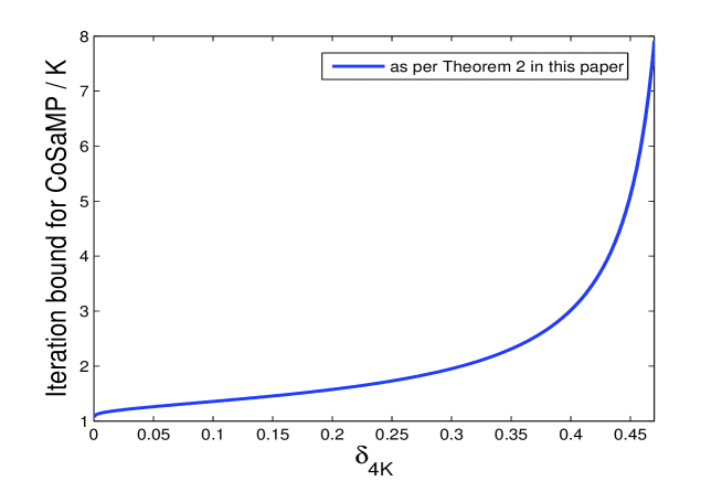
Figure 1: Dependence of the proposed iteration bound for CoSaMP (after normalizing by $K$) on the RIC $\delta_{4K}$

3.2 Extension to the Subspace Pursuit Algorithm

Like Lemma 1 for CoSaMP above, there exists a similar decay relation for the SP algorithm as well [8]. However, due to the presence of an additional orthogonal projection step in the SP algorithm (viz., the second operation in the “Update” step), the decay relation is obtained here directly in terms of $\left|\left|{\bf x}_{\overline{S^{n}}}\right|\right|_{2}$. This makes it possible to formulate a sufficient condition to capture the $p+q$ largest (in magnitude) elements of $\bf x$ within a certain number of iterations in a much simpler way than in CoSaMP and thus the derivation becomes lot simpler.

Theorem 3.

With measurements ${\bf y}={\bf Ax}$, the SP algorithm converges to ${\bf x}$ in $\lceil cK\rceil$ number of iterations, where $c=\ln{(4/\rho^{2}_{3K})}/\ln{(1/\rho^{2}_{3K})}.$

Proof.

In the SP algorithm, a decay relation analogous to Lemma 1 for CoSaMP is given by [8]

$$\left|\left|{\bf x}_{\overline{S^{n}}}\right|\right|_{2}<\rho_{3K}\left|\left|{\bf x}_{\overline{S^{n-1}}}\right|\right|_{2},$$ (12)

where $\rho_{3K}=\frac{\sqrt{2\delta_{3K}^{2}(1+\delta_{3K}^{2})}}{1-\delta_{3K}^{2}}$. As before, we now develop conditions to ensure that the support of the largest (in magnitude) $p+q$ elements of ${\bf x}$, i.e., $\{\pi(1),\cdots,\pi(p+q)\}$ get selected in $S^{n+k}$, assuming that the support $\{\pi(1),\cdots,\pi(p)\}$ has already been selected in $S^{n}$. A sufficient condition to ensure that the support $\{\pi(1),\cdots,\pi(p+q)\}$ is captured in $S^{n+k}$ will be given by,

$$\widetilde{x}_{p+q}>\left|\left|{\bf x}_{\overline{S^{n+k}}}\right|\right|_{2}.$$ (13)

From (12), proceeding recursively backwards, we can write $\left|\left|{\bf x}_{\overline{S^{n+k}}}\right|\right|_{2}<\rho_{3K}^{k}\left|\left|{\bf x}_{\overline{S^{n}}}\right|\right|_{2}$. Again, from the assumption that the support $\{\pi(1),\cdots,\pi(p)\}$ has already been selected in $S^{n}$, we have, $\left|\left|({\bf x})_{\overline{S^{n}}}\right|\right|_{2}\leq\left|\left|(\widetilde{{\bf x}})_{\{p+1,\cdots,K\}}\right|\right|_{2}$. From this and (13), a sufficient condition for ensuring that $\{\pi(1),\cdots,\pi(p+q)\}\subseteq S^{n+k}$ given that $\{\pi(1),\cdots,\pi(p)\}\subseteq S^{n}$ is given by,

$$\widetilde{x}_{p+q}>\rho_{3K}^{k}\left|\left|(\widetilde{{\bf x}})_{\{p+1,\cdots,K\}}\right|\right|_{2}.$$ (14)

Since (14) has the same form as that of Lemma 3 of [11], one can compute the iteration bound by directly applying the procedure given in Theorem 5 of [11]. The resulting iteration bound is given by $\lceil cK\rceil$, where $c=\frac{\ln{(4/\rho^{2}_{3K})}}{\ln{(1/\rho^{2}_{3K})}}$. ∎

For higher and thus more practical values of $\delta_{3K}$, the iteration bound proposed in Theorem 3 is an improvement over the existing result $\lceil\frac{1.5K}{\ln{(1/\rho_{3K})}}\rceil$ as given in Theorem 6 of [5]. To show this, we plot both the iteration bounds (after normalizing by $K$) against $\delta_{3K}$ in Fig. 2 over the range $0<\delta_{3K}<0.4859$, i.e., the range for which the SP algorithm is guaranteed to converge, after adopting $\rho_{3K}$ from [8]. It is seen from Fig. 2 that while for $0<\delta_{3K}<0.28$, the proposed iteration bound is slightly higher than that of [5], for $\delta_{3K}>0.28$ (which is also a more practical range for $\delta_{3K}$ for the SP algorithm), the former is significantly lesser than the latter and the difference grows with $\delta_{3K}$. This shows that for more practical ranges of $\delta_{3K}$, the SP algorithm actually converges in significantly fewer iterations than suggested in [5].

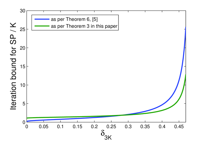
Figure 2: Comparison of the proposed iteration bound of the SP algorithm vis-a-vis the existing iteration bound as given in [5].

Appendix A Proof of Lemma 1

As a consequence of the identification step in CoSaMP, as proved in Lemma 7, [8], we can write,

$$\left|\left|({\bf x})_{\overline{U^{n}}}\right|\right|_{2}\leq\sqrt{2}\delta_{4K}\left|\left|{\bf x}-{\bf x^{n-1}}\right|\right|_{2}+\sqrt{2(1+\delta_{4K})}\left|\left|\textbf{e}\right|\right|_{2},$$ (15)

Now, we need to upper bound $\left|\left|{\bf x}-{\bf x^{n-1}}\right|\right|_{2}$ in terms of $\left|\left|({\bf x})_{\overline{U^{n-1}}}\right|\right|_{2}$. For notational convenience, we obtain the upper bound of $\left|\left|{\bf x}-{\bf x^{n}}\right|\right|_{2}$ in terms of $\left|\left|({\bf x})_{\overline{U^{n}}}\right|\right|_{2}$ and then replace $n$ with $n-1$ later. For this, the estimation step of CoSaMP is analyzed next. For any ${\bf z}\in\mathbb{C}^{l\times 1}$ with $supp({\bf z})\subseteq U^{n}$, the estimation step in CoSaMP ensures that $\langle{\bf y}-{\bf Au^{n}},{\bf Az}\rangle=0$. Substituting $\bf y$ by ${\bf A}{\bf x}+{\bf e}$, this leads to $\langle{\bf u^{n}}-{\bf x},{\bf A}^{h}{\bf Az}\rangle=\langle{\bf e},{\bf Az}\rangle$. Defining $V^{n}=U^{n}\cup S$, this can also be written as,

$$\langle{\bf u^{n}}-{\bf x},{\bf A}^{h}_{V^{n}}{\bf A}_{V^{n}}{\bf z}\rangle=\langle{\bf e},{\bf A}{\bf z}\rangle.$$ (16)

Taking $z=({\bf u^{n}}-{\bf x})_{U^{n}}$, one then obtains,

$$||({\bf u^{n}}-{\bf x})_{U^{n}}||_{2}^{2}=\langle{\bf u^{n}}-{\bf x},({\bf u^{n}}-{\bf x})_{U^{n}}\rangle,$$

$$\stackrel{{\scriptstyle(\ref{estimation1})}}{{=}}\langle{\bf u}^{n}-{\bf x},(I-{\bf A}^{h}_{V^{n}}{\bf A}_{V^{n}})({\bf u^{n}}-{\bf x})_{U^{n}}\rangle+\langle{\bf e},{\bf A}({\bf u^{n}}-{\bf x})_{U^{n}}\rangle,$$

$$\leq\delta_{4K}||{\bf u^{n}}-{\bf x}||_{2}||({\bf u^{n}}-{\bf x})_{U^{n}}||_{2}+\sqrt{1+\delta_{3K}}||{\bf e}||_{2}||({\bf u^{n}}-{\bf x})_{U^{n}}||_{2},$$ (17)

where (17) follows from consequences of RIP as presented in Lemma 1,2 [8]. With $A=||({\bf u^{n}}-{\bf x})_{U^{n}}||_{2}$, $B=||({\bf u^{n}}-{\bf x})_{\overline{U^{n}}}||_{2}$ and $||{\bf u^{n}}-{\bf x}||_{2}^{2}=A^{2}+B^{2}$, (17) can be reduced to $A\leq\delta_{4K}\sqrt{A^{2}+B^{2}}+\sqrt{1+\delta_{3K}}||{\bf e}||_{2}$. After solving the above quadratic equation in $A$ with appropriate inequalities, we get,

$$||({\bf u^{n}}-{\bf x})_{U^{n}}||_{2}\leq\dfrac{\delta_{4K}}{\sqrt{1-\delta_{4K}^{2}}}||({\bf u^{n}}-{\bf x})_{\overline{U^{n}}}||_{2}+\tau_{1}\left|\left|\textbf{e}\right|\right|_{2},$$ (18)

where $\tau_{1}=\dfrac{\sqrt{1+\delta_{3K}}}{1-\delta_{4K}}$. Coming to the update step, as $S^{n}$ is the best $K$ term approximation to $U^{n}$, we can say

$$\left|\left|{\bf u^{n}}_{A\setminus B}\right|\right|_{2}\leq\left|\left|{\bf u^{n}}_{B\setminus A}\right|\right|_{2}=\left|\left|({\bf u^{n}}-{\bf x})_{B\setminus A}\right|\right|_{2},$$ (19)

where $A=U^{n}\setminus S^{n}$ and $B=U^{n}\setminus S$. We also have,

$$\left|\left|{\bf u^{n}}_{A\setminus B}\right|\right|_{2}=\left|\left|({\bf u^{n}}-{\bf x})_{A\setminus B}+({\bf x})_{A}\right|\right|_{2}$$ (20)

$$\geq\left|\left|({\bf x})_{U^{n}\setminus S^{n}}\right|\right|_{2}-\left|\left|({\bf u^{n}}-{\bf x})_{A\setminus B}\right|\right|_{2}.$$ (21)

From (19) and (21), we get,

$$\left|\left|({\bf x})_{U^{n}\setminus S^{n}}\right|\right|_{2}\leq\sqrt{2}\left|\left|({\bf u^{n}}-{\bf x})_{A\cup B}\right|\right|_{2}\leq\sqrt{2}\left|\left|({\bf u^{n}}-{\bf x})_{U^{n}}\right|\right|_{2}.$$ (22)

Finally, we can upper bound $\left|\left|{\bf x}-{\bf x^{n}}\right|\right|_{2}$ as,

$$\left|\left|{\bf x}-{\bf x^{n}}\right|\right|_{2}^{2}=\left|\left|({\bf x}-{\bf x^{n}})_{S^{n}}\right|\right|_{2}^{2}+\left|\left|({\bf x}-{\bf x^{n}})_{\overline{S^{n}}}\right|\right|_{2}^{2}$$

$$=\left|\left|({\bf x}-{\bf x^{n}})_{S^{n}}\right|\right|_{2}^{2}+\left|\left|({\bf x})_{\overline{U^{n}}}\right|\right|_{2}^{2}+\left|\left|({\bf x})_{U^{n}\setminus S^{n}}\right|\right|_{2}^{2}$$

$$\stackrel{{\scriptstyle(\ref{update})}}{{\leq}}\left|\left|({\bf x}-{\bf x^{n}})_{S^{n}}\right|\right|_{2}^{2}+\left|\left|({\bf x})_{\overline{U^{n}}}\right|\right|_{2}^{2}+2\left|\left|({\bf u^{n}}-{\bf x})_{U^{n}}\right|\right|_{2}^{2}$$

$$\leq 3\left|\left|({\bf x}-{\bf u^{n}})_{U^{n}}\right|\right|_{2}^{2}+\left|\left|({\bf x})_{\overline{U^{n}}}\right|\right|_{2}^{2}$$

$$\stackrel{{\scriptstyle(\ref{estimation})}}{{\leq}}\big{(}\dfrac{\sqrt{3}\delta_{4K}}{\sqrt{1-\delta_{4K}^{2}}}\left|\left|({\bf x})_{\overline{U^{n}}}\right|\right|_{2}+\sqrt{3}\tau_{1}\left|\left|\textbf{e}\right|\right|_{2}\big{)}^{2}+\left|\left|({\bf x})_{\overline{U^{n}}}\right|\right|_{2}^{2}$$

$$\leq(\sqrt{\dfrac{1+2\delta_{4K}^{2}}{1-\delta_{4K}^{2}}}\left|\left|({\bf x})_{\overline{U^{n}}}\right|\right|_{2}+\sqrt{3}\tau_{1}\left|\left|\textbf{e}\right|\right|_{2})^{2}.$$ (23)

Using (23) with (15), we then arrive at the result.

Comment : Lemma 1 and its proof as given above has some important differences with its counterpart presented in [8] (i.e., Theorem 2 of [8]). In [8], a similar decay relation was presented in terms of $\left|\left|{\bf x}-{\bf x^{n}}\right|\right|_{2}$. For this, $\left|\left|({\bf x}-{\bf x^{n}})_{S^{n}}\right|\right|_{2}$ and $\left|\left|({\bf x}-{\bf x^{n}})_{\overline{S^{n}}}\right|\right|_{2}$ were separately upper bounded by $\left|\left|{\bf x}-{\bf x^{n-1}}\right|\right|_{2}$, and then the results were combined to obtain an upper bound of

$$\left|\left|{\bf x}-{\bf x}^{n}\right|\right|_{2}=\sqrt{\left|\left|({\bf x}-{\bf x^{n}})_{S^{n}}\right|\right|_{2}^{2}+\left|\left|({\bf x}-{\bf x^{n}})_{\overline{S^{n}}}\right|\right|_{2}^{2}}$$

in terms of $\left|\left|{\bf x}-{\bf x^{n-1}}\right|\right|_{2}$. In contrast, in our treatment here, we try to upper bound $\left|\left|({\bf x})_{\overline{U^{n}}}\right|\right|_{2}$ in terms of $\left|\left|({\bf x})_{\overline{U^{n-1}}}\right|\right|_{2}$, for which we first obtain an upper bound of $\left|\left|{\bf x}-{\bf x^{n}}\right|\right|_{2}$ in terms of $\left|\left|({\bf x})_{\overline{U^{n}}}\right|\right|_{2}$ (i.e., (23)) and subsequently combine it with (15) (with $n$ replaced by $(n-1)$ in (23)). Interestingly, in doing so, we can obtain a decay relation of the metric $\left|\left|{\bf x}-{\bf x^{n}}\right|\right|_{2}$ by combining (23) with (15), given as

$$\left|\left|{\bf x}-{\bf x^{n}}\right|\right|_{2}\leq\rho_{4K}\left|\left|{\bf x}-{\bf x^{n-1}}\right|\right|_{2}+(1-\rho_{4K})\alpha\left|\left|\textbf{e}\right|\right|_{2},$$ (24)

where $(1-\rho_{4K})\alpha=\frac{\sqrt{3(1+\delta_{3K})}}{1-\delta_{4K}}+\sqrt{\frac{2(1+\delta_{4K})(1+2\delta_{4K}^{2})}{1-\delta_{4K}^{2}}}$. The relation (24) is almost identical to the decay relation given in Theorem 2 of [8], with the only difference being that the coefficient $(1-\rho_{4K})\alpha$ in (24) is lesser than the corresponding coefficient in [8] as can be verified trivially. For example, with $\rho_{4K}=0.5$ (meaning $\delta_{4K}\approx 0.3$), $\alpha\approx 9.4$ in (24), whereas $\alpha\approx 13.7$ in Theorem 2 of [8].

References

- [1] D.L. Donoho, “Compressed sensing”, IEEE Trans. Information Theory, vol. 52, no. 4, pp. 1289-1306, Apr., 2006.
- [2] J. A. Tropp and S. J. Wright, “Computational methods for sparse solution of linear inverse problems,” Proc. IEEE, vol. 98, no. 6, pp. 948-958, June, 2010.
- [3] J.A. Tropp, and A.C. Gilbert, “Signal recovery from random measurements via orthogonal matching pursuit”, IEEE Trans. Information Theory, vol. 53, no. 12, pp. 4655-4666, Dec., 2007.
- [4] D. Needell and J. Tropp, “CoSaMP : Iterative Signal Recovery from Incomplete and Inaccurate Samples”, Appl. Comput. Harmon. Anal., vol. 26, pp. 301-321, 2009; also, ACM Technical Report 2008-01, California Institute of Technology, Pasadena, July 2008.
- [5] W. Dai and O. Milenkovic, “Subspace Pursuit for Compressive Sensing Signal Reconstruction”, IEEE Trans. Information Theory, vol. 55, no. 5, pp. 2230-2249, 2009.
- [6] S. Foucart, “Hard Thresholding Pursuit: An Algorithm for Compressive Sensing”, SIAM J. Numer. Anal., vol. 49, no. 6, pp. 2543-2563, 2011.
- [7] M. Elad, Sparse and Redundant Representations, Springer, 2010.
- [8] C. B. Song, S. T. Xia, X. J. Liu, “Improved Analyses for SP and CoSaMP Algorithms in Terms of Restricted Isometry Constants”, arXiv:1309.6073, Sept. 2013.
- [9] Foucart, Simon, “Sparse Recovery Algorithms: Sufficient Conditions in Terms of Restricted Isometry Constants”, Approximation Theory XIII: San Antonio 2010, Springer Proceedings in Mathematics , vol. 13, pp. 65-77, 2012.
- [10] Kiryung Lee; Bresler, Y.; Junge, M., “Oblique Pursuits for Compressed Sensing,” IEEE Trans. Information Theory, vol. 59, no. 9, pp. 6111-6141, Sept. 2013.
- [11] J.-L. Bouchot, S. Foucart, P. Hitczenko, “Hard thresholding pursuit algorithms: number of iterations”, preprint, url: http://www.math.uga.edu/ foucart/HTPbis.pdf