Unified Structured Learning for Simultaneous Human Pose Estimation and Garment Attribute Classification

Abstract

In this paper, we utilize structured learning to simultaneously address two intertwined problems: 1) human pose estimation (HPE) and 2) garment attribute classification (GAC), which are valuable for a variety of computer vision and multimedia applications. Unlike previous works that usually handle the two problems separately, our approach aims to produce an optimal joint estimation for both HPE and GAC via a unified inference procedure. To this end, we adopt a preprocessing step to detect potential human parts from each image (i.e., a set of “candidates”) that allows us to have a manageable input space. In this way, the simultaneous inference of HPE and GAC is converted to a structured learning problem, where the inputs are the collections of candidate ensembles, the outputs are the joint labels of human parts and garment attributes, and the joint feature representation involves various cues such as pose-specific features, garment-specific features, and cross-task features that encode correlations between human parts and garment attributes. Furthermore, we explore the “strong edge” evidence around the potential human parts so as to derive more powerful representations for oriented human parts. Such evidences can be seamlessly integrated into our structured learning model as a kind of energy function, and the learning process could be performed by standard structured Support Vector Machines (SVM) algorithm. However, the joint structure of the two problems is a cyclic graph, which hinders efficient inference. To resolve this issue, we compute instead approximate optima by using an iterative procedure, where in each iteration the variables of one problem are fixed. In this way, satisfactory solutions can be efficiently computed by dynamic programming. Experimental results on two benchmark datasets show the state-of-the-art performance of our approach.

I Introduction

Human-oriented technologies play important roles in many computer vision and multimedia applications that require interactions between persons and electronic devices. The significance of human-oriented technologies naturally drives the research community to extensively investigate human-related topics, such as face recognition [1], human tracking [2], pose estimation [3], clothing technology [4], etc. In this work, we are interested in two of them: human pose estimation (HPE) and clothing technology (CT). Both problems have been studied extensively, and a review of previous work is presented in the following section.

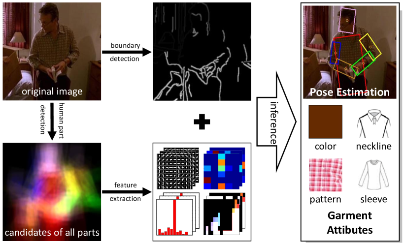
Figure 1: Overview of the proposed approach. For a given image, first we detect candidates that have potentials to be valid human parts using the HPE algorithm proposed in [3]. This preprocessing step simplifies the representation of the image and converts the joint inference of HPE and GAC into a structured learning problem. Second, we design the joint feature representation for structured learning using various visual cues. Meanwhile, potential strong edges in the image are detected by utilizing a well-established algorithm presented in [5]. Finally, we use the prediction function learned from structured SVM to produce the joint labels of human parts and garment attributes.

I-A Previous Work

I-A1 Human Pose Estimation

The literature about HPE can trace back to 40 years ago. Fischler and Elschlager [6] proposed to represent the articulated human pose as a collection of rigid body parts. This classical model, called pictorial structure (PS) in [7], provides a straightforward representation for articulated objects and owns a tree structure that can facilitate efficient inference. Hence, PS is still adopted as a basic tool by recently established approaches, e.g., [8, 9, 10, 11, 12, 13]. These recent works mainly pursue better feature description, more efficient computation, more complex human structures and more effective contextual information.

Feature description is one of the key elements for various vision tasks and so HPE [14]. In [12], an iterative parsing paradigm was introduced to obtain an increasingly finer feature scheme for describing human parts. Other works, e.g., [8, 10], employed shape-based feature descriptors such as Shape Context [15] and Histogram of Oriented Gradients (HOG) [16], which proved to be more effective than color-based features. In [9], Eichner and Ferrari considered the appearance consistence between connected/symmetric limbs and developed a better appearance model.

The majority of early works on HPE emphasized on detection performance, i.e., a more effective inference schema, and the focus of later works was placed on the efficiency of inference. Typically, the search space of human pose is the main bottleneck for improving the efficiency, because one must search over the location and orientation space for each human part, as well as over the image pyramid. To reduce the search space of human poses, Ferrari et al. [11] utilized a generic upper-body detector and the GrabCut [17] algorithm, targeting at a reduced search space. In [8, 18, 19], the tree structure is used to make the inference procedure more efficient, which can also well handle the spatial association between different human parts. One advantage of the tree structure is the ability to allow a fast computation via a dynamic programming [7]. Furthermore, deformable cost computation between connected human parts can be accelerated by performing a distance transform if the pair-wise cost suffices some specific conditions [7].

Although the tree-based PS models can draw a general representation for human body, it does not explore the implicit connections between rigid parts that do not share joints [20]. Therefore, graph-based structures are further proposed and explored by recent works. Such models are hard to be learnt exactly because of their high computational cost over the graph structure. Usually, Markov Random Filed (MRF) is used to achieve an approximate inference. By taking a branch and bound step in [20], inference on a graph is nearly as efficient as the tree models. Recently, Yang and Ramanan [3] proposed a method that represents each human part by a mixture of templates. Unlike the previous limb models with articulated orientations, their templates are non-oriented and can well capture near-vertical and near-horizontal limbs. By tuning the part type and location, their model can handle the in-plane rotation and foreshortening.

Another drawback of the original PS model is that the contextual information is not explicitly considered. In the work of Sapp et al. [19], various visual cues (e.g., boundary and segmentation) were employed in their coarse-to-fine model. In [13], Rothrock et al. incorporated background context into the PS model. Their model encourages a high contrast of a part region from its surroundings. Experimental results in their paper demonstrated the effectiveness of such contextual information.

I-A2 Clothing Technology

The clothing technologies, mainly including clothing segmentation [21, 22, 23], clothing recommendation [24] and garment attribute classification [4], play an important role in many multimedia systems such as clothing search engines [25], online shopping [26] and human recognition [27].

The work of Chen et al. [28] is one of the representative works in the related literature, which introduced an And-Or graph to generate a large set of composite clothing components for further recognition. In [26], Liu et al. proposed a cross-scenario clothing retrieval system which can search similar garments from the online shop by using a person’s daily life photo as input. In their work, a well trained human part detector was employed for part alignment and an offline transfer learning scheme was introduced to handle the discrepancy between images from daily life and online shops. Recently, they proposed a practical system called “magic closet” in [24] which can automatically recommend garments according to occasions. They utilized the latent SVM algorithm and modeled the clothing attributes as latent variables to provide mid-level features, rather than directly bridging the raw image features to the occasions.

Recent progress in clothing techniques has witnessed the benefit of HPE due to the strong relations between human parts and garment attributes. In other words, it is a popular way to perform clothing study based on the results of human part detection [4, 26]. Moreover, Yamaguchi et al. [23] and Chen et al. [4] used well trained human part detectors to produce a large number of garment types, aiming to achieve precise clothing recognition. Bourdev et al. [29] trained an SVM classifier over each human part with the purpose of indicating whether or not a human part has specific garment attributes.

I-A3 HPE and CT

There are few works addressing the interrelations between HPE and CT. Yamaguchi et al. [23] tried to refine both HPE and clothing parsing by using a three-stage scheme: first, they obtained some initial results of HPE; second, they used those initial HPE results as the basis to gain more reliable clothing segmentation; finally, the produced segmentation results were used to further refine HPE. However, since the quality of clothing segmentation largely depends on the success of HPE and vice versa, such a separate modeling approach may fail to capture the correlations between the two tasks and cannot achieve significant improvements over the competing baseline, as can be seen from the reports in [23]. In the recent work of Ladicky et al. [30], they combined the part-based approach of pose estimation and pixel-based approach of image labeling into a principle way so as to inherit advantages of both. Inference for their model was performed with two steps: first, they iteratively added the next best pose candidate by computing an energy function of their model; second, they refined the final solution over the selected candidates of the first step.

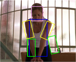
(a)

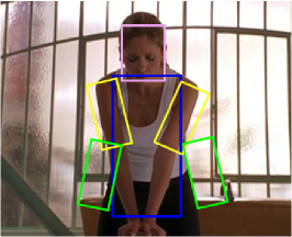
(b)

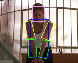
(c)

Figure 2: Examples to illustrate that GAC can help HPE. (a) Result with incorrect left-lower arm. (b) Result with both incorrect lower arms. (c) Result with all correct arms. For (a), one can immediately assert that the HPE result can hardly be correct because the appearances of right-lower arm and left-lower arm differ greatly. Such prior knowledge about limb appearance was considered in [9]. However, it can’t distinguish which human estimation is right from (b) and (c) in this way, where the lower arms’ appearances differ slightly. Given that the garment attribute is known, e.g., sleeve type is sleeveless, one can easily exclude (b) because the lower arms in (b) have few skin colors.

I-B Contributions of This Work

It is indeed natural to anticipate that HPE and CT are intertwined problems and can help each other. For example, in Figure 2, depending on the garment type, one can erase a large number of incorrect HPE candidates. However, existing approaches that individually use pose information to refine CT or use clothing knowledge to help HPE cannot fully capture the advantages of modeling the correlations between the two tasks. In this paper, we therefore propose to integrate HPE and garment attribute classification (GAC) into a unified framework, with the purpose of making effective use of the possible correlations between human parts and garment attributes.

Also, we aim to provide an effective way to jointly model multiple visual cues, including the features specific for human parts (pose-specific features) and for garment attributes (garment-specific features), as well as the cross-task features that encode the correlations between human parts and garment attributes. For a more informative description for oriented human part, we explore the “strong edge” evidence as an energy function so as to incorporate the contextual information around a human part. This motivation is based on the following observation: Since our representation for a human part is an oriented bounding box, it generally holds that there exist parallel edges sharing a similar orientation with an underlying correct part candidate, as illustrated in Figure 5.

To this end, we use the HPE algorithm presented in [3] to obtain from each image a set of bounding boxes (called “candidates”) that have potentials to be correct human parts, resulting in a basic representation for each image – one image is represented by one set of candidate ensembles. In this way, the joint inference for HPE and GAC is converted to a structured learning [31] problem, where the input is the image represented by a collection of candidate ensembles, the output is the joint labels of human parts and garment attributes, and the joint feature representation involves the aforementioned multiple visual cues.

Given a set of annotated training images, the prediction function of structured learning is learnt by using the structured Support Vector Machines (SVM) algorithm. Inference for a new test samples can be performed efficiently by iteratively computing a local optimum on a tree with the dynamic programming algorithm. Experimental results on two benchmark datasets show the state-of-the-art performance of our approach.

One may want to take HPE and GAC into the multi-task learning (MTL) framework [32]. We remark here that our problem cannot be solved via existing MTL methods since models of MTL always assume that the underlying tasks share the same feature space. In our case, however, this assumption is not valid as we address two different tasks: human pose estimation (a detection task) and garment attribute classification (a recognition task). Each of the two tasks has its own feature space that can not be shared with the other, i.e. pose-specific features and garment specific features (see Section II-B). Also, methods from domain adaption (DA) [33] cannot be applied as DA algorithms deal with the variations in some combinations of factors, including scene, object location and pose, view angle, resolution etc. Obviously, our problem is not under the setting of DA algorithms.

The rest of the paper is organized as follows. Section II elaborates on our approach for combined HPE and GAC, including feature design, parameter learning and inference algorithm. Section III presents the experiments and results. Section IV concludes this paper and discusses our future work.

II Joint Inference of HPE and GAC

As Figure 1 shows, our approach contains three major procedures, including a preprocessing step that detects candidates from each image, an engineering step that forms a joint feature representation from various visual cues, and an inference step that uses structured SVM learned from a set of training images. In the following, we shall detail each step one by one.

II-A Preprocessing and Problem Formulation

We do not build our approach by directly utilizing the images represented by raw pixels, and instead, we use the existing HPE method [3] to produce some initial results as input to our approach. More precisely, for each human part $i$ (e.g., head), we perform a non-maximum suppression on the output of [3] and take the top $K_{i}$ (each $K_{i}=40$ in our work) candidates (denoted by $\mathbf{b}_{i}$) from each image, where each candidate is a bounding box $(x,y,\theta,s)$, with $(x,y)$, $\theta$ and $s$ denoting the center coordinates, the angle and the size of the bounding box, respectively . This step allows us to obtain a manageably sized state space and simplifies the representation of a given instance. Suppose there are $m$ human parts in total ($m=6$ in this work), and then each image is represented by $m$ candidate ensembles, each of which contains $K_{i}$ candidates respectively. Thus, the input space (i.e., sample space) $\mathcal{X}$ of our approach is defined as

$$\mathcal{X}=\{\mathbf{x}\mid\mathbf{x}=(\mathbf{b}_{1},\mathbf{b}_{2},\cdots,\mathbf{b}_{m})\},$$ (1)

where $\mathbf{x}$ refers to an image and $\mathbf{b}_{i}$ denotes the candidate ensemble for the $i$-th human part (there are $K_{i}$ candidates in $\mathbf{b}_{i}$). Furthermore, we introduce the following notation:

$$\mathcal{P}=\{\mathbf{p}\mid\mathbf{p}=(p_{1},p_{2},\cdots,p_{m}),\forall i,1\leq p_{i}\leq K_{i}\},$$ (2)

where $p_{i}$ is a positive integer that indicates the index of the candidate for the $i$-th human part. In this way, the task of HPE is formulated as the problem of learning a prediction function from $\mathcal{X}$ to $\mathcal{P}$.

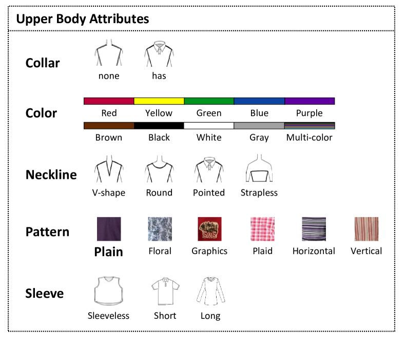
Figure 3: Garment attributes definition. We list all the garment attributes and types. In this work, we focus on the upper body dressing style. Part of the icons in this figure are quoted from [26].

TABLE I: the interdependency between human parts and garment attributes. first column: a garment attribute; second column: the human parts associating with the garment attribute shown in the first column; third column: the corresponding feature descriptors used to describe the parts (or attribute).

Attribute	Human Parts	Low-level Features
Collar	Torso$+$Head	HOG
Color	Torso	Color Histogram
Neckline	Torso$+$Head	HOG
Pattern	Torso	LBP [34]
Sleeve	All arms	Color Histogram

The goal of GAC in our work is to determine the garment attributes possessed by each image. We consider five types of attributes, including “Collar”, “Color”, “Neckline”, “Pattern” and “Sleeve” that are most relevant with the upper body limbs. Each attribute has multiple styles, e.g., short sleeve and long sleeve for the “Sleeve” attribute. We use $T_{k}$ to denote the number of attribute values for the $k$-th attribute. The attribute values we consider in this paper are given in Figure 3. For the ease of presentation, we introduce the following notation:

$$\mathcal{C}=\{\mathbf{c}\mid\mathbf{c}=(c_{1},c_{2},\cdots,c_{n}),\forall k,1\leq c_{k}\leq T_{k}\},$$ (3)

where $n$ is the number of garment attributes ($n=5$ in this work), and $c_{k}$ is the label for the $k$-th attribute (e.g., $c_{5}=1$ means short sleeve, and $c_{5}=2$ means long sleeve). In this way, similar with HPE, the task of GAC can also be formulated as a problem of learning a prediction function from $\mathcal{X}$ to $\mathcal{C}$.

Hence, the task of performing combined HPE and GAC can be formulated as follows:

$$f:\mathcal{X}\rightarrow\mathcal{Y},$$ (4)

where $\mathcal{Y}$ is the joint output space defined by

$$\mathcal{Y}=\{\mathbf{y}\mid\mathbf{y}=(\mathbf{p},\mathbf{c}),\mathbf{p}\in\mathcal{P},\mathbf{c}\in\mathcal{C}\}.$$ (5)

Regarding the prediction function $f$, we first presume that there is a compatibility function $S$ that measures the fitness between an input-output pair $(\mathbf{x},\mathbf{y})$:

$$S(\mathbf{x},\mathbf{y};\mathbf{w})=\mathbf{w}\cdot J(\mathbf{x},\mathbf{y})+\alpha Q(\mathbf{x},\mathbf{p}),$$ (6)

where $\mathbf{w}\cdot J(\mathbf{x},\mathbf{y})$ denotes the inner product of two vectors, $J(\mathbf{x},\mathbf{y})$ is the joint feature representation (which should be designed carefully), $\mathbf{w}$ is an unknown weight vector (which should be learned from training samples), $Q(\mathbf{x},\mathbf{p})$ is the energy function indicating the response of a strong edge around the potential human parts and $\alpha$ is a parameter (which can be hand-tuned by cross-validation).

In this way, the mapping function $f$ in Eq. (4) can be written as:

$$f(\mathbf{x};\mathbf{w})=\operatorname*{arg\,max}_{\mathbf{y}\in\mathcal{Y}}S(\mathbf{x},\mathbf{y};\mathbf{w}).$$ (7)

II-B Joint Feature Representation

The joint feature representation $J(\mathbf{x},\mathbf{y})$ is an important component of the prediction function. In our approach, $J(\mathbf{x},\mathbf{y})$ consists of three types of features, including the pose-specific features denoted by $J_{p}(\mathbf{x},\mathbf{p})$, the garment-specific features denoted by $J_{c}(\mathbf{c})$, and the cross-task features denoted by $J_{pc}(\mathbf{x},\mathbf{y})$; that is,

$$\mathbf{w}\cdot J(\mathbf{x},\mathbf{y})=\mathbf{w}_{p}\cdot J_{p}(\mathbf{x},\mathbf{p})+\mathbf{w}_{c}\cdot J_{c}(\mathbf{c})+\mathbf{w}_{pc}\cdot J_{pc}(\mathbf{x},\mathbf{y}).$$ (8)

In the following, we shall present our techniques used to design each type of feature.

II-B1 Pose-Specific Features

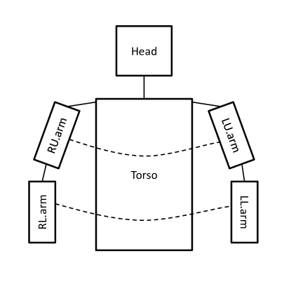
Figure 4: Part-part relations. The solid lines are used to indicate spatially connected parts, e.g., torso and right upper arm (RU.arm). We mainly consider the geometry constraint for this case, e.g., relative position and relative rotation. The dashed lines mean the relations between symmetric parts, e.g., right upper arm (RU.arm) and left upper arm (LU.arm). For these parts, we model the appearance constraint, i.e., appearance similarity in color and texture descriptors.

Given an image represented as $m$ candidate ensembles (each candidate is a bounding box), we extract some features specifically useful for HPE, called pose-specific features, as follows:

$$\begin{split}\mathbf{w}_{p}\cdot J_{p}(\mathbf{x},\mathbf{p})=&\sum_{i=1}^{m}\mathbf{w}_{p}^{u,i}\cdot\phi_{p}(\mathbf{x},p_{i})\\ &+\sum_{(i,j)\in E_{p}^{d}}\mathbf{w}_{p}^{d,ij}\cdot\psi_{p}^{d}(\mathbf{x},p_{i},p_{j})\\ &+\sum_{(i,j)\in E_{p}^{c}}\mathbf{w}_{p}^{c,ij}\cdot\psi_{p}^{c}(\mathbf{x},p_{i},p_{j}),\end{split}$$ (9)

where $\phi_{p}(\mathbf{x},p_{i})$ denotes the unary feature for the $i$-th human part, $\psi_{p}^{d}(\mathbf{x},p_{i},p_{j})$ models the pairwise relations between spatially connected human parts, $E_{p}^{d}$ is the collection of all pairs of connected parts, $\psi_{p}^{c}(\mathbf{x},p_{i},p_{j})$ contains the appearance consistency message between symmetric parts and $E_{p}^{c}$ is the set of all symmetric parts (see Figure 4 for details). The three terms are called unary score, deformation score and consistency score respectively.

In our approach, the unary feature $\phi_{p}(\mathbf{x},p_{i})$ is chosen as the HOG descriptor [16] which has been proved quite effective for object detection [10, 3].

The design of $\psi_{p}^{d}(\mathbf{x},p_{i},p_{j})$ concerns some basic geometry constraints between connected parts, including relative position, rotation and distance of part candidate $p_{i}$ with respect to $p_{j}$. More concretely, we divide the image space into 3 by 3 regions, with $p_{j}$ at the central region. Then we use a $9$ dimensional one-zero vector as the relative position feature, where there is only one element with value “1” that indicates the region where $p_{i}$ is located. To describe the relative rotation, we divide the range of angles $[0,360]$ into 20 bins and use a $20$ dimensional one-zero vector as the feature. Our relative distance feature is the euclidean distance between the center of $p_{i}$ and $p_{j}$.

For the symmetric parts, we assume some consistency constraints between them which hold for most cases; that is, they should share similar appearance. In this work, we compute the divergence of the color histogram in RGB and LAB space and take it as the feature descriptors.

In Figure 4, we mark all the parts that are related to each other.

II-B2 Garment-Specific Features

There are some features only specific for garment, i.e., garment-specific features. In this work, we consider the co-occurrences between different garment attribute values:

$$\mathbf{w}_{c}\cdot J_{c}(\mathbf{c})=\sum_{k,l}\mathbf{w}_{c}^{kl}\cdot\psi_{c}(c_{k},c_{l}),$$ (10)

where $\psi_{c}(c_{k},c_{l})$ is a binary vector that indicates whether or not $c_{k}$ and $c_{l}$ co-occur in an image. For example, the texture type “drawing” (usually belongs to T-shirt style) often co-occurs with the collar type “round”.

II-B3 Cross-Task Features

The cross-task features encode the correlations between human parts and garment attributes. In our approach, we model the part-garment relations manually specified as in Table I. For a given attribute $k$, we denote the human part(s) associated with it as $\hat{\mathbf{p}}(k)$ and the corresponding configuration(s) as $\hat{\mathbf{p}}_{k}$. Then the cross-task features are formulated as:

$$\mathbf{w}_{pc}\cdot J_{pc}(\mathbf{x},\mathbf{y})=\sum_{k=1}^{n}\mathbf{w}_{pc}^{k}\cdot\Psi_{pc}^{k}(\mathbf{x},\hat{\mathbf{p}}_{k},c_{k}),$$ (11)

where $\Psi_{pc}^{k}(\mathbf{x},\hat{\mathbf{p}}_{k},c_{k})$ denotes the features extracted from $\mathbf{x}$ under the constraints of part configuration $\hat{\mathbf{p}}_{k}$ and attribute label $c_{k}$. Note that here we write the cross-task score as a summary by the attribute order. Since the dependency between part and attribute is cyclic, one can also write it by the human part order.

To describe the design of $\Psi_{pc}^{k}(\mathbf{x},\hat{\mathbf{p}}_{k},c_{k})$, we first convert the garment attribute label $c_{k}$ to a $T_{k}$ dimension vector $\mathrm{I}(c_{k})$, with only one dimension assigned with value one and others with zeros. From Table I, the low-level feature descriptors of the $k$-th garment attribute depend on two aspects: the corresponding human part(s) and the feature type (denoted by $F_{k}$ and specified in Table I). We use $F_{k}(\hat{\mathbf{p}}_{k})$ to denote features of the $k$-th garment attribute under the part candidate(s) $\hat{\mathbf{p}}_{k}$. Then our cross-task feature $\Psi_{pc}^{k}(\mathbf{x},\hat{\mathbf{p}}_{k},c_{k})$ is represented as follows:

$$\Psi_{pc}^{k}(\mathbf{x},\hat{\mathbf{p}}_{k},c_{k})=F_{k}(\hat{\mathbf{p}}_{k})\otimes\mathrm{I}(c_{k}),$$ (12)

where the “$\otimes$” operator is the outer product of two vectors. In fact, we map the resulting matrix to a vector by the row order. Note that in Table I, a garment attribute depends exclusively on the some of the limbs, not all ones. This technique that feature descriptors draw from both the labels of human parts and garment attributes, provides us a simple way to capture the correlations between HPE and GAC and makes it a unified approach towards the two intertwined problems.

II-C Learning with Structured SVM

We perform our joint estimation for HPE and GAC using the prediction function $f$ in Eq. (7). The weight vector $\mathbf{w}$ is a critical component of the prediction function. Given $N$ training samples $\{(\mathbf{x}_{r},\mathbf{y}_{r})\}_{r=1}^{N}$, we compute $\mathbf{w}$ by solving the following structured SVM problem:

$$\begin{split}\operatorname*{minimize}_{\mathbf{w},\xi}\ &\frac{1}{2}\|\mathbf{w}\|^{2}+C\sum_{r=1}^{N}\xi_{r},\\ \textrm{subject to}\ &\forall r\in\textrm{pos},\mathbf{w}\cdot J(\mathbf{x}_{r},\mathbf{y}_{r})\geq 1-\xi_{r},\\ &\forall r\in\textrm{neg},\mathbf{w}\cdot J(\mathbf{x}_{r},\mathbf{y}_{r})\leq-1+\xi_{r}.\\ \end{split}$$ (13)

where $C$ is the parameter that controls the trade-off between margin and accuracy, and $\xi_{r}\geq 0$ is a slack variable. In our experiments, we set $C$ with a fixed value $0.01$ that allows a soft margin.

(a)

(b)

(c)

(d)

(e)

(f)

Figure 5: Illustration for Strong Edge Evidence. (a) original image; (b) boundary detection results; (c) a correct candidate for the right-lower arm (green rectangle); (d) strong edge evidence for the correct candidate; (e) an incorrect prediction for the same arm (red rectangle); (f) strong edge evidence for the incorrect candidate. Given a part candidate (denoted by an oriented rectangle), we extract the strong edges that connect the regions of the joints of the part (denoted by two yellow rounds).

II-D Strong Edge Evidence

Now we give details on the design of our energy function $Q(\mathbf{x},\mathbf{p})$ in Eq. (6). First, we utilize a boundary detector [5] to detect all potential edges in an image. Then for a candidate human part, we try to find the long edges that connect the two joint regions as the strong edge evidence (see Figure 5). Our energy function mainly considers three factors: the consistency of orientation between the part $p_{i}$ and the strong edges $\mathbf{se}_{i}$ (denoted by $Q^{o}(p_{i},\mathbf{se}_{i})$), the distance of the part away from the strong edges (denoted by $Q^{d}(p_{i},\mathbf{se}_{i})$) and the strength of the strong edges themselves. That is,

$$Q(\mathbf{x},\mathbf{p})=\sum_{i=1}^{m}Q^{o}(p_{i},\mathbf{se}_{i})+\beta\sum_{i=1}^{m}Q^{d}(p_{i},\mathbf{se}_{i}),$$ (14)

where $\beta$ is a parameter which can be tuned by cross validation. Given a part candidate $p_{i}=(x,y,\theta,s)$, the first term in Eq. (14) is computed as:

$$Q^{o}(p_{i},\mathbf{se}_{i})=\frac{1}{Z}\sum_{e\in\mathbf{se}_{i}}\cos(\theta-\theta_{e})\cdot strg_{e},$$ (15)

where $e$ is an image pixel on the strong edges $\mathbf{se}_{i}$, $Z$ is the number of pixels on $\mathbf{se}_{i}$, $\theta_{e}$ is the orientation of the strong edge at pixel $e$ and $strg_{e}$ is the edge strength (which is produced by the algorithm [5]). The measurement of the distance from the given part to the strong edges is represented as follows:

$$Q^{d}(p_{i},\mathbf{se}_{i})=\frac{1}{Z}\sum_{e\in\mathbf{se}_{i}}\min\{\mathrm{dt}(e,l),\mathrm{dt}(e,r)\}\cdot strg_{e},$$ (16)

where $l$ and $r$ are the two parallel edges of the part bounding box whose angles are $\theta$, and $\mathrm{dt}(e,l)$ is the closest distance of pixel $e$ from edge $l$ which can be efficiently computed by a distance transform algorithm [35]. Note that if there is no strong edge associated with the underlying part, we force the energy to be zero.

II-E Inference

Algorithm 1 Approximate Inference for Joint Estimation

0:  An input sample $\mathbf{x}$, the weight vector $\mathbf{w}$, parameter $\alpha$ and $\beta$.

0:  Optimal joint estimation $\mathbf{y}^{*}$.

1:  Set the optimal joint estimation $\mathbf{y}^{*}=\varnothing$.

2:  Set the optimal score $S^{*}=-\infty$.

3:  Initialize the parts estimation: $\mathbf{p}_{0}=\operatorname*{arg\,max}_{\mathbf{p}\in\mathcal{P}}\mathbf{w}_{p}\cdot J_{p}(\mathbf{x},\mathbf{p})+\alpha Q(\mathbf{x},\mathbf{p})$.

4:  repeat

5:     Compute the garment attributes:$\mathbf{c}_{t}=\operatorname*{arg\,max}_{\mathbf{c}\in\mathcal{C}}\mathbf{w}_{c}\cdot J_{c}(\mathbf{c})+\mathbf{w}_{pc}\cdot J_{pc}(\mathbf{x},\mathbf{p}_{t-1},\mathbf{c})$.

6:     Compute the parts estimation:$\mathbf{p}_{t}=\operatorname*{arg\,max}_{\mathbf{p}\in\mathcal{P}}\mathbf{w}_{p}\cdot J_{p}(\mathbf{x},\mathbf{p})+\alpha Q(\mathbf{x},\mathbf{p})+\mathbf{w}_{pc}\cdot J_{pc}(\mathbf{x},\mathbf{p},\mathbf{c}_{t})$.

7:     Compute the local score: $S=S(\mathbf{x},\mathbf{y}_{t};\mathbf{w})$.

8:     if $S>S^{*}$ then

9:        $S^{*}=S$, $\mathbf{y}^{*}=\mathbf{y}_{t}$.

10:     end if

11:  until $S^{*}$ not change

Now that we have clarified how to design the joint feature, the strong edge energy function, as well as the learning algorithm for weight vector $\mathbf{w}$ in Eq. (6), we propose our inference algorithm which is quite efficient (for each input sample, our algorithm only needs 2 seconds for the joint estimation) and effective.

In Figure 6, we represent our problem as a factor graph $\mathcal{G}$, where the black-rectangle node denotes a human part, the black-circle node denotes a garment attribute and the colored node denotes a potential. As our original problem is a cyclic graph, it cannot be optimized exactly and efficiently. Therefore, in Algorithm 1, we propose an iterative algorithm to search for an approximate solution. Our algorithm receives a sample $\mathbf{x}$ (defined in Eq.  (1)), the SVM weight $\mathbf{w}$, parameter $\alpha$ and $\beta$ as inputs and outputs the optima for the joint problem. In each iteration, by fixing one type of the variable (either human part or garment attribute, see step $5$ and step $6$), our inference procedure can be performed on a tree structure which yields an efficient computation by dynamic programming [7]. This procedure is also illustrated in Figure 7 and Figure 8.

II-E1 Inference for Pose

In the work of [7], the PS model is restricted as a tree: each node has a unary term that describes how suitable a configuration is assigned to this part, and each edge encodes the deformation cost for a pair of connected parts. In Figure 6, we demonstrate our extension for the traditional PS model:

• appearance consistency between symmetric parts (green nodes)

• joint compatibility across the human part(s) and the garment attribute(s) (blue nodes)

Adding the edges connecting symmetric parts will destroy the tree structure. In Figure 7, however, we propose a trick to group the symmetric parts as a super-node so that the global structure remains to be a “tree”. On the other hand, an edge across human part and garment attribute is used to measure how compatible a human part configuration is with a given attribute. We call this kind of cost as cross score. When the attribute variables are fixed, we can remove the garment-specific potentials as they do not contribute to searching for the best pose. In addition, we can group some deformation and cross potentials for a more concise representation, e.g. as what we do for node 1 and 2 in Figure 7.

In Algorithm 2, we describe our computation procedure. For a super-node $\mathbf{i}$ , we denote its children nodes as $C_{\mathbf{i}}$. In the line $3$–$13$, we first compute the scores with respect to a single node $\mathbf{i}$. This step involves calculation of unary score, strong edge score, consistency score and cross score. Note that we have grouped the symmetric parts as one node. In this way, the consistency score is a self description towards the node $\mathbf{i}$. In line $15$, we compute the deformation score of node $\mathbf{i}$ and $\mathbf{j}$. For example, if the super-node $\mathbf{i}=\{1,2\}$ whereas the super-node $\mathbf{j}=\{0\}$, the deformation score between $\mathbf{i}$ and $\mathbf{j}$ is the sum of deformation score of $(1,0)$ and $(2,0)$. In line $16$, we compute the cross score for all attributes whose associated human parts are exactly $\mathbf{i}\cup\mathbf{j}$. For example, the attribute node $6$ is associated with part node $\mathbf{5}$ and $\mathbf{0}$, so we will compute the cross score with respect to nodes $\{\mathbf{5},\mathbf{0},6\}$. Line $18$–$27$ is a conventional message passing procedure that can be computed efficiently by dynamic programming [7].

Algorithm 2 Exact Inference for Human Pose Estimation (Extended Pictorial Structure Inference)

0:  An input sample $\mathbf{x}$, the weight vector $\mathbf{w}$, parameter $\alpha$, $\beta$ and garment attributes $\mathbf{c}$.

0:  Optimal pose estimation $\mathbf{p}^{*}$.

1:  Set the optimal joint estimation $\mathbf{p}^{*}=\varnothing$.

2:  Set the node $0$ as the root node.

3:  for each configuration $\mathbf{p}_{\mathbf{i}}$ of super-node $\mathbf{i}$ do

4:     $\mathrm{m}_{1}=\sum_{i\in\mathbf{i}}\mathbf{w}_{p}^{u,i}\cdot\phi_{p}(\mathbf{x},p_{i})$.

5:     $\mathrm{m}_{2}=\alpha\sum_{i\in\mathbf{i}}Q(\mathbf{x},p_{i})$.

6:     if $\mathbf{i}\in E_{p}^{c}$ then

7:        $\mathrm{m}_{3}=\mathbf{w}_{p}^{s,\mathbf{i}}\cdot\psi_{p}^{s}(\mathbf{x},\mathbf{p}_{\mathbf{i}})$,

8:     else

9:        $\mathrm{m}_{3}=0$.

10:     end if

11:     $\mathrm{m}_{4}=\sum_{k,\hat{\mathbf{p}}(k)=\mathbf{i}}\mathbf{w}_{pc}^{k}\cdot\Psi_{pc}^{k}(\mathbf{x},\hat{\mathbf{p}}_{k},c_{k})$.

12:     set $\mathrm{m}(\mathbf{p}_{\mathbf{i}})=\mathrm{m}_{1}+\mathrm{m}_{2}+\mathrm{m}_{3}+\mathrm{m}_{4}$.

13:  end for

14:  for each configuration of parent-child pair $\mathbf{p}_{\mathbf{j}}$ and $\mathbf{p}_{\mathbf{i}}$ do

15:     $\mathrm{l}_{1}=\sum_{i\in\mathbf{i},j\in\mathbf{j},(i,j)\in E_{p}^{d}}\mathbf{w}_{p}^{d,ij}\cdot\psi_{p}^{d}(\mathbf{x},p_{i},p_{j})$.

16:     $\mathrm{l}_{2}=\sum_{k,\hat{\mathbf{p}}(k)=\mathbf{i}\cup\mathbf{j}}\mathbf{w}_{pc}^{k}\cdot\Psi_{pc}^{k}(\mathbf{x},\hat{\mathbf{p}}_{k},c_{k})$.

17:     set $\mathrm{l}(\mathbf{p}_{\mathbf{i}},\mathbf{p}_{\mathbf{j}})=\mathrm{l}_{1}+\mathrm{l}_{2}$.

18:     if $\mathbf{i}$ is a leaf node then

19:        $\mathrm{B}_{\mathbf{i}}(\mathbf{p}_{\mathbf{j}})=\max_{\mathbf{p}_{\mathbf{i}}}\left(\mathrm{m}(\mathbf{p}_{\mathbf{i}})+\mathrm{l}(\mathbf{p}_{\mathbf{i}},\mathbf{p}_{\mathbf{j}})\right)$,

20:     else

21:        $\mathrm{B}_{\mathbf{i}}(\mathbf{p}_{\mathbf{j}})=\max_{\mathbf{p}_{\mathbf{i}}}\left(\mathrm{m}(\mathbf{p}_{\mathbf{i}})+\mathrm{l}(\mathbf{p}_{\mathbf{i}},\mathbf{p}_{\mathbf{j}})+\sum_{\mathbf{v}\in C_{\mathbf{i}}}\mathrm{B}_{\mathbf{v}}(\mathbf{p}_{\mathbf{i}})\right)$.

22:     end if

23:  end for

24:  Compute the best configuration for the root node:$\mathbf{p}_{\mathbf{0}}^{*}=\operatorname*{arg\,max}_{\mathbf{p}_{\mathbf{0}}}\left(\mathrm{m}(\mathbf{p}_{\mathbf{0}})+\sum_{\mathbf{v}\in C_{\mathbf{0}}}\mathrm{B}_{\mathbf{v}}(\mathbf{p}_{\mathbf{0}})\right)$.

25:  for each parent-child pair $(\mathbf{p}_{\mathbf{j}}^{*},\mathbf{p}_{\mathbf{i}})$ do

26:     $\mathbf{p}_{\mathbf{i}}^{*}=\operatorname*{arg\,max}_{\mathbf{p}_{\mathbf{i}}}\mathrm{B}_{\mathbf{i}}(\mathbf{p}_{\mathbf{j}}^{*})$.

27:  end for

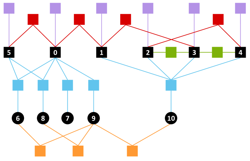
Figure 6: The factor graph representation for our problem. We denote our variables with black nodes, those of which with number $0$–$5$ represent the human parts: torso, RU/LU/RL/LL arm and head, while those with number $6$–$10$ denote the garment attributes: collar, color, neckline, pattern and sleeve. We denote our potentials with colored nodes, with purple ones denoting the unary potential, red denoting the deformation potential, green denoting the consistency potential, orange denoting the attribute co-occurrence potential and cyan denoting the cross potential.

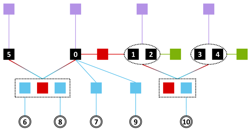
Figure 7: The factor graph representation for inferring human pose. Circle nodes with double boundaries are assigned with fixed values. Symmetric parts are grouped into a super-node, denoted by a dashed oval. For some part nodes, their deformation and cross potential can also be grouped as the associated attribute nodes are now fixed. Note that we don’t draw the garment-specific potentials as they don’t contribute for searching a best pose.

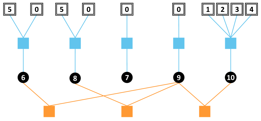
Figure 8: The factor graph representation for inferring attributes. Part nodes are with fixed values and stretching them will not affect the optimal solution. Unary, deformation and consistency potentials of part nodes are not drawn here, as they don’t contribute to searching for a best attribute solution.

II-E2 Inference for Attributes

Referring to Figure 8, we stretch the part variables and remove redundant edges associated with the stretched variables from the original graph as they contribute nothing to this inference step. Note that for the attribute-attribute pairs (i.e. the garment-specific feature), we manually model them as a tree structure. In this way, we can still perform an efficient computation like Algorithm 2.

II-E3 Implementation and Computation Complexity

We write $K=\max_{1\leq i\leq m}K_{i}$ and $T=\max_{1\leq k\leq n}T_{k}$. Now we propose a computation analysis for our Algorithm 2 and give some optimization tricks. In line $3$–$13$, one has to loop over all possible configuration $\mathbf{p}_{\mathbf{i}}$ for the super-node $\mathbf{i}$, and there are at most $2$ nodes in a super-node (see Figure 7); this makes the computation $O(K^{2})$. In fact, note that the computation of unary and strong edge score can be decomposed into a summation of each node (line $4$ and $5$), which indicates that we can separately compute these scores for each node configuration, yielding a computation $O(K)$. Also note that actually we only compute cross score for node $0$ in line $11$ (see Figure 6). Based on this observation, computation on $m(\mathbf{p}_{\mathbf{i}})$ is reduced from $O(K^{2})+O(K^{2})+O(K^{2})+O(K^{2})$ to $O(K)+O(K)+O(K^{2})+O(K)$. In line $14$–$16$, we compute the deformation and cross score for each pair $(\mathbf{p}_{\mathbf{i}},\mathbf{p}_{\mathbf{j}})$, which yields a computation complexity $O(K^{4})$ if without any optimization. For the deformation score, as the decomposition property still holds, the computation is $O(K^{2})$. For the cross score in line $16$, when $k\in\{6,8\}$, the computation is $O(K^{2})$ since we have to loop over all the configurations for nodes ${0}$ and ${5}$. When $k=10$, however, it is not necessary to enumerate the $O(K^{4})$ combinations of node $1$, $2$, $3$ and $4$ if we design a suitable cross-task feature. In our case, $F_{10}(\hat{\mathbf{p}}_{10})$ is the concatenation of the color histogram of each $p_{i}\in\hat{\mathbf{p}}_{10}$, which implicitly owns the decomposition property. Thus, the computation can be reduced to $O(K)$, if we omit the summation operation of these separate scores.

II-F Parameter Sharing

Our work is distinct from other works which address pose estimation and garment attribute in two aspects. First, our carefully designed structured learning model integrates the pose feature and garment attributes into a principle fashion, facilitating a global optimal model. Second, although we derive an iterative inference algorithm to approximate the optima, we allow the parameter sharing between the two steps, i.e. the cross-task features are shared and contribute to both pose estimation and attribute classification (line $5$ and $6$ in Algorithm 1). Therefore, our approach is a paradigm of learning globally and inferring locally, achieving both effectiveness and efficiency (see Section III for experimental justification).

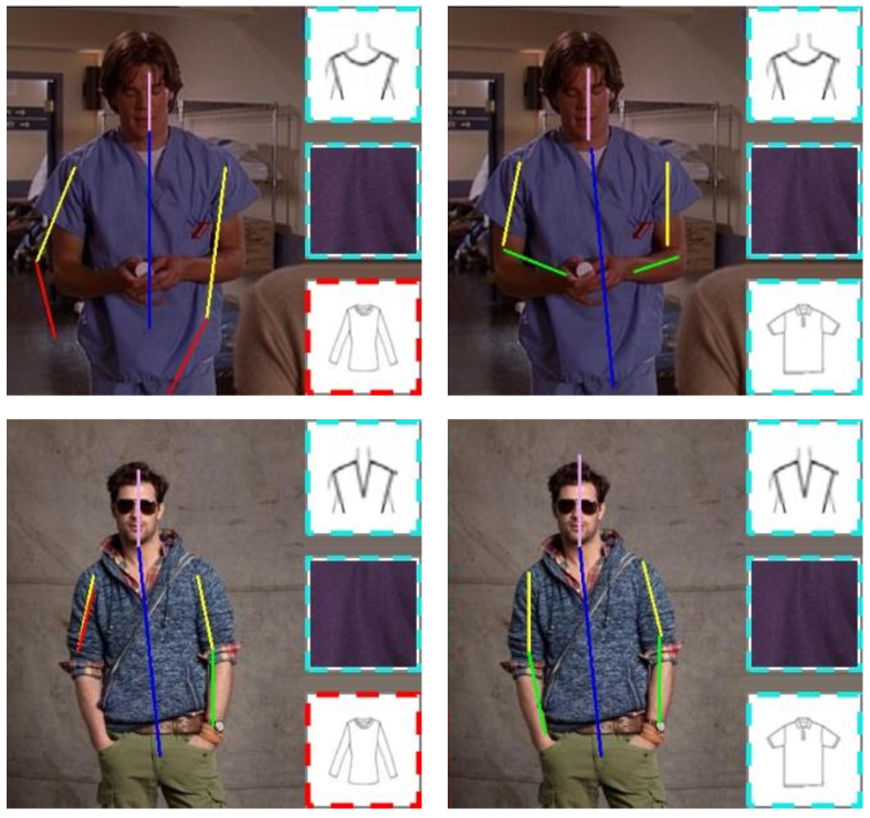
Figure 9: Our joint approach v.s. YDR [3]. Left column: results from [3]. Right column: results from our joint approach. [3] estimates incorrect lower arm(s), which subsequently results in an incorrect prediction for the sleeve attribute. Our joint approach captures the co-relations between the arms and the sleeve attribute and makes a correct estimation for both.

III Experiments

III-A Experimental Settings

In this section, we introduce our experimental settings, including the used datasets, the baselines, the evaluation metrics and the scheme for training structured SVM and inferring for a testing image.

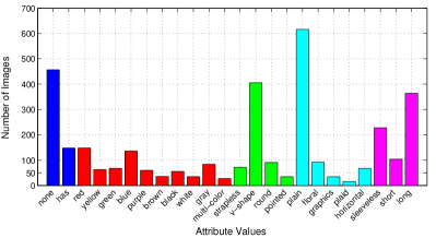
(a) Buffy

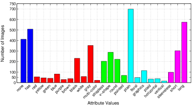
(b) DL

Figure 10: Statistical information for the clothing attribute annotation. Left: Buffy dataset. Right: DL dataset. We use bars with different colors to denote different attributes. Orders from left to right defer to the orders in Figure 3.

Figure 11: Examples lacking some garment attributes. Characters in these images all lack visual cues for specific garment attributes. Persons of the first row wear no garment, thus cannot be labeled with any garment attribute while those of the second row cannot be labeled with part of attributes, e.g., neckline types.

III-A1 Datasets

We conduct experiments on two datasets. The first one is the widely used Buffy dataset [11] consisting of 748 annotated video frames from Buffy TV show. This dataset is proposed as a standard one for HPE task but not originally for GAC task. We manually annotate the garment attributes for the Buffy dataset. The second dataset, called “DL”, contains 1000 daily life photos we collect from websites. Compared with Buffy, the DL dataset possesses more various garment attribute values. In order to obtain quantitative evaluation results, we also manually annotate the human parts and garment attributes for the images in the DL dataset.

Some garment attributes cannot be labeled for the images in which the person does not wear any garment or some attributes’ visual cues cannot be described. In Figure 11, we illustrate some of such samples and list the statistical information for the attributes we annotate in Figure 10.

III-A2 Baselines

We select four state-of-the-art HPE methods as our baselines: Andriluka et al. (ARS) [8], Sapp et al. (STT) [19], Yang and Ramanan (YDR) [3] and Ladicky tl al. (LTZ) [30]. As the code of LTZ is not publicly available, we only evaluate our DL dataset by the first three methods.

Although all these algorithms are primarily designed for HPE, they can actually produce results for GAC: as discussed in [26, 4], the results of HPE can be used for part alignment, which enables the extraction of attribute features. Then for each attribute, we individually train an SVM multi-class model [36]. We use the features described in Table I to train each SVM model. We also compare our GAC results with CGG [4] , which designed a specific pipeline to recognize semantic clothing attributes.

III-A3 Evaluation Metrics

We evaluate the HPE results with the standard metric of Probability of Correct Part (PCP) [9]. The GAC results are evaluated by the Garment Attribute Precision (GAP) criterion, i.e., the classification accuracy for each garment attribute (there are $5$ attributes in this work).

III-A4 Training/Testing

For the Buffy dataset, like [11, 37, 3], we select the images from Episode 3, 4 for training, and Episode 2, 5 and 6 for testing. For our DL dataset, we select randomly 300 images for training and use the remaining 700 images for testing.

As we have discussed in Section III-A1, some images cannot be annotated with some garment attributes. For an image without the garment attribute $c_{j}$, we set all the features related to $c_{j}$ to a zero vector in Eq. (8) when training our structured SVM model and skip evaluation on such attributes. For a person wearing two (or more) garments, we label each garment’s attribute values. Thus the image has several groups of labels in terms of these garments. When training the model, all the groups of labels are used to construct the constraints. When testing a new instance, any attribute value which the algorithm produces is acceptable if the value belongs to any of the groups.

III-B Results

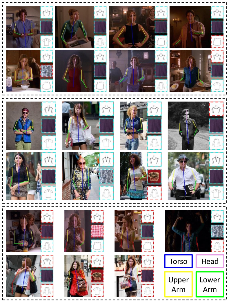
Figure 12: Examples of our results obtained on the Buffy and DL datasets. We demonstrate some good results from Buffy and DL in the first and second panels respectively. Some failure cases are showed in the bottom panel. We use the oriented line to denote the pose estimation. If an HPE result is incorrect, the line is red. We visualize three attributes (neckline, pattern and sleeve) of our GAC results by some icons (see Figure 3 for the icon definition). If a GAC result is incorrect, we use a dashed red rectangle to mark it. Examining the failure cases, we find our algorithm is confused when some human parts are occluded or the human pose is largely variational. Attributes are misclassified when the corresponding parts are mis-detected, or occluded by some objects.

Figure 12 shows some exemplar results produced by our approach. In the following, we shall analyze our approach and compare it with the baselines.

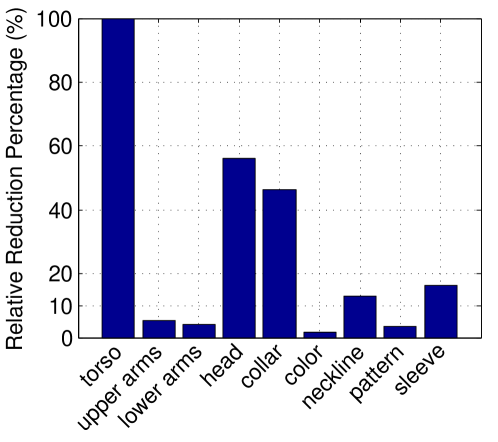
(a) Buffy

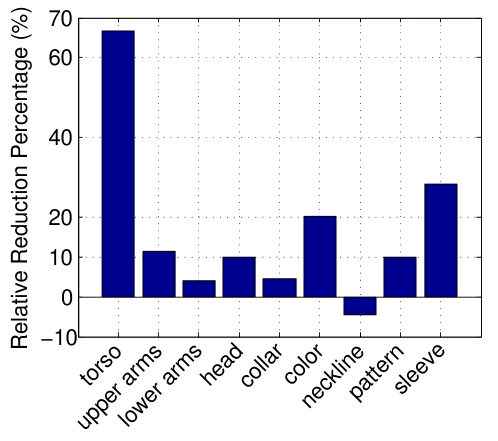
(b) DL

Figure 13: Demonstrating the advantages of combining HPE and GAC together. X-axis: human part and garment attribute. Y-axis: error reduction rate. We compare our joint learning approach with its separated versions on the Buffy and DL dataset, which deal with HPE and GAC individually. The joint approach improves all of the human parts and a majority of garment attributes. This is because there exists a strong correlation between human parts and garment attributes, and our algorithm captures their inter-dependency that improves both simultaneously.

III-B1 Examining the Advantages of Joint Learning

To show the advantages of combining HPE and GAC together, we compare our joint learning approach with its two separated versions: one is an HPE algorithm created by removing the garment-related features in Eq. (8); the other is a GAC algorithm created by ignoring all part-related features. Figure 13 shows the comparison results, which demonstrate the significant advantages of the joint learning over the separated schemes.

Note that the basic appearance constraints of human parts (as [9] considered) have been modeled in the pose-specific features (see Section II-B). Thus, the improvement on HPE is attributed to the integration of garment attribute evidence modeled in Eq. (11), i.e., joint inference. The improvement on GAC can be examined in the same way.

(a) Buffy

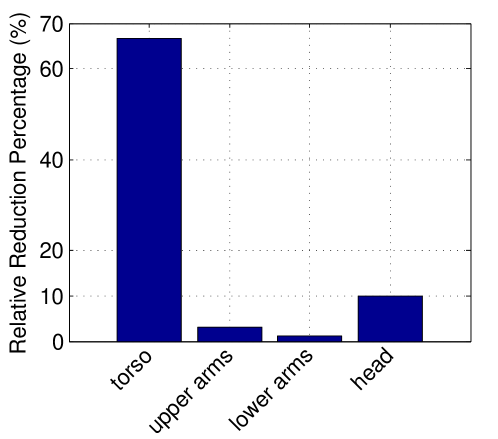
(b) DL

Figure 14: Demonstrating the effectiveness of strong edge evidence. X-axis: human part. Y-axis: error reduction rate. We demonstrate the error reduction rate for employing the strong edge evidence on both Buffy and DL dataset. The strong edge evidence improves the detection rate because it captures the contextual information for a human part, which is complementary to other features.

III-B2 Examining the Effectiveness of Strong Edge

We demonstrate the effectiveness of the strong edge evidence in this section. By setting the $\alpha$ in Eq. (6) with value zero, our inference algorithm 2 produces the results without strong edge evidence. Then we use 3-fold cross validation to tune the parameters $\alpha$ and $\beta$ in Eq. (14). The error reduction rate for employing the strong edge evidence on two datasets is demonstrated in Figure 14. For the Buffy dataset, by using the strong edge evidence, the lower arm accuracy is refined and for the DL dataset, all of the human parts are predicted more precisely.

III-B3 Comparisons with State-of-the-art Algorithms

TABLE II: Comparison with state-of-the-art algorithms on the Buffy dataset.

Method	Torso	U. arms	L. arms	Head	Total
ARS [8]	90.7	79.3	41.2	95.5	73.5
STT [19]	100	95.3	63.0	96.2	85.5
YDR [3]	100	96.6	70.9	99.6	89.1
LTZ [30]	100	97.5	75.4	100	90.9
CGG [4]	–	–	–	–	–
Our Approach	100	96.4	78.4	98.9	91.4

Collar	Color	Neckline	Pattern	Sleeve	Total
70.3	71.7	68.7	80.9	46.6	67.7
77.8	71.2	73.4	80.1	49.2	70.3
82.8	70.8	68.3	80.9	51.5	70.9
–	–	–	–	–	–
89.1	58.4	69.4	80.9	46.2	68.8
88.3	73.1	76.1	81.6	61.7	76.2

TABLE III: Comparison with state-of-the-art algorithms on the DL dataset.

Method	Torso	U. arms	L. arms	Head	Total
ARS [8]	89.4	80.3	60.6	85.0	76.0
STT [19]	99.9	91.1	69.2	97.0	86.2
YDR [3]	99.9	96.0	82.2	99.0	92.5
CGG [4]	–	–	–	–	–
Our Approach	99.9	96.9	83.4	99.1	93.3

Collar	Color	Neckline	Pattern	Sleeve	Total
70.0	55.8	50.9	77.9	60.7	63.1
55.5	58.1	35.9	77.7	61.9	57.8
75.0	58.6	60.0	77.7	64.1	67.1
78.1	69.5	59.2	78.7	68.4	70.8
78.5	67.1	60.0	79.9	68.2	70.7

In this section, we compare our joint approach (with strong edge evidence) with the state-of-the-art algorithm. Note that the results of GAC produced by HPE algorithms have been explained in Section III-A2. Figure 9 gives the exemplar comparison of HPE and GAC results from YDR [3] and our joint approach. On the Buffy dataset, Table II shows that our approach consistently outperforms YDR [3] which is a recently established algorithm and provides the candidates for our approach. We also compare our approach with LTZ [30] which combines pose estimation and segmentation for computation. We improve the lower arms performance and achieve the highest overall accuracy. Table III shows the comparison results on the DL dataset. It can be seen that our approach outperforms all the competing baselines on the task of HPE.

To examine the effectiveness of our approach on GAC, we also compare it with CGG [4], which is a real GAC method. On the Buffy dataset, there is a significant improvement of our approach on the attributes of “color” and “sleeve”, and on the DL dataset, we also reach a competitive performance. The reason of the surprising gain on the Buffy dataset is that human pose of Buffy is more variational than DL. And our model can capture the inter-dependency between human part(s) and garment attributes. However, the pipeline of CGG is step by step, like the work of [23]. Thus it is depressed if the human pose is largely unconstrained.

One may notice that in Table II and Table III, compared with the baselines except CGG [4], the GAC results of our approach are significantly improved when we gain less improvement for HPE on average (see YDR [3] for example). The reasons are twofold. First, the training procedure of our approach is different from that of theirs. Our model is trained in a unified manner, which allows us to integrate more useful features. That is, during the training procedure, our model captures the dependency between human parts and garment attributes (i.e. cross-task features), as well as that between different garment attributes (i.e. garment-specific features). As a result, we finally have a global optimal model for HPE and GAC. However, the competing baselines are trained in a separate manner. That is, given the HPE, each garment attribute is trained individually. Therefore, neither the inter-dependency between human parts and garment attributes, nor that between different garment attributes can be utilized, resulting in a marginal model for multiclass SVM. Second, we search for the optimal prediction for GAC by iteratively updating HPE and GAC, reaching a (local) optimal state of HPE and GAC . However, the baselines can only make a prediction for GAC by the given HPE result.

IV Conclusions and Future Work

Based on the observation that there exist correlations between human parts and garment attributes, we propose to integrate HPE and GAC into a unified procedure and handle both tasks simultaneously. We show that such integration can be seamlessly achieved by using the framework of structured SVM. First, due to the joint feature representation, it is convenient to involve various visual cues such as pose-specific features, garment-specific features and cross-task features. Second, the structured nature of the output space of structured SVM provides us a straightforward way to jointly infer the solutions for several problems (e.g., HPE and GAC). Benefiting from these superiorities, our approach achieves state-of-the-art performance in both HPE and GAC problems, as demonstrated in the experiments. Obviously, the boosted performance can benefit quite many multimedia applications, e.g., online clothing retrieval, clothing recommendation, and we are planning to extend our proposed approach for these applications in our future work.

References

- [1] X. Xiong and F. De la Torre, “Supervised descent method and its applications to face alignment,” in Computer Vision and Pattern Recognition (CVPR), 2013 IEEE Conference on. IEEE, 2013, pp. 532–539.
- [2] M. Andriluka, S. Roth, and B. Schiele, “People-tracking-by-detection and people-detection-by-tracking,” in Computer Vision and Pattern Recognition, 2008. CVPR 2008. IEEE Conference on. IEEE, 2008, pp. 1–8.
- [3] Y. Yang and D. Ramanan, “Articulated pose estimation with flexible mixtures-of-parts,” in Computer Vision and Pattern Recognition (CVPR), 2011 IEEE Conference on. IEEE, 2011, pp. 1385–1392.
- [4] H. Chen, A. Gallagher, and B. Girod, “Describing clothing by semantic attributes,” in Computer Vision–ECCV 2012. Springer, 2012, pp. 609–623.
- [5] P. Arbelaez, M. Maire, C. Fowlkes, and J. Malik, “Contour detection and hierarchical image segmentation,” Pattern Analysis and Machine Intelligence, IEEE Transactions on, vol. 33, no. 5, pp. 898–916, 2011.
- [6] M. A. Fischler and R. A. Elschlager, “The representation and matching of pictorial structures,” IEEE Transactions on Computers, vol. 22, no. 1, pp. 67–92, 1973.
- [7] P. F. Felzenszwalb and D. P. Huttenlocher, “Pictorial structures for object recognition,” International Journal of Computer Vision, vol. 61, no. 1, pp. 55–79, 2005.
- [8] M. Andriluka, S. Roth, and B. Schiele, “Pictorial structures revisited: People detection and articulated pose estimation,” in Computer Vision and Pattern Recognition, 2009. CVPR 2009. IEEE Conference on. IEEE, 2009, pp. 1014–1021.
- [9] M. Eichner and V. Ferrari, “Better appearance models for pictorial structures,” in British Machine Vision Conference, 2009. BMVC 2009., 2009, pp. 1–11.
- [10] P. F. Felzenszwalb, R. B. Girshick, D. McAllester, and D. Ramanan, “Object detection with discriminatively trained part-based models,” Pattern Analysis and Machine Intelligence, IEEE Transactions on, vol. 32, no. 9, pp. 1627–1645, 2010.
- [11] V. Ferrari, M. Marin-Jimenez, and A. Zisserman, “Progressive search space reduction for human pose estimation,” in Computer Vision and Pattern Recognition, 2008. CVPR 2008. IEEE Conference on. IEEE, 2008, pp. 1–8.
- [12] D. Ramanan, “Learning to parse images of articulated bodies,” in NIPS, vol. 1, no. 6, 2006, p. 7.
- [13] B. Rothrock, S. Park, and S.-C. Zhu, “Integrating grammar and segmentation for human pose estimation,” in Computer Vision and Pattern Recognition (CVPR), 2013 IEEE Conference on. IEEE, 2013, pp. 3214–3221.
- [14] J. Wang, Z.-Q. Zhao, X. Hu, Y.-M. Cheung, M. Wang, and X. Wu, “Online group feature selection,” in Proceedings of the Twenty-Third international joint conference on Artificial Intelligence. AAAI Press, 2013, pp. 1757–1763.
- [15] S. Belongie, G. Mori, and J. Malik, “Matching with shape contexts,” in Statistics and Analysis of Shapes. Springer, 2006, pp. 81–105.
- [16] N. Dalal and B. Triggs, “Histograms of oriented gradients for human detection,” in Computer Vision and Pattern Recognition, 2005. CVPR 2005. IEEE Computer Society Conference on, vol. 1. IEEE, 2005, pp. 886–893.
- [17] C. Rother, V. Kolmogorov, and A. Blake, “Grabcut: Interactive foreground extraction using iterated graph cuts,” in ACM Transactions on Graphics (TOG), vol. 23, no. 3. ACM, 2004, pp. 309–314.
- [18] B. Sapp, C. Jordan, and B. Taskar, “Adaptive pose priors for pictorial structures,” in Computer Vision and Pattern Recognition (CVPR), 2010 IEEE Conference on. IEEE, 2010, pp. 422–429.
- [19] B. Sapp, A. Toshev, and B. Taskar, “Cascaded models for articulated pose estimation,” in Computer Vision–ECCV 2010. Springer, 2010, pp. 406–420.
- [20] M. Sun, M. Telaprolu, H. Lee, and S. Savarese, “Efficient and exact map-mrf inference using branch and bound,” in International Conference on Artificial Intelligence and Statistics, 2012, pp. 1134–1142.
- [21] B. Hasan and D. Hogg, “Segmentation using deformable spatial priors with application to clothing.” in BMVC, 2010, pp. 1–11.
- [22] N. Wang and H. Ai, “Who blocks who: Simultaneous clothing segmentation for grouping images,” in Computer Vision (ICCV), 2011 IEEE International Conference on. IEEE, 2011, pp. 1535–1542.
- [23] K. Yamaguchi, M. H. Kiapour, L. E. Ortiz, and T. L. Berg, “Parsing clothing in fashion photographs,” in Computer Vision and Pattern Recognition (CVPR), 2012 IEEE Conference on. IEEE, 2012, pp. 3570–3577.
- [24] S. Liu, J. Feng, Z. Song, T. Zhang, H. Lu, C. Xu, and S. Yan, “Hi, magic closet, tell me what to wear!” in Proceedings of the 20th ACM international conference on Multimedia. ACM, 2012, pp. 619–628.
- [25] X. Wang and T. Zhang, “Clothes search in consumer photos via color matching and attribute learning,” in Proceedings of the 19th ACM international conference on Multimedia. ACM, 2011, pp. 1353–1356.
- [26] S. Liu, Z. Song, G. Liu, C. Xu, H. Lu, and S. Yan, “Street-to-shop: Cross-scenario clothing retrieval via parts alignment and auxiliary set,” in Computer Vision and Pattern Recognition (CVPR), 2012 IEEE Conference on. IEEE, 2012, pp. 3330–3337.
- [27] A. C. Gallagher and T. Chen, “Clothing cosegmentation for recognizing people,” in Computer Vision and Pattern Recognition, 2008. CVPR 2008. IEEE Conference on. IEEE, 2008, pp. 1–8.
- [28] H. Chen, Z. J. Xu, Z. Q. Liu, and S. C. Zhu, “Composite templates for cloth modeling and sketching,” in Computer Vision and Pattern Recognition, 2006 IEEE Computer Society Conference on, vol. 1. IEEE, 2006, pp. 943–950.
- [29] L. Bourdev, S. Maji, and J. Malik, “Describing people: A poselet-based approach to attribute classification,” in Computer Vision (ICCV), 2011 IEEE International Conference on. IEEE, 2011, pp. 1543–1550.
- [30] L. Ladicky, P. H. Torr, and A. Zisserman, “Human pose estimation using a joint pixel-wise and part-wise formulation,” in Computer Vision and Pattern Recognition (CVPR), 2013 IEEE Conference on. IEEE, 2013, pp. 3578–3585.
- [31] I. Tsochantaridis, T. Joachims, T. Hofmann, Y. Altun, and Y. Singer, “Large margin methods for structured and interdependent output variables.” Journal of Machine Learning Research, vol. 6, no. 9, 2005.
- [32] A. Argyriou, T. Evgeniou, and M. Pontil, “Multi-task feature learning,” Advances in neural information processing systems, vol. 19, p. 41, 2007.
- [33] J. Donahue, J. Hoffman, E. Rodner, K. Saenko, and T. Darrell, “Semi-supervised domain adaptation with instance constraints,” in Computer Vision and Pattern Recognition (CVPR), 2013 IEEE Conference on. IEEE, 2013, pp. 668–675.
- [34] T. Ojala, M. Pietikainen, and D. Harwood, “Performance evaluation of texture measures with classification based on kullback discrimination of distributions,” in Pattern Recognition, 1994. Vol. 1-Conference A: Computer Vision & Image Processing., Proceedings of the 12th IAPR International Conference on, vol. 1. IEEE, 1994, pp. 582–585.
- [35] P. F. Felzenszwalb and D. P. Huttenlocher, “Distance transforms of sampled functions.” Theory of computing, vol. 8, no. 1, pp. 415–428, 2012.
- [36] R.-E. Fan, K.-W. Chang, C.-J. Hsieh, X.-R. Wang, and C.-J. Lin, “Liblinear: A library for large linear classification,” The Journal of Machine Learning Research, vol. 9, pp. 1871–1874, 2008.
- [37] V. Ferrari, M. Marin-Jimenez, and A. Zisserman, “Pose search: retrieving people using their pose,” in Computer Vision and Pattern Recognition, 2009. CVPR 2009. IEEE Conference on. IEEE, 2009, pp. 1–8.