Enumerating Maximal Bicliques from a Large Graph using MapReduce

Abstract

We consider the enumeration of maximal bipartite cliques (bicliques) from a large graph, a task central to many practical data mining problems in social network analysis and bioinformatics. We present novel parallel algorithms for the MapReduce platform, and an experimental evaluation using Hadoop MapReduce.

Our algorithm is based on clustering the input graph into smaller sized subgraphs, followed by processing different subgraphs in parallel. Our algorithm uses two ideas that enable it to scale to large graphs: (1) the redundancy in work between different subgraph explorations is minimized through a careful pruning of the search space, and (2) the load on different reducers is balanced through the use of an appropriate total order among the vertices. Our evaluation shows that the algorithm scales to large graphs with millions of edges and tens of millions of maximal bicliques. To our knowledge, this is the first work on maximal biclique enumeration for graphs of this scale.

1 Introduction

A graph is a natural abstraction to model rich relationships in data, and massive graphs are ubiquitous in applications such as online social networks [MMGDB2007, NWS2002], information retrieval from the web [BKMRRSTW2000], citation networks [AJM2004], and physical simulation and modeling [WTCG2012], to name a few. Finding information from such data can often be reduced to a problem of mining features from massive graphs. We consider scalable methods for discovering densely connected subgraphs within a large graph. Mining dense substructures such as cliques, quasi-cliques, bicliques, quasi-bicliques etc. is an important area of study [AACFHS2004, GKT2005, ARS2002, SLGL2006].

A fundamental dense substructure of interest is a biclique. A biclique in a graph $G=(V,E)$ is a pair of subsets of vertices $L\subseteq V$ and $R\subseteq V$ such that (1) $L$ and $R$ are disjoint and (2) there is an edge $(u,v)\in E$ for every $u\in L$ and $v\in R$. For instance, consider the following graph relevant to an online social network, where there are two types of vertices, users and webpages. There is an edge between a user and every webpage that the user “likes” on the social network. A biclique in such a graph consists of a set of users $U$ and a set of webpages $W$ such that every user in $U$ has liked every page in $W$. Such a biclique indicates a set of users who share a common interest, and is valuable for understanding the actions of users on this social network. Often, it is useful to identify only maximal bicliques in a graph, which are those bicliques that are not contained within any other larger bicliques. We consider the problem of enumerating all maximal bicliques from a graph (henceforth referred to as MBE).

Many graph mining tasks have relied on enumerating bicliques to identify significant substructures within the graph. For instance the analysis of web search queries [YM2009] considered the “click-through” graph, where there are two types of vertices, web search queries and web pages. There is an edge from a search query to every page that a user has clicked in response to the search query. MBE was used in clustering queries using the click through graph. MBE has been used in social network analysis, in detection of communities in social networks [LSH2008], and in finding antagonistic communities in trust-distrust networks [LSZL2011]. It has also been applied in detecting communities in the web graph [KRRT1999, RH2005].

In bioinformatics, MBE has been used widely e.g. in construction of the phylogenetic tree of life [DABMMS2004, SDREL2003, YBE2005, NK2008], structure discovery and analysis of protein-protein interaction networks [BZCXZLZSLZLC2003, SLL2011], analysis of gene-phenotype relationships [XPH2012], prediction of miRNA regulatory modules [YM2005], modeling of hot spots at protein interfaces [LL2009], and in analysis of relationships between genotypes, lifestyles, and diseases [MKGR2007]. Other applications include Learning Context Free Grammars [Y2011], finding correlations in databases [J2005], for data compression [AAAAAASS1993], role mining in role based access control [CPOV2010], and process operation scheduling [MGP2011].

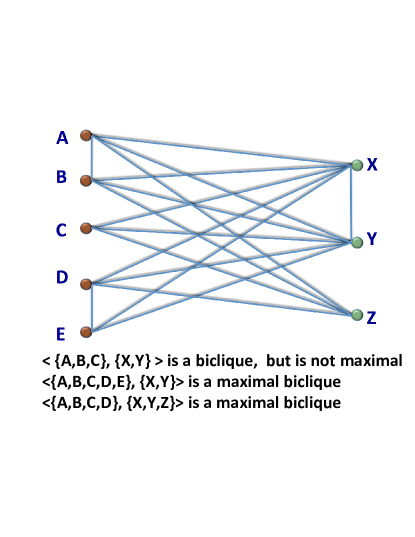
Figure 1: Maximal Bicliques

While it is easy to find a single maximal biclique in a graph, enumerating all maximal bicliques is an NP-hard problem (Peters [P2003]). This does not however mean that typical cases are unsolvable. In fact, there are output-polynomial time algorithms whose theoretical runtime is bounded by a polynomial in the number of vertices in the graph, and the number of maximal bicliques that are output [AACFHS2004]. Thus it is reasonable to expect to be able to devise algorithms for MBE that work on large graphs, as long as the number of maximal bicliques output is not too high.

Current methods for enumerating bicliques have the following drawbacks. Most methods are sequential algorithms that are unable to make use of the power of multiple processors. For handling large graphs, it is imperative to have methods that can process a graph in parallel. Next, they have been evaluated only on small graphs of a few thousands of vertices and a few hundred thousand maximal bicliques, and have not been shown to scale to large graphs. For instance, the popular “consensus” method for biclique enumeration [AACFHS2004] presents experimental data only on graphs of up to 2,000 vertices, and about 140,000 maximal bicliques, and other works [LLSW2005, LSL2006] are also similar. .

Our goal is to design a parallel method that can enumerate maximal bicliques in large graphs, with millions of edges and tens of millions of maximal bicliques, and which can scale with the number of processors.

1.1 Contributions

We present a parallel solution for MBE using the MapReduce framework [DG2008]. At a high level, our approach clusters the input graph into overlapping subgraphs that can be processed independently in parallel, by different reducers. We implement the clustering approach using two different state-of-the-art sequential algorithms for MBE, one based on depth first search [LSL2006], and the other based on the consensus algorithm [AACFHS2004].

For this clustering approach to be effective on large graphs, we needed to augment it with two ideas that significantly improve the parallel performance. The first idea is concerned with reducing the overlap in the work done by different subtasks. It is usually not possible to assign disjoint subgraphs to different processors, and the subgraphs assigned to different tasks will overlap, sometimes significantly. Through a careful partitioning of the search space among the different tasks, we reduce redundant work among the tasks (this partitioning depends on details of the sequential algorithm used at each task).

The second idea is concerned with balancing the load between different tasks. With a graph analysis task such as biclique enumeration, the complexity of different subgraphs varies significantly, depending on the density of edges in the subgraph. Naively done, this can lead to a case where most reducers finish quickly, while only a few take a long time, leading to a poor parallel performance. We present a solution to keep the load more balanced, based on an ordering of vertices, which reduces enumeration load on subgraphs that are dense, and increases the load on subgraphs that are sparse, leading to a better parallel efficiency. We provide some basic statistical analysis of the Reducer runtimes with and without the load balancing to justify our claim.

We give a detailed analysis of the communication costs of the clustering based MapReduce Algorithms described.

We present a direct parallelization of the consensus sequential algorithm [AACFHS2004], using an approach different from clustering. We found that while this approach may use a smaller memory per node that the clustering approach, it requires substantially greater runtime.

Finally, we present detailed experimental results on real-world and synthetic graphs. Overall, the clustering approach (using depth first search), when combined with load balancing and reduction of redundant work, performs the best on large graphs. Our algorithms can process graphs having millions of edges, and tens of millions of maximal bicliques, and can scale out with the cluster size. To our knowledge, these are the largest reported graph instances where bicliques have been successfully enumerated.

We also provide experimental evidence showing that our parallel Algorithm based on depth first search effectively generates only large maximal bicliques. For this we show that the runtime of our parallel algorithm decreases with increase in the size threshold of the generated maximal bicliques.

1.2 Prior and Related Work

Makino et. al [MU2004] describes methods to enumerate all maximal bicliques in a bipartite graph, with the delay between outputting two bicliques bounded by a polynomial in the maximum degree of the graph. Zhang et. al [YEM2008] describe a branch-and-bound algorithm for the same problem. However, these approaches do not work for general graphs, as we consider here.

There is a variant of MBE where we only seek induced maximal bicliques in a graph. An induced maximal biclique is a maximal biclique which is also an induced subgraph; i.e. a maximal biclique $\langle L,R\rangle$ in graph $G$ is an induced maximal biclique if $L$ and $R$ are themselves independent sets in $G$. We consider the non-induced version, where edges are allowed in the graph between two vertices that are both in $L$, or both in $R$ (such edges are of course, not a part of the biclique). The set of maximal bicliques that we output will also contain the set of induced maximal bicliques, which can be obtained by post-processing the output of our algorithm. Note that for a bipartite graph, every maximal biclique is also an induced maximal biclique. Algorithms for Induced MBE include work by Eppstein [E1994], Dias et. al [DFS2005], and Gaspers et. al [GKL2008].

Alexe et. al [AACFHS2004] present an iterative algorithm for non-induced MBE using the “consensus” method, which we briefly review in Section 2.2. Another technique for MBE is based on a recursive depth first search (DFS) [LLSW2005, LSL2006]. [LLSW2005] presents an approach based on a connection with mining closed patterns in a transactional database, and apply the algorithm from [UKA2004], which is based on depth first search. [LSL2006] present a more direct algorithm for biclique enumeration based on depth first search, which we use in our work. This is described in more detail in Section 2.2.

Another approach to MBE is through a reduction to the problem of enumerating maximal cliques, as described by Gély et. al [GNS2009]. Given a graph $G$ on which we need to enumerate maximal bicliques, a new graph $G^{\prime}$ is derived such that through enumerating maximal cliques in $G^{\prime}$ using an algorithm such as [TTT2006, TIAS1977], it is possible to derive the maximal bicliques in $G$. However, this approach is not practical for large graphs since in going from $G$ to $G^{\prime}$, the number of edges in the graph increases significantly.

To our knowledge, the only prior work on parallel algorithms for MBE is by Nataraj and Selvan [NS2009], who use the correspondence between maximal bicliques and closed patterns [LLSW2005] to derive a parallel method for enumerating maximal bicliques. A significant issue is that [NS2009] assumes that the input graph is presented as an adjacency matrix, which is then converted into a transactional database and distributed among the processors. In contrast, we do not assume an adjacency matrix, but assume that the graph is presented as a list of edges. Thus we are able to work on much larger graphs than [NS2009]; the largest graph that they consider has 500 vertices and about 9000 edges.

MBE is related to, but different from the problem of finding the largest sized biclique within a graph (maximum biclique). There are a few variants of the maximum biclique problem, including maximum edge biclique, which seeks the biclique in the graph with the largest number of edges, and maximum vertex biclique, which seeks a biclique with the largest number of edges; for further details and variants, see Dawande et al. [DKST2001]. MBE is harder than finding a maximum biclique, since it enumerates all maximal bicliques, including all maximum bicliques.

2 Preliminaries

We present a formal problem definition, review prior sequential algorithms, and then briefly review the MapReduce parallel programming model that we use.

2.1 Problem Definition

We consider a simple undirected graph $G=(V,E)$ without self-loops or multiple edges, where $V$ is the set of all vertices and $E$ is the set of all edges of the graph. Let $n=\left|{V}\right|$ and $m=\left|{E}\right|$. Graph $H=(V_{1},E_{1})$ is said to be a sub-graph of graph $G=(V,E)$ if $V_{1}\subset V$ and $E_{1}\subset E$. $H$ is known as an induced subgraph if $E_{1}$ consists of all edges of $G$ that connect two vertices in $V_{1}$. For vertex $u\in V$, let $\eta(u)$ denote the vertices adjacent to $u$. For a set of vertices $U\subseteq V$, let $\eta(U)=\bigcup\limits_{u\in U}\eta(u)$. For vertex $u\in V$ and $k>0$, let $\eta^{k}(u)$ denote all vertices that can be reached from $u$ in $k$ hops. For $U\subseteq V$, let $\eta^{k}(U)=\bigcup\limits_{u\in U}\eta^{k}(u)$. We call $\eta^{k}(U)$ as the $k$-neighborhood of $U$. For a set of vertices $U\subseteq V$, let $\Gamma(U)=\bigcap\limits_{u\in U}\eta(u)$.

Definition 1.

A biclique $B=\langle L,R\rangle$ is a subgraph of $G$ containing two non-empty and disjoint vertex sets, $L$ and $R$ such that for any two vertices $u\in L$ and $v\in R$, there is an edge $(u,v)\in E$.

Note that the definition on $B=\langle L,R\rangle$ does not impose any restriction on the existence of edges among the vertices within $R$ or within $L$, i.e., we consider non-induced bicliques.

Definition 2.

A biclique $M=\langle L,R\rangle$ in $G$ is said to be a maximal biclique if there is no other biclique $M^{\prime}=\langle L^{\prime},R^{\prime}\rangle\neq\langle L,R\rangle$ such that $L\subset L^{\prime}$ and $R\subset R^{\prime}$.

The Maximal Biclique Enumeration Problem (MBE) is to enumerate the set of all maximal bicliques in graph $G=(V,E)$.

In our algorithms, we assume that vertex identifiers are unique and are chosen from a totally ordered set. This is usually not a limiting assumption, since vertex identifiers are usually strings which can be ordered using the lexicographic ordering.

2.2 Sequential Algorithms

We describe the two approaches to sequential algorithms for MBE that we consider, one based on a “consensus algorithm” [AACFHS2004], and the other based on depth first search [LSL2006].

Consensus Algorithm

Alexe et. al [AACFHS2004] present an iterative approach to MBE. This type of algorithm starts off with a set of simple “seed” bicliques. In each iteration, it performs a “consensus” operation, which involves performing a cross-product on the set of current candidates bicliques with the seed bicliques, to generate a new set of candidates, and the process continues until the set of candidates does not change anymore. Due to lack of space, we do not present the details here, and refer the reader to [AACFHS2004]. It is proved that these algorithms exactly enumerate the set of maximal bicliques in the input graph.

The consensus approach has a good theoretical guarantee, since its runtime depends on the number of maximal cliques that are output. In particular, the runtime of the MICA version of the algorithm is proved to be bounded by $O\left(n^{3}\cdot N\right)$ where $n$ is the number of vertices and $N$ total number of maximal bicliques in $G$. The consensus algorithm has been found to be adequate for many applications and is quite popular.

We use the consensus algorithm in two ways. One as a candidate method for a sequential algorithm within each cluster. In another, we consider a direct parallelization of the consensus algorithm without using the clustering method.

Sequential DFS Algorithm

The basic sequential depth first approach (DFS) that we use is described in Algorithm 1, based on [LSL2006]. It attempts to expand an existing maximal biclique into a larger one by including additional vertices that qualify, and declares a biclique as maximal if it cannot be expanded any further. The algorithm takes the following inputs: (1) the graph $G=(V,E)$, (2) the current vertex set being processed, $X$, (3) $T$, the tail vertices of $X$, i.e. all vertices that come after $X$ in lexicographical ordering and (4) $s$, the minimum size threshold below which a maximal biclique is not enumerated. $s$ can be set to $1$ so as to enumerate all maximal bicliques in the input graph. However, we can set $s$ to a larger value to enumerate only large maximal bicliques such that for $B=<L,R>$, we have $\left|L\right|\geq s$ and $\left|R\right|\geq s$. The size threshold $s$ is provided as user input. The other inputs are initialized as follows: $X=\varnothing$, $T=V$.

The algorithm recursively searches for maximal bicliques. It increases the size of $X$ by recursively adding vertices from the tail set $T$, and pruning away those vertices from $T$ which along with $X$ do not have any any common vertices in their neighborhood. From the expanded $X$, the algorithm outputs the maximal biclique $\left<\Gamma(\Gamma(X)),\Gamma(X)\right>$.

1

2forall vertex $v\in T$ do

3       if $\left|\Gamma(X\cup\{v\})\right|<s$ then

4             $T\leftarrow T\setminus\{v\}$

5            

6      

7

8if $\left|X\right|+\left|T\right|<s$ then

9       return

10

11Sort vertices in $T$ as per ascending order of $\left|\eta(X\cup\{v\})\right|$

12

13forall vertex $v\in T$ do

14       $T\leftarrow T\setminus\{v\}$

15      

16      if $\left|X\cup\{v\}\right|+\left|T\right|\geq s$ then

17            

18            $N\leftarrow\Gamma(X\cup\{v\})$

19             $Y\leftarrow\Gamma(N)$

20             Biclique $B\leftarrow\left<Y,N\right>$

21            

22            if $(Y\setminus(X\cup\{v\}))\subseteq T$ then

23                   if $\left|Y\right|\geq s$ then

24                         Emit $B$ as a maximal biclique

25                        

26                  

27                  PA($G$, $Y$, $T\setminus Y$, $s$)

28                  

29            

30      

Algorithm 1 Depth First Search: PA($G$,$X$,$T$,$s$)

2.3 MapReduce

MapReduce [DG2008] is a popular framework for processing large data sets on a cluster of commodity hardware. A MapReduce program is written through specifying map and reduce functions. The map function takes as input a key-value pair $\langle k,v\rangle$ and emits zero, one, or more new key-value pairs $\langle k^{\prime},v^{\prime}\rangle$. All tuples with the same value of the key are grouped together and passed to a reduce function, which processes a particular key $k$ and all values that are associated with $k$, and outputs a final list of key-value pairs. The outputs of one MapReduce round can be the input to the next round. Communication happens only when the outputs from the map methods are retrieved by the different reduce methods based on the key, i.e. when data is grouped by keys. Further details are available in [DG2008, GGL2003]. We used Hadoop [W2009, SKRC2010], an open source implementation of MapReduce, on top of a distributed file system HDFS. While we consider the MapReduce framework for this work, our algorithms are generic and can be used with other distributed frameworks like Pregel [MABDHLC2010].

3 MapReduce Algorithms for MBE

In this section, we describe algorithms for MBE using MapReduce. We first present the basic clustering approach, which can be used with any sequential algorithm for MBE, followed by enhancements to the basic clustering approach, and finally the parallel consensus approach.

3.1 Basic Clustering Approach

We first present the basic clustering framework for parallel MBE. The approach is to cluster the input graph into several overlapping sub-graphs (clusters) and then run the sequential DFS algorithm in parallel for each cluster.

For each $v\in V$, the cluster $C(v)$ consists of the induced subgraph on all vertices in $\eta^{2}(v)$ (i.e. the 2-neighborhood of $v$ in $G$). The different clusters $C(v)$ are processed in parallel, and a sequential MBE algorithm is used to enumerate the maximal bicliques from each cluster. While all maximal bicliques in $G$ are indeed output by this approach, the same biclique maybe enumerated multiple times. To suppress duplicates, the following strategy is used: a maximal biclique $B$ arising from cluster $C(v)$ is emitted only if $v$ is the smallest vertex in $B$ according to the total order of the vertices. The basic clustering framework is generic and can be used with any sequential algorithm for MBE. We have considered the clustering algorithm using the DFS and the consensus algorithms for MBE.

Lemma 1.

The basic clustering approach enumerates all maximal bicliques in graph $G=(V,E)$.

Proof.

We show the following two properties. First, every maximal biclique in $G$ must be output as a maximal biclique from cluster $C(v)$ for some $v\in V$. Second, every maximal biclique output from each cluster must be a maximal biclique in $G$. To prove the first direction, consider a maximal biclique $M=\langle L,R\rangle$ in $G$. Let $v$ be the smallest vertex in $M$ in lexicographic order, and without loss of generality suppose that $v\in L$. By the definition of a biclique, for each $u\in R$, $u$ is a neighbor of $v$. Similarly, every vertex $w\in L$ is a neighbor of $v$, and is hence in $\eta^{2}(v)$. Hence $M$ is completely contained in $C(v)$. Note that $M$ is also a maximal biclique in $C(v)$. To see this, note that if $M$ is not maximal biclique in $C(v)$, then $M$ is not maximal in $G$ either.

We prove by contradiction that every maximal biclique in each cluster $C(v)$ is also a maximal biclique in $G$. Consider a biclique $M$ emitted as maximal from cluster $C(v)$ such that it is not maximal in $G$. Then, there exists a maximal biclique $M^{\prime}$ that can be generated by extending $M$. However, it is easy to see that every vertex in $M^{\prime}$ must also be contained in $\eta^{2}(v)$, and hence $M^{\prime}$ is also contained in $C(v)$, contradicting our assumption that $M$ is a maximal biclique in $C(v)$. ∎

There are two problems with the basic clustering approach described above. First is redundant work. Although each maximal biclique in $G$ is emitted only once, it may still be generated multiple times, in different clusters. This redundant work significantly adds to the runtime of the algorithm. Second is an uneven distribution of load among different subproblems. The load on subproblem $C(v)$ depends on two factors, the complexity of cluster $C(v)$ (i.e. the number and size of maximal bicliques within $C(v)$) and the position of $v$ in the total order of the vertices. The earlier $v$ appears in the total order, the greater is the likelihood that a maximum biclique in $C(v)$ has $v$ has its smallest vertex, and hence the greater is the responsibility for emitting bicliques that are maximal within $C(v)$. Using a lexicographic ordering of the vertices may lead to a significantly increased workload for clusters of lower numbered vertices and a correspondingly low workload for clusters of higher numbered vertices.

Table 1: Different versions of Parallel Algorithms based on Depth First Search (DFS)

Label	Algorithm
CDFS	Clustering based on Depth First Search (DFS)
CD0	CDFS + Reducing Redundant Work, without Load Balancing
CD1	CDFS + Reducing Redundant Work + Load Balancing using Degree
CD2	CDFS + Reducing Redundant Work + Load Balancing using Size of 2-neighborhood

3.2 Reducing Redundant Work

In order to reduce redundant work done at different clusters, we modify the sequential DFS algorithm for MBE that is executed at each reducer. We first observe that in cluster $C(v)$, the only maximal bicliques that matter are those with $v$ as the smallest vertex; the remaining maximal bicliques in $C(v)$ will not be emitted by this reducer, and need not be searched for here. We use this to prune the search space of the sequential DFS algorithm used at the reducer.

All search paths in the algorithm which lead to a maximal biclique having a vertex less than $v$ can be pruned away. Hence, before starting the DFS, we prune away all vertices in the Tail set that are less than $v$, as described in Algorithm 6. Also, in DFS Algorithm 7, we prune the search path in Line 12 if the generated neighborhood contains a vertex less than $v$ – maximal bicliques along this search path will not have $v$ as the smallest vertex. Finally in Line 19 of Algorithm 7, we emit a maximal biclique only if the smallest vertex is the same as the key of the reducer in Algorithm 6.

The above algorithm, the “optimized DFS clustering algorithm”, or “CD0” for short, is described in Algorithm 2. This takes two rounds of MapReduce. The first round, described in Algorithms 3 (map) and 4 (reduce), is responsible for generating the 1-neighborhood for each vertex. The second round, described in Algorithms 5 (map) and 6 (reduce) first constructs the clusters $C(v)$ and runs the optimized sequential pruning algorithm at the reducer. Note that Algorithm 6 passes the size threshold $s$ while calling the optimized DFS Algorithm 7. The size threshold is an user input and can be passed on to Reducer (Algorithm 6) by using the Configuration parameters of Hadoop. Like the sequential algorithm, this parameter can be set to $1$ to enumerate all maximal bicliques and to a larger value to enumerate only large maximal bicliques.

Input: Edge List of $G=(V,E)$

1 Generate Adjacency List (Map) – Algorithm 3

2 Generate Adjacency List (Reduce) – Algorithm 4

3 Create Two Neighborhood (Map) – Algorithm 5

4 Create Two Neighborhood (Reduce) – DFS – Algorithm 6

Algorithm 2 Algorithm CD0

Input: Edge $(x,y)$

1 Emit ($key\leftarrow x$,$value\leftarrow y$)

2 Emit ($key\leftarrow y$,$value\leftarrow x$)

Algorithm 3 Generate Adjacency List – Map

Input: $key\leftarrow v$,$value\leftarrow${Neighbors of $v$}

1 $neighborhood\leftarrow\varnothing$

2 forall $val\in value$ do

3       $neighborhood\leftarrow neighborhood\cup val$

4      

5$N\leftarrow\langle v,neighborhood\rangle$

6 Emit ($key\leftarrow\varnothing$,$value\leftarrow N$)

Algorithm 4 Generate Adjacency List – Reduce

Input: $N\leftarrow\langle v,neighborhood\rangle$

1 Emit ($key\leftarrow v$,$value\leftarrow N$)

2 forall $y\in neighborhood$ do

3       Emit ($key\leftarrow y$,$value\leftarrow N$)

4      

Algorithm 5 Create Two Neighborhood – Map

Input: $key\leftarrow v$, $value\leftarrow$ {2–neighborhood of $v$}

1 $G^{\prime}=(V^{\prime},E^{\prime})\leftarrow$ Induced subgraph on $\eta^{2}(v)$

2 $X\leftarrow\varnothing$

3 $T\leftarrow V^{\prime}$

4 forall vertex $t\in T$ do

5       if $t<key$ then

6             $T\leftarrow T\setminus\{t\}$

7            

8      

9CD0_Seq($G^{\prime}$, $X$, $T$, $key$, $s$)

Algorithm 6 Create Two Neighborhood (DFS) – Reduce

Input: $G^{\prime}$,$X$,$T$,$key$,$s$

1

2forall vertex $v\in T$ do

3       if $\left|\Gamma(X\cup\{v\})\right|<s$ then

4             $T\leftarrow T\setminus\{v\}$

5            

6      

7

8if $\left|X\right|+\left|T\right|<s$ then

9       return

10

11Sort vertices in $T$ as per ascending order of $\left|\Gamma(X\cup\{v\})\right|$

12

13forall vertex $v\in T$ do

14       $T\leftarrow T\setminus\{v\}$

15      

16      if $\left|X\cup\{v\}\right|+\left|T\right|\geq s$ then

17            

18            $N\leftarrow\Gamma(X\cup\{v\})$

19             $Y\leftarrow\Gamma(N)$

20            

21            if  $Y$ contains vertices smaller than $key$ then

22                   continue

23                  

24            

25            Biclique $B\leftarrow\left<Y,N\right>$

26            

27            if $(Y\setminus(X\cup\{v\}))\subseteq T$ then

28                   if $\left|Y\right|\geq s$ then

29                         $v_{s}\leftarrow$ Smallest vertex in $B$

30                         if $v_{s}=key$ then

31                               // Maximal biclique found

32                               Emit ($key\leftarrow\varnothing$,$value\leftarrow B$)

33                              

34                        

35                  

36                  CD0_Seq($G^{\prime}$, $Y$, $T\setminus Y$, $key$, $s$)

37                  

38            

39      

40

Algorithm 7 Optimized DFS – CD0_Seq

Lemma 2.

No maximal biclique in G is emitted by more than one reducer in Algorithm 7.

Proof.

Without the loss in generality, consider any maximal biclique $M~{}=~{}<L,R>$. Let $a\in\{L\cup R\}$ be the smallest vertex in $\{L\cup R\}$. Consider the reducer with $key=a$. In Line 20 of Algorithm 7, a maximal biclique is emitted only if the condition in line 18 is satisfied. This condition is satisfied by the reducer with $key=a$. However, this condition is not satisfied for any reducer such that $key\neq a$. Thus maximal biclique $M$ is emitted only for the reducer with $key=a$. ∎

Lemma 3.

Algorithm 2 generates all maximal bicliques in a graph.

Proof.

The correctness of this Lemma can be proved from Lemmas 1 and 2. Algorithm  2 generates the 2-neighborhood induced sub–graph of each vertex in $G$. It then runs the Sequential DFS algorithm with the optimizations explained above.

The correctness relies on the following two observations: Firstly, from Lemma 2, a maximal biclique is emitted from a reducer only if the smallest vertex in the biclique is same as the reducer key. Secondly, no vertex is ever removed from the set $X$. The set $X$ thus always grows in size and never gets smaller in the course of the depth-first search. This is because the set $Y$ is generated from set $X$ in line 11 of Algorithm 7 and the set $Y$ is passed as the new set $X$ for the next level of recursion. The set $Y$ is generated from the set $X$ by taking the neighborhood of neighborhood of set $X$. $\eta(X)$ contains the set of all vertices connected to all vertices in $X$. Then $\Gamma(\Gamma(X))$ contains all vertices connected to all vertices in $\eta(X)$. This must include $X$. Hence $Y\supseteq X$.

From the above two observations we can prove the Lemma. Since we emit only those maximal bicliques for which the smallest vertices is the same as the reducer key $k$, we do not need to search the paths that produce maximal bicliques with smallest vertex less than $k$. Also, since no vertex is ever removed from the set $X$ through the recursion path, we can be sure that at no point in the execution of the algorithm we will have $v\in X$ such that $v<k$. Now the set $T$ can be considered as the candidate set as we always add elements to set $X$ from set $T$. Thus in Algorithm 6 we remove all vertices from the set $T$ that are less than $k$. Further in Algorithm 7, if we generate a maximal biclique in Line 12 with minimum vertex less than $k$ then we prune the search tree through that path as all further maximal bicliques found in that search path will contain that vertex less than $k$. ∎

3.3 Load Balancing

Input: Edge List of $G=(V,E)$

1 Generate Adjacency List (Map) – Algorithm 3

2 Generate Adjacency List (Reduce) – Algorithm 4

3 Send vertex property (Map) – Algorithm 5

4 Send vertex property (Reduce) – Algorithm 9

5 Create Two Neighborhood (Map) – Algorithm 10

6 Create Two Neighborhood (Reduce) – Algorithm 11

Algorithm 8 Algorithms CD1 and CD2

Input: $key\leftarrow v$, $value\leftarrow$ {2–neighborhoods of $v$}

1 $S\leftarrow$ 2–neighbors of $v$

2 $neighborhood\leftarrow$ Compute neighborhood of $v$ from $S$

3 $N\leftarrow\langle v,neighborhood\rangle$

4 // Need to pass neighborhood for Round 3

5 Emit ($key\leftarrow\varnothing$,$value\leftarrow N$)

6 // Need to send vertex property to all 2--neighbors

7 $p\leftarrow$ Value of vertex property of $v$ from $S$

8 forall vertices $s\in S$ do

9       Emit($key\leftarrow\varnothing$,$value\leftarrow[s,v,p]$)

10      

Algorithm 9 Send vertex property – Reduce

Input: $N\leftarrow\langle v,neighborhood\rangle$ OR $[s,v,p]$

1 if $Input=N$ then

2       Emit ($key\leftarrow v$,$value\leftarrow N$)

3       forall $y\in neighborhood$ do

4             Emit ($key\leftarrow y$,$value\leftarrow N$)

5            

6      

7else if $Value=[s,v,p]$ then

8       Emit ($key\leftarrow s$,$value\leftarrow[v,p]$)

9      

Algorithm 10 Create Two Neighborhood with vertex property – Map

Input: $key\leftarrow v$, $value\leftarrow$ {$\eta^{2}(v)$ along with vertex properties}

1 $G^{\prime}=(V^{\prime},E^{\prime})\leftarrow$ Induced subgraph on $\eta^{2}(v)$

2 $Map\leftarrow$ HashMap of vertex and vertex property created from $value$ required to compute the new ordering

3 $X\leftarrow\varnothing$

4 $T\leftarrow V^{\prime}$

5 forall vertex $t\in T$ do

6       if $t<key$ in the new ordering then

7             $T\leftarrow T\setminus\{t\}$

8            

9      

10CDL_Seq($G^{\prime}$, $X$, $T$, $key$,$Map$, $s$)

Algorithm 11 Create Two Neighborhood with vertex property (DFS) – Reduce

Input: $G^{\prime}$,$X$,$T$,$key$,$Map$,$s$

1

2forall vertex $v\in T$ do

3       if $\left|\Gamma(X\cup\{v\})\right|<s$ then

4             $T\leftarrow T\setminus\{v\}$

5            

6      

7

8if $\left|X\right|+\left|T\right|<s$ then

9       return

10

11Sort vertices in $T$ as per ascending order of $\left|\Gamma(X\cup\{v\})\right|$

12

13forall vertex $v\in T$ do

14       $T\leftarrow T\setminus\{v\}$

15      

16      if $\left|X\cup\{v\}\right|+\left|T\right|\geq s$ then

17            

18            $N\leftarrow\Gamma(X\cup\{v\})$

19             $Y\leftarrow\Gamma(N)$

20            

21            if  $Y$ contains vertices smaller than $key$ in the new ordering then

22                   continue

23                  

24            

25            Biclique $B\leftarrow\left<Y,N\right>$

26            

27            if $(Y\setminus(X\cup\{v\}))\subseteq T$ then

28                   if $\left|Y\right|\geq s$ then

29                         $v_{s}\leftarrow$ Smallest vertex in $B$ in the new ordering

30                         if $v_{s}=key$ then

31                               // Maximal biclique found

32                               Emit ($key\leftarrow\varnothing$,$value\leftarrow B$)

33                              

34                        

35                  

36                  CDL_Seq($G^{\prime}$, $Y$, $T\setminus Y$, $key$,$Map$, $s$)

37                  

38            

39      

40

Algorithm 12 Load Balanced DFS – CDL_Seq

In Algorithm 2, lexicographical ordering was used to order the vertices, which is agnostic of the properties of the cluster $C(v)$. The way the optimized DFS works (Algorithm 7), a reducer processing a vertex that is earlier in the total order is responsible for emitting more of the maximal bicliques within its cluster.

For improving load balance, we adjust the position of vertex $v$ in the total order according to the properties of its cluster $C(v)$. Intuitively, the more complex cluster $C(v)$ is (i.e. more and larger the maximal bicliques), the higher should be position of $v$ in the total order, so that the burden on the reducer handling $C(v)$ is reduced. While it is hard to compute (or estimate) the number of maximal bicliques in $C(v)$, we consider two properties of vertex $v$ that are simpler to estimate, to determine the relative ordering of $v$ in the total order: (1) Size of 1-neighborhood of $v$ (Degree), and (2) Size of 2-neighborhood of $v$

In case of a tie, the vertex ID is used as a tiebreaker. These approaches were considered since vertices with higher degree are potentially part of a denser part of the graph and are contained within a greater number of maximal bicliques. The size of the 2-neighborhood gives the number of vertices in $C(v)$ and may provide a better estimate of the complexity of handling $C(v)$, but this is more expensive to compute than the size of the 1-neighborhood of the vertex.

The discussion below is generic and holds for both approaches to load balancing. To run the load balanced version of DFS, the reducer running the sequential algorithm must now have the following information for the vertex (key of the reducer) : (1) 2-neighborhood induced subgraph, and (2) vertex property for every vertex in the 2-neighborhood induced subgraph, where “vertex property” is the property used to determine the total order, be it the degree of the vertex or the size of the 2-neighborhood. The second piece of information is required to compute the new vertex ordering. However, the reducer of the second round does not have this information for every vertex in $C(v)$, and a third round of MapReduce is needed to disseminate this information among all reducers. Further details are described in Algorithm 8. The DFS sequential algorithm for load balancing, described in Algorithm 11, is the same as the optimized DFS sequential algorithm 6, except that it orders using the vertex property (ties broken by IDs) rather than the simple lexicographic ordering.

3.4 Communication Complexity

We consider the communication complexity of Algorithms CD0, CD1 and CD2. For input graph $G=\left(V,E\right)$, we know that $n=\left|V\right|$ and $m=\left|E\right|$. Let us assume $\Delta$ to be the largest degree and $\bar{d}$ to be the average degree of vertices, where $\bar{d}=m/n$. Also, let $\beta$ be the Output Size.

Definition 3.

Communication complexity of a MapReduce Algorithm $\mathcal{A}$ for Round $r$ is denoted by $\mathcal{C}^{r}_{\mathcal{A}}$ and is defined as the sum of the total number of bytes emitted by all Mappers and the total number of bytes emitted by all the Reducers. We consider the output size for Reducers contributing to $\mathcal{C}^{r}_{\mathcal{A}}$ as each Reducer writes into the distributed file system incurring communication.

Definition 4.

Let $\mathcal{C}_{\mathcal{A}}$ denote the total communication complexity for a MapReduce Algorithm $\mathcal{A}$ having $R$ rounds. We define $\mathcal{C}_{\mathcal{A}}$ $=$ $\sum\limits_{r=1}^{R}\mathcal{C}^{r}_{\mathcal{A}}$.

Lemma 4.

Total communication complexity of Algorithm CD0 is $O\left(m\cdot\Delta+\beta\right)$.

Proof.

Algorithm CD0 has two rounds of MapReduce. For the first round, Algorithm 3, which is the Map method emits each edge twice, resulting in a communication complexity of $O\left(m\right)$. Similarly, Algorithm 4, which is the reducer emits each adjacency list once. This also results in a communication complexity of $O\left(m\right)$. Hence total communication complexity of the first round is $O\left(m\right)$.

Now let us consider the second round of MapReduce. The total communication between the Map and Reduce methods (Algorithms 5 and 6 respectively) can be computed by analyzing how much data is received by all Reducers. Each reducer receives the adjacency list of all the neighbors of the key. Let $d_{i}$ be the degree of vertex $v_{i}$, for $v_{i}\in V$, $i=1,..,n$. Total communication is thus $\sum\limits_{i=1}^{n}{d_{i}}^{2}$ $={d_{1}}^{2}+{d_{2}}^{2}+\cdot\cdot\cdot{d_{n}}^{2}$. This is $O\left(\left(d_{1}+d_{2}+\cdot\cdot\cdot+d_{n}\right)\cdot\Delta\right)$ $=O\left(n\cdot\bar{d}\cdot\Delta\right)$. Since $\bar{d}=m/n$, total communication becomes $O\left(m\cdot\Delta\right)$. The output from the final Reducer (Algorithm 6) is the collection of all maximal bicliques and hence the resulting communication cost is $O\left(\beta\right)$. Combining two rounds, total communication complexity becomes $O\left(m+m\cdot\Delta+\beta\right)$. $=O\left(m\cdot\Delta+\beta\right)$. ∎

Lemma 5.

Total communication complexity of Algorithm CD1 / CD2 is $O\left(m\cdot\Delta+\beta\right)$.

Proof.

First, note that both Algorithms CD1 and CD2 have the same communication complexity and observe that the first round uses the same Map and Reduce methods as CD0. Thus communication for Round 1 is $O\left(m\right)$. Again, note that Map method for Round 2 is same as CD0 and hence by Lemma 4, communication for Round 2 is $O\left(m\cdot\Delta\right)$.

The Reducer (Algorithm 9) of Round 2 sends the vertex property information to all its 2–neighbors. Thus every reducer receives information about all of its 2–neighbors. This makes the total output size of Reducer to be $O\left(m\cdot\Delta\right)$. The Map method of Round 3 (Algorithm 10) sends out the 2–neighborhood information as well as the vertex information to all vertices in 2–neighborhood. Thus communication cost becomes $O\left(m\cdot\Delta\right)$. The Reducer (Algorithm 11) emits all maximal bicliques and hence the resulting communication cost is $O\left(\beta\right)$. Thus total communication cost for Algorithms CD1 and CD2 is is $O\left(m\cdot\Delta+\beta\right)$. ∎

3.5 Parallel Consensus

We briefly describe another approach which directly parallelizes the consensus sequential algorithm of [AACFHS2004], in a manner different from the clustering approach. The motivation for this approach is as follows. The clustering approach has the following potential drawback, it requires each cluster $C(v)$ to have the entire 2-neighborhood of $v$. For dense graphs, the size of the 2-neighborhood of a vertex can be large, so that the complexity of each reduce task can be substantial. With the nature of the MapReduce model, dynamic load balancing among the reducers is not (easily) possible, so that load balancing will always be an issue for non-uniform, irregular computations.

Unlike the parallel DFS algorithm which works on subgraphs of $G$, the consensus algorithm is always directly dealing with bicliques within graph $G$. At a high level, it performs two operations repeatedly (1) a “consensus” operation, which creates new bicliques by considering the combination of existing bicliques, and (2) an “extension” operation, which extends existing bicliques to form new maximal bicliques. There is also a need for eliminating duplicates after each iteration, and also a step needed for detecting convergence, which happens when the set of maximal bicliques is stable and does not change further.

We developed a parallel version of each of these operations, by performing the consensus, extension, duplicate removal, and convergence test using MapReduce. We omit the details due to lack of space, but present experimental results from our implementations.

4 Experimental Results

Table 2: Various properties of the input graphs used, and runtime of different algorithms using 100 reducers. DNF means that the algorithm did not finish in 12 hours. The size threshold was set as $1$ to enumerate all maximal bicliques. Runtime includes overhead of all MapReduce rounds including graph clustering, i.e. formation of 2–neighborhood.

Label	Input Graph	#vertices	#edges	#max–bicliques	Output Size	CDFS	CD0	CD1	CD2
1	p2p-Gnutella09	8114	26013	20332	407558	113	92	132	130
2	email-EuAll-0.6	125551	168087	292008	9161154	42023	4640	683	626
3	com-Amazon	334863	925872	706854	12739908	186	113	185	221
4	amazon0302	262111	1234877	886776	14553776	396	272	151	153
5	com-DBLP-0.6	251226	419573	1875185	82814962	1659	409	374	478
6	email-EuAll-0.4	175944	252075	2003426	111370926	DNF	DNF	6365	4154
7	ego-Facebook-0.6	3928	35397	6597716	315555360	8657	3858	1512	2943
8	loc-BrightKite-0.6	49142	171421	10075745	777419528	28585	11451	2506	2998
9	web-NotreDame-0.8	150615	300398	19941634	942300172	DNF	DNF	1688	2327
10	ca-GrQc-0.4	5021	17409	16133368	3101214314	37279	6895	5790	6374
11	ER-50K	50000	275659	51756	1116752	96	89	133	136
12	ER-60K	60000	330015	61821	1334716	98	89	135	135
13	ER-70K	70000	393410	71962	1589408	98	90	135	132
14	ER-80K	80000	448289	81983	1809070	102	90	136	134
15	ER-90K	90000	526943	92214	2125544	109	96	142	140
16	ER-100K	100000	600038	102663	2421528	114	97	144	143
17	ER-250K	250000	1562707	252996	6274864	167	114	165	162
18	ER-500K	500000	3751823	506319	15057870	374	167	251	252
19	Bipartite-50K-100K	150000	1999002	306874	9256056	873	183	227	253

$\begin{array}{c}\end{array}$

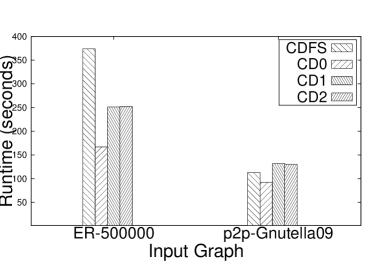
(a) ER-500Kandp2p-Gnutella09

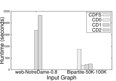
(b) web-NotreDame-