Fractional Maps and Fractional Attractors. Part II: Fractional Difference Caputo $\alpha$-Families of Maps

Edelman M Department of Physics, Stern College at Yeshiva University, 245 Lexington Ave, New York, NY 10016, USA, (e-mail: medelma1@yu.edu). Courant Institute of Mathematical Sciences, New York University, 251 Mercer St., New York, NY 10012, USA, (e-mail:edelman@cims.nyu.edu).
Abstract

In this paper we extend the notion of an $\alpha$-family of maps to discrete systems defined by simple difference equations with the fractional Caputo difference operator. The equations considered are equivalent to maps with falling factorial-law memory which is asymptotically power-law memory. We introduce the fractional difference Universal, Standard, and Logistic $\alpha$-Families of Maps and propose to use them to study general properties of discrete nonlinear systems with asymptotically power-law memory.

keywords:
fractinal derivative \sepfractional difference \sepattractor \sepdiscrete map \seppower-law \sepmemory
โ€ โ€ thanks: The author acknowledges support from the Joseph Alexander Foundation, Yeshiva University.

1 Introduction

Systems with memory are common in biology, social sciences, physics, and engineering (see review Edelman (2014c)). The most frequently encountered type of memory in natural and engineering systems is power-law memory. This leads to the possibility of describing them by fractional differential equations, which have power-law kernels. Nonlinear integro-differential fractional equations are difficult to simulate numerically - this is why in Tarasov and Zaslavsky (2008) the authors introduced fractional maps, which are equivalent to fractional differential equations of nonlinear systems experiencing periodic delta function-kicks, and proposed to use them for the investigation of general properties of nonlinear fractional dynamical systems. Bifurcation diagrams in the fractional Logistic Map related to a scheme of numerical integration of fractional differential equations were considered by Stanislavsky (2006).

An adequate description of discrete natural systems with memory can be obtained by using fractional difference equations (see Miller and Ross (1989); Gray and Zhang (1988); Agarwal (2000); Atici and Eloe (2009); Anastassiou (2009); Chen etย al. (2011); Wu etย al. (2014); Wu and Baleanu (2014)). In Chen etย al. (2011); Wu etย al. (2014); Wu and Baleanu (2014) the authors demonstrated that in some cases fractional difference equations are equivalent to maps (which we will call fractional difference maps) with falling factorial-law memory, where falling factorial function is defined as

$$t^{(\alpha)}=\frac{\Gamma(t+1)}{\Gamma(t+1-\alpha)}.$$ (1)

Falling factorial-law memory is asymptotically power-law memory -

$$\lim_{t\rightarrow\infty}\frac{\Gamma(t+1)}{\Gamma(t+1-\alpha)t^{\alpha}}=1,\ \ \ \alpha\in\mathbb{R},$$ (2)

and we may expect that fractional difference maps have properties similar to the properties of fractional maps.

The goal of the present paper is to introduce fractional difference families of maps depending on memory and nonlinearity parameters consistent with the previous research of fractional maps (see Edelman (2014c); Tarasov and Zaslavsky (2008); Edelman and Tarasov (2009); Tarasov (2009a, b, 2011); Edelman (2011); Edelman and Taieb (2013); Edelman (2013a, b)) in order to prepare a background for an investigation of general properties of systems with asymptotically power-law memory.

In the next section (Sec.ย 2) we will remind the reader how the regular Universal, Standard, and Logistic Maps (see Chirikov (1979.); Lichtenberg and Lieberman (1992); Zaslavsky (2008); May (1976)) are generalized to obtain fractional Caputo $\alpha$-Families of Maps ($\alpha$FM). In Sec.ย 3 weโ€™ll present some basics on fractional difference/sum operators, which will be used in Sec.ย 4 to derive the fractional difference Caputo Universal, Standard, and Logistic $\alpha$FMs. In Sec.ย 5 weโ€™ll present some results on properties of fractional difference Caputo Standard $\alpha$FM.

2 Fractional $\alpha$-Families of Maps

Fractional $\alpha$FM were introduced in Edelman (2013a), further investigated in Edelman (2013b), and reviewed in Edelman (2014c). The Universal $\alpha$FM was obtained by integrating the following equation:

$$\frac{d^{\alpha}x}{dt^{\alpha}}+G_{K}(x(t-\Delta))\sum^{\infty}_{k=-\infty}\delta\Bigl{(}t-(k+\varepsilon)\Bigr{)}=0,$$ (3)

where $\varepsilon>\Delta>0$, $\alpha\in\mathbb{R}$, $\alpha>0$, $\varepsilon\rightarrow 0$, with the initial conditions corresponding to the type of fractional derivative to be used. $G_{K}(x)$ is a nonlinear function which depends on the nonlinearity parameter $K$. It is called Universal because integration of Eq.ย (3) in the case $\alpha=2$ and $G_{K}(x)=KG(x)$ produces the regular Universal Map (see Zaslavsky (2008)). In what follows the author considers Eq.ย (3) with the left-sided Caputo fractional derivative (see Samko etย al. (1993); Kilbas etย al. (2006); Podlubny (1999))

${}_{0}^{C}D^{\alpha}_{t}x(t)=_{0}I^{N-\alpha}_{t}\ D^{N}_{t}x(t)$
$\displaystyle=\frac{1}{\Gamma(N-\alpha)}\int^{t}_{0}\frac{D^{N}_{\tau}x(\tau)d\tau}{(t-\tau)^{\alpha-N+1}},\quad(N=\lceil\alpha\rceil),$ (4)

where $N\in\mathbb{Z}$, $D^{N}_{t}=d^{N}/dt^{N}$, ${}_{0}I^{\alpha}_{t}$ is a fractional integral, $\Gamma()$ is the gamma function, and the initial conditions are

$$(D^{k}_{t}x)(0+)=b_{k},\ \ \ k=0,...,N-1.$$ (5)

There are two reasons to restrict the consideration in this paper to the Caputo case (the Riemann-Liouville case wonโ€™t be considered): a) as in the case of fractional differential equations, in the case of fractional difference equations it is much easier to define initial conditions for Caputo difference equations than for Riemann-Liouville difference equations; b) the main goal of this work is to compare fractional and fractional difference maps, and the case of Caputo maps serves the purpose. Comparison of the Riemann-Liouville and Caputo Standard Maps was considered in Edelman (2011).

The problem Eqs.ย (3)โ€“(5) is equivalent to the Volterra integral equation of the second kind ($t>0$) Kilbas etย al. (2006)

$\displaystyle x(t)=\sum^{N-1}_{k=0}\frac{b_{k}}{k!}t^{k}$
$\displaystyle-\frac{1}{\Gamma(\alpha)}\int^{t}_{0}d\tau\frac{G_{K}(x(\tau-\Delta))}{(t-\tau)^{1-\alpha}}\sum^{\infty}_{k=-\infty}\delta\Bigl{(}\tau-(k+\varepsilon)\Bigr{)}.$ (6)

After the introduction x(s)โ€‹(t)=Dtsโ€‹xโ€‹(t)superscript๐‘ฅ๐‘ ๐‘กsubscriptsuperscript๐ท๐‘ ๐‘ก๐‘ฅ๐‘กx^{(s)}(t)=D^{s}_{t}x(t) the Caputo Universal $\alpha$FM can be written as (see Tarasov (2011))

xn+1(s)=โˆ‘k=0Nโˆ’sโˆ’1x0(k+s)k!โ€‹(n+1)ksubscriptsuperscript๐‘ฅ๐‘ ๐‘›1subscriptsuperscript๐‘๐‘ 1๐‘˜0subscriptsuperscript๐‘ฅ๐‘˜๐‘ 0๐‘˜superscript๐‘›1๐‘˜\displaystyle x^{(s)}_{n+1}=\sum^{N-s-1}_{k=0}\frac{x^{(k+s)}_{0}}{k!}(n+1)^{k}
โˆ’1ฮ“โ€‹(ฮฑโˆ’s)โ€‹โˆ‘k=0nGKโ€‹(xk)โ€‹(nโˆ’k+1)ฮฑโˆ’sโˆ’1,1ฮ“๐›ผ๐‘ subscriptsuperscript๐‘›๐‘˜0subscript๐บ๐พsubscript๐‘ฅ๐‘˜superscript๐‘›๐‘˜1๐›ผ๐‘ 1\displaystyle-\frac{1}{\Gamma(\alpha-s)}\sum^{n}_{k=0}G_{K}(x_{k})(n-k+1)^{\alpha-s-1}, (7)

where s=0,1,โ€ฆ,Nโˆ’1๐‘ 01โ€ฆ๐‘1s=0,1,...,N-1 and x0(k+s)=bk+ssubscriptsuperscript๐‘ฅ๐‘˜๐‘ 0subscript๐‘๐‘˜๐‘ x^{(k+s)}_{0}=b_{k+s}.

In the case $G_{K}(x)=K\sin(x)$ and $\alpha=2$ with $p=x^{(1)}$ Eq.ย (7) produces the wellโ€“known Standard Map (see Chirikov (1979.)), which on a torus can be written as

$$p_{n+1}=p_{n}-K\sin(x_{n}),\ \ \ ({\rm mod}\ 2\pi),$$ (8)
$$x_{n+1}=x_{n}+p_{n+1},\ \ \ ({\rm mod}\ 2\pi).$$ (9)

This is why the Caputo Universal $\alpha$FM Eq.ย (7) with

$$G_{K}(x)=K\sin(x)$$ (10)

is called the Caputo Standard $\alpha$FM:

xn+1(s)=โˆ‘k=0Nโˆ’sโˆ’1x0(k+s)k!โ€‹(n+1)ksubscriptsuperscript๐‘ฅ๐‘ ๐‘›1subscriptsuperscript๐‘๐‘ 1๐‘˜0subscriptsuperscript๐‘ฅ๐‘˜๐‘ 0๐‘˜superscript๐‘›1๐‘˜\displaystyle x^{(s)}_{n+1}=\sum^{N-s-1}_{k=0}\frac{x^{(k+s)}_{0}}{k!}(n+1)^{k}
โˆ’Kฮ“โ€‹(ฮฑโˆ’s)โ€‹โˆ‘k=0nsinโก(xk)โ€‹(nโˆ’k+1)ฮฑโˆ’sโˆ’1,๐พฮ“๐›ผ๐‘ subscriptsuperscript๐‘›๐‘˜0subscript๐‘ฅ๐‘˜superscript๐‘›๐‘˜1๐›ผ๐‘ 1\displaystyle-\frac{K}{\Gamma(\alpha-s)}\sum^{n}_{k=0}\sin(x_{k})(n-k+1)^{\alpha-s-1}, (11)

where s=0,1,โ€ฆ,Nโˆ’1๐‘ 01โ€ฆ๐‘1s=0,1,...,N-1.

In the case $G_{K}(x)=x-Kx(1-x)$ and $\alpha=1$ Eq.ย (7) produces the wellโ€“known Logistic Map (see May (1976))

$$x_{n+1}=Kx_{n}(1-x_{n}).$$ (12)

This is why the Caputo Universal $\alpha$FM Eq.ย (7) with

$$G_{K}(x)=G_{LK}(x)=x-Kx(1-x)$$ (13)

is called the Caputo Logistic $\alpha$FM:

xn+1(s)=โˆ‘k=0Nโˆ’sโˆ’1x0(k+s)k!โ€‹(n+1)ksubscriptsuperscript๐‘ฅ๐‘ ๐‘›1subscriptsuperscript๐‘๐‘ 1๐‘˜0subscriptsuperscript๐‘ฅ๐‘˜๐‘ 0๐‘˜superscript๐‘›1๐‘˜\displaystyle x^{(s)}_{n+1}=\sum^{N-s-1}_{k=0}\frac{x^{(k+s)}_{0}}{k!}(n+1)^{k}
โˆ’1ฮ“โ€‹(ฮฑโˆ’s)โ€‹โˆ‘k=0nxโˆ’Kโ€‹xโ€‹(1โˆ’x)(nโˆ’k+1)1+sโˆ’ฮฑ,1ฮ“๐›ผ๐‘ subscriptsuperscript๐‘›๐‘˜0๐‘ฅ๐พ๐‘ฅ1๐‘ฅsuperscript๐‘›๐‘˜11๐‘ ๐›ผ\displaystyle-\frac{1}{\Gamma(\alpha-s)}\sum^{n}_{k=0}\frac{x-Kx(1-x)}{(n-k+1)^{1+s-\alpha}}, (14)

where s=0,1,โ€ฆ,Nโˆ’1๐‘ 01โ€ฆ๐‘1s=0,1,...,N-1.

The Caputo Standard and Logistic $\alpha$FMs were investigated in detail in Edelman (2014c, 2013a, 2013b) for the case $\alpha\in(0,2]$ which is important in applications.

  • โ€ข

    For $\alpha=0$ the Caputo Standard and Logistic $\alpha$FMs are identically zeros: $x_{n}=0$.

  • โ€ข

    For $0<\alpha<1$ the Caputo Standard $\alpha$FM is

    $$x_{n}=x_{0}-\frac{K}{\Gamma(\alpha)}\sum^{n-1}_{k=0}\frac{\sin{(x_{k})}}{(n-k)^{1-\alpha}},\ \ ({\rm mod}\ 2\pi).$$ (15)

    and the Caputo Logistic $\alpha$FM is

    $$x_{n}=x_{0}-\frac{1}{\Gamma(\alpha)}\sum^{n-1}_{k=0}\frac{x-Kx(1-x)}{(n-k)^{1-\alpha}}.$$ (16)
  • โ€ข

    For $\alpha=1$ the 1D Standard Map is the Circle Map with zero driving phase

    $$x_{n+1}=x_{n}-K\sin(x_{n}),\ \ \ \ ({\rm mod}\ 2\pi).$$ (17)

    and the 1D Logistic $\alpha$FM is the Logistic Map Eq.ย (12).

  • โ€ข

    For $1<\alpha<2$ the Caputo Standard $\alpha$FM is

    $\displaystyle p_{n+1}=p_{n}-\frac{K}{\Gamma(\alpha-1)}\Bigl{[}\sum_{i=0}^{n-1}V^{2}_{\alpha}(n-i+1)\sin(x_{i})$
    $\displaystyle+\sin(x_{n})\Bigr{]},\ \ ({\rm mod}\ 2\pi),$ (18)
    $\displaystyle x_{n+1}=x_{n}+p_{0}-\frac{K}{\Gamma(\alpha)}\sum_{i=0}^{n}V^{1}_{\alpha}(n-i+1)\sin(x_{i}),$
    $\displaystyle({\rm mod}\ 2\pi),$ (19)

    where $V^{k}_{\alpha}(m)=m^{\alpha-k}-(m-1)^{\alpha-k}$ and the Caputo Logistic $\alpha$FM is

    $\displaystyle x_{n+1}=x_{0}+p(n+1)^{k}-\frac{1}{\Gamma(\alpha)}\sum^{n}_{k=0}[x_{k}-$
    $\displaystyle Kx_{k}(1-x_{k})](n-k+1)^{\alpha-1},$ (20)
    $\displaystyle p_{n+1}=p_{0}-\frac{1}{\Gamma(\alpha-1)}\sum^{n}_{k=0}[x_{k}-$
    $\displaystyle Kx_{k}(1-x_{k})](n-k+1)^{\alpha-2}.$ (21)
  • โ€ข

    For $\alpha=2$ the Caputo Standard Map is the regular Standard Map as in Eqs.ย (8)ย andย (9) above. The 2D Logistic Map is

    $\displaystyle p_{n+1}=p_{n}+Kx_{n}(1-x_{n})-x_{n},$ (22)
    $\displaystyle x_{n+1}=x_{n}+p_{n+1}.$ (23)

3 Fractional Difference/Sum Operators

In this paper we will adopt the definition of the fractional sum ($\alpha>0$)/difference ($\alpha<0$) operator introduced in Miller and Ross (1989) as

ฮ”tโˆ’ฮฑaโ€‹fโ€‹(t)=1ฮ“โ€‹(ฮฑ)โ€‹โˆ‘s=atโˆ’ฮฑ(tโˆ’sโˆ’1)(ฮฑโˆ’1)โ€‹fโ€‹(s).subscriptsubscriptsuperscriptฮ”๐›ผ๐‘ก๐‘Ž๐‘“๐‘ก1ฮ“๐›ผsubscriptsuperscript๐‘ก๐›ผ๐‘ ๐‘Žsuperscript๐‘ก๐‘ 1๐›ผ1๐‘“๐‘ {}_{a}\Delta^{-\alpha}_{t}f(t)=\frac{1}{\Gamma(\alpha)}\sum^{t-\alpha}_{s=a}(t-s-1)^{(\alpha-1)}f(s). (24)

Here $f$ is defined on $\mathbb{N}_{a}$ and ${}_{a}\Delta^{-\alpha}_{t}$ on $\mathbb{N}_{a+\alpha}$, where $\mathbb{N}_{t}=\{t,t+1,t+2,...\}$, and falling factorial $t^{(\alpha)}$ is defined by Eq.ย (1). As Miller and Ross noticed, their way to introduce the discrete fractional sum operator based on the Greenโ€™s function approach is not the only way to do so. In Gray and Zhang (1988) the authors defined the discrete fractional sum operator generalizing the $n$-fold summation formula in a way similar to the way in which the fractional Riemannโ€“Liouville integral is defined in fractional calculus by extending the Cauchy $n$-fold integral formula to the real variables. They mentioned the following theorem but didnโ€™t present a proof.

Theorem 1

For $\forall n\in\mathbb{N}$

ฮ”tโˆ’naโ€‹fโ€‹(t)=1(nโˆ’1)!โ€‹โˆ‘s=atโˆ’n(tโˆ’sโˆ’1)(nโˆ’1)โ€‹fโ€‹(s)subscriptsubscriptsuperscriptฮ”๐‘›๐‘ก๐‘Ž๐‘“๐‘ก1๐‘›1subscriptsuperscript๐‘ก๐‘›๐‘ ๐‘Žsuperscript๐‘ก๐‘ 1๐‘›1๐‘“๐‘ {}_{a}\Delta^{-n}_{t}f(t)=\frac{1}{(n-1)!}\sum^{t-n}_{s=a}(t-s-1)^{(n-1)}f(s)
=โˆ‘s0=atโˆ’nโˆ‘s1=as0โ€ฆโ€‹โˆ‘snโˆ’1=asnโˆ’2fโ€‹(snโˆ’1),absentsubscriptsuperscript๐‘ก๐‘›superscript๐‘ 0๐‘Žsubscriptsuperscriptsuperscript๐‘ 0superscript๐‘ 1๐‘Žโ€ฆsubscriptsuperscriptsuperscript๐‘ ๐‘›2superscript๐‘ ๐‘›1๐‘Ž๐‘“superscript๐‘ ๐‘›1\displaystyle=\sum^{t-n}_{s^{0}=a}\sum^{s^{0}}_{s^{1}=a}...\sum^{s^{n-2}}_{s^{n-1}=a}f(s^{n-1}), (25)

where sisuperscript๐‘ ๐‘–s^{i}, $i=0,1,...n-1$ are the summation variables.

{pf}

Indeed, this formula is obviously true for $n=1$. Letโ€™s assume that Eq.ย (25) is true for $n-1$:

ฮ”tโˆ’(nโˆ’1)aโ€‹fโ€‹(t)=โˆ‘s=atโˆ’(nโˆ’1)Cโ€‹(tโˆ’sโˆ’1,nโˆ’2)โ€‹fโ€‹(s)subscriptsubscriptsuperscriptฮ”๐‘›1๐‘ก๐‘Ž๐‘“๐‘กsubscriptsuperscript๐‘ก๐‘›1๐‘ ๐‘Ž๐ถ๐‘ก๐‘ 1๐‘›2๐‘“๐‘ {}_{a}\Delta^{-(n-1)}_{t}f(t)=\sum^{t-(n-1)}_{s=a}C(t-s-1,n-2)f(s)
=โˆ‘s1=atโˆ’(nโˆ’1)โˆ‘s2=as1โ€ฆโ€‹โˆ‘snโˆ’1=asnโˆ’2fโ€‹(snโˆ’1),absentsubscriptsuperscript๐‘ก๐‘›1superscript๐‘ 1๐‘Žsubscriptsuperscriptsuperscript๐‘ 1superscript๐‘ 2๐‘Žโ€ฆsubscriptsuperscriptsuperscript๐‘ ๐‘›2superscript๐‘ ๐‘›1๐‘Ž๐‘“superscript๐‘ ๐‘›1\displaystyle=\sum^{t-(n-1)}_{s^{1}=a}\sum^{s^{1}}_{s^{2}=a}...\sum^{s^{n-2}}_{s^{n-1}=a}f(s^{n-1}), (26)

where $C(i,j)$ is the number of $j$-combinations from a given set of $i$ elements. Then, for t=s0+nโˆ’1๐‘กsuperscript๐‘ 0๐‘›1t=s^{0}+n-1 Eq.ย (26) gives

โˆ‘s1=as0Cโ€‹(s0โˆ’s1+nโˆ’2,nโˆ’2)โ€‹fโ€‹(s1)subscriptsuperscriptsuperscript๐‘ 0superscript๐‘ 1๐‘Ž๐ถsuperscript๐‘ 0superscript๐‘ 1๐‘›2๐‘›2๐‘“superscript๐‘ 1\displaystyle\sum^{s^{0}}_{s^{1}=a}C(s^{0}-s^{1}+n-2,n-2)f(s^{1})
=โˆ‘s1=as0โˆ‘s2=as1โ€ฆโ€‹โˆ‘snโˆ’1=asnโˆ’2fโ€‹(snโˆ’1).absentsubscriptsuperscriptsuperscript๐‘ 0superscript๐‘ 1๐‘Žsubscriptsuperscriptsuperscript๐‘ 1superscript๐‘ 2๐‘Žโ€ฆsubscriptsuperscriptsuperscript๐‘ ๐‘›2superscript๐‘ ๐‘›1๐‘Ž๐‘“superscript๐‘ ๐‘›1\displaystyle=\sum^{s^{0}}_{s^{1}=a}\sum^{s^{1}}_{s^{2}=a}...\sum^{s^{n-2}}_{s^{n-1}=a}f(s^{n-1}). (27)

Now Eq.ย (25) can be obtained from

โˆ‘s0=atโˆ’nโˆ‘s1=as0โ€ฆโ€‹โˆ‘snโˆ’1=asnโˆ’2fโ€‹(snโˆ’1)subscriptsuperscript๐‘ก๐‘›superscript๐‘ 0๐‘Žsubscriptsuperscriptsuperscript๐‘ 0superscript๐‘ 1๐‘Žโ€ฆsubscriptsuperscriptsuperscript๐‘ ๐‘›2superscript๐‘ ๐‘›1๐‘Ž๐‘“superscript๐‘ ๐‘›1\displaystyle\sum^{t-n}_{s^{0}=a}\sum^{s^{0}}_{s^{1}=a}...\sum^{s^{n-2}}_{s^{n-1}=a}f(s^{n-1})
=โˆ‘s0=atโˆ’nโˆ‘s1=as0Cโ€‹(s0โˆ’s1+nโˆ’2,nโˆ’2)โ€‹fโ€‹(s1)absentsubscriptsuperscript๐‘ก๐‘›superscript๐‘ 0๐‘Žsubscriptsuperscriptsuperscript๐‘ 0superscript๐‘ 1๐‘Ž๐ถsuperscript๐‘ 0superscript๐‘ 1๐‘›2๐‘›2๐‘“superscript๐‘ 1\displaystyle=\sum^{t-n}_{s^{0}=a}\sum^{s^{0}}_{s^{1}=a}C(s^{0}-s^{1}+n-2,n-2)f(s^{1})
=โˆ‘s1=atโˆ’nfโ€‹(s1)โ€‹โˆ‘s0=s1tโˆ’nCโ€‹(s0โˆ’s1+nโˆ’2,nโˆ’2)absentsubscriptsuperscript๐‘ก๐‘›superscript๐‘ 1๐‘Ž๐‘“superscript๐‘ 1subscriptsuperscript๐‘ก๐‘›superscript๐‘ 0superscript๐‘ 1๐ถsuperscript๐‘ 0superscript๐‘ 1๐‘›2๐‘›2\displaystyle=\sum^{t-n}_{s^{1}=a}f(s^{1})\sum^{t-n}_{s^{0}=s^{1}}C(s^{0}-s^{1}+n-2,n-2)
=โˆ‘s1=atโˆ’nCโ€‹(tโˆ’s1โˆ’1,nโˆ’1)โ€‹fโ€‹(s1)=aฮ”tโˆ’nโ€‹fโ€‹(t).absentsubscriptsuperscript๐‘ก๐‘›superscript๐‘ 1๐‘Ž๐ถ๐‘กsuperscript๐‘ 11๐‘›1๐‘“superscript๐‘ 1subscript๐‘Žsubscriptsuperscriptฮ”๐‘›๐‘ก๐‘“๐‘ก\displaystyle=\sum^{t-n}_{s^{1}=a}C(t-s^{1}-1,n-1)f(s^{1})=_{a}\Delta^{-n}_{t}f(t). (28)

Here we used the identity

โˆ‘s0=s1tโˆ’nCโ€‹(s0โˆ’s1+nโˆ’2,nโˆ’2)=Cโ€‹(tโˆ’s1โˆ’1,nโˆ’1),subscriptsuperscript๐‘ก๐‘›superscript๐‘ 0superscript๐‘ 1๐ถsuperscript๐‘ 0superscript๐‘ 1๐‘›2๐‘›2๐ถ๐‘กsuperscript๐‘ 11๐‘›1\sum^{t-n}_{s^{0}=s^{1}}C(s^{0}-s^{1}+n-2,n-2)=C(t-s^{1}-1,n-1), (29)

which is true for t=n+s1๐‘ก๐‘›superscript๐‘ 1t=n+s^{1} and can be proven by induction for any $t$

โˆ‘s0=s1t+1โˆ’nCโ€‹(s0โˆ’s1+nโˆ’2,nโˆ’2)=Cโ€‹(tโˆ’s1โˆ’1,nโˆ’2)subscriptsuperscript๐‘ก1๐‘›superscript๐‘ 0superscript๐‘ 1๐ถsuperscript๐‘ 0superscript๐‘ 1๐‘›2๐‘›2๐ถ๐‘กsuperscript๐‘ 11๐‘›2\displaystyle\sum^{t+1-n}_{s^{0}=s^{1}}C(s^{0}-s^{1}+n-2,n-2)=C(t-s^{1}-1,n-2)
+Cโ€‹(tโˆ’s1โˆ’1,nโˆ’1)=Cโ€‹(tโˆ’s1,nโˆ’1).๐ถ๐‘กsuperscript๐‘ 11๐‘›1๐ถ๐‘กsuperscript๐‘ 1๐‘›1\displaystyle+C(t-s^{1}-1,n-1)=C(t-s^{1},n-1). (30)

This ends the proof.

As we see, two different approaches are consistent with the definition of the fractioanal sum operator given by Miller and Ross (see also Atici and Eloe (2009)). For $\alpha>0$ and $m-1<\alpha<m$ Anastassiou (2009) defined the fractional (left) Caputo-like difference operator as

${}_{a}^{C}\Delta^{\alpha}_{t}x(t)=_{a}\Delta^{-(m-\alpha)}_{t}\Delta^{m}x(t)$
=1ฮ“โ€‹(mโˆ’ฮฑ)โ€‹โˆ‘s=atโˆ’(mโˆ’ฮฑ)(tโˆ’sโˆ’1)(mโˆ’ฮฑโˆ’1)โ€‹ฮ”mโ€‹xโ€‹(s),absent1ฮ“๐‘š๐›ผsubscriptsuperscript๐‘ก๐‘š๐›ผ๐‘ ๐‘Žsuperscript๐‘ก๐‘ 1๐‘š๐›ผ1superscriptฮ”๐‘š๐‘ฅ๐‘ \displaystyle=\frac{1}{\Gamma(m-\alpha)}\sum^{t-(m-\alpha)}_{s=a}(t-s-1)^{(m-\alpha-1)}\Delta^{m}x(s), (31)

where $\Delta^{m}$ is the $m$-th power of the forward difference operator defined as $\Delta x(t)=x(t+1)-x(t)$. The proof (see Miller and Ross (1989) p.146) that ${}_{0}\Delta^{\lambda}_{t}$ in the limit $\lambda\rightarrow 0$ approaches the identity operator can be easily extended to the ${}_{a}\Delta^{\lambda}_{t}$ operator. In this case the definition Eq.ย (31) can be extended to all real $\alpha\geq 0$ with ${}_{a}^{C}\Delta^{m}_{t}x(t)=\Delta^{m}x(t)$ for $m\in\mathbb{N}_{0}$. Then, the Anastassiouโ€™s fractional Taylor difference formula Anastassiou (2009)

$\displaystyle x(t)=\sum^{m-1}_{k=0}\frac{(t-a)^{(k)}}{k!}\Delta^{k}x(a)$
+1ฮ“โ€‹(ฮฑ)โ€‹โˆ‘s=a+mโˆ’ฮฑtโˆ’ฮฑ(tโˆ’sโˆ’1)(ฮฑโˆ’1)โ€‹ฮ”tฮฑaCโ€‹xโ€‹(t),1ฮ“๐›ผsubscriptsuperscript๐‘ก๐›ผ๐‘ ๐‘Ž๐‘š๐›ผsuperscript๐‘ก๐‘ 1๐›ผ1subscriptsuperscriptsubscriptsuperscriptฮ”๐›ผ๐‘ก๐ถ๐‘Ž๐‘ฅ๐‘ก\displaystyle+\frac{1}{\Gamma(\alpha)}\sum^{t-\alpha}_{s=a+m-\alpha}(t-s-1)^{(\alpha-1)}{{}_{a}^{C}\Delta^{\alpha}_{t}}x(t), (32)

where $x$ is defined on $\mathbb{N}_{a}$, $m=\lceil\alpha\rceil$, and $a\in\mathbb{N}_{0}$ for $\forall t\in\mathbb{N}_{a+m}$ is valid for any real $\alpha>0$ and for integer $\alpha=m$ is identical to the integer discrete Taylorโ€™s formula (see p.28 in Agarwal (2000))

$\displaystyle x(t)=\sum^{m-1}_{k=0}\frac{(t-a)^{(k)}}{k!}\Delta^{k}x(a)$
+1(mโˆ’1)!โ€‹โˆ‘s=atโˆ’m(tโˆ’sโˆ’1)(mโˆ’1)โ€‹ฮ”mโ€‹xโ€‹(t).1๐‘š1subscriptsuperscript๐‘ก๐‘š๐‘ ๐‘Žsuperscript๐‘ก๐‘ 1๐‘š1superscriptฮ”๐‘š๐‘ฅ๐‘ก\displaystyle+\frac{1}{(m-1)!}\sum^{t-m}_{s=a}(t-s-1)^{(m-1)}\Delta^{m}x(t). (33)

As it was noticed in Wu etย al. (2014) and Wu and Baleanu (2014), Lemma 2.4 from Chen etย al. (2011) on the equivalency of the fractional Caputo-like difference and sum equations can be extended to all real $\alpha>0$ and formulated as follows:

Theorem 2

The Caputo-like difference equation

$${}_{a}^{C}\Delta^{\alpha}_{t}x(t)=f(t+\alpha-1,x(t+\alpha-1)$$ (34)

with the initial conditions

$$\Delta^{k}x(a)=c_{k},\ \ \ k=0,1,...,m-1,\ \ \ m=\lceil\alpha\rceil$$ (35)

is equivalent to the fractional sum equation

$\displaystyle x(t)=\sum^{m-1}_{k=0}\frac{(t-a)^{(k)}}{k!}\Delta^{k}x(a)+\frac{1}{\Gamma(\alpha)}$ (36)
$\displaystyle\times\sum^{t-\alpha}_{s=a+m-\alpha}(t-s-1)^{(\alpha-1)}f(s+\alpha-1,x(s+\alpha-1)),$

where $t\in\mathbb{N}_{a+m}$.

Here we should notice that the authors of Wu etย al. (2014) and Wu and Baleanu (2014) didnโ€™t consider the Caputo difference operator with integer $\alpha$. As a result, Theoremย 2 is not valid for integer values of $\alpha$ with their definition $m=[\alpha]+1$.

This theorem in the limiting sense can be extended to all real $\alpha\geq 0$. Indeed, taking into account that ${\displaystyle\lim_{\alpha\to 0}}{{}_{a}^{C}\Delta^{\alpha}_{t}x(t)}=x(t)$, Eq.ย (34) for $\alpha=0$ turns into

$$x(t)=f(t-1,x(t-1).$$ (37)

For $\alpha=0$ the first sum on the right in Eq.ย (36) disappears and in the second sum the only remaining term with s=tโˆ’ฮฑ๐‘ ๐‘ก๐›ผs=t-\alpha in the limit $\alpha\rightarrow 0$ turns into $f(t-1,x(t-1))$.

4 Fractional Difference $\alpha$-Families of Maps

In the following we assume that $f$ is a nonlinear function $f(t,x(t))=-G_{K}(x(t))$ with the nonlinearity parameter $K$ and adopt the Miller and Ross proposition to let $a=0$. Now, with $x_{n}=x(n)$, Theoremย 2 can be formulated as

Theorem 3

For $\alpha\in\mathbb{R}$, $\alpha\geq 0$ the Caputo-like difference equation

$${}_{0}^{C}\Delta^{\alpha}_{t}x(t)=-G_{K}(x(t+\alpha-1)),$$ (38)

where $t\in\mathbb{N}_{m}$, with the initial conditions

$$\Delta^{k}x(0)=c_{k},\ \ \ k=0,1,...,m-1,\ \ \ m=\lceil\alpha\rceil$$ (39)

is equivalent to the map with falling factorial-law memory

$\displaystyle x_{n+1}=\sum^{m-1}_{k=0}\frac{\Delta^{k}x(0)}{k!}(n+1)^{(k)}$
โˆ’1ฮ“โ€‹(ฮฑ)โ€‹โˆ‘s=0n+1โˆ’m(nโˆ’sโˆ’m+ฮฑ)(ฮฑโˆ’1)โ€‹GKโ€‹(xs+mโˆ’1),1ฮ“๐›ผsubscriptsuperscript๐‘›1๐‘š๐‘ 0superscript๐‘›๐‘ ๐‘š๐›ผ๐›ผ1subscript๐บ๐พsubscript๐‘ฅ๐‘ ๐‘š1\displaystyle-\frac{1}{\Gamma(\alpha)}\sum^{n+1-m}_{s=0}(n-s-m+\alpha)^{(\alpha-1)}G_{K}(x_{s+m-1}), (40)

where $x_{k}=x(k)$ which we will call the fractional difference Caputo Universal $\alpha$-Family of Maps.

The fractional difference Caputo Universal $\alpha$FM is similar to the general form of the Caputo Universal $\alpha$FM Eq.ย (7). Both of them can be written as

$\displaystyle x_{n}=x_{0}+\sum^{m-1}_{k=1}\frac{p^{k}(0)}{k!}n^{(k)}$
$\displaystyle-\frac{1}{\Gamma(\alpha)}\sum^{n-1}_{k=M}W_{\alpha}(n-k)G_{K}{(x_{k})},$ (41)

where $p^{k}(0)$ are the initial value of momenta defined as ps=Dtsโ€‹xโ€‹(t)superscript๐‘๐‘ superscriptsubscript๐ท๐‘ก๐‘ ๐‘ฅ๐‘กp^{s}=D_{t}^{s}x(t) for fractional maps and as psโ€‹(t)=ฮ”sโ€‹xโ€‹(t)superscript๐‘๐‘ ๐‘กsuperscriptฮ”๐‘ ๐‘ฅ๐‘กp^{s}(t)=\Delta^{s}x(t) for fractional difference maps; $M=0$ for fractional maps and $M=m-1$ for fractional difference maps; n(s)=nssuperscript๐‘›๐‘ superscript๐‘›๐‘ n^{(s)}=n^{s} for fractional maps and n(s)=ฮ“โ€‹(n+1)/ฮ“โ€‹(n+1โˆ’s)superscript๐‘›๐‘ ฮ“๐‘›1ฮ“๐‘›1๐‘ n^{(s)}=\Gamma(n+1)/\Gamma(n+1-s) for the fractional difference maps. Wฮฑโ€‹(s)=sฮฑโˆ’1subscript๐‘Š๐›ผ๐‘ superscript๐‘ ๐›ผ1W_{\alpha}(s)=s^{\alpha-1} for fractional maps and Wฮฑโ€‹(s)=ฮ“โ€‹(s+ฮฑโˆ’1)/ฮ“โ€‹(s)subscript๐‘Š๐›ผ๐‘ ฮ“๐‘ ๐›ผ1ฮ“๐‘ W_{\alpha}(s)={\Gamma(s+\alpha-1)}/{\Gamma(s)} for fractional difference maps. Asymptotically, both expressions for Wฮฑโ€‹(s)subscript๐‘Š๐›ผ๐‘ W_{\alpha}(s) coincide because of Eq.ย (2).

4.1 Fractional Difference Universal $\alpha$FM

Letโ€™s consider the case $\alpha=2$. Then the difference Eq.ย (34) produces

$$\Delta^{2}x_{n}=-G_{K}(x_{n+1})$$ (42)

and the equivalent sum equation is

xn+1=x0+ฮ”โ€‹x0โ€‹(n+1)โˆ’โˆ‘s=0nโˆ’1(nโˆ’s)โ€‹GKโ€‹(xs+1).subscript๐‘ฅ๐‘›1subscript๐‘ฅ0ฮ”subscript๐‘ฅ0๐‘›1subscriptsuperscript๐‘›1๐‘ 0๐‘›๐‘ subscript๐บ๐พsubscript๐‘ฅ๐‘ 1x_{n+1}=x_{0}+\Delta x_{0}(n+1)-\sum^{n-1}_{s=0}(n-s)G_{K}(x_{s+1}). (43)

After the introduction $p_{n}=\Delta x_{n-1}$ with the assumption $G_{K}(x)=KG(x)$ the map equations indeed can be written as the wellโ€“known 2D Universal Map

$$p_{n+1}=p_{n}-KG(x_{n}),$$ (44)
$$x_{n+1}=x_{n}+p_{n+1},$$ (45)

which for $G(x)=\sin(x)$ produces the Standard Map Eqs.ย (8)ย andย (9). In the rest of this paper weโ€™ll call Eq.ย (40) with $G_{K}(x)=K\sin(x)$ the fractional difference Caputo Standard $\alpha$-Family of Maps.

In the case $\alpha=1$ the fractional difference Caputo Universal $\alpha$FM is

$$x_{n+1}=x_{n}-G_{K}(x_{n}),$$ (46)

which produces the Logistic Map if $G_{K}(x)=x-Kx(1-x)$. In the rest of this paper weโ€™ll call Eq.ย (40) with $G_{K}(x)=x-Kx(1-x)$ the fractional difference Caputo Logistic $\alpha$-Family of Maps.

4.2 $\alpha=0$ Difference Caputo Standard and Logistic $\alpha$FMs

  • โ€ข

    In the case $\alpha=0$ the 0D Standard Map turns into the Sine Map (see, e.g., Lalescu (2010))

    $$x_{n+1}=-K\sin(x_{n}),\ \ \ ({\rm mod}\ 2\pi).$$ (47)
  • โ€ข

    The 0D Logistic Map is

    $$x_{n+1}=-x_{n}+Kx_{n}(1-x_{n}).$$ (48)

4.3 $0<\alpha<1$ Fractional Difference Caputo Standard and Logistic $\alpha$FMs

  • โ€ข

    For $0<\alpha<1$ the fractional difference Standard Map is

    $\displaystyle x_{n+1}=x_{0}$ (49)
    โˆ’Kฮ“โ€‹(ฮฑ)โ€‹โˆ‘s=0nฮ“โ€‹(nโˆ’s+ฮฑ)ฮ“โ€‹(nโˆ’s+1)โ€‹sinโก(xs),(modโ€‹ 2โ€‹ฯ€),๐พฮ“๐›ผsubscriptsuperscript๐‘›๐‘ 0ฮ“๐‘›๐‘ ๐›ผฮ“๐‘›๐‘ 1subscript๐‘ฅ๐‘ mod2๐œ‹\displaystyle-\frac{K}{\Gamma(\alpha)}\sum^{n}_{s=0}\frac{\Gamma(n-s+\alpha)}{\Gamma(n-s+1)}\sin(x_{s}),\ \ \ ({\rm mod}\ 2\pi),

    which after the $\pi$-shift of the independent variable $x\rightarrow x+\pi$ coincides with the โ€œfractional sine mapโ€ proposed in Wu etย al. (2014).

  • โ€ข

    The fractional difference Logistic Map can be writen as

    $\displaystyle x_{n+1}=x_{0}$ (50)
    โˆ’1ฮ“โ€‹(ฮฑ)โ€‹โˆ‘s=0nฮ“โ€‹(nโˆ’s+ฮฑ)ฮ“โ€‹(nโˆ’s+1)โ€‹[xsโˆ’Kโ€‹xsโ€‹(1โˆ’xs)].1ฮ“๐›ผsubscriptsuperscript๐‘›๐‘ 0ฮ“๐‘›๐‘ ๐›ผฮ“๐‘›๐‘ 1delimited-[]subscript๐‘ฅ๐‘ ๐พsubscript๐‘ฅ๐‘ 1subscript๐‘ฅ๐‘ \displaystyle-\frac{1}{\Gamma(\alpha)}\sum^{n}_{s=0}\frac{\Gamma(n-s+\alpha)}{\Gamma(n-s+1)}[x_{s}-Kx_{s}(1-x_{s})].

    The fractional Logistic Map introduced in Wu and Baleanu (2014) does not converge to the Logistic map in the case $\alpha=1$.

4.4 $\alpha=1$ Difference Caputo Standard and Logistic $\alpha$FMs

  • โ€ข

    The $\alpha=1$ difference Caputo Standard $\alpha$FM is identical to the Circle Map with zero driven phase Eq.ย (17). The map considered in Wu etย al. (2014)

    $$x_{n+1}=x_{n}+K\sin(x_{n}),\ \ \ \ ({\rm mod}\ 2\pi)$$ (51)

    is obtained from this map by the substitution $x\rightarrow x+\pi$.

  • โ€ข

    The $\alpha=1$ Difference Caputo Logistic $\alpha$FM is the regular Logistic Map.

4.5 $1<\alpha<2$ Fractional Difference Caputo Standard and Logistic $\alpha$FMs

  • โ€ข

    For $1<\alpha<2$ the fractional difference Standard Map is

    $\displaystyle x_{n+1}=x_{0}+\Delta x_{0}(n+1)-\frac{K}{\Gamma(\alpha)}$ (52)
    $\displaystyle\times\sum^{n-1}_{s=0}\frac{\Gamma(n-s+\alpha-1)}{\Gamma(n-s)}\sin(x_{s+1}),\ \ ({\rm mod}\ 2\pi).$
  • โ€ข

    The $1<\alpha<2$ fractional difference Logistic Map is

    $\displaystyle x_{n+1}=x_{0}+\Delta x_{0}(n+1)-\frac{1}{\Gamma(\alpha)}$ (53)
    $\displaystyle\times\sum^{n-1}_{s=0}\frac{\Gamma(n-s+\alpha-1)}{\Gamma(n-s)}[x_{s+1}-Kx_{s+1}(1-x_{s+1})].$

Letโ€™s introduce $p_{n}=\Delta x_{n-1}$; then these maps can be written as 2D maps with memory:

  • โ€ข

    The fractional difference Standard Map is

    $\displaystyle p_{n}=p_{1}-\frac{K}{\Gamma(\alpha-1)}$ (54)
    $\displaystyle\times\sum^{n}_{s=2}\frac{\Gamma(n-s+\alpha-1)}{\Gamma(n-s+1)}\sin(x_{s-1}),\ \ ({\rm mod}\ 2\pi),$
    $\displaystyle x_{n}=x_{n-1}+p_{n},\ \ ({\rm mod}\ 2\pi),\ \ n\geq 1,$ (55)

    which in the case $x_{0}=0$ is identical to the โ€fractional standard mapโ€ introduced in Wu etย al. (2014) (Eq.ย (18) with $\nu=\alpha-1$ there).

  • โ€ข

    The fractional difference Logistic Map is

    $\displaystyle p_{n}=p_{1}-\frac{K}{\Gamma(\alpha-1)}$ (56)
    $\displaystyle\times\sum^{n}_{s=2}\frac{\Gamma(n-s+\alpha-1)}{\Gamma(n-s+1)}[x_{s-1}-Kx_{s-1}(1-x_{s-1})],$
    $\displaystyle x_{n}=x_{n-1}+p_{n},\ \ n\geq 1.$ (57)

4.6 $\alpha=2$ Difference Caputo Standard and Logistic $\alpha$FMs

  • โ€ข

    The $\alpha=2$ difference Caputo Standard $\alpha$FM is the regular Standard Map Eqs.ย (8)ย andย (9).

  • โ€ข

    From Eqs.ย (44)ย andย (45) the 2D difference Caputo Logistic $\alpha$FM is

    $$p_{n+1}=p_{n}-x_{n}+Kx_{n}(1-x_{n}),$$ (58)
    $$x_{n+1}=x_{n}+p_{n+1},$$ (59)

    which is identical to the 2D Logistic Map Eqs.ย (22) and (23).

5 Conclusion

As we saw in Sec.ย 3, the fractional difference operator is a natural extension of the difference operator. The simplest fractional difference equations (of the Eq.ย (34) type), where the fractional difference on the left side is equal to a nonlinear function on the right side, are equivalent to maps with falling factorial-law (asymptotically power-law) memory Eq.ย (36). Systems with power-law memory play an important role in nature (see Edelman (2014c)) and investigation of their general properties is important for understanding behavior of natural systems.

Refer to caption
Figure 1: $\alpha-K$ (bifurcation) diagrams for the Caputo ($a$) and Fractional Difference Caputo ($b$) Standard $\alpha$FMs.
Refer to caption
Figure 2: Bifurcation diagrams for the Caputo ($a$) and Fractional Difference Caputo ($b$) Standard $\alpha$FMs with $\alpha=0.5$ obtained after 5000 iterations with the initial condition $x_{0}=0.1$ (regular points) and $x_{0}=-0.1$ (bold points).
Refer to caption
Figure 3: Bifurcation diagrams for the Caputo ($a$) and Fractional Difference Caputo ($b$) Logistic $\alpha$FMs with $\alpha=0.8$ obtained after 1000 iterations with the initial condition $x_{0}=0.01$.
Refer to caption
Figure 4: Cascade of bifurcations type trajectories for the Caputo ($a$) and Fractional Difference Caputo ($b$) Standard $\alpha$FMs with $\alpha=0.1$ and $x_{0}=0.1$. $K=26.65$ in ($a$) and $K=2.41$ in ($b$).
Refer to caption
Figure 5: Intermittent cascade of bifurcations type trajectories for the Caputo ($a$) and Fractional Difference Caputo ($b$) Standard $\alpha$FMs. In ($a$) $\alpha=1.65$, $K=4.5$, $x_{0}=0.$, and $p_{0}=0.3$. In ($b$) $\alpha=1.5$, $K=4.82$, $x_{0}=0.$, and $p_{0}=0.01$.

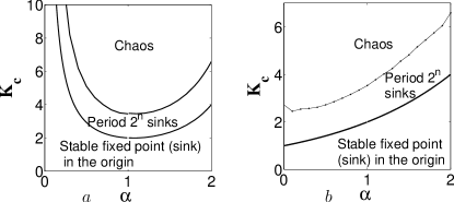
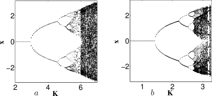
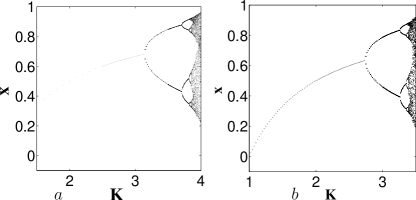
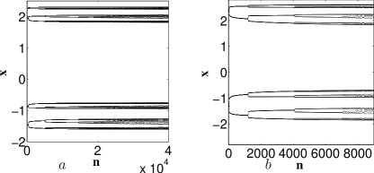
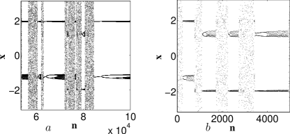
Properties of the fractional difference Caputo Standard ฮฑ๐›ผ\alphaFM were investigated in detail in Edelman (2014a) (see also Sec.ย 3 in Edelman (2014b). Qualitatively, properties of the fractional difference and fractional maps (maps with falling factorial- and power-law memory) are similar. The similarity reveals itself in the dependence of systemsโ€™ properties on the memory (ฮฑ๐›ผ\alpha) and nonlinearity (K๐พK) parameters (bifurcation diagrams, see Figs.ย 1,ย 2,ย andย 3), power-law convergence to attractors, non-uniqueness of solutions (intersection of trajectories and overlapping of attractors), and cascade of bifurcations and intermittent cascade of bifurcations type behaviors (see Figs.ย 4ย andย 5).

The differences of the properties of the falling factorial-law memory maps from the power-law memory maps are the results of the differences in weights of the recent (with $(n-j)/n<<1$) values of the mapsโ€™ variables at the time instants $t_{j}$ in the definition of the present values at time $t_{n}$ and are significant when $\alpha\in(0,1)$ (especially when $\alpha\rightarrow+0$), see Fig.ย 1.

{ack}

The author acknowledges support from the Joseph Alexander Foundation, Yeshiva University. The author expresses his gratitude to E. Hameiri, H. Weitzner, and G. Ben Arous for the opportunity to complete this work at the Courant Institute and to V. Donnelly for technical help.

References

  • Agarwal (2000) Agarwal, R. (2000). Difference equations and inequalities. Marcel Dekker, New York.
  • Anastassiou (2009) Anastassiou, G. (2009). Discrete fractional calculus and inequalities. http://arxiv.org/abs/0911.3370.
  • Atici and Eloe (2009) Atici, F. and Eloe, P. (2009). Initial value problems in discrete fractional calculus. Proc.Am.Math.Soc., 137, 981โ€“989.
  • Chen etย al. (2011) Chen, F., Luo, X., and Zhou, Y. (2011). Existence results for nonlinear fractional difference equation. Adv.Differ.Eq., 2011, 713201.
  • Chirikov (1979.) Chirikov, B. (1979.). A universal instability of many dimensional oscillator systems. Phys. Rep., 52, 263โ€“379.
  • Edelman (2011) Edelman, M. (2011). Fractional standard map: Riemann-liouville vs. caputo. Commun. Nonlin. Sci. Numer. Simul., 16, 4573โ€“4580.
  • Edelman (2013a) Edelman, M. (2013a). Fractional maps and fractional attractors. part i: $\alpha$-families of maps. Discontinuity, Nonlinearity, and Complexity, 1, 305โ€“324.
  • Edelman (2013b) Edelman, M. (2013b). Universal fractional map and cascade of bifurcations type attractors. Chaos, 23, 033127.
  • Edelman (2014a) Edelman, M. (2014a). Caputo standard $\alpha$-family of maps: fractional difference vs. fractional. Phys. Lett. A (submitted).
  • Edelman (2014b) Edelman, M. (2014b). Fractional maps and fractional attractors. part ii: fractional difference $\alpha$-families of maps. arXiv:1404.4906v2.
  • Edelman (2014c) Edelman, M. (2014c). Fractional maps as maps with power-law memory. In A.ย Afraimovich, A.ย Luo, and X.ย Fu (eds.), Nonlinear dynamics and complexity, 79โ€“120. Springer, New York.
  • Edelman and Taieb (2013) Edelman, M. and Taieb, L. (2013). New types of solutions of non-linear fractional differential equations. In A.ย Almeida, L.ย Castro, and F.O. Speck (eds.), Advances in Harmonic Analysis and Operator Theory; Series: Operator Theory: Advances and Applications, volume 229, 139โ€“155. Springer, Basel.
  • Edelman and Tarasov (2009) Edelman, M. and Tarasov, V.E. (2009). Fractional standard map. Phys. Lett. A, 374, 279โ€“285.
  • Gray and Zhang (1988) Gray, H. and Zhang, N.F. (1988). On a new definition of the fractional difference. Math. Comput., 50, 513โ€“529.
  • Kilbas etย al. (2006) Kilbas, A., Srivastava, H., and Trujillo, J. (2006). Theory and application of fractional differential equations. Elsevier, Amsterdam.
  • Lalescu (2010) Lalescu, C. (2010). Patterns in the sine map bifurcation diagram. arXiv:1011.6552.
  • Lichtenberg and Lieberman (1992) Lichtenberg, A. and Lieberman, M. (1992). Regular and chaotic dynamics. Springer, Berlin.
  • May (1976) May, R. (1976). Simple mathematical models with very complicated dynamics. Nature, 261, 459โ€“467.
  • Miller and Ross (1989) Miller, K. and Ross, B. (1989). Fractional difference calculus. In H.ย Srivastava and S.ย Owa (eds.), Univalent functions, fractional calculus, and their applications, 139โ€“151. Ellis Howard, Chichester, 1st edition.
  • Podlubny (1999) Podlubny, I. (1999). Fractional Differential Equations. Academic Press, San Diego.
  • Samko etย al. (1993) Samko, S., Kilbas, A., and Marichev, O. (1993). fractional integrals and derivatives theory and applications. Gordon and Breach, New York.
  • Stanislavsky (2006) Stanislavsky, A. (2006). Long-term memory contribution as applied to the motion of discrete dynamical system. Chaos, 16, 043105.
  • Tarasov (2009a) Tarasov, V. (2009a). Differential equations with fractional derivative and universal map with memory. J. Phys. A, 42, 465102.
  • Tarasov (2009b) Tarasov, V. (2009b). Discrete map with memory from fractional differential equation of arbitrary positive order. J. Math. Phys., 50, 122703.
  • Tarasov (2011) Tarasov, V. (2011). Fractional dynamics: application of fractional calculus to dynamics of particles, fields, and media. Springer, New York.
  • Tarasov and Zaslavsky (2008) Tarasov, V. and Zaslavsky, G. (2008). Fractional equations of kicked systems and discrete maps. J. Phys. A, 41, 435101.
  • Wu and Baleanu (2014) Wu, G.C. and Baleanu, D. (2014). Discrete fractional logistic map and its chaos. Nonlin. Dyn., 75, 283โ€“287.
  • Wu etย al. (2014) Wu, G.C., Baleanu, D., and Zeng, S.D. (2014). Discrete chaos in fractional sine and standard maps. Phys. Lett. A, 378, 484โ€“487.
  • Zaslavsky (2008) Zaslavsky, G. (2008). Hamiltonian chaos and fractional dynamics. Oxford University Press, Oxford.