iPiano: Inertial Proximal Algorithm for Non-convex Optimization
Abstract
In this paper we study an algorithm for solving a minimization problem composed of a differentiable (possibly non-convex) and a convex (possibly non-differentiable) function. The algorithm iPiano combines forward-backward splitting with an inertial force. It can be seen as a non-smooth split version of the Heavy-ball method from Polyak. A rigorous analysis of the algorithm for the proposed class of problems yields global convergence of the function values and the arguments. This makes the algorithm robust for usage on non-convex problems. The convergence result is obtained based on the Kurdyka-Łojasiewicz inequality. This is a very weak restriction, which was used to prove convergence for several other gradient methods. First, an abstract convergence theorem for a generic algorithm is proved, and, then iPiano is shown to satisfy the requirements of this theorem. Furthermore, a convergence rate is established for the general problem class. We demonstrate iPiano on computer vision problems: image denoising with learned priors and diffusion based image compression.
keywords:
non-convex optimization, Heavy-ball method, inertial forward-backward splitting, Kurdyka-Łojasiewicz inequality, proof of convergence1 Introduction
The gradient method is certainly one of the most fundamental but also one of the most simple algorithms to solve smooth convex optimization problems. In the last decades, the gradient method has been modified in many ways. One of those improvements is to consider so-called multi-step schemes [38, 35]. It has been shown that such schemes significantly boost the performance of the plain gradient method. Triggered by practical problems in signal processing, image processing and machine learning, there has been an increased interest in so-called composite objective functions, where the objective function is given by the sum of a smooth function and a non-smooth function with an easy to compute proximal map. This initiated the development of the so-called proximal gradient or forward-backward method [28], that combines explicit (forward) gradient steps w.r.t. the smooth part with proximal (backward) steps w.r.t. the non-smooth part.
In this paper, we combine the concepts of multi-step schemes and the proximal gradient method to efficiently solve a certain class of non-convex, non-smooth optimization problems. Although, the transfer of knowledge from convex optimization to non-convex problems is very challenging, it aspires to find efficient algorithms for certain non-convex problems. Therefore, we consider the subclass of non-convex problems
where is a convex (possibly non-smooth) and is a smooth (possibly non-convex) function. The sum comprises non-smooth, non-convex functions. Despite the non-convexity, the structure of being smooth and being convex makes the forward-backward splitting algorithm well-defined. Additionally, an inertial force is incorporated into the design of our algorithm, which we termed iPiano. Informally, the update scheme of the algorithm that will be analyzed is
where and are the step size parameters. The term is referred as forward step, as inertial term, and as backward or proximal step.
For the proximal step is the identity and the update scheme is usually referred as Heavy-ball method. This reduced iterative scheme is an explicit finite differences discretization of the so-called Heavy-ball with friction dynamical system
It arises when Newton’s law is applied to a point subject to a constant friction (of the velocity ) and a gravity potential . This explains the naming “Heavy-ball method” and the interpretation of as inertial force.
Setting results in the forward-backward splitting algorithm, which has the nice property that in each iteration the function value decreases. Our convergence analysis reveals that the additional inertial term prevents our algorithm from monotonically decreasing the function values. Although this may look like a limitation on first glance, demanding monotonically decreasing function values anyway is too strict as it does not allow for provably optimal schemes. We refer to a statement of Nesterov [35]: “In convex optimization the optimal methods never rely on relaxation. Firstly, for some problem classes this property is too expensive. Secondly, the schemes and efficiency estimates of optimal methods are derived from some global topological properties of convex functions”111Relaxation is to be interpreted as the property of monotonically decreasing function values in this context. Topological properties should be associated with geometrical properties.. The negative side of better efficiency estimates of an algorithm is usually the convergence analysis. This is even true for convex functions. In case of non-convex and non-smooth functions, this problem becomes even more severe.
Contributions
Despite this problem, we can establish convergence of the sequence of function values for the general case, where the objective function is only required to be a composition of a convex and a differentiable function. Regarding the sequence of arguments generated by the algorithm, existence of a converging subsequence is shown. Furthermore, we show that each limit point is a critical point of the objective function.
To establish convergence of the whole sequence in the non-convex case is very hard. However, with slightly more assumptions to the objective, namely that it satisfies the Kurdyka-Łojasiewicz inequality [30, 31, 26], several algorithms have been shown to converge [14, 5, 3, 4]. In [5] an abstract convergence theorem for descent methods with certain properties is proved. It applies to many algorithms. However, it can not be used for our algorithm. Based on their analysis, we prove an abstract convergence theorem for a different class of descent methods, which applies to iPiano. By verifying the requirements of this abstract convergence theorem, we manage to also show such a strong convergence result. From a practical point of view of image processing, computer vision, or machine learning, the Kurdyka-Łojasiewicz inequality is almost always satisfied. For more details about properties of Kurdyka-Łojasiewicz functions and a taxonomy of functions that have this property, we refer to [5, 10, 26].
The last part of the paper is devoted to experiments. We exemplarily present results on computer vision tasks, such as denoising and image compression, and show that entering the staggering world of non-convex functions pays off in practice.
2 Related Work
Forward-backward splitting
In convex optimization, splitting algorithms usually originate from the proximal point algorithm [39]. It is a very general algorithm, and results on its convergence affect many other algorithms. Practically, however, computing one iteration of the algorithm can be as hard as the original problem. Among the strategies to tackle this problem are splitting approaches like Douglas-Rachford [28, 18], several primal-dual algorithms [12, 37, 23], and forward-backward splitting [28, 16, 7, 35]; see [15] for a survey.
Especially the forward-backward splitting schemes seem to be appealing to generalize to non-convex problems. This is due to their simplicity and the existence of simpler formulations in some special cases like, for example, the gradient projection method, where the backward-step is the projection onto a set [27, 22]. In [19] the classical forward-backward algorithm, where the backward step is the solution of a proximal term involving a convex function, is studied for a non-convex problem. In fact, the same class of objective functions as in the present paper is analyzed. The algorithm presented here comprises the algorithm from [19] as a special case. Also Nesterov [36] briefly accounts this algorithm in a general setting. Even the reverse setting is generalized in the non-convex setting [5, 11], namely where the backward-step is performed on a non-smooth non-convex function.
As the amount of data to be processed is growing and algorithms are supposed to exploit all the data in each iteration, inexact methods become interesting, though we do not consider erroneous estimates in this paper. Forward-backward splitting schemes also seem to work for non-convex problems with erroneous estimates [44, 43]. A mathematical analysis of inexact methods can be found, e.g., in [14, 5], but with the restriction that the method is explicitly required to decrease the function values in each iteration. The restriction comes with significantly improved results with regard of the convergence of the algorithm. The algorithm proposed in this paper provides strong convergence results, although it does not require the function values to decrease.
Optimization with inertial forces
In his seminal work [38], Polyak investigates multi-step schemes to accelerate the gradient method. It turns out that a particularly interesting case is given by a two-step algorithm, which has been coined the Heavy-ball method. The name of the method is because it can be interpreted as an explicit finite differences discretization of the so-called Heavy-ball with friction dynamical system. It differs from the usual gradient method by adding an inertial term that is computed by the difference of the two preceding iterations. Polyak showed that this method can speed up convergence in comparison to the standard gradient method, while the cost of each iteration stays basically unchanged.
The popular accelerated gradient method of Nesterov [35] obviously shares some similarities with the Heavy-ball method, but it differs from it in one regard: while the Heavy-ball method uses gradients based on the current iterate, Nesterov’s accelerated gradient method evaluates the gradient at points that are extrapolated by the inertial force. On strongly convex functions, both methods are equally fast (up to constants), but Nesterov’s accelerated gradient method converges much faster on weakly convex functions [17].
The Heavy-ball method requires knowledge about the function parameters (Lipschitz constant of the gradient and the modulus of strong convexity) to achieve the optimal convergence rate, which can be seen as a disadvantage. Interestingly, the conjugate gradient method for minimizing strictly convex quadratic problems can be expressed as Heavy-ball method. Hence, it can be seen as a special case of the Heavy-ball method for quadratic problems. In this special case, no additional knowledge is required about the function parameters, as the algorithm parameters are computed online.
The Heavy-ball method was originally proposed for minimizing differentiable convex functions, but it has been generalized in different ways. In [45], it has been generalized to the case of smooth non-convex functions. It is shown that, by considering an appropriate Lyapunov objective function, the iterations are attracted by the connected components of stationary points. In Section 4 it will become evident that the non-convex Heavy-ball method is a special case of our algorithm, and also the convergence analysis of [45] shows some similarities to ours.
3 An abstract convergence result
3.1 Preliminaries
We consider the Euclidean vector space of dimension and denote the standard inner product by and the induced norm by . Let be a proper lower semi-continuous function.
Definition 1 (effective domain, proper).
The (effective) domain of is defined by . The function is called proper, if is nonempty.
In order to give a sound description of the first order optimality condition for a non-convex non-smooth optimization problem, we have to introduce the generalization of the subdifferential for convex functions.
Definition 2 (Limiting-subdifferential).
The limiting-subdifferential (or simply subdifferential) is defined by (see [40, Def. 8.3])
| (1) |
which makes use of the Fréchet subdifferential defined by
when and by else.
The domain of the subdifferential is .
In what follows, we will consider the problem of finding a critical point of , which is characterized by the necessary first-order optimality condition .
We state the definition of the Kurdyka-Łojasiewicz property from [4].
Definition 3 (Kurdyka-Łojasiewicz property).
-
1.
The function has the Kurdyka-Łojasiewicz property at , if there exist , a neighborhood of and a continuous concave function such that , , for all it is , and for all the Kurdyka-Łojasiewicz inequality holds, i.e.,
-
2.
If the function satisfies the Kurdyka-Łojasiewicz inequality at each point of , it is called KL function.
Roughly speaking, this condition says that we can bound the subgradient of a function from below by a reparametrization of its function values. In the smooth case, we can also say that up to a reparametrization the function is sharp, meaning that any non-zero gradient can be bounded away from . This is sometimes called a desingularization. It has been shown in [4] that a proper lower semi-continuous extended valued function always satisfies this inequality at each non-stationary point. For more details and other interpretations of this property, also for different formulations, we refer to [10].
A big class of functions that have the KL-property is given by real semi-algebraic functions [4]. Real semi-algebraic functions are defined as functions whose graph is a real semi-algebraic set.
Definition 4 (real semi-algebraic set).
A subset of is semi-algebraic, if there exists a finite number of real polynomials such that
3.2 Inexact descent convergence result for KL functions
In the following, we prove an abstract convergence result for a sequence in , , , satisfying certain basic conditions, . For convenience we use the abbreviation for . We fix two positive constants and and consider a proper lower semi-continuous function . Then, the conditions we require for are
-
(H1)
For each , it holds
-
(H2)
For each , there exists such that
-
(H3)
There exists a subsequence such that
Based on these conditions, we derive the same convergence result as in [5]. The statements and proofs of the subsequent results follow the same ideas as [5]. We modified the involved calculations according to our conditions H1, H2, and H3.
Remark 1.
Remark 2.
Lemma 5.
Let be a proper lower semi-continuous function which satisfies the Kurdyka-Łojasiewicz property at some point . Denote by , and the objects appearing in Definition 3 of the KL property at . Let be such that with , where .
Furthermore, let be a sequence satisfying Conditions H1, H2, and
| (2) |
Moreover, the initial point is such that and
| (3) |
Then, the sequence satisfies
| (4) |
converges to a point such that . If, additionally, Condition H3 is satisfied, then and .
Proof.
The key points of the proof are the facts that for all :
| (5) | |||
| (6) |
Let us first see that is well-defined. By Condition H1, is non-increasing, which shows . Combining this with (2) implies .
As for the set is nonempty (see Condition H2) every belongs to . For notational convenience, we define
Now, we want to show that for holds: if and , then
| (7) |
Obviously, we can assume that (otherwise it is trivial), and therefore H1 and (2) imply . The KL inequality shows and H2 shows . Since , using KL inequality and H2, we obtain
As is concave and increasing (), Condition H1 and (2) yield
Combining both inequalities results in
which by applying establishes (7).
As (2) does only imply , , we can not use (7) directly for the whole sequence. However, (5) and (6) can be shown by induction on . For , (2) yields and . From Condition H1 with , and , we infer
| (8) |
which combined with (3) leads to
and therefore . Direct use of (7) with shows that (6) holds with .
Suppose (5) and (6) are satisfied for . Then, using the triangle inequality and (6), we have
which shows, using and (3), that . As a consequence (7), with , can be added to (6) and we can conclude (6) with . This shows the desired induction on .
Now, the finiteness of the length of the sequence , i.e., , is a consequence of the following estimation, which is implied by (6),
Therefore, converges to some as , and converges to . As is concave, is decreasing. Using this and Condition H2 yields and . Suppose we have , then KL-inequality reads for all , which contradicts .
Note that, in general, is not a critical point of , because the limiting subdifferential requires as . When the sequence additionally satisfies Condition H3, then , and is a critical point of , because . ∎
Remark 3.
The next corollary and the subsequent theorem follow as in [5] by replacing the calculation with our conditions.
Proof.
By Condition H1, for , we have
Using the triangle inequality on shows that , which implies (2) and concludes the proof. ∎
The work that is done in Lemma 5 and Corollary 6 allows us to formulate an abstract convergence theorem for sequences satisfying the Conditions H1, H2, and H3. It follows, with a few modifications, as in [5].
Theorem 7 (Convergence to a critical point).
Let be a proper lower semi-continuous function and a sequence that satisfies H1, H2, and H3. Moreover, let have the Kurdyka-Łojasiewicz property at the cluster point specified in H3.
Then, the sequence has finite length, i.e., , and converges to as , where is a critical point of .
Proof.
By Condition H3, we have and for a subsequence . This, together with the non-decreasingness of (by Condition H1), imply that and for all . The KL-property around states the existence of quantities , , and as in Definition 3. Let be such that and . Shrink such that (if necessary). As is continuous, there exists such that for all and
Then, the sequence defined by satsifies the conditions in Corollary 6, which concludes the proof. ∎
4 The proposed algorithm - iPiano
4.1 The optimization problem
We consider a structured non-smooth non-convex optimization problem with a proper lower semi-continuous extended valued function , :
| (9) |
which is composed of a -smooth (possibly non-convex) function with -Lipschitz continuous gradient on , , and a convex (possibly non-smooth) function . Furthermore, we require to be coercive, i.e., implies , and bounded from below by some value .
The proposed algorithm, which is stated in Subsection 4.3, seeks for a critical point of , which is characterized by the necessary first-order optimality condition . In our case, this is equivalent to
This equivalence is explicitly verified in the next subsection, where we collect some details and state some basic properties, which are used in the convergence analysis in Subsection 4.5.
4.2 Preliminaries
Consider the function first. It is required to be -smooth with -Lipschitz continuous gradient on , i.e., there exists a constant such that
| (10) |
This directly implies that is a non-empty convex set, as . This property of plays a crucial role in our convergence analysis due to the following lemma (stated as in [5]).
Lemma 8 (descent lemma).
Let be a -function with -Lipschitz continuous gradient on . Then for any it holds that
| (11) |
Proof.
See for example [35]. ∎
We assume that the function is a proper lower semi-continuous convex function with an efficient to compute proximal map.
Definition 9 (proximal map).
Let be a proper lower semi-continuous convex function. Then, we define the proximal map
where is a given parameter, is the identity map, and .
An important (basic) property that the convex function contributes to the convergence analysis is the following:
Lemma 10.
Let be a proper lower semi-continuous convex function, then it holds for any , that
| (12) |
Proof.
This result follows directly from the convexity of . ∎
Finally, consider the optimality condition more in detail. The following proposition proves the equivalence to . The proof is mainly based on Definition 2 of the limiting-subdifferential.
Proposition 11.
Let , , and be like before, i.e., let with continuously differentiable and convex. Sometimes, is then called a -perturbation of a convex function. Then, for holds
Proof.
We first prove “”. Let , i.e., there is a sequence such that , , and , where . We want to show that . As and , we have
It remains to show that . First, remember that is superadditive, i.e., for two sequences , in it is . However, convergence of implies . This fact and again thanks to , we conclude
where and are over . Therefore, .
The other inclusion “” is trivial.
∎
As a consequence, a critical point can also be characterized by the following definition.
Definition 12 (proximal residual).
Let and be as afore. Then, we define the proximal residual
It can be easily seen that is equivalent to and , which is the first-order optimality condition. The proximal residual is defined with respect to a fixed step size of . The rationale behind this becomes obvious when is the indicator function of a convex set. In this case, a small residual could be caused by small step sizes as the reprojection onto the convex set is independent of the step size.
4.3 The generic algorithm
In this paper, we propose an algorithm, iPiano, with the generic formulation in Algorithm 1. It is a forward-backward splitting algorithm incorporating an inertial force. In the forward step, determines the step size in the direction of the gradient of the differentiable function . The step in gradient direction is aggregated with the inertial force from the previous iteration weighted by . Then, the backward step is the solution of the proximity operator for the function with the weight .
Algorithm 1.
inertial proximal algorithm
for non-convex optimization (iPiano)
•
Initialization: Choose a starting point and set . Moreover, define sequences of step size parameter and .
•
Iterations : Update
(13)
4.4 Rules for choosing the step size
In this subsection, we propose several strategies for choosing the step sizes. This will make it easier to implement the algorithm. One may choose among the following variants of step size rules depending on the knowledge about the objective function.
Constant step size scheme
The most simple one, which requires most knowledge about the objective function, is outlined in Algorithm 2. All step size parameters are chosen a priori and are constant.
Algorithm 2.
inertial proximal algorithm for
non-convex optimization with constant parameter (ciPiano)
•
Initialization: Choose , set , where is the Lipschitz constant of ,
choose , and set .
•
Iterations : Update as follows:
(14)
Remark 4.
Observe that our law on is equivalent to the law found in [45] for minimizing a smooth non-convex function. Hence, our result can be seen as an extension of their work to the presence of an additional non-smooth convex function.
Backtracking
The case where we have only limited knowledge about the objective function occurs more frequently. It can be very challenging to estimate the Lipschitz constant of beforehand. Using backtracking the Lipschitz constant can be estimated automatically. A sufficient condition that the Lipschitz constant at iteration to must satisfy is
| (15) |
Although, there are different strategies to determine , the most common one is by defining an increment variable and looking for minimal satisfying (15). Sometimes, it is also feasible to decrease the estimated Lipschitz constant after a few iterations. A possible strategy is as follows: if , then search for the minimal satisfying (15).
In Algorithm 3 we propose an algorithm with variable step sizes. Any strategy for estimating the Lipschitz constant may be used. When changing the Lipschitz constant from one iteration to another, all step size parameters must be adapted. The rules for adapting the step sizes will be justified during the convergence analysis in Subsection 4.5.
Algorithm 3.
inertial proximal algorithm for
non-convex optimization with backtracking (biPiano)
•
Initialization: Choose with close to (e.g. ), and
and set .
•
Iterations : Update as follows:
(16)
where satisfies (15) and
Lazy backtracking
Algorithm 4 presents another alternative of Algorithm 1. It is related to Algorithm 2 and 3 in the following way. Algorithm 4 makes use of the Lipschitz continuity of in the sense that the Lipschitz constant is always finite. As a consequence, using backtracking with only increasing Lipschitz constants, after a finite number of iterations the estimated Lipschitz constant will not change anymore, and starting from this iteration the constant step size rules as in Algorithm 2 are applied. Using this strategies, the results that will be proved in the convergence analysis are satisfied only as soon as the Lipschitz constant is high enough and does not change anymore.
Algorithm 4.
non-monotone inertial proximal algorithm
for non-convex optimization with backtracking (nmiPiano)
•
Initialization: Choose , , , and
and set .
•
Iterations : Update as follows:
(17)
where is minimal
satisfying
(18)
and .
General rule of choosing the step sizes
Algorithm 5 defines the general rules that the step size parameters must satisfy.
Algorithm 5.
inertial proximal algorithm
for non-convex optimization (iPiano)
•
Initialization: Choose close to , and set .
•
Iterations : Update
(19)
where is the local Lipschitz constant satisfying
(20)
and , are chosen such that defined by
(21)
and is monotonically decreasing.
It contains the Algorithms 2, 3, and 4 as special instances. This is easily verified for Algorithms 2 and 4. For Algorithm 3 the step size rules are derived from the proof of Lemma 13.
As Algorithm 5 is the most general one, now, let us analyze the behavior of this algorithm.
4.5 Convergence analysis
In all what follows, let be the sequence generated by Algorithm 5 and with parameters satisfying the algorithm’s requirements. Furthermore, for a more convenient notation we abbreviate , , and . Note, that for it is .
Let us first verify that the algorithm makes sense. We have to show that the requirements to the parameters are not contradictory, i.e., that it is possible to choose a feasible set of parameters. In the following Lemma, we will only show existence of such a parameter set, however, the proof helps us to formulate specific step size rules.
Lemma 13.
For all , there are , , and . Furthermore, given , there exists a choice of parameter and such that additionally is monotonically decreasing.
Proof.
By the algorithm’s requirements it is
The upper bound for and come from rearranging
to and
, respectively.
The last statement follows by incorporating the descent property of .
Let be chosen initially. Then, the decent property of
requires one of the equivalent statements
to be true. An upper bound on is obtained by
The only thing that remains to show is that there exists and such that these two relations are fulfilled. Consider the condition for a non-negative gap between the upper and lower bound for
Defining , it is easily verified that there exists satisfying the equivalent condition
| (22) |
As a consequence, the existence of a feasible follows, and the decent property for holds. ∎
In the following proposition, we state a result which will be very useful. Although, iPiano does not imply a descent property of the function values, we construct a majorizing function that enjoys a monotonically descent property. This function reveals the connection to the Lyapunov direct method for convergence analysis as used in [45].
Proposition 14.
-
(a)
The sequence is monotonically decreasing and thus converging. In particular, it holds
(23) -
(b)
It holds and, thus, .
Proof.
-
(a)
From (19) it follows that
Now using and in (11) and (12) and summing both inequalities it follows that
where the second line follows from for vectors . Then, a simple rearrangement of the terms shows
which establishes (23) as is monotonically decreasing. Obviously, the sequence is monotonically decreasing if and only if , which is true by the algorithm’s requirements. By assumption, is bounded from below by some constant , hence converges.
-
(b)
Summing up (23) from yields (note that )
Letting tend to and remembering that holds implies the statement.
∎
Remark 5.
The function is a Lyapunov function for the dynamical system of described by the Heavy-ball method. It corresponds to a discretized version of the kinetic energy of the Heavy-ball with friction.
In the following theorem, we state our general convergence results about Algorithm 5.
Theorem 15.
-
(a)
The sequence converges.
-
(b)
There exists a converging subsequence .
-
(c)
Any limit point is a critical point of (9) and as .
Proof.
- (a)
- (b)
-
(c)
To show that each limit point is a critical point of (9) recall that the subdifferential (1) is closed [40]. Define
Then, the sequence . Furthermore, it holds and due to Proposition 14(b), the Lipschitz continuity of , and
it holds . It remains to show that . By the closure property of the subdifferential it is , which means that is a critical point of .
The continuity statement about the limiting process as follows by the lower semi-continuity of , the existence , and the convexity property in Lemma 10
The first equality holds because the subadditivity of becomes an equality when the limit exists for one of the two summed sequences222In general, the existence of is not guaranteed. Compared to the general case, additionally is known here., here it exists . Moreover, as is differentiable it is also continuous, thus . This implies .
∎
Remark 6.
The convergence properties shown in Theorem 15 should be the basic requirement of any algorithm. Very loosely speaking, it states that the algorithm ends up in a meaningful solution. It allows us to formulate stopping conditions, e.g., the residual between successive function values.
Now, using Theorem 7, we can verify the convergence of the sequence generated by Algorithm 5. We assume that after a finite number of steps the sequence is constant and consider the sequence starting from this iteration (again denoted by ). For example, if is determined relative to the Lipschitz constant, then as the Lipschitz constant can be assumed constant after a finite number of iterations, is also constant starting from this iteration.
Theorem 16 (Convergence of iPiano to a critical point).
Let be generated by Algorithm 5, and let for all . Then, the sequence satisfies H1, H2, and H3 for the function , .
Moreover, if has the Kurdyka-Łojasiewicz property at a cluster point , then the sequence has finite length, as , and is a critical point of , hence is a critical point of .
Proof.
First, we verify that the Assumptions H1, H2, and H3 are satisfied. We consider the sequence for all and the proper lower semi-continuous function .
-
•
Condition H1 is proved in Proposition 14(a) with .
-
•
To proof Condition H2, consider with and . The Lipschitz continuity of and using (19) to specify an element from imply
As and , setting verifies condition H2, i.e., .
- •
Now, the abstract convergence Theorem 7 concludes the proof. ∎
The next corollary makes use of the fact that semi-algebraic functions (Definition 4) have the Kurdyka-Łojasiewicz property.
Corollary 17 (Convergence of iPiano for semi-algebraic functions).
Let be a semi-algebraic function. Then, is also semi-algebraic. Furthermore, let , , be as in Theorem 16. Then the sequence has finite length, as , and is a critical point of .
Proof.
As and are semi-algebraic, is semi-algebraic and has the KL property. Then, Theorem 16 concludes the proof. ∎
4.6 Convergence rate
In the following, we are interested in determining a convergence rate with respect to the proximal residual from Definition 12. Since all preceding estimations are according to we establish the relation to first. The following lemmas about the monotonicity and the non-expansiveness of the proximity operator turn out to be very useful for that. Coarsely speaking, Lemma 18 states that the residual is sub-linearly increasing. Lemma 19 formulates a standard property of the proximal operator.
Lemma 18 (Proximal monotonicity).
Let , and . Define the functions
and
Then, is a decreasing function of , and increasing in .
Lemma 19 (Non-expansiveness).
Let be a convex function and , then, for all we obtain the non-expansiveness of the proximity operator
| (24) |
Proof.
It is a well-known fact. See for example [6]. ∎
The two preceding lemmas allow us to establish the following relation.
Lemma 20.
We have the following bound:
| (25) |
Proof.
First, we observe the relations and , which are based on Lemma 18. Then, invoking the non-expansiveness of the proximity operator (Lemma 19) we obtain
| (26) |
This allows us to compute the following lower bound
where the first inequality arises from adding zero and using (26), the second uses the triangle inequality, the next one applies Lemma 18 and . Now, summing both sides from and using the statement easily follows. ∎
Next, we prove a global convergence rate for and the residuum of the algorithm. The residuum provides an error measure of being a fixed point and hence a critical point of the problem. We first define the error to be the smallest squared norm of successive iterates and, analogously, the error
Theorem 21.
Algorithm 5 guarantees that for all
Proof.
Remark 7.
The convergence rate for the squared norm of our error measures is equivalent to stating a convergence rate for the error in the norm.
Remark 8.
A similar result can be found in [36] for the case .
5 Numerical experiments
In all the following experiments, let be vectors of dimension , where depends on the respective problem. In the case of an image is the number of pixels.
5.1 Ability to overcome spurious stationary points
Let us present some of the qualitative properties of the proposed algorithm. For this, we consider to minimize the following simple problem
| (27) |
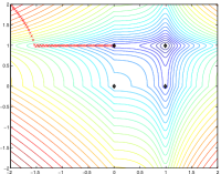
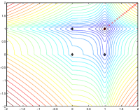
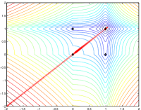
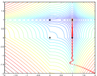
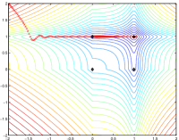
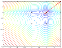
where is the unknown vector, is some given vector, and are some free parameters. A contour plot and the energy landscape of in the case of , , , and is depicted in Figure 1. It turns out that the function has four stationary points, i.e. points , such that . These points are marked by small black diamonds.
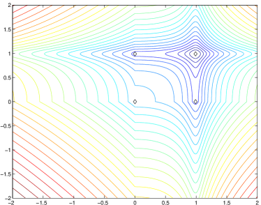
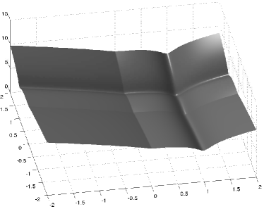
Clearly the function is non-convex but has a Lipschitz continuous gradient with components
The Lipschitz constant of is easily computed as . The function is non-smooth but convex and the proximal operator with respect to is given by the well-known shrinkage operator
| (28) |
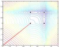
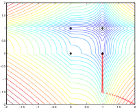
where all operations are understood component-wise. Let us test the performance of the proposed algorithm on the example shown in Figure 1. We set . Figure 2 shows the results of using the iPiano algorithm for different settings of the extrapolation factor . We observe that iPiano with is strongly attracted by the closest stationary points while switching on the inertial term can help to overcome the spurious stationary points. The reason for this desired property is that while the gradient might vanish at some points, the inertial term is still strong enough to drive the sequence out of the stationary region. Clearly, there is no guarantee that iPiano always avoids spurious stationary points. iPiano is not designed to find the global optimum. However, our numerical experiments suggest that in many cases, iPiano finds lower energies than the respective algorithm without inertial term. A similar observation about the Heavy-ball method is described in [8].
5.2 Image processing applications
It is well-known that non-convex regularizers are better models for many image processing and computer vision problems, see e.g. [9, 21, 25, 41]. However, convex models are still preferred over non-convex ones, since they can be efficiently optimized using convex optimization algorithms. In this section, we demonstrate the applicability of the proposed algorithm to solve a class of non-convex regularized variational models. We present examples for natural image denoising, and linear diffusion based image compression. We show that iPiano can be easily adapted to all these problems and yields state-of-the-art results.
5.2.1 Student-t regularized image denoising
In this subsection, we investigate the task of natural image denoising. For this we exploit an optimized MRF (Markov random field) model, which is learned in following [13], and make use of the iPiano algorithm to solve it. In order to evaluate the performance of iPiano, we compare it to the well-known bound constrained limited memory quasi Newton method (L-BFGS) [29] 333We make use of the implementation distributed at http://www.cs.toronto.edu/~liam/software.shtml.. As an error measure, we use the energy difference
| (29) |
where is the energy of the current iteration and is the energy of the true solution. Clearly, this error measure makes sense only when different algorithms can achieve the same true energy which is in general wrong for non-convex problems. In our image denoising experiments, however, we find, that all tested algorithms find the same solution, independent of the initialization. This can be explained by the fact that the learning procedure [13] also delivers models that are relatively easy to optimize, since otherwise they would have resulted in a bad training error. In order to compute a true energy , we run the iPiano algorithm with a proper (e.g., ) for enough iterations (1000 iterations). We run all the experiments in Matlab on a 64-bit Linux server with 2.53GHz CPUs.
The MRF image denoising model based on learned filters is formulated as
| (30) |
where and denote the sought solution and the noisy input image respectively, is the non-convex penalty function, , are learned, linear operators with the corresponding weights , and is the number of the filters. The linear operators are implemented as 2D convolutions of the image with small (e.g. ) filter kernels , i.e. . The function is the data term, which depends on the respective problem. In the case of Gaussian noise, is given as
and for the impulse noise (e.g., salt & pepper noise), is given as
The parameter is used to define the tradeoff between regularization and data fitting.
In this paper, we consider the following non-convex penalty function, which is derived from the Student-t distribution:
| (31) |
Concerning the filters , for the model (MRF-), we make use of the filters learned in [13], by using a bi-level learning approach. The filters are shown in Figure 3(a) together with the corresponding weights . For the MRF- denoising model, we employ the same bi-level learning algorithm to train a set of optimal filters specialized for the data term and input images degraded by salt & pepper noise. Since the bi-level learning algorithms requires a twice continuously differentiable model we replace the norm by a smooth approximation during training. The learned filters for the MRF- model together with the corresponding weights are shown in Figure 3(b).



Let us now explain how to solve (30) using the iPiano algorithm. Casting (30) in the form of (9), we see that and . Thus, we have
where and . The proximal map with respect to simply poses point-wise operations. For the case of , it is given by
and for the function , it is given by the well-known soft shrinkage operator (28), which in case of the MRF- model becomes
Now, we can make use of our proposed algorithm to solve the non-convex optimization problems. In order to evaluate the performance of iPiano, we compare it to L-BFGS. To use L-BFGS, we merely need the gradient of the objective function with respect to . For the MRF- model, calculating the gradients is straightforward. However, in the case of the MRF- model, due to the non-smooth function , we cannot directly use L-BFGS. Since L-BFGS can easily handle box constraints, we can get rid of the non-smooth function norm by introducing two box constraints.
Lemma 22.
The MRF- model can be equivalently written as the bound-constraint problem:
| (32) |
Proof.
It is well-know that the norm can be equivalently expressed as
where and the inequalities are understood pointwise. Letting , and , we find and . Substituting and back into (30) while using the above formulation of the norm yields the desired transformation. ∎
| iPiano with different | L-BFGS | ||||||||
| tol | 0.00 | 0.20 | 0.40 | 0.60 | 0.80 | 0.95 | (s) | iter. | (s) |
| 260 | 182 | 116 | 66 | 56 | 214 | 34.073 | 43 | 18.465 | |
| 372 | 256 | 164 | 94 | 67 | 257 | 40.199 | 55 | 22.803 | |
| 505 | 344 | 222 | 129 | 79 | 299 | 47.177 | 66 | 27.054 | |
| 664 | 451 | 290 | 168 | 98 | 342 | 59.133 | 79 | 32.143 | |
| 857 | 579 | 371 | 216 | 143 | 384 | 85.784 | 93 | 36.926 | |
| 1086 | 730 | 468 | 271 | 173 | 427 | 103.436 | 107 | 41.939 | |
| 1347 | 904 | 577 | 338 | 199 | 473 | 119.149 | 124 | 48.272 | |
| 1639 | 1097 | 697 | 415 | 232 | 524 | 138.416 | 139 | 53.290 | |
| 1949 | 1300 | 827 | 494 | 270 | 569 | 161.084 | 154 | 58.511 | |
| iPiano with different | L-BFGS | ||||||||
| tol | 0.00 | 0.20 | 0.40 | 0.60 | 0.80 | 0.95 | (s) | iter. | (s) |
| 390 | 272 | 174 | 96 | 64 | 215 | 43.709 | 223 | 102.383 | |
| 621 | 403 | 256 | 145 | 77 | 260 | 53.143 | 246 | 112.408 | |
| 847 | 538 | 341 | 195 | 96 | 304 | 65.679 | 265 | 121.303 | |
| 1077 | 682 | 433 | 247 | 120 | 349 | 81.761 | 285 | 130.846 | |
| 1311 | 835 | 530 | 303 | 143 | 395 | 97.060 | 298 | 136.326 | |
| 1559 | 997 | 631 | 362 | 164 | 440 | 111.579 | 311 | 141.876 | |
| 1818 | 1169 | 741 | 424 | 185 | 485 | 126.272 | 327 | 148.945 | |
| 2086 | 1346 | 853 | 489 | 208 | 529 | 142.083 | 347 | 157.956 | |
| 2364 | 1530 | 968 | 557 | 233 | 575 | 159.493 | 372 | 169.674 | |
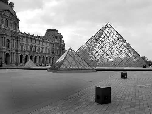
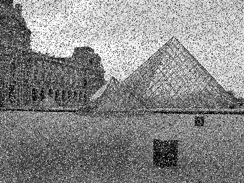
Figure 4 and Figure 5 respectively show a denoising example using the MRF- model, and the MRF- model. In both experiments, we use the iPiano version with backtracking (Algorithm 4) with the following parameter settings:
where is a free parameter to be evaluated in the experiment. In order to make use of possible larger step sizes in practice, we use a following trick: when the inequality (15) is fulfilled, we decrease the evaluated Lipschitz constant slightly by setting .
For the MRF- denoising experiments, we initialized using the noisy image itself, however, for the MRF- denoising model, we initialized using a zero image. We found that this initialization strategy usually gives good convergence behavior for both algorithms. For both denoising examples, we run the algorithms until the error decreases to a certain predefined threshold tol. We then record the required number of iterations and the run time. We summarize the results of the iPiano algorithm with different settings and L-BFGS in Table 1 and 2. From these two tables, one can draw the common conclusion that iPiano with a proper inertial term takes significantly less iterations compared to the case without inertial term, and in practice is generally a good choice.
In Table 1, one can see that the iPiano algorithm with takes slightly more iterations and run time to reach a solution of moderate accuracy (e.g., ) compared with L-BFGS. However, for high accurate solutions (e.g., ), this gap increases. For the case of the non-smooth MRF- model, the result is just the reverse. It is shown in Figure 2, that for reaching a moderately accurate solution, iPiano with consumes significantly less iterations and run time, and for the solution of high accuracy, it still can save much computation.
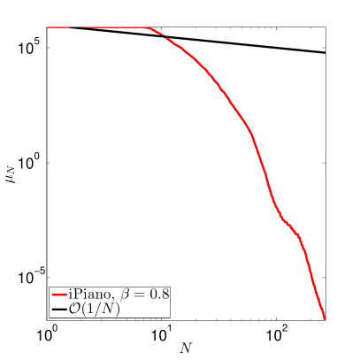
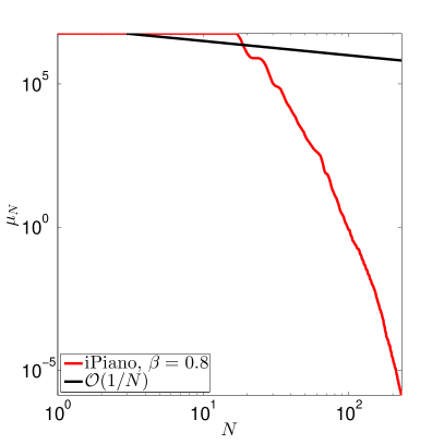
Figure6 plots the error over the number of required iterations for both the MRF- and - models using . From the plots it becomes obvious that the empirical performance of the iPiano algorithm is much better compared to the worst-case convergence rate of as provided in theorem 21.
The iPiano algorithm has an additional advantage of simplicity. The iPiano version without backtracking basically relies on matrix vector products (filter operations in the denoising examples) and simple pointwise operations. Therefore, the iPiano algorithm is well suited for a parallel implementation on GPUs which an lead to speedup factors of 20-30.
5.2.2 Linear diffusion based image compression
In this example we apply the iPiano algorithm to linear diffusion based image compression. Recent works [20, 42] have shown that image compression based on linear and non-linear diffusion can outperform the standard JPEG standard and even the more advanced JPEG 2000 standard, when the interpolation points are carefully chosen. Therefore, finding optimal data for interpolation is a key problem in the context of PDE-based image compression. There exist only few prior works for this topic, see e.g. [33, 24], and the very recent approach presented in [24] defines the state-of-the-art.
The problem of finding optimal data for homogeneous diffusion-based interpolation is formulated as the following constrained minimization problem:
| (33) | ||||
| s.t. |
where denotes the ground truth image, denotes the reconstructed image, and denotes the inpainting mask, i.e. the characteristic function of the set of points that are chosen for compressing the image. Furthermore, we denote by the diagonal matrix with the vector on its main diagonal, by the identity matrix and by the Laplacian operator. Compared to the original formulation [24], we omit a very small quadratic term , because we find it unnecessary in experiments.
Observe that if , we can multiply the constraint equation in (33) from the left by such that it becomes
where . This shows that problem (33) is in fact a reduced formulation of the bilevel optimization problem
| (34) | ||||
| s.t. |
where is the nabla operator and hence .
Problem (33) is non-convex due to the non-convexity of the equality constraint. In [24], the above problem is solved by a successive primal-dual (SPD) algorithm, which successively linearizes the non-convex constraint and solves the resulting convex problem with the first-order primal-dual algorithm [12]. The main drawback of SPD is, that it requires tens of thousands inner iterations and thousands of outer iterations to reach a reasonable solution. However, as we now demonstrate, iPiano can solve this problem with higher accuracy in 1000 iterations.
Observe that we can rewrite the problem (33) by solving from the constraints equation, which gives
where . In [32], it is shown that the is invertible as long as at least one element of is non-zero, which is the case for non-degenerate problems. Substituting back the above equation into (33), we arrive at the following optimization problem, which now only depends on the inpainting mask :
| (35) |
Casting (35) in the form of (9), we have , and . In order to minimize the above problem using iPiano, we need to calculate the gradient of with respect to . This is shown by the following lemma.
Lemma 23.
Let
then
| (36) |
Proof.
Finally, we need to compute the proximal map with respect to which is again given by a pointwise application of the shrinkage operator (28).
Now, we can make use of the iPiano algorithm to solve the problem (35). We set , which generally performs very well in practice. We additionally accelerate the SPD algorithm used in the previous work [24] by applying the diagonal preconditioning technique [37], which significantly reduces the required iterations for the primal-dual algorithm in the inner loop.
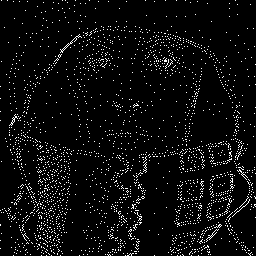
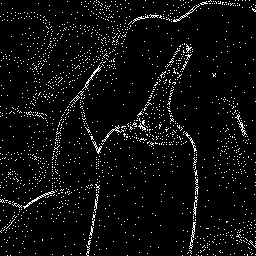
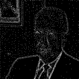
Figure 7 shows examples of finding optimal interpolation data for the three test images. Table 3 summarizes the results of two different algorithms. Regarding the reconstruction quality, we make use of the mean squared error (MSE) as an error measurement to keep consistent with previous work, which is computed by
From Table 3, one can see that the Successive PD algorithm requires iterations to converge. iPiano only needs 1000 iterations to reach already a lower energy. Note that in each iteration of the iPiano algorithm, two linear systems have to be solved. In our implementation we use the Matlab “backslash” operator which effectively exploits the strong sparseness of the systems. A lower energy basically implies that iPiano can solve the minimization problem (33) better. Regarding the final compression result, usually the result of iPiano has slightly less density, but slightly worse MSE. Following the work [33], we also consider the so-called gray value optimization (GVO) as a post-processing step to further improve the MSE of the reconstructed images.






| Test image | Algorithm | Iterations | Energy | Density | MSE | with GVO |
|---|---|---|---|---|---|---|
| trui | iPiano | 1000 | 21.574011 | 4.98% | 17.31 | 16.89 |
| SPD | 200/4000 | 21.630280 | 5.08% | 17.06 | 16.54 | |
| peppers | iPiano | 1000 | 20.631985 | 4.84% | 19.50 | 18.99 |
| SPD | 200/4000 | 20.758777 | 4.93% | 19.48 | 18.71 | |
| walter | iPiano | 1000 | 10.246041 | 4.82% | 8.29 | 8.03 |
| SPD | 200/4000 | 10.278874 | 4.93% | 8.01 | 7.72 |
6 Conclusions
In this paper, we have proposed a new optimization algorithm, which we call iPiano. It is applicable to a broad class of non-convex problems. More specifically, it addresses objective functions, which are composed as a sum of a differentiable (possibly non-convex) and a convex (possibly non-differentiable) function. The basic methodologies have been derived from the forward-backward splitting algorithm and the Heavy-ball method.
Our theoretical convergence analysis is divided into two steps. First, we have proved an abstract convergence result about inexact descent methods. Then, we analyze the convergence of iPiano. For iPiano, we have proved that the sequence of function values converges, that the subsequence of arguments generated by the algorithm is bounded, and that every limit point is a critical point of the problem. Requiring the Kurdyka-Łojasiewicz property for the objective function establishes deeper insights into the convergence behavior of the algorithm. Using the abstract convergence result, we have shown that the whole sequence converges and the unique limit point is a stationary point.
The analysis includes an examination of the convergence rate. A rough upper bound of has been found for the squared proximal residual. Experimentally, iPiano has been shown to have a much faster convergence rate.
Finally, the applicability of the algorithm has been demonstrated and iPiano achieved state-of-the-art performance. The experiments comprised denoising and image compression. In the first two experiments, iPiano helped learning a good prior for the problem. In the case of image compression, iPiano has demonstrated its use in a huge optimization problem for computing an optimal mask for a Laplacian PDE-based image compression method.
In summary, iPiano has many favorable theoretical properties, is simple and efficient. Hence, we recommend it as a standard solver for the considered class of problems.
7 Acknowledgements
We are grateful to Joachim Weickert for discussions about the image compression by diffusion problem.
References
- [1] F. Alvarez, Weak convergence of a relaxed and inertial hybrid projection-proximal point algorithm for maximal monotone operators in Hilbert space, SIAM Journal on Optimization, 14 (2003), pp. 773–782.
- [2] F. Alvarez and H. Attouch, An inertial proximal method for maximal monotone operators via discretization of a nonlinear oscillator with damping, Set-Valued Analysis, 9 (2001), pp. 3–11.
- [3] H. Attouch and J. Bolte, On the convergence of the proximal algorithm for nonsmooth functions involving analytic features, Mathematical Programming, 116 (2008), pp. 5–16.
- [4] H. Attouch, J. Bolte, P. Redont, and A. Soubeyran, Proximal alternating minimization and projection methods for nonconvex problems: An approach based on the Kurdyka-Łojasiewicz inequality, Mathematics of Operations Research, 35 (2010), pp. 438–457.
- [5] H. Attouch, J. Bolte, and B. Svaiter, Convergence of descent methods for semi-algebraic and tame problems: proximal algorithms, forward-backward splitting, and regularized Gauss-Seidel methods, Mathematical Programming, 137 (2013), pp. 91–129.
- [6] H. H. Bauschke and P.L. Combettes, Convex Analysis and Monotone Operator Theory in Hilbert Spaces, CMS Books in Mathematics, Springer, 2011.
- [7] A. Beck and M. Teboulle, A fast iterative shrinkage-thresholding algorithm for linear inverse problems, SIAM Journal on Applied Mathematics, 2 (2009), pp. 183–202.
- [8] D. P. Bertsekas, Nonlinear Programming, Athena Scientific, 2nd ed., Sept. 1999.
- [9] M. J. Black and A. Rangarajan, On the unification of line processes, outlier rejection, and robust statistics with applications in early vision, International Journal of Computer Vision, 19 (1996), pp. 57–91.
- [10] J. Bolte, A. Daniilidis, A. Ley, and L. Mazet, Characterizations of Łojasiewicz inequalities: subgradient flows, talweg, convexity, Transactions of the American Mathematical Society, 362 (2010), pp. 3319–3363.
- [11] K. Bredies and D. A. Lorenz, Minimization of non-smooth, non-convex functionals by iterative thresholding. Submitted for publication, 2009.
- [12] A. Chambolle and T. Pock, A first-order primal-dual algorithm for convex problems with applications to imaging, Journal of Mathematical Imaging and Vision, 40 (2011), pp. 120–145.
- [13] Y.J. Chen, T. Pock, R. Ranftl, and H. Bischof, Revisiting loss-specific training of filter-based MRFs for image restoration, in German Conference on Pattern Recognition (GCPR), 2013.
- [14] E. Chouzenoux, J.-C. Pesquet, and A. Repetti, Variable metric forward-backward algorithm for minimizing the sum of a differentiable function and a convex function, Journal of Optimization Theory and Applications, (2013).
- [15] P. L. Combettes and J.-C. Pesquet, Proximal splitting methods in signal processing, in Fixed-Point Algorithms for Inverse Problems in Science and Engineering, H.H. Bauschke, R.S. Burachik, P.L. Combettes, V. Elser, D.R. Luke, and H. Wolkowicz, eds., Springer, 2011, pp. 185–212.
- [16] P. L. Combettes and V. R. Wajs, Signal Recovery by Proximal Forward-Backward Splitting, Multiscale Modeling & Simulation, 4 (2005), pp. 1168–1200.
- [17] Y. Drori and M. Teboulle, Performance of first-order methods for smooth convex minimization: a novel approach, Mathematical Programming, (2013), pp. 1–32.
- [18] J. Eckstein and D. P. Bertsekas, On the Douglas-Rachford splitting method and the proximal point algorithm for maximal monotone operators, Mathematical Programming, 55 (1992), pp. 293–318.
- [19] M. Fukushima and H. Mine, A generalized proximal point algorithm for certain non-convex minimization problems, International Journal of Systems Science, 12 (1981), pp. 989–1000.
- [20] I. Galic, J. Weickert, M. Welk, A. Bruhn, A. G. Belyaev, and H.-P. Seidel, Image compression with anisotropic diffusion, Journal of Mathematical Imaging and Vision, 31 (2008), pp. 255–269.
- [21] S. Geman and D. Geman, Stochastic relaxation, Gibbs distributions, and the Bayesian restoration of images, IEEE Transactions on Pattern Analysis and Machine Intelligence, 6 (1984), pp. 721–741.
- [22] A. A. Goldstein, Convex programming in Hilbert space, Bulletin of the American Mathematical Society, 70 (1964), pp. 709–710.
- [23] B. He and X. Yuan, Convergence analysis of primal-dual algorithms for a saddle-point problem: From contraction perspective, SIAM Journal on Applied Mathematics, 5 (2012), pp. 119–149.
- [24] L. Hoeltgen, S. Setzer, and J. Weickert, An optimal control approach to find sparse data for Laplace interpolation, in International Conference on Energy Minimization Methods in Computer Vision and Pattern Recognition (EMMCVPR), 2013, pp. 151–164.
- [25] J. Huang and D. Mumford, Statistics of natural images and models, in International Conference on Computer Vision and Pattern Recognition (CVPR), Fort Collins, CO, USA, 1999, pp. 541–547.
- [26] K. Kurdyka, On gradients of functions definable in o-minimal structures, Annales de l’institut Fourier, 48 (1998), pp. 769–783.
- [27] E.S. Levitin and B.T. Polyak, Constrained minimization methods, USSR Computational Mathematics and Mathematical Physics, 6 (1966), pp. 1–50.
- [28] P. L. Lions and B. Mercier, Splitting algorithms for the sum of two nonlinear operators, SIAM Journal on Applied Mathematics, 16 (1979), pp. 964–979.
- [29] D. C. Liu and J. Nocedal, On the limited memory BFGS method for large scale optimization, Mathematical Programming, 45 (1989), pp. 503–528.
- [30] S. Łojasiewicz, Une propriété topologique des sous-ensembles analytiques réels, in Les Équations aux Dérivées Partielles, Paris, 1963, Éditions du centre National de la Recherche Scientifique, pp. 87–89.
- [31] , Sur la géométrie semi- et sous- analytique, Annales de l’institut Fourier, 43 (1993), pp. 1575–1595.
- [32] M. Mainberger, A. Bruhn, J. Weickert, and S. Forchhammer, Edge-based compression of cartoon-like images with homogeneous diffusion, Pattern Recognition, 44 (2011), pp. 1859–1873.
- [33] M. Mainberger, S. Hoffmann, J. Weickert, C. H. Tang, D. Johannsen, F. Neumann, and B. Doerr, Optimising spatial and tonal data for homogeneous diffusion inpainting, in International Conference on Scale Space and Variational Methods in Computer Vision (SSVM), 2011, pp. 26–37.
- [34] A. Moudafi and M. Oliny, Convergence of a splitting inertial proximal method for monotone operators, Journal of Computational and Applied Mathematics, 155 (2003), pp. 447–454.
- [35] Y. Nesterov, Introductory lectures on convex optimization: A basic course, vol. 87 of Applied Optimization, Kluwer Academic Publishers, Boston, MA, 2004.
- [36] , Gradient methods for minimizing composite functions, Mathematical Programming, 140 (2013), pp. 125–161.
- [37] T. Pock and A. Chambolle, Diagonal preconditioning for first order primal-dual algorithms in convex optimization, in International Conference on Computer Vision (ICCV), 2011.
- [38] B. T. Polyak, Some methods of speeding up the convergence of iteration methods, USSR Computational Mathematics and Mathematical Physics, 4 (1964), pp. 1–17.
- [39] R. T. Rockafellar, Monotone Operators and the Proximal Point Algorithm, SIAM Journal on Applied Mathematics, 14 (1976).
- [40] , Variational Analysis, vol. 317, Springer Berlin Heidelberg, Heidelberg, 1998.
- [41] S. Roth and M. J. Black, Fields of experts, International Journal of Computer Vision, 82 (2009), pp. 205–229.
- [42] C. Schmaltz, J. Weickert, and A. Bruhn, Beating the quality of JPEG 2000 with anisotropic diffusion, in DAGM-Symposium, 2009, pp. 452–461.
- [43] M. V. Solodov, Convergence analysis of perturbed feasible descent methods, Journal of Optimization Theory and Applications, 93 (1997), pp. 337–353.
- [44] S. Sra, Scalable nonconvex inexact proximal splitting, in Advances in Neural Information Processing Systems (NIPS), P. Bartlett, F.C.N. Pereira, C.J.C. Burges, L. Bottou, and K.Q. Weinberger, eds., 2012, pp. 539–547.
- [45] S.K. Zavriev and F.V. Kostyuk, Heavy-ball method in nonconvex optimization problems, Computational Mathematics and Modeling, 4 (1993), pp. 336–341.