Tunneling between corners
for Robin Laplacians

Abstract

We study the Robin Laplacian in a domain with two corners of the same opening, and we calculate the asymptotics of the two lowest eigenvalues as the distance between the corners increases to infinity.

1 Introduction

Let $\Omega\subset\mathbb{R}^{d}$ be an open set with a sufficiently regular boundary (e.g. compact Lipschitz or non-compact with a suitable behavior at infinity) and $\beta\in\mathbb{R}$. By the associated Robin Laplacian $H_{\beta}\equiv H(\Omega,\beta)$ we mean the operator acting in a weak sense as

$$H_{\beta}f:=-\Delta f,\quad\dfrac{\partial f}{\partial n}=\beta f\text{ at }\partial\Omega\,,$$

where $n$ is the unit outward normal at the boundary; a rigorous definition is given below (Subsection 2.3). In various applications, such as the study of the critical temperature in the enhanced surface superconductivity (and in this context the Robin condition is also called the De Gennes condition, see [Ka] and references therein) or the analysis of certain reaction-diffusion processes, one is interested in the spectral properties of $H_{\beta}$, the behavior of the spectrum as $\beta\to+\infty$ being of a particular importance [GS, LOS]. For sufficiently regular $\Omega\,,$ it was shown in [LP] that the bottom of the spectrum $E(\beta)$ behaves as

$$E(\beta)=-C_{\Omega}\beta^{2}+o(\beta^{2})\text{ as }\beta\to+\infty\,,$$

where $C_{\Omega}>0$ is a constant depending on the geometry of the boundary. In particular, $C_{\Omega}=1$ for smooth domains, and some information on the subsequent terms of the asymptotics was obtained e.g. in [EMP, FK, P]. In the non-smooth case one can have $C_{\Omega}>1$, and the constant is understood better in the $2D$ case. If $\omega$ denotes the minimal corner at the boundary, then

$$C_{\Omega}=\dfrac{2}{1-\cos\omega}\text{ if }\omega<\pi\,,\text{ and }C_{\Omega}=1\text{ otherwise}.$$

In other words, intuitively, each corner at the boundary can be viewed as a geometric well, and it is the deepest well which determines the principal term of the spectral asymptotics, and one may expect that the respective vertices serve as the asymptotic support of the respective eigenfunction. One meets the natural question of what happens if one has several wells of the same depth, i.e. several corners with the same opening. Similar questions appear in various settings: semiclassical limit for multiple wells [HS1, HS2, H, A, BDS], distant potential perturbations [D], domains coupled by a thin tube [BHM] or waveguides with distant boundary perturbations [BE], in which the interaction between wells gives rise to an exponentially small difference between the lowest eigenvalues. The aim of the present paper is to obtain a result in the same spirit for Robin Laplacians in a class of corner domains. We note that the eigenvalues $E(\Omega,\beta)$ of $H(\Omega,\beta)$ satisfy the obvious scaling relation,

$$E(\Omega,\ell\beta)=\ell^{2}E(\ell\Omega,\beta)\,,\quad\ell>0\,,$$ (1)

and the regime $\beta\to+\infty$ is essentially equivalent to the study of $E(\ell\Omega,\beta)$ as $\ell\to+\infty\,$ with a fixed $\beta$. We prefer to deal with scaled domains in order to have finite limits.

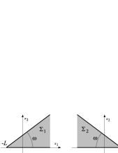
Figure 1: The infinite sectors $\Sigma_{1}$ and $\Sigma_{2}$.

Let us describe our result. Let $\omega\in(0,\pi)$ and $L>0$. Denote by $\Omega_{L}$ the intersection of the two infinite sectors $\Sigma_{1}$ and $\Sigma_{2}$,

$$\Sigma_{1} :=\Big{\{}(x_{1},x_{2}):\arg\big{(}(x_{1}+L)+ix_{2}\big{)}\in(0,\omega)\Big{\}},$$

$$\Sigma_{2} :=\big{\{}(x_{1},x_{2}):(-x_{1},x_{2})\in\Sigma_{1}\big{\}},$$

see Fig. 1. Clearly, for $\omega\geq\pi/2$ the set $\Omega_{L}$ is an infinite biangle whose vertices are the points $A_{1}=(-L,0)$ and $A_{2}=(L,0)$, while for $\omega<\pi/2$ we obtain the interior of the triangle whose vertices are the above points $A_{1}$ and $A_{2}$ and the point $A_{3}=(0,L\tan\omega)$, see Figure 2. Let us fix some $\beta>0$. The associated Robin Laplacian

$$H_{L}:=H(\Omega_{L},\beta)$$

is a self-adjoint operator in $L^{2}(\Omega_{L};\mathbb{R})$, see Subsection 2.3 for the rigorous definition. Elementary considerations show that if $\omega<\pi/2$, then $H_{L}$ has a compact resolvent, and the spectrum consists of eigenvalues $E_{1}(L)<E_{2}(L)\leq\dots$. As usually, each eigenvalue may appear several times according to its multiplicity. For $\omega\geq\pi/2$ one has

$$\operatorname{spec}_{\text{ess}}H_{L}=[-\beta^{2},+\infty)\,,$$

so the discrete spectrum consists of eigenvalues $E_{1}(L)<E_{2}(L)\leq\dots<-\beta^{2}\,$.

Our main result is as follows:

Theorem 1.1.

Assume that either $\omega\in\big{(}0,\frac{\pi}{3}\big{)}$ or $\omega\in\big{[}\frac{\pi}{2},\pi\big{)}$. Then, the two lowest eigenvalues satisfy, as $L\to+\infty$,

$$E_{1}(L) =-\dfrac{2\beta^{2}}{1-\cos\omega}$$

$$\quad-4\beta^{2}\dfrac{1+\cos\omega}{(1-\cos\omega)^{2}}\exp\Big{(}-2\beta\dfrac{1+\cos\omega}{\sin\omega}L\Big{)}+O\bigg{(}L^{2}\exp\Big{(}-(2+\delta)\beta\dfrac{1+\cos\omega}{\sin\omega}L\Big{)}\bigg{)},$$

$$E_{2}(L) =-\dfrac{2\beta^{2}}{1-\cos\omega}$$

$$\quad+4\beta^{2}\dfrac{1+\cos\omega}{(1-\cos\omega)^{2}}\exp\Big{(}-2\beta\dfrac{1+\cos\omega}{\sin\omega}L\Big{)}+O\bigg{(}L^{2}\exp\Big{(}-(2+\delta)\beta\dfrac{1+\cos\omega}{\sin\omega}L\Big{)}\bigg{)},$$

where $\delta=2\big{(}(\cos\omega)^{-1}-1\big{)}$ for $\theta<\pi/3$ and $\delta=2$ for $\omega\geq\pi/2\,$. In particular,

$$E_{2}(L)-E_{1}(L)=8\beta^{2}\dfrac{1+\cos\omega}{(1-\cos\omega)^{2}}\exp\Big{(}-2\beta\dfrac{1+\cos\omega}{\sin\omega}L\Big{)}\\ +O\bigg{(}L^{2}\exp\Big{(}-(2+\delta)\beta\dfrac{1+\cos\omega}{\sin\omega}L\Big{)}\bigg{)}.$$

Our proof is in the spirit of the scheme developed by Helffer and Sjöstrand for the semiclassical analysis of the multiple well problem [HS1, H]. In Section 2 we introduce the necessary tools and establish some basic properties of the Robin Laplacians in polygons. Section 3 is devoted to the proof of Theorem 1.1. In Section 4 we discuss possible generalizations and variants. In Appendix A we study the one-dimensional Robin problem which is used to obtain a more precise result for the case $\omega=\frac{\pi}{2}$.

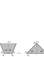
Figure 2: The domain $\Omega_{L}$ for $\omega\geq\dfrac{\pi}{2}$ (left) and $\omega<\dfrac{\pi}{2}$ (right).

Acknowledgments. The research was partially supported by ANR NOSEVOL and GDR Dynamique quantique. Bernard Helffer is also associated with the laboratoire Jean Leray at the university of Nantes.

2 Preliminaries

2.1 Basic tools in functional analysis

Recall the max-min principle for the self-adjoint operators.

Proposition 2.1.

Let $A$ be a lower semibounded self-adjoint operator in a Hilbert space $\mathcal{H}$, and let $E:=\inf\operatorname{spec}_{\mathrm{ess}}A$. For $n\in\mathbb{N}$ consider the quantities

$$E_{n}:=\sup_{\psi_{1},\dots,\psi_{n-1}\in\mathcal{H}}\inf_{\begin{subarray}{c}u\in D(A),\,u\neq 0\\ u\perp\psi_{1},\dots,\psi_{n-1}\end{subarray}}\dfrac{\langle u,Au\rangle}{\langle u,u\rangle}.$$

If $E_{n}<E$, then $E_{n}$ is the $n$th eigenvalue of $A$ (if numbered in the non-decreasing order and counted with multiplicities). Furthermore, one obtains an equivalent definition of $E_{n}$ by setting

$$E_{n}:=\sup_{\psi_{1},\dots,\psi_{n-1}\in\mathcal{H}}\inf_{\begin{subarray}{c}u\in Q(A),\,u\neq 0\\ u\perp\psi_{1},\dots,\psi_{n-1}\end{subarray}}\dfrac{a(u,u)}{\langle u,u\rangle},$$

where $Q(A)$ is the form domain of $A$ and $a$ is the associated bilinear form.

Let $\mathcal{H}$ be a Hilbert space. For a closed subspace $L$ of $\mathcal{H}$, we denote by $P_{L}$ the orthogonal projector on $L$ in $\mathcal{H}$. For an ordered pair $(E,F)$ of closed subspaces $E$ and $F$ of $\mathcal{H}$ we define

$$d(E,F)=\|P_{E}-P_{F}P_{E}\|\equiv\|P_{E}-P_{E}P_{F}\|.$$

The following proposition summarizes some essential properties, cf. [HS1, Lemma 1.3 and Proposition 1.4]:

Proposition 2.2.

The distance between subspaces has the following properties:

1. $d(E,F)=0$ if and only if $E\subset F$,

2. $d(E,G)\leq d(E,F)+d(E,G)$ for any closed subspace $G$ of $\mathcal{H}$,

3. if $d(E,F)<1$, then then the map $E\ni f\mapsto P_{F}f\in F$ is injective, and the map $F\ni f\mapsto P_{E}f\in E$ has a continuous right inverse,

4. If $d(E,F)<1$ and $d(F,E)<1$, then $d(E,F)=d(F,E)$, the map $F\ni f\mapsto P_{E}f\in E$ is bijective, and its inverse is continuous.

The following proposition can be used to estimate $d(E,F)$, see e.g. [HS1, Proposition 3.5].

Proposition 2.3.

Let $A$ be a self-adjoint operator in $\mathcal{H}$, $I\subset\mathbb{R}$ be a compact interval, $\psi_{1},\dots,\psi_{n}\in D(A)$ be linearly independent, and $\mu_{1},\dots,\mu_{n}\in\mathbb{R}\,$. Denote:

$$\varepsilon :=\max_{j\in\{1,\dots,n\}}\big{\|}(A-\mu_{j})\psi_{j}\big{\|}\,,$$

$$a :=\frac{1}{2}\operatorname{dist}\big{(}I,(\operatorname{spec}A)\setminus I\big{)}\,,$$

$$\Lambda :=\text{ the smallest eigenvalue of the Gramian matrix }\big{(}\langle\psi_{j},\psi_{k}\rangle\big{)}\,.$$

Let $E$ be the subspace spanned by $\psi_{1},\dots,\psi_{n}$ and $F$ be the spectral subspace associated with $A$ and $I$. If $a>0\,$, then

$$d(E,F)\leq\dfrac{1}{a}\sqrt{\dfrac{n}{\Lambda}}\,\varepsilon\,.$$ (2)

2.2 Robin Laplacians in infinite sectors

For $\alpha\in(0,\pi)$, we define

$$S_{\alpha}:=\big{\{}(x_{1},x_{2})\in\mathbb{R}^{2}:\quad\big{|}\arg(x_{1}+ix_{2})\big{|}<\alpha\big{\}}$$

and consider the associated Robin Laplacian and the bottom of its spectrum:

$$H_{\alpha}=H(S_{\alpha},\beta)\,,\quad E_{\alpha}:=\inf\operatorname{spec}H_{\alpha}\,.$$

The following result is essentially contained in [LP]:

Proposition 2.4.

The operator $H_{\alpha}$ has the following properties:

• If $\alpha<\frac{\pi}{2}$, then

  $$E_{\alpha}=-\dfrac{\beta^{2}}{\sin^{2}\alpha},$$ (3)

  and this point is a simple isolated eigenvalue of $\operatorname{spec}H_{\alpha}$ with the associated normalized eigenfunction

  $$U_{\alpha}(x_{1},x_{2})=\beta\sqrt{\dfrac{2\cos\alpha}{\sin^{3}\alpha}}\exp\Big{(}-\dfrac{\beta}{\sin\alpha}x_{1}\Big{)}\,.$$ (4)

• If $\alpha\geq\frac{\pi}{2}$, then $E_{\alpha}=-\beta^{2}$ and $\operatorname{spec}H_{\alpha}=[E_{\alpha},+\infty)\,$.

In what follows we will use another associated quantity,

$$\Lambda_{\alpha}:=\inf(\operatorname{spec}H_{\alpha})\setminus\{E_{\alpha}\}.$$ (5)

In view of Proposition 2.4 we have:

• if $\alpha<\frac{\pi}{2}$, then $\Lambda_{\alpha}>E_{\alpha}$. In this case, if one denotes by $P_{\alpha}$ the orthogonal projection in $L^{2}(S_{\alpha})$ onto the subspace spanned by $U_{\alpha}$, then the spectral theorem implies

  $$\langle u,H_{\alpha}u\rangle\geq\Lambda_{\alpha}\|u\|^{2}+(E_{\alpha}-\Lambda_{\alpha})\big{\langle}u,P_{\alpha}u\big{\rangle}\text{ for all }u\in D(H_{\alpha})\,,$$ (6)

• if $\alpha\geq\frac{\pi}{2}$, then $\Lambda_{\alpha}=E_{\alpha}\,$.

2.3 Robin Laplacians in convex polygons

In this subsection, let $\Omega_{1}\subset\mathbb{R}^{2}$ be a convex polygonal domain, i.e. is the intersection of finitely many half-planes. Assume that $\Omega_{1}$ has $N$ vertices $B_{1},\dots,B_{N}$, and the corner opening at $B_{j}$ will be denoted by $2\alpha_{j}$. We assume that all vertices are non-trivial, which means, due to the convexity, that $\alpha_{j}\in(0,\frac{\pi}{2})$ for all $j$. Define

$$\alpha:=\min_{j}\alpha_{j}\,.$$

Furthermore, we set $\Omega_{L}:=L\Omega_{1}$ for some $L>0$ and denote by $A_{j}:=LB_{j}$ the vertices of $\Omega_{L}$. We omit sometimes the reference to $L$ and write more simply $\Omega\,$. Finally, let us pick some $\beta>0$ and consider the associated Robin Laplacian $H:=H(\Omega,\beta)$. Strictly speaking, $H$ is the operator associated with the bilinear form

$$h_{\Omega,\beta}(u,u)=\iint_{\Omega}|\nabla u|^{2}\,dx-\beta\int_{\partial\Omega}|u|^{2}\,ds\,,\quad u\in H^{1}(\Omega)\,,$$

where $ds$ means the integration with respect to the length parameter. Using the standard methods we have

$$\inf\operatorname{spec}_{\text{ess}}H\geq-\beta^{2}\,.$$

The following proposition is a particular case of a more general result proved in [LP]:

Proposition 2.5.

$\lim_{L\to+\infty}\inf\operatorname{spec}H=-\dfrac{\beta^{2}}{\sin^{2}\alpha}\equiv E_{\alpha}$.

To describe the domain of $H$, let us recall first the Green-Riemann formula, which states that, for $f\in H^{1}(\Omega)$ and $g\in H^{2}(\Omega)$,

$$\int_{\partial\Omega}f\,\dfrac{\partial g}{\partial n}\,ds=\iint_{\Omega}\Big{(}f\Delta g+\nabla f\cdot\nabla g\Big{)}\,dx\,,$$ (7)

where $n$ is the outward unit normal.

Proposition 2.6.

There holds

$$D(H)=\big{\{}u\in H^{2}(\Omega):\dfrac{\partial u}{\partial n}=\beta u\text{ at }\partial\Omega\big{\}}$$ (8)

and $Hu=-\Delta u$ for all $u\in D(H)$.

Proof.

The claim follows from the general scheme developped for boundary value problems in non-smooth domains [G]. We just explain briefly how this scheme appplies to the Robin boundary condition. We note first that the associated form $h_{\Omega,\beta}$ is semibounded from below and closed due to the standard Sobolev embedding theorems. We note then that for any $u\in D(H)$ one has $Hu=-\Delta u$ in $\mathcal{D}^{\prime}(\Omega)$. Furthermore, if $\widetilde{D}$ is the set on the right-hand side of (8), then it easily follows from (7) that $\widetilde{D}\subset D(H)$. It follows also that for $f\in H^{2}(\Omega)$ the inclusion $f\in D(H)$ is equivalent to the equality $\partial f/\partial n=\beta f$ on $\partial\Omega\,$. In view of these observations, it is sufficient to show that $D(H)\subset H^{2}(\Omega)$.

Take any $f\in D(H)\subset H^{1}(\Omega)$ and let $g:=Hf\in L^{2}(\Omega)$. All corners at the boundary of $\Omega$ are smaller than $\pi$, and the trace of $f$ on $\partial\Omega$ is in $H^{\frac{1}{2}}(\partial\Omega)$, which means that there exists a solution $u\in H^{2}(\Omega)$ for the boundary value problem:

$$-\Delta u=g\text{ in }\Omega,\,\dfrac{\partial u}{\partial n}=\beta f\text{ on }\partial\Omega\,,$$

see [G, Section 2.4] (we are in the case where no singular solutions are present). On the other hand, $f$ is a variational solution of the preceding problem. This means that the function $v:=f-u\in H^{1}(\Omega)$ becomes a variational solution to

$$-\Delta v=0\text{ in }\mathcal{D}^{\prime}(\Omega),\,\dfrac{\partial v}{\partial n}=0\text{ on }\partial\Omega\,.$$

Again according to [G, Section 2.4] we conclude that the only possible solution is constant, which means that $f=u+v\in H^{2}(\Omega)$. ∎

Now let us obtain some (Agmon-type) decay estimates of the eigenfunctions of $H$ corresponding to the lowest eigenvalues as $L\to+\infty$. Let us start with a technical identity.

Lemma 2.7.

Let $u\in H^{2}(\Omega)$ be real-valued and satisfy the Robin boundary condition $\partial u/\partial n=\beta u$ at $\partial\Omega$. Furthermore, let $\Phi:\Omega\to\mathbb{R}$ be such that $\Phi,\nabla\Phi\in L^{\infty}(\Omega)$, then

$$\iint_{\Omega}\big{|}\nabla(e^{\Phi}u)\big{|}^{2}dx-\beta\int_{\partial\Omega}e^{2\Phi}u^{2}ds=\iint_{\Omega}e^{2\Phi}u(-\Delta u)dx+\iint_{\Omega}|\nabla\Phi|^{2}e^{2\Phi}u^{2}dx.$$

Proof.

We just consider the case $\Phi\in C^{2}(\overline{\Omega})$, then one can pass to the general case using the standard regularization procedure. We have

$$\big{|}\nabla(e^{\Phi}u)\big{|}^{2} =\Big{(}\dfrac{\partial}{\partial x_{1}}(e^{\Phi}u)\Big{)}^{2}+\Big{(}\dfrac{\partial}{\partial x_{2}}(e^{\Phi}u)\Big{)}^{2}$$

$$=\Big{(}\dfrac{\partial\Phi}{\partial x_{1}}e^{\Phi}u+e^{\Phi}\dfrac{\partial u}{\partial x_{1}}\Big{)}^{2}+\Big{(}\dfrac{\partial\Phi}{\partial x_{2}}e^{\Phi}u+e^{\Phi}\dfrac{\partial u}{\partial x_{2}}\Big{)}^{2}$$

$$=|\nabla\Phi|^{2}e^{2\Phi}u^{2}+2e^{\Phi}u\nabla\Phi\cdot\nabla u+e^{2\Phi}|\nabla u|^{2}$$

$$=|\nabla\Phi|^{2}e^{2\Phi}u^{2}+\nabla(e^{2\Phi}u)\cdot\nabla u\,.$$

Integrating this equality in $\Omega$, we arrive at

$$\iint_{\Omega}\big{|}\nabla(e^{\Phi}u)\big{|}^{2}dx=\iint_{\Omega}|\nabla\Phi|^{2}e^{2\Phi}u^{2}dx+\iint_{\Omega}\nabla(e^{2\Phi}u)\cdot\nabla udx\\ =\iint_{\Omega}|\nabla\Phi|^{2}e^{2\Phi}u^{2}dx+\int_{\partial\Omega}e^{2\Phi}u\dfrac{\partial u}{\partial n}ds+\iint_{\Omega}e^{2\Phi}u(-\Delta u)dx\\ =\iint_{\Omega}|\nabla\Phi|^{2}e^{2\Phi}u^{2}dx+\beta\int_{\partial\Omega}e^{2\Phi}u^{2}ds+\iint_{\Omega}e^{2\Phi}u(-\Delta u)\,dx\,.$$

∎

Now, let us choose a constant $b>0$ such that all corners of $\Omega$ are contained in the ball of radius $bL$ centered at the origin, and consider the function $\Phi:\Omega\to\mathbb{R}$ defined by

$$\Phi(x):=\beta\min\Big{\{}\min_{j\in\{1,\dots,N\}}\cot\alpha_{j}\cdot|x-A_{j}|,bL\Big{\}}.$$

For a compact $\Omega$ we choose the constant $b$ sufficiently large, so that the exterior minimum can be dropped.

Proposition 2.8.

Let $\lambda=\lambda(L)>0$ be such that

$$\lim_{L\to+\infty}\lambda(L)=0\,.$$

Then, for any $\varepsilon\in(0,1)$ there exists $C_{\varepsilon}>0$ and $L_{\varepsilon}$ such that, if $E=E(L)$ is an eigenvalue of $H$ satisfying

$$E\leq-\,\dfrac{\beta^{2}}{\sin^{2}\alpha}+\lambda\,,$$ (9)

and $u$ is an associated normalized eigenfunction, then

$$\big{\|}e^{(1-\varepsilon)\Phi}u\big{\|}_{H^{1}(\Omega)}\leq C_{\varepsilon}e^{\varepsilon L}\quad\text{for}\quad L\geq L_{\epsilon}\,.$$

Proof.

Let $r>0$. Let us pick a $C^{\infty}$ function $\chi:[0,+\infty)\to[0,1]$ such that $\chi(t)=1$ for $t\leq r$ and $\chi(t)=0$ for $t>2r$, and introduce

$$\widetilde{\chi}_{j}(x)=\chi\Big{(}\dfrac{|x-A_{j}|}{L}\Big{)},\quad j=1,\dots,N\,.$$

We assume that $r$ is sufficiently small, which ensures that the supports of $\widetilde{\chi}_{j}$ are disjoint and that $\Phi(x)=\beta\cot\alpha_{j}\,|x-A_{j}|$ for $x\in\operatorname{supp}\widetilde{\chi}_{j}$. An exact value of $r$ will be chosen later. We also complete by the function

$$\widetilde{\chi}_{0}:=1-\sum_{j=1}^{N}\widetilde{\chi}_{j}\,,$$

and, finally, set

$$\chi_{j}:=\widetilde{\chi}_{j}\Big{/}\sqrt{\sum_{k=0}^{N}\widetilde{\chi}_{k}^{2}},\quad j=0,\dots,N.$$

We observe that we have the equalities $\operatorname{supp}\chi_{j}=\operatorname{supp}\widetilde{\chi}_{j}$, that each $\chi_{j}$ is $C^{\infty}$, and that

$$\sum_{j=0}^{N}\chi_{j}^{2}=1\,.$$

For any $v\in H^{1}(\Omega)$ we also have $\chi_{j}v\in H^{1}(\Omega)$, and by a direct computation one obtains

$$h_{\Omega,\beta}(v,v)=\sum_{j=0}^{N}h_{\Omega,\beta}(\chi_{j}v,\chi_{j}v)-\sum_{j=0}^{N}\big{\|}v\nabla\chi_{j}\big{\|}^{2}\,.$$

By construction of $\chi_{j}$, we one can find a constant $C>0$ independent of $v$ and $L$ with

$$h_{\Omega,\beta}(v,v)\geq\sum_{j=0}^{N}h_{\Omega,\beta}(\chi_{j}v,\chi_{j}v)-\dfrac{C}{L^{2}}\|v\|^{2}\text{ for large }L\,.$$

Now let us denote $\Psi:=(1-\varepsilon)\Phi$. By applying the preceding inequality we obtain

$$I:=\iint_{\Omega}\big{|}\nabla(e^{\Psi}u)\big{|}^{2}dx-\beta\int_{\partial\Omega}|e^{\Psi}u|^{2}ds\geq\delta\iint_{\Omega}\big{|}\nabla(e^{\Psi}u)\big{|}^{2}\,dx\\ +(1-\delta)\bigg{[}\sum_{j=0}^{N}\Big{(}\iint_{\Omega}\big{|}\nabla(\chi_{j}e^{\Psi}u)\big{|}^{2}\,dx-\dfrac{\beta}{1-\delta}\int_{\partial\Omega}\big{|}\chi_{j}e^{\Psi}u\big{|}^{2}\,ds\Big{)}-\dfrac{C}{L^{2}}\iint_{\Omega}|e^{\Psi}u|^{2}\,dx\,,\bigg{]},$$ (10)

where $\delta\in(0,1)$ is a constant which will be chosen later.

Furthermore, considering $\chi_{j}e^{\Psi}u$ as a function from $H^{1}(S_{j})$, where $S_{j}$ is a suitably rotated copy of the sector $S_{\alpha_{j}}$ (see Subsection 2.2) which coincides with $\Omega$ near $A_{j}$, we have, for $j=1,\dots,N$,

$$\iint_{\Omega}\big{|}\nabla(\chi_{j}e^{\Psi}u)\big{|}^{2}dx-\dfrac{\beta}{1-\delta}\int_{\partial\Omega}\big{|}\chi_{j}e^{\Psi}u\big{|}^{2}ds\geq-\dfrac{\beta^{2}}{(1-\delta)^{2}\sin^{2}\alpha_{j}}\iint_{\Omega}|\chi_{j}e^{\Psi}u|^{2}dx.$$

By the preceding constructions, the support of $\chi_{0}$ is of the form $\operatorname{supp}\chi_{0}=L\Omega^{\prime}$ with some $L$-independent $\Omega^{\prime}$. Furthermore, one can construct a smooth domain $D$ with $L\Omega^{\prime}\subset LD\subset\Omega$ and such that $\partial(L\Omega^{\prime})\cap\partial\Omega=\partial(LD)\cap\partial\Omega$. As mentioned in the introduction, the lowest eigenvalue of $H\big{(}LD,\beta/(1-\delta)\big{)}$ for large $L$ converges to $-\beta^{2}/(1-\delta)^{2}$, i.e. for any $v\in H^{1}(LD)$ we have

$$\iint_{LD}\big{|}\nabla v\big{|}^{2}dx-\dfrac{\beta}{1-\delta}\int_{\partial(LD)}|v|^{2}ds\geq-\Big{(}\dfrac{\beta^{2}}{(1-\delta)^{2}}+\varepsilon_{0}\Big{)}\iint_{LD}|v|^{2}dx,$$

where $\varepsilon_{0}:=\varepsilon_{0}(L,\delta)>0$ is such that $\lim_{L\to+\infty}\varepsilon_{0}=0$ for any fixed $\delta\in(0,1)$. By taking $v=\chi_{0}e^{\Psi}u$ we obtain

$$\iint_{\Omega}\big{|}\nabla(\chi_{0}e^{\Psi}u)\big{|}^{2}dx-\dfrac{\beta}{1-\delta}\int_{\partial\Omega}\big{|}\chi_{0}e^{\Psi}u\big{|}^{2}ds\geq-\Big{(}\dfrac{\beta^{2}}{(1-\delta)^{2}}+\varepsilon_{0}\Big{)}\iint_{\Omega}|\chi_{0}e^{\Psi}u|^{2}dx.$$

Putting the preceding estimates together we arrive at

$$I\geq\delta\iint_{\Omega}\big{|}\nabla(e^{\Psi}u)\big{|}^{2}dx-\Big{(}\dfrac{\beta^{2}}{1-\delta}+\dfrac{(1-\delta)C}{L^{2}}+\varepsilon_{1}\Big{)}\iint_{\Omega}|\chi_{0}e^{\Psi}u|^{2}dx\\ -\sum_{j=1}^{N}\Big{(}\dfrac{\beta^{2}}{(1-\delta)\sin^{2}\alpha_{j}}+\dfrac{(1-\delta)C}{L^{2}}\Big{)}\iint_{\Omega}|\chi_{j}e^{\Psi}u|^{2}dx$$ (11)

with $\varepsilon_{1}:=(1-\delta)\varepsilon_{0}$. On the other hand, due to Lemma 2.7 we have

$$I=\iint_{\Omega}e^{2\Psi}u(-\Delta u)dx+\iint_{\Omega}|\nabla\Psi|^{2}e^{2\Psi}u^{2}\,dx\\ =E\iint_{\Omega}e^{2\Psi}u^{2}dx+\iint_{\Omega}|\nabla\Psi|^{2}e^{2\Psi}u^{2}\,dx=\sum_{j=0}^{N}\iint_{\Omega}\big{(}E+|\nabla\Psi|^{2}\big{)}|\chi_{j}e^{\Psi}u|^{2}\,dx\,.$$ (12)

We estimate as follows:

$$\big{|}\nabla\Psi(x)\big{|}\leq(1-\varepsilon)^{2}\beta^{2}\cot\alpha\equiv(1-\varepsilon)^{2}\beta^{2}\Big{(}\dfrac{1}{\sin^{2}\alpha}-1\Big{)},\quad x\in\operatorname{supp}\chi_{0}\,,$$

$$\big{|}\nabla\Psi(x)\big{|}\leq(1-\varepsilon)^{2}\beta^{2}\cot\alpha_{j}\equiv(1-\varepsilon)^{2}\beta^{2}\Big{(}\dfrac{1}{\sin^{2}\alpha_{j}}-1\Big{)},\quad x\in\operatorname{supp}\chi_{j}\,,\quad j=1,\dots,N\,.$$

Substituting these two inequalities into (12) and using (9) we arrive at

$$I \leq\bigg{(}-\dfrac{\beta^{2}}{\sin^{2}\alpha}+\lambda+(1-\varepsilon)^{2}\beta^{2}\Big{(}\dfrac{1}{\sin^{2}\alpha}-1\Big{)}\bigg{)}\iint_{\Omega}|\chi_{0}e^{\Psi}u|^{2}dx$$

$$\quad+\sum_{j=1}^{N}\bigg{(}-\dfrac{\beta^{2}}{\sin^{2}\alpha}+\lambda+(1-\varepsilon)^{2}\beta^{2}\Big{(}\dfrac{1}{\sin^{2}\alpha_{j}}-1\Big{)}\bigg{)}\iint_{\Omega}|\chi_{j}e^{\Psi}u|^{2}\,dx\,.$$

Combining with (11) we have:

$$\delta\iint_{\Omega}\big{|}\nabla(e^{\Psi}u)\big{|}^{2}\,dx+C_{0}\iint_{\Omega}|\chi_{0}e^{\Psi}u|^{2}\,dx\leq\sum_{j=1}^{N}C_{j}|\chi_{j}e^{\Psi}u|^{2}\,dx\,,$$

where

$$\begin{aligned} C_{0}&:=(2\varepsilon-\varepsilon^{2})\Big{(}\dfrac{1}{\sin^{2}\alpha}-1\Big{)}\,\beta^{2}-\dfrac{\delta}{1-\delta}\,\beta^{2}-\dfrac{(1-\delta)C}{L^{2}}-\varepsilon_{1}-\lambda\,,\\ C_{j}&:=-\dfrac{\beta^{2}}{\sin^{2}\alpha}+(1-\varepsilon)^{2}\Big{(}\dfrac{1}{\sin^{2}\alpha_{j}}-1\Big{)}\beta^{2}+\dfrac{\beta^{2}}{(1-\delta)\sin^{2}\alpha_{j}}+\dfrac{(1-\delta)C}{L^{2}}+\lambda\,,\,j=1,\dots,N\,.\end{aligned}$$

As $\varepsilon>0$ is a fixed positive number and both $\varepsilon_{1}$ and $\lambda$ tend to $0$ as $L\to+\infty\,$, we can find $m_{\varepsilon}>0$, $\delta>0$ and $L_{0}>0$ such that $C_{0}\geq m_{\varepsilon}$ for all $L>L_{0}\,$. At the same time, for the same $\delta$ and $L$ we may estimate $C_{j}\leq M_{\varepsilon}\,$, $j=1,\dots,N\,$, which gives

$$\iint_{\Omega}\big{|}\nabla(e^{\Psi}u)\big{|}^{2}\,dx+\iint_{\Omega}|\chi_{0}e^{\Psi}u|^{2}\,dx\leq C_{\varepsilon}\sum_{j=1}^{N}|\chi_{j}e^{\Psi}u|^{2}\,dx\,,\quad C_{\varepsilon}:=\dfrac{M_{\varepsilon}}{\delta}+\dfrac{M_{\varepsilon}}{m_{\varepsilon}}\,.$$

Now we get the estimate

$$\|e^{(1-\varepsilon)\Phi}u\|^{2}_{H^{1}(\Omega)}=\|e^{\Psi}u\|^{2}_{H^{1}(\Omega)}=\iint_{\Omega}\big{|}\nabla(e^{\Psi}u)\big{|}^{2}\,dx+\iint_{\Omega}|e^{\Psi}u|^{2}\,dx\\ =\iint_{\Omega}\big{|}\nabla(e^{\Psi}u)\big{|}^{2}\,dx+\iint_{\Omega}|\chi_{0}e^{\Psi}u|^{2}\,dx+\sum_{j=1}^{N}|\chi_{j}e^{\Psi}u|^{2}\,dx\leq(1+C_{\varepsilon})\sum_{j=1}^{N}|\chi_{j}e^{\Psi}u|^{2}\,dx\\ \leq(1+C_{\varepsilon})\exp\Big{[}(1-\varepsilon)\max_{j\in\{1,\dots,N\}}\sup_{x\in\operatorname{supp}\chi_{j}}\Phi(x)\Big{]}\sum_{j=1}^{N}\iint_{\Omega}|\chi_{j}u|^{2}\,dx\,.$$

We have

$$\sum_{j=1}^{N}\iint_{\Omega}|\chi_{j}u|^{2}\,dx\leq\sum_{j=0}^{N}\iint_{\Omega}|\chi_{j}u|^{2}\,dx=\iint_{\Omega}|u|^{2}\,dx=1\,,$$

and

$$\max_{j\in\{1,\dots,N\}}\sup_{x\in\operatorname{supp}\chi_{j}}\Phi(x)\leq 2r\beta(\cot\alpha)L\,.$$

Therefore, by taking $r<\varepsilon/(2t\beta\cot\alpha)\,$, we get the conclusion. ∎

3 The lowest eigenvalues of $H_{L}$

3.1 Notation

In this section we study in greater detail the lowest eigenvalues of the operator $H_{L}$. We collect first some notation and conventions used below. Note that all the assertions of Section 2 are applicable to $H_{L}$ as well. Throughout the section we will write

$$\alpha:=\dfrac{\omega}{2}\quad\mbox{ and }\quad\Omega:=\Omega_{L}\,.$$

Furthermore, we introduce the following transformations of $\mathbb{R}^{2}\,$:

$$R_{1}(x_{1},x_{2})=\begin{pmatrix}\cos\alpha&\sin\alpha\\ -\sin\alpha&\cos\alpha\end{pmatrix}\begin{pmatrix}x_{1}+L\\ x_{2}\end{pmatrix},\quad R_{2}(x_{1},x_{2})=\begin{pmatrix}\cos\alpha&\sin\alpha\\ \sin\alpha&-\cos\alpha\end{pmatrix}\begin{pmatrix}L-x_{1}\\ x_{2}\end{pmatrix}.$$

The geometric meaning of $R_{j}$ is clear from the equalities $R_{j}(\Sigma_{j})=S_{\alpha}$, $j=1,2$, and we consider the associated rotated eigenfunctions

$$U_{j}(x):=U_{\alpha}(R_{j}x)\,,\,j=1,2\,.$$

Recall that $S_{\alpha}$ and $U_{\alpha}$ are defined in Subsection 2.2, so we have

$$U_{1}(x_{1},x_{2}) =\beta\sqrt{\dfrac{2\cos\alpha}{\sin^{3}\alpha}}\,e^{-\beta(x_{1}+L)\cot\alpha-\beta x_{2}},$$ (13)

$$U_{2}(x_{1},x_{2}) =\beta\sqrt{\dfrac{2\cos\alpha}{\sin^{3}\alpha}}\,e^{-\beta(L-x_{1})\cot\alpha-\beta x_{2}}.$$

We also recall the notation

$$E_{\alpha}:=-\beta^{2}/\sin^{2}\alpha\,.$$

Furthermore, for $j=1,2$ we denote by $M_{j}$ the Robin Laplacian in $\Sigma_{j}$,

$$M_{j}:=H(\Sigma_{j},\beta)\,.$$

3.2 A rough eigenvalue estimate

Let us obtain some rough information on the behavior of the eigenvalues of $H_{L}$ as $L$ tends to $+\infty$. Assuming that $H_{L}$ has at least $n-1$ eigenvalues below the essential spectrum, we denote

$$\widetilde{E}_{n}(L):=\inf(\operatorname{spec}H_{L})\setminus\big{\{}E_{1}(L),\dots,E_{n-1}(L)\big{\}}\,,$$

Lemma 3.1.

Let $\omega\in\big{(}0,\frac{\pi}{3}\big{)}\mathbin{\cup}\big{[}\frac{\pi}{2},\pi\big{)}$, then for sufficiently large $L$ the operator $H_{L}$ has at least two eigenvalues below the essential spectrum, and one has

$$\lim_{L\to+\infty}E_{j}(L)=E_{\alpha},\quad j=1,2\,,$$ (14)

$$\liminf_{L\to+\infty}\widetilde{E}_{3}(L)>E_{\alpha}\,.$$ (15)

Proof.

For $\delta>0$, let us pick a $C^{\infty}$ function $\chi:\mathbb{R}_{+}\to[0,1]$ such that $\chi(t)=1$ for $t\leq\delta$ and $\chi(t)=0$ for $t>2\delta\,$. Introduce the functions

$$\widetilde{\chi}_{j}(x)=\chi\Big{(}\dfrac{|x-A_{j}|}{L}\Big{)},\quad j=1,2\,.$$

We assume that $\delta$ is sufficiently small, which ensures that the supports of $\widetilde{\chi}_{1}$ and $\widetilde{\chi}_{2}$ do not intersect, and consider the functions

$$v_{j}:=\widetilde{\chi}_{j}U_{j}\,,\quad j=1,2.$$

By a simple computation, as $L\to+\infty$ we have

$$\iint_{\Omega}v_{j}v_{k}\,dx=\delta_{jk}+o(1),\quad\iint_{\Omega}\nabla v_{j}\cdot\nabla v_{k}\,dx-\beta\int_{\partial\Omega}v_{j}v_{k}\,ds=E_{\alpha}\delta_{jk}+o(1)\,,\quad j,k=1,2.$$

It follows that

$$\sup_{0\not\equiv v\in\operatorname{Span}(v_{1},v_{2})}\dfrac{h_{\Omega,\beta}(v,v)}{\langle v,v\rangle}\leq E_{\alpha}+o(1)<-\beta^{2}\equiv\inf\operatorname{spec}_{\text{ess}}H_{L}\,,$$

the last inequality being true for $L$ large enough.

On the other hand, the functions $v_{1}$ and $v_{2}$ are linearly independent. It follows that for any $\psi\in L^{2}(\Omega)$ one can find a non-trivial linear combination $v\in\operatorname{Span}(v_{1},v_{2})$ which is orthogonal to $\psi$. Due to the previous estimate and Proposition 2.1 we obtain then

$$E_{2}(L)\leq E_{\alpha}+o(1)\,.$$

Combining with $E_{2}(L)\geq E_{1}(L)\,$, and with the result of Proposition 2.5, this gives (14).

Let us now prove (15). Let us introduce

$$\widetilde{\chi}_{0}:=1-\widetilde{\chi}_{1}-\widetilde{\chi}_{2}$$

and set

$$\chi_{j}:=\widetilde{\chi}_{j}\Big{/}\sqrt{\sum_{k=0}^{2}\widetilde{\chi}_{k}^{2}},\quad j=0,1,2.$$

By a direct computation, for any $u\in H^{1}(\Omega)$ we have

$$h_{\Omega,\beta}(u,u)=\sum_{j=0}^{2}h_{\Omega,\beta}(\chi_{j}u,\chi_{j}u)-\sum_{j=0}^{2}\big{\|}u\nabla\chi_{j}\big{\|}^{2},$$

and by the construction of $\chi_{j}$, we can find $L_{0}>0$ and $C>0$ such that for all $u$ and $L\geq L_{0}$

$$h_{\Omega,\beta}(u,u)\geq\sum_{j=0}^{2}h_{\Omega,\beta}(\chi_{j}u)-\dfrac{C}{L^{2}}\|u\|^{2}\,.$$

Furthermore, we have $\chi_{j}u\in H^{1}(\Sigma_{j})\,$, $j=1,2\,$. Consider the orthogonal projections $\Pi_{j}:=\langle U_{j},\cdot\rangle U_{j}$ in $L^{2}(\Sigma_{j})\,$. By applying the inequality (6) we obtain

$$h_{\Omega,\beta}(\chi_{j}u,\chi_{j}u)\geq(E_{\alpha}-\Lambda_{\alpha})\|\Pi_{j}\chi_{j}u\|^{2}_{L^{2}(\Sigma_{j})}+\Lambda_{\alpha}\|\chi_{j}u\|^{2}_{L^{2}(\Sigma_{j})},\quad j=1,2\,.$$

The norms in $L^{2}(\Sigma_{j})$ can be replaced back by the norms in $L^{2}(\Omega)$, and we infer

$$h_{\Omega,\beta}(u,u)\geq\langle u,\Pi u\rangle+\Lambda_{\alpha}\big{(}\|\chi_{1}u\|^{2}+\|\chi_{2}u\|^{2}\big{)}+h_{\Omega,\beta}(\chi_{0}u,\chi_{0}u)-\dfrac{C}{L^{2}}\|u\big{\|}^{2}\,,$$

where $\Pi:=(E_{\alpha}-\Lambda_{\alpha})\big{(}\chi_{1}\Pi_{1}\chi_{1}+\chi_{2}\Pi_{2}\chi_{2}\big{)}$ is an operator whose range is at most two-dimensional.

To estimate the term with $\chi_{0}$, we proceed as in the proof of Proposition 2.8. By the preceding constructions, the support of $\chi_{0}$ has the form $\operatorname{supp}\chi_{0}=L\Omega^{\prime}$ with some $L$-independent $\Omega^{\prime}$. Furthermore, one can construct a convex polygonal domain $D$ with $L\Omega^{\prime}\subset LD\subset\Omega$ such that $\partial(L\Omega^{\prime})\cap\partial\Omega=\partial(LD)\cap\partial\Omega$ and that the minimal corner $\theta$ at the boundary of $D$ is strictly larger than $\omega$. By Proposition 2.5 for any $A<E_{\theta/2}$ and any $v\in H^{1}(LD)$ we have, as $L$ is sufficiently large,

$$h_{LD,\beta}(v,v)\geq A\|v\|^{2}_{L^{2}(LD)}.$$

As $E_{\theta/2}>E_{\omega/2}\equiv E_{\alpha}$, we may assume that $A>E_{\alpha}$. Using the last equality with $v=\chi_{0}u$ we obtain, for large $L$,

$$h_{\Omega,\beta}(\chi_{0}u,\chi_{0}u)\geq A\|\chi_{0}u\|^{2}\,.$$

Putting all together and noting that $\|\chi_{0}u\|^{2}+\|\chi_{1}u\|^{2}+\|\chi_{2}u\|^{2}=\|u\|^{2}$ we obtain, for sufficiently large $L$,

$$h_{\Omega,\beta}(u,u)\geq\langle u,\Pi u\rangle+\Big{(}E-\dfrac{C}{L^{2}}\Big{)}\|u\big{\|}^{2},\quad E=\min(A,\Lambda_{\alpha})>E_{\alpha}\,.$$

Now take two vectors $\psi_{1}$ and $\psi_{2}$ spanning the range of $\Pi\,$. For any non-zero $u\in H^{1}(\Omega)$ which is orthogonal to $\psi_{1}$ and $\psi_{2}$ we have

$$\dfrac{h_{\Omega,\beta}(u,u)}{\langle u,u\rangle}\geq E-\dfrac{C}{L^{2}}\,,$$

which gives the announced inequality (15) by the max-min principle. ∎

The following assertion summarizes the preceding considerations:

Proposition 3.2.

Let $\omega\in\big{(}0,\frac{\pi}{3}\big{)}\mathbin{\cup}\big{[}\frac{\pi}{2},\pi\big{)}$, then there exists $\delta>0$ and $L_{0}$ such that for $L\geq L_{0}$ the spectrum of $H_{L}$ in $(E_{\alpha}-\delta,E_{\alpha}+\delta)$ consists of exactly two eigenvalues $E_{1}(L)$ and $E_{2}(L)$, both converging to $E_{\alpha}$ as $L\to+\infty$.

Remark 3.3.

Indeed, one can prove an analog of Lemma 3.1 for the remaining ranges of $\omega$ in a similar way, and one has:

$$\lim_{L\to+\infty}E_{1}(L)=E_{\alpha}\quad\text{and}\quad\liminf_{L\to+\infty}\widetilde{E}_{2}(L)>E_{\alpha}\quad\text{for }\omega\in\Big{(}\dfrac{\pi}{3},\dfrac{\pi}{2}\Big{)},$$

$$\lim_{L\to+\infty}E_{j}(L)=E_{\alpha},\quad j=1,2,3,\quad\text{and}\quad\liminf_{L\to+\infty}\widetilde{E}_{4}(L)>E_{\alpha}\text{ for }\omega=\dfrac{\pi}{3},$$ (16)

and Proposition 3.2 should be suitably reformulated. We remark that the case $\omega=\pi/3$, i.e. the equilateral triangle, was already studied in [McC, Section 7], where it was found that after a suitable transformation one may separate the variables, and the calculation of the eigenvalues reduces to solving a certain non-linear system, which admits a rather direct analysis. In particular, the second inequality in (16) holds in the stronger form $\lim_{L\to+\infty}\widetilde{E}_{4}(L)=-\beta^{2}$.

For the rest of the section, we assume that

$$\omega\in\Big{(}0,\dfrac{\pi}{3}\Big{)}\mathbin{\cup}\Big{[}\dfrac{\pi}{2},\pi\Big{)}.$$

3.3 Cut-off functions

We are going to introduce a family of cut-off functions adapted to the geometry of the sector $S_{\alpha}$ (see Subsection 2.2). Note that our assumptions imply $\alpha<\frac{\pi}{2}$. Pick a function $\chi:\mathbb{R}\to[0,1]$ such that

$$\chi\in C^{\infty}(\mathbb{R}),\quad\chi(t)=1\text{ for }t\leq-1,\quad\chi(t)=0\text{ for }t\geq 0\,,$$ (17)

and for $\ell>0$ we set

$$\varphi_{\alpha,\ell}(x_{1},x_{2})=\chi(x_{1}-\ell\cos\alpha)\chi\big{(}|x|-(\ell-1)\big{)}\,.$$ (18)

This function has the following properties for large $\ell$, see Figure 3:

$$\begin{gathered}\varphi_{\alpha,\ell}\in C^{\infty}(\overline{S}_{\alpha})\,,\\ \varphi_{\alpha,\ell}(x)\in[0,1]\text{ for all }x\in S_{\alpha}\,,\\ \varphi_{\alpha,\ell}(x)=1\text{ for }x=(x_{1},x_{2})\in\{x_{1}\leq\ell\cos\alpha-2\}\cap S_{\alpha}\,,\\[3.0pt] \varphi_{\alpha,\ell}(x)=0\text{ for }x=(x_{1},x_{2})\notin\{x_{1}\leq\ell\}\cap S_{\alpha}\,,\\ \dfrac{\partial\varphi_{\alpha,\ell}}{\partial n}=0\text{ at }\partial S_{\alpha}\,,\\ \text{$\sum_{|\nu|\leq 2}\|D^{\nu}\varphi_{\alpha,\ell}\|_{\infty}\leq c$ for some $c>0$ independent of $\ell\,$.}\end{gathered}$$ (19)

The slightly involved construction of $\varphi_{\alpha,\ell}$ guarantees that for any function $f\in H^{2}(S_{\alpha})$ with $\partial f/\partial n=\beta f$ at the boundary the product $\varphi_{\alpha,\ell}f$ still satisfies the same boundary condition.

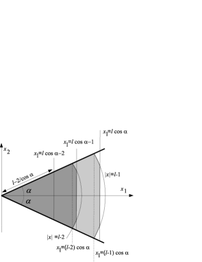
Figure 3: The function $\varphi_{\alpha,\ell}$ vanishes outside the shaded domains, and equals $1$ in the dark shaded domain.

Finally, we set

$$\psi_{\alpha,\ell}(x):=\varphi_{\alpha,\ell}(x)U_{\alpha}(x)\,,$$

where $U_{\alpha}$ is defined in (4). Using the properties (19) and a simple direct computation one obtains:

Lemma 3.4.

The function $\psi_{\alpha,\ell}$ belongs to the domain of $H_{\alpha}\,$, and the following estimates are valid as $\ell\to+\infty\,$:

$$\|\psi_{\alpha,\ell}\|^{2}_{L^{2}(S_{\alpha})} =1+O(\ell e^{-2\beta\ell\cot\alpha})\,,$$ (20)

$$\big{\|}(-\Delta-E_{\alpha})\psi_{\alpha,\ell}\big{\|}^{2}_{L^{2}(S_{\alpha})} =O(\ell e^{-2\beta\ell\cot\alpha})\,.$$ (21)

Now let us choose the maximal constant $\tau>1$ such that the two isosceles triangles $\Theta_{1}(\tau L)$ and $\Theta_{2}(\tau L)$ with the side length $\tau L$ and the vertex angle $\omega$ spanned at the boundary of $\Omega$ near respectively $A_{1}$ and $A_{2}$ are included in $\Omega$. More precisely,

$$\tau:=\begin{cases}\dfrac{1}{\cos\omega},&\omega\in\Big{(}0,\dfrac{\pi}{3}\Big{)}\,,\\[6.0pt] 2,&\omega\in\Big{[}\dfrac{\pi}{2},\pi\Big{)}\end{cases}$$ (22)

see Figure 4.

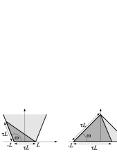
Figure 4: The choice of the constant $\tau$.

Consider the functions

$$\psi_{j}(x)=v_{j}(x)U_{j}(x)\quad\text{with}\quad v_{j}(x):=\varphi_{\alpha,\tau L}(R_{j}x)\,,\quad j=1,2\,.$$

By Proposition 3.2 we can find $\delta>0$ such that the interval $I:=(E_{\alpha}-\delta,E_{\alpha}+\delta)$ contains exactly two eigenvalues of $H_{L}$ and the larger interval $(E_{\alpha}-2\delta,E_{\alpha}+2\delta)$ does not contain any further spectrum for large $L$.

Let $E$ denote the subspace spanned by $\psi_{j}$, $j=1,2$, and $F$ denote the spectral subspace of $H_{L}$ corresponding to $I\,$. We are going to estimate the distances $d(E,F)$ and $d(F,E)$ between these two subspaces, see Subsection 2.1.

Lemma 3.5.

For the Gramian matrix $G:=(g_{jk})=\big{(}\langle\psi_{j},\psi_{k}\rangle\big{)}$ we have

$$g_{jk}=\delta_{jk}+O(Le^{-2\beta L\cot\alpha})\,,\quad j,k=1,2.$$

Furthermore, $g_{11}=g_{22}$ and $g_{12}=g_{21}\,$.

Proof.

The identities for the coefficients follow from the considerations of symmetry. It follows from Lemma 3.4 that

$$\|\psi_{j}\|^{2}=1+O(Le^{-2\tau\beta L\cot\alpha})\quad\text{ for }j=1,2\,.$$

On the other hand, using the explicit expressions (13) for $U_{j}$ , we obtain

$$\psi_{1}(x_{1},x_{2})\psi_{2}(x_{1},x_{2})=2\beta^{2}\dfrac{\cos\alpha}{\sin^{3}\alpha}\varphi_{\alpha,\tau L}(R_{1}x)\varphi_{\alpha,\tau L}(R_{2}x)\exp\big{(}-2\beta L\cot\alpha)\exp(-2\beta x_{2}\big{)}\,.$$

Using the properties (19) we have

$$\langle\psi_{1},\psi_{2}\rangle=O(Le^{-2\beta L\cot\alpha})\,.$$

As $\tau>1$ by (22), this gives the result. ∎

Lemma 3.6.

For large $L$ there holds

$$d(E,F)=d(F,E)=O(\sqrt{L}e^{-\beta\tau L\cot\alpha})\,.$$

Proof.

Let us show first the desired estimate for $d(E,F)$. By Lemma 3.4, we have

$$\big{\|}(H_{L}-E_{\alpha})\psi_{j}\big{\|}=O(\sqrt{L}e^{-\beta\tau L\cot\alpha})\,.$$

Using Proposition 2.3 for the previously chosen interval $I$ and applying Lemma 3.5 gives the result.

We will now show that $d(F,E)<1$ for large $L$, then by Proposition 2.2 it will follow that $d(F,E)=d(E,F)$.

Let $\varphi:\mathbb{R}\to\mathbb{R}$ be a $C^{\infty}$ function such that $\varphi(t)=1$ for $t$ near $0$ and $\varphi(t)=0$ for $t>\frac{1}{2}$ and introduce

$$\chi_{j}(x):=\varphi\Big{(}\dfrac{|x-A_{j}|}{L}\Big{)},\quad j=1,2\,,\quad\chi_{0}:=1-\chi_{1}-\chi_{2}\,.$$

Let $u_{k}$ be a normalized eigenfunction of $H_{L}$ associated with $E_{k}(L)\,$, $k=1,2$. We know (Proposition 3.2) that $E_{k}(L)$ tends to $E_{\alpha}$ as $L\to+\infty$, so Proposition 2.8 is applicable to $u_{k}$. In particular, for some $\sigma>0$ we have

$$\|\chi_{0}u_{k}\|_{L^{2}(\Omega)}=O(e^{-\sigma L})\,.$$

Furthermore, using Proposition 2.6 we check that $\chi_{j}u_{k}\in D(H_{L})$ and that

$$\big{\|}(H_{L}-E_{\alpha})(\chi_{j}u_{k})\big{\|}_{L^{2}(\Omega)}=\big{\|}(-\Delta-E_{\alpha})(\chi_{j}u_{k})\big{\|}_{L^{2}(\Omega)}\\ =\big{\|}-(\Delta\chi_{j})u_{k}-2\nabla\chi_{j}\nabla u_{k}\big{\|}_{L^{2}(\Omega)}=O(e^{-\sigma^{\prime}L})\,,$$

for some $\sigma^{\prime}>0\,$, and by taking the minimum we may assume that $\sigma=\sigma^{\prime}\,$. The last estimate can be also rewritten as an estimate in $L^{2}(\Sigma_{j})$, and we conclude that there exists $L_{*}>0$ and $C>0$ such that

$$\big{\|}(-\Delta-E_{\alpha})(\chi_{j}u_{k})\big{\|}_{L^{2}(\Sigma_{j})}\leq C\,e^{-\sigma L}$$

for $L>L_{*}\,$.

Now let us pick any $\sigma_{0}\in(0,\sigma)$ and split the set $\{L:L>L_{*}\}$ into two disjoint parts $I_{1}$ and $I_{2}$ as follows. We say that $L\in I_{1}$ if $\|\chi_{j}u_{k}\|_{L^{2}(\Omega)}\equiv\|\chi_{j}u_{k}\|_{L^{2}(\Sigma_{j})}\leq e^{-\sigma_{0}L}\,$. Therefore, for $L\in I_{2}$ we have $\|\chi_{j}u_{k}\|_{L^{2}(\Sigma_{j})}\geq e^{-\sigma_{0}L}\,$. We check again that $\chi_{j}u_{k}\in D(M_{j})\,$, so by applying Proposition 2.2 to the operator $M_{j}$ we conclude that

$$d\big{(}\operatorname{Span}(\chi_{j}u_{k}),\ker(M_{j}-E_{\alpha})\big{)}\leq C_{0}\,e^{-(\sigma-\sigma_{0})L}\,,\quad C_{0}>0\,,$$

which means that one can find $a_{jk}\in\mathbb{R}$ such that

$$\|\chi_{j}u_{k}-a_{jk}U_{j}\|_{L^{2}(\Sigma_{j})}\leq C_{0}\,e^{-(\sigma-\sigma_{0})L}\,,$$

and

$$|a_{jk}|\leq 1+C_{0}\,e^{-(\sigma-\sigma_{0})L}\,.$$

On the other hand, one can find $\sigma_{1}>0$ such that

$$\|U_{j}-\psi_{j}\|_{L^{2}(\Omega)}\equiv\|U_{j}-\psi_{j}\|_{L^{2}(\Sigma_{j})}=\|(1-v_{j})U_{j}\|_{L^{2}(\Sigma_{j})}\leq C_{1}\,e^{-\sigma_{1}L}\,.$$

Therefore, writing $\sigma_{2}:=\min(\sigma_{1},\,\sigma-\sigma_{0})\,$, we have

$$\|\chi_{j}u_{k}-a_{j}\psi_{j}\|_{L^{2}(\Omega)}=\|\chi_{j}u_{k}-a_{jk}\psi_{j}\|_{L^{2}(\Sigma_{j})}\leq C_{2}\,e^{-\sigma_{2}L}\text{ for all }L\in I_{2}\,.$$

By choosing $\sigma_{*}:=\min(\sigma_{0},\sigma_{2})\,$, we conclude that, for any sufficiently large $L$, we can find $a_{j}\in\mathbb{R}$ with $|a_{j}|\leq 1+O(e^{-\sigma_{*}L})\,$, such that

$$\|\chi_{j}u_{k}-a_{jk}\psi_{j}\|_{L^{2}(\Omega)}=O(e^{-\sigma_{*}L})\,.$$

For $L\in I_{1}$ we can simply take $a_{jk}=0\,$. We have then

$$u_{k}=\sum_{j=0}^{2}\chi_{j}u_{k}=\sum_{j=1}^{2}a_{jk}\psi_{j}+O(e^{-\sigma_{*}L})\text{ in }L^{2}(\Omega)\,.$$

As the functions $u_{k}$, $k=1,2$, form an orthonormal basis in $F$, we have $d(F,E)=O(e^{-\sigma_{*}L})<1$ for large $L$. ∎

3.4 Coupling between corners

Recall that $P_{E}$ denotes the orthogonal projection on $E$ in $L^{2}(\Omega)$. In addition, we denote by $\Pi_{E}$ the projection on $E$ in $L^{2}(\Omega)$ along $F^{\perp}$. The following lemma essentially reproduces Lemma 2.8 in [HS1]. We give the proof for the sake of completeness.

Lemma 3.7.

For sufficiently large $L$ we have

$$\|\Pi_{E}-P_{E}\|=O(\sqrt{L}e^{-\beta\tau L\cot\alpha})\,.$$

Furthermore, we have the following identities:

• $\Pi_{E}=\Pi_{E}P_{F}$ ,

• the inverse of $K:=(\Pi_{E}:F\to E)$ is $K^{-1}:=(P_{F}:E\to F)\,$,

• $(H_{L}:F\to F)=K^{-1}(\Pi_{E}H_{L}:E\to E)K\,$.

Proof.

By Lemma 3.6 we can write $F=\{x+Ax:x\in E\}$, where $A$ is a bounded linear operator acting from $E$ to $E^{\perp}$ with $\|A\|=O(\sqrt{L}e^{-\beta cL\cot\alpha})$. Then $F^{\perp}=\{y-A^{*}y:y\in E^{\perp}\}$. Furthermore, if $z=x+y$ with $x\in E$ and $y\in E^{\perp}$, then $P_{E}z=x$ and $\Pi_{E}z=\widetilde{x}$, where $\widetilde{x}$ is the vector from $E$ satisfying $\widetilde{x}-(x+y)\in F^{\perp}$, which can be rewritten as $\widetilde{x}-(x+y)=A^{*}\widetilde{y}-\widetilde{y}$ for some $\widetilde{y}\in E^{\perp}$. Considering separately the terms in $E$ and $E^{\perp}$ we arrive at the system $\widetilde{x}-x=A^{*}\widetilde{y}$, $y=\widetilde{y}$, which implies

$$\big{\|}(P_{E}-\Pi_{E})z\big{\|}=\|x-\widetilde{x}\|\leq\|A\|\cdot\|y\|\leq\|A\|\cdot\|z\|$$

and proves the norm estimate.

Let us check the identities. To prove (a) we write $\Pi_{E}=\Pi_{E}(P_{F}+P_{F^{\perp}})$ and note that $\Pi_{E}P_{F^{\perp}}=0$. To prove (b), we observe first that the existence of the inverses follows from Proposition 2.2. Now let us take any $z\in F$. It is uniquely represented as $z=x+y$ with $x\in E$ and $y\in F^{\perp}$, and $P_{E}z=x$. On the other hand, one has $\Pi_{F}x=z$, which proves the identity (b).

Furthermore, $\Pi_{E}H_{L}=\Pi_{E}H_{L}(P_{F}+P_{F^{\perp}})=\Pi_{E}H_{L}P_{F}+\Pi_{E}P_{F^{\perp}}H_{L}\,$. Using again $\Pi_{E}P_{F^{\perp}}=0\,$, we conclude that $\Pi_{E}H_{L}u=\Pi_{E}H_{L}P_{F}u$ for any $u\in E\,$. Finally, as $H_{L}P_{F}u\in F$ for any $u\in E$, we have

$$(\Pi_{E}H_{L}:E\to E)=(\Pi_{E}:F\to E)(H_{L}:F\to F)(P_{F}:E\to F)\,.$$

Combining with (b) leads to (c). ∎

Lemma 3.8.

The matrix $M$ of $\Pi_{E}H_{L}:E\to E$ in the basis $(\psi_{1},\psi_{2})$ is

$$M=\begin{pmatrix}E_{\alpha}&w_{12}\\ w_{21}&E_{\alpha}\end{pmatrix}+O(L^{3/2}e^{-2\beta\tau L\cot\alpha})\,,\quad L\to+\infty,$$

where we denote

$$w_{jk}:=\iint_{\Omega}v_{k}(U_{j}\nabla U_{k}-U_{k}\nabla U_{j})\nabla v_{j}\,dx\,.$$

Proof.

The proof follows the scheme of Theorem 3.9 in [HS1]. We have

$$P_{E}u=\sum_{j,k=1}^{2}c_{jk}\langle\psi_{k},u\rangle\psi_{j}\,,$$

where $c_{jk}$ are the coefficients satisfying

$$\sum_{j,k=1}^{2}c_{jk}\langle\psi_{k},\psi_{\ell}\rangle\psi_{j}=\psi_{\ell}\,,\quad\ell=1,2\,,\text{ i.e. }\sum_{k=1}^{2}c_{jk}\langle\psi_{k},\psi_{\ell}\rangle=\delta_{jl}\,,\quad\ell=1,2\,.$$

In other words, $(c_{jk})=G^{-1}$, where $G$ is the Gramian matrix of $(\psi_{j})$, and in virtue of Lemma 3.5 we have

$$c_{jk}=\delta_{jk}+O(Le^{-2\beta L\cot\alpha})\,.$$

Therefore, if we introduce another operator $\widehat{\Pi}$ by $\widehat{\Pi}u=\sum_{j=1}^{2}\langle\psi_{j},u\rangle\psi_{j}\,$, we have

$$\|P_{E}-\widehat{\Pi}\|=O(Le^{-2\beta L\cot\alpha})\,.$$

Combining with Lemma 3.7 we obtain

$$\|\Pi_{E}-\widehat{\Pi}\|=O(Le^{-\beta\tau L\cot\alpha})\,.$$

Here we used the inequality $\tau\leq 2\,$, see (22).

Now, using the structure of $\psi_{j}=v_{j}U_{j}$ we have

$$H_{L}\psi_{j}=E_{\alpha}\psi_{j}-2\nabla v_{j}\nabla U_{j}-(\Delta v_{j})U_{j}\,.$$

The $L^{2}(\Omega)$-norms of two last terms on the right hand side are $O(\sqrt{L}e^{-\beta\tau L\cot\alpha})\,$, which gives

$$\Pi_{E}H_{L}\psi_{j} =\Pi_{E}\big{(}E_{\alpha}\psi_{j}\big{)}+\widehat{\Pi}\big{(}-2\nabla v_{j}\nabla U_{j}-(\Delta v_{j})U_{j}\big{)}$$ (23)

$$\quad+(\Pi_{E}-\widehat{\Pi})\big{(}-2\nabla v_{j}\nabla U_{j}-(\Delta v_{j})U_{j}\big{)}$$

$$=E_{\alpha}\psi_{j}+\widehat{\Pi}\big{(}-2\nabla v_{j}\nabla U_{j}-(\Delta v_{j})U_{j}\big{)}+O(L^{3/2}e^{-2\beta\tau L\cot\alpha})$$

$$=E_{\alpha}\psi_{j}+\sum_{k=1}^{2}b_{jk}\psi_{k}+O(L^{3/2}e^{-2\beta\tau L\cot\alpha}).$$

with

$$b_{jk}:=-\iint_{\Omega}\big{(}2\nabla v_{j}\nabla U_{j}+(\Delta v_{j})U_{j}\big{)}\psi_{k}\,dx=-\iint_{\Omega}\big{(}2\nabla v_{j}\nabla U_{j}+(\Delta v_{j})U_{j}\big{)}v_{k}U_{k}\,dx.$$

Using the Green-Riemann formula (7) we have

$$\iint_{\Omega}(-\Delta v_{j})U_{j}\big{)}v_{k}U_{k}\,dx=\iint_{\Omega}\nabla v_{j}\nabla(U_{j}U_{k}v_{k})\,dx-\int_{\partial\Omega}\dfrac{\partial v_{j}}{\partial n}U_{j}U_{k}v_{k}\,ds\\ =\iint_{\Omega}U_{j}U_{k}\nabla v_{j}\nabla v_{k}\,dx+\iint_{\Omega}U_{j}v_{k}\nabla v_{j}\nabla U_{k}\,dx+\iint_{\Omega}v_{k}U_{k}\nabla v_{j}\nabla U_{j}\,dx\,,$$

which gives

$$b_{jk}=\delta_{jk}w_{jk}+\varepsilon_{jk},\quad\varepsilon_{jk}:=\iint_{\Omega}U_{j}U_{k}\nabla v_{j}\nabla v_{k}\,dx\,.$$ (24)

Note that

$$U_{1}(x_{1},x_{2})U_{2}(x_{1},x_{2})=\dfrac{2\beta^{2}\cos\alpha}{\sin^{3}\alpha}\exp\big{(}-2\beta L\cot\alpha)\exp(-2\beta x_{2}\big{)}$$ (25)

and that $\nabla v_{1}\nabla v_{2}$ is supported in a parallelogram of size $O(1)$ in which the value of $x_{2}$ is at least

$$S:=(\tau-1)L\cot\alpha-2/\sin\alpha\,,$$

see Figure 5. Therefore,

$$\varepsilon_{12}=\varepsilon_{21}=O(e^{-2\tau\beta L\cot\alpha})\,.$$

On the other hand, by Lemma 3.4 we have

$$\varepsilon_{11}=\varepsilon_{22}=O(Le^{-2\beta\tau L\cot\alpha})\,.$$

Substituting these estimates into (24) and then into (23) leads to the conclusion. ∎

Lemma 3.9.

There holds

$$w:=w_{12}=w_{21}=\dfrac{2\beta^{2}\cos^{2}\alpha}{\sin^{4}\alpha}e^{-2\beta L\cot\alpha}+O\big{(}Le^{-2\beta\tau L\cot\alpha}\big{)}\,.$$

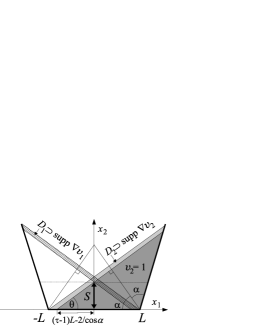
Figure 5: Computation of $S$. In the dark shaded domain there holds $v_{2}=1\,$, cf. Figure 3. We have $\theta=\frac{\pi}{2}-\alpha$ and, hence, $S=\big{(}(\tau-1)L-2\cos\alpha\big{)}\tan\theta\equiv(\tau-1)L\cot\alpha-2/\sin\alpha\,.$

Proof.

The equality $w_{12}=w_{21}$ follows from the symmetry considerations. Furthermore, we have the equality

$$U_{1}\nabla U_{2}-U_{2}\nabla U_{1}=2\beta\cot\alpha\begin{pmatrix}1\\ 0\end{pmatrix}U_{1}U_{2}\,.$$

Substituting the expression for $U_{1}U_{2}$ from (25) we obtain

$$w_{12}=\dfrac{4\beta^{3}\cos^{2}\alpha}{\sin^{4}\alpha}e^{-2\beta L\cot\alpha}A\,,\quad A:=\iint_{\Omega}e^{-2\beta x_{2}}v_{2}\dfrac{\partial v_{1}}{\partial x_{1}}\,dx\,.$$

Using the explicit construction of $v_{1}$ and $v_{2}$ we can see that, for $x_{2}<S:=(\tau-1)L\cot\alpha-2/\sin\alpha\,$, we have the following property: if $(x_{1},x_{2})\in\operatorname{supp}\nabla v_{1}$, then $v_{2}(x_{1},x_{2})=1\,$, see Figure 5. This allows one to estimate $A$ by

$$A=\iint_{\Omega\cap\{x_{2}\leq S\}}e^{-2\beta x_{2}}\dfrac{\partial v_{1}(x_{1},x_{2})}{\partial x_{1}}\,dx+O\big{(}Le^{-2\beta(\tau-1)L\cot\alpha}\big{)}\,.$$

On the other hand, by Fubini

$$\iint_{\Omega\cap\{x_{2}\leq S\}}e^{-2\beta x_{2}}\dfrac{\partial v_{1}(x_{1},x_{2})}{\partial x_{1}}dx=\int_{0}^{S}e^{-2\beta x_{2}}\bigg{(}\int\dfrac{\partial v_{1}(x_{1},x_{2})}{\partial x_{1}}dx_{1}\bigg{)}dx_{2}.$$

The interior integral is equal to $1$ for any $x_{2}$, which finally gives

$$A=\int_{0}^{S}e^{-2\beta x_{2}}dx_{2}+O\big{(}Le^{-2\beta(\tau-1)L\cot\alpha}\big{)}=\dfrac{1}{2\beta}+O\big{(}Le^{-2\beta(\tau-1)L\cot\alpha}\big{)}.$$

∎

Lemma 3.10.

The matrix $N$ of $\Pi_{E}H_{L}:E\to E$ in the orthonormal basis

$$\phi_{k}=\sum_{j=1}^{2}\psi_{j}\sigma_{jk},\quad k=1,2,\quad\sigma:=(\sigma_{jk}):=\sqrt{G^{-1}}\,,$$

has the form

$$N=N_{0}+O(L^{2}e^{-2\beta\tau L\cot\alpha})\quad\text{with}\quad N_{0}=\begin{pmatrix}E_{\alpha}&w\\ w&E_{\alpha}\end{pmatrix}\,.$$

Here $G$ is the Gramian matrix from Lemma 3.5.

Proof.

Due to Lemma 3.5 we have $G=I+T$ with $T=O(Le^{-2\beta L\cot\alpha})$, which shows that

$$\sigma=I-\frac{1}{2}T+O(L^{2}e^{-4\beta L\cot\alpha})\,,\quad\sigma^{-1}=I+\frac{1}{2}T+O(L^{2}e^{-4\beta L\cot\alpha})\,.$$

On the other hand, using the matrix $M$ from Lemma 3.8, we have $N=\sigma^{-1}M\sigma$. So we get

$$N =\Big{(}I+\frac{1}{2}T+O(L^{2}e^{-4\beta L\cot\alpha}\Big{)}\Big{(}E_{\alpha}+\begin{pmatrix}0&w\\ w&0\end{pmatrix}+O(L^{3/2}e^{-2\beta tL\cot\alpha})\Big{)}$$

$$\quad\times\Big{(}I-\frac{1}{2}T+O(L^{2}e^{-4\beta L\cot\alpha}\Big{)}$$

$$=\begin{pmatrix}E_{\alpha}&w\\ w&E_{\alpha}\end{pmatrix}+\dfrac{1}{2}\bigg{[}T\begin{pmatrix}0&w\\ w&0\end{pmatrix}-\begin{pmatrix}0&w\\ w&0\end{pmatrix}T\bigg{]}+O(L^{2}e^{-2\beta\tau L\cot\alpha})\,.$$

The term in the square brackets equals zero due to Lemma 3.5, and this achieves the proof. ∎

Proof of Theorem 1.1.

Now we are able to finish the proof of the main theorem. The eigenvalues of the matrix $N_{0}$ from Lemma 3.10 are $E_{\pm}:=E_{\alpha}\pm|w|$, and in view of Lemma 3.9 we have

$$E_{\pm}=-\dfrac{\beta^{2}}{\sin^{2}\alpha}\pm\dfrac{2\beta^{2}\cos^{2}\alpha}{\sin^{4}\alpha}e^{-2\beta L\cot\alpha}+O\big{(}Le^{-2\beta\tau L\cot\alpha}\big{)}\,.$$

By Lemma 3.9, these numbers $E_{\pm}$ coincide up to $O(L^{2}e^{-2\beta\tau L\cot\alpha})$ with the eigenvalues of $H_{L}$ in $I$, which are exactly $E_{1}(L)$ and $E_{2}(L)\,$. It remains to apply elementary trigonometric identities to pass from $\alpha=\omega/2$ to $\omega\,$. ∎

4 Conclusion

To conclude this article, let us add a few remarks.

Remark 4.1.

The family of operators $H_{L}$ includes one case in which one can separate the variables, namely, the case $\omega=\frac{\pi}{2}\,$, for which the estimate of Theorem 1.1 takes the form

$$E_{1/2}(L)=-2\beta^{2}\mp 4\beta^{2}e^{-2\beta L}+O(L^{2}e^{-4\beta L})\,.$$ (26)

On the other hand, one can represent $H_{L}=A\otimes 1+1\otimes B_{L}$, where $A$ and $B_{L}$ are operators in $L^{2}(0,\infty)$ and $L^{2}(-L,L)$ respectively:

$$Au=-u^{\prime\prime},\quad D(A)=\big{\{}u\in H^{2}(0,\infty):u^{\prime}(0)+\beta u(0)=0\big{\}}\,,$$

$$B_{L}v=-v^{\prime\prime}\,,\quad D(B_{L})=\big{\{}v\in H^{2}(-L,L):v^{\prime}(-L)+\beta v(-L)=v^{\prime}(L)-\beta v(L)=0\big{\}}\,.$$

One easily computes

$$\operatorname{spec}A=\{-\beta^{2}\}\cup[0,+\infty)\,.$$

On the other hand, $B_{L}$ has a compact resolvent and, if one denotes its eigenvalues by $\varepsilon_{j}(L)$, then

$$E_{j}(L)=-\beta^{2}+\varepsilon_{j}(L)\,.$$

The behavior of $\varepsilon_{j}(L)$, $j=1,2$, can be studied in a rather explicit way by using the 1D nature of the problem, see Proposition A.3 in the appendix, and one gets

$$E_{1/2}(L)=-2\beta^{2}\mp 4\beta^{2}e^{-2\beta L}+8\beta^{2}(2\beta L-1)e^{-4\beta L}+O(L^{2}e^{-6\beta L})\,,\\$$

One observes that the remainder estimate in our asymptotics (26) only differs by the factor $L$ from the exact one.

Remark 4.2.

One can also consider the case $\omega=\frac{\pi}{3}\,$, i.e. the case of the equilateral triangle. In this case one has an interaction between the three corners. The above scheme works in essentially the same way; see also [HS2] and [FH, Section 16.2] for the general discussion. One can prove that, for sufficiently large $L$, there exists a bijection $\sigma$ between the three lowest eigenvalues of $H_{L}$ and the three eigenvalues of the matrix

$$N_{0}=\begin{pmatrix}E_{\alpha}&w&w\\ w&E_{\alpha}&w\\ w&w&E_{\alpha}\end{pmatrix},\quad w=24\,\beta^{2}e^{-2\sqrt{3}L}\,,$$

such that $\sigma(E)=E+O(L^{2}e^{-4\sqrt{3}\beta L})\,$.

Note that the eigenvalues of $N_{0}$ are $E_{\alpha}-w$ (simple) and $E_{\alpha}+w$ (double), which means that the three lowest eigenvalues of $H_{L}$ behave as

$$E_{1}(L) =-4\,\beta^{2}-24\,\beta^{2}e^{-2\sqrt{3}L}+O(L^{2}e^{-4\sqrt{3}\beta L})\,,$$

$$E_{j}(L) =-4\,\beta^{2}+24\,\beta^{2}e^{-2\sqrt{3}L}+O(L^{2}e^{-4\sqrt{3}\beta L})\,,\quad j=2,3\,,$$

i.e. no splitting is visible between $E_{2}$ and $E_{3}\,$. Actually there is no surprise, as a symmetry argument as well as the explicit formulas from [McC, Section 7] show that

$$E_{2}(L)=E_{3}(L).$$

Remark 4.3.

One may see from the proof that the result admits direct extensions to a little bit more general domains. Namely, assume that $\Omega=L\Omega^{\prime}$ with some $L$-independent $\Omega^{\prime}$ and such that $\Omega$ coincides with $\Omega_{L}$ near the axis $Ox_{1}$ in the following sense: one still can construct the triangles $\Theta_{j}(\tau L)$, $j=1,2$, as in Subsection 3.3 for some $\tau>1$, and $\Omega$ does not contain any further corner whose opening is smaller or equal to $\omega$. Then Theorem 1.1 is valid for the first two eigenvalues of $H(\Omega,\beta)$ with $\delta=2(\tau-1)$. It would be interesting to know if any result of this kind can be obtained for more general domains and more general relative positions of the corners. For the smooth domains, one may expect that the role of the corners is played by the points of the boundary at which the curvature is maximal [EMP, P], which gives rise to similar questions. This is actually the case for surface superconductivity, see [FH] and references therein.

Remark 4.4.

Our considerations were in part stimulated by the paper [BND] which studies the asymptotic behavior of the eigenvalues of the magnetic Neumann Laplacians in curvilinear polygons, but in our case we were able to obtain a more precise result due to the fact that we know the exact eigenfunction of an infinite sector. One may wonder if our machinery can help to progress in the problem of [BND]. We note that both the magnetic Neumann Laplacian and the Robin Laplacian appear as approximate models in the theory of surface superconductivity and are closely related to the computation of the critical temperature [GS, HS1].

Appendix A 1D Robin problem

In this section, we study the one-dimensional Robin problem. The expressions obtained have their own interest, but some estimates can be used to obtain a better estimate for the analysis of the two-dimensional situation, as explained in Remark 4.1.

Lemma A.1.

For $\beta>0$ and $\ell>0$, denote by $N_{\beta,\ell}$ the operator acting in $L^{2}(0,\ell)$ as $f\mapsto-f^{\prime\prime}$ on the functions $f\in H^{2}(0,\ell)$ satisfying the boundary conditions $f^{\prime}(0)=0$ and $f^{\prime}(\ell)=\beta f(\ell)$. Then the lowest eigenvalue $E_{N}(\beta,\ell)$ is the unique strictly negative eigenvalue, and

$$E_{N}(\beta,\ell)=-\beta^{2}-4\beta^{2}e^{-2\beta\ell}+8\beta^{2}(2\beta\ell-1)e^{-4\beta\ell}+O(\ell^{2}e^{-6\beta\ell})\,\text{ as $\ell$ tends to $+\infty$\,,}$$ (27)

and the associated eigenfunction is $x\mapsto\cosh(\sqrt{-E_{N}(\beta,\ell)}x)\,$.

Proof.

Let us write $E_{N}(\beta,\ell)=-k^{2}$ with $k>0$. The associated eigenfunction $f$ must be of the form $f(x)=Ae^{kx}+Be^{-kx}$ with some $(A,B)\in\mathbb{R}^{2}\setminus\big{\{}(0,0)\big{\}}$. Taking into the account the boundary conditions we get the linear system

$$A-B=0\,,\,(k-\beta)e^{k\ell}A-(k+\beta)e^{-k\ell}B=0\,.$$

It follows that $f(x)=2B\cosh(kx)$. The system has non-trivial solutions iff

$$(k-\beta)e^{k\ell}=(k+\beta)e^{-k\ell}\,.$$ (28)

This can be rewritten as $k\ell\tanh(k\ell)=\beta\ell$. One easily checks that the function

$$(0,+\infty)\ni t\mapsto t\tanh t\in(0,+\infty)$$

is a bijection, which means that the solution $k$ to  (28) is defined uniquely, which shows that we have exactly one negative eigenvalue.

To calculate its asymptotics, we first take into account the signs of all terms in (28), which gives $k>\beta\,$.

Rewriting (28) in the form

$$(k-\beta)=2\beta e^{-2k\ell}/(1-e^{-2k\ell})=2\beta e^{-2\beta\ell}e^{-2(k-\beta)\ell}/(1-e^{-2(k-\beta)\ell}e^{-2\beta\ell})\,,$$

we get that

$$k-\beta=O(e^{-2\beta\ell})\,.$$ (29)

It follows also from (28) that

$$k=\dfrac{1+e^{-2k\ell}}{1-e^{-2k\ell}}\beta=\big{(}1+2e^{-2k\ell}+O(e^{-4k\ell})\big{)}\beta\,,\quad\ell\to+\infty\,.$$ (30)

Implementing (29), we infer that

$$k=\big{(}1+2e^{-2\beta\ell}+O(\ell e^{-4\beta\ell})\big{)}\beta=\beta+2\beta e^{-2\beta\ell}+O(\ell e^{-4\beta\ell})\,.$$ (31)

By taking an additional term in (30),

$$k=\dfrac{1+e^{-2k\ell}}{1-e^{-2k\ell}}\beta=\big{(}1+2e^{-2k\ell}+2e^{-4k\ell}+O(e^{-6k\ell})\big{)}\beta\,,\quad\ell\to+\infty\,,$$

and by using (31) one gets

$$k=\beta+2\beta e^{-2\beta\ell}+2\beta(1-4\beta\ell)e^{-4\beta\ell}+O(\ell^{2}e^{-6\beta\ell})\,.$$ (32)

Computing $E=-k^{2}$ gives the result. ∎

Lemma A.2.

For $\beta>0$ and $\ell>0$, denote by $D_{\beta,\ell}$ the operator acting in $L^{2}(0,\ell)$ as $f\mapsto-f^{\prime\prime}$ on the functions $f\in H^{2}(0,\ell)$ satisfying the boundary conditions $f(0)=0$ and $f^{\prime}(\ell)=\beta f(\ell)$, and let $E_{D}(\beta,\ell)$ denote its lowest eigenvalue. Then $E_{D}(\beta,\ell)<0$ iff $\beta\ell>1$, and in that case it is the only negative eigenvalue. Furthermore,

$$E_{D}(\beta,\ell)=-\beta^{2}+4\beta^{2}e^{-2\beta\ell}+8\beta^{2}(2\beta\ell-1)e^{-4\beta\ell}+O(\ell^{2}e^{-6\beta\ell})\text{ as $\ell$ tends to $+\infty\,$,}$$ (33)

and the associated eigenfunction is $x\mapsto\sinh(\sqrt{-E_{D}(\beta,\ell)}x)$.

Proof.

Let us write $E_{D}(\beta,\ell)=-k^{2}$ with $k>0$. The associated eigenfunction $f$ is of the form $f=Ae^{kx}+Be^{-kx}$ with some $(A,B)\in\mathbb{R}^{2}\setminus\big{\{}(0,0)\big{\}}$. Taking into the account the boundary conditions we get the linear system

$$A+B=0\,,\,(k-\beta)e^{k\ell}A-(k+\beta)e^{-k\ell}B=0\,,$$

which gives the representation $f(x)=2A\sinh(kx)$. Non-trivial solutions exist iff

$$(\beta+k)e^{-k\ell}=(\beta-k)e^{k\ell}\,.$$ (34)

The preceding equation can be rewritten as

$$k\ell\coth(k\ell)=\beta\ell\,.$$

One easily checks that the function

$$(0,+\infty)\ni t\mapsto t\coth t\in(1,+\infty)$$

is a bijection, which shows that (34) has a solution iff $\beta\ell>1$, and if it is the case, the solution is unique, which gives in turn the unicity of the negative eigenvalue.

For the rest of the proof we assume that

$$\beta\ell>1\,.$$

By considering the signs of both sides in (34) we conclude that $k<\beta$. Furthermore, we may rewrite (34) as $g(k)=0$ with

$$g(k)=\log(\beta+k)-\log(\beta-k)-2k\ell\,.$$

We have $g(0+)=0$ and $g(\beta-)=+\infty\,$. The equation $g^{\prime}(k)=0$ takes the form

$$\beta^{2}-k^{2}=\dfrac{\beta}{\ell},$$

and its unique solution is

$$k^{*}=\beta\sqrt{1-\dfrac{1}{\beta\ell}}\,.$$

It follows that the equation $g(k)=0$ has a unique solution $k$ in $(0,\beta)$ and that $k\in(k^{*},\beta)\,$. On the other hand, we obtain the estimate

$$k^{*}>\beta\Big{(}1-\dfrac{1}{\beta\ell}\Big{)}=\beta-\dfrac{1}{\ell}.$$

Hence, the solution of $g(k)=0$ satisfies

$$\beta-\dfrac{1}{\ell}<k<\beta\,.$$ (35)

We rewrite (34) in the form

$$\beta-k=\dfrac{2k}{e^{2k\ell}-1}\,.$$

and we deduce with the help of (35) that

$$\beta-k=O(e^{-2\beta\ell})\text{ as }\ell\rightarrow+\infty.$$

By going through the same steps as in the proof of Lemma A.1, one gets the result. ∎

Proposition A.3.

For $\beta>0$ and $\ell>0$, let $B_{\ell}$ denote the operator acting in $L^{2}(-\ell,\ell)$ as $f\mapsto-f^{\prime\prime}$ on the functions $f\in H^{2}(-\ell,\ell)$ satisfying the boundary conditions $f^{\prime}(\pm\ell)=\pm\beta f(\pm\ell)\,$, and let $E_{1}(\ell)$ and $E_{2}(\ell)$ be the two lowest eigenvalues, $E_{1}(\ell)<E_{2}(\ell)\,$. Then:

• $E_{1}(\ell)<0\,$,

• $E_{2}(\ell)<0$ iff $\beta\ell>1\,$,

• all other eigenvalues are non-negative.

Furthermore,

$$E_{1}(\ell) =-\beta^{2}-4\beta^{2}e^{-2\beta\ell}+8\beta^{2}(2\beta\ell-1)e^{-4\beta\ell}+O(\ell^{2}e^{-6\beta\ell})\,,$$

$$E_{2}(\ell) =-\beta^{2}+4\beta^{2}e^{-2\beta\ell}+8\beta^{2}(2\beta\ell-1)e^{-4\beta\ell}+O(\ell^{2}e^{-6\beta\ell})\,,$$

as $\ell$ tends to $+\infty$. The respective eigenfunctions $f_{1}$ and $f_{2}$ are

$$f_{1}(x)=\cosh\big{(}\sqrt{-E_{1}(\ell)}x\big{)}\,,\quad f_{2}(x)=\sinh\big{(}\sqrt{-E_{2}(\ell)}x\big{)}\,.$$

Proof.

Let us use the notation of Lemmas A.1 and A.2. Note that:

• $B_{\ell}$ commutes with the reflections with respect to the origin,

• its first eigenfunction $f_{1}$ is non-vanishing and even, hence, $f_{1}^{\prime}(0)=0\,$,

• its second eigenfunction $f_{2}$ has one zero in $(-\ell,\ell)$ and is odd, hence $f_{2}(0)=0\,$.

Therefore, $E_{1}(\ell)=E_{N}(\beta,\ell)$ and $E_{2}(\ell)=E_{D}(\beta,\ell)\,$, and the result follows from Lemmas A.1 and A.2. ∎

References

- [1]
- [A] A. Yu. Anikin: Asymptotic behavior of the Maupertuis action on a libration and tunneling in a double well. Russ. J. Math. Phys. 20: 1 (2013) 1–10.
- [BND] V. Bonnaillie-Noël, M. Dauge: Asymptotics for the low-lying eigenstates of the Schrödinger operator with magnetic field near corners. Ann. Henri Poincaré 7:5 (2006) 899–931.
- [BE] D. Borisov, P. Exner: Exponential splitting of bound states in a waveguide with a pair of distant windows. J. Phys. A: Math. Gen. 37:10 (2004) 3411–3428.
- [BHM] R. M. Brown, P. D. Hislop, and A. Martinez: Lower bounds on the interaction between cavities connected by a thin tube. Duke Math. J. 73:1 (1994) 163–176.
- [BDS] J. Brüning, S. Yu. Dobrokhotov, and E. S. Semenov: Unstable closed trajectories, librations and splitting of the lowest eigenvalues in quantum double well problem. Regul. Chaotic Dyn. 11:2 (2006) 167–180.
- [D] F. Daumer: Equation de Schrödinger dans l’approximation du tight-binding. PhD thesis, University of Nantes, 1990.
- [EMP] P. Exner, A. Minakov, and L. Parnovski: Asymptotic eigenvalue estimates for a Robin problem with a large parameter. To appear in Portugal. Math., preprint 1312.7293 at arXiv.
- [FH] S. Fournais, B. Helffer: Spectral methods in surface superconductivity. Birkhäuser, 2010.
- [FK] P. Freitas, D. Krejčiřík: The first Robin eigenvalue with negative boundary parameter. Preprint 1403.6666 at arXiv.
- [GS] T. Giorgi, R. Smits: Eigenvalue estimates and critical temperature in zero fields for enhanced surface superconductivity. Z. Angew. Math. Phys. 58:2 (2007) 224–245.
- [G] P. Grisvard: Singularities in boundary value problems. Masson, 1992.
- [H] B. Helffer: Semi-classical analysis for the Schrödinger operator and applications. Volume 1336 of Lecture Notes in Mathematics, Springer, Berlin, 1988.
- [HS1] B. Helffer, J. Sjöstrand: Multiple wells in the semi-classical limit I. Commun. PDE 9:4 (1984) 337–408.
- [HS2] B. Helffer, J. Sjöstrand: Puits multiples en limite semi-classique II. Interaction moléculaire. Symétries. Perturbations. Ann. IHP Sec. A: Phys. Théor. 42:2 (1985) 127–212.
- [Ka] A. Kachmar: On the ground state energy for a magnetic Schrödinger operator and the effect of the de Gennes boundary condition. J. Math. Phys. 47: 7 (2006) 072106. Erratum: J. Math. Phys. 48:1 (2007).
- [LOS] A. A. Lacey, J. R. Ockendon, and J. Sabina: Multidimensional reaction diffusion equations with nonlinear boundary conditions. SIAM J. Appl. Math. 58:5 (1998) 1622–1647.
- [LP] M. Levitin, L. Parnovski: On the principal eigenvalue of a Robin problem with a large parameter. Math. Nachr. 281:2 (2008) 272–281.
- [McC] B. J. McCartin: Laplacian eigenstructure of the equilateral triangle. Hikari Ltd., Ruse, 2011.
- [P] K. Pankrashkin: On the asymptotics of the principal eigenvalue for a Robin problem with a large parameter in planar domains. Nanosystems: Phys. Chem. Math. 4:4 (2013) 474–483.