Zero-one-only process: a correlated random walk with a stochastic ratchet

Abstract

The investigation of random walks is central to a variety of stochastic processes in physics, chemistry, and biology. To describe a transport phenomenon, we study a variant of the one-dimensional persistent random walk, which we call a zero-one-only process. It makes a step in the same direction as the previous step with probability $p$, and stops to change the direction with $1-p$. By using the generating-function method, we calculate its characteristic quantities such as the statistical moments and probability of the first return.

I Introduction

The simple random walker is one of the most important conceptual tools in statistical physics. It lies behind our understanding of diffusive motions in thermal equilibrium, and almost every statistical estimate makes use of its properties based on the central limit theorem Grinstead and Snell (1997); Rudnick and Gaspari (2004). It is also useful in the biological context, because it explains many behavioral aspects of micro-organisms swimming in a viscous liquid Purcell (1977). Recent experiments report another biological application of random walks, performed by repair proteins along one-dimensional DNA sequences Gorman et al. (2007); Ramanathan et al. (2009). The experimental results show the followings: First, the net displacements are distributed symmetrically from the starting point. Second, the mean-squared displacement is found to increase linearly with time. These are exactly the characteristics of the simple random walk. Such a diffusive process is found efficient both in energy and time: The proteins slide along DNA without requiring ATP because the process is driven by thermal energy, and the group of repair proteins in a cell would check the entire genome sequence within 3 minutes even if this one-dimensional diffusion was the only scanning mechanism Gorman et al. (2007).

There are also interesting variations of the simple random walk, one of which is the persistent random walk Masoliver et al. (1992); Boguñá et al. (1998); Weiss (2002); Rudnick and Gaspari (2004). The persistent random walker has a ‘memory’ or ‘momentum’ in the sense that it takes a step in the same direction as the previous one with probability, say, $\alpha$, and in the opposite direction with $1-\alpha$. Such dynamics introduces correlation in the walker’s displacements. However, when we talk about its ‘memory’, it should be understood in a rather loose sense, because this model can still be described by a second-order Markovian process, which is essentially memoryless.

The precise way to introduce persistence depends on the detailed mechanism that we are to describe. In this work, we consider a slightly different type of a persistent random walker which has an external state as its position together with an internal state that prescribes its direction. The walker receives as an input a binary string composed of 1 and 0. The former bit acts on the external state, moving the walker by one discrete step in the prescribed direction. The latter, on the other hand, acts only on the internal state with flipping the direction. The point is that there occurs no displacement in the latter situation, differing from the conventional persistent random walk. Therefore, in terms of the displacement, there are three possibilities, i.e., -1, 0, and +1, at each time step. Such persistence as considered in this work due to the separation of internal and external variables is actually possible in some transport phenomena, for example, if the walker has a ratchet, which forces the motion in a particular direction but is controllable by inputs from outside. If the input string is random so that it contains 1 with probability $p$ and 0 with probability $q\equiv 1-p$, our model can be analyzed by solving a second-order Markovian process with the generation-function method. In addition, it is also possible to obtain the generating function for the returning probability in a closed form at $p=q=\frac{1}{2}$.

This work is organized as follows: In the next section, we present analytic results for the movement of this random walker by using the generating-function method. How it returns to the starting point will be discussed in Sec. III. After comparing the analytic results with numerical ones, we conclude this work.

II Master equation

Suppose that the walker wanders along the one-dimensional line from $-\infty$ to $\infty$. Its position is represented by an integer $n$. We assume that the walker starts from the origin, i.e., $n=0$, at time $t=0$. Every time step, the walker reads a bit from an input string which we denote as $\{X(t)\}$ with $X(t)=1$ at probability $p$ and $X(t)=0$ at probability $q(=1-p)$ for $t\geq 1$. The probability for the walker to occupy position $n$ at time $t$ is denoted as $P^{\pm}(n,t)$, where the superscript means the initial direction, $+$ or $-$, of the walker. Our initial condition is such that the walker is located at the origin with the positive direction, as expressed by $P^{+}(n,0)=\delta_{n0}$ and $P^{-}(n,0)=0$. At time $t\geq 1$, we have

$$P^{+}(n,t)=pP^{+}(n-1,t-1)+qP^{-}(n,t-1),$$ (1)

where the first term corresponds to the case with $X(1)=1$, which is equivalent to shifting the walker by one lattice spacing. The second term corresponds to the other case with $X(1)=0$, which amounts to reverting the direction. By the same logic, we have another recursion relation:

$$P^{-}(n,t)=pP^{-}(n+1,t-1)+qP^{+}(n,t-1).$$ (2)

Let us define

$$Q^{\pm}(x,t)\equiv\sum_{n=-\infty}^{\infty}x^{n}P^{\pm}(n,t),$$ (3)

with the initial condition reexpressed as $Q^{+}(x,0)=1$ and $Q^{-}(x,0)=0$. In terms of Eq. (3), we write Eqs. (1) and (2) as

$$\begin{bmatrix}Q^{+}(x,t)\\ Q^{-}(x,t)\end{bmatrix}=\begin{bmatrix}px&q\\ q&px^{-1}\end{bmatrix}\begin{bmatrix}Q^{+}(x,t-1)\\ Q^{-}(x,t-1)\end{bmatrix}.$$ (4)

The eigenvalues of the matrix are $\lambda_{1}=\frac{p(x+x^{-1})-\sqrt{D}}{2}$ and $\lambda_{2}=\frac{p(x+x^{-1})+\sqrt{D}}{2}$ with $D\equiv 4q^{2}+p^{2}(x-x^{-1})^{2}$. A general expression for $Q^{+}(t)$ is obtained by diagonalizing the $2\times 2$ matrix in Eq. (4). Considering the initial condition at $t=0$, we find that

$$Q^{+}(x,t) = 2^{-1-t}\left\{\left[1-\frac{2q+p(x-x^{-1})}{\sqrt{D}}\right]\lambda_{1}^{t}\right.$$ (5)

$$+\left.\left[1+\frac{2q+p(x-x^{-1})}{\sqrt{D}}\right]\lambda_{2}^{t}\right\}.$$

The mean and variance of the position are obtained as

$$\left<n\right>=\frac{p[1-(p-q)^{t}]}{2q}$$ (6)

and

$$\sigma^{2}=\frac{p\left\{4t-p\left[3-4(p-q)^{t}+(p-q)^{2t}+4t\right]\right\}}{4q^{2}}.$$ (7)

In the limit of $t\rightarrow\infty$, we can approximate $\left<n\right>\approx\frac{p}{2q}$ and $\sigma^{2}\approx\left(\frac{p}{q}\right)t$ for $0\leq p<1$. If $p=q=\frac{1}{2}$, in particular, the mean position is obtained as $\left<n\right>=\frac{1}{2}$, and the variance is $\sigma^{2}=t-\frac{3}{4}$ at arbitrary $t$.

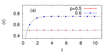
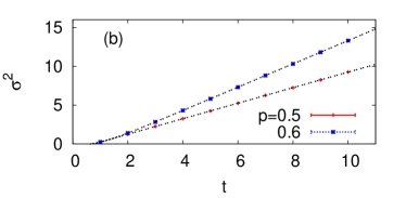
Figure 1: (a) Mean and (b) variance of the position of our persistent random walker at two different values of $p$ as time $t$ varies. The symbols are averages over $3\times 10^{7}$ random samples, while the dotted lines represent the analytic predictions in Eqs. (6) and (7). Error bars are shown but not larger than the symbol size.

Figure 1 depicts numerical results from our Monte Carlo calculation over $3\times 10^{7}$ samples, compared with Eqs. (6) and (7), respectively. The calculated mean and variance fully coincide with the analytic predictions.

III Return probability

Let us now consider the probability of return to the origin at time $t$ and denote it as $u_{t}$. It is convenient to define $u_{0}\equiv 1$. If $t$ is odd, i.e., if $t=2m+1$ with $m=0,1,\ldots$, $u_{t}$ is then given as

$$u_{t} = q\sum_{k=0}^{m}\binom{m}{k}\binom{m}{k}p^{2m-2k}q^{2k}$$

$$= qp^{2m}{}_{2}F_{1}(-m,-m;1;q^{2}/p^{2}),$$

where ${}_{2}F_{1}$ is a hypergeometric function Abramowitz and Stegun (1982). The reason behind Eq. (III) is roughly explained as follows: The summand can be interpreted as pairing two strings of length $m$, for each of which there are $k$ bits of $1$ and the other $(m-k)$ bits of $0$. The probability $q$ in front of the right-hand side of Eq. (III) means that for every such pair, one finds a proper place to insert $0$ so as to bring the walker back to the origin. If we define $b_{t}$ as the probability to occupy $n=-1$ at time $t$, we can establish the following relation:

$$u_{t+1}=pb_{t}+qu_{t},$$ (9)

by conditioning the first bit, $X(1)$. The probability $b_{t}$ turns out to be closely related to the Narayana number MacMahon (1960):

$$N(m,k)=\frac{1}{m}\binom{m}{k}\binom{m}{k-1},$$ (10)

which describes the number of possibilities to have $m$ pairs of correctly matched parentheses with $k$ distinct nestings. If $t=2m+1$, in particular, we find an explicit expression for $b_{t}$ as

$$b_{t} = p\sum_{k=1}^{m}\binom{m}{k}\binom{m}{k-1}p^{2m-2k}q^{2k}$$

$$= mp^{2m-1}q^{2}{}_{2}F_{1}(1-m,-m;2;q^{2}/p^{2}).$$

Plugging Eqs. (III) and (III) into Eq. (9), we have an expression for $u_{t}$ when $t$ is even, too.

Equation (III) simplifies for $p=q=\frac{1}{2}$ due to the following identity in combinatorics:

$$\sum_{k=0}^{m}\binom{m}{k}^{2}=\binom{2m}{m}.$$ (12)

We restrict ourselves to this specific case of $p=q=\frac{1}{2}$ henceforth. Then, the return probability $u_{t}$ found above obeys the following recursion relation:

$$tu_{t}=u_{t-1}+(t-2)u_{t-2}.$$ (13)

Note that $u_{1}=\frac{1}{2}$ because one should get $X(1)=0$ to stay at the origin. Together with $u_{0}\equiv 1$, one can find $u_{t}$ recursively by using Eq. (13). However, it is more useful to introduce the generating function for $u_{t}$ as

$$U(x)\equiv\sum_{t=0}^{\infty}u_{t}x^{t},$$ (14)

and Eq. (13) then reduces to

$$\frac{d}{dx}U(x)=U(x)-\frac{1}{2}+x^{2}\frac{d}{dx}U(x).$$ (15)

This ordinary differential equation is solved to yield

$$U(x)=\frac{1}{2}\left(\sqrt{\frac{1+x}{1-x}}+1\right)=1+\frac{x}{2}+\frac{x^{2}}{4}+\frac{x^{3}}{4}+\ldots,$$ (16)

from which one can extract $u_{t}$ at arbitrary $t$.

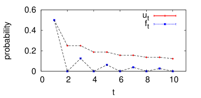
Figure 2: Probability $u_{t}$ to return to the origin, and probability $f_{t}$ for the first return at time $t$. We have fixed the parameter $p$ at $\frac{1}{2}$ to compare the numerical results over $3\times 10^{7}$ random samples (symbols) with the analytic ones (dotted) from Eqs. (16) and (III). Error bars are shown but smaller than the symbol size.

We may furthermore define $f_{t}$ as the probability of the first return to the origin at time $t$ with setting $f_{0}\equiv 0$. It is a standard exercise Grinstead and Snell (1997) to decompose $u_{t>0}$ into

$$u_{t}=f_{0}u_{t}+f_{1}u_{t-1}+\ldots+f_{t}u_{0}=\sum_{\tau=0}^{t}u_{t-\tau}f_{\tau},$$ (17)

according to the first return time. Denoting the generating function for $f_{t}$ as

$$F(x)\equiv\sum_{t=0}^{\infty}f_{t}x^{t},$$ (18)

we may rewrite Eq. (17) as

$$U(x) = 1+\sum_{t=0}^{\infty}\sum_{\tau=0}^{t}u_{t-\tau}f_{\tau}x^{t}$$

$$= 1+\sum_{\tau=0}^{\infty}f_{\tau}x^{\tau}\sum_{t=\tau}^{\infty}u_{t-\tau}x^{t-\tau}$$

$$= 1+F(x)U(x).$$

We thus obtain

$$F(x) = 1-\frac{1}{U(x)}=\frac{\sqrt{1+x}-\sqrt{1-x}}{\sqrt{1+x}+\sqrt{1-x}}$$

$$= \frac{x}{2}+\frac{x^{3}}{8}+\frac{x^{5}}{16}+\frac{5x^{7}}{128}+\frac{7x^{9}}{256}+\ldots,$$

from which one can read off $f_{t}$ at any $t$. Note that $F(x)$ approaches one as $x\rightarrow 1$, which means that this walk is recurrent. Note also that Eq. (III) is an odd function, because the first return after leaving the origin is impossible when $t$ is even. We have checked the expressions for $u_{t}$ and $f_{t}$ with Monte Carlo calculation and drawn the results in Fig. 2.

There is another useful expression for $f_{t}$ written as

$$f_{t}=\frac{[1-(-1)^{t}]\Gamma\left(\frac{t}{2}\right)}{4\sqrt{\pi}~{}\Gamma\left(\frac{t}{2}+\frac{3}{2}\right)},$$ (21)

whereby we can obtain an important quantity $g_{t}$, defined as the number of returns to the origin by time $t$. We decompose $g_{t}$ according to the first return time $\tau$: If the first return time is $\tau$, it means that there must be at least $2^{t}f_{\tau}$ returns among the $2^{t}$ possible trajectories in total. In addition, when those trajectories hit the origin at $\tau$, the number of possibilities should be $2^{\tau}f_{\tau}$, each of which may contain more returning events during the remaining $t-\tau$ time steps. This can be expressed as $2^{\tau}f_{\tau}g_{t-\tau}$ by the definition of $g_{t}$. To sum up, $f_{t}$ and $g_{t}$ are related by

$$g_{t}=\sum_{\tau=1}^{t}\left(f_{\tau}2^{t}+2^{\tau}f_{\tau}g_{t-\tau}\right).$$ (22)

Let us consider the corresponding generating function:

$$G(x) \equiv \sum_{t=0}^{\infty}g_{t}x^{t}=\sum_{t=0}^{\infty}\sum_{\tau=1}^{t}\left(f_{\tau}2^{t}+2^{\tau}f_{\tau}g_{t-\tau}\right)x^{t}$$

$$= \sum_{t=0}^{\infty}(2x)^{t}\sum_{\tau=1}^{t}f_{\tau}+\sum_{t=0}^{\infty}\sum_{\tau=1}^{t}f_{\tau}(2x)^{\tau}\times g_{t-\tau}x^{t-\tau},$$

where the first term can be evaluated by using the general expression in Eq. (21) and the second term can be expressed by convolution as in Eq. (III). After some algebra, we arrive at

$$G(x)=\frac{1-\sqrt{1-4x^{2}}}{2x(1-2x)}+F(2x)G(x),$$ (24)

which yields

$$G(x) = \frac{1-\sqrt{1-4x^{2}}}{2x(1-2x)[1-F(2x)]}$$

$$= x+3x^{2}+8x^{3}+19x^{4}+44x^{5}+\ldots.$$

For example, we find three returning events by time $t=2$, because a trajectory generated by $00$ visits the origin twice and another trajectory from $01$ does it once, while the other two are kept away from the origin. The singular point of $G(x)$ at $x=\frac{1}{2}$ is of particular interest, because $g_{t}\left(\frac{1}{2}\right)^{t}$ corresponds to the average number of returns among all paths by time $t$. Rewriting

$$G(x)=2U^{\prime}(2x)-\frac{1}{2}\left(\frac{1}{1-2x}+\frac{1}{\sqrt{1-4x^{2}}}\right),$$ (26)

where the prime denotes differentiation, we find that the singularity is dominated by the first term on the right-hand side. As a result, if $t=2m+1\gg 1$, the average number of returns scales as

$$\frac{g_{t}}{2^{t}}\sim\frac{m}{2^{2m}}\binom{2m}{m}\sim\sqrt{m},$$ (27)

which is similar to the case of the simple random walk Grinstead and Snell (1997).

IV Conclusion

In summary, we have considered a variant of the persistent random walk and calculated its statistical properties by using the generating-function method. In the limit of $t\rightarrow\infty$, the distribution of the position approaches the Gaussian function, and both the mean and variance are scaled by the factor of $\frac{p}{q}$. We have also obtained the generating functions for return events at $p=q=\frac{1}{2}$ in closed forms. The resulting analytic predictions are fully confirmed by numerical simulation.

Before concluding this work, let us briefly mention how to deal with the periodic boundary condition. We may assume that there are $L$ sites, i.e., $n=1,2,\ldots,L$, with the periodic boundary condition such that $P^{\pm}(n+L,t)=P^{\pm}(n,t)$. The generating function method is made compatible with the boundary condition if we introduce $z_{k}=e^{2\pi ik/L}$ with $k=1,2,\ldots,L$. Then, the following expression

$$\tilde{Q}^{+}(k,t)\equiv\sum_{n=1}^{L}z_{k}^{n}P^{+}(n,t)$$ (28)

corresponds to the discrete Fourier transform of $P^{+}(n,t)$. The inverse transform therefore gives us

$$P^{+}(n,t)=\frac{1}{L}\sum_{k=1}^{L}z_{k}^{-n}\tilde{Q}^{+}(k,t).$$ (29)

We have already obtained the expression $Q^{+}(z,t)$ in Eq. (5) so we need only to use $z_{k}$ instead of $z$ and then plug the resulting $\tilde{Q}^{+}(k,t)$ into Eq. (29). As $t\rightarrow\infty$, only the lowest mode with $k=L$ survives, which corresponds to $z_{k}=1$. Since the conservation of total probability automatically implies $Q^{+}(z=1,t)=1$, we immediately see from Eq. (29) that $P^{+}(n,t\rightarrow\infty)=1/L$, that is, a uniform distribution as indicated by our intuition.