Cross-Points in Domain Decomposition Methods with a Finite Element Discretization

Abstract

Non-overlapping domain decomposition methods necessarily have to exchange Dirichlet and Neumann traces at interfaces in order to be able to converge to the underlying mono-domain solution. Well known such non-overlapping methods are the Dirichlet-Neumann method, the FETI and Neumann-Neumann methods, and optimized Schwarz methods. For all these methods, cross-points in the domain decomposition configuration where more than two subdomains meet do not pose any problem at the continuous level, but care must be taken when the methods are discretized. We show in this paper two possible approaches for the consistent discretization of Neumann conditions at cross-points in a Finite Element setting.

1 Introduction

Domain decomposition methods (DDMs) are among the best parallel solvers for elliptic partial differential equations, see the books [29, 28, 31] and references therein. While classical Schwarz methods only exchange Dirichlet information from subdomain to subdomain, and converge because of overlap, non-overlapping methods like Dirichlet-Neumann, FETI, Neumann-Neumann and optimized Schwarz methods (OSMs) also exchange Neumann traces, or combinations of Dirichlet and Neumann traces between subdomains. In a general decomposition of a domain $\Omega\subset\mathbb{R}^{2}$ into non-overlapping subdomains $(\Omega_{i})_{1\leq i\leq I}$, naturally cross-points arise. Such cross-points, where more than two subdomains meet, do not pose any problem in a continuous variational setting, but as soon as one introduces a finite dimensional approximation, the discretization of a Neumann condition over a cross-point does not follow naturally. The earliest paper dedicated to cross-points dates, to our knowledge, back to 1986: in [8], a Dirichlet-Neumann method is presented for domain decompositions with cartesian topology that can be colored with only two colors. Boundary points, including cross-points, are part of the Neumann subdomains, and all Neumann subdomains are coupled at cross-points, while Dirichlet subdomains are fully decoupled. In [2], a Krylov accelerated DDM to compute the collocation solution of the Poisson equation in a square with Hermite finite elements is studied. There are four subdomains in a $2\times 2$ grid configuration, thus involving a cross-point, and theoretical convergence estimates are provided. The FETI-DP algorithm [9, 24] modifies the FETI algorithm [27] at cross-points by replacing the dual variables by primal ones and thus avoiding the problem of Neumann conditions there. Similarly, strong coupling at cross-points is also proposed in [1, 3] for nodal finite elements. In [13], it was shown for optimized Schwarz methods (OSMs) in an algebraic setting that optimized Robin parameters scale differently at cross-points, namely like $O(1/h)$, in contrast to $O(1/\sqrt{h})$ at interface points which are not cross-points, see also [26] for condition number estimates in the presence of cross-points. Cross points can also be handled in the context of mortar methods, and in very special symmetric configurations, it is actually possible for cross-points not to pose any problems, see [14]. The cross-point problem can be avoided entirely when using cell-centered finite volume discretizations, because they do not contain cross-points at the discrete level, see [4] for the convergence of the cell-centered finite volume Optimized Schwarz method with Robin transmission conditions; see [18] for the convergence of the cell-centered finite volume Optimized Schwarz with Ventcell transmission conditions in the absence of cross-points; and [15] for the extension of the convergence proof to symmetric positive definite transmission operators even in the presence of cross-points.

We describe in this paper in detail two approaches to exchange Neumann traces over cross points in a finite element setting for two dimensional problems: the auxiliary variable method, and complete communication. The auxiliary variable method keeps in addition to the primal unknowns also auxiliary unknowns representing interface data in each subdomain. These auxiliary variables permit a consistent discretization of the Neumann traces at cross points while only communicating with neighboring domains sharing a boundary of non-zero one-dimensional measure. As a first main result, we show that with auxiliary variables, one can prove convergence of the discretized domain decomposition algorithm using energy estimates, which is not possible for finite element discretizations with cross-points otherwise [14]. A disadvantage of the auxiliary variables is that they are not necessarily converging to a limit, but this does not affect the convergence of the primal unknowns in the iteration. The complete communication method needs to exchange information with all subdomains touching at cross points, also those which touch only at a point, in order to have a consistent discretization of Neumann conditions. Our second main result is to show how to determine among the many possible splittings of Neumann traces one that minimizes oscillation.

Our paper is organized as follows: in §2, we describe on the concrete example of an OSM why the discretization of the Neumann part of the transmission condition is ambiguous at cross-points. In §3, we present the first approach on how to transmit Neumann information near cross-points using auxiliary variables, and give a general convergence proof for a non-overlapping OSM discretized by finite elements with cross-points. In §4, we describe how Neumann information can be transmitted near cross-points by communicating among all subdomains sharing the cross point, and we propose a specific method minimizing oscillation. After our conclusions in §5, we show in Appendix A that instead of using higher order, so called Ventcell transmission conditions, see for example [20, 21, 5, 22, 23, 11, 10], one can algebraically naturally obtain such conditions from Robin conditions using mass lumping techniques in a finite element setting. This avoids the need for discretizing higher order differential operators in the tangential direction, and even works at cross-points, which is our third important result.

2 The discrete Optimized Schwarz Method

For the elliptic problem $\mathcal{L}u=f$ in $\Omega$, and a non-overlapping decomposition $(\Omega_{i})_{1\leq i\leq I}$, the OSM with Robin transmission conditions at the continuous level is (see for example [10])

Algorithm 2.1 (OSM).

1. Set $p>0$.

2. Start with an initial guess $u_{i}^{0}$ in each subdomain $\Omega_{i}$.

3. Until convergence, compute in parallel the unique solution $u_{i}^{n+1}$ to

   $$\mathcal{L}u_{i}^{n+1} = f\;\text{in $\Omega_{i}$},$$ (1)

   $$\frac{\partial u^{n+1}_{i}}{\partial\bm{n}_{ii^{\prime}}}+pu^{n+1}_{i} = \frac{\partial u^{n}_{i^{\prime}}}{\partial\bm{n}_{ii^{\prime}}}+pu^{n}_{i^{\prime}}\;\text{on $\partial\Omega_{i}\cap\partial\Omega_{i^{\prime}}$}.$$ (2)

In a variational formulation of Algorithm 2.1, cross-points do not pose any problems, since they have measure zero. In a finite dimensional approximation however, using for example finite elements, the Neumann part of the Robin transmission conditions is only known as a variational quantity, as an integral over the edges connected to the cross-point. When discretizing OSM (or any DDM), there are two guiding principles:

1. The discrete mono-domain solution should be a fixed point of the discrete OSM.

2. The discrete OSM should have a unique fixed point.

We show in this section that it is not completely straightforward to follow these two principles when cross-points are present.

2.1 Geometric setting and notation

Let $\mathcal{T}$ be a polygonal mesh of $\Omega\subset\mathbb{R}^{2}$. Let $(\Omega_{i})_{1\leq i\leq I}$ be a non-overlapping domain decomposition of the domain $\Omega$. We assume that the subdomains $\Omega_{i}$ are polygonal, and that each cell of $\mathcal{T}$ is included in exactly one subdomain. Let $\mathcal{T}_{i}$ be the restriction of the mesh $\mathcal{T}$ to $\Omega_{i}$, and denote by $\bm{x}_{j}$ the vertices of the mesh $\mathcal{T}$. We consider a finite element space $\mathcal{P}(\mathcal{T})$ subset of $H_{0}^{1}(\Omega)$ with the following properties:

1. There is exactly one degree of freedom at each vertex of $\mathcal{T}$ for $\mathcal{P}(\mathcal{T})$.

2. For any edge $[\bm{x}_{j}\bm{x}_{j^{\prime}}]$ of $\mathcal{P}(\mathcal{T})$ and for any $u$ in $\mathcal{P}(\mathcal{T})$, $u(\bm{x}_{j})=0$ and $u(\bm{x}_{j^{\prime}})=0$ implies $u$ vanishes on the entire edge $[\bm{x}_{j}\bm{x}_{j^{\prime}}]$.

Both these conditions are satisfied for $P_{1}$ elements on triangular meshes and $Q_{1}$ elements on cartesian ones. We define $\mathcal{P}(\mathcal{T}_{i}):=\{u_{|\Omega_{i}}|u\in\mathcal{P}(\mathcal{T})\}$. We denote the hat functions by $\phi_{j}$, i.e. the unique function in $\mathcal{P}(\mathcal{T})$ such that

$$\phi_{j}(\bm{x}_{j^{\prime}})=\begin{cases}1&\text{if $j=j^{\prime}$,}\\ 0&\text{if $j\neq j^{\prime}$,}\end{cases}$$

and by $\phi_{i;j}$ we denote $(\phi_{j})_{|\Omega_{i}}$. We will systematically use for subdomain indices the letter $i$, and separate it from nodal indices $j$ using a semicolon. The discretized OSM operates then on the space

$$V:=\bigotimes_{i=1}^{N}\mathcal{P}(\mathcal{T}_{i}).$$

Since a node located on a subdomain boundary may belong to more than one subdomain, we use the index $i$ in $\bm{x}_{i;j}$ to distinguish degrees of freedom located at the same node but belonging to different subdomains.

2.2 Discretization of Robin transmission conditions

The discrete Neumann boundary condition must be computed variationally in a FEM setting, see for example [31, p.3, Eq. (1.7)]. Near cross-points, the Neumann boundary condition is like an integral over both edges that are adjacent to the cross-point and belonging to the boundary of the subdomain. As there is no canonical way to split that variational Neumann boundary condition, it is not clear how we should split that quantity when it comes to transmitting Neumann information between adjacent subdomains near cross points. Any splitting should satisfy the two guiding principles listed at the beginning of §2.

To investigate this problem, it suffices to study the case of the elliptic operator $\mathcal{L}:=\eta-\operatorname{\triangle}$, $\eta>0$ in Algorithm 2.1. Following finite element principles, we should solve for every subdomain $\Omega_{i}$ at every new iteration $n+1$

$$\eta\int_{\Omega_{i}}u_{i}^{n+1}\phi_{i;j}+\int_{\Omega_{i}}\nabla u_{i}^{n+1}\cdot\nabla\phi_{i;j}+p\int_{\partial\Omega_{i}}u_{i}^{n+1}\phi_{i;j}\mathrm{d}\sigma(\bm{x})=f_{i;j}+g_{i;j}^{n+1}$$ (3)

for all $j$ such that $\bm{x}_{i;j}$ is a node of mesh $\mathcal{T}$ located in $\overline{\Omega}_{i}$, in order to find the new finite element subdomain solution approximation $u_{i}^{n+1}=\sum_{j}u_{i;j}^{n+1}\phi_{i;j}$. The data $g_{i;j}^{n+1}$ needs to be gathered from neighboring subdomains, satisfying (2) variationally. We denote by the matrix $\mathbf{A}_{i}$ the sum of the mass and stiffness contributions corresponding to the interior equation $\eta-\operatorname{\triangle}$ in each subdomain $\Omega_{i}$,

$$A_{i;j,j^{\prime}}:=\eta\int_{\Omega_{i}}\phi_{i;j}(\bm{x})\phi_{i;j^{\prime}}(\bm{x})\mathrm{d}\bm{x}+\int_{\Omega_{i}}\nabla\phi_{i;j}(\bm{x})\nabla\phi_{i;j^{\prime}}(\bm{x})\mathrm{d}\bm{x}.$$ (4)

The matrix $\mathbf{B}_{i}^{\textrm{cons}}$ contains the boundary contribution $p\int_{\partial\Omega_{i}}u_{i}^{n+1}\phi_{i;j}\mathrm{d}\sigma(\bm{x})$, including the Robin parameter $p$: if the finite elements are linear on each edge, which holds for $Q_{1}$ and $P_{1}$ elements, we have the consistent interface mass matrix

$$B^{\textrm{cons}}_{i;j,j^{\prime}}:=\begin{cases}\frac{p}{3}\sum_{j^{\prime\prime}}\lvert\bm{x}_{i;j}-\bm{x}_{i;j^{\prime\prime}}\rvert&\text{if $j^{\prime}=j$ and $\bm{x}_{i;j}$ lies on $\partial\Omega_{i}$},\\ \frac{p}{6}\lvert\bm{x}_{i;j}-\bm{x}_{i;j^{\prime}}\rvert&\text{if $[\bm{x}_{i;j}\bm{x}_{i;j^{\prime}}]$ is an edge of $\partial\Omega_{i}$},\\ 0&\text{otherwise},\end{cases}$$ (5)

where the sum is taken over all $j^{\prime\prime}\neq j$ such that $[\bm{x}_{j}\bm{x}_{j^{\prime\prime}}]$ is a boundary edge of $\mathcal{T}_{i}$. A lumped version of the interface mass matrix $\mathbf{B}_{i}^{\textrm{cons}}$ is

$$B^{\textrm{lump}}_{i;j,j^{\prime}}:=\begin{cases}\frac{p}{2}\sum_{j^{\prime\prime}}\lvert\bm{x}_{i;j}-\bm{x}_{i;j^{\prime\prime}}\rvert&\text{if $j=j^{\prime}$ and $\bm{x}_{i;j}$ lies on $\partial\Omega_{i}$},\\ 0&\text{otherwise},\end{cases}$$ (6)

where again the sum is taken over all $j^{\prime\prime}\neq j$ such that $[\bm{x}_{j}\bm{x}_{j^{\prime\prime}}]$ is a boundary edge of $\mathcal{T}_{i}$. We explain in Appendix A why using a lumped interface mass matrix $\mathbf{B}^{\textrm{lump}}_{i}$ leads to faster convergence than using a consistent mass matrix $\mathbf{B}_{i}$, by interpreting the lumping process at the continuous level as introducing a higher order term in the transmission condition, see also [7]. This higher order term can even be optimized using a new concept of overlumping we will introduce. Note that in the context of discrete duality finite volume methods, it was shown in [12] that the consistent mass matrix can even completely destroy the asymptotic performance of the optimized Schwarz method, even without cross-points. This is however not the case for the finite element discretizations we consider here.

Using the matrix notation we introduced, we have to solve at each Schwarz iteration the to (3) equivalent matrix problem

$$(\mathbf{A}_{i}+\mathbf{B}^{\textrm{lump}}_{i})\bm{u}_{i}^{n+1}=\bm{f}_{i}+\bm{g}^{n+1}_{i},$$ (7)

where the vector $\bm{g}^{n+1}_{i}$ is zero at interior nodes of $\Omega_{i}$ and contains the values $\bm{g}_{i,i^{\prime}}^{n}$ transmitted from the neighboring subdomains $\Omega_{i^{\prime}}$ on the interface nodes of $\Omega_{i}$. The computation of $\bm{f}_{i}$ and $\bm{g}^{n+1}_{i}$ should be done in such a way that the two guiding principles listed at the beginning of §2 are satisfied. At the continuous level, $\bm{f}_{i}$ would just be the restriction of $f$ to $\Omega_{i}$, and hence, if the continuous function $f$ is known, one can set

$$f_{i;j}:=\int_{\Omega_{i}}f(\bm{x})\phi_{i;j}\mathrm{d}\bm{x}.$$

If only $\bm{f}$ is known, then one has to choose $\bm{f}_{i}$ in such a way that the $j$th component of $\bm{f}$ satisfies $f_{j}=\sum_{i}f_{i;j}$ where the sum happens over all indices $i$ such that $\bm{x}_{j}$ belongs to $\overline{\Omega}_{i}$. For the transmitted values $\bm{g}^{n}_{i,i^{\prime}}$ with a finite element discretization, the Neumann contribution is defined by a variational problem. At the continuous level, if $(\eta-\operatorname{\triangle})u_{i}=f$ inside $\Omega_{i}$, we have by Green’s formula

$$\int_{\partial\Omega_{i}}\frac{\partial u_{i}}{\partial\bm{n}_{i}}v=\eta\int_{\Omega_{i}}uv+\int_{\Omega_{i}}\nabla u\nabla v-\int_{\Omega_{i}}fv.$$ (8)

This formula can be used to define discrete Neumann boundary conditions: for $\bm{x}_{i;j}$ a vertex of the fine mesh located on $\partial\Omega_{i}$, we define

$$\mathcal{N}_{i;j}(u_{i}):=\eta\int_{\Omega_{i}}u_{i}\phi_{i;j}+\int_{\Omega_{i}}\nabla u_{i}\nabla\phi_{i;j}-\bm{f}_{i;j}.$$ (9)

At the discrete level, the no Neumann jump condition satisfied by the discrete mono-domain solution is given by $\sum_{i}\mathcal{N}_{i;j}(u_{i})=0$ where the sum is over all $i$ such that $\bm{x}_{j}$ is a boundary vertex of $\mathcal{T}_{i}$. For interface points that belong to exactly two subdomains $\overline{\Omega}_{i}$ and $\overline{\Omega}_{i^{\prime}}$, the Robin update is not ambiguous and we set

$$g^{n}_{i,i^{\prime};j}:=-\mathcal{N}_{i^{\prime};j}(u^{n}_{i^{\prime}})+\frac{p}{2}u_{i^{\prime};j}^{n}\sum_{j^{\prime}}\lvert\bm{x}_{i;j}-\bm{x}_{i;j^{\prime}}\rvert,$$ (10)

where the sum is over all $j^{\prime}$ such that $[\bm{x}_{j}\bm{x}_{j^{\prime}}]$ is a boundary edge of both $\mathcal{T}_{i}$ and $\mathcal{T}_{i^{\prime}}$. The $g^{n}_{i,i^{\prime};j}$ must be sent by subdomain $\Omega_{i^{\prime}}$ to subdomain $\Omega_{i}$, and then $g^{n+1}_{i;j}=g^{n}_{i,i^{\prime};j}$, since there is only one contribution from the unique neighbor $\Omega_{i^{\prime}}$.

2.3 Ambiguity of the Robin update at cross-points

To see why the Robin update (10) can not be used at cross points, consider as an example the cross point $\bm{x}_{1}$ belonging to subdomain $\Omega_{1}$ shown in Figure 1.

Figure 1: Example of a cross point in the decomposition

Following (10), to compute $\bm{g}^{n+1}_{1}$ at cross-point $\bm{x}_{1}$, one would intuitively set

$$\begin{split}g^{n+1}_{1;1}&=-\mathcal{N}_{2;13}(u^{n}_{2})+\frac{p}{2}\lvert\bm{x}_{1}-\bm{x}_{3}\rvert u_{2;1}^{n}\\ &\phantom{=}-\mathcal{N}_{5;12}(u^{n}_{5})+\frac{p}{2}\lvert\bm{x}_{1}-\bm{x}_{2}\rvert u_{5;1}^{n},\end{split}$$

where $\mathcal{N}_{2;13}$ is the part of $\mathcal{N}_{2}$ located on edge $[\bm{x}_{1}\bm{x}_{3}]$, and likewise for $\mathcal{N}_{5;12}$. Unfortunately, at the discrete level, the Neumann contributions of $u^{n}_{2}$ and $u^{n}_{5}$ at $\bm{x}_{1}$ are only known as an integral over the edges coming from $\bm{x}_{1}$. We cannot distinguish the contribution of each edge to the Neumann conditions $\mathcal{N}_{2}(u^{n}_{2})$ and $\mathcal{N}_{5}(u^{n}_{5})$. We only know that

$$\mathcal{N}_{2}(u^{n}_{2})=\mathcal{N}_{2;13}(u^{n}_{2})+\mathcal{N}_{2;14}(u^{n}_{2}),\quad\mathcal{N}_{5}(u^{n}_{5})=\mathcal{N}_{5;12}(u^{n}_{5})+\mathcal{N}_{5;16}(u^{n}_{5}).$$

When transmitting the Robin condition at a cross point, the Neumann contribution must be split across each edge in such a way that the discrete mono-domain solution remains a fixed point of the optimized Schwarz method, see principle 1 at the beginning of §2. The discrete mono-domain solution satisfies

$$u_{i;j}=u_{i^{\prime};j}\quad\text{for all $i^{\prime}$ with $\bm{x}_{j}$ in $\Omega_{i^{\prime}}$, and}\quad\sum_{i,\bm{x}_{j}\in\partial\Omega_{i}}\mathcal{N}_{i;j}(u_{i})=0.$$ (11)

We should therefore split the Neumann contributions in such a way that if properties (11) are satisfied for an iterate $u_{i}^{n}$, then the transmission conditions do not change any more, $g_{i;j}^{n+1}=g_{i;j}^{n}$. We show in the next two sections that such a splitting can either be obtained using auxiliary variables and communicating only with neighbors, or by communicating with all subdomains that share the cross-point.

3 Auxiliary variables at cross-points

We now show how to introduce auxiliary variables near the cross points. At the continuous level, we have on the interface between subdomain $\Omega_{i}$ and $\Omega_{i^{\prime}}$ from (2) the identity

$$g^{n+1}_{i}=\frac{\partial u^{n+1}_{i}}{\partial\bm{n}_{ii^{\prime}}}+pu^{n+1}_{i}=\frac{\partial u^{n}_{i^{\prime}}}{\partial\bm{n}_{ii^{\prime}}}+pu^{n}_{i^{\prime}}=-\frac{\partial u^{n}_{i^{\prime}}}{\partial\bm{n}_{i^{\prime}i}}+pu^{n}_{i^{\prime}}=-g^{n}_{i^{\prime}}+2pu^{n}_{i^{\prime}},$$

since by definition $g^{n}_{i^{\prime}}=\frac{\partial u^{n}_{i^{\prime}}}{\partial\bm{n}_{i^{\prime}i}}+pu^{n}_{i^{\prime}}$ and the normals are in opposite directions. At the discrete level, the same equality can be used to update the Robin transmission conditions,

$$g^{n+1}_{i;j}=-g^{n}_{i^{\prime};j}+2\frac{p}{2}u_{i^{\prime};j}^{n}\sum_{j^{\prime}}\lvert\bm{x}_{i;j}-\bm{x}_{i;j^{\prime}}\rvert,$$ (12)

where the sum is over all $j^{\prime}$ such that $[\bm{x}_{j}\bm{x}_{j}^{\prime}]$ is a boundary edge of $\mathcal{T}_{i}$. This is very useful in practice, because one then does not even need to implement a normal derivative evaluation [16]. At interface points which are not cross-points, this update will give the same update as applying formula (10) using the definition (9). Therefore, if we are given the values $g_{i,i^{\prime};j}^{n}$ which represent the Robin transmission information sent from subdomain $i^{\prime}$ to subdomain $i$, we can compute $u^{n+1}_{i}$ by setting

$$g_{i;j}^{n+1}=\sum_{i^{\prime}}g_{i,i^{\prime};j}^{n}$$ (13)

and solving Eq (7). The sum in (13) above is over all $i^{\prime}$ such that there exists an edge originating from the vertex $\bm{x}_{j}$ that belongs to both $\mathcal{T}_{i}$ and $\mathcal{T}_{i^{\prime}}$. We then set

$$g^{n+1}_{i^{\prime},i;j}:=-g^{n}_{i,i^{\prime};j}+2\frac{p}{2}u_{i;j}^{n+1}\sum_{j^{\prime}}\lvert\bm{x}_{i;j}-\bm{x}_{i;j^{\prime}}\rvert,$$ (14)

where the sum is over all $j^{\prime}$ such that $[\bm{x}_{j}\bm{x}_{j^{\prime}}]$ is a boundary edge of both $\mathcal{T}_{i}$ and $\mathcal{T}_{i^{\prime}}$. For this we need however to store the auxiliary variables $g^{n+1}_{i^{\prime},i;j}$, because it is not possible to recover $g^{n+1}_{i^{\prime},i;j}$ from $u_{i}^{n+1}$ when $\bm{x}_{j}$ is a cross-point. Only the sum over $i^{\prime}$ of the $g^{n+1}_{i^{\prime},i;j}$ can be recovered from $u_{i}^{n+1}$.

Since the $g^{n}_{i,i^{\prime};j}$ represent a split of the discrete Robin conditions, we can deduce from them a split of the discrete Neumann conditions and introduce the $\mathcal{N}_{i^{\prime},i;j}^{n}$. We set

$$\mathcal{N}_{i,i^{\prime};j}^{n+1}:=g^{n}_{i,i^{\prime};j}-\frac{p}{2}\left(\sum_{j^{\prime}}\lvert\bm{x}_{j}-\bm{x}_{j^{\prime}}\rvert\right)u_{i;j}^{n+1},$$ (15)

where the sum is over all $j^{\prime}$ such that $[\bm{x}_{j}\bm{x}_{j^{\prime}}]$ is a boundary edge of both $\mathcal{T}_{i}$ and $\mathcal{T}_{i^{\prime}}$. By Eqs. (6), (9) and (7), we obtain

$$\mathcal{N}_{i;j}(u_{i}^{n+1})=\sum_{i^{\prime}}\mathcal{N}_{i,i^{\prime};j}^{n+1},$$ (16)

where the sum is over all $i^{\prime}$ such that there exists an edge originating from $\bm{x}_{j}$ that is a boundary edge of both $\mathcal{T}_{i}$ and $\mathcal{T}_{i^{\prime}}$.

3.1 Convergence of the auxiliary variable method

At the continuous level, one can prove convergence of OSM using energy estimates, see for example [25, 6]. At the discrete level, this technique fails in general [14], precisely because of the cross-points.

We prove now convergence of OSM in the presence of cross-points, when auxiliary variables are used.

Lemma 3.1.

Let $\bm{f}=(f_{j})$ be a right hand side of the discretized operator $\eta-\operatorname{\triangle}$ with $f_{i;j}$ such that $\sum_{i}f_{i;j}=f_{j}$. Then there exist $g_{i,i^{\prime};j}$ which are a fixed point of the discrete Optimized Schwarz algorithm with auxiliary variables near cross points.

Proof.

Let $\bm{u}$ be the discrete mono-domain solution. Let $\bm{u}_{i}$ be the restriction of $\bm{u}$ to $\mathcal{T}_{i}$. Let

$$\mathcal{E}_{i;j} :=\{j^{\prime\prime},[\bm{x}_{j}\bm{x}_{j^{\prime\prime}}]\text{ boundary edge of $\mathcal{T}_{i}$}\},$$

$$\mathcal{E}_{i;i^{\prime};j} :=\{j^{\prime\prime},[\bm{x}_{j}\bm{x}_{j^{\prime\prime}}]\text{ boundary edge of $\mathcal{T}_{i}$ and of $\mathcal{T}_{i^{\prime}}$ }\}.$$

We use formula (9) to obtain the existence of $g_{i;j}$ such that the solution of (7) are the $\bm{u}_{i}$. For any given cross-point node $\bm{x}_{j}$, we have to split the $g_{i;j}$ into $g_{i,i^{\prime};j}$ that satisfy

$$g_{i;j} =\sum_{i^{\prime}\;\text{s.t.}\;\mathcal{E}_{i;i^{\prime};j}\neq\emptyset}g_{i,i^{\prime};j},$$

$$g_{i^{\prime},i;j} =-g_{i,i^{\prime};j}+2\frac{p}{2}u_{j}\sum_{j^{\prime}\in\mathcal{E}_{i;i^{\prime};j}}\lvert\bm{x}_{i,j}-\bm{x}_{i,j^{\prime}}\rvert.$$

Subtracting the Dirichlet parts on both sides in the first equation, and transferring half the Dirichlet part in the second equation from the right to the left, we get

$$g_{i;j}-\frac{p}{2}u_{j}\sum_{j^{\prime\prime}\in\mathcal{E}_{i;j}}\lvert\bm{x}_{i,j}-\bm{x}_{i,j^{\prime}}\rvert =\sum_{i^{\prime}\;\text{s.t.}\;\mathcal{E}_{i;i^{\prime};j}\neq\emptyset}(g_{i,i^{\prime};j}-\frac{p}{2}u_{j}\sum_{j^{\prime\prime}\in\mathcal{E}_{i,i^{\prime};j}}\lvert\bm{x}_{i,j}-\bm{x}_{i,j^{\prime}}\rvert),$$

$$g_{i^{\prime},i;j}-\frac{p}{2}u_{j}\sum_{j^{\prime\prime}\in\mathcal{E}_{i,i^{\prime};j}}\lvert\bm{x}_{i,i^{\prime},j}-\bm{x}_{i,j^{\prime}}\rvert =-(g_{i,i^{\prime};j}-\frac{p}{2}u_{j}\sum_{j^{\prime\prime}\in\mathcal{E}_{i,i^{\prime};j}}\lvert\bm{x}_{i,j}-\bm{x}_{i,j^{\prime}}\rvert),$$

We recognize the discrete Neumann conditions, see (15). So the problem becomes the concrete splitting problem of Neumann conditions: given $\mathcal{N}_{i;j}$, find $\mathcal{N}_{i,i^{\prime};j}$ such that

$$\mathcal{N}_{i;j} =\sum_{i^{\prime}\;\text{s.t.}\;\mathcal{E}_{i;i^{\prime};j}\neq\emptyset}\mathcal{N}_{i,i^{\prime};j},$$ (17)

$$\mathcal{N}_{i,i^{\prime};j} =-\mathcal{N}_{i^{\prime},i;j}.$$ (18)

By (11), since $\bm{u}$ is the discrete mono-domain solution, we have $\sum_{i}\mathcal{N}_{i;j}=0$. For each cross-point $\bm{x}_{j}$, we define a graph $G$, whose set of vertices $V(G)$ and set of edges $E(G)$ are defined as

$$V(G) =\{i,\;\bm{x}_{j}\in\Omega_{i}\},$$

$$E(G) =\{\{i,i^{\prime}\}\subset V(G),\;\text{$\mathcal{T}_{i}$ and $\mathcal{T}_{i^{\prime}}$ share an edge originating from $\bm{x}_{j}$}\}.$$

We apply now Lemma B.1 to conclude the proof. ∎

Theorem 3.2.

The optimized Schwarz method (2.1) discretized with finite elements (3) and using auxiliary variables for the transmission conditions is convergent.

Proof.

Because of Lemma 3.1, we can assume without loss of generality that $\bm{f}_{i}=0$. For each subdomain $\Omega_{i}$, we multiply the definition of the discrete Neumann condition (9) by $u_{i;j}$, then sum over all $j$ such that $\bm{x}_{j}$ belongs to $\overline{\Omega}_{i}$ to obtain

$$\begin{split}\int_{\Omega_{i}}\lvert\nabla u_{i}^{n+1}\rvert^{2}&+\eta\int_{\Omega_{i}}\lvert u_{i}^{n+1}\rvert^{2}\\ &=\sum_{\bm{x}_{j}\in\partial\Omega_{i}}\mathcal{N}_{i;j}^{n+1}u_{i;j}^{n+1}.\\ &=\sum_{i^{\prime}}\sum_{\bm{x}_{j}\in\partial\Omega_{i}\cap\partial\Omega_{i^{\prime}}}\mathcal{N}_{i,i^{\prime};j}^{n+1}u_{i;j}^{n+1}\qquad\text{(by\leavevmode\nobreak\ \eqref{eq:sumNeumann})}\\ &=\sum_{i^{\prime}}\sum_{\bm{x}_{j}\in\partial\Omega_{i}\cap\partial\Omega_{i^{\prime}}}\frac{\lvert\mathcal{N}_{i,i^{\prime};j}^{n+1}+\frac{p}{2}\sum_{j^{\prime\prime}}\lvert\bm{x}_{j}-\bm{x}_{j^{\prime\prime}}\rvert u_{i;j}^{n+1}\rvert^{2}}{2p\sum_{j^{\prime\prime}}\lvert\bm{x}_{j}-\bm{x}_{j^{\prime\prime}}\rvert}\\ &\phantom{=\sum_{i^{\prime}}\sum_{\bm{x}_{j}\in\partial\Omega_{i}\cap\partial\Omega_{i^{\prime}}}}-\frac{\lvert\mathcal{N}_{i,i^{\prime};j}^{n+1}-\frac{p}{2}\sum_{j^{\prime\prime}}\lvert\bm{x}_{j}-\bm{x}_{j^{\prime\prime}}\rvert u_{i;j}^{n+1}\rvert^{2}}{2p\sum_{j^{\prime\prime}}\lvert\bm{x}_{j}-\bm{x}_{j^{\prime\prime}}\rvert},\\ &=\sum_{i^{\prime}}\sum_{\bm{x}_{j}\in\partial\Omega_{i}\cap\partial\Omega_{i^{\prime}}}\frac{\lvert g_{i,i^{\prime};j}^{n}\rvert^{2}-\lvert g_{i^{\prime},i;j}^{n+1}\rvert^{2}}{2p\sum_{j^{\prime\prime}}\lvert\bm{x}_{j}-\bm{x}_{j^{\prime\prime}}\rvert}\qquad\text{(by\leavevmode\nobreak\ \eqref{eq:defN} and\leavevmode\nobreak\ \eqref{eq:RobinUpdateAuxiliary})}.\end{split}$$

We now sum over all subdomains $i$ and over the iteration index $n$ to get

$$\begin{split}\sum_{n=0}^{N}\sum_{i=1}^{I}\int_{\Omega_{i}}\lvert\nabla u_{i}^{n+1}\rvert^{2}+\eta\int_{\Omega_{i}}\lvert u_{i}^{n+1}\rvert^{2}&=\sum_{i,i^{\prime}}\sum_{\bm{x}_{j}\in\partial\Omega_{i}\cap\partial\Omega_{i^{\prime}}}\frac{\lvert g_{i,i^{\prime};j}^{0}\rvert^{2}-\lvert g_{i^{\prime},i;j}^{N+1}\rvert^{2}}{2p\sum_{j^{\prime\prime}}\lvert\bm{x}_{j}-\bm{x}_{j^{\prime\prime}}\rvert}\\ &\leq\sum_{i,i^{\prime}}\sum_{\bm{x}_{j}\in\partial\Omega_{i}\cap\partial\Omega_{i^{\prime}}}\frac{\lvert g_{i,i^{\prime};j}^{0}\rvert^{2}}{2p\sum_{j^{\prime\prime}}\lvert\bm{x}_{j}-\bm{x}_{j^{\prime\prime}}\rvert}.\end{split}$$

This shows that the sum over the energy over all iterates and subdomains stays bounded, as the iteration number $N$ goes to infinity, which implies that the energy of the iterates, and hence the iterates converge to zero. ∎

3.2 Numerical observation using auxiliary variables

Using auxiliary variables can have surprising numerical side effects. We show in Figure 2

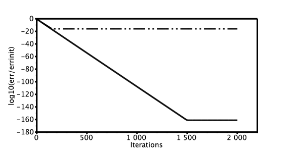
Figure 2: Error using OSM with auxiliary variables for $4\times 1$ (solid) and $2\times 2$ (dashed-dotted) subdomains

the error measured in $L^{\infty}$ of OSM with auxiliary variables for the domain $\Omega=(0,4)^{2}$ decomposed once into $2\times 2$ subdomains and once into $4\times 1$ subdomains, for $p=2.0$ and $\eta=0.0$ and mesh size $h=1/10$. We iterate directly on the error equations, $f=0$, and initialize the transmission conditions with random values. We observe that in the presence of cross points, convergence stagnates around the machine precision, whereas without, the stagnation comes much later.

To understand these results, we need to consider floating point arithmetic, see [19, 30, 17], and in particular the machine precision macheps and the smallest positive floating point number minreal. We used in the above experiment double precision in C++ so macheps$=2^{-53}\approx 1.1\cdot^{-16}$ and minreal$\approx 4.9\cdot 10^{-324}$. Had we been computing a real problem with nonzero right hand side $f$, we would expect stagnation near the machine precision. However, when iterating directly on the errors, stagnation should occur much later, at the level of the smallest positive floating point number.

To analyze the early stagnation observed, we consider a simple model problem with $2\times 2$ subdomains, see Figure 3,

Figure 3: Degenerate case.

where there is exactly one $Q_{1}$ element per subdomain and the only interior node is a cross-point. This means the mono-domain solutions $u$ is a scalar. We thus have $\Omega=(-h,h)\times(-h,h)$, and for the subdomains $\Omega_{1}=(0,h)\times(0,h)$, $\Omega_{2}=(-h,0)\times(0,h)$, $\Omega_{3}=(-h,0)\times(-h,0)$, $\Omega_{4}=(0,h)\times(-h,0)$. We apply the OSM with lumped Robin transmission conditions and $f=0$. Since there is only one interior node in the whole mesh, there is only a single test function $\phi$ with $\phi(x,y)=(1-\lvert x\rvert)(1-\lvert y\rvert)$. By Eq. (7), we have

$$\begin{split}A_{1}=A_{2}=A_{3}=A_{4}&=\eta h^{2}\left(\int_{0}^{1}(1-x)^{2}\mathrm{d}x\right)^{2}+\int_{0}^{1}(1-x)^{2}\mathrm{d}x+\int_{0}^{1}(1-y)^{2}\mathrm{d}y\\ &=\frac{\eta h^{2}}{9}+\frac{2}{3}.\end{split}$$

We use lumped Robin transmission conditions, and by (6), we get

$$B_{1}=B_{2}=B_{3}=B_{4}=\frac{p}{2}h\left(\int_{0}^{1}(1-x)\mathrm{d}x+\int_{0}^{1}(1-y)\mathrm{d}y\right)=ph.$$

Therefore, we have by (7) and (13)

$$u_{i}^{n+1}=\frac{g_{i}^{n+1}}{\frac{2}{3}+\frac{\eta h^{2}}{9}+ph},\quad\text{$i=1,\ldots,4$}.$$

Thus, for the OSM iteration, we obtain

$$u_{1}^{n+1} =\frac{g_{12}^{n}+g_{14}^{n}}{\frac{2}{3}+\frac{\eta h^{2}}{9}+ph}, u_{2}^{n+1} =\frac{g_{23}^{n}+g_{21}^{n}}{\frac{2}{3}+\frac{\eta h^{2}}{9}+ph},$$ (19)

$$u_{3}^{n+1} =\frac{g_{32}^{n}+g_{34}^{n}}{\frac{2}{3}+\frac{\eta h^{2}}{9}+ph}, u_{4}^{n+1} =\frac{g_{43}^{n}+g_{41}^{n}}{\frac{2}{3}+\frac{\eta h^{2}}{9}+ph},$$

and by (14), we get

$$g^{n+1}_{i^{\prime},i}:=-g^{n}_{i,i^{\prime}}+phu_{i}^{n+1}.$$

Eliminating the $u_{i}^{n+1}$ from the iteration leads to

$$\begin{bmatrix}g_{1,2}^{n+1}\\ g_{2,1}^{n+1}\\ g_{2,3}^{n+1}\\ g_{3,2}^{n+1}\\ g_{3,4}^{n+1}\\ g_{4,3}^{n+1}\\ g_{4,1}^{n+1}\\ g_{1,4}^{n+1}\end{bmatrix}=\begin{bmatrix}0&\alpha-1&\alpha&0&0&0&0&0\\ \alpha-1&0&0&0&0&0&0&\alpha\\ 0&0&0&\alpha-1&\alpha&0&0&0\\ 0&\alpha&\alpha-1&0&0&0&0&0\\ 0&0&0&0&0&\alpha-1&\alpha&0\\ 0&0&0&\alpha&\alpha-1&0&0&0\\ \alpha&0&0&0&0&0&0&\alpha-1\\ 0&0&0&0&0&\alpha&\alpha-1&0\end{bmatrix}\begin{bmatrix}g_{1,2}^{n}\\ g_{2,1}^{n}\\ g_{2,3}^{n}\\ g_{3,2}^{n}\\ g_{3,4}^{n}\\ g_{4,3}^{n}\\ g_{4,1}^{n}\\ g_{1,4}^{n},\end{bmatrix},$$

where we introduced the scalar quantity

$$\alpha=\frac{ph}{\frac{\eta h^{2}}{9}+\frac{2}{3}+ph}.$$

Since $0<\alpha<1$, the $\ell^{\infty}$ norm of this iteration matrix is $1$, and hence its spectral radius is bounded by $1$. Note however that $1$ and $-1$ are eigenvalues of this matrix, with corresponding eigenvectors

$$(-1,1,-1,1,-1,1,-1,1)^{T}\quad\mbox{and}\quad(1,1,-1,-1,1,1,-1,-1)^{T}.$$

This shows that the vector of auxiliary variables will not converge to $0$ in general. However, the modes with eigenvalue $+1$ and $-1$ make no contribution to the $u_{i}$, see Eq. (19), so the algorithm will converge for the $u_{i}^{n}$, as proved in Theorem 3.2. In floating point arithmetic however, the fact that the auxiliary variables do not converge (and remain $O(1)$ because of their initialization) prevents the algorithm applied to the error equations to converge in $u_{i}^{n}$ below the machine precision, as we observed in Figure 2. Luckily, this has no influence when solving a real problem with non-zero right hand side, but must be remembered when testing codes.

4 Complete communication method

We now present a different approach, not using auxiliary variables, but still guaranteeing that the discrete mono-domain solution is a fixed point of the discrete OSM. This requires subdomains to communicate at cross-points with every subdomain sharing the cross-point. Most methods obtained algebraically using matrix splittings use complete communication. To get Domain Decomposition methods directly from the matrix, one usually duplicates the components corresponding to the nodes lying on the interfaces between subdomains so that each node is present in the matrix as many times as the number of subdomains it belongs to, see for example [13, 26]. To prove convergence of this approach needs however different techniques from the energy estimates, see [13, 26].

4.1 Keeping the discrete mono-domain solution a fixed point

Consider a cross point $\bm{x}_{j}$ belonging to subdomains $\overline{\Omega}_{i}$ for $i$ in $\{1,\ldots,I\}$ with $I\geq 3$. We consider local linear updates for the discrete Robin transmission conditions at cross-points of the form

$$g_{i;j}^{n+1}=\ell_{\mathcal{D}}((u_{i;j}^{n})_{1\leq i\leq I})+\ell_{\mathcal{N}}((\mathcal{N}_{i;j}(u_{i})))_{1\leq i\leq I}),$$

where $\ell_{\mathcal{D}}$ and $\ell_{\mathcal{N}}$ are linear maps from $\mathbb{R}^{I}$ to $\mathbb{R}^{I}$, which can be represented by matrices,

$$\begin{bmatrix}g_{1;j}^{n+1}\\ \vdots\\ \vdots\\ g_{I;j}^{n+1}\end{bmatrix}=\mathbf{A}_{\mathcal{D}}\begin{bmatrix}u_{1;j}^{n}\\ \vdots\\ \vdots\\ u_{I;j}^{n}\end{bmatrix}+\mathbf{A}_{\mathcal{N}}\begin{bmatrix}\mathcal{N}_{1;j}^{n}\\ \vdots\\ \vdots\\ \mathcal{N}_{I;j}^{n}\end{bmatrix}.$$ (20)

At the cross point $\bm{x}_{j}$, the mono-domain solution satisfies (11), i.e.

$$u_{i;j}=u_{1;j}\text{ for all $i$ in $\{1,\ldots,I\}$},\quad\sum_{i=1}^{I}\mathcal{N}_{i;j}(u_{i})=0.$$ (21)

For the mono-domain solution to be a fixed point, $g^{n+1}_{i;j}$ should be equal to $g^{n}_{i;j}$ whenever conditions (21) are satisfied. Therefore, the matrices must satisfy

$$(\mathbf{A}_{\mathcal{N}})_{ii^{\prime}} =\delta_{i,i^{\prime}}-\alpha_{i}, \sum_{i^{\prime}=1}^{I}(\mathbf{A}_{\mathcal{D}})_{ii^{\prime}} =\frac{p}{2}\sum_{\begin{subarray}{l}j^{\prime\prime}\;\text{s.t.}\;[\bm{x}_{j}\bm{x}_{j^{\prime\prime}}]\text{ is a}\\ \text{ boundary edge of }\mathcal{T}_{i}\end{subarray}}\lvert\bm{x}_{j}-\bm{x}_{j^{\prime\prime}}\rvert,$$ (22)

for some constants $\alpha_{i}$.

4.2 An intuitive Neumann splitting near cross-points

Figure 4: Splitting of $\mathcal{N}_{i}$ into $\mathcal{N}_{i}^{+}$ and $\mathcal{N}_{i}^{-}$

Suppose we are given $I$ values $(\mathcal{N}_{i})_{i=1,\ldots,I}$, each representing the discrete Neumann values at $\bm{x}_{j}$ for subdomain $\Omega_{i}$. Our goal is to find a splitting $(\mathcal{N}_{i}^{+},\mathcal{N}_{i}^{-})_{i=1,\ldots,I}$ such that

$$\mathcal{N}_{i}=\mathcal{N}_{i}^{+}+\mathcal{N}_{i}^{-}.$$ (23)

There are obviously many such splittings. At the continuous level, the mono-domain solution has no Neumann jumps at the interface between subdomains. It thus makes sense, at an intuitive level, to search for a splitting minimizing the Neumann jumps $\mathcal{N}_{i+1}^{-}+\mathcal{N}_{i}^{+}$, see Fig. 4. Therefore, we choose to minimize

$$\sum_{i=1}^{I}\lvert\mathcal{N}_{i}^{+}+\mathcal{N}_{i+1}^{-}\rvert^{2},$$

where, by convention, $\mathcal{N}_{I+1}^{-}$ denotes $\mathcal{N}_{1}^{-}$. We will see that this still does not give a unique solution, but all such splittings give rise to the same transmission conditions in the OSM discretized by finite elements.

We denote by $\bm{a}\in\mathbb{R}^{I}$ the vector with $a_{i}=\mathcal{N}_{i}^{-}$, which implies $\mathcal{N}_{i}^{+}=\mathcal{N}_{i}-a_{i}$. We thus search for $\bm{a}$ in $\mathbb{R}^{I}$ such that the function

$$\bm{a}\mapsto\sum_{i=1}^{I}\lvert-a_{i}+\mathcal{N}_{i}+a_{i+1}\rvert^{2}$$

is minimized, i.e. we want to compute the solution of

$$\mathop{\mathrm{argmin}}_{\bm{a}\in\mathbb{R}^{I}}\lVert\mathbf{L}\bm{a}-\bm{\mathcal{N}}\rVert_{2}^{2},$$ (24)

where the matrix $\mathbf{L}=(\ell_{ii^{\prime}})_{1\leq i,i^{\prime}\leq I}$ with

$$\ell_{ij}=\begin{cases}1&\text{if $i^{\prime}=i$,}\\ -1&\text{if $i^{\prime}=i+1\mod I$},\\ 0&\text{otherwise},\end{cases}$$

or more explicitly

$$\mathbf{L}=\begin{bmatrix}1&-1&0&\ldots&0&0\\ 0&1&-1&\ddots&\ddots&0\\ \vdots&\ddots&\ddots&\ddots&\ddots&\vdots\\ \vdots&\ddots&\ddots&\ddots&\ddots&\vdots\\ 0&\ddots&\ddots&0&1&-1\\ -1&0&\ldots&0&0&1\end{bmatrix}.$$

Equation (24) is a standard least squared problem, but its solution is not unique, since $\operatorname{ker}(\mathbf{L})=\mathbb{R}[1,\ldots,1]^{T}$. If we require in addition that $\bm{a}$ is orthogonal to $\operatorname{ker}(\mathbf{L})$, then $\bm{a}$ is unique and

$$\bm{a}=\mathbf{L}^{\dagger}\bm{\mathcal{N}},$$ (25)

where $\mathbf{L}^{\dagger}$ is the pseudo-inverse of $\mathbf{L}$, and all the solutions to (24) are then of the form $\mathbf{L}^{\dagger}\bm{\mathcal{N}}+\mathbb{R}[1,\ldots,1]^{T}$.

Since $\mathbf{L}$ is a circulant matrix, its pseudo-inverse $\mathbf{L}^{\dagger}$ is also a circulant matrix. Let $(\mu_{i})_{i\in\mathbb{Z}}$ be $I$-periodic such that $\ell^{\dagger}_{ii^{\prime}}=\mu_{i^{\prime}-i}$, which implies

$$\mathbf{L}^{\dagger}=\begin{bmatrix}\mu_{0}&\mu_{1}&\cdots&\mu_{I-1}\\ \mu_{I-1}&\mu_{0}&\ddots&\vdots\\ \vdots&\ddots&\ddots&\mu_{1}\\ \mu_{1}&\cdots&\mu_{I-1}&\mu_{0}\end{bmatrix}.$$

In addition, since $\operatorname{ker}(\mathbf{L})=\mathbb{R}[1,\ldots,1]^{T}$, we have

$$\mathbf{L}^{\dagger}\mathbf{L}=\mathbf{I}-\frac{1}{I}\begin{bmatrix}1&\ldots&1\\ \vdots&\ddots&\vdots\\ 1&\ldots&1\end{bmatrix},$$

and therefore,

$$\mu_{0}-\mu_{I-1}=1-\frac{1}{I}\quad\mbox{and}\quad\mu_{i}-\mu_{i-1}=-\frac{1}{I}\;\text{for all $1\leq i\leq I$}.$$

Therefore, for all $i=0,\ldots,I-1$ we get

$$\mu_{i}=\mu_{0}-\frac{i}{I}.$$

Moreover, $\mathop{\mathrm{range}}(\mathbf{L}^{\dagger})=\operatorname{ker}(\mathbf{L})^{\bot}$, and therefore $\sum_{i=0}^{I-1}\mu_{i}=0$, which yields $\mu_{0}=\frac{I-1}{2}$. Therefore, for all $i=0,\ldots,I-1$,

$$\mu_{i}=\frac{I-1}{2}-\frac{i}{I}.$$

We thus obtain for the solution of the least squares problem

$$\begin{split}a_{i}&=\sum_{i^{\prime}=1}^{I}\mu_{i^{\prime}-i}\mathcal{N}_{i^{\prime}},\end{split}$$

which gives for the splitting of the Neumann values

$$\mathcal{N}_{i}^{+} =\sum_{i^{\prime}=1}^{I}\mu_{i^{\prime}-i}\mathcal{N}_{i^{\prime}}, \mathcal{N}_{i}^{-} =\mathcal{N}_{i}-\sum_{i^{\prime}=1}^{I}\mu_{i^{\prime}-i}\mathcal{N}_{i^{\prime}}.$$

We can use this splitting now in the OSM to exchange the Neumann contributions $\mathcal{N}_{i}^{+}$ and $\mathcal{N}_{i+1}^{-}$ in the Robin transmission conditions, i.e., we set

$$\begin{split}(\mathbf{A}_{\mathcal{N}}\bm{\mathcal{N}})_{i}&=-\mathcal{N}_{i+1}^{-}-\mathcal{N}_{i-1}^{+},\\ &=-\mathcal{N}_{i-1}+\sum_{i^{\prime}=1}^{I}\mu_{i^{\prime}-i+1}\mathcal{N}_{i^{\prime}}-\sum_{i^{\prime}=1}^{I}\mu_{i^{\prime}-i-1}\mathcal{N}_{i^{\prime}},\\ &=-\mathcal{N}_{i-1}+\sum_{i^{\prime}=1}^{I}(\mu_{i^{\prime}-i+1}-\mu_{i^{\prime}-i-1})\mathcal{N}_{i^{\prime}}.\end{split}$$

But

$$\mu_{i^{\prime}-i+1}-\mu_{i^{\prime}-i-1}=\begin{cases}1-\frac{2}{I}&\text{if $i^{\prime}=i\mod I$},\\ 1-\frac{2}{I}&\text{if $i^{\prime}=i-1\mod I$},\\ -\frac{2}{I}&\text{otherwise}.\end{cases}$$

Therefore, we set

$$(\mathbf{A}_{\mathcal{N}}\bm{\mathcal{N}})_{i}=\mathcal{N}_{i}-\frac{2}{I}\sum_{i^{\prime}=1}^{I}\mathcal{N}_{i^{\prime}}.$$

4.3 An intuitive splitting of the Dirichlet part

We must choose a matrix $\mathbf{A}_{\mathcal{D}}$ satisfying (22), i.e., satisfy:

$$\sum_{i^{\prime}=1}^{I}(\mathbf{A}_{\mathcal{D}})_{ii^{\prime}}=\frac{p}{2}\sum_{\begin{subarray}{l}j^{\prime\prime},\bm{x}_{j^{\prime\prime}}\in\partial\Omega_{i},\\ [\bm{x}_{j}\bm{x}_{j^{\prime\prime}}]\text{ edge of $\mathcal{T}_{i}$}\end{subarray}}\lvert\bm{x}_{j}-\bm{x}_{j^{\prime\prime}}\rvert,$$

There are also many possible choices for $(\mathbf{A}_{\mathcal{D}})_{ii^{\prime}}$, but in contrast to the Neumann conditions which are only known variationally, the Dirichlet values are known on the boundary. Therefore, to split the sum of $\lvert\bm{x}_{j}-\bm{x}_{j^{\prime\prime}}\rvert$, we look at which neighbouring subdomain the edge $[\bm{x}_{j}\bm{x}_{j^{\prime\prime}}]$ belongs to: if one is $\overline{\Omega}_{i}$, and the other is $\overline{\Omega}_{i^{\prime}}$, then we put $p\lvert\bm{x}_{j}-\bm{x}_{j^{\prime\prime}}\rvert$ into $(\mathbf{A}_{\mathcal{D}})_{ii^{\prime}}$. Hence, we set

$$(\mathbf{A}_{\mathcal{D}})_{ii^{\prime}}=\begin{cases}\frac{p}{2}\sum_{\begin{subarray}{l}j^{\prime\prime},\bm{x}_{j^{\prime\prime}}\in\partial\Omega_{i}\cap\partial\Omega_{i^{\prime}},\\ [\bm{x}_{j}\bm{x}_{j^{\prime\prime}}]\text{ edge of }\mathcal{T}_{i}\end{subarray}}\lvert\bm{x}_{j}-\bm{x}_{j^{\prime\prime}}\rvert&\text{if $i^{\prime}\neq i$,}\\ 0&\text{if $i^{\prime}=i$.}\end{cases}$$

4.4 Numerical simulations

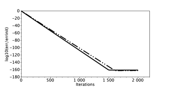
Figure 5: Numerical convergence of the complete communications method for $4\times 1$ (solid) and $2\times 2$ (dashed-dotted) subdomains

We do the same experiment for the complete communication method as we did for the auxiliary variable in §3.2. The results are shown in Figure 5. As expected, for the complete communication method, convergence is also observed up to minreal for the $2\times 2$ subdomain cases, i.e., when there are crosspoints. In practice, when using complete communication methods, the Robin parameters should be different at cross-points, see [13] for full details. In this paper, we chose not to do so and use the same $p$ at cross-points.

5 Conclusion

This paper contains two concrete propositions on how to discretize Neumann conditions at cross points in domain decomposition methods: the auxiliary variable method and complete communication. We showed three new results: first that the introduction of auxiliary variables makes it possible to prove convergence of the discretized methods for very general decompositions, including cross points, using energy estimates. Second that Neumann conditions can be split at cross points in a way minimizing artificial oscillation in the domain decomposition, and third, in the Appendix, that lumping the mass matrix in a finite element discretized optimized Schwarz method leads to better performance. We explained this by a reinterpretation at the continuous level, which shows a tangential higher order operator appearing. Its weight can even be optimized using the new concept of overlumping, and this can be done purely at the algebraic level, without need to discretize a complicated higher order operator.

We have restricted ourselves to two spatial dimensions. In higher dimensions, in addition to cross-points, there would also be cross-edges. Both the auxiliary variables method and complete communication can be adapted to higher dimensions, which is work in progress.

Appendix A (Over)lumping of the Interface mass matrix

We start with a numerical experiment, using the consistent interface mass matrix $B_{i}$ from (5) and the lumped interface mass matrix $B_{i}^{\textrm{lump}}$ from (6) in the Robin transmission condition of the OSM. We solve the Poisson equation with right hand side $f(x,y)=2(y(4.0-y)+x(4.0-x))$ on the square domain $\Omega=(0,4)^{2}$ with $3\times 3$ subdomains of equal size, and Robin parameter $p=2.0$, discretized using $Q_{1}$ finite elements with mesh size $h=1/15$. Figure 6 shows how the error decreases as a function of the iteration index in the OSM for these two choices.

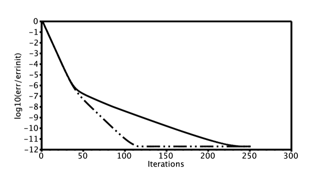
Figure 6: Convergence with lumped Robin(dashed-dotted) and consistent Robin(solid)

We see that initially the two methods converge at the same rate, but around iteration $40$, the method using the consistent mass interface matrix slows down. We show in Figure 7 snapshots of the error distribution for selected iteration indices.

Figure 7: Scaled error distribution at iteration $35$, $50$, $75$, $100$, $150$ and $200$ for OSM with consistent interface mass matrix using auxiliary variables at cross-points.

We see that a highly oscillatory mode appears in the error along the interfaces. Snapshots of the error distribution using the lumped mass matrix $B_{i}^{\textrm{lump}}$ are shown in Figure 8 for the same experiment setting.

Figure 8: Scaled error distribution at iteration $35$, $50$, $65$, $80$, $95$, $110$ for OSM with lumped interface mass matrix using auxiliary variables at cross-points.

We see that with the lumped mass matrix, the high frequency error mode along the interface is much less pronounced, and convergence is faster.

In order to understand this phenomenon, we reinterpret the effect of mass lumping at the continuous level: the difference

$$B^{\mathrm{\textrm{lump}}}_{i;j,j^{\prime}}-B_{i;j,j^{\prime}}=\begin{cases}\frac{p}{6}\sum_{j^{\prime\prime}}\lvert\bm{x}_{i;j}-\bm{x}_{i;j^{\prime\prime}}\rvert&\text{if $j^{\prime}=j$ and $\bm{x}_{i;j}$ lies on $\partial\Omega_{i}$},\\ -\frac{p}{6}\lvert\bm{x}_{i;j}-\bm{x}_{i;j^{\prime}}\rvert&\text{if $[\bm{x}_{i;j}\bm{x}_{i;j^{\prime}}]$ is an edge of $\partial\Omega_{i}$},\\ 0&\text{otherwise},\end{cases}$$

looks like the discretization of a negative, one-dimensional Laplacian. This holds technically only if the step size $h$ is constant and we are not at a cross-point. In that case, the lumped matrix actually discretizes the higher order transmission condition

$$\frac{\partial u}{\partial\bm{n}_{i}}+\frac{ph^{2}}{6}\frac{\partial^{2}u}{\partial^{2}\bm{\tau}}+pu.$$

If we could modify the value of $ph^{2}$, we would obtain a truly optimizable higher order, or Ventcell, transmission condition. This motivates the idea of overlumping: introducing a relaxation parameter $\omega$, we define

$$B^{\omega}_{i;j,j^{\prime}}:=(1-\omega)B_{i;j,j^{\prime}}+\omega B^{\mathrm{lump}}_{i;j,j^{\prime}},$$ (26)

and thus obtain a discretization of the transmission condition

$$\frac{\partial u}{\partial\bm{n}_{i}}+\omega\frac{ph^{2}}{6}\frac{\partial^{2}u}{\partial^{2}\bm{\tau}}+pu.$$ (27)

We perform now a numerical experiment with this overlumped mass matrix. For a rectangular domain $\Omega=(0,4)\times(0,2)$ with two square subdomains $\Omega_{1}=(0,2)\times(0,2)$ and $\Omega_{2}=(2,4)\times(0,2)$, we run the OSM on Laplace’s equation discretized with $Q_{1}$ finite elements and homogeneous boundary conditions, thus simulating directly the error equations. We start with a random initial guess on the interface $\{2\}\times(0,2)$. We apply $50$ Optimized Schwarz iterations. We do this for $10\times 10$, $20\times 20$, $50\times 50$ and $100\times 100$ cells per subdomains, with the Robin parameter $p$ going from $1$ to $20$ with increment of $0.5$ and the lump parameter $\omega$ going from $0$ to $100$ with increment of $0.25$. We give the optimal $p$ and $\omega$ in Table 1.

Cells in $\Omega_{i}$	Consistent	Lumped	Best
$10\times 10$	$\omega=0.0$, $p=6.0$, $\kappa=0.5791628$	$\omega=1.0$, $p=3.5$, $\kappa=0.3887587$	$\omega=10.25$, $p=1.5$, $\kappa=0.1245496$
$20\times 20$	$\omega=0.0$, $p=8.5$, $\kappa=0.6853493$	$\omega=1.0$, $p=5.0$, $\kappa=0.5222360$	$\omega=17.75$, $p=2.0$, $\kappa=0.1852617$
$50\times 50$	$\omega=0.0$, $p=14.0$, $\kappa=0.7847913$	$\omega=1.0$, $p=8.0$, $\kappa=0.6643391$	$\omega=45.0$, $p=2.5$, $\kappa=0.2863597$
$100\times 100$	$\omega=0.0$, $p=22.5$, $\kappa=0.8141025$	$\omega=1.0$, $p=12.0$, $\kappa=0.7332624$	$\omega=89.25$, $p=3.0$, $\kappa=0.3571062$

Table 1: Optimal Robin parameter $p$ and overlump factor $\omega$ with corresponding numerical convergence factor $\kappa=\exp(\log(\lVert u_{50}\rVert_{\infty}/\lVert u_{0}\rVert_{\infty})/50)$ and $2$ subdomains.

Using the asymptotic results from [10], the optimal asymptotic choice of $p$ for the consistent mass interface matrix should behave like $p=O(1/h^{1/2})$, and in the emulated Ventcell case from overlumping, we should have $p=O(1/h^{1/4})$ and $\omega=O(1/h)$, which is well what we observe.

We perform now a new numerical experiment with this overlumped mass matrix but in the presence of a single cross-point. For this experiment, we use the auxiliary variable method, see Table 2, and complete communication, see Table 3. For a square domain $\Omega=(0,4)\times(0,4)$ with four square subdomains $\Omega_{1}=(0,2)\times(0,2)$ and $\Omega_{2}=(2,4)\times(0,2)$, $\Omega_{3}=(0,2)\times(2,4)$ and $\Omega_{4}=(2,4)\times(2,4)$, we run the OSM on Laplace’s equation discretized with $Q_{1}$ finite elements and homogeneous boundary conditions, thus simulating directly the error equations. We start with a random initial guess on the interface $\{2\}\times(0,4)\cup(0,4)\times\{2\}$. We apply $50$ optimized Schwarz iterations. We do this for $10\times 10$, $20\times 20$, $50\times 50$ and $100\times 100$ cells per subdomains. We started with the Robin parameter $p$ going from $1$ to $20$ with increment of $0.5$ and the lump parameter $\omega$ going from $0$ to $100$ with increment of $0.25$. For the $100\times 100$ cells per subdomain with consistent Robin conditions case, we extended the search for the Robin parameter up to $24.5$. For the best (overlumping) case, $2\times 2$ subdomains and $10\times 10$ cells per subdomain, we extended the search for the optimal $p$ to the interval $[0.1,1]$ with increment of $0.1$.

Cells in $\Omega_{i}$	Consistent	Lumped	Best
$10\times 10$	$\omega=0.0$, $p=3.5$, $\kappa=0.7468911$	$\omega=1.0$, $p=2.0$, $\kappa=0.6833862$	$\omega=17.25$, $p=0.8$, $\kappa=0.4862979$
$20\times 20$	$\omega=0.0$, $p=5.0$, $\kappa=0.8073780$	$\omega=1.0$, $p=3.0$, $\kappa=0.7053783$	$\omega=14.75$, $p=1.5$, $\kappa=0.5045374$
$50\times 50$	$\omega=0.0$, $p=8.0$, $\kappa=0.8775996$	$\omega=1.0$, $p=4.5$, $\kappa=0.8032485$	$\omega=82.0$, $p=1.5$, $\kappa=0.5001431$
$100\times 100$	$\omega=0.0$, $p=11.0$, $\kappa=0.9102802$	$\omega=1.0$, $p=6.5$, $\kappa=0.8547884$	$\omega=122.5$, $p=2.0$, $\kappa=0.6013464$

Table 2: Optimal Robin parameter $p$ and overlump factor $\omega$ with corresponding numerical convergence factor $\kappa=\exp(\log(\lVert u_{60}\rVert_{\infty}/\lVert u_{30}\rVert_{\infty})/30)$ for $2\times 2$ subdomains using auxiliary variable method.

Cells in $\Omega_{i}$	Consistent	Lumped	Best
$10\times 10$	$\omega=0.0$, $p=3.5$, $\kappa=0.7553129$	$\omega=1.0$, $p=2.0$, $\kappa=0.6967638$	$\omega=17.75$, $p=1.0$, $\kappa=0.3989268$
$20\times 20$	$\omega=0.0$, $p=5.0$, $\kappa=0.8134911$	$\omega=1.0$, $p=3.0$, $\kappa=0.7082014$	$\omega=15.0$, $p=1.5$, $\kappa=0.4997952$
$50\times 50$	$\omega=0.0$, $p=8.0$, $\kappa=0.8778605$	$\omega=1.0$, $p=4.5$, $\kappa=0.8034476$	$\omega=86.0$, $p=1.5$, $\kappa=0.5141311$
$100\times 100$	$\omega=0.0$, $p=11.0$, $\kappa=0.9106798$	$\omega=1.0$, $p=6.5$, $\kappa=0.8528811$	$\omega=122.0$, $p=2.0$, $\kappa=0.6006753$.

Table 3: Optimal Robin parameter $p$ and overlump factor $\omega$ with corresponding numerical convergence factor $\kappa=\exp(\log(\lVert u_{60}\rVert_{\infty}/\lVert u_{30}\rVert_{\infty})/30)$ for $2\times 2$ subdomains using complete communication method. Same $p$ at cross-point as on edge.

Appendix B A simple lemma on connected graphs

Lemma B.1.

Let $\mathcal{G}$ be a connected graph. Let $V(G)$ be its set of vertices and $E(G)$ be its set of edges. Let $\phi$ be a function from $V(G)$ to $\mathbb{R}$ such that $\sum_{v\in V(G)}\phi(v)=0$. Let

$$E_{f}(G)=\{(v_{1},v_{2})\in V(G)\times V(G)\text{ s.t. }\{v_{1},v_{2}\}\in E(G)\}.$$

Then, there exists

$$\psi:E_{f}(G)\to\mathbb{R}$$

such that

$$\psi(v_{1},v_{2} )=-\psi(v_{2},v_{1})\text{ for all $(v_{1},v_{2})$ in $E_{f}(G)$},$$

$$\phi(v_{1}) =\sum_{v_{2}\text{ s.t. $(v_{1},v_{2})$ in $E_{f}(G)$}}\psi(v_{1},v_{2}).$$

Proof.

By recurrence over the number of vertices. The lemma is trivially true when the number of vertices is $1$. Suppose the lemma is true when the number of vertices is $n$ with $n\geq 1$. Let $G$ be a connected graph with $n+1$ vertices. It is well known that there exists a vertex $v$ such that $G-\{v\}$ remains connected. Since $G$ is connected, there are edges of $G$ originating from $v$. Choose $w_{0}$ adjacent to $v$. Set $\psi(v,w_{0}):=\phi(v)$, $\psi(w_{0},v):=-\phi(v)$ and $\psi(v,w):=\psi(w,v):=0$ for all other vertices $w$ adjacent to $v$. Set

$$\begin{split}\hat{\phi}:V(G)\setminus\{v\}&\to\mathbb{R}\\ w&\mapsto\begin{cases}\phi(w)&\text{if $w$ not adjacent to $v$},\\ \phi(w)-\psi(w,v)&\text{if $w$ adjacent to $v$}.\end{cases}\end{split}$$

We have $\sum_{w}\hat{\phi}(w)=\sum_{w}\phi(w)=0$. We apply the lemma on $\hat{\phi}$ and $G-\{v\}$ which is connected and get the remaining values of $\psi$. ∎

References

• [1] Abderrahmane Bendali and Yassine Boubendir. Non-overlapping domain decomposition method for a nodal finite element method. Numerische Mathematik, 103(4):515–537, 2006.
• [2] Bernard Bialecki and Maksymilian Dryja. Nonoverlapping domain decomposition with cross points for orthogonal spline collocation. Journal of Numerical Mathematics, 16(2):83–106, June 2008.
• [3] Yassine Boubendir, Abderrahmane Bendali, and M’Barek Fares. Coupling of a non-overlapping domain decomposition method for a nodal finite element method with a boundary element method. International Journal for Numerical Methods in Engineering, 73(11):1624–1650, 2008.
• [4] René Cautres, Raphaèle Herbin, and Florence Hubert. The Lions domain decomposition algorithm on non-matching cell centred finite volume meshes. IMA Journal of Numerical Analysis, 24(3):465–490, 2004.
• [5] Philippe Chevalier and Frédéric Nataf. Symmetrized method with optimized second-order conditions for the Helmholtz equation. In Domain decomposition methods, 10 (Boulder, CO, 1997), pages 400–407, Providence, RI, 1998. Amer. Math. Soc.
• [6] Bruno Després. Domain decomposition method and the helmholtz problem. In Gary C. Cohen, Laurence Halpern, and Patrick Joly, editors, Mathematical and numerical aspects of wave propagation phenomena, volume 50 of Proceedings in Applied Mathematics Series, pages 44–52. Society for Industrial and Applied Mathematics, 1991.
• [7] Victorita Dolean and Martin J Gander. Can the discretization modify the performance of Schwarz methods? In Domain Decomposition Methods in Science and Engineering XIX, pages 117–124. Springer, 2011.
• [8] Maksymilian Dryja, Wlodek Proskurowski, and Olof Widlund. A method of domain decomposition with crosspoints for elliptic finite element problems. In Blagovest Sendov, editor, Optimal Algorithms, pages 97–111, Sofia, Bulgaria, 1986. Bulgarian Academy of Sciences.
• [9] Charbel Farhat, Michel Lesoinne, Patrick Le Tallec, Kendall Pierson, and Daniel Rixen. FETI-DP: A Dual-Primal unified FETI method - part I: A faster alternative to the two-level FETI method. International Journal for Numerical Methods in Engineering, 50(7):1523–1544, 2001.
• [10] Martin J. Gander. Optimized Schwarz methods. SIAM J. Numer. Anal., 44(2):699–731, 2006.
• [11] Martin J. Gander, Laurence Halpern, and Frédéric Nataf. Optimized Schwarz methods. In Tony Chan, Takashi Kako, Hideo Kawarada, and Olivier Pironneau, editors, Twelfth International Conference on Domain Decomposition Methods, Chiba, Japan, pages 15–28, Bergen, 2001. Domain Decomposition Press.
• [12] Martin J. Gander, Florence Hubert, and Stella Krell. Optimized Schwarz algorithm in the framework of DDFV schemes. In Domain Decomposition Methods in Science and Engineering XX. Springer LNCSE, 2013. To appear.
• [13] Martin J. Gander and Felix Kwok. Best Robin parameters for optimized Schwarz methods at cross points. SIAM J. Sci. Comp., 34(4):pp. A1849–A1879, 2012.
• [14] Martin J. Gander and Felix Kwok. On the applicability of Lions’ energy estimates in the analysis of discrete optimized schwarz methods with cross points. In Domain Decomposition Methods in Science and Engineering XX, pages 475–483, 2013.
• [15] Martin J. Gander, Felix Kwok, and Kévin Santugini. Optimized Schwarz at cross points: Finite volume case. In preparation, 2013.
• [16] Martin J. Gander, Frédéric Magoulès, and Frédéric Nataf. Optimized Schwarz methods without overlap for the Helmholtz equation. SIAM J. Sci. Comput., 24(1):38–60, 2002.
• [17] David Goldberg. What every computer scientist should know about floating point arithmetic. ACM Computing Surveys, 23(1):5–48, 1991.
• [18] Laurence Halpern and Florence Hubert. A finite volume Ventcell-Schwarz algorithm for advection-diffusion equations. To appear in Sinum, 201X.
• [19] IEEE. IEEE Standard for Floating-Point Arithmetic. The Institute of Electrical and Electronics Engineers, Inc., 3 Park Avenue, New York, NY 10016-5997, USA, August 2008.
• [20] Caroline Japhet. Conditions aux limites artificielles et décomposition de domaine: Méthode oo2 (optimisé d’ordre 2). application à la résolution de problèmes en mécanique des fluides. Technical Report 373, CMAP (Ecole Polytechnique), 1997.
• [21] Caroline Japhet. Optimized Krylov-Ventcell method. Application to convection-diffusion problems. In Petter E. Bjørstad, Magne S. Espedal, and David E. Keyes, editors, Proceedings of the 9th international conference on domain decomposition methods, pages 382–389. ddm.org, 1998.
• [22] Caroline Japhet and Frédéric Nataf. The best interface conditions for domain decomposition methods: Absorbing boundary conditions. to appear in ’Artificial Boundary Conditions, with Applications to Computational Fluid Dynamics Problems’ edited by L. Tourrette, Nova Science, 2000.
• [23] Caroline Japhet, Frédéric Nataf, and Francois Rogier. The optimized order 2 method. application to convection-diffusion problems. Future Generation Computer Systems FUTURE, 18, 2001.
• [24] Axel Klawonn, Olof Widlund, and Maksymilian Dryja. Dual-primal FETI methods for three-dimensional elliptic problems with heterogeneous coefficients. SIAM J. Numer. Anal., 40(1):159–179, April 2002.
• [25] Pierre-Louis Lions. On the Schwarz alternating method. III: a variant for nonoverlapping subdomains. In Tony F. Chan, Roland Glowinski, Jacques Périaux, and Olof Widlund, editors, Third International Symposium on Domain Decomposition Methods for Partial Differential Equations , held in Houston, Texas, March 20-22, 1989, pages 202–223, Philadelphia, PA, 1990. SIAM.
• [26] Sébastien Loisel. Condition number estimates for the nonoverlapping optimized Schwarz method and the 2-Lagrange multiplier method for general domains and cross points. SIAM Journal on Numerical Analysis, 51(6):3062–3083, 2013.
• [27] Jan Mandel and Marian Brezina. Balancing domain decomposition for problems with large jumps in coefficients. Math. Comp., 65:1387–1401, 1996.
• [28] Alfio Quarteroni and Alberto Valli. Domain Decomposition Methods for Partial Differential Equations. Oxford Science Publications, 1999.
• [29] Barry F. Smith, Petter E. Bjørstad, and William Gropp. Domain Decomposition: Parallel Multilevel Methods for Elliptic Partial Differential Equations. Cambridge University Press, 1996.
• [30] Pat H. Sterbenz. Floating-point computation. Prentice-Hall series in automatic computation. Prentice-Hall, 1973.
• [31] Andrea Toselli and Olof Widlund. Domain Decomposition Methods - Algorithms and Theory, volume 34 of Springer Series in Computational Mathematics. Springer, 2004.