Maxwell-Chern-Simons vortices in a CPT-odd Lorentz-violating Higgs Electrodynamics

Abstract

We have studied BPS vortices in a CPT-odd and Lorentz-violating Maxwell-Chern-Simons-Higgs (MCSH) electrodynamics attained from the dimensional reduction of the Carroll-Field-Jackiw-Higgs model. The Lorentz-violating parameter induces a pronounced behavior at origin (for the magnetic/electric fields and energy density) which is absent in the MCSH vortices. For some combination of the Lorentz-violating coefficients there always exist a sufficiently large winding number $n_{0}$ such that for all $|n|\geq|n_{0}|$ the magnetic field flips its signal, yielding two well defined regions with opposite magnetic flux. However, the total magnetic flux remains quantized and proportional to the winding number.

I Introduction

Vortex configurations constitute an important branch of research, common to condensed matter and high energy physics. This interconnection was established since the seminal works by Abrikosov ANO1 and Nielsen-Olesen ANO2 , which demonstrated the existence of electrically neutral vortices in type-II superconducting systems and in field theory models, respectively. Since then, vortex solutions have become a theoretical field of increasing interest, reinforced with the works arguing the existence of BPS (Bogomol’nyi, Prasad, Sommerfeld) solutions BPS . BPS vortices were found in the Chern-Simons-Higgs model CSV and in the Maxwell-Chern-Simons-Higgs (MCSH) model MCS , with additional investigations involving nonminimal coupling CSV1 and other aspects CSV2 ; Bolog . Recently it has been shown the existence of generalized Maxwell-Higgs and Chern-Simons vortices Hora1 in the context of k-field theories kfield ; GC which have been a fertile environment for studying new topological defects solutions kfield2 . The existence of charged BPS vortices in a generalized Maxwell-Chern-Simons-Higgs model was also demonstrated in Ref. Cadu-last , while the duality between vortices and planar Skyrmions in BPS theories has also been addressed Adam . Unusual vortex configurations in condensed matter systems, endowed with magnetic flux reversion Brevers and fractional quantization Frac , have also caught attention in the latest years.

Lorentz violating theories have been focus of strong interest since the proposal of the standard model extension (SME) Colladay ; Samuel , whose gauge sector was intensively scrutinized in many respects KM ; Klink ; NM . The study of topological defects in Lorentz-violating scenarios was initially conducted for scalar systems defects Defects . The existence of monopole solutions in the presence of Lorentz violation was regarded in the context of the Carroll-Field-Jackiw electrodynamics Monopole1 . Topological defects were also examined in a broader framework of field theories endowed with tensor fields that spontaneously break the Lorentz symmetry Seifert .

The pioneering investigation about BPS vortex solutions in the presence of CPT-even Lorentz-violating terms of the SME was performed in Refs. Carlisson1 ; Carlisson2 , following the idea of finding new defect solutions in modified theoretical frameworks. In Ref. Carlisson1 , uncharged BPS vortices were found in an Abelian Maxwell-Higgs model supplemented with CPT-even Lorentz-violating terms belonging to the Higgs and gauge sectors of the SME. The Lorentz-violating BPS vortices are compactlike and could present fractional quantization of the magnetic flux. In a similar context, it was shown that the parity-odd sector of the CPT-even term $\left(K_{F}\right)^{\mu\alpha\nu\beta}$ allows the existence of electrically charged BPS vortices in absence of the Chern-Simons term Carlisson2 , endowed with magnetic flux reversion. The study of vortex configurations in Lorentz-violating models has been an issue of active investigation recently Belich .

Sor far, no vortex investigation was performed in a CPT-odd and Lorentz-violating environment. The aim of this paper is to study BPS vortices in the Lorentz-violating planar Maxwell-Carroll-Field-Jackiw electrodynamics, trying to answer what are the BPS vortex solutions supported by this planar version of CPT-odd gauge sector of the SME. We highlight the features of the corresponding BPS solutions, which possess magnetic flux reversion: a remarkable feature induced by Lorentz-violation which may find applications in some vortex systems of condensed matter physics Brevers ; Frac . We thus start from a planar Lorentz-violating Maxwell-Chern-Simons model attained via the dimensional reduction of the CPT-odd Maxwell-Carroll-Field-Jackiw electrodynamics coupled to the Higgs sector, examined in Ref. EPJC1 . In Sec. II, we present the model and implement the BPS formalism to attain the self-dual first order equations describing the topological vortices. In Sec. III, we use the vortex ansatz to show that our solutions satisfy the usual boundary conditions and behave as Abrikosov-Nielsen-Olesen vortices. Also, the results of the numerical analysis are presented, revealing charged vortex profiles that recover the MCSH solutions in the asymptotic region, and may strongly differ from these ones near the origin. Finally, in Sec. IV, we give our remarks and conclusions.

II The theoretical model and BPS formalism

The Maxwell-Carroll-Field-Jackiw-Higgs model EPJC1 in $(1+3)-$dimensions is given by

$$\mathcal{L} = -\frac{1}{4}F_{\hat{\mu}\hat{\nu}}F^{\hat{\mu}\hat{\nu}}-\frac{1}{4}\epsilon^{\hat{\mu}\hat{\nu}\hat{\rho}\hat{\sigma}}\left(k_{AF}\right)_{\hat{\mu}}A_{\hat{\nu}}F_{\hat{\rho}\hat{\sigma}}$$

$$+\left|D_{\hat{\mu}}\phi\right|^{2}-V\left(\left|\phi\right|\right),$$

where $\hat{\mu},\hat{\nu},\hat{\rho},\hat{\sigma}=0,1,2,3$ and $D_{\hat{\mu}}\phi=\partial_{\hat{\mu}}\phi-ieA_{\hat{\mu}}\phi$, the covariant derivative. The dimensional reduction of this Lagrangian provides a kind of MCSH model modified by Lorentz-violating (LV) terms which play the role of coupling constants between the neutral scalar field $\left(\psi\right)$ and the abelian gauge field $(A_{\mu})$. Thus, the Lorentz-violating MCSH model is described by the following Lagrangian density

$$\mathcal{L} = -\frac{1}{4}F_{\mu\nu}F^{\mu\nu}+\frac{1}{4}s\,\epsilon^{\nu\rho\sigma}A_{\nu}F_{\rho\sigma}+\left|D_{\mu}\phi\right|^{2}$$

$$+\frac{1}{2}\partial_{\mu}\psi\partial^{\mu}\psi-e^{2}\psi^{2}\left|\phi\right|^{2}-U\left(\left|\phi\right|,\psi\right)$$

$$-\frac{1}{2}\epsilon^{\mu\rho\sigma}\left(k_{AF}\right)_{\mu}A_{\rho}\partial_{\sigma}\psi-\frac{1}{2}\epsilon^{\mu\rho\sigma}\left(k_{AF}\right)_{\mu}\psi~{}\partial_{\rho}A_{\sigma},$$

where $\psi$ is the scalar neutral field stemming from the dimensional reduction ($\psi=A_{\hat{3}}$), the Lorentz-violating parameter $s=\left(k_{AF}\right)_{\hat{3}}$ plays the role of a Chern-Simons coupling, $\left(k_{AF}\right)_{\mu}$ is the (1+2)-dimensional CFJ vector background which couples the neutral and gauge fields. Here, $D_{\mu}\phi=\partial_{\mu}\phi-ieA_{\mu}\phi$ defines the covariant derivative, while the potential, $U\left(\left|\phi\right|,\psi\right)$, conveniently defined to provide BPS solutions, is

$$U\left(\left|\phi\right|,\psi\right)=\frac{1}{2}\left[ev^{2}-e\left|\phi\right|^{2}-s\psi\right]^{2}.$$ (3)

The stationary Gauss’s law and Ampere’s law are

$$\partial_{j}\partial_{j}A_{0}-sB-\epsilon_{ij}\left(k_{AF}\right)_{i}\partial_{j}\psi=2e^{2}A_{0}\left|\phi\right|^{2},$$ (4)

$$\epsilon_{kj}\partial_{j}B-s\epsilon_{kj}\partial_{j}A_{0}+\left(k_{AF}\right)_{0}\epsilon_{kj}\partial_{j}\psi=eJ_{k},$$ (5)

where $J_{k}$ is the spatial component of the current density, $J^{\mu}=i\left[\phi\left(D^{\mu}\phi\right)^{\ast}-\phi^{\ast}D^{\mu}\phi\right]$.

The stationary equations of motion of the Higgs and neutral fields read

$$0 = \partial_{k}\partial_{k}\phi-2ieA_{k}\partial_{k}\phi+e^{2}\left(A_{0}\right)^{2}\phi$$

$$-e^{2}\left(A_{k}\right)^{2}\phi-e^{2}\psi^{2}\phi-\frac{\partial U}{\partial\phi^{\ast}},$$

$$0 = \partial_{j}\partial_{j}\psi-\left(k_{AF}\right)_{0}B-\epsilon_{ij}\left(k_{AF}\right)_{i}\partial_{j}A_{0}$$

$$-2e^{2}\psi\left|\phi\right|^{2}-\frac{\partial U}{\partial\psi},$$

respectively.

The stationary energy density $\left(\mathcal{E}\right)$ associated with Lagrangian (II), is

$$\mathcal{E} = \frac{1}{2}B^{2}+\frac{1}{2}\left[ev^{2}-e\left|\phi\right|^{2}-s\psi\right]^{2}+\left|D_{j}\phi\right|^{2}$$

$$+\frac{1}{2}\left(\partial_{j}A_{0}\right)^{2}+\frac{1}{2}\left(\partial_{j}\psi\right)^{2}+e^{2}A_{0}^{2}\left|\phi\right|^{2}+e^{2}\psi^{2}\left|\phi\right|^{2},$$

where the condition $\left(k_{AF}\right)_{0}=0$ was imposed in order to assuring the positiveness of the energy density. Thus, in the present approach, only spatial components of the (1+2)-dimensional Carroll-Field-Jackiw vector background contribute.

In the following we focus our attention on the development of a BPS framework BPS which provides first order differential equations consistent with the second order equations (4)–(LABEL:Neutral_1). With this aim, we first impose the following condition on the neutral field $\psi$:

$$\psi=\mp A_{0},$$ (9)

which is similar to that appearing in the context of the  MCSH vortex configurations MCS ; CSV2 ; Bolog . By substituting (9) in Eq. (LABEL:energy_0), we achieve

$$\mathcal{E} = \frac{1}{2}B^{2}+\frac{1}{2}\left[ev^{2}-e\left|\phi\right|^{2}\pm sA_{0}\right]^{2}$$

$$+\left|D_{j}\phi\right|^{2}+\left(\partial_{j}A_{0}\right)^{2}+2e^{2}A_{0}^{2}\left|\phi\right|^{2}.$$

After converting the two first terms in quadratic form, and by using the identity

$$\left|D_{j}\phi\right|^{2}=\left|D_{\pm}\phi\right|^{2}\pm e\left|\phi\right|^{2}B\pm\frac{1}{2}\epsilon_{ab}\partial_{a}J_{b},$$ (11)

with $D_{\pm}\phi=D_{1}\phi\pm iD_{2}\phi$, the energy density becomes

$$\mathcal{E} = \frac{1}{2}\left[B\mp\left(ev^{2}-e\left|\phi\right|^{2}\pm sA_{0}\right)\right]^{2}$$

$$+\left|D_{\pm}\phi\right|^{2}\pm ev^{2}B\pm\frac{1}{2}\epsilon_{ab}\partial_{a}J_{b}$$

$$+\left(\partial_{j}A_{0}\right)^{2}+sBA_{0}+2e^{2}A_{0}^{2}\left|\phi\right|^{2}.$$

By substituting Eq. (9) in the Gauss law (4), it is possible to transform the last three terms in a total derivative, such that the energy density can be written as

$$\mathcal{E} = \frac{1}{2}\left[B\mp\left(ev^{2}-e\left|\phi\right|^{2}\pm sA_{0}\right)\right]^{2}$$

$$+\left|D_{\pm}\phi\right|^{2}\pm ev^{2}B+\partial_{a}\mathcal{J}_{a},$$

with $\mathcal{J}_{a}$ defined as

$$\mathcal{J}_{a}=\pm\frac{1}{2}\epsilon_{ab}J_{b}+A_{0}\partial_{a}A_{0}\mp\frac{1}{2}\epsilon_{ab}\left(k_{AF}\right)_{b}A_{0}^{2}.$$ (14)

The energy density (LABEL:E_den) is minimized by imposing that the quadratic terms must be null, which leads to the BPS conditions of this model,

$$D_{\pm}\phi=0~{},$$ (15)

$$B=\pm\left(ev^{2}-e\left|\phi\right|^{2}\right)+sA_{0}.$$ (16)

which are the same ones of the MCSH model MCS .

These BPS equations, and the Gauss law, now written as

$${\partial_{j}\partial_{j}A_{0}-sB\pm\epsilon_{ij}\left(k_{AF}\right)_{i}\partial_{j}A}_{0}{=2e^{2}A_{0}\left|\phi\right|^{2},}$$ (17)

describe topological vortices in this Lorentz-violating MCSH framework.

Under BPS conditions, the energy density becomes

$$\mathcal{E}_{BPS}=\pm ev^{2}B+\partial_{a}\mathcal{J}_{a}.$$ (18)

After integrating under appropriated boundary conditions (see Eqs. (21) and (22)), one achieves the BPS energy

$$E_{BPS}={\pm}ev^{2}\int d^{2}rB={\pm}2\pi v^{2}n,$$ (19)

which is proportional to the quantized magnetic flux, $\Phi_{B}=2\pi n/e,\$where $n$ is the winding number of the vortex configuration.

III Charged vortex configurations

Specifically, we look for radially symmetric solutions using the standard static vortex Ansatz

$$\phi=vg\left(r\right)e^{in\theta},~{}A_{\theta}=-\frac{a\left(r\right)-n}{er},~{}A_{0}=A_{0}(r),$$ (20)

where $n$ represents the winding number of the topological vortex, the scalar functions $a\left(r\right),$ $g\left(r\right)$ and $\omega\left(r\right)$ are regular in $r=0$ and at $r\rightarrow\infty$. As usual, the fields $g\$and $a$ satisfy the following boundary conditions

$$g\left(0\right)=0,\;a\left(0\right)=n,\\$$ (21)

$$g\left(\infty\right)=1,\,a\left(\infty\right)=0.$$ (22)

The boundary conditions satisfied by the field $A_{0}$ will be explicitly established in subsection III.1.

The Ansatz (20) allows to express the magnetic field in a simple way

$$B=-\frac{a^{\prime}}{er}.$$ (23)

The BPS equations (15,16) are rewritten as

$$g^{\prime} = \pm\frac{ag}{r}\,,$$ (24)

$$B=-\frac{a^{\prime}}{er}=\pm ev^{2}\left(1-g^{2}\right)+sA_{0}\,,$$ (25)

whereas the Gauss law (17) reads as

$$A_{0}^{\prime\prime}+\frac{A_{0}^{\prime}}{r}-sB\mp\left(k_{AF}\right)_{\theta}\left(A_{0}^{\prime}+\frac{A_{0}}{2r}\right)-2e^{2}v^{2}g^{2}A_{0}=0,$$ (26)

where the upper(lower) signal corresponds to $n>0$($n<0$).  Note that $\left(k_{AF}\right)_{\theta}$ is the only component of the $(1+2)-$dimensional Carroll-Field-Jackiw background compatible with radially symmetric solutions, that is, $\left(k_{AF}\right)_{\theta}$ is the only CFJ component remaining in the equations above describing the BPS solutions after the Ansatz (20) is implemented.  Note that it does not mean the radial component $\left(k_{AF}\right)_{r}$ was taken as null; it simply does not participate in the formation of radially symmetric vortices. This fact was also observed in the parity-odd coefficients $\kappa_{0i}$ of the symmetric tensor $\kappa_{\mu\nu}$ of the LV and CPT-even model analyzed in Ref. Carlisson2 , where only the component $\kappa_{0\theta}$ has contributed after the ansatz implementation.

From the set of equations (24)-(26), we can observe that, for fixed $s$ and considering the solutions for $n>0$, the correspondent solutions for $n<0$ can be attained by doing $g\rightarrow g~{},\ a\rightarrow-a,~{}A_{0}\rightarrow-A_{0}$ and $\left(k_{AF}\right)_{\theta}\rightarrow-\left(k_{AF}\right)_{\theta}$. We can also note that, for $n$ and $\left(k_{AF}\right)_{\theta}$ fixed, under the change $s\rightarrow-s$, the new solutions can be obtained by doing $g\rightarrow g~{},\ a\rightarrow a~{},~{}A_{0}\rightarrow-A_{0}$. And, by setting $\left(k_{AF}\right)_{\theta}=0$, we recover the solutions of the MCSH model with $s$ playing the role of the Chern-Simons parameter.

Using the BPS equations (24)-(25) and the Gauss law (26), we rewrite the BPS energy density (18) as a sum of quadratic terms

$$\mathcal{E}_{BPS}=B^{2}+2v^{2}\left(g^{\prime}\right)^{2}+{2}e^{2}v^{2}\left({g}A_{0}\right)^{2}+\left(A_{0}^{\prime}\right)^{2},$$ (27)

showing that it is a positive-definite quantity for all values of $s$ and ${\left(k_{AF}\right)_{\theta}}$.

III.1 Analysis of the boundary conditions

We begin discussing the behavior of the solutions of Eqs. (24-26) when $r\rightarrow 0$. Using the power series method, one achieves

$$g\left(r\right) = G_{n}r^{n}-\frac{G_{n}\left(e^{2}v^{2}+e{{\omega_{{0}}}}s\right)}{4}r^{n+2}$$

$$\mp\frac{G_{n}e\omega_{0}s{\left(k_{AF}\right)_{\theta}}}{18}r^{n+3}+{\mathcal{\ldots}}$$

$$a\left(r\right) = n-\frac{\left(e^{2}v^{2}+e{{\omega_{{0}}}}s\right)}{2}r^{2}\mp\frac{e\omega_{0}s{\left(k_{AF}\right)_{\theta}}}{6}r^{3}+{\mathcal{\ldots}}$$

$$A_{0}\left(r\right) = \omega_{0}\pm\frac{{\omega_{{0}}\left(k_{AF}\right)_{\theta}}}{2}r$$

$$+\frac{4s\left(ev^{2}+{{\omega_{{0}}}}s\right)+3\left[{\left(k_{AF}\right)_{\theta}}\right]^{2}\omega_{0}}{16}r^{2}+{\mathcal{\ldots}}$$

where $\omega_{0}=A_{0}\left(0\right)$, and, as it happens in the usual MCSH vortex configurations, $\omega_{{0}}$ depends on the boundary conditions above and it is numerically determined. The first two equations confirm the boundary conditions imposed in (21), while the last one allows to impose the following condition on the field $A_{0}$ at origin

$$A_{0}^{\prime}\left(0\right)=\pm\frac{{\omega_{{0}}\left(k_{AF}\right)_{\theta}}}{2},$$ (31)

The asymptotic behavior when $r\rightarrow+\infty$ for the fields $g\left(r\right),~{}a\left(r\right)$ and $A_{0}\left(r\right)$ is

$$1-g\left(r\right) \sim r^{-1/2}e^{-\beta r},$$

$$a\left(r\right) \sim r^{1/2}e^{-\beta r},$$ (32)

$$A_{0}\left(r\right) \sim r^{-1/2}e^{-\beta r},$$

where $\beta$ is a positive real number given by

$$\beta_{\pm} = \frac{1}{2}\sqrt{\left(\kappa_{\pm}\right)^{2}+8e^{2}v^{2}\ }-\frac{\kappa_{\pm}}{2},~{}\ \$$ (33)

$$\kappa_{\pm} = \sqrt{s^{2}+\frac{\left[{\left(k_{AF}\right)_{\theta}}\right]^{2}}{4}}\pm\frac{{\left(k_{AF}\right)_{\theta}}}{2}.$$ (34)

where the signal $+\left(-\right)$ stands for $n>0$ $\left(n<0\right)$. It confirms the boundary conditions (22) for the fields $g$, $a,$ but it also provides the boundary condition at $r\rightarrow\infty$ for the field $A_{0}$:

$$A_{0}\left(\infty\right)=0.$$ (35)

We observe that for fixed $s$ and ${n>0}$, the $\beta_{+}\$parameter takes higher values if ${\left(k_{AF}\right)_{\theta}}<0.$ We can consider two limiting values,

$$\lim_{{\left(k_{AF}\right)_{\theta}\rightarrow-\infty}}\beta_{+}=ev\sqrt{2},~{}\ \ \lim_{{\left(k_{AF}\right)_{\theta}\rightarrow+\infty}}\beta_{+}=0,$$ (36)

between which the parameter $\beta_{+}$ varies continually. It allows to affirm the profiles with $\left(k_{AF}\right)_{\theta}<0$ converge more quickly for their saturation values than those with $\left(k_{AF}\right)_{\theta}>0$. For $\left(k_{AF}\right)_{\theta}=0$ and fixed $s$, the behavior of $\beta$ is similar to the one of the BPS vortices coming from the MCSH model.

III.2 Numerical solutions

We now introduce the dimensionless variable $\rho=evr$ and implement the following changes in the fields,

$$g\left(r\right)\rightarrow\bar{g}\left(\rho\right),\ a\left(r\right)\rightarrow\bar{a}\left({\rho}\right),~{}A_{0}\left(r\right)\rightarrow v\bar{\omega}\left(\rho\right),$$

$$B(r)\rightarrow ev^{2}\bar{B}\left(\rho\right),~{}~{}\mathcal{E}(r)\rightarrow v^{2}\bar{\mathcal{E}}\left(\rho\right).$$

and rescaling the LV coefficients

$$\left(k_{AF}\right)_{\theta}\rightarrow ev\lambda,~{}s\rightarrow ev\bar{s},$$ (37)

where now $\lambda$ represents the (1+2)-dimensional CFJ parameter. Thereby, the expressions (24)-(26) are written in a dimensionless form as

$$\bar{g}^{\prime}=\pm\frac{\bar{a}\bar{g}}{\rho}\,,$$ (38)

$$\bar{B}=-\frac{\bar{a}^{\prime}}{\rho}=\pm\left(1-g^{2}\right)+\bar{s}\bar{\omega}\,,$$ (39)

$$\bar{\omega}^{\prime\prime}+\frac{\bar{\omega}^{\prime}}{\rho}-\bar{s}\bar{B}\mp\lambda\left(\bar{\omega}^{\prime}+\frac{1}{2}\frac{\bar{\omega}}{\rho}\right)-2\bar{g}^{2}\bar{\omega}=0\,,$$ (40)

while the dimensionless version of the BPS energy density is

$$\bar{\mathcal{E}}_{BPS}=\bar{B}^{2}+2\frac{\bar{a}^{2}\bar{g}^{2}}{\rho^{2}}+{2\bar{g}^{2}\bar{\omega}}^{2}+\left(\bar{\omega}^{\prime}\right)^{2}.$$ (41)

We have performed the numerical analysis by considering three different values for the LV parameter, $\lambda=-1,0,+1,$ and for the winding numbers, $n=1,6,15$, while the Chern-Simons-like parameter is kept fixed, $\bar{s}=1.$ The value $\lambda=0$ reproduces the profiles of the MCSH vortices MCS ; CSV2 which are depicted by green lines. Blue lines denote the BPS solution with $\lambda=-1$ and red lines the ones for $\lambda=+1$. The winding number is specified in the following way: dotted lines $\left(n=1\right)$, dashed lines $\left(n=6\right),$ and solid lines $\left(n=15\right)$. The resultant profiles for the topological solutions are depicted in Figs. 1–6. All legends are summarized in Fig. 1.

Fig. 1 depicts the profiles of the Higgs field. For $n=1$ the profiles are very similar to the MCSH ones ($\lambda=0$ case), but begin to differ from them for increasing values of the winding number. In general, the profiles with negative values of the CFJ parameter saturate more quickly than those with positive values, in accordance with Eq. (33).

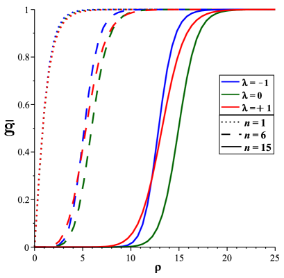
Figure 1: Scalar field $\bar{g}(\rho)$ (Blue lines for $\lambda=-1$, red lines for $\lambda=+1$. Green lines for $\lambda=0$, represents the BPS solutions for the MCSH model).

Fig. 2 shows the profiles of the vector field. For $n=1$ the profiles are very similar to the MCSH ones ($\lambda=0$ case) but for $n>1,$ near to the origin, the vector field magnitude can increase (for $\lambda=-1)$ or decrease (for $\lambda=1)$ in relation to the MCSH profiles. Near to the origin, the first (second) behavior is associated a negative (positive) magnetic field, as it is observed in Fig. 3. For $\rho\gg 0,$ the profiles always go to zero approaching the MCSH ones. Furthermore, for $\lambda=-1$ the vector field presents a region with increasing magnitude, which is compatible with a sharpened negative magnetic field around the origin. On the other hand, for $\lambda=+1$, the vector field decreases for increasing radius, providing a positive magnetic field which also engenders a sharpened structure around the origin.

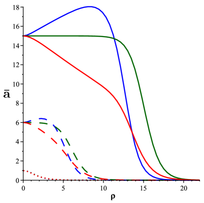
Figure 2: Vector potential $\bar{a}(\rho)$ (Blue lines for $\lambda=-1$, red lines for $\lambda=+1$, green lines for $\lambda=0$).

The magnetic field behavior is represented in Fig. 3. For $n=1$ (and different $\lambda$ values) are very similar to the MCSH one, except near the origin, where the amplitude increases with $\lambda$ (see insertion with dotted lines in Fig. 3). Already, for $n>1,$ the magnetic profiles display two localized structures that define two well-defined domains: the first one is a pronounced magnitude flux region centered at the origin, which can be positive or negative depending on the sign of $\lambda$; the second one is a lump-like region whose maximum is located in an intermediary radial distance, being compatible with a ring-like magnetic field configuration (typical of the MCSH model) whose radius increases with $n.$ The behavior near the origin changes strongly in accordance with the sign of $\lambda$: for $\lambda=1$, $B(0)>0,$ while for $\lambda=-1,$ it holds $B(0)\,<0.$ Hence, for $\lambda=-1$ there occurs magnetic field flux inversion, once the initially negative magnetic field becomes positive for $\rho>\rho_{\ast}$, with $B(\rho_{\ast})=0$ (see the blue curves for $n=6$ and $n=15$ in Fig. 3). For $\lambda=-1$  and $n\gg 1,$ the magnetic field saturates at the origin as $B(0)=-1.017$. Further, for $n>1$ and $\lambda=1$ the profiles are always positive, varying from the strong flux region centered at the origin to the ring-like region existing for an intermediary radial coordinate. For $\lambda=1$ and $n\gg 1$ the magnetic field saturates as $B(0)=0.553$. Despite this complex scenario, the total magnetic flux is positive and proportional to $n$, regardless the $\lambda$ value.

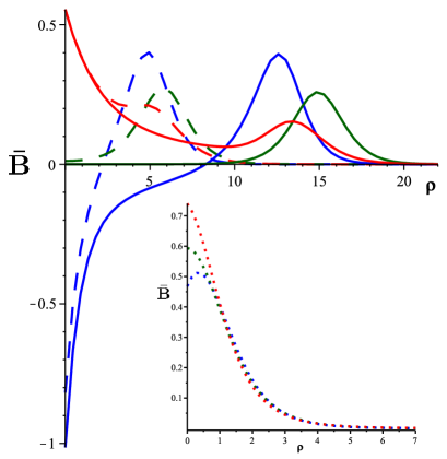
Figure 3: Magnetic field $\bar{B}(\rho)$ (Blue lines for $\lambda=-1$, red lines for $\lambda=+1$, green lines for $\lambda=0$).

The scalar potential profiles, as appearing in Fig. 4, are negative throughout the radial axis, for all values of $n$ and $\lambda$. Near to the origin, for all $n\geq 1$, the LV profiles are different from the usual MCSH solutions, with amplitudes increasing with negative $\lambda$.

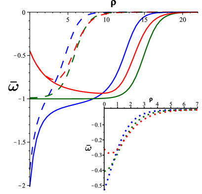
Figure 4: Scalar potential $\bar{\omega}(\rho)$ (Blue lines for $\lambda=-1$, red lines for $\lambda=+1$, green lines for $\lambda=0$. Small figure with dotted lines are the solutions for $n=1$).

On the other hand, far from the origin, the LV profiles closely follow the behavior of the MCSH solutions (green lines). Near the origin, for $\lambda=-1,$ the LV profiles present an inverted pronounced form whose amplitude saturates at $\bar{\omega}(0)=-2.017$ (for $n\gg 1);$ for $\lambda=1,$ the profiles display a conical-shaped profile whose amplitude saturates as $\bar{\omega}(0)=-0.446$. Note that both solutions deviate sensibly from the MCSH $\left(\lambda=0\right)$ value at origin, $\bar{\omega}(0)=-1.0$. It is clear that the profile with $\lambda=-1$ decays faster than the one with $\lambda=1,$ as expected.

Fig. 5 contains the electric field profiles. Even for $n=1,$ these profiles are quite different at the origin neighborhood, where it holds: $\bar{\omega}^{\prime}(0)>0$ for $\lambda=-1$, $\bar{\omega}^{\prime}(0)=0$ for $\lambda=0,$ and $\bar{\omega}^{\prime}(0)<0$ for $\lambda=1$, changing a little for intermediary radius, and becoming very similar to the MCSH ones only far from the origin (see insertion with dotted curves in Fig. 5).

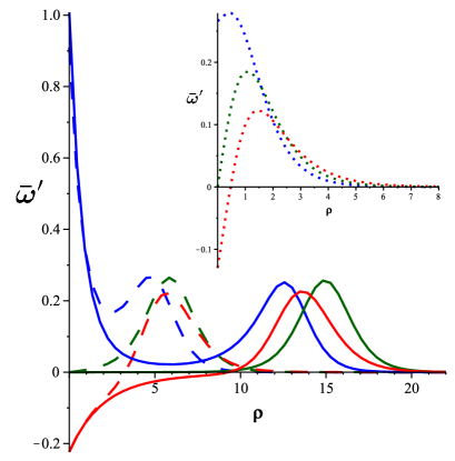
Figure 5: Electric field $\bar{\omega}^{\prime}(\rho)$. (Blue lines for $\lambda=-1$, red lines for $\lambda=+1$, green lines for $\lambda=0$).

For $n>1,$ the electric field profiles display two localized significant structures, similarly to the magnetic field behavior. In the case $\lambda=-1$, the profiles are always positive, and there is a narrow cone centered at origin, whose amplitude saturates as $\bar{\omega}^{\prime}(0)=$ $1.008$ $\left(\text{for }n\gg 1\right)$, and a positive lump-like region localized in an intermediary radial coordinate. On the other hand, for $\lambda=+1$, the electric field becomes negative near to the origin, yielding an inverted cone with smaller amplitude, which saturates as $\bar{\omega}^{\prime}(0)=$ $-0.223$ for $n\gg 1$. Further, as one goes away from the origin, the electric field changes its sign, becomes positive forming a ring-like structure around the origin, and vanishes for $\rho\rightarrow\infty$. Note that the LV electric solutions, similarly to the magnetic ones, differ from the usual MCSH ones mainly due the behavior near the origin: while the MCSH solutions are null at this point, the LV parameter may induce positive or negative electric fields in the origin neighborhood. This pattern is shared by the BPS energy density profiles.

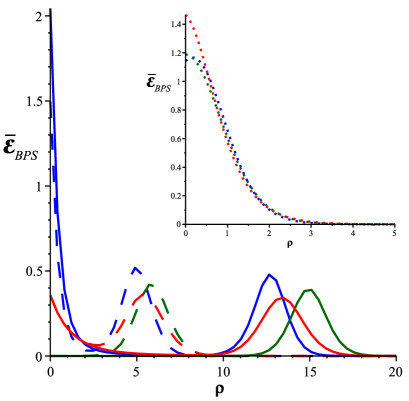
Figure 6: BPS energy density $\bar{\mathcal{E}}_{{}_{BPS}}(\rho)$. (Blue lines for $\lambda=-1$, red lines for $\lambda=+1$. Green lines for $\lambda=0$).

The BPS energy density profiles are shown in Fig. 6. For $n=1$, the profiles are lumps centered at the origin with differing amplitudes, which overlap with each other far from $\rho=0$ (see insertion with dotted curves in Fig. 6). When $n\gg 1$ and $\lambda=\pm 1$, the BPS energy density profiles present two well-pronounced regions, in accordance with the profiles of the magnetic and electric fields. The first one is a peak centered at the origin whose amplitude saturates at $0.356$ $\left(\text{for }\lambda=+1\right)$ and at $2.052$ $\left(\text{for }\lambda=-1\right)$. This concentration of energy at the origin is not present in the MCSH model. The second one is a lump-shaped region located at an intermediary distance from the origin, whose radius increases with $n,$ as it happens in the MCSH model. For each value of $n,$ the ring radius follow the inequality: $\rho_{\lambda=-1}\lesssim\rho_{\lambda=1}\lesssim\rho_{\lambda=0}$.

IV Conclusions and remarks

In this work, we have considered a Lorentz-violating planar electrodynamics, attained from the dimensional reduction of the Maxwell-Carroll-Field-Jackiw-Higgs model, as a theoretical environment for studying charged BPS vortex configurations. After writing the stationary equations of motion and the energy density, the radially symmetric usual vortex Ansatz was implemented, keeping only one Lorentz-violating parameter in the equations of the system. By manipulating the energy density, the BPS equations were obtained, confirming the existence of BPS solutions for such a model. The BPS energy remains connected with the magnetic flux quantization, as it is usual.

The numerical simulations were performed for different values of the Lorentz-violating parameter, and distinct winding numbers. For $n=1$, at the origin, the solutions sometimes present notable deviations from the MCSH profiles. However for large radius they closely follow the behavior of the MCSH ones. In general, the deviation is more accentuated for increasing winding number values.  For $n>1$, the LV profiles keep some similarity to the usual MCSH solutions in the large radius region but decay in accordance with its respective mass scale: $\beta_{\lambda<0}>\beta_{\lambda=0}>\beta_{\lambda>0}$.  The role played by the LV parameter becomes more pronounced at the origin, where it generates a peaked profile (absent in the MCSH solutions) in the magnetic/electric field and the energy density profiles. When $\lambda<0$ the magnetic field assumes negative values near the origin. However, for a sufficiently large radius, it flips its signal, providing two regions with opposite magnetic flux. The flipping of the magnetic flux represents a remarkable feature induced by Lorentz-violation, which may find applications in condensed matter systems endowed with magnetic flux reversion Brevers ; Frac . This feature was also observed in charged vortex configurations defined in the context of the CPT-even and nonbirefringent Lorentz-violating model of Ref. Carlisson2 .

The analysis performed above can be extended for all values of $\bar{s}$ and $\lambda$. For $n>0$, a fixed $\bar{s}$, and $\lambda>0,$ there are always two well defined regions with positive magnetic flux, occurring no magnetic field reversion. On the other hand, for fixed $\bar{s}$ and $\lambda<0,$ there always exists a sufficiently large winding number $n_{0}$ such that for $n>n_{0}$ the magnetic field reverses its signal. Consequently, there are always two well defined regions with opposite magnetic flux. A similar result is obtained for $n<0$. However, in all cases the total magnetic flux remains quantized and proportional to the winding number.

Acknowledgements

The authors thank to CAPES, CNPq and FAPEMA (Brazilian agencies) for financial support.

References

- (1) A. Abrikosov, Sov. Phys. JETP 32, 1442 (1957).
- (2) H. Nielsen, P. Olesen, Nucl. Phys. B 61, 45 (1973).
- (3) E. B. Bogomol’nyi, Sov. J. Nuc. Phys. 24, 449 (1976); M. Prasad and C. Sommerfield, Phys. Rev. Lett. 35, 760 (1975).
- (4) R. Jackiw and E. J. Weinberg, Phys. Rev. Lett. 64, 2234 (1990); R. Jackiw, K. Lee, and E.J. Weinberg, Phys. Rev. D42, 3488 (1990); J. Hong, Y. Kim, and P.Y. Pac, Phys. Rev. Lett. 64, 2230 (1990); G.V. Dunne, Self-Dual Chern-Simons Theories (Springer, Heidelberg, 1995).
- (5) C.k. Lee, K.M. Lee, H. Min, Phys. Lett. B 252, 79 (1990).
- (6) P.K. Ghosh, Phys. Rev. D 49, 5458 (1994); T. Lee and H. Min, Phys. Rev. D 50, 7738 (1994).
- (7) N. Sakai and D. Tong, J. High Energy Phys. 03 (2005) 019; G. S. Lozano, D. Marques, E. F. Moreno, and F. A. Schaposnik, Phys. Lett. B 654, 27 (2007).
- (8) S. Bolognesi and S.B. Gudnason, Nucl. Phys. B 805, 104 (2008).
- (9) D. Bazeia, E. da Hora, C. dos Santos, and R. Menezes, Phys. Rev. D 81, 125014 (2010); D. Bazeia, E. da Hora, R. Menezes, H. P. de Oliveira, and C. dos Santos, Phys. Rev. D 81, 125016 (2010); D. Bazeia, E. da Hora, C. dos Santos, R. Menezes, Eur. Phys. J. C 71, 1833 (2011).
- (10) E. Babichev, Phys. Rev. D 74, 085004 (2006); Phys. Rev. D 77, 065021 (2008).
- (11) N. Arkani-Hamed, H.-C. Cheng, M. A. Luty, and S. Mukohyama, J.High Energy Phys. 05, 074 (2004); N. Arkani-Hamed, P. Creminelli, S. Mukohyama, and M. Zaldarriaga, J. Cosmol. Astropart. Phys. 04, 001 (2004); S. Dubovsky, J. Cosmol. Astropart. Phys. 07, 009 (2004); D. Krotov, C. Rebbi, V. Rubakov, and V. Zakharov, Phys.Rev. D 71, 045014 (2005); A. Anisimov and A. Vikman, J. Cosmol. Astropart. Phys. 04, 009 (2005).
- (12) C. Adam, J. M. Queiruga, J. Sanchez-Guillen, and A. Wereszczynski, Phys. Rev. D 84, 065032 (2011); Phys. Rev. D 86, 105009 (2012);
- (13) D. Bazeia, R. Casana, E. da Hora, R. Menezes, Phys. Rev. D 85, 125028 (2012).
- (14) C. Adam, J. Sanchez-Guillen, A. Wereszczynski, and W. J. Zakrzewski, Phys. Rev. D 87, 027703 (2013).
- (15) E. Babaev, J. Jäykkä, M. Speight, Phys. Rev. Lett. 103, 237002 (2009).
- (16) M. A. Silaev, Phys. Rev. B 83, 144519 (2011); Juan C. Piña, Clécio C. de Souza Silva, and Milorad V. Milošević, Phys. Rev. B 86, 024512 (2012); Shi-Zeng Lin and C. Reichhardt, Phys. Rev. B 87, 100508(R) (2013).
- (17) D. Colladay and V. A. Kostelecky, Phys. Rev. D 55, 6760 (1997); D. Colladay and V. A. Kostelecky, Phys. Rev. D 58, 116002 (1998); S. R. Coleman and S. L. Glashow, Phys. Rev. D 59, 116008 (1999); S.R. Coleman and S.L. Glashow, Phys. Rev. D 59, 116008 (1999).
- (18) V. A. Kostelecky and S. Samuel, Phys. Rev. Lett. 63, 224 (1989); Phys. Rev. Lett. 66, 1811 (1991); Phys. Rev. D 39, 683 (1989); Phys. Rev. D 40, 1886 (1989); V. A. Kostelecky and R. Potting, Nucl. Phys. B 359, 545 (1991); Phys. Lett. B381, 89 (1996); V. A. Kostelecky and R. Potting, Phys. Rev. D 51, 3923 (1995).
- (19) V. A. Kostelecky and M. Mewes, Phys. Rev. Lett. 87, 251304 (2001); Phys. Rev. D 66, 056005 (2002); Phys. Rev. Lett. 97, 140401 (2006).
- (20) F. R. Klinkhamer and M. Schreck, Nucl. Phys. B 848, 90 (2011); M. Schreck, Phys. Rev. D 86, 065038 (2012); F. R. Klinkhamer and M. Risse, Phys. Rev. D 77, 016002 (2008); 77, 117901 (2008); F.R. Klinkhamer and M. Schreck, Phys. Rev. D 78, 085026 (2008); L. C. T. Brito, H. G. Fargnoli, A. P. Baêta Scarpelli, Phys. Rev. D 87, 125023 (2013).
- (21) B. Charneski, M. Gomes, R.V. Maluf, and A. J. da Silva, Phys. Rev. D 86, 045003 (2012); G. Gazzola, H. G. Fargnoli, A. P. Baeta Scarpelli, M. Sampaio, and M. C. Nemes, J. Phys. G 39, 035002 (2012); A. P. Baeta Scarpelli, J. Phys. G 39, 125001 (2012); E.O. Silva and F. M. Andrade, Europhys. Lett. 101, 51005 (2013); F. M. Andrade, E. O. Silva, T. Prudêncio, C. Filgueiras, J. Phys. G 40, 075007 (2013); K. Bakke, H. Belich, and E. O. Silva, J. Math. Phys. (N.Y.) 52, 063505 (2011); J. Phys. G 39, 055004 (2012); Ann. Phys. (Leipzig) 523, 910 (2011); A. P. Baeta Scarpelli, T. Mariz, J. R. Nascimento, A. Yu. Petrov, Eur. Phys. J. C 73, 2526 (2013).
- (22) M.N. Barreto, D. Bazeia, and R. Menezes, Phys. Rev. D 73, 065015 (2006); A. de Souza Dutra, M. Hott, and F. A. Barone, Phys. Rev. D 74, 085030 (2006); D. Bazeia, M. M. Ferreira Jr., A. R. Gomes, and R. Menezes, Physica D (Amsterdam) 239, 942 (2010); A. de Souza Dutra, and R. A. C. Correa, Phys. Rev. D 83, 105007 (2011).
- (23) N.M. Barraz Jr., J.M. Fonseca, W.A. Moura-Melo, and J.A. Helayël-Neto, Phys.Rev. D 76, 027701 (2007); A. P. Baêta Scarpelli and J. A. Helayël-Neto, Phys.Rev. D 73, 105020 (2006).
- (24) M.D. Seifert, Phys. Rev. Lett. 105, 201601 (2010); Phys. Rev. D 82, 125015 (2010).
- (25) C. Miller, R. Casana, M. M. Ferreira Jr., E. da Hora, Phys.Rev. D 86, 065011 (2012).
- (26) R. Casana, M. M. Ferreira Jr., E. da Hora, and C. Miller, Phys. Lett. B 718, 620 (2012).
- (27) H. Belich, F.J. L. Leal, H.L.C. Louzada, M.T.D. Orlando, Phys. Rev. D 86, 125037 (2012); C. H. Coronado Villalobos, J. M. Hoff da Silva, M. B. Hott, H. Belich, Eur. Phys. J. C. 74, 27991 (2014).
- (28) R. Casana, L. Sourrouille, Phys. Lett. B 726, 488 (2013); L. Sourrouille, Phys. Rev. D 89, 087702 (2014); R. Casana, L. Sourrouille, arXiv:1311.7098.
- (29) H. Belich, M. M. Ferreira Jr, J. A. Helayel-Neto, Eur. Phys. J. C 38, 511 (2005).