Masking Property of Quantum Random Cipher with Phase Mask Encryption
-Towards Quantum Enigma Cipher-

Abstract

The security analysis of physical encryption protocol based on coherent pulse position modulation(CPPM) originated by Yuen is one of the most interesting topics in the study of cryptosystem with a security level beyond the Shannon limit. Although the implementation of CPPM scheme has certain difficulty, several methods have been proposed recently. This paper deals with the CPPM encryption in terms of symplectic transformation, which includes a phase mask encryption as a special example, and formulates a unified security analysis for such encryption schemes. Specifically, we give a lower bound of Eve’s symbol error probability using reliability function theory to ensure that our proposed system exceeds the Shannon limit. Then we assume the secret key is given to Eve after her heterodyne measurement. Since this assumption means that Eve has a great advantage in the sense of the conventional cryptography, the lower bound of her error indeed ensures the security level beyond the Shannon limit. In addition, we show some numerical examples of the security performance.

1 Introduction

The concept of quantum random cipher was proposed by H. P. Yuen and implemented through phase shift keying (PSK) modulation [5] and intensity modulation (IM) [1], which are called $\alpha\eta$ system or Y00 system. These systems enable us to realize high speed direct data transmission with security protected by physical phenomena. Moreover he gave another implementation of quantum random cipher by using coherent pulse position modulation (CPPM) and shown that $N$-ary detection can overcome the limitation on the binary detection advantage of optimal quantum receiver for PSK or IM signal states [6]. This brings a new scheme for both key generation and direct encryption. The CPPM system has a set of pulse position modulation (PPM) signals

$$|\Phi_{\ell}\rangle=|0\rangle_{1}\otimes\cdots\otimes|0\rangle_{\ell-1}\otimes|\sqrt{S}\rangle_{\ell}\otimes|0\rangle_{\ell+1}\otimes\cdots\otimes|0\rangle_{N},\ell=1,....,N$$ (1)

for $N$ messages. The state $|\Phi_{\ell}\rangle$ is encrypted to a CPPM signal

$$|\Psi_{\ell}^{k}\rangle=U_{k}|\Phi_{\ell}\rangle=\otimes_{n=1}^{N}|\alpha_{\ell,n}^{k}\rangle_{n}$$ (2)

by a unitary operator $U_{k}$ randomly chosen by a running key $k$ generated from the pseudo random number generator (PRNG) on the secret shared key. The CPPM system can be realized physically by at least $N$-beam splitters [6], and it is generally represented by symplectic transformations for multi mode Gaussian states [3]. A defect of this system is that it does not have scalability in the implementation. Since loss at beam splitters has a serious effect on the system, it is almost impossible to implement the system with enough security. So we need to find a more feasible method of encryption. In order to meet this requirement, Yuen proposed another type of encryption [9], where a phase mask is employed in order to implement the unitary operator $U_{k}$. The phase mask can be easily realized by the liquid crystal modulator (LCM) or the acousto-optic modulator (AOM).

In Shannon theory for the symmetric key cipher, the information theoretic security against ciphertext only attack on data has the limit

$$H(X|Y)\leq H(K),$$ (3)

where the plaintext, the corresponding ciphertext and the secret key are denoted by the random variables $X$, $Y$ and $K$ respectively. This is called Shannon limit for the symmetric key cipher. In the context of random cipher, we can exceed this limit. Still the necessary and sufficient condition for exceeding the limit is not clear, but if the following relation holds, we can say that the cipher exceeds the Shannon limit

$$H(X|Y^{E},K)>H(X|Y^{B},K),$$ (4)

where the ciphertext of the legitimate receiver (Bob) and that of the eavesdropper (Eve) are denoted by $Y^{E}$ and $Y^{B}$ respectively. This means that Eve cannot pin down the information bit even if she gets a secret key after measurement of the ciphertext while Bob can do it. We showed that the CPPM system with the encryption (2) has such a property [3]. In this paper we clarify that our random cipher also has it. For this purpose we evaluate Eve’s symbol error probability $\bar{P}_{E}$ under the assumption that Eve can know the secret key after obtaining an electrical signal by her measurement. We give a more precise evaluation of $\bar{P}_{E}$ than in [3], and obtain a lower bound of exponent $E_{s}(R)$ characterizing $\bar{P}_{E}$. This enables us to show ”strong converse to the coding theorem” [6] for Eve’s channel. Our interest is devoted to direct encryption in particular, but our discussions can be also applied to security analysis of key generation system. In particular the exponent $E_{s}(R)$ plays an important role in the latter case [6].

This paper gives a general formulation of phase mask encryption by symplectic transformations for quantum Gaussian waveforms and presents a method for analyzing the Eve’s symbol error probability. It is organized as follows: in Section 2 we overview the quantum random cipher and results about error probabilities of Bob. In addition we represent the PPM signals in terms of quantum Gaussian waveform as a preparation for considering the phase mask encryption in the next section. In Section 3 we formulate the phase mask encryption basing on the general theory of Gaussian state developed by Holevo [12]. In Section 4 the security of the proposed system is evaluated by analyzing a symbol error probability of Eve.

2 Quantum random cipher with PPM signals

2.1 Basic structure of quantum random cipher

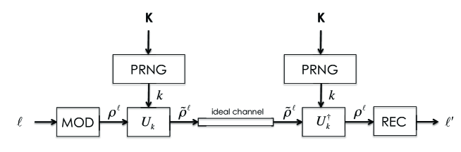
Figure 1: configuration of quantum random cipher system

We briefly explain a configuration of quantum random cipher (Fig. 1). The sender(Alice) modulates her classical message $\ell$ to obtain a signal state $\rho^{\ell}$. Then the signal state is transformed into an encrypted state $\tilde{\rho}^{\ell}$ by a unitary operator $U_{k}$, which is randomly chosen via a running key $k$ generated by using PRNG on a secret key K. We assume the encrypted state $\tilde{\rho}^{\ell}$ is sent through the ideal channel. Since the secret key K, PRNG and map $k\to U_{k}$ are shared by Alice and Bob, Bob can apply the unitary operator $U_{k}^{\dagger}$ to the received state $\tilde{\rho}^{\ell}$ and obtains the signal state $\rho^{\ell}$. Thus Bob can receive a classical message $\ell^{\prime}$ with a very small error by applying the optimum detection to $\rho^{\ell}$. In contrast, Eve does not know the secret key K and hence she must detect encrypted state $\tilde{\rho}^{\ell}$ directly. This makes Eve’s symbol error probability worse than Bob’s one. In the quantum random cipher, a ciphertext is protected against Eve’s attack by a quantum noise. This enables fresh key generation by communication or information theoretic security against known plaintext attack in the symmetric key cipher. So evaluation of Eves’s symbol error probability is essential for security analysis of quantum random cipher.

2.2 Bob’s symbol error probability for PPM signals

We restrict ourselves to the case where $\rho_{\ell}$ is given by the PPM signal $|\Phi_{\ell}\rangle\langle\Phi_{\ell}|$ and each mode in Eq. (1) is from a different time segment. The PPM signals are quantum analog of orthogonal signals in classical communication theory, and error probabilities given by detections for them are summarized in [16]. When the optimum receiver is used, the symbol error probability is [10, 17]

$$P_{B}^{o}=\frac{N-1}{N^{2}}\{[1+(N-1)e^{-S}]^{1/2}-(1-e^{-S})^{1/2}\}^{2}.$$ (5)

When the photon counting receiver is used, the symbol error probability is

$$P_{B}^{c}=(1-1/N)e^{-S},$$ (6)

where error occurs when no photons are found in any of the modes.

Let the signals be transmitted every $T$ seconds. The signal power is $\hbar\omega_{c}{\cal P}=\hbar\omega_{c}S/T$ with an oscillator frequency $\omega_{c}$ and the rate is $R=\ln N/T$ [ebits/sec]. Then it is found that for fixed any values of ${\cal P}$ and $R$ we have $P_{B}^{o}\to 0$ and $P_{B}^{c}\to 0$ as $T\to\infty$. This means that the capacity has an infinite value in both cases. On the other hand, the quasi-classical(homodyne) receiver, cannot achieve an infinite capacity [16]. As clarified later, Eve’s optimum receiver is of such a type, and the capacity takes a finite value. This implies that we can make Eve’s symbol error probability close to $1$ with keeping $P_{B}^{o}$ or $P_{B}^{c}$ close to $0$. The estimation of Eve’s symbol error probability is shown in Section 4.

2.3 Quantum Gaussian Waveform

In order to describe the unitary operator $U_{k}$ in Section 3, we summarize the description of the electromagnetic field generated by a signal source. For simplicity, we use the Holevo’s notations given in the section IV.4 [13]; more realistic ones can be found in [11].

Let us consider the periodic operator-valued function

$$X(t)=\sum_{j=1}^{\infty}\sqrt{\frac{2\pi\hbar\omega_{j}}{T}}\left(a_{j}e^{-i\omega_{j}t}+a_{j}^{\dagger}e^{i\omega_{j}t}\right)\quad t\in[0,T],$$ (7)

where $[0,T]$ is the observation interval, $a^{\dagger}_{j},a_{j}$ are the creation-annihilation operators and $\omega_{j}=2\pi j/T$. We assume the mode $a_{j}$ is described by the Gaussian states

$$\rho_{j}(\alpha_{j})=\frac{1}{\pi N_{j}}\int\exp\left(-\frac{|z-\alpha_{j}|^{2}}{N_{j}}\right)|z\rangle\langle z|d^{2}z$$ (8)

with the first two moments given by

$${\rm Tr}\rho_{j}(\alpha_{j})a_{j} = \alpha_{j},$$ (9)

$${\rm Tr}\rho_{j}(\alpha_{j})a_{j}^{\dagger}a_{j} = N_{j}+|\alpha_{j}|^{2}.$$ (10)

Then the whole process $X(t)$ is characterized by the product Gaussian states $\rho_{\alpha}=\otimes_{j=1}^{\infty}\rho_{j}(\alpha_{j})$, such that

$${\rm Tr}\rho_{\alpha}X(t)=\alpha(t),$$ (11)

$${\rm Tr}\rho_{\alpha}\frac{1}{4\pi}\int_{0}^{T}X(t)^{2}dt=\sum_{j=1}^{\infty}\hbar\omega_{j}(N_{j}+\frac{1}{2})+\frac{1}{4\pi}\int_{0}^{T}\alpha(t)^{2}dt.$$ (12)

Here $\alpha(t)$ is a classical signal for quantum Gaussian channel,

$$\alpha(t)=\sum_{j=1}^{\infty}\sqrt{\frac{2\pi\hbar\omega_{j}}{T}}(\alpha_{j}e^{-i\omega_{j}t}+\bar{\alpha}_{j}e^{i\omega_{j}t}),$$ (13)

where $\bar{\alpha}_{j}$ is a complex conjugate of $\alpha_{j}$.

Now let us rewrite the PPM quantum signal $|\Phi_{\ell}\rangle$ by using the representation of quantum Gaussian waveform. The classical signal corresponding to $|\Phi_{\ell}\rangle$ is given by

$$\alpha^{\ell}(t)=\alpha_{c}(t)\chi_{I_{\ell}}(t)$$ (14)

where

$$\alpha_{c}(t)=\sqrt{\frac{2\pi\hbar\omega_{c}}{T}}\sqrt{NS}(e^{-i\omega_{c}t}+e^{i\omega_{c}t}),$$ (15)

$$\chi_{I_{\ell}}(t)=\left\{\begin{array}[]{ll}1,&t\in I_{\ell}\\ 0,&t\in[0,T]\setminus I_{\ell}\\ \end{array}\right.,$$ (18)

$\omega_{c}=2\pi j_{c}/T$ is a carrier frequency and $I_{\ell}=[(\ell-1)T/N,\ell T/N]$. Assuming the value of $2j_{c}$ is divisible by $N$, we obtain the energy of signal $\alpha^{\ell}$ as

$$\frac{1}{4\pi}\int_{0}^{T}\alpha^{\ell}(t)^{2}dt=\hbar\omega_{c}S.$$ (19)

The Gaussian state corresponding to the classical signal $\alpha^{\ell}(t)$ is given by

$$\rho^{\ell}=\otimes_{j=1}^{\infty}\rho_{j}(\alpha_{j}^{\ell}),\quad\rho_{j}(\alpha_{j}^{\ell})=|\alpha_{j}^{\ell}\rangle\langle\alpha_{j}^{\ell}|,$$ (20)

where we obtain the values of $\alpha_{j}^{\ell}$ from the Fourier series expansion of $\alpha^{\ell}(t)$:

$$\alpha^{\ell}(t)=\sum_{j=1}^{\infty}\sqrt{\frac{2\pi\hbar\omega_{j}}{T}}\left(\alpha_{j}^{\ell}e^{-i\omega_{j}t}+\bar{\alpha}_{j}^{\ell}e^{i\omega_{j}t}\right).$$ (21)

Applying the relation

$$\alpha^{\ell}(t)=\alpha^{1}(t-\frac{\ell-1}{N}T),\quad\ell=1,....,N$$ (22)

to Eq. (21), we have

$$\alpha_{j}^{\ell}=\alpha_{j}^{1}e^{i\omega_{j}(\ell-1)T/N}=\alpha_{j}^{1}e^{i2\pi j(\ell-1)/N}.$$ (23)

3 Phase mask encryption

In this section we introduce an idea of canonical encryption basing on the general theory of Gaussian state [12]. The canonical encryption gives a generalization of encryptions used in the CPPM and phase mask systems. Particularly we are interested in the phase mask encryption, which are formulated in the subsection 3.4. In our phase mask encryption we apply a unitary transformation on a finite number of modes with frequencies $\omega_{j}$ in the vicinity of a nominal carrier frequency $\omega_{c}$, i.e. $j\in J=\{j>0;|\omega_{j}-\omega_{c}|<B\}=\{j_{1},...,j_{M}\}$, although PPM signals are represented by infinite number of modes in the picture of Gaussian waveform. So we may also confine ourselves to a system with a finite number of degrees of freedom in the subsections 3.1, 3.2 and 3.3. Note that the canonical encryption is defined by using Stone-von Neumann theorem, which does not hold for an infinite number of degrees of freedom [18]. From Eqs. (43),(44) and (45) it is found that for an arbitrary small $\epsilon$ there exists $j_{0}>0$ such that $|\alpha_{j}^{\ell}|<\epsilon$ holds for any $j>j_{0}$. So our assumption of finite bandwidth does not affect the security of our system.

3.1 General Definition of Gaussian States

We give a general definition of Gaussian state. In the following superscript $T$ denotes transpose operation for a vector or matrix. Let us consider the Weyl operator for a real vector $z=(z_{j_{1}}^{q},z_{j_{1}}^{p},....,z_{j_{M}}^{q},z_{j_{M}}^{p})^{T}$

$$V(z)=\exp i\sum_{j\in J}(z_{j}^{q}q_{j}+z_{j}^{p}p_{j}),$$ (24)

where

$$\begin{split}q_{j}&=\sqrt{\frac{\hbar}{2\omega_{j}}}(a_{j}+a_{j}^{\dagger})\\ p_{j}&=i\sqrt{\frac{\hbar\omega_{j}}{2}}(a_{j}^{\dagger}-a_{j}),\end{split}$$ (25)

are canonical pairs satisfying the Heisenberg CCR

$$[q_{j},p_{k}]=i\delta_{j,k}I,\quad[q_{j},q_{k}]=[p_{j},p_{k}]=0.$$ (26)

Here $\delta_{j,k}$ takes the value of $1$ when $j=k$ and the value of $0$ otherwise. The Weyl operators $V(z)$ satisfy the Weyl-Segal CCR

$${V}(z){V}(z^{\prime})=\exp\left[\frac{i}{2}\Delta(z,z^{\prime})\right]{V}(z+z^{\prime}),$$ (27)

with $\Delta(z,z^{\prime})=\hbar\sum_{j\in J}(z^{\prime q}_{j}z_{j}^{p}-z_{j}^{q}z^{\prime p}_{j})$. The density operator $\rho$ is called Gaussian if its quantum characteristic function has the form

$${\rm Tr}\rho V(z)=\exp\left[iv^{T}z-\frac{1}{2}z^{T}Az\right],$$ (28)

with mean vector $v$ and correlation matrix $A$. In particular, the Gaussian state $\rho_{\ell}$ given by Eq. (20) has the mean vector

$$v=\Omega_{M}(x_{j_{1}},y_{j_{1}},.....,x_{j_{M}},y_{j_{M}})^{T}$$ (29)

with $\alpha_{j}=x_{j}+iy_{j}$ and

$$\Omega_{M}=\oplus_{m=1}^{M}\left[\begin{array}[]{cc}\sqrt{2\hbar/\omega_{j_{m}}}&0\\ 0&\sqrt{2\hbar\omega_{j_{m}}}\end{array}\right],$$ (30)

and the correlation matrix

$$A_{M}=\oplus_{m=1}^{M}\left[\begin{array}[]{cc}\hbar/2\omega_{j_{m}}&0\\ 0&\hbar\omega_{j_{m}}/2\end{array}\right]=\frac{1}{4}\Omega_{M}^{2}.$$ (31)

3.2 Symplectic Transformation

The transformation $L:{\mathbb{R}}^{2M}\to{\mathbb{R}}^{2M}$ is called symplectic, when the corresponding Weyl operators $\tilde{V}(z)=V(L^{T}z)$ satisfies the Weyl-Segal CCR (27). We denote the totality of symplectic transformation by ${\rm Sp}(M,{\mathbb{R}})$. It follows from Stone-von Neumann theorem that there exists the unitary operator $U$ satisfying

$$V(L^{T}z)=U^{\dagger}V(z)U$$ (32)

for any $L\in{\rm Sp}(M,{\mathbb{R}})$. We call such derived operator $U$ the unitary operator associated with symplectic transformation $L$. The characteristic function of $\tilde{\rho}^{\ell}=U\rho^{\ell}U^{\dagger}$ is given by

$$\begin{split}{\rm Tr}\tilde{\rho}^{\ell}V(z)=&{\rm Tr}\rho^{\ell}U^{\dagger}V(z)U\\ =&{\rm Tr}\rho^{\ell}V(L^{T}z)=\exp\left[i(Lv)^{T}z-\frac{1}{2}z^{T}LA_{M}L^{T}z\right]\end{split}$$ (33)

In the following we confine ourselves to the Gaussian state $\rho_{\ell}$ given by Eq. (20), and our interest is devoted to the case where the state $\tilde{\rho}^{\ell}$ has the form of $\otimes_{j\in J}|\tilde{\alpha}_{j}^{\ell}\rangle\langle\tilde{\alpha}_{j}^{\ell}|$. Then the symplectic transformation should satisfy the condition $LA_{M}L^{T}=A_{M}$, which means

$$\Omega_{M}^{-1}L\Omega_{M}(\Omega_{M}^{-1}L\Omega_{M})^{T}=I_{2M}$$ (34)

i.e.

$$\Omega_{M}^{-1}L\Omega_{M}\in{\rm O}(2M)\cap{\rm Sp}(M,{\mathbb{R}})\cong{\rm U}(M)$$ (35)

where ${\rm U}(M)$ denotes the totality of $M\times M$ unitary matrices and ${\rm O}(2M)$ the totality of $2M\times 2M$ orthogonal matrices.

3.3 Canonical Encryption

In the canonical encryption, we encrypt the message using unitary operator $U_{k}$ associated with $L_{k}$ satisfying Eq. (35). In the isomorphism ${\rm O}(2M)\cap{\rm Sp}(M,{\mathbb{R}})\cong{\rm U}(M)$, an element of ${\rm O}(2M)\cap{\rm Sp}(M,{\mathbb{R}})$,

$$\begin{pmatrix}r_{11}R(\theta_{11})&\cdots&r_{1M}R(\theta_{1M})\\ \vdots&\ddots&\vdots\\ r_{M1}R(\theta_{M1})&\cdots&r_{MM}R(\theta_{MM})\\ \end{pmatrix},$$ (36)

corresponds to

$$\begin{pmatrix}r_{11}e^{i\theta_{11}}&\cdots&r_{1M}e^{\theta_{1M}}\\ \vdots&\ddots&\vdots\\ r_{M1}e^{i\theta_{M1}}&\cdots&r_{MM}e^{\theta_{MM}}\\ \end{pmatrix}\in{\rm U}(M).$$ (37)

with $r_{ij}\in{\mathbb{R}}$ and rotation matrices $R(\theta_{ij})$. We denote the unitary matrix corresponding to $\Omega_{M}^{-1}L_{k}\Omega_{M}$ by $U_{L_{k}}$. Then we can find the Gaussian state $\rho^{\ell}=\otimes_{j\in J}\rho_{j}(\alpha_{j}^{\ell})$ is encrypted into

$$\tilde{\rho}^{\ell}=\otimes_{j\in J}\rho_{j}(\beta_{j}^{\ell})$$ (38)

with

$$(\beta_{j_{1}}^{\ell},.....,\beta_{j_{M}}^{\ell})^{T}=U_{L_{k}}(\alpha_{j_{1}}^{\ell},.....,\alpha_{j_{M}}^{\ell})^{T}.$$ (39)

Note that the number $M$ of encrypted modes can be taken larger than the number $N$ of pulse positions unlike the case of CPPM with the encryption (2).

3.4 Phase Mask Encryption

We consider an example of the canonical encryption. If $r_{ij}=\delta_{ij}$ holds for $i,j=1,...,M$ in the matrix (37), the canonical encryption is called a phase mask encryption and the matrix (37) is denoted by $U(\theta_{11},...,\theta_{MM})$. We assume $N$ is a prime number. Then in the right-hand side of Eq. (23), we have

$$\{e^{i2\pi j(\ell-1)/N};\ell=1,...,N\}=\{e^{i2\pi n/N};n=1,...,N\},$$ (40)

if the value of $j$ is not divisible by $N$. So it is natural to consider the phase mask encryption given by

$$U_{L_{k}}=U(2\pi k_{1}/N^{\prime},....,2\pi k_{M}/N^{\prime}),$$ (41)

where $N^{\prime}$ is a multiple of $N$ and $k=(k_{1},...,k_{M})$ with $0\leq k_{m}<N^{\prime}$ is a key generated from PRNG. Then each $\beta_{j_{m}}^{\ell}$ in Eq. (39) takes values of the form

$$\alpha^{1}_{j_{m}}e^{i2\pi n^{\prime}/N^{\prime}},\quad n^{\prime}=1,...,N^{\prime}.$$ (42)

In particular, when $N=2,M=1$, this cryptosystem is equivalent to the $\alpha\eta$ cryptosystem with PSK modulation. In Fig. 2, we show an example of signal configuration of $\alpha_{j_{m}}^{\ell},\beta_{j_{m}}^{\ell}$ in the case of $N=3,N^{\prime}=9,M=2$. The black points in the figure represent the parameters $\alpha_{j_{m}}^{\ell}$ for the original set of signal states $\{\rho^{\ell},\ell=1,2,3\}$. By the phase mask encryption with $N^{\prime}/N=3$ we can use $3$ types of sets of signal states. In general, the condition $p=N^{\prime}/N$ gives $p$ types of sets of signal states.

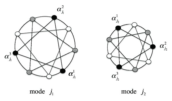
Figure 2: Signal configuration of a phase mask modulation ($N=3,N^{\prime}=9,M=2$)

Figure 3: Example of a signal transformed by the phase mask encryption

Let us obtain Fourier series for the signal $\alpha^{\ell}(t)$. For simplicity we use a usual expression of Fourier series instead of Eq. (21):

$$\alpha^{\ell}(t)=\sum_{j=-\infty}^{\infty}c_{j}^{\ell}e^{i\omega_{j}t},$$ (43)

where $c^{\ell}_{j}=\sqrt{2\pi\hbar\omega_{j}/T}\bar{\alpha}^{\ell}_{j}$ and $c^{\ell}_{-j}=\sqrt{2\pi\hbar\omega_{j}/T}{\alpha}^{\ell}_{j}$ for $j>0$. Then coefficients $c_{j}^{\ell}$ are computed as

$$c_{j}^{\ell}=\sqrt{\frac{2\pi\hbar\omega_{c}}{T}}\sqrt{NS}(d_{j+j_{c}}^{\ell}+d_{j-j_{c}}^{\ell}),$$ (44)

where $d_{j}^{\ell}$ are Fourier coefficients of $\chi_{I_{\ell}}(t)$:

$$d_{j}^{\ell}=\frac{1}{N}e^{-i\pi j(2\ell-1)/N}{\rm sinc}\frac{j}{N}\pi,$$ (45)

with ${\rm sinc}x=\sin x/x$. Fig. 3 shows how $\chi_{I_{\ell}(t)}$ is transformed by the phase mask encryption in a realistic setting, where the carrier frequency is $f_{c}=\omega_{c}/2\pi=200$[THz], the frequency resolution $1/T=10$[MHz], the bandwidth is limited to $1$[GHz] (i.e. number of modes $M$ is $100$), $N=97$ and $N^{\prime}=9700$. In this case the transmission rate is $R=\ln N/T=45.7$ [M ebits/sec].

Since both of PPM signal and the one encrypted by a phase mask do have most of their energy at frequencies included in the main lobe of sinc function, effective modes for encryption are restricted to those frequencies. So in the case of phase mask encryption we cannot set the value of $M$ independently of $N$; when we use the modes $j$ satisfying $(j-j_{c})\pi/N<\pi$, $M=2N-1$.

4 Evaluation of Eve’s symbol error probability

4.1 Heterodyne attack

Here we consider the phase mask encryption described in Sec. 3.4, avoiding complicated notations. We can apply the same discussion to a general case. Eve tries to estimate the classical message $\ell$ (or the secret key) from her observation of encrypted states

$${\rho}(n^{\prime})=\otimes_{j\in J}\rho_{j}(\alpha_{j}^{1}e^{i2\pi n^{\prime}_{j}/N^{\prime}}),$$ (46)

where $J=\{j_{1},...,j_{M}\}$ and $n^{\prime}=(n^{\prime}_{j_{1}},...,n^{\prime}_{j_{M}})$ with integers $1\leq n^{\prime}_{j_{m}}\leq N^{\prime}$. Then the error probability of her observation is given by

$$P=1-\sum_{n^{\prime}}{\rm Tr}{\rm\Pi}_{n^{\prime}}^{o}\rho(n^{\prime}),$$ (47)

where $\{{\rm\Pi}_{n^{\prime}}^{o}\}$ is a positive operator valued measure (POVM) describing Eve’s optimum measurement, and it goes to $1$ as $N^{\prime}\to\infty$. This shows that Eve cannot estimate the message $\ell$ correctly for enough large $N^{\prime}$. However it cannot ensure that our proposed system exceeds the Shannon limit. In order to show it, we have to evaluate Eve’s symbol error probability $P_{E}$ under assumption that she can get the secret key K after obtaining cipher text by the measurement $\{{\rm\Pi}_{n^{\prime}}^{o}\}$.

In the following we evaluate Eve’s symbol error probability $P_{E}$ under the above assumption. In addition we may assume that she uses the following measurement on the modes $J=\{j_{1},...,j_{M}\}$ of the states $\rho(n^{\prime})$:

$$X(\vec{\beta}^{\prime})=\otimes_{j\in J}\frac{|\beta^{\prime}_{j}\rangle\langle\beta^{\prime}_{j}|}{\pi},$$ (48)

with $\vec{\beta}^{\prime}=(\beta^{\prime}_{j_{1}},...,\beta^{\prime}_{j_{M}})$. Note that a measurement described by Eq. (48) is realized by the heterodyne detection when the bandwidth $2B$ is enough small [8]. Then Eve guesses a value of $n^{\prime}$ from the result $\vec{\beta}^{\prime}$of the measurement by using a function decided beforehand $g:\vec{\beta}^{\prime}\to n^{\prime}$. This gives a POVM $\{{\rm\Pi}_{n^{\prime}}\}$ describing a suboptimal measurement, where

$${\rm\Pi}_{n^{\prime}}=\int_{g^{-1}(n^{\prime})}X(\vec{\beta}^{\prime})d\vec{\beta}^{\prime}.$$ (49)

Here Eve’s symbol error probability $P_{E}$ is very little worse than that obtained by the optimum measurement$\{{\rm\Pi}_{n^{\prime}}^{o}\}$, because Eve does not know the secret key K and there are phase (and amplitude) uncertainties for each $\beta_{j}^{\ell}$, $j\in J$ in Eq. (38). Moreover we introduce a lower bound $\bar{P}_{E}$ of ${P}_{E}$ by assuming Eve can know the secret key after her obtaining an electrical signal by the measurement (48). In this case Eve can discriminate plaintext directly as explained below. Such a condition is too advantageous to Eve and hence $\bar{P}_{E}$ only gives a very loose lower bound of $P_{E}$. However we have to confine ourselves to evaluating the lower bound $\bar{P}_{E}$ because of a difficulty in computing $P_{E}$.

When a message $\ell$ is transmitted, Eve obtains the signal described as a stochastic process

$$\beta_{E}^{\ell}(t)=\sum_{j\in J}\sqrt{\frac{2\pi\hbar\omega_{j}}{T}}\left({\beta^{\prime}_{j}}^{\ell}e^{-i\omega_{j}t}+\bar{\beta^{\prime}_{j}}^{\ell}e^{i\omega_{j}t}\right)$$ (50)

as a result of her measurement (48). Here $\vec{\beta}^{\prime\ell}=(\beta^{\prime\ell}_{j_{1}},....,\beta^{\prime\ell}_{j_{M}})^{T}$ is a random vector subject to the probability density function

$$P_{\tilde{\rho}^{\ell}}(\vec{\beta}^{\prime\ell})={\rm Tr}\tilde{\rho}^{\ell}X(\vec{\beta}^{\prime\ell}).$$ (51)

In our setting, Eve knows the secret key ${\bf K}$ after her measurement. So using the adjoint operator $U^{*}_{L_{k}}$ of $U_{L_{k}}$ she can compute $\vec{\alpha}^{\prime\ell}=U^{*}_{L_{k}}\vec{\beta}^{\prime\ell}=(\alpha^{\prime\ell}_{j_{1}},...,\alpha^{\prime\ell}_{j_{M}})^{T}$, which is a random vector whose probability density is given by $P_{\tilde{\rho}^{\ell}}(U_{L_{k}}\vec{\alpha}^{\prime\ell})=P_{\tilde{\rho}^{\ell}}(\vec{\beta}^{\prime\ell})$. From Eq. (51), we have

$$\begin{split}P_{\tilde{\rho}^{\ell}}(\vec{\beta}^{\prime\ell})=&{\rm Tr}U_{k}\rho^{\ell}U_{k}^{\dagger}X(\vec{\beta}^{\prime\ell})\\ =&{\rm Tr}\rho^{\ell}U_{k}^{\dagger}X(\vec{\beta}^{\prime\ell})U_{k}\\ =&{\rm Tr}\rho^{\ell}X(\vec{\alpha}^{\prime\ell})\end{split}$$ (52)

This shows that the random vector $\vec{\alpha}^{\prime\ell}$ obeys to the probability density function ${\rm Tr}\rho^{\ell}X(\vec{\alpha}^{\prime\ell})$, i.e. $\alpha^{\prime\ell}_{j_{m}}$ is a complex random variable with the mean $\alpha^{\ell}_{j_{m}}$ and the variance $1/2$. As a result we can find that Eve obtains the signal

$$\alpha_{E}^{\ell}(t)=\sum_{j\in J}\sqrt{\frac{2\pi\hbar\omega_{j}}{T}}\left(\alpha^{\prime\ell}_{j}e^{-i\omega_{j}t}+\bar{\alpha}^{\prime\ell}_{j}e^{i\omega_{j}t}\right),$$ (53)

where random variables $\alpha^{\prime\ell}_{j}$ have the mean $\alpha^{\ell}_{j}$ and the variance $1/2$.

4.2 Eve’s symbol error probability

We evaluate Eve’s symbol error probability, when she tries to estimate the value of $\ell$ from the signal $\alpha^{\ell}_{E}(t)$. For the sake of brevity, we rewrite $\alpha^{\ell}(t)$ and $\alpha^{\ell}_{E}(t)$ as

$$\begin{split}\alpha^{\ell}(t)&=2{\rm Re}\sum_{j=1}^{\infty}\sqrt{\hbar\omega_{j}}\alpha^{\ell}_{j}\xi_{j}(t),\\ \alpha^{\ell}_{E}(t)&=2{\rm Re}\sum_{j\in J}\sqrt{\hbar\omega_{j}}\alpha^{\prime\ell}_{j}\xi_{j}(t),\\ \xi_{j}(t)&=\sqrt{\frac{2\pi}{T}}e^{-i\omega_{j}t},\end{split}$$ (54)

where we denote real part of complex number by ${\rm Re}z$. Let us introduce an inner product as

$$\langle\psi,\varphi\rangle=\frac{1}{4\pi}\int_{0}^{T}{\psi}(t)\varphi(t)dt.$$ (55)

We also use this notation for a complex function and have $\langle\xi_{j},\xi_{k}\rangle=\langle\bar{\xi}_{j},\bar{\xi}_{k}\rangle=0$ and $\langle\bar{\xi}_{j},\xi_{k}\rangle=\langle{\xi}_{j},\bar{\xi}_{k}\rangle=\delta_{j,k}$. By definition the signals $\alpha^{\ell}(t)$ are orthogonal to each other and hence we can constitute the orthonormal basis

$$\psi_{\ell}(t)\equiv\alpha^{\ell}(t)/\parallel\alpha^{\ell}\parallel,\quad\ell=1,...,N,$$ (56)

where the norm is given by

$$\parallel\alpha^{\ell}\parallel=\sqrt{\langle\alpha^{\ell},\alpha^{\ell}\rangle}=\sqrt{\sum_{j=1}^{\infty}\hbar\omega_{j}|\alpha_{j}^{\ell}|^{2}}.$$ (57)

From Eq. (19) we have another expression for the norm of $\alpha^{\ell}$ as

$$\parallel\alpha^{\ell}\parallel^{2}={\hbar\omega_{c}S},$$ (58)

which shows that $\parallel\alpha^{\ell}\parallel$ has a fixed value for any $\ell$. With the basis $\{\psi_{\ell}\}$, we represent the signal $\alpha^{\ell}(t)$ as the vector $(0,...,0,\sqrt{\hbar\omega_{c}S},0,...,0),$ whose elements take the value $0$ except the $\ell$th element.

Let us obtain the vector representation of $\alpha^{\ell}_{E}(t)$. Its $k$th element is computed as

$$\langle\psi_{k},\alpha^{\ell}_{E}\rangle=\langle\psi_{k},2{\rm Re}\sum_{j\in J}\sqrt{\hbar\omega_{j}}\alpha_{j}^{\ell}\xi_{j}\rangle+\langle\psi_{k},2{\rm Re}\sum_{j\in J}\sqrt{\hbar\omega_{j}}z_{j}\xi_{j}\rangle,$$ (59)

where $z_{j}$ is a complex random variable with the mean $0$ and the variance $1/2$. Here the second term is computed as

$$\frac{{\rm Re}\sum_{j\in J}\hbar\omega_{j}\bar{\alpha}_{j}^{\ell}z_{j}}{\parallel\alpha_{\ell}\parallel},$$ (60)

which has the variance

$$\hbar\omega_{c}\frac{D}{2}$$ (61)

with

$$D=\frac{\sum_{j\in J}|\alpha_{j}^{\ell}|^{2}\omega_{j}^{2}}{\sum_{j=1}^{\infty}|\alpha_{j}^{\ell}|^{2}\omega_{j}\omega_{c}}.$$ (62)

Assuming that the signals $\alpha^{\ell}$ have most of their energy at frequencies $\omega_{j}$ ($j\in J$) and $\omega_{c}>>1/(T/N)$, we have the approximations

$$\alpha^{\ell}(t)\approx 2{\rm Re}\sum_{j\in J}\sqrt{\hbar\omega_{j}}\alpha_{j}^{\ell}\xi_{j}(t)$$ (63)

and $d_{j+j_{c}}^{\ell}\approx 0$ in Eq. (44). Then it holds

$$\langle\psi_{k},2{\rm Re}\sum_{j\in J}\sqrt{\hbar\omega_{j}}\alpha_{j}^{\ell}\xi_{j}\rangle\approx\langle\psi_{k},\alpha^{\ell}\rangle=\delta_{k\ell}\sqrt{\hbar\omega_{c}S},$$ (64)

and

$$\begin{split}D&\approx\frac{\sum_{j\in J}|\alpha_{j}^{\ell}|^{2}\omega_{j}^{2}}{\sum_{j\in J}|\alpha_{j}^{\ell}|^{2}\omega_{j}\omega_{c}}\approx\frac{\sum_{j\in J}(\omega_{c}NS/\omega_{j})|d_{j-j_{c}}^{\ell}|^{2}\omega_{j}^{2}}{\sum_{j\in J}(\omega_{c}NS/\omega_{j})|d_{j-j_{c}}^{\ell}|^{2}\omega_{j}\omega_{c}}\\ &=\frac{\sum_{j\in J^{\prime}}|d_{j}^{\ell}|^{2}\omega_{j+j_{c}}}{\sum_{j\in J^{\prime}}|d_{j}^{\ell}|^{2}\omega_{c}}=\frac{\sum_{j\in J^{\prime}}|d_{j}^{\ell}|^{2}(j+j_{c})}{\sum_{j\in J^{\prime}}|d_{j}^{\ell}|^{2}j_{c}}\geq 1,\end{split}$$ (65)

with $J^{\prime}=\{j;|\omega_{j+j_{c}}-\omega_{c}|<B,j+j_{c}>0\}$, $\omega_{j}=2\pi j/T$ and $\omega_{c}=\omega_{j_{c}}=2\pi j_{c}/T$. The last inequality in Eq. (65) is shown by using $|d_{j}^{\ell}|=|d_{-j}^{\ell}|$ and it becomes the equality in the usual case, where $\pm j+j_{c}$ has a positive value for any $j\in J^{\prime}$. Thus we find the vector representation of $\alpha_{E}^{\ell}$ is given by $(w_{1},w_{2},..,w_{\ell-1},\sqrt{\hbar\omega_{c}S}+w_{\ell},w_{\ell+1},...,w_{N}),$ where $w_{k}$ is a complex random variable with the mean $0$ and the variance $\hbar\omega_{c}D/2$. In the following for simplicity we consider the equivalent situation where the vector representation is given by $(y_{1},...,y_{\ell},...,y_{N})=(w_{1},w_{2},..,w_{\ell-1},A+w_{\ell},w_{\ell+1},...,w_{N})$ with $A^{2}=2S/D$ and $w_{k}$ has the mean $0$ and the variance $1$.

In our setting Eve uses maximum-likelihood decoding, where Eve picks the element $m$ for which $y_{m}$ is largest. According to [15], when message $\ell$ is sent Eve’s symbol error probability is given by

$$\bar{P}_{E}=\int_{-\infty}^{\infty}\frac{1}{\sqrt{2\pi}}\exp\left[-\frac{(y_{\ell}-A)^{2}}{2}\right]Q_{N}(y_{\ell})dy_{\ell},$$ (66)

where $Q_{N}(y_{\ell})$ is the probability that $y_{\ell^{\prime}}\geq y_{\ell}$ for some $\ell^{\prime}\neq\ell$:

$$\begin{split}Q_{N}(y)&=1-[\Phi(y)]^{N-1},\\ \Phi(y)&=\frac{1}{\sqrt{2\pi}}\int_{-\infty}^{y}\exp(-v^{2}/2)dv.\end{split}$$ (67)

We remark that $\bar{P}_{E}$ does not depend on $\ell$. Recall the signals have duration $T$ and power $\hbar\omega_{c}{\cal P}=\hbar\omega_{c}S/T$. Then

$$A=\sqrt{2S/D}=\sqrt{2T{\cal P}/D}=\sqrt{2TC_{E}},$$ (68)

with $C_{E}={\cal P}/D$ holds and the transmission rate is given by

$$R=\frac{\ln N}{T}\quad{\rm[ebits/sec]}.$$ (69)

Let us consider a Gaussian channel, where the input power is constrained to $\hbar\omega_{c}{\cal P}$, the Gaussian noise has the variance $\hbar\omega_{c}D/2$ and the number of degrees of freedom is unconstrained. Then its capacity per unit time is given by $C_{E}={\cal P}/D$[ebits/sec] (Corollary of Theorem 8.2.1 in [15]). In [15], it is shown that $\bar{P}_{E}\to 0$ as $T\to\infty$ if $R<C_{E}$ by estimating lower and upper bounds of $\bar{P}_{E}$. We show $\bar{P}_{E}\to 1$ as $T\to\infty$ if $R>C_{E}$ by obtaining a lower bound of $\bar{P}_{E}$. We start with the inequalities used in [15]:

$$\begin{split}\bar{P}_{E}&\geq\int_{-\infty}^{y}\frac{1}{\sqrt{2\pi}}\exp\left[-\frac{(y_{\ell}-A)^{2}}{2}\right]Q_{N}(y_{\ell})dy_{\ell}\\ &\geq Q_{N}(y)\Phi(y-A),\end{split}$$ (70)

where $y$ is an arbitrary number and $Q_{N}(y)\Phi(y-A)$ is the probability that $y_{\ell}<y$ and $y_{\ell^{\prime}}\geq y$ for some $\ell^{\prime}$. We can find lower bounds of $Q(y)$ and $\Phi(y-A)$ by using the standard inequalities on the Gaussian distribution for $y>0$ [14]:

$$\left(\frac{1}{y}-\frac{1}{y^{3}}\right)\frac{\exp(-y^{2}/2)}{\sqrt{2\pi}}<\Phi(-y)<\frac{1}{y\sqrt{2\pi}}\exp(-y^{2}/2).$$ (71)

That is, we have

$$\begin{split}Q_{N}(y)&=1-[1-\Phi(-y)]^{N-1}=1-\exp[(N-1)\ln(1-\Phi(-y))]\\ &\geq 1-\exp[-(N-1)\Phi(-y)]\\ &\geq 1-\exp\left[-(N-1)\left(\frac{1}{y}-\frac{1}{y^{3}}\right)\frac{\exp(-y^{2}/2)}{\sqrt{2\pi}}\right],\end{split}$$ (72)

and for $y>A$

$$\Phi(y-A)=1-\Phi(-(y-A))\geq 1-\frac{1}{\sqrt{2\pi}(y-A)}\exp(-(y-A)^{2}/2).$$ (73)

Putting

$$y=\sqrt{f\ln N}>A,$$ (74)

we obtain the lower bound of $\bar{P}_{E}$ as

$$\begin{split}\bar{P}_{E}\geq&\left(1-\exp\left[-\left(1-\frac{1}{N}\right)\left(1-\frac{1}{f\ln N}\right)\sqrt{\frac{N^{2-f}}{2\pi f\ln N}}\right]\right)\\ &\times\left(1-\frac{1}{\sqrt{2\pi}(\sqrt{f\ln N}-A)}\exp\left[-\frac{(\sqrt{f\ln N}-A)^{2}}{2}\right]\right)\\ =&\left(1-\exp\left[-\left(1-e^{-RT}\right)\left(1-\frac{1}{fRT}\right)\sqrt{\frac{\exp({(2-f)RT})}{2\pi fRT}}\right]\right)\\ &\times\left(1-\frac{1}{\sqrt{2\pi T}(\sqrt{fR}-\sqrt{2C_{E}})}\exp\left[-\frac{(\sqrt{fR}-\sqrt{2C_{E}})^{2}T}{2}\right]\right).\end{split}$$ (75)

Here $f$ is an arbitrary positive number satisfying the inequality $\sqrt{f\ln N}>A$, which is rewritten by using $A=\sqrt{2TC_{E}}$ and $N=e^{RT}$ as

$$f>\frac{2C_{E}}{R}.$$ (76)

When it holds

$$C_{E}<R,$$ (77)

we can find a value of $f$ satisfying $f<2$ and the inequality (76). This shows $\bar{P}_{E}\to 1$ as $T\to\infty$. Putting $\bar{p}_{1}=1-\bar{P}_{E}$, from Eq. (75) we obtain a lower bound for an exponent of $\bar{p}_{1}$ as

$$E_{s}(R)=\lim_{T\to\infty}\left(-\frac{\ln\bar{p}_{1}}{T}\right)\geq\frac{(\sqrt{fR}-\sqrt{2C_{E}})^{2}}{2}.$$ (78)

Considering $f$ can take any value of $2C_{E}/R<f<2$, we have

$$E_{s}(R)\geq{(\sqrt{R}-\sqrt{C_{E}})^{2}}.$$ (79)

When $T$ is large enough, $\bar{P}_{E}$ is approximated and lower bounded as

$$\bar{P}_{E}\approx 1-e^{-E_{s}(R)T}\geq 1-e^{-(\sqrt{R}-\sqrt{C_{E}})^{2}T}.$$ (80)

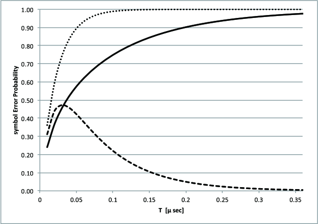
Figure 4: Error probabilities of Bob and Eve with respect to signal duration $T$. Eve’s symbol error probability $\bar{P}_{E}$ under the assumption that she can know the secret key after her measurement is plotted by the real line and Bob’s symbol error probability $P_{B}^{c}$ the broken line. The dot line represents the error probability $1-1/N$ in the case where a message $\ell$ is randomly chosen from $N=e^{RT}$ messages.

N	2	$2^{2}$	$2^{4}$	$2^{6}$	$2^{8}$	$2^{10}$	$2^{12}$	$2^{14}$	$2^{18}$	$2^{22}$
T[$\mu$sec]	0.015	0.031	0.062	0.092	0.12	0.15	0.18	0.21	0.28	0.34

Table 1: Relation between number of pulse positions and signal duration $T$ for the transmission rate $R=45$ [M ebits/sec].

Fig. 4 gives graphs of error probabilities of Bob and Eve for the transmission rate $R=45$ [M ebits/sec], $C_{E}=15$ [M ebits/sec] and $D=1$. In the graph the broken line represents the symbol error probability $P_{B}^{c}$ of Bob achieved by the photon counting receiver, the solid line the lower bound $\bar{P}_{E}$ of Eve’s symbol error probability $P_{E}$, the dot line its upper bound $1-1/N$, which gives the error probability when a message $\ell$ is randomly chosen from $N$ messages. The symbol error probability $\bar{P}_{E}$ is computed numerically from Eq. (66) without using the lower bound. Note that $P_{B}^{c}$ has a peak at $T=(\ln(1+R/C_{E}))/R=0.031$ [$\mu$ sec] and takes a value of $4.52\times 10^{-3}$ at $T=0.36$ [$\mu$ sec]. Here the value of $C_{E}={\cal P}$ is fixed and hence the pulse energy $S=C_{E}T$ increases as $T$ does. So $e^{-S}$, which represents the probability that no photons are found in any of the modes, decreases as $T$ increases. On the other hand, when any photon is not found, we have to guess a pulse position randomly. The error probability for such a random decision, which is given by $1-1/N=1-e^{-RT}$ in Eq. (6), increases as $T$ does. This is why the graph of $P_{B}^{c}=(1-1/N)e^{-S}$ has a peak

The number $N$ of pulse positions is an important parameter to check feasibility of the system. Table 1 shows a relation between $N$ and duration time $T$ for the transmission rate $R=45$ [M ebits/sec]. By using the relations $S=TC_{E}$ and $\ln N=TR$, Eq. (80) and the condition (77) for it can be respectively rewritten as

$$\bar{P}_{E}\geq 1-e^{-(\sqrt{\ln N}-\sqrt{S})^{2}}$$ (81)

and

$$e^{S}<N.$$ (82)

Fixing the value of $E$, we find that the error probabilities $\bar{P}_{E}$, $P_{B}^{o}$ and $P_{B}^{c}$ are determined by the values of $TC_{E}$, $TR$. This means that for an arbitrary number $g>0$, $T=(1/g)T_{0}$, $C_{E}=gC_{E,0}$ and $R=gR_{0}$ give the same value of the error probabilities. On the other hand, the pulse duration

$$\Delta T=\frac{T}{e^{RT}}=\frac{1}{g}\frac{T_{0}}{e^{R_{0}T_{0}}}$$ (83)

takes a smaller value as $g$ (or $R$) takes a larger value.

We remark on the relation between the present system and the CPPM system with the encryption (2). For the latter system we can obtain a lower bound $\bar{P}^{\prime}_{E}$ of symbol error probability, assuming that Eve employs a heterodyne detection on $\alpha_{\ell,n}^{k}$ in Eq. (2) and after her measurement she can get the secret key K [3]. Then it is found that the following equation holds approximately

$$\bar{P}^{\prime}_{E}=\bar{P}_{E}.$$ (84)

Here rigorously speaking it holds that $\bar{P}_{E}>\bar{P}^{\prime}_{E}$ when $D>1$ in Eq. (65), but in a natural setting we have $D\approx 1$ and we may say Eq.(84) holds.

5 Conclusions

We have formulated a security evaluation of CPPM type of quantum random cipher in terms of quantum Gaussian waveform, and have given the mathematical derivation process of the lower bound of Eve’s symbol error probability under the assumption that the secret key is given to Eve after her heterodyne measurement. This model means that Eve can try to discriminate directly plaintext instead of ciphertext after heterodyne measurement. Thus, this ensures a security level being beyond the Shannon limit under stronger condition than in the case that Eve uses the secret key after discrimination of ciphertext based on her heterodyne measurement. We will report a basic experiment for the latter case in the subsequent papers.

References

- [1] O.Hirota, M.Sohma, M.Fuse, and K.Kato, ”Quantum stream cipher by Yuen 2000 protocol: Design and experiment by intensity modulation scheme”, Physical Review A vol-72, 022335 (2005)
- [2] O.Hirota, ”Practical security analysis of quantum stream cipher by Yuen 2000 protocol”, Physical Review A, vol-76, 032307 (2007)
- [3] M. Sohma and O. Hirota, ”Coherent pulse position modulation quantum cipher supported by secret key”, Tamagawa University Quantum ICT Bulletin, Vol.1 No.1,15-19 (2011)
- [4] O.Hirota, ”Everlasting Security by cipher exceeding the Shannon limit of cryptography”, The 29th Symposium on Cryptography and Information Security (2012)
- [5] G.A.Borbosa, E.Corndorf, G.S.Kanter, P.Kumar, and H.P.Yuen, ”Secure communication using mesoscopic coherent states”, Physical Review Letters, vol-90, 227901 (2003)
- [6] H. P. Yuen, ”Key generation: Foundation and a new quantum approach”, IEEE. J. Selected topics in Quantum Electronics, vol.15, no.6,pp. 1630-1645 (2009)
- [7] H.P.Yuen,R.Nair, E.Corndorf, G.S.Kanter, and P.Kumar, ”Quantum Noise Randomized Ciphers”, Quantum Information and Computation, vol-8, p561 (2006)
- [8] H. P. Yuen, J. H. Shapiro, ”Optical Communication with Two-Photon Coherent States-Part III:Quantum Measurements Realizable with Photoemissive Detectors” , IEEE Trans. on Information Theory, vol. IT-26, no.1, pp. 78-92 (1980)
- [9] H. P. Yuen, ”Quantum Cryptography QKD and KCQ”, presented at Tamagawa University, Japan, June 15th (2011)
- [10] H. P.Yuen, R.S. Kennedy and M. Lax, ”Optimum testing of multiple hypotheses in quantum detection theory”, IEEE Trans. on Information Theory IT-21, pp.125-134 (1975).
- [11] H. P. Yuen, J. H. Shapiro, ”Optical Communication with Two-Photon Coherent States-PartI:Quantum-State Propagation and Quantum-Noise Reduction”, IEEE Trans. on Information Theory, vol. IT-24, no.6, pp. 657-668 (1978)
- [12] A. S. Holevo, ”Probabilistic and Statistical Aspect of Quantum Theory”, North-Holland (1982)
- [13] A. S. Holevo, ”Coding Theorems for Quantum Channels”, Tamagawa University Research Review, vol.4 (1998)
- [14] W. Feller, ”An Introduction to Probability Theory and Its Applications Vol. 1 (VII.1)”, John Wiley & Sons (1968)
- [15] R. G. Gallager, ”Information Theory and Reliable Communication”, John Wiley & Sons (1968)
- [16] C. W. Helstrom, ”Quantum Detection and Estimation Theory”, Academic Press (1976)
- [17] C. W. Helstrom, ”Capacity of the Pure-State Quantum Channel”, Proceedings of the IEEE 62, pp.139-140 (1974)
- [18] E.E. Segal, ”Mathematical problems of relativistic physics”, AMS, Providence, RI (1963)