Coherent quantum dynamics in steady-state manifolds of strongly dissipative systems

Abstract

It has been recently realized that dissipative processes can be harnessed and exploited to the end of coherent quantum control and information processing. In this spirit we consider strongly dissipative quantum systems admitting a non-trivial manifold of steady states. We show how one can enact adiabatic coherent unitary manipulations e.g., quantum logical gates, inside this steady-state manifold by adding a weak, time-rescaled, Hamiltonian term into the system’s Liouvillian. The effective long-time dynamics is governed by a projected Hamiltonian which results from the interplay between the weak unitary control and the fast relaxation process. The leakage outside the steady-state manifold entailed by the Hamiltonian term is suppressed by an environment-induced symmetrization of the dynamics. We present applications to quantum-computation in decoherence-free subspaces and noiseless subsystems and numerical analysis of non-adiabatic errors.

Introduction:–  Weak coupling to the environmental degrees of freedom is often regarded as one of the essential prerequisites for realizing quantum information processing. In fact decoherence and dissipation generally spoil the unitary character of the quantum dynamics and induce errors into the computational process. In order to overcome such an obstacle a variety of techniques have been devised including quantum error correction QEC , decoherence-free subspaces (DFSs) DFS ; DFS-exp and noiseless subsystems (NSs) NS ; NS-exp . However, it has been recently realized that dissipation and decoherence may even play a positive role to the aim of coherent quantum manipulations. Indeed, it has been shown that, properly engineered, dissipative dynamics can in principle be tailored to enact quantum information primitives such as quantum state preparation kastoryano2011dissipative , quantum simulation barreiro2011open ; gauge and computation verstraete2009quantum .

In this Letter we investigate the regime where the coupling of the system to the environment is very strong and the open system dynamics admits a non-trivial steady state manifold (SSM). We will show how, in the long time limit, unitary manipulations e.g., quantum gates, inside the SSM can be enacted by adding a time-rescaled Hamiltonian acting on the system only. This coherent dynamics is governed by a sort of projected Hamiltonian which results from the non-trivial interplay between the weak unitary control term and the strong dissipative process. The latter effectively renormalizes the former by continuously projecting the system onto the steady-state manifold and adiabatically decoupling the non steady states. Several of the results of this Letter can be regarded as a rigorous formulation and significant extension of ideas first explored in angelo and ogy . We would also like to point out the relation with techniques relying on some type of quantum Zeno dynamics dan-zeno ; exp-zeno ; gauge ; cave . The latter can be in fact regarded as a special case of our general result (3).

This Letter is organized as follows: we first set the stage of our analysis and describe the main theoretical ideas and results. We then discuss in detail, aided by numerical simulations, a few different models demonstrating dissipation-assisted computation over SSMs comprising decoherence-free subspaces and noiseless-subsystems. For the reader’s convenience we have collected background technical material and all the mathematical proofs in SM .

Evolution of steady state manifolds :–  In the following ${\cal H,\,(\mathrm{dim}({\cal H})<\infty)}$ will denote the Hilbert space of the system and ${\mathrm{L}}({\cal H})$ the algebra of linear operators over it. A time-independent Liouvillian super-operator ${\cal L}_{0}$ acting on L$({\cal H})$ is given. The SSM of ${\cal L}_{0},$ comprises all the quantum states $\rho$ contained in the kernel ${\mathrm{Ker}}\,{\cal L}_{0}:=\{X\,/\,{\cal L}_{0}(X)=0\}$ of ${\cal L}_{0}.$ We will denote by ${\cal P}_{0}$ (${\cal Q}_{0}:=1-{\cal P}_{0}$) the spectral projection over Ker$\,{\cal L}_{0}$ (the complementary subspace of Ker${\cal L}_{0}.$). One has that ${\cal P}_{0}^{2}={\cal P}_{0}$ and ${\cal P}_{0}\,{\cal L}_{0}={\cal L}_{0}\,{\cal P}_{0}=0,$ notice also that ${\cal P}_{0}$ may not be hermitian. The Liouvillian ${\cal L}_{0}$ is also assumed to be such that: a) the equation ${\cal E}_{t}^{(0)}:=e^{t{\cal L}_{0}},\,(t\geq 0)$ defines a semi-group of trace-preserving positive maps with $\|{\cal E}_{t}^{(0)}\|\leq 1$ norm ; b) The non zero eigenvalues $\lambda_{h},\,(h>0)$ of ${\cal L}_{0}$ have negative real parts i.e., the SSM is attractive. In this case ${\cal P}_{0}=\lim_{t\to\infty}{\cal E}_{t}^{(0)}.$

On top of the process described by ${\cal L}_{0}$ we now add a control Hamiltonian term ${\cal K}:=-i[K,\,\bullet]$ where $K=K^{\dagger}=T^{-1}\tilde{K}.$ The time $T$ is a scaling parameter that, in the spirit of the adiabatic theorem, will be eventually sent to infinity. If $\|\tilde{{K}}\|=O(1)$ then $\|{\cal K}\|\leq 2\|K\|=O(1/T).$ The basic dynamical equation we are going to study is the following

$$\frac{d\rho(t)}{dt}=({\cal L}_{0}+{\cal K})\rho(t)=:{\cal L}\rho(t).$$ (1)

Notice that even if we are not assuming that ${\cal L}_{0}$ is of the Lindblad type Lindblad-paper i.e., the ${\cal E}_{t}:=e^{t{\cal L}}$ being completely positive (CP) maps, our basic equation (1) is time-local and in this sense Markovian. The system is also strongly dissipative in the sense that, for large $T,$ the dominant process is the one ruled by ${\cal L}_{0}$. If the system is initialized in one of its steady states, on general physical grounds one expects the system, for small $1/T,$ to stay within the SSM with high probability. However, for ${\cal L}_{0}$ with a multi-dimensional SSM a non-trivial internal dynamics may unfold.

In order to gain physical insight on this phenomenon we would like first to provide a simple argument based on time-dependent perturbation theory. Eq. (1) immediately leads to $\dot{{\cal E}}_{t}=({\cal L}_{0}+{\cal K}){\cal E}_{t}$ for the evolution semi-group. We can formally solve this equation by ${\cal E}_{t}=e^{t{\cal L}_{0}}(1+\int_{0}^{t}d\tau\,e^{-\tau{\cal L}_{0}}{\cal K}\,{\cal E}_{\tau})$ from which, by iteration, it follows the standard Dyson expansion with respect the perturbation ${\cal K}.$ Considering terms up the first order applied to ${\cal P}_{0}$ and inserting the spectral resolution ${\cal P}_{0}+{\cal Q}_{0}=\mathbf{1}$ one obtains ${\cal P}_{0}+t\,{\cal P}_{0}{\cal K}{\cal P}_{0}+(e^{t{\cal L}_{0}}-1){\cal S}{\cal K}{\cal P}_{0}$ where ${\cal S}:=-\int_{0}^{\infty}dt\,e^{t{\cal L}_{0}}{\cal Q}_{0}$ is a pseudo-inverse of ${\cal L}_{0}$ i.e., ${\cal L}_{0}{\cal S}={\cal S}{\cal L}_{0}={\cal Q}_{0}.$ The norm of the third term is upper bounded by $O(\|{\cal K}\|\|{\cal S}\|)$ uniformly in $t\in[0,\,\infty).$ It follows that scaling ${\cal K}$ by $T^{-1},$ over a total evolution time $t=T$ the first and second term above are $O(1),$ while the third one –the only one involving transitions outside the steady state manifold – is $O(\|{\cal S}\|/T).$ This demonstrates that, at this order of the Dyson expansion, the dynamics is ruled by an effective generator ${\cal P}_{0}\,{\cal K}\,{\cal P}_{0}$ whose emergence is basically due to a Fermi Golden Rule mechanism. Moreover, by looking at the structure of the Liouvillian pseudo-inverse ${\cal S}$ SM , we see that $\|{\cal S}\|=O(\tau_{R})$ where $\tau_{R}^{-1}:=\min_{h>0}|\Re\,\lambda_{h}|,$ and the $\lambda_{h}$’s are the non-vanishing eigenvalues of ${\cal L}_{0}$ SM . The meaning of this quantity is that the time-scale $\tau_{R}$ sets a lower bound to the relaxation time of the irreversible process described by ${\cal L}_{0}.$ Since $\|{\tilde{K}}\|=O(1)$ if no nilpotent blocks are present in the spectral resolution of ${\cal L}_{0}$ kato the leakage outside the SSM becomes negligible when

$$T\gg\tau_{R}$$ (2)

namely when the time-scale $T$ is much longer that the relaxation time $\tau_{R}$ i.e., dissipation is much faster than the coherent part of the dynamics. System specific examples of (2) will be given later when concrete applications are discussed.

Now we present our main technical result on the projected dynamics over SSMs (see SM for the proof’s details):

$$\|{\cal E}_{T}{\cal P}_{0}-e^{\tilde{{\cal K}}_{eff}}{\cal P}_{0}\|=O(1/{T})$$ (3)

where $\tilde{{\cal K}}_{eff}:={\cal P}_{0}\,\tilde{{\cal K}}\,{\cal P}_{0}$ and ${\cal E}_{T}$ denotes the evolution over $[0,\,T]$ generated by ${\cal L}_{0}+T^{-1}\tilde{{\cal K}}.$ It should be stressed that (3) is based just on degenerate perturbation theory for general linear operators kato . In particular, it does not rely on the assumption that ${\cal L}_{0}$ can be cast in Lindblad form Lindblad-paper or on the SSM structure described in baum . An immediate corollary of (3) is that $\|{\cal Q}_{0}{\cal E}_{T}{\cal P}_{0}\|=O(1/T)$, namely the probability of leaking outside of the SSM, induced by the unitary term ${\cal K},$ for large $T,$ is smaller than $c\,T^{-1}.$ The constant $c$ controls the strength of the deviations from the ideal adiabatic behavior at finite $T$ [the rhs of (3)] and it can be related to the spectral structure of ${\cal S}$. Roughly speaking, one expects $c,$ and therefore violations of adiabaticity, to increase when the dissipative gap $\tau_{R}^{-1}$ decreases. However, a subtler interplay between the gap with the matrix elements of ${\cal Q}_{0}\,{\cal K}\,{\cal P}_{0}$ may play an important role here as well in the information-geometry of SSM Banchi .

Let us now turn to the structure of the effective generator $\tilde{{\cal K}}_{eff}.$ Of course it crucially depends on the projection ${\cal P}_{0}$ that in turn depends on the nature of ${\cal L}_{0}.$ Here below we discuss two (non mutually exclusive) cases. Their physical relevance relies on the importance, both theoretical and experimental, of the concepts of decoherence-free subspaces DFS and noiseless-subsystems NS in quantum information.

i) The most general dissipative generator ${\cal L}_{0}$ of a Markovian quantum dynamical semi-group ${\cal E}_{t}:=e^{t\,{\cal L}_{0}}$ can be written as ${\cal L}_{0}(\rho)=\Phi(\rho)-\frac{1}{2}\{\Phi^{*}(\openone),\,\rho\}$ where $\Phi$ is a CP map $\Phi^{*}$ is the dual map i.e., $\Phi(X)=\sum_{i}A_{i}\rho A_{i}^{\dagger}\Rightarrow\Phi^{*}(X)=\sum_{i}A_{i}^{\dagger}\rho A_{i}$ Lindblad-paper . We now assume that $\Phi$ is trace-preserving ($\Phi^{*}(\openone)=\openone$) and unital ($\Phi(\openone)=\openone$). Under these assumptions whence Ker$\,{\cal L}_{0}$ coincides with the set of fixed points of $\Phi.$ The latter is known to be the commutant ${\cal A}^{\prime}$ commutant of the interaction algebra ${\cal A}$ generated by the Kraus operators $A_{i}$ and their conjugates kribs . From commutant it follows that the SSM of ${\cal L}_{0}$ is $\sum_{J}n_{J}^{2}$-dimensional and is given by the convex hull of states of the form $\omega_{J}\otimes\openone_{d_{J}}/d_{J}$ where $\omega_{J}$ is a state over the noiseless-subsystem factor ${\mathbf{C}}^{n_{J}}.$ If, for some $J,$ $d_{J}=1,$ one has that the corresponding ${\mathbf{C}}^{n_{J}}$ is a DFS and the SSM contains pure states. Conversely, if $d_{J}>1,\,(\forall J)$ then no pure states are in the SSM. A characterization of the algebraic structure of SSMs for ${\cal L}_{0}$’s of the Lindblad form Lindblad-paper is provided in baum .

Now ${\cal P}_{0}$ is the projection onto the commutant algebra commutant and one can check that $\tilde{{\cal K}}_{eff}|_{{\mathrm{Ker}}\,{\cal L}_{0}}=-i[\tilde{K}_{eff},\,\bullet]$ where $\tilde{K}_{eff}:={\cal P}_{0}(\tilde{K})$ proj-comm . By definition $[\tilde{K}_{eff},U]=0$ for all the unitaries in ${\cal A},$ namely the effective dynamics admits as a symmetry group the full-unitary group of the interaction algebra $\cal A$. This means that the renormalization process $\tilde{K}\mapsto\tilde{K}_{eff}\in{\cal A}^{\prime}$ amounts to an environment-induced symmetrization of the dynamics symm . From commutant it also follows that $\tilde{K}_{eff}$ has a non-trivial action just on the noiseless-subsystems of ${\cal A};$ the symmetrization process dynamically decouples the system from the noise process driven by operators in $\cal A$ symm ; ogy .

ii) Suppose there exists a subspace ${\cal C}\subset{\cal H}$ such that ${\mathrm{Ker}}\,{\cal L}_{0}\supset{\mathrm{L}}({\cal C}):=\mathrm{span}\{|\phi_{i}\rangle\langle\phi_{j}|\,/\,|\phi_{i}\rangle\in{\cal C}\}.$ In particular $|\psi\rangle\in{\cal C}\Rightarrow{\cal L}_{0}(|\psi\rangle\langle\psi|)=0$ i.e., ${\cal C}$ is a DFS DFS for the unperturbed ${\cal L}_{0}.$ If also ${\cal P}_{0}(|\phi\rangle\langle\phi^{\perp}|)={\cal P}_{0}(|\phi^{\perp}\rangle\langle\phi|)=0$ hold for all $|\phi\rangle\in{\cal C}$ and $|\phi^{\perp}\rangle\in{\cal C}^{\perp},$ a simple calculations shows that ${\cal P}_{0}\tilde{{\cal K}}{\cal P}_{0}|_{{\mathrm{L}}({\cal C})}=-i[\Pi\tilde{K}\Pi,\,\bullet],$ where $\Pi$ is the orthogonal projection over ${\cal C}$ simple-calcu .

Remarkably, in all cases i)–ii) above we see that the induced SSM dynamics $e^{\tilde{K}_{eff}}$ is unitary and governed by a dissipation-projected Hamiltonian. Qualitatively: this coherent dynamics results from the interplay between the weak (slow) Hamiltonian $K=T^{-1}\tilde{K}$ and the strong (fast) dissipative term ${\cal L}_{0}.$ The former induces transitions out of the SSM while the latter projects the system back into it on much faster time-scale. As a result non steady-state of the Liouvillian are adiabatically decoupled from the dynamics up to contributions $O(1/T)$. We would like now to make a few important remarks.

1) By defining $\tilde{\rho}(t):={\cal U}_{t}^{\dagger}(\rho(t))$ Eq. (1) gives rise to a dynamical equation of the form $d\tilde{\rho}(t)/dt={\cal L}_{t}(\tilde{\rho}(t))$ where ${\cal L}_{t}:={\cal U}_{t}^{\dagger}\circ{\cal L}_{0}\circ{\cal U}_{t}$ and ${\cal U}_{t}(X):=e^{-itK}Xe^{itK}.$ Namely in this rotated frame $\tilde{\rho}(t)$ evolves in a time-dependent bath described by ${\cal L}_{t}$. This establishes a connection of the present approach to the one with time-dependent baths in angelo and ogy . Smallness of $K$ in the picture (1) translates into slowness of the bath time-dependence in the rotated frame.

2) The environment-induced renormalization $\tilde{K}\mapsto\tilde{K}_{eff}={\cal P}_{0}K{\cal P}_{0}$ is not an algebra homomorphism; this implies that the algebraic structure of a a set of projected Hamiltonians may differ radically from the algebraic structure of the original (unprojected) ones. In particular commuting (non-commuting) $\tilde{K}$’s may be mapped onto non-commuting (commuting) $\tilde{K}_{eff},$ this implying a potential increase (decrease) of their ability to enact quantum control ogy ; cave . Notice that also the Hamiltonian locality structure may be affected by the projection e.g., a $1$-local $K$ may give rise to a $3$-local $K_{eff}.$ The dissipative technique here discussed might then be exploited to effectively generate non-local interactions out of simpler ones in a fashion similar to perturbative gadgets gadgets (see also gauge ).

3) Any extra term ${\cal V}$, either Hamiltonian or dissipative, in the Liouvillian such that ${\cal P}_{0}\,{\cal V}\,{\cal P}_{0}=0$ will not contribute to the effective dynamics (3) in the limit in which ${\cal L}_{0}$ dominates. For example in the case ii) discussed in the above the projected dynamics does not change by perturbing $K$ with any extra Hamiltonian term $K^{\prime}$ such that $\|K^{\prime}\|=O(1/T)$ and ${\cal P}_{0}(K^{\prime})=\sum_{J}{\mathrm{Tr}}_{d_{J}}\left(\Pi_{J}\,K^{\prime}\,\Pi_{J}\right)\otimes\openone_{d_{J}}/d_{J}=0$ [here $\Pi_{J}$ is the projector $\openone_{n_{J}}\otimes\openone_{d_{J}}$ of the $J-$th summand in commutant ]. The projected dynamics has a degree of resilience against perturbations that are eliminated by the environment-induced symmetrization.

4) If the interaction algebra ${\cal A}$ in ii) is an Abelian then from commutant one finds ${\cal P}_{0}(K)=\sum_{J}\Pi_{J}\,K\,\Pi_{J}.$ This shows that quantum Zeno dynamics and the associated control and computation techniques of Refs. dan-zeno ; exp-zeno ; cave can be regarded as a special case of the projection phenomenon described by Eq. (3).

5) When ${\cal P}_{0}{\cal K}{\cal P}_{0}=0$ the Dyson series for ${\cal E}_{t}$ shows that, ${\cal E}_{t}{\cal P}_{0}=1-t\,{\cal P}_{0}{\cal K}{\cal S}{\cal K}{\cal P}_{0}+O(\|{\cal K}\|\|{\cal S}\|).$ This means that the dynamics inside the SSM is now ruled by the second-order effective generator ${\cal L}_{eff}:=-{\cal P}_{0}{\cal K}{\cal S}{\cal K}{\cal P}_{0},$ (up to errors $O(\tau_{R}\|K\|)$). This dynamics is in general non unitary and its effective relaxation time can be roughly estimated by $\tau^{eff}_{R}=O(\|{\cal L}_{eff}\|^{-1})=O(\tau_{R}^{-1}\|{\cal K}\|^{-2})=\tau_{R}O((\tau_{R}\|{\cal K}\|)^{-2})\gg\tau_{R}.$ Notice the counterintuitive fact that the stronger the dissipation outside the SSM the weaker the effective one inside angelo .

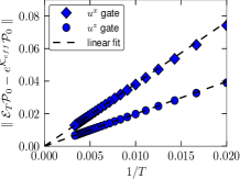
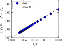
Figure 1: (Color online) Distance of the effective evolution from the exact one as a function of $1/T.$ Left panel: DFS example with $\mathcal{L}_{0}$ given by Eq. (4). We used $\gamma_{\alpha}=1$ and $\vartheta=1$ (see text for details). Right panel: example for noiseless subsystem with parameters $\phi_{j}=\vartheta=1$ (see text). The norm used is the maximum singular value of the maps realized as matrices over ${\cal H}^{\otimes\,2}$. The linear fits are obtained using the four most significant points.

Unitaries over a DFS. :–  We show here how to perform coherent manipulations on a logical qubit built upon the SSM of four qubits which comprises a DFS DFS . Consider the following unperturbed Liouvillian

$$\mathcal{L}_{0}\left(\rho\right)=\sum_{\alpha=x,y,z}\gamma_{\alpha}\left(S^{\alpha}\rho S^{\alpha\dagger}-\frac{1}{2}\left\{S^{\alpha\dagger}S^{\alpha},\rho\right\}\right)$$ (4)

where $S^{\alpha}=\sum_{j=1}^{N}S_{j}^{\alpha}$ are collective spin operators and $\gamma_{\alpha}$ decoherence rates. The interaction algebra $\cal A$ generated by the $S^{\alpha}$’s is the algebra of permutation invariant operators NS . Therefore, from i), it follows that Ker${\cal L}_{0}$ has the structure commutant where $J$ is now a total angular momentum label, $d_{J}=2J+1$ and the $n_{J}$’s are the dimensions of irreps of the permutation group ${\cal S}_{N}$ perm-dim . For $N=4$ the one-dimensional $J=0$ representation shows with multiplicity two. If we denote by ${\cal C}$ this two-dimensional subspace the conditions in ii) are met.

Let us denote with $\Pi$ the projector onto ${\cal C}$. It is known that one can construct universal set of gates in similar DFSs (see e.g. daniel_singlet ) when the dynamics is entirely contained in the DFS. Here we show that coherent manipulation is possible also when the dynamics leaks out of the DFS. Consider for example the following Hamiltonian perturbations $H^{x}=\frac{3}{2}\left(\sigma_{1}^{z}\sigma_{2}^{z}+\sigma_{2}^{z}\sigma_{3}^{z}\right)+\openone$ and $H^{z}=-\frac{\sqrt{3}}{2}\left(\sigma_{1}^{z}\sigma_{2}^{z}-\sigma_{2}^{z}\sigma_{3}^{z}\right)+\sigma_{1}^{z}.$ One can check that in the logical space ${\cal C}$, such Hamiltonians reduce to elementary Pauli operations, i.e. $\Pi H^{\alpha}\Pi=\sigma^{\alpha}$. We now build the perturbed Liouvillians $\mathcal{L}^{\alpha}=\mathcal{L}_{0}-i\vartheta/T\left[H^{\alpha},\bullet\right]$, $\alpha=x,z$, let us also denote $\tilde{\mathcal{K}}_{eff}^{\alpha}=-i\vartheta\mathcal{P}_{0}\left[H^{\alpha},\bullet\right]\mathcal{P}_{0}$ with $\vartheta$ free parameter. In Fig. 1 left panel we show a numerical experiment confirming our general theorem Eq. (3) for such $\mathcal{L}^{\alpha}$. In the logical qubit space, the effective evolution $e^{\tilde{{\cal K}}_{eff}^{\alpha}}$ is a unitary evolution $e^{\tilde{{\cal K}}_{eff}^{\alpha}}(X)\simeq u^{\alpha}Xu^{\alpha\dagger}$ with $u^{\alpha}=\exp(-i\vartheta\sigma^{\alpha})$, and one can easily generate any unitary in $SU(2)$ by concatenating such gates. Moreover, the bound in Eq. (3) implies that, for any vectors $|i\rangle,\,|j\rangle$ in the logical space ${\cal C}$, $\parallel(\mathcal{E}_{T}-e^{\tilde{\mathcal{K}}_{eff}})(|i\rangle\langle j|)\parallel\,\leq\,\parallel(\mathcal{E}_{T}-e^{\tilde{\mathcal{K}}_{eff}})\mathcal{P}_{0}\parallel=O(1/T)$, showing that effectively, one can generate unitary gates on the logical qubit space ${\cal C}$ up to an error $1/T.$ In view of Remark 3) one is allowed to add to $\mathcal{L}^{\alpha}$ any perturbation $\mathcal{V}$ satisfying $\mathcal{P}_{0}\mathcal{V}\mathcal{P}_{0}=0$, and still obtain the same unitary gates $u^{\alpha}$ within an error $c/T$ albeit with a possibly different $c$ inpreparation . In SM we show the stability of this dynamics also against certain dissipative perturbations of ${\cal L}_{0}.$ Fig. 1 (left panel) shows that the whole $14$-dimensional SSM is evolving unitarily in the long time limit.

To illustrate our results let us consider the experimental DFS system studied in DFS-exp consisting of a couple of trapped ${}^{9}Be^{+}$ ions subject to collective dephasing [$\gamma_{x,y}=0$ in (4)]. In this case $\tau_{R}\sim 5\,\mu s$ and (assuming a similar relaxation time for a four qubits system) Eq. (2) and Fig. 1 show that for $T\sim 500\,\mu s$ one should observe small deviations of the effective dynamics from unitarity.

Unitaries over noiseless subsystem:–  Next we discuss dissipation-assisted computation over noiseless subsystems NS . The Liouvillian is in the class previously discussed, $\mathcal{L}_{0}\left(\rho\right)=\Phi\left(\rho\right)-\rho$, taking $\Phi\left(\rho\right)=\frac{1}{3}\sum_{\alpha=1}^{3}U_{\alpha}\rho U_{\alpha}^{\dagger},\quad U_{\alpha}=e^{i\phi_{\alpha}S^{\alpha}},$ where $S^{\alpha}$ are again collective spin operators. For generic $\phi_{\alpha}$’s the SSM coincides with one of the former examples i.e, rotationally invariant state. The latter for an odd number $N$ of spins, contains only mixed states. As perturbation we use the following Hamiltonian $H=\sigma_{1}^{x}\sigma_{2}^{x}$ and the full Liouvillian reads $\mathcal{L}=\mathcal{L}_{0}-i\vartheta/T\left[H,\bullet\right]$. Again one observes an effective unitary evolution, up to an error $O(1/T),$ (see Fig. 1 right panel) over the full five-dimensional SSM; in particular, this construction can be seen as a scheme to enact dissipation-assisted control over the noiseless-subsystem ${\mathbf{C}}^{2}$ factor ogy .

In NS-exp noiseless-subsystems have been realized in a NMR system comprising three nuclear spins subject to collective (artificial) noise; for a relaxation time $\tau_{R}<1/30\,s$ the noiseless encoding provides an advantage. Fig 1 shows that setting the operation time, say at $T=100\,\tau_{R},$ then effective dynamics over the NSs becomes very close to a unitary one.

Finally we would like to stress that the Markovian form (1) is just sufficient (and mathematically convenient) to prove the existence of an effective projected dynamics, not necessary. The spin-boson Hamiltonian discussed in SM indicates that the relevant dynamical mechanism is the existence of a strong system-bath coupling that adiabatically-decouples non steady-states from the dynamics.

Conclusions:–  In this Letter we have shown how an effective unitary dynamics can be enacted over the manifold of steady states of a strongly-dissipative system. The strategy is to introduce a small time-rescaled Hamiltonian term in the system’s Liouvillian largely dominated by the dissipative processes. In the long time limit the dynamics leaves the steady state manifold invariant and becomes unitary up to a small error whose strength is connected to the Liouvillian relaxation time, and total operation time. The effective Hamiltonian ruling the long time-dynamics is shaped by the continuous interplay of the weak Hamiltonian control with the the fast relaxation process that adiabatically decouples non-steady states. This effective projected Hamiltonian, in some cases, can be seen as a symmetrized form of the bare one and it is robust against all perturbations, dissipative or Hamiltonian, that are filtered out by this environment-induced symmetrization.

To illustrate these ideas we have shown how to realize quantum gates on steady-state manifolds comprising decoherence-free subspaces DFS as well as noiseless subsystems NS . In all these cases we have also provided a numerical estimate of the deviations from the ideal long-time unitary behavior and the actual, finite time, one. Agreement with the theoretical prediction (3) is found in all cases.

The results of this Letter seem to suggest the intriguing possibility of fighting quantum decoherence by introducing even more quantum decoherence.

Appendix A Proof of Main Theorem

In this section we provide a proof of Eq. (2) of the main text. Our approach and terminology rely heavily on the classical text kato . Let ${\cal L}_{T}={\cal L}_{0}+T^{-1}\tilde{{\cal K}}$. For $T^{-1}=0$, ${\cal L}_{0}$ is assumed to have a degenerate steady state manifold, i.e. $\dim\ker\mathcal{L}_{0}=m_{0}>1.$ For small non-zero $T^{-1}$, some eigenvalues of $\mathcal{L}_{T}$ (may) depart from $\lambda=0$. The set of these eigenvalues is called the $\lambda$-group since they cluster around the unperturbed eigenvalue, in this case $\lambda=0$, for small $\left|T^{-1}\right|$ kato . Let ${\cal P}$ be the projection associated to the $\lambda$-group originating from the degenerate $\lambda=0$ eigenvalue of ${\cal L}_{0}$ (whose associate projection is given by ${\cal P}_{0}$). Define also the projected Liouvillian ${\cal L}_{r}:={\cal P}{\cal L}_{T}{\cal P}$. A central result of kato states that both $\mathcal{P}$ and $\mathcal{L}_{r}$ are analytic in $T^{-1}$, i.e. their power series in $T^{-1}$ have a finite radius of convergence. Since $\mathcal{P}$ commutes with $\mathcal{L}_{T}$ one clearly has $e^{t{\cal L}_{T}}{\cal P}=e^{t{\cal L}_{r}}{\cal P}$. We can now expand both $\mathcal{P}$ and $\mathcal{L}_{r}$ around $T^{-1}=0$. Accordingly we write

$$e^{t{\cal L}_{T}}({\cal P}_{0}+\delta{\cal P})=e^{t\,{\cal L}_{\mathrm{eff}}+t\,\delta{\cal L}}({\cal P}_{0}+\delta{\cal P}),$$ (5)

where we defined $\delta{\cal P}:={\cal P}-{\cal P}_{0},\,{\cal L}_{\mathrm{eff}}:={\cal P}_{0}{\cal L}_{T}{\cal P}_{0}=T^{-1}{\cal P}_{0}\tilde{{\cal K}}{\cal P}_{0},$ and $\delta{\cal L}:={\cal L}_{r}-{\cal L}_{\mathrm{eff}}.$ Using kato and remembering that $t\leq T$, one finds

$$\|\delta{\cal P}\|=O(1/T),\;\;\|t\,\delta{\cal L}\|=O(1/T),\;\;\|t\,{\cal L}_{\mathrm{eff}}\|=O(1).$$ (6)

For example, in case the zero eigenvalue has no nilpotent part, as it happens in physical systems, one has kato

$${\cal L}_{r} ={\cal P}_{0}{\cal L}_{T}{\cal P}_{0}$$

$$-T^{-2}\Big{(}{\cal P}_{0}\tilde{{\cal K}}{\cal P}_{0}\tilde{{\cal K}}{\cal S}+{\cal P}_{0}\tilde{{\cal K}}{\cal S}\tilde{{\cal K}}{\cal P}_{0}$$

$$+{\cal S}\tilde{{\cal K}}{\cal P}_{0}\tilde{{\cal K}}{\cal P}_{0}\Big{)}+O(T^{-3})$$ (7)

and

$$\delta\mathcal{P}=-T^{-1}\left({\cal P}_{0}\tilde{{\cal K}}{\cal S}+{\cal S}\tilde{{\cal K}}{\cal P}_{0}\right)+O(T^{-2}).$$ (8)

In Eqns. (7) and (8) above, ${\cal S}$ is the projected resolvent of $\mathcal{L}_{0}$ related to the $\lambda=0$ eigenvalue. Explicitly, if $\mathcal{L}_{0}$ has the following Jordan decomposition

$$\mathcal{L}_{0}=\sum_{j=0}^{s-1}\lambda_{j}\mathcal{P}_{j}+\mathcal{D}_{j},$$ (9)

with $\mathcal{P}_{j}$ projectors, $\mathcal{D}_{j}$ nilpotents and $\lambda_{0}=0$, the projected resolvent is given by

$$\mathcal{S}=-\sum_{j=1}^{s-1}\left[(-\lambda_{j})^{-1}\mathcal{P}_{j}+\sum_{n=1}^{m_{j}-1}(-\lambda_{j})^{-n-1}\mathcal{D}_{j}^{n}\right].$$

Define further $\Delta:=e^{t\,{\cal L}_{\mathrm{eff}}+t\,\delta{\cal L}}-e^{t\,{\cal L}_{\mathrm{eff}}}$. Now we use the inequality $\|e^{X+Y}-e^{X}\|\leq\|Y\|e^{\|X\|+\|Y\|}$ with $X=t\,{\cal L}_{\mathrm{eff}}$ and $Y=t\,\delta{\cal L},$ to obtain

$$\|\Delta\|\leq\|t\,\delta{\cal L}\|e^{\|t\,{\cal L}_{\mathrm{eff}}\|+\|t\,\delta{\cal L}\|}.$$ (10)

Therefore

$$e^{t\,{\cal L}}{\cal P}_{0} = e^{t\,{\cal L}_{\mathrm{eff}}}{\cal P}_{0}+{\cal E},$$ (11)

$$\mathrm{with}\quad\mathcal{E} = \Delta(\mathcal{P}_{0}+\delta{\cal P})+(e^{t\,{\cal L}_{\mathrm{eff}}}-e^{t\,{\cal L}})\delta{\cal P}.$$ (12)

The proof is completed using triangle inequality and the bounds (6) and (10) (and setting $t=T$), implying $\|{\cal E}\|=O(1/T)$.

Note that this proof, together with the bound (2) in the main text, remains valid in a slightly more general setting where the eigenvalues $\lambda_{h}$ of $\mathcal{L}$ satisfy $\mathrm{Re}(\lambda_{h})\leq 0$. For example, in the extreme case of unitary dynamics where the eigenvalues are purely imaginary this result become essentially the standard adiabatic theorem as discussed in Sec. B, but intermediate cases are accounted for as well.

We now consider a case in which ${\cal P}_{0}\tilde{{\cal K}}{\cal P}_{0}=0$. Performing the rescaling $\mathcal{K}=T^{1/2}\tilde{\mathcal{K}}$ one is led to analyze $\mathcal{L}_{r}={\cal L}_{\mathrm{eff}}+\delta\mathcal{L}$ with ${\cal L}_{\mathrm{eff}}=-T^{-1}{\cal P}_{0}\tilde{{\cal K}}{\cal S}\tilde{{\cal K}}{\cal P}_{0}$. The bounds in Eq. (6) become now

$$\|\delta{\cal P}\|=O(1/T^{1/2}),\;\;\|t\,\delta{\cal L}\|=O(1/T^{1/2}),\;\;\|t\,{\cal L}_{\mathrm{eff}}\|=O(1).$$ (13)

Reasoning as previously we now obtain $e^{T\,{\cal L}}{\cal P}_{0}=e^{T\,{\cal{\cal L}_{\mathrm{eff}}}}{\cal P}_{0}+{\cal E}$ with $\|{\cal E}\|=O\left(T^{-1/2}\right)$.

Appendix B Hamiltonian example

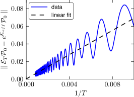
Figure 2: Distance of the effective unitary evolution from the exact (unitary) one one as a function of $1/T$. The norm used is the maximum singular value of the maps realized as matrices over ${\cal H}^{\otimes\,2}.$ Parameter used are $\omega_{k}=k$ ($k=2\pi n/N_{B}$, $n=1,\ldots,N_{B}$), $g_{k}=0.045$ and $\vartheta=1$. The system has $N_{S}=3$ and $N_{B}=60$.

as reminded in the previous section, our projection result Eq. (2) of the main text, holds also when $\mathcal{L}_{0}=-i\left[H_{0},\bullet\right]$ and in this case it simply amounts to a type of adiabatic theorem for closed quantum systems. To illustrate this fact we consider a system of $N_{S}$ spins interacting collectively with $N_{B}$ bosons and Hamiltonian of atoms with the radiation field. We restrict ourself to the space of only one boson or spin excitation Hilbert space $\mathcal{H}=\mathrm{span}\left\{|x\rangle_{S}|0\rangle_{B},|\Downarrow\rangle_{S}|k\rangle_{B}\right\}$, $x=1,\ldots,N_{s},$ $k=1,\ldots,N_{b}$ where $|x\rangle_{S}|0\rangle_{B}=S_{x}^{+}|\Downarrow\rangle_{S}|k\rangle_{B}$, $|\Downarrow\rangle_{S}$ has all spins down, $|k\rangle_{B}$ one boson in mode $k$ and $|0\rangle_{B}$ is the boson vacuum. Hamiltonian $H_{0}$ admits the following dark states ($H_{0}|\psi_{q}\rangle=0$), $|\psi_{q}\rangle=N_{S}^{-1/2}\sum_{x=1}^{N_{S}}e^{-i2\pi qx/N_{s}}|x\rangle_{S}|0\rangle_{B}$, with $q=1,\ldots,N_{s}-1$ zan97 . SSM includes all the states built over the dark state manifold all of which are decoherence-free at zero temperature zan97 . Let us now introduce an Hamiltonian perturbation which conserves the total number of excitations, such as $H_{1}=\sigma_{1}^{z}$, and the corresponding superoperator $\mathcal{K}=-i\vartheta/T\left[H_{1},\bullet\right]$. projected Hamiltonian over the dark-state manifold turns out to be $\tilde{K}_{eff}=\vartheta[2(N_{S}-1)/N_{s}|\phi\rangle\langle\phi|-\openone]$ with $|\phi\rangle=(N_{S}-1)^{-1/2}\sum_{k=1}^{N_{s}-1}e^{-i2\pi k/N_{S}}|\psi_{k}\rangle$, shows how Eq. (2) of the main text is fulfilled in this unitary case as well.

References

- (1) T. Kato, Perturbation Theory for Linear Operators , Springer 1995
- (2) P. Zanardi, Phys. Rev. A 56, 4445 (1997)