Subspace Learning and Imputation for
Streaming Big Data Matrices and Tensors^†

Abstract

Extracting latent low-dimensional structure from high-dimensional data is of paramount importance in timely inference tasks encountered with ‘Big Data’ analytics. However, increasingly noisy, heterogeneous, and incomplete datasets as well as the need for real-time processing of streaming data pose major challenges to this end. In this context, the present paper permeates benefits from rank minimization to scalable imputation of missing data, via tracking low-dimensional subspaces and unraveling latent (possibly multi-way) structure from incomplete streaming data. For low-rank matrix data, a subspace estimator is proposed based on an exponentially-weighted least-squares criterion regularized with the nuclear norm. After recasting the non-separable nuclear norm into a form amenable to online optimization, real-time algorithms with complementary strengths are developed and their convergence is established under simplifying technical assumptions. In a stationary setting, the asymptotic estimates obtained offer the well-documented performance guarantees of the batch nuclear-norm regularized estimator. Under the same unifying framework, a novel online (adaptive) algorithm is developed to obtain multi-way decompositions of low-rank tensors with missing entries, and perform imputation as a byproduct. Simulated tests with both synthetic as well as real Internet and cardiac magnetic resonance imagery (MRI) data confirm the efficacy of the proposed algorithms, and their superior performance relative to state-of-the-art alternatives.

Submitted:

I Introduction

Nowadays ubiquitous e-commerce sites, the Web, and Internet-friendly portable devices generate massive volumes of data. The overwhelming consensus is that tremendous economic growth and improvement in quality of life can be effected by harnessing the potential benefits of analyzing this large volume of data. As a result, the problem of extracting the most informative, yet low-dimensional structure from high-dimensional datasets is of paramount importance [22]. The sheer volume of data and the fact that oftentimes observations are acquired sequentially in time, motivate updating previously obtained ‘analytics’ rather than re-computing new ones from scratch each time a new datum becomes available [37, 29]. In addition, due to the disparate origins of the data, subsampling for faster data acquisition, or even privacy constraints, the datasets are often incomplete [13, 3].

In this context, consider streaming data comprising incomplete and noisy observations of the signal of interest ${\bf x}_{t}\in\mathbb{R}^{P}$ at time $t=1,2,\ldots$. Depending on the application, these acquired vectors could e.g., correspond to (vectorized) images, link traffic measurements collected across physical links of a computer network, or, movie ratings provided by Netflix users. Suppose that the signal sequence $\{{\bf x}_{t}\}_{t=1}^{\infty}$ lives in a low-dimensional ($\ll P$) linear subspace $\mathcal{L}_{t}$ of $\mathbb{R}^{P}$. Given the incomplete observations that are acquired sequentially in time, this paper deals first with (adaptive) online estimation of $\mathcal{L}_{t}$, and reconstruction of the signal ${\bf x}_{t}$ as a byproduct. This problem can be equivalently viewed as low-rank matrix completion with noise [13], solved online over $t$ indexing the columns of relevant matrices, e.g., ${\bf X}_{t}:=[{\bf x}_{1},\ldots,{\bf x}_{t}]$.

Modern datasets are oftentimes indexed by three or more variables giving rise to a tensor, that is a data cube or a mutli-way array, in general [25]. It is not uncommon that one of these variables indexes time [33], and that sizable portions of the data are missing [7, 3, 20, 28, 35]. Various data analytic tasks for network traffic, social networking, or medical data analysis aim at capturing underlying latent structure, which calls for high-order tensor factorizations even in the presence of missing data [7, 3, 28]. It is in principle possible to unfold the given tensor into a matrix and resort to either batch [34, 20], or, online matrix completion algorithms as the ones developed in the first part of this paper; see also [31, 4, 15]. However, tensor models preserve the multi-way nature of the data and extract the underlying factors in each mode (dimension) of a higher-order array. Accordingly, the present paper also contributes towards fulfilling a pressing need in terms of analyzing streaming and incomplete multi-way data; namely, low-complexity, real-time algorithms capable of unraveling latent structures through parsimonious (e.g., low-rank) decompositions, such as the parallel factor analysis (PARAFAC) model; see e.g. [25] for a comprehensive tutorial treatment on tensor decompositions, algorithms, and applications.

Relation to prior work. Subspace tracking has a long history in signal processing. An early noteworthy representative is the projection approximation subspace tracking (PAST) algorithm [42]; see also [43]. Recently, an algorithm (termed GROUSE) for tracking subspaces from incomplete observations was put forth in [4], based on incremental gradient descent iterations on the Grassmannian manifold of subspaces. Recent analysis has shown that GROUSE can converge locally at an expected linear rate [6], and that it is tightly related to the incremental SVD algorithm [5]. PETRELS is a second-order recursive least-squares (RLS)-type algorithm, that extends the seminal PAST iterations to handle missing data [15]. As noted in [16], the performance of GROUSE is limited by the existence of barriers in the search path on the Grassmanian, which may lead to GROUSE iterations being trapped at local minima; see also [15]. Lack of regularization in PETRELS can also lead to unstable (even divergent) behaviors, especially when the amount of missing data is large. Accordingly, the convergence results for PETRELS are confined to the full-data setting where the algorithm boils down to PAST [15]. Relative to all aforementioned works, the algorithmic framework of this paper permeates benefits from rank minimization to low-dimensional subspace tracking and missing data imputation (Section III), offers provable convergence and theoretical performance guarantees in a stationary setting (Section IV), and is flexible to accommodate tensor streaming data models as well (Section V). While algorithms to impute incomplete tensors have been recently proposed in e.g., [20, 7, 3, 28], all existing approaches rely on batch processing.

Contributions. Leveraging the low dimensionality of the underlying subspace $\mathcal{L}_{t}$, an estimator is proposed based on an exponentially-weighted least-squares (EWLS) criterion regularized with the nuclear norm of ${\bf X}_{t}$. For a related data model, similar algorithmic construction ideas were put forth in our precursor paper [31], which dealt with real-time identification of network traffic anomalies. Here instead, the focus is on subspace tracking from incomplete measurements, and online matrix completion. Upon recasting the non-separable nuclear norm into a form amenable to online optimization as in [31], real-time subspace tracking algorithms with complementary strengths are developed in Section III, and their convergence is established under simplifying technical assumptions. For stationary data and under mild assumptions, the proposed online algorithms provably attain the global optimum of the batch nuclear-norm regularized problem (Section IV-C), whose quantifiable performance has well-appreciated merits [13, 12]. This optimality result as well as the convergence of the (first-order) stochastic-gradient subspace tracker established in Section IV-B, markedly broaden and complement the convergence claims in [31].

The present paper develops for the first time an online algorithm for decomposing low-rank tensors with missing entries; see also [33] for an adaptive algorithm to obtain PARAFAC decompositions with full data. Accurately approximating a given incomplete tensor allows one to impute those missing entries as a byproduct, by simply reconstructing the data cube from the model factors (which for PARAFAC are unique under relatively mild assumptions [26, 9]). Leveraging stochastic gradient-descent iterations, a scalable, real-time algorithm is developed in Section V under the same rank-minimization framework utilized for the matrix case, which here entails minimizing an EWLS fitting error criterion regularized by separable Frobenius norms of the PARAFAC decomposition factors [7]. The proposed online algorithms offer a viable approach to solving large-scale tensor decomposition (and completion) problems, even if the data is not actually streamed but they are so massive that do not fit in the main memory.

Simulated tests with synthetic as well as real Internet traffic data corroborate the effectiveness of the proposed algorithms for traffic estimation and anomaly detection, and its superior performance relative to state-of-the-art alternatives (available only for the matrix case [4, 15]). Additional tests with cardiac magnetic resonance imagery (MRI) data confirm the efficacy of the proposed tensor algorithm in imputing up to $75\%$ missing entries. Conclusions are drawn in Section VII.

Notation: Bold uppercase (lowercase) letters will denote matrices (column vectors), and calligraphic letters will be used for sets. Operators $(\cdot)^{\prime}$, $\rm{tr}(\cdot)$, $\mathbbm{E}[\cdot]$, $\sigma_{\max}(\cdot)$, $\odot$, and $\circ$ will denote transposition, matrix trace, statistical expectation, maximum singular value, Hadamard product, and outer product, respectively; $|\cdot|$ will be used for the cardinality of a set, and the magnitude of a scalar. The positive semidefinite matrix $\mathbf{M}$ will be denoted by ${\mathbf{M}}\succeq\mathbf{0}$. The $\ell_{p}$-norm of ${\bf x}\in\mathbb{R}^{n}$ is $\|{\bf x}\|_{p}:=(\sum_{i=1}^{n}|x_{i}|^{p})^{1/p}$ for $p\geq 1$. For two matrices ${\bf M},{\bf U}\in\mathbb{R}^{n\times p}$, $\langle{\bf M},{\bf U}\rangle:=\rm{tr({\bf M}^{\prime}{\bf U})}$ denotes their trace inner product, and $\|{\bf M}\|_{F}:=\sqrt{\text{tr}({\bf M}{\bf M}^{\prime})}$ is the Frobenious norm. The $n\times n$ identity matrix will be represented by ${\bf I}_{n}$, while $\mathbf{0}_{n}$ will stand for the $n\times 1$ vector of all zeros, $\mathbf{0}_{n\times p}:=\mathbf{0}_{n}\mathbf{0}^{\prime}_{p}$, and $[n]:=\{1,2,\ldots,n\}$.

II Preliminaries and Problem Statement

Consider a sequence of high-dimensional data vectors, which are corrupted with additive noise and some of their entries may be missing. At time $t$, the incomplete streaming observations are modeled as

$$\mathcal{P}_{\omega_{t}}({\bf y}_{t})=\mathcal{P}_{\omega_{t}}({\bf x}_{t}+{\bf v}_{t}),\quad t=1,2,\ldots$$ (1)

where ${\bf x}_{t}\in\mathbb{R}^{P}$ is the signal of interest, and ${\bf v}_{t}$ stands for the noise. The set $\omega_{t}\subset\{1,2,\ldots,P\}$ contains the indices of available observations, while the corresponding sampling operator $\mathcal{P}_{\omega_{t}}(\cdot)$ sets the entries of its vector argument not in $\omega_{t}$ to zero, and keeps the rest unchanged; note that $\mathcal{P}_{\omega_{t}}({\bf y}_{t})\in\mathbb{R}^{P}$. Suppose that the sequence $\{{\bf x}_{t}\}_{t=1}^{\infty}$ lives in a low-dimensional ($\ll P$) linear subspace $\mathcal{L}_{t}$, which is allowed to change slowly over time. Given the incomplete observations $\{\mathcal{P}_{\omega_{\tau}}({\bf y}_{\tau})\}_{\tau=1}^{t}$, the first part of this paper deals with online (adaptive) estimation of $\mathcal{L}_{t}$, and reconstruction of ${\bf x}_{t}$ as a byproduct. The reconstruction here involves imputing the missing elements, and denoising the observed ones.

II-A Challenges facing large-scale nuclear norm minimization

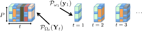
Figure 1: Matrix data with missing entries. (Left) Batch data ${\cal P}_{\Omega_{t}}({\bf Y}_{t})$ available at time $t$. (Right) Streaming data, where vectors ${\cal P}_{\omega_{t}}({\bf y}_{t})$ become available for $t=1,2,\ldots$.

Collect the indices of available observations up to time $t$ in the set $\Omega_{t}:=\cup_{\tau=1}^{t}\omega_{\tau}$, and the actual batch of observations in the matrix $\mathcal{P}_{\Omega_{t}}({\bf Y}_{t}):=[\mathcal{P}_{\omega_{1}}({\bf y}_{1}),\ldots,\mathcal{P}_{\omega_{t}}({\bf y}_{t})]\in\mathbb{R}^{P\times t}$; see also Fig. 1. Likewise, introduce matrix ${\bf X}_{t}$ containing the signal of interest. Since ${\bf x}_{t}$ lies in a low-dimensional subspace, ${\bf X}_{t}$ is (approximately) a low-rank matrix. A natural estimator leveraging the low rank property of ${\bf X}_{t}$ attempts to fit the incomplete data $\mathcal{P}_{\Omega_{t}}({\bf Y}_{t})$ to ${\bf X}_{t}$ in the least-squares (LS) sense, as well as minimize the rank of ${\bf X}_{t}$. Unfortunately, albeit natural the rank criterion is in general NP-hard to optimize [34]. This motivates solving for [13]

$$\text{(P1)}~{}~{}~{}~{}\hat{{\bf X}}_{t}:=\arg\min_{{\bf X}}\left\{\frac{1}{2}\|\mathcal{P}_{\Omega_{t}}({\bf Y}_{t}-{\bf X})\|_{F}^{2}+\lambda_{t}\|{\bf X}\|_{\ast}\right\}$$

where the nuclear norm $\|{\bf X}_{t}\|_{*}:=\sum_{k}\sigma_{k}({\bf X}_{t})$ ($\sigma_{k}$ is the $k$-th singular value) is adopted as a convex surrogate to $\textrm{rank}({\bf X}_{t})$ [17], and $\lambda_{t}$ is a (possibly time-varying) rank-controlling parameter. Scalable imputation algorithms for streaming observations should effectively overcome the following challenges: (c1) the problem size can easily become quite large, since the number of optimization variables $Pt$ grows with time; (c2) existing batch iterative solvers for (P1) typically rely on costly SVD computations per iteration; see e.g., [12]; and (c3) (columnwise) nonseparability of the nuclear-norm challenges online processing when new columns $\{\mathcal{P}_{\omega_{t}}({\bf y}_{t})\}$ arrive sequentially in time. In the following subsection, the ‘Big Data’ challenges (c1)-(c3) are dealt with to arrive at an efficient online algorithm in Section III.

II-B A separable low-rank regularization

To limit the computational complexity and memory storage requirements of the algorithm sought, it is henceforth assumed that the dimensionality of the underlying time-varying subspace $\mathcal{L}_{t}$ is bounded by a known quantity $\rho$. Accordingly, it is natural to require $\textrm{rank}(\hat{{\bf X}}_{t})\leq\rho$. As argued later in Remark 1, the smaller the value of $\rho$, the more efficient the algorithm becomes. Because $\textrm{rank}(\hat{{\bf X}}_{t})\leq\rho$ one can factorize the matrix decision variable as ${\bf X}={\bf L}{\bf Q}^{\prime}$, where ${\bf L}$ and ${\bf Q}$ are $P\times\rho$ and $t\times\rho$ matrices, respectively. Such a bilinear decomposition suggests $\mathcal{L}_{t}$ is spanned by the columns of ${\bf L}$, while the rows of ${\bf Q}$ are the projections of $\{{\bf x}_{t}\}$ onto $\mathcal{L}_{t}$.

To address (c1) and (c2) [along with (c3) as it will become clear in Section III], consider the following alternative characterization of the nuclear norm [40]

$$\|{\bf X}\|_{*}:=\min_{\{{\bf L},{\bf Q}\}}~{}~{}~{}\frac{1}{2}\left\{\|{\bf L}\|_{F}^{2}+\|{\bf Q}\|_{F}^{2}\right\},\quad\text{s. to}~{}~{}~{}{\bf X}={\bf L}{\bf Q}^{\prime}.$$ (2)

The optimization (2) is over all possible bilinear factorizations of ${\bf X}$, so that the number of columns $\rho$ of ${\bf L}$ and $\mathbf{Q}$ is also a variable. Leveraging (2), the following nonconvex reformulation of (P1) provides an important first step towards obtaining an online algorithm:

$$\text{(P2)}~{}~{}~{}~{}~{}\min_{\{{\bf L},{\bf Q}\}} \frac{1}{2}\|\mathcal{P}_{\Omega_{t}}({\bf Y}_{t}-{\bf L}{\bf Q}^{\prime})\|_{F}^{2}+\frac{\lambda_{t}}{2}\left\{\|{\bf L}\|_{F}^{2}+\|{\bf Q}\|_{F}^{2}\right\}.$$

The number of variables is reduced from $Pt$ in (P1) to $\rho(P+t)$ in (P2), which can be significant when $\rho$ is small, and both $P$ and $t$ are large. Most importantly, it follows that adopting the separable (across the time-indexed columns of ${\bf Q}$) Frobenius-norm regularization in (P2) comes with no loss of optimality relative to (P1), provided $\rho\geq\textrm{rank}({\hat{\bf X}}_{t})$.

By finding the global minimum of (P2), one can recover the optimal solution of (P1). However, since (P2) is nonconvex, it may have stationary points which need not be globally optimum. Interestingly, results in [30, 11] offer a global optimality certificate for stationary points of (P2). Specifically, if $\{\bar{{\bf L}}_{t},\bar{{\bf Q}}_{t}\}$ is a stationary point of (P2) (obtained with any practical solver) satisfying the qualification inequality $\sigma_{\max}[\mathcal{P}_{\Omega_{t}}({\bf Y}_{t}-\bar{{\bf L}}_{t}\bar{{\bf Q}}^{\prime}_{t})]\leq\lambda_{t}$, then ${\hat{{\bf X}}}_{t}:=\bar{{\bf L}}_{t}\bar{{\bf Q}}^{\prime}_{t}$ is the globally optimal solution of (P1) [30, 11].

III Online Rank Minization for Matrix Imputation

In ‘Big Data’ applications the collection of massive amounts of data far outweigh the ability of modern computers to store and analyze them as a batch. In addition, in practice (possibly incomplete) observations are acquired sequentially in time which motivates updating previously obtained estimates rather than re-computing new ones from scratch each time a new datum becomes available. As stated in Section II, the goal is to recursively track the low-dimensional subspace $\mathcal{L}_{t}$, and subsequently estimate $\hat{{\bf x}}_{t}$ per time $t$ from historical observations $\{\mathcal{P}_{\omega_{\tau}}({\bf y}_{\tau})\}_{\tau=1}^{t}$, naturally placing more importance on recent measurements. To this end, one possible adaptive counterpart to (P2) is the exponentially-weighted LS (EWLS) estimator found by minimizing the empirical cost

$${\rm(P3)}~{}~{}~{}\min_{\{{\bf L},{\bf Q}\}}\sum_{\tau=1}^{t}\theta^{t-\tau}\left[\frac{1}{2}\|\mathcal{P}_{\omega_{\tau}}({\bf y}_{\tau}-{\bf L}{\bf q}_{\tau})\|_{2}^{2}+\frac{\bar{\lambda}_{t}}{2}\|{\bf L}\|_{F}^{2}+\frac{\lambda_{t}}{2}\|{\bf q}_{\tau}\|_{2}^{2}\right]$$

where ${\bf Q}:=[{\bf q}_{1},\ldots,{\bf q}_{t}]$, $\bar{\lambda}_{t}:=\lambda_{t}/\sum_{\tau=1}^{t}\theta^{t-\tau}$, and $0<\theta\leq 1$ is the so-termed forgetting factor. When $\theta<1$, data in the distant past are exponentially downweighted, which facilitates tracking in nonstationary environments. In the case of infinite memory $(\theta=1)$, the formulation (P3) coincides with the batch estimator (P2). This is the reason for the time-varying factor $\bar{\lambda}_{t}$ weighting $\|{\bf L}\|_{F}^{2}$.

We first introduced the basic idea of performing online rank-minimization leveraging the separable nuclear-norm regularization (2) in [31] (and its conference precursor), in the context of unveiling network traffic anomalies. Since then, the approach has gained popularity in real-time non-negative matrix factorization for singing voice separation from its music accompaniment [39], and online robust PCA [18], too name a few examples. Instead, the novelty here is on subspace tracking from incomplete measurements, as well as online low-rank matrix and tensor completion.

III-A Alternating recursive LS for subspace tracking from incomplete data

Towards deriving a real-time, computationally efficient, and recursive solver of (P3), an alternating-minimization (AM) method is adopted in which iterations coincide with the time-scale $t$ of data acquisition. A justification in terms of minimizing a suitable approximate cost function is discussed in detail in Section IV-A. Per time instant $t$, a new datum $\{\mathcal{P}_{\omega_{t}}({\bf y}_{t})\}$ is drawn and ${\bf q}_{t}$ is estimated via

$${\bf q}[t]=\arg\min_{{\bf q}}\left[\frac{1}{2}\|\mathcal{P}_{\omega_{t}}({\bf y}_{t}-{\bf L}[t-1]{\bf q})\|_{2}^{2}+\frac{\lambda_{t}}{2}\|{\bf q}\|_{2}^{2}\right]$$ (3)

which is an $\ell_{2}$-norm regularized LS (ridge-regression) problem. It admits the closed-form solution

$${\bf q}[t] =\left(\lambda_{t}{\bf I}_{\rho}+{\bf L}^{\prime}[t-1]\mathbf{\Omega}_{t}{\bf L}[t-1]\right)^{-1}{\bf L}^{\prime}[t-1]\mathcal{P}_{\omega_{t}}({\bf y}_{t})$$ (4)

where diagonal matrix $\mathbf{\Omega}_{t}\in\{0,1\}^{P\times P}$ is such that $[\mathbf{\Omega}_{t}]_{p,p}=1$ if $p\in\omega_{t}$, and is zero elsewhere. In the second step of the AM scheme, the updated subspace matrix ${\bf L}[t]$ is obtained by minimizing (P3) with respect to ${\bf L}$, while the optimization variables $\{{\bf q}_{\tau}\}_{\tau=1}^{t}$ are fixed and take the values $\{{\bf q}[\tau]\}_{\tau=1}^{t}$, namely

$${\bf L}[t]=\arg\min_{{\bf L}}\left[\frac{\lambda_{t}}{2}\|{\bf L}\|_{F}^{2}+\sum_{\tau=1}^{t}\theta^{t-\tau}\frac{1}{2}\|\mathcal{P}_{\omega_{\tau}}({\bf y}_{\tau}-{\bf L}{\bf q}[\tau])\|_{2}^{2}\right].$$ (5)

Notice that (5) decouples over the rows of ${\bf L}$ which are obtained in parallel via

$${\bf l}_{p}[t]= \arg\min_{{\bf l}}\left[\frac{\lambda_{t}}{2}\|{\bf l}\|_{2}^{2}+\sum_{\tau=1}^{t}\theta^{t-\tau}\omega_{p,\tau}(y_{p,\tau}-{\bf l}^{\prime}{\bf q}[\tau])^{2}\right],$$ (6)

for $p=1,\ldots,P$, where $\omega_{p,\tau}$ denotes the $p$-th diagonal entry of $\bm{\Omega}_{\tau}$. For $\theta=1$ and fixed $\lambda_{t}=\lambda,~{}\forall t$, subproblems (6) can be efficiently solved using recursive LS (RLS) [38]. Upon defining ${\bf s}_{p}[t]:=\sum_{\tau=1}^{t}\theta^{t-\tau}\omega_{p,\tau}y_{p,\tau}{\bf q}[\tau]$, ${\bf H}_{p}[t]:=\sum_{\tau=1}^{t}\theta^{t-\tau}\omega_{p,\tau}{\bf q}[\tau]{\bf q}^{\prime}[\tau]+\lambda_{t}{\bf I}_{\rho}$, and ${\bf M}_{p}[t]:={\bf H}_{p}^{-1}[t]$, one updates

$${\bf s}_{p}[t]{}={} {\bf s}_{p}[t-1]+\omega_{p,t}y_{p,t}{\bf q}[t]$$

$${\bf M}_{p}[t]{}={} {\bf M}_{p}[t-1]-\omega_{p,t}\frac{{\bf M}_{p}[t-1]{\bf q}[t]{\bf q}^{\prime}[t]{\bf M}_{p}[t-1]}{1+{\bf q}^{\prime}[t]{\bf M}_{p}[t-1]{\bf q}[t]}$$

and forms ${\bf l}_{p}[t]={\bf M}_{p}[t]{\bf s}_{p}[t]$, for $p=1,\ldots,P$.

However, for $0<\theta<1$ the regularization term $(\lambda_{t}/2)\|{\bf l}\|_{2}^{2}$ in (6) makes it impossible to express ${\bf H}_{p}[t]$ in terms of ${\bf H}_{p}[t-1]$ plus a rank-one correction. Hence, one cannot resort to the matrix inversion lemma and update ${\bf M}_{p}[t]$ with quadratic complexity only. Based on direct inversion of each ${\bf H}_{p}[t]$, the alternating recursive LS algorithm for subspace tracking from incomplete data is tabulated under Algorithm 1.

Algorithm 1 : Alternating LS for subspace tracking from incomplete observations

  input $\{\mathcal{P}_{\omega_{\tau}}({\bf y}_{\tau}),\omega_{\tau}\}_{{\tau}=1}^{\infty}$, $\{\lambda_{\tau}\}_{\tau=1}^{\infty}$, and $\theta$.

  initialize ${\bf G}_{p}[0]=\mathbf{0}_{\rho\times\rho}$, ${\bf s}_{p}[0]=\mathbf{0}_{\rho},~{}p=1,...,P$, and ${\bf L}[0]$ at random.

  for $t=1,2$,$\ldots$ do

     ${\bf D}[t]=\left(\lambda_{t}{\bf I}_{\rho}+{\bf L}^{\prime}[t-1]\mathbf{\Omega}_{t}{\bf L}[t-1]\right)^{-1}{\bf L}^{\prime}[t-1]$.

     ${\bf q}[t]={\bf D}[t]\mathcal{P}_{\omega_{t}}({\bf y}_{t})$.

     ${\bf G}_{p}[t]=\theta{\bf G}_{p}[t-1]+\omega_{p,t}{\bf q}[t]{\bf q}[t]^{\prime},\quad p=1,\ldots,P$.

     ${\bf s}_{p}[t]=\theta{\bf s}_{p}[t-1]+\omega_{p,t}y_{p,t}{\bf q}[t],\quad p=1,\ldots,P$.

     ${\bf l}_{p}[t]=\left({\bf G}_{p}[t]+\lambda_{t}{\bf I}_{\rho}\right)^{-1}{\bf s}_{p}[t],\quad p=1,...,P$.

     return  $\hat{{\bf x}}_{t}:={\bf L}[t]{\bf q}[t]$.

  end for

Remark 1 (Computational cost)

Careful inspection of Algorithm 1 reveals that the main computational burden stems from $\rho\times\rho$ inversions to update the subspace matrix ${\bf L}[t]$. The per iteration complexity for performing the inversions is $\mathcal{O}(P\rho^{3})$ (which could be further reduced if one leverages also the symmetry of ${\bf G}_{p}[t]$), while the cost for the rest of operations including multiplication and additions is $\mathcal{O}(P\rho^{2})$. The overall cost of the algorithm per iteration can thus be safely estimated as $\mathcal{O}(P\rho^{3})$, which can be affordable since $\rho$ is typically small (cf. the low rank assumption). In addition, for the infinite memory case $\theta=1$ where the RLS update is employed, the overall cost is further reduced to $\mathcal{O}(|\omega_{t}|\rho^{2})$.

Remark 2 (Tuning ${\lambda_{t}}$)

To tune $\lambda_{t}$ one can resort to the heuristic rules proposed in [13], which apply under the following assumptions: i) $v_{p,t}\sim\mathcal{N}(0,\sigma^{2})$; ii) elements of $\Omega_{t}$ are independently sampled with probability $\pi$; and, iii) $P$ and $t$ are large enough. Accordingly, one can pick $\lambda_{t}=\big{(}\sqrt{P}+\sqrt{t_{e}}\big{)}\sqrt{\pi}\sigma$, where $t_{e}:=\sum_{\tau=1}^{t}\theta^{t-\tau}$ is the effective time window. Note that $\lambda_{t}$ naturally increases with time when $\theta=1$, whereas for $\theta<1$ a fixed value $\lambda_{t}=\lambda$ is well justified since the data window is effectively finite.

III-B Low-complexity stochastic-gradient subspace updates

Towards reducing Algorithm’s 1 computational complexity in updating the subspace ${\bf L}[t]$, this section aims at developing lightweight algorithms which better suit the ‘Big Data’ landscape. To this end, the basic AM framework in Section III-A will be retained, and the update for ${\bf q}[t]$ will be identical [cf. (4)]. However, instead of exactly solving an unconstrained quadratic program per iteration to obtain ${\bf L}[t]$ [cf. (5)], the subspace estimates will be obtained via stochastic-gradient descent (SGD) iterations. As will be shown later on, these updates can be traced to inexact solutions of a certain quadratic program different from (5).

For $\theta=1$, it is shown in Section IV-A that Algorithm 1’s subspace estimate ${\bf L}[t]$ is obtained by minimizing the empirical cost function $\hat{C}_{t}({\bf L})=(1/t)\sum_{\tau=1}^{t}f_{\tau}({\bf L})$, where

$$f_{t}({\bf L}):=\frac{1}{2}\|\mathcal{P}_{{\omega}_{t}}({\mathbf{y}}_{t}-{\bf L}{\mathbf{q}}[t])\|_{2}^{2}+\frac{\lambda}{2t}\|{\bf L}\|_{F}^{2}+\frac{\lambda}{2}\|{\bf q}[t]\|_{2}^{2},\quad t=1,2,\ldots$$ (7)

By the law of large numbers, if data $\{\mathcal{P}_{\omega_{t}}({\bf y}_{t})\}_{t=1}^{\infty}$ are stationary, solving $\min_{{\bf L}}\lim_{t\to\infty}\hat{C}_{t}({\bf L})$ yields the desired minimizer of the expected cost $\mathbb{E}[C_{t}({\bf L})]$, where the expectation is taken with respect to the unknown probability distribution of the data. A standard approach to achieve this same goal – typically with reduced computational complexity – is to drop the expectation (or the sample averaging operator for that matter), and update the subspace via SGD; see e.g., [38]

$${\bf L}[t]{}={\bf L}[t-1]-(\mu[t])^{-1}\nabla f_{t}({\bf L}[t-1])$$ (8)

where $(\mu[t])^{-1}$ is the step size, and $\nabla f_{t}({\bf L})=-\mathcal{P}_{{\omega}_{t}}({\mathbf{y}}_{t}-{\bf L}{\mathbf{q}}[t]){\mathbf{q}}^{\prime}[t]+(\lambda/t){\bf L}$. The subspace update ${\bf L}[t]$ is nothing but the minimizer of a second-order approximation $Q_{\mu[t],t}({\bf L},{\bf L}[t-1])$ of $f_{t}({\bf L})$ around the previous subspace ${\bf L}[t-1]$, where

$$Q_{\mu,t}({\bf L}_{1},{\bf L}_{2}):=f_{t}({\bf L}_{2})+\langle{\bf L}_{1}-{\bf L}_{2},\nabla f_{t}({\bf L}_{2})\rangle+\frac{\mu}{2}\|{\bf L}_{1}-{\bf L}_{2}\|_{f}^{2}.$$ (9)

To tune the step size, the backtracking rule is adopted, whereby the non-increasing step size sequence $\{(\mu[t])^{-1}\}$ decreases geometrically at certain iterations to guarantee the quadratic function $Q_{\mu[t],t}({\bf L},{\bf L}[t-1])$ majorizes $f_{t}({\bf L})$ at the new update ${\bf L}[t]$. Other choices of the step size are discussed in Section IV. It is observed that different from Algorithm 1, no matrix inversions are involved in the update of the subspace ${\bf L}[t]$. In the context of adaptive filtering, first-order SGD algorithms such as (7) are known to converge slower than RLS. This is expected since RLS can be shown to be an instance of Newton’s (second-order) optimization method [38, Ch. 4].

Algorithm 2 : Online SGD for subspace tracking from incomplete observations

  input $\{\mathcal{P}_{\omega_{\tau}}({\bf y}_{\tau}),\omega_{\tau}\}_{\tau=1}^{\infty},$ $\rho,\lambda,\eta>1$.

  initialize ${\bf L}[0]$ at random, $\mu[0]>0$, $\tilde{\bf L}[1]:={\bf L}[0]$, and $k[1]:=1$.

  for $t=1,2$,$\ldots$ do

     ${\bf D}[t]=\left(\lambda{\bf I}_{\rho}+{\bf L}^{\prime}[t-1]\mathbf{\Omega}_{t}{\bf L}[t-1]\right)^{-1}{\bf L}^{\prime}[t-1]$

     ${\bf q}[t]={\bf D}[t]\mathcal{P}_{\omega_{t}}({\bf y}_{t})$

     Find the smallest nonnegative integer $i[t]$ such that with $\bar{\mu}:=\eta^{i[t]}\mu[t-1]$

$$f_{t}(\tilde{\bf L}[t]-(1/\bar{\mu})\nabla f_{t}(\tilde{\bf L}[t]))\leq Q_{\bar{\mu},t}(\tilde{\bf L}[t]-(1/\bar{\mu})\nabla f_{t}(\tilde{\bf L}[t]),\tilde{\bf L}[t])$$

holds, and set $\mu[t]=\eta^{i[t]}\mu[t-1].$

     ${\bf L}[t]=\tilde{\bf L}[t]-(1/\mu[t])\nabla f_{t}(\tilde{\bf L}[t]).$

     $k[t+1]=\frac{1+\sqrt{1+4k^{2}[t]}}{2}.$

     $\tilde{\bf L}[t+1]={\bf L}[t]+\left(\frac{k[t]-1}{k[t+1]}\right)({\bf L}[t]-{\bf L}[t-1]).$

  end for

  return  $\hat{{\mathbf{x}}}[t]:={\bf L}[t]{\mathbf{q}}[t]$.

Building on the increasingly popular accelerated gradient methods for batch smooth optimization [32, 8], the idea here is to speed-up the learning rate of the estimated subspace (8), without paying a penalty in terms of computational complexity per iteration. The critical difference between standard gradient algorithms and the so-termed Nesterov’s variant, is that the accelerated updates take the form ${\bf L}[t]=\tilde{\bf L}[t]-(\mu[t])^{-1}\nabla f_{t}(\tilde{\bf L}[t])$, which relies on a judicious linear combination $\tilde{\bf L}[t-1]$ of the previous pair of iterates $\{{\bf L}[t-1],{\bf L}[t-2]\}$. Specifically, the choice $\tilde{\bf L}[t]={\bf L}[t-1]+\frac{k[t-1]-1}{k[t]}\left({\bf L}[t-1]-{\bf L}[t-2]\right)$, where $k[t]=\left[1+\sqrt{4k^{2}[t-1]+1}\right]/2$, has been shown to significantly accelerate batch gradient algorithms resulting in convergence rate no worse than $\mathcal{O}(1/k^{2})$; see e.g., [8] and references therein. Using this acceleration technique in conjunction with a backtracking stepsize rule [10], a fast online SGD algorithm for imputing missing entries is tabulated under Algorithm 2. Clearly, a standard (non accelerated) SGD algorithm with backtracking step size rule is subsumed as a special case, when $k[t]=1$, $t=1,2,\ldots$. In this case, complexity is $\mathcal{O}(|\omega_{t}|\rho^{2})$ mainly due to update of ${\bf q}_{t}$, while the accelerated algorithm incurs an additional cost $O(P\rho)$ for the subspace extrapolation step.

IV Performance Guarantees

This section studies the performance of the proposed first- and second-order online algorithms for the infinite memory special case; that is $\theta=1$. In the sequel, to make the analysis tractable the following assumptions are adopted:

(A1) Processes $\{\omega_{t}\}_{t=1}^{\infty}$ and $\{\mathcal{P}_{\omega_{t}}({\bf y}_{t})\}_{t=1}^{\infty}$ are independent and identically distributed (i.i.d.);

(A2) Sequence $\{\mathcal{P}_{\omega_{t}}({\bf y}_{t})\}_{t=1}^{\infty}$ is uniformly bounded; and

(A3) Iterates $\{{\bf L}[t]\}_{t=1}^{\infty}$ lie in a compact set.

To clearly delineate the scope of the analysis, it is worth commenting on (A1)–(A3) and the factors that influence their satisfaction. Regarding (A1), the acquired data is assumed statistically independent across time as it is customary when studying the stability and performance of online (adaptive) algorithms [38]. While independence is required for tractability, (A1) may be grossly violated because the observations $\{\mathcal{P}_{\omega_{t}}({\bf y}_{t})\}$ are correlated across time (cf. the fact that $\{{\bf x}_{t}\}$ lies in a low-dimensional subspace). Still, in accordance with the adaptive filtering folklore e.g., [38], as $\theta\to 1$ or $(\mu[t])^{-1}\to 0$ the upshot of the analysis based on i.i.d. data extends accurately to the pragmatic setting whereby the observations are correlated. Uniform boundedness of $\mathcal{P}_{\omega_{t}}({\bf y}_{t})$ [cf. (A2)] is natural in practice as it is imposed by the data acquisition process. The bounded subspace requirement in (A3) is a technical assumption that simplifies the analysis, and has been corroborated via extensive computer simulations.

IV-A Convergence analysis of the second-order algorithm

Convergence of the iterates generated by Algorithm 1 (with $\theta=1$) is established first. Upon defining

$$g_{t}({\bf L},{\bf q}):=\frac{1}{2}\|\mathcal{P}_{\omega_{t}}({\bf y}_{t}-{\bf L}{\bf q})\|_{2}^{2}+\frac{\lambda_{t}}{2}\|{\bf q}\|_{2}^{2}$$

in addition to $\ell_{t}({\bf L}):=\min_{{\bf q}}g_{t}({\bf L},{\bf q})$, Algorithm 1 aims at minimizing the following average cost function at time $t$

$$C_{t}({\bf L}):=\frac{1}{t}\sum_{\tau=1}^{t}\ell_{\tau}({\bf L})+\frac{\lambda_{t}}{2t}\|{\bf L}\|_{F}^{2}.$$ (10)

Normalization (by $t$) ensures that the cost function does not grow unbounded as time evolves. For any finite $t$, (10) is essentially identical to the batch estimator in (P2) up to a scaling, which does not affect the value of the minimizer. Note that as time evolves, minimization of $C_{t}$ becomes increasingly complex computationally. Hence, at time $t$ the subspace estimate ${\bf L}[t]$ is obtained by minimizing the approximate cost function

$$\hat{C}_{t}({\bf L})=\frac{1}{t}\sum_{\tau=1}^{t}g_{\tau}({\bf L},{\bf q}[\tau])+\frac{\lambda_{t}}{2t}\|{\bf L}\|_{F}^{2}$$ (11)

in which ${\bf q}[t]$ is obtained based on the prior subspace estimate ${\bf L}[t-1]$ after solving ${\bf q}[t]=\arg\min_{{\bf q}}g_{t}({\bf L}[t-1],{\bf q})$ [cf. (3)]. Obtaining ${\bf q}[t]$ this way resembles the projection approximation adopted in [42]. Since $\hat{C}_{t}({\bf L})$ is a smooth convex quadratic function, the minimizer ${\bf L}[t]=\arg\min_{{\bf L}}\hat{C}_{t}({\bf L})$ is the solution of the linear equation $\nabla\hat{C}_{t}({\bf L}[t])=\mathbf{0}_{P\times\rho}$.

So far, it is apparent that since $g_{t}({\bf L},{\bf q}[t])\geq\min_{{\bf q}}g_{t}({\bf L},{\bf q})=\ell_{t}({\bf L})$, the approximate cost function $\hat{C}_{t}({\bf L}[t])$ overestimates the target cost $C_{t}({\bf L}[t])$, for $t=1,2,\ldots$. However, it is not clear whether the subspace iterates $\{{\bf L}[t]\}_{t=1}^{\infty}$ converge, and most importantly, how well can they optimize the target cost function $C_{t}$. The good news is that $\hat{C}_{t}({\bf L}[t])$ asymptotically approaches $C_{t}({\bf L}[t])$, and the subspace iterates null $\nabla C_{t}({\bf L}[t])$ as well, both as $t\to\infty$. This result is summarized in the next proposition.

Proposition 1: Under (A1)–(A3) and $\theta=1$ in Algorithm 1, if $\lambda_{t}=\lambda~{}\forall t$ and $\lambda_{\min}[\nabla^{2}\hat{C}_{t}({\bf L})]\geq c$ for some $c>0$, then $\lim_{t\rightarrow\infty}\nabla C_{t}({\bf L}[t])=\mathbf{0}_{P\times\rho}$ almost surely (a.s.), i.e., the subspace iterates $\{{\bf L}[t]\}_{t=1}^{\infty}$ asymptotically fall into the stationary point set of the batch problem (P2).

It is worth noting that the pattern and the amount of misses, summarized in the sampling sets $\{\omega_{t}\}$, play a key role towards satisfying the Hessian’s positive semi-definiteness condition. In fact, random misses are desirable since the Hessian $\nabla^{2}\hat{C}_{t}({\bf L})=\frac{\lambda}{t}{\bf I}_{P\rho}+\frac{1}{t}\sum_{\tau=1}^{t}({\bf q}[\tau]{\bf q}^{\prime}[\tau])\otimes\mathbf{\Omega}_{\tau}$ is more likely to satisfy $\nabla^{2}\hat{C}_{t}({\bf L})\succeq c{\bf I}_{P\rho}$, for some $c>0$.

The proof of Proposition IV-A is inspired by [29] which establishes convergence of an online dictionary learning algorithm using the theory of martingale sequences. Details can be found in our companion paper [31], and in a nutshell the proof procedure proceeds in the following two main steps:

(S1) Establish that the approximate cost sequence $\{\hat{C}_{t}({\bf L}[t])\}$ asymptotically converges to the target cost sequence $\{C_{t}({\bf L}[t])\}$. To this end, it is first proved that $\{\hat{C}_{t}({\bf L}[t])\}_{t=1}^{\infty}$ is a quasi-martingale sequence, and hence convergent a.s. This relies on the fact that $g_{t}({\bf L},{\bf q}[t])$ is a tight upper bound approximation of $\ell_{t}({\bf L})$ at the previous update ${\bf L}[t-1]$, namely, $g_{t}({\bf L},{\bf q}[t])\geq\ell_{t}({\bf L}),~{}\forall{\bf L}\in\mathbb{R}^{P\times\rho}$, and $g_{t}({\bf L}[t-1],{\bf q}[t])=\ell_{t}({\bf L}[t-1])$.

(S2) Under certain regularity assumptions on $g_{t}$, establish that convergence of the cost sequence $\{\hat{C}_{t}({\bf L}[t])-C_{t}({\bf L}[t])\}\rightarrow 0$ yields convergence of the gradients $\{\nabla\hat{C}_{t}({\bf L}[t])-\nabla C_{t}({\bf L}[t])\}\rightarrow 0$, which subsequently results in $\lim_{t\rightarrow\infty}\nabla C_{t}({\bf L}[t])=\mathbf{0}_{P\times\rho}$.

IV-B Convergence analysis of the first-order algorithm

Convergence of the SGD iterates (without Nesterov’s acceleration) is established here, by resorting to the proof techniques adopted for the second-order algorithm in Section IV-A. The basic idea is to judiciously derive an appropriate surrogate $\tilde{C}_{t}$ of $C_{t}$, whose minimizer coincides with the SGD update for ${\bf L}[t]$ in (8). The surrogate $\tilde{C}_{t}$ then plays the same role as $\hat{C}_{t}$, associated with the second-order algorithm towards the convergence analysis. Recall that ${\bf q}[t]=\arg\min_{{\bf q}\in\mathbb{R}^{\rho}}g_{t}({\bf L}[t-1],{\bf q})$. In this direction, in the average cost $\hat{C}_{t}({\bf L})=\frac{1}{t}\sum_{\tau=1}^{t}f_{t}({\bf L},{\bf q}[t])$ [cf. (P3) for $\theta=1$], with $f_{t}({\bf L},{\bf q}[t])=g_{t}({\bf L},{\bf q}[t])+\frac{\lambda_{t}}{2t}\|{\bf L}\|_{F}^{2}$ one can further approximate $f_{t}$ using the second-order Taylor expansion at the previous subspace update ${\bf L}[t-1]$. This yields

$$\tilde{f}_{t}({\bf L},{\bf q}[t])=f_{t}({\bf L}[t-1],{\bf q}[t])+\text{tr}\big{\{}\nabla_{{\bf L}}f_{t}({\bf L}[t-1],{\bf q}[t])({\bf L}-{\bf L}[t-1])^{\prime}\big{\}}+\frac{\alpha_{t}}{2}\|{\bf L}-{\bf L}[t-1]\|_{F}^{2}$$ (12)

where $\alpha_{t}\geq\|\nabla^{2}f_{t}({\bf L}[t-1],{\bf q}[t])\|=\|({\bf q}[t]{\bf q}^{\prime}[t])\otimes{\bf\Omega}_{t}+\lambda_{t}/2t{\bf I}_{P\rho}\|$.

It is useful to recognize that the surrogate $\tilde{f}_{t}$ is a tight approximation of $f_{t}$ in the sense that: (i) it globally majorizes the original cost function $f_{t}$, i.e., $\tilde{f}_{t}({\bf L},{\bf q}[t])\geq f_{t}({\bf L},{\bf q}[t]),~{}\forall\>{\bf L}\in\mathbb{R}^{P\times\rho}$; (ii) it is locally tight, namely $\tilde{f}_{t}({\bf L}[t-1],{\bf q}[t])=f_{t}({\bf L}[t-1],{\bf q}[t])$; and, (iii) its gradient is locally tight, namely $\nabla_{{\bf L}}\tilde{f}_{t}({\bf L}[t-1],{\bf q}[t])=\nabla_{{\bf L}}f_{t}({\bf L}[t-1],{\bf q}[t])$. Consider now the average approximate cost

$$\tilde{C}_{t}({\bf L})=\frac{1}{t}\sum_{\tau=1}^{t}\tilde{f}_{\tau}({\bf L},{\bf q}[\tau])$$ (13)

where due to (i) it follows that $\tilde{C}_{t}({\bf L})\geq\hat{C}_{t}({\bf L})\geq C_{t}({\bf L})$ holds for all ${\bf L}\in\mathbb{R}^{P\times\rho}$. The subspace update ${\bf L}[t]$ is then obtained as ${\bf L}[t]:=\arg\min_{{\bf L}\in\mathbb{R}^{P\times\rho}}\tilde{C}_{t}({\bf L})$, which amounts to nulling the gradient [cf. (12) and (13)]

$$\nabla\tilde{C}_{t}({\bf L}[t])=\frac{1}{t}\sum_{\tau=1}^{t}\Big{\{}\nabla_{{\bf L}}f_{\tau}({\bf L}[\tau-1],{\bf q}[\tau])+\alpha_{\tau}({\bf L}-{\bf L}[\tau-1])\Big{\}}.$$

After defining $\bar{\alpha}_{t}:=\sum_{\tau=1}^{t}\alpha_{\tau}$, the first-order optimality condition leads to the recursion

$${\bf L}[t] =\frac{1}{\bar{\alpha}_{t}}\sum_{\tau=1}^{t}\alpha_{\tau}\Big{(}{\bf L}[\tau-1]-\alpha_{\tau}^{-1}\nabla_{{\bf L}}f_{\tau}({\bf L}[\tau-1],{\bf q}[\tau])\Big{)}$$

$$=\frac{1}{\bar{\alpha}_{t}}\underbrace{\sum_{\tau=1}^{t-1}\alpha_{\tau}\Big{(}{\bf L}[\tau-1]-\alpha_{\tau}^{-1}\nabla_{{\bf L}}f_{\tau}({\bf L}[\tau-1],{\bf q}[\tau])\Big{)}}_{{:=\bar{\alpha}_{t-1}{\bf L}[t-1]}}+\frac{\alpha_{t}}{\bar{\alpha}_{t}}\Big{(}{\bf L}[t-1]-\alpha_{t}^{-1}\nabla_{{\bf L}}f_{t}({\bf L}[t-1],{\bf q}[t])\Big{)}$$

$$={\bf L}[t-1]-\frac{1}{\bar{\alpha}_{t}}\nabla_{{\bf L}}f_{t}({\bf L}[t-1],{\bf q}[t]).$$ (14)

Upon choosing the step size sequence $(\mu[t])^{-1}:=\bar{\alpha}_{t}^{-1}$, the recursion in (8) readily follows.

Now it only remains to verify that the main steps of the proof outlined under (S1) and (S2) in Section IV-A, carry over for the average approximate cost $\tilde{C}_{t}$. Under (A1)–(A3) and thanks to the approximation tightness of $\tilde{f}_{t}$ as reflected through (i)-(iii), one can follow the same arguments in the proof of Proposition IV-A (see also [31, Lemma 3]) to show that $\{\tilde{C}_{t}({\bf L}[t])\}$ is a quasi-martingale sequence, and $\lim_{t\rightarrow\infty}(\tilde{C}_{t}({\bf L}[t])-C_{t}({\bf L}[t]))=0$. Moreover, assuming the sequence $\{\alpha_{t}\}$ is bounded and under the compactness assumption (A3), the quadratic function $\tilde{f}_{t}$ fulfills the required regularity conditions ([31, Lemma 1] so that (S2) holds true. All in all, the SGD algorithm is convergent as formalized in the following claim.

Proposition 2: Under (A1)–(A3) and for $\lambda_{t}=\lambda~{}\forall t$, if $\mu[t]:=\sum_{\tau=1}^{t}\alpha_{\tau}\geq ct$ for some constant $c>0$ and $c^{\prime}\geq\alpha_{t}\geq\|({\bf q}[t]{\bf q}^{\prime}[t])\otimes{\bf\Omega}_{t}+\lambda/2t{\bf I}_{P\rho}\|,~{}\forall t$ hold, the subspace iterates (8) satisfy $\lim_{t\rightarrow\infty}\nabla C_{t}({\bf L}[t])=\mathbf{0}_{P\times\rho}$ a.s., i.e., $\{{\bf L}[t]\}_{t=1}^{\infty}$ asymptotically coincides with the stationary points of the batch problem (P2).

Remark 3 (Convergence of accelerated SGD)

Paralleling the steps of the convergence proof for the SGD algorithm outline before, one may expect similar claims can be established for the accelerated variant tabulated under Algorithm 2. However, it is so far not clear how to construct an appropriate surrogate $\tilde{C}_{t}$ based on the available subspace updates $\{{\bf L}[t]\}$, whose minimizer coincides with the extrapolated estimates $\tilde{{\bf L}}[t]$. Recently, a variation of the accelerated SGD algorithm was put forth in [36], which could be applicable to the subspace tracking problem studied in this paper. Adopting a different proof technique, the algorithm of [36] is shown convergent, and this methodology could be instrumental in formalizing the convergence of Algorithm 2 as well.

IV-C Optimality

Beyond convergence to stationary points of (P2), one may ponder whether the online estimator offers performance guarantees of the batch nuclear-norm regularized estimator (P1), for which stable/exact recovery results are well documented e.g., in [12, 13]. Specifically, given the learned subspace $\bar{{\bf L}}[t]$ and the corresponding $\bar{{\bf Q}}[t]$ [obtained via (3)] over a time window of size $t$, is $\{\hat{{\bf X}}[t]:=\bar{{\bf L}}[t]\bar{{\bf Q}}^{\prime}[t]\}$ an optimal solution of (P1) as $t\rightarrow\infty$? This in turn requires asymptotic analysis of the optimality conditions for (P1) and (P2), and a positive answer is established in the next proposition whose proof is deferred to the Appendix. Additionally, numerical tests in Section VI indicate that Algorithm 1 attains the performance of (P1) after a modest number of iterations.

Proposition 3: Consider the subspace iterates $\{{\bf L}[t]\}$ generated by either Algorithm 1 (with $\theta=1$), or Algorithm 2. If there exists a subsequence $\{{\bf L}[t_{k}],{\bf Q}[t_{k}]\}$ for which (c1) $\lim_{k\rightarrow\infty}$ $\nabla C_{t_{k}}({\bf L}[t_{k}])$ $=\mathbf{0}_{P\times\rho}$ a.s., and (c2) $\frac{1}{\sqrt{t_{k}}}\sigma_{\max}[\mathcal{P}_{\Omega_{t_{k}}}({\bf Y}_{t_{k}}-{\bf L}[t_{k}]{\bf Q}^{\prime}[t_{k}])]$ $\leq\frac{\lambda_{t_{k}}}{\sqrt{t_{k}}}$ hold, then the sequence $\{{\bf X}[k]={\bf L}[t_{k}]{\bf Q}^{\prime}[t_{k}]\}$ satisfies the optimality conditions for (P1) [normalized by $t_{k}$] as $k\rightarrow\infty$ a.s.

Regarding condition (c1), even though it holds for a time invariant rank-controlling parameter $\lambda$ as per Proposition IV-A, numerical tests indicate that it still holds true for the time-varying case (e.g., when $\lambda_{t}$ is chosen as suggested in Remark 2). Under (A2) and (A3) one has $\sigma_{\max}[\mathcal{P}_{\Omega_{t}}({\bf Y}_{t}-{\bf L}[t]{\bf Q}^{\prime}[t])]$ $\approx\mathcal{O}(\sqrt{t})$, which implies that the quantity on the left-hand side of (c2) cannot grow unbounded. Moreover, upon choosing $\lambda_{t}\approx\mathcal{O}(\sqrt{t})$ as per Remark 2 the term in the right-hand side of (c2) will not vanish, which suggests that the qualification condition can indeed be satisfied.

V Online Tensor Decomposition and Imputation

As modern and massive datasets become increasingly complex and heterogeneous, in many situations one encounters data structures indexed by three or more variables giving rise to a tensor, instead of just two variables as in the matrix settings studied so far. A few examples of time-indexed, incomplete tensor data include [3]: (i) dynamic social networks represented through a temporal sequence of network adjacency matrices, meaning a data cube with entries indicating whether e.g., two agents coauthor a paper or exchange emails during time interval $t$, while it may be the case that not all pairwise interactions can be sampled; (ii) Electroencephalogram (EEG) data, where each signal from an electrode can be represented as a time-frequency matrix; thus, data from multiple channels is three-dimensional (temporal, spectral, and spatial) and may be incomplete if electrodes become loose or disconnected for a period of time; and (iii) multidimensional nuclear magnetic resonance (NMR) analysis, where missing data are encountered when sparse sampling is used in order to reduce the experimental time.

Many applications in the aforementioned domains aim at capturing the underlying latent structure of the data, which calls for high-order factorizations even in the presence of missing data [7, 3]. Accordingly, the desiderata for analyzing streaming and incomplete multi-way data are low-complexity, real-time algorithms capable of unraveling latent structures through parsimonious (e.g., low-rank) decompositions, such as the PARAFAC model described next. In the sequel, the discussion will be focused on three-way tensors for simplicity in exposition, but extensions to higher-way arrays are possible.

V-A Low-rank tensors and the PARAFAC decomposition

For three vectors ${\bf a}\in\mathbb{R}^{M\times 1}$, ${\bf b}\in\mathbb{R}^{N\times 1}$, and ${\bf c}\in\mathbb{R}^{T\times 1}$, the outer product ${\bf a}\circ{\bf b}\circ{\bf c}$ is an $M\times N\times T$ rank-one three-way array with $(m,n,t)$-th entry given by ${\bf a}(m){\bf b}(n){\bf c}(t)$. Note that this comprises a generalization of the two vector (matrix) case, where ${\bf a}\circ{\bf b}={\bf a}{\bf b}^{\prime}$ is a rank-one matrix. The rank of a tensor $\underline{{\bf X}}$ is defined as the minimum number of outer products required to synthesize $\underline{{\bf X}}$.

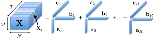
Figure 2: A rank-$R$ PARAFAC decomposition of the three-way tensor $\underline{\mathbf{X}}$.

The PARAFAC model is arguably the most basic tensor model because of its direct relationship to tensor rank. Based on the previous discussion it is natural to form a low-rank approximation of tensor $\underline{{\bf X}}\in\mathbb{R}^{M\times N\times T}$ as

$$\underline{{\bf X}}\approx\sum_{r=1}^{R}{\bf a}_{r}\circ{\bf b}_{r}\circ{\bf c}_{r}.$$ (15)

When the decomposition is exact, (15) is the PARAFAC decomposition of $\underline{{\bf X}}$; see also Fig. 2. Accordingly, the minimum value $R$ for which the exact decomposition is possible is (by definition) the rank of $\underline{{\bf X}}$. PARAFAC is the model of choice when one is primarily interested in revealing latent structure. Considering the analysis of a dynamic social network for instance, each of the rank-one factors in Fig. 2 could correspond to communities that e.g., persist or form and dissolve periodically across time. Different from the matrix case, there is no straightforward algorithm to determine the rank of a given tensor, a problem that has been shown to be NP-hard. For a survey of algorithmic approaches to obtain approximate PARAFAC decompositions, the reader is referred to [25].

With reference to (15), introduce the factor matrix ${\bf A}:=[{\bf a}_{1},\ldots,{\bf a}_{R}]\in\mathbb{R}^{M\times R}$, and likewise for ${\bf B}\in\mathbb{R}^{N\times R}$ and ${\bf C}\in\mathbb{R}^{T\times R}$. Let ${\bf X}_{t},\ t=1,\ldots,T$ denote the $t$-th slice of $\underline{{\bf X}}$ along its third (tube) dimension, such that ${\bf X}_{t}(m,n)=\underline{{\bf X}}(m,n,t)$; see also Fig. 2. The following compact matrix form of the PARAFAC decomposition in terms of slice factorizations will be used in the sequel

$${\bf X}_{t}={\bf A}{\rm diag}({\bm{\gamma}}_{t}){\bf B}^{\prime}=\sum_{r=1}^{R}{\bm{\gamma}}_{t}(r){\bf a}_{r}{\bf b}_{r}^{\prime},\quad t=1,2,\ldots,T$$ (16)

where ${\bm{\gamma}}_{t}^{\prime}$ denotes the $t$-th row of ${\bf C}$ (recall that ${\bf c}_{r}$ instead denotes the $r$-th column of ${\bf C}$). It is apparent that each slice ${\bf X}_{t}$ can be represented as a linear combination of $R$ rank-one matrices $\{{\bf a}_{r}{\bf b}_{r}^{\prime}\}_{r=1}^{R}$, which constitute the bases for the tensor fiber subspace. The PARAFAC decomposition is symmetric [cf. (15)], and one can likewise write ${\bf X}_{m}={\bf B}{\rm diag}({\bm{\alpha}}_{m}){\bf C}^{\prime}$, or, ${\bf X}_{n}={\bf C}{\rm diag}({\bm{\beta}}_{n}){\bf A}^{\prime}$ in terms of slices along the first (row), or, second (column) dimensions – once more, ${\bm{\alpha}}_{m}^{\prime}$ stands for the $m$-th row of ${\bf A}$, and likewise for ${\bm{\beta}}_{n}^{\prime}$. Given $\underline{\mathbf{X}}$, under some technical conditions then $\{{\bf A},{\bf B},{\bf C}\}$ are unique up to a common column permutation and scaling (meaning PARAFAC is identifiable); see e.g. [9, 26]

Building on the intuition for the matrix case, feasibility of the imputation task relies fundamentally on assuming a low-dimensional PARAFAC model for the data, to couple the available and missing entries as well as reduce the effective degrees of freedom in the problem. Under the low-rank assumption for instance, a rough idea on the fraction $p_{m}$ of missing data that can be afforded is obtained by comparing the number of unknowns $R(M+N+T)$ in (15) with the number of available data samples $(1-p_{m})MNT$. Ensuring that $(1-p_{m})MNT\geq R(M+N+T)$, roughly implies that the tensor can be potentially recovered even if a fraction $p_{m}\leq 1-R(M+N+T)/(MNT)$ of entries is missing. Different low-dimensional tensor models would lead to alternative imputation methods, such as the unfolded tensor regularization in [20, 28] for batch tensor completion. The algorithm in the following section offers (for the first time) an approach for decomposing and imputing low-rank streaming tensors.

V-B Algorithm for streaming tensor data

Let $\underline{{\bf Y}}\in\mathbb{R}^{M\times N\times T}$ be a three-way tensor, and likewise let $\underline{{\bf\Omega}}$ denote a $M\times N\times T$ binary $\{0,1\}$-tensor with $(m,n,t)$-th entry equal to $1$ if $\underline{{\bf Y}}(m,n,t)$ is observed, and $0$ otherwise. One can thus represent the incomplete data tensor compactly as $\mathcal{P}_{\underline{{\bf\Omega}}}(\underline{{\bf Y}})=\underline{{\bf\Omega}}\odot\underline{{\bf Y}}$; see also Fig. 3 (left). Generalizing the nuclear-norm regularization technique in (P1) from low-rank matrix to tensor completion is not straightforward if one also desires to unveil the latent structure in the data. The notion of singular values of a tensor (given by the Tucker3 decomposition) are not related to the rank [25]. Interestingly, it was argued in [7] that the Frobenius-norm regularization outlined in Section II-B offers a viable option for batch low-rank tensor completion under the PARAFAC model, by solving [cf. (P2) and (16)]

$${\rm(P4)}~{}~{}~{}~{}~{}\min_{\{{\bf X},{\bf A}\in\mathbbm{R}^{M\times\hat{R}},{\bf B}\in\mathbbm{R}^{N\times\hat{R}},{\bf C}\in\mathbbm{R}^{T\times\hat{R}}\}} \frac{1}{2}\|\underline{{\bf\Omega}}\odot(\underline{{\bf Y}}-\underline{{\bf X}})\|_{F}^{2}+\frac{\lambda}{2}(\|{\bf A}\|_{F}^{2}+\|{\bf B}\|_{F}^{2}+\|{\bf C}\|_{F}^{2})$$

$${\rm s.~{}to}~{}~{}{\bf X}_{t}={\bf A}{\rm diag}({\bm{\gamma}}_{t}){\bf B}^{\prime},\quad t=1,2\ldots,T.$$

The regularizer in (P4) provably encourages low-rank tensor decompositions, in fact with controllable rank by tuning the parameter $\lambda$ [7]. Note that similar to the matrix case there is no need for the true rank $R$ in (P4). In fact, any upperbound $\hat{R}\geq R$ can be used for the column size of the sought matrix variables ${\bf A},{\bf B},{\bf C}$ as long as $\lambda$ is tuned appropriately.

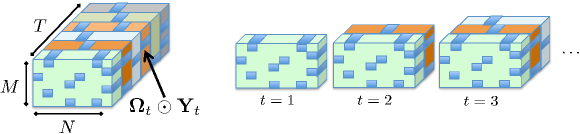
Figure 3: Tensor data with missing entries. (Left) Batch data, and slice $\bm{\Omega}_{t}\odot{\bf Y}_{t}$ along the time (tube) dimension. (Right) Streaming data, where slices $\bm{\Omega}_{t}\odot{\bf Y}_{t}$ become available for $t=1,2,\ldots$.

Consider now a real-time setting where the incomplete tensor slices $\bm{\Omega}_{t}\odot{\bf Y}_{t}$ are acquired sequentially over time $t=1,2,\ldots$ [i.e., streaming data as depicted in Fig. 3 (right)]. Leveraging the batch formulation (P4) one can naturally broaden the subspace tracking framework in Section III, to devise adaptive algorithms capable of factorizing tensors ‘on the fly’. To this end, one can estimate the PARAFAC model factors $\{{\bf A}[t],{\bf B}[t],{\bf C}[t]\}$ as the minimizers of the following EWLS cost [cf. (P3)]

$${\rm(P5)}~{}~{}\min_{\{{\bf A},{\bf B},{\bf C}\}}\frac{1}{2}\sum_{\tau=1}^{t}\theta^{t-\tau}\Big{[}\|{\bf\Omega}_{\tau}\odot({\bf Y}_{\tau}-{\bf A}{\rm diag}({\bm{\gamma}}_{\tau}){\bf B}^{\prime})\|_{F}^{2}+\bar{\lambda}_{t}(\|{\bf A}\|_{F}^{2}+\|{\bf B}\|_{F}^{2})+\lambda_{t}\|{\bm{\gamma}}_{\tau}\|^{2}\Big{]}.$$

Once more, the normalization $\bar{\lambda}:=\lambda_{t}/\sum_{\tau=1}^{t}\theta^{t-\tau}$ ensures that for the infinite memory setting ($\theta=1$) and $t=T$, (P5) coincides with the batch estimator (P4).

Paralleling the algorithmic construction steps adopted for the matrix case, upon defining the counterpart of $g_{t}({\bf L},{\bf q})$ corresponding to (P5) as

$$\bar{g}_{t}({\bf A},{\bf B},{\bm{\gamma}}):=\frac{1}{2}\|{\bf\Omega}_{t}\odot({\bf Y}_{t}-{\bf A}{\rm diag}({\bm{\gamma}}){\bf B}^{\prime})\|_{F}^{2}+\frac{\lambda_{t}}{2}\|{\bm{\gamma}}\|^{2}$$ (17)

the minimizer ${\bm{\gamma}}_{t}=\arg\min_{\bm{\gamma}}\bar{g}_{t}({\bf A},{\bf B},{\bm{\gamma}})$ is readily obtained in closed form, namely

$${\bm{\gamma}}_{t}=\left[\lambda{\bf I}_{R}+\sum_{(m,n)\in\Omega_{t}}({\bm{\alpha}}_{m}\odot{\bm{\beta}}_{n})({\bm{\alpha}}_{m}\odot{\bm{\beta}}_{n})^{\prime}\right]^{-1}\sum_{(m,n)\in\Omega_{t}}\underline{{\bf Y}}_{t}(m,n)({\bm{\alpha}}_{m}\odot{\bm{\beta}}_{n}).$$ (18)

Accordingly, the factor matrices $\{{\bf A},{\bf B}\}$ that can be interpreted as bases for the fiber subspace are the minimizers of the cost function

$$\bar{C}_{t}({\bf A},{\bf B}):=\sum_{\tau=1}^{t}\theta^{t-\tau}\bar{g}_{\tau}({\bf A},{\bf B},{\bm{\gamma}}_{\tau})+\frac{\bar{\lambda}_{t}}{2}(\|{\bf A}\|_{F}^{2}+\|{\bf B}\|_{F}^{2}).$$ (19)

Note that ${\bm{\gamma}}_{t}:={\bm{\gamma}}_{t}({\bf A},{\bf B})$ as per (18), so minimizing $\bar{C}_{t}({\bf A},{\bf B})$ becomes increasingly complex computationally as $t$ grows.

Remark 4 (Challenges facing a second-order algorithm)

As discussed in Section III, one can approximate $\bar{g}_{t}({\bf A},{\bf B},{\bm{\gamma}}_{t})$ with the upper bound $\bar{g}_{t}({\bf A},{\bf B},{\bm{\gamma}}_{t}({\bf A}[t-1],{\bf B}[t-1]))$ to develop a second-order algorithm that circumvents the aforementioned increasing complexity roadblock. Unlike the matrix case however, (19) is a nonconvex problem due to the bilinear nature of the PARAFAC decomposition (when, say, ${\bf C}$ is fixed); thus, finding its global optimum efficiently is challenging. One could instead think of carrying out alternating minimizations with respect to each of the tree factors per time instant $t$, namely updating: (i) ${\bm{\gamma}}[t]$ first, given $\{{\bf A}[t-1],{\bf B}[t-1]\}$; (ii) then ${\bf B}[t]$ given ${\bf A}[t-1]$ and $\{{\bm{\gamma}}[\tau]\}_{\tau=1}^{t}$; and (iii) finally ${\bf A}[t]$ with fixed ${\bf B}[t]$ and $\{{\bm{\gamma}}[\tau]\}_{\tau=1}^{t}$. While each of these subtasks boils down to a convex optimization problem, the overall procedure does not necessarily lead to an efficient algorithm since one can show that updating ${\bf A}[t]$ and ${\bf B}[t]$ recursively is impossible.

Acknowledging the aforementioned challenges and the desire of computationally-efficient updates compatible with Big Data requirements, it is prudent to seek instead a (first-order) SGD alternative. Mimicking the steps in Section III-B, let $\bar{f}_{t}({\bf A},{\bf B}):=\bar{g}_{t}({\bf A},{\bf B},{\bm{\gamma}}[t])+\frac{\lambda_{t}}{2t}(\|{\bf A}\|_{F}^{2}+\|{\bf B}\|_{F}^{2})$ denote the $t$-th summand in (19), for $t=1,2,\ldots$ and $\theta=1$. The factor matrices $\mathcal{L}[t]:=\{{\bf A}[t],{\bf B}[t]\}$ are obtained via the SGD iteration

$$\mathcal{L}[t]=\arg\min_{\mathcal{L}}\bar{Q}_{\bar{\mu}[t],t}(\mathcal{L},\mathcal{L}[t-1])=\mathcal{L}[t-1]-(\bar{\mu}[t])^{-1}\nabla\bar{f}_{t}(\mathcal{L}[t-1])$$ (20)

with the stepsize $(\bar{\mu}[t])^{-1}$, and $\bar{Q}_{\mu,t}(\mathcal{L}_{1},\mathcal{L}_{2}):=\bar{f}_{t}(\mathcal{L}_{2})+\langle\mathcal{L}_{1}-\mathcal{L}_{2},\nabla\bar{f}_{t}(\mathcal{L}_{2})\rangle+\frac{\mu}{2}\|\mathcal{L}_{1}-\mathcal{L}_{2}\|^{2}$. It is instructive to recognize that the quadratic surrogate $\bar{Q}_{\bar{\mu}[t],t}$ has the following properties: (i) it majorizes $\bar{f}_{t}(\mathcal{L})$, namely $\bar{f}_{t}(\mathcal{L})\leq\bar{Q}_{\bar{\mu},t}(\mathcal{L},\mathcal{L}[t-1]),~{}\forall\mathcal{L}$; while it is locally tight meaning that (ii) $\bar{f}_{t}(\mathcal{L}[t-1])=\bar{Q}_{\bar{\mu}[t],t}(\mathcal{L}[t-1],\mathcal{L}[t-1])$, and (iii) $\nabla\bar{f}_{t}(\mathcal{L}[t-1])=\nabla\bar{Q}_{\bar{\mu}[t],t}(\mathcal{L}[t-1],\mathcal{L}[t-1])$. Accordingly, the minimizer of $\bar{Q}_{\bar{\mu}[t],t}(\mathcal{L},\mathcal{L}[t-1])$ amounts to a correction along the negative gradient $\nabla\bar{f}_{t}(\mathcal{L}[t-1])$, with stepsize $(\bar{\mu}[t])^{-1}$ [cf. (20)].

Algorithm 3 : Online SGD algorithm for tensor decomposition and imputation

  input $\{{\bf Y}_{t},\bm{\Omega}_{t}\}_{t=1}^{\infty},$, $\{\bar{\mu}[t]\}_{t=1}^{\infty}$, $\hat{R}$, and $\lambda_{t}$.

  initialize $\{{\bf A}[0],{\bf B}[0]\}$ at random, and $\bar{\mu}[0]>0$.

  for $t=0,1,2$,$\ldots$ do

     ${\bf A}^{\prime}[t]:=[{\bm{\alpha}}_{1}[t],\ldots,{\bm{\alpha}}_{M}[t]]$ and ${\bf B}^{\prime}[t]:=[{\bm{\beta}}_{1}[t],\ldots,{\bm{\beta}}_{N}[t]]$

     ${\bm{\gamma}}[t]=\left[\lambda{\bf I}_{R}+\sum_{(m,n)\in\Omega_{t}}({\bm{\alpha}}_{m}[t]\odot{\bm{\beta}}_{n}[t])({\bm{\alpha}}_{m}[t]\odot{\bm{\beta}}_{n}[t])^{\prime}\right]^{-1}\sum_{(m,n)\in\Omega_{t}}{\bf Y}_{t}(m,n)({\bm{\alpha}}_{m}[t]\odot{\bm{\beta}}_{n}[t])$

     ${\bf A}[t+1]=(1-\frac{\lambda_{t}}{t\bar{\mu}[t]}){\bf A}[t]+\frac{1}{\bar{\mu}[t]}[{\bf\Omega}_{t}\odot({\bf Y}_{t}-{\bf A}[t]{\rm diag}({\bm{\gamma}}[t]){\bf B}^{\prime}[t])]{\bf B}[t]{\rm diag}({\bm{\gamma}}[t])$

     ${\bf B}[t+1]=(1-\frac{\lambda_{t}}{t\bar{\mu}[t]}){\bf B}[t]+\frac{1}{\bar{\mu}[t]}[{\bf\Omega}_{t}\odot({\bf Y}_{t}-{\bf A}[t]{\rm diag}({\bm{\gamma}}[t]){\bf B}^{\prime}[t])]^{\prime}{\bf A}[t]{\rm diag}({\bm{\gamma}}[t])$

  end for

  return  $\hat{{\bf X}}[t]:={\bf A}[t]{\rm diag}({\bm{\gamma}}[t]){\bf B}^{\prime}[t]$.

Putting together (18) and (20), while observing that the components of $\nabla\bar{f}_{t}(\mathcal{L})$ are expressible as

$$\nabla_{{\bf A}}\bar{f}_{t}({\bf A},{\bf B}) =-[{\bf\Omega}_{t}\odot({\bf Y}_{t}-{\bf A}{\rm diag}({\bm{\gamma}}[t]){\bf B}^{\prime})]{\bf B}{\rm diag}({\bm{\gamma}}[t])+\frac{\lambda_{t}}{t}{\bf A}$$ (21)

$$\nabla_{{\bf B}}\bar{f}_{t}({\bf A},{\bf B}) =-[{\bf\Omega}_{t}\odot({\bf Y}_{t}-{\bf A}{\rm diag}({\bm{\gamma}}[t]){\bf B}^{\prime})]^{\prime}{\bf A}{\rm diag}({\bm{\gamma}}[t])+\frac{\lambda_{t}}{t}{\bf B}$$ (22)

one arrives at the SGD iterations tabulated under Algorithm 3. Close examination of the recursions reveals that updating ${\bf A}[t]$ and ${\bf B}[t]$ demands $\mathcal{O}(|\Omega_{t}|\hat{R})$ operations, while updating ${\bm{\gamma}}[t]$ incurs a cost of $\mathcal{O}(|\Omega_{t}|\hat{R}^{2})$. The overall complexity per iteration is thus $\mathcal{O}(|\Omega_{t}|\hat{R}^{2})$.

Remark 5 (Forming the tensor decomposition ‘on-the-fly’)

In a stationary setting the low-rank tensor decomposition can be accomplished after the tensor subspace matrices are learned; that is, when the sequences $\{{\bf A}[t],{\bf B}[t]\}$ converge to the limiting points, say $\{\bar{{\bf A}},\bar{{\bf B}}\}$. The remaining factor $\bar{{\bf C}}:=[\bar{\bm{\gamma}}_{1}^{\prime},\ldots,\bar{\bm{\gamma}}_{T}^{\prime}]^{\prime}$ is then obtained by solving $\bar{\bm{\gamma}}_{t}=\arg\min_{\bm{\gamma}}\bar{g}_{t}(\bar{{\bf A}},\bar{{\bf B}},\bm{\gamma})$ for the corresponding tensor slice ${\cal P}_{\Omega_{t}}({\bf X}_{t})$, which yields a simple closed-form solution as in (18). This requires revisiting the past tensor slices. The factors $\{\bar{{\bf A}},\bar{{\bf B}},\bar{{\bf C}}\}$ then form a low-rank approximation of the entire tensor $\underline{{\bf X}}\in\mathbb{R}^{M\times N\times T}$. Note also that after the tensor subspace is learned say at time $t^{\prime}\leq T$, e.g., from some initial training data, the projection coefficients $\bar{\bm{\gamma}}_{t}$ can be calculated ‘on-the-fly’ for $t\geq t^{\prime}$; thus, Algorithm 3 offers a decomposition of then tensor containing slices $t^{\prime}$ to $t>t^{\prime}$ ‘on-the-fly’.

Convergence of Algorithm 3 is formalized in the next proposition, and can be established using similar arguments as in the matrix case detailed in Section IV-B. Furthermore, empirical observations in Section VI suggest that the convergence rate can be linear.

Proposition 4: Suppose slices $\{{\bf\Omega}_{t}\odot{\bf Y}_{t}\}_{t=1}^{\infty}$ and the corresponding sampling sets $\{\Omega_{t}\}_{t=1}^{\infty}$ are i.i.d., and $\theta=1$ while $\lambda_{t}=\lambda,~{}\forall t$. If (c1) $\{\mathcal{L}[t]\}_{t=1}^{\infty}$ live in a compact set, and (c2) the step-size sequence $\{(\bar{\mu}[t])^{-1}\}$ satisfies $\bar{\mu}[t]:=\sum_{\tau=1}^{t}\tilde{\alpha}[\tau]\geq ct,~{}\forall t$ for some $c>0$, where (c3) $c^{\prime}\geq\tilde{\alpha}[t]\geq\sigma_{\max}(\nabla^{2}\bar{f}_{t}(\mathcal{L}[t-1])),~{}\forall t$ for some $c^{\prime}>0$, then $\lim_{t\rightarrow\infty}\nabla C_{t}(\mathcal{L}[t])=\mathbf{0}$, a.s.; i.e., the tensor subspace iterates $\{\mathcal{L}[t]\}$ asymptotically coincide with the stationary points of (P4).

VI Numerical Tests

The convergence and effectiveness of the proposed algorithms is assessed in this section via computer simulations. Both synthetic and real data tests are carried out in the sequel.

VI-A Synthetic matrix data tests

The signal ${\bf x}_{t}={\bf U}{\bf w}_{t}$ is generated from the low-dimensional subspace ${\bf U}\in\mathbb{R}^{P\times r}$, with Gaussian i.i.d. entries $u_{p,i}\sim\mathcal{N}(0,1/P)$, and projection coefficients $w_{i,t}\sim\mathcal{N}(0,1)$. The additive noise $v_{i,t}\sim\mathcal{N}(0,\sigma^{2})$ is i.i.d., and to simulate the misses per time $t$, the sampling vector $\bm{\omega}_{t}\in\{0,1\}^{P}$ is formed, where each entry is a Bernoulli random variable, taking value one with probability (w.p.) $\pi$, and zero w.p. $1-\pi$, which implies that $(1-\pi)\times 100\%$ entries are missing. The observations at time $t$ are generated as $\mathcal{P}_{\omega_{t}}({\bf y}_{t})=\bm{\omega}_{t}\odot({\bf x}_{t}+{\bf v}_{t})$.

Throughout, fix $r=5$ and $\rho=10$, while different values of $\pi$ and $\sigma$ are examined. The time evolution of the average cost $C_{t}({\bf L}[t])$ in (10) for various amounts of misses and noise strengths is depicted in Fig. 4(a) [$\theta=1$]. For validation purposes, the optimal cost [normalized by the window size $t$] of the batch estimator (P1) is also shown. It is apparent that $C_{t}({\bf L}[t])$ converges to the optimal objective of the nuclear-norm regularized problem (P1), corroborating that Algorithm 1 attains the performance of (P1) in the long run. This observation in addition to the low cost of Algorithm 1 [$\mathcal{O}(|\omega_{t}|\rho^{2})$ per iteration] suggest it as a viable alternative for solving large-scale matrix completion problems.

Next, Algorithm 1 is compared with other state-of-the-art subspace trackers, including PETRELS [14] and GROUSE [4], discussed in Section I. In essence, these algorithms need the dimension of the underlying subspace, say $\kappa$, to be known/estimated a priori. Fix $\lambda=0.1$, $\theta=0.99$, and introduce an abrupt subspace change at time $t=10^{4}$ to assess the tracking capability of the algorithms. The figure of merit depicted in Fig. 4(b) is the running-average estimation error $e_{x}[t]:=\frac{1}{t}\sum_{i=1}^{t}\|\hat{{\bf x}}_{i}-{\bf x}_{i}\|_{2}/\|{\bf x}_{i}\|_{2}$. It is first observed that upon choosing identical subspace dimension $\kappa=\rho$ for all three schemes, Algorithm 1 attains a better estimation accuracy, where a constant step size $(\mu[t])^{-1}=0.1$ was adopted for PETRELS and GROUSE. Albeit PETRELS performs well when the true rank is known, namely $\kappa=r$, if one overestimates the rank the algorithm exhibits erratic behaviors for large fraction $75\%$ of missing observations. As expected, for the ideal choice of $\kappa=r$, all three schemes achieve nearly identical estimation accuracy. The smaller error exhibited by PETRELS relative to Algorithm 1 may pertain to the suboptimum selection of $\lambda$. Nonetheless, for large amount of misses both GROUSE and PETRELS are numerically unstable as the LS problems to obtain the projection coefficients ${\bf q}_{t}$ become ill-conditioned, whereas the ridge-regression type regularization terms in (P3) render Algorithm 1 numerically stable. The price paid by Algorithm 1 is however in terms of higher computational complexity per iteration, as seen in Table I which compares the complexity of various algorithms.

TABLE I: Computational complexity per iteration

.

GROUSE $(\kappa=\rho)$	PETRELS ($\kappa=\rho$)	Alg. 1 ($\theta\in(0,1)$)	Alg. 1 ($\theta=1$)	Alg. 2	Alg. 2 ($k[t]=1$)
$\mathcal{O}(P\rho+|\omega_{t}|\rho^{2})$	$\mathcal{O}(|\omega_{t}|\rho^{2})$	$\mathcal{O}(P\rho^{3})$	$\mathcal{O}(|\omega_{t}|\rho^{2})$	$\mathcal{O}(P\rho+|\omega_{t}|\rho^{2})$	$\mathcal{O}(|\omega_{t}|\rho^{2})$

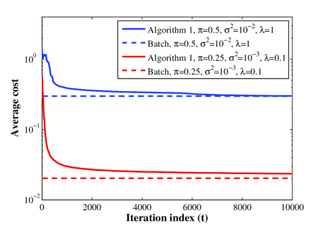
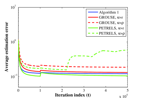
(a)	(b)

Figure 4: Performance of Algorithm 1. (a) Evolution of the average cost $C_{t}({\bf L}[t])$ versus the batch counterpart. (b) Relative estimation error for different schemes when $\pi=0.25$ and $\sigma^{2}=10^{-3}$.

VI-B Real matrix data tests

Accurate estimation of origin-to-destination (OD) flow traffic in the backbone of large-scale Internet Protocol (IP) networks is of paramount importance for proactive network security and management tasks [24]. Several experimental studies have demonstrated that OD flow traffic exhibits a low-intrinsic dimensionality, mainly due to common temporal patterns across OD flows, and periodic trends across time [27]. However, due to the massive number of OD pairs and the high volume of traffic, measuring the traffic of all possible OD flows is impossible for all practical purposes [27, 24]. Only the traffic level for a small fraction of OD flows can be measured via the NetFlow protocol [27].

Here, aggregate OD-flow traffic is collected from the operation of the Internet-2 network (Internet backbone across USA) during December 8-28, 2003 containing $121$ OD pairs [1]. The measured OD flows contain spikes (anomalies), which are discarded to end up with a anomaly-free data stream $\{{\bf y}_{t}\}\in\mathbb{R}^{121}$. The detailed description of the considered dataset can be found in [31]. A subset of entries of ${\bf y}_{t}$ are then picked randomly with probability $\pi$ to yield the input of Algorithm 1. The evolution of the running-average traffic estimation error ($e_{x}[t]$) is depicted in Fig. 5(a) for different schemes and under various amounts of missing data. Evidently, Algorithm 1 outperforms the competing alternatives when $\lambda_{t}$ is tuned adaptively as per Remark 2 for $\sigma^{2}=0.1$. When only $25\%$ of the total OD flows are sampled by Netflow, Fig. 5(b) depicts how Algorithm 1 accurately tracks three representative OD flows.

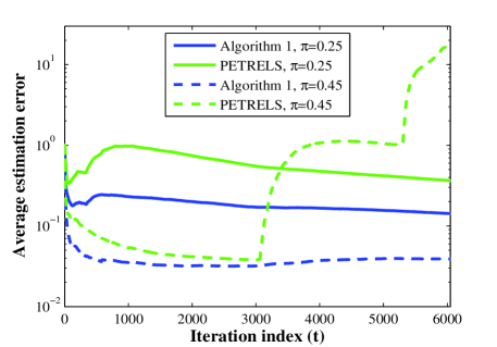
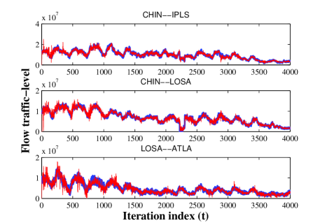
(a)	(b)

Figure 5: Traffic estimation performance for Internet-2 data when $\kappa=\rho=10$ and $\theta=0.95$. (a) Average estimation error for various amounts of missing data. (b) Algorithm 1’s estimated (red) versus true (blue) OD flow traffic for $75\%$ misses ($\pi=0.25$).

VI-C Synthetic tensor data tests

To form the $t$-th ‘ground truth’ tensor slice ${\bf X}_{t}={\bf A}{\rm diag}({\bm{\gamma}}_{t}){\bf B}^{\prime}\in\mathbb{R}^{M\times N}$, the factors ${\bf A}$ and ${\bf B}$ are generated independently with Gaussian i.i.d. columns ${\bf a}_{r}\sim{\cal N}(\mathbf{0},{\bf I}_{M})$ and ${\bf b}_{r}\sim{\cal N}(\mathbf{0},{\bf I}_{N})$; likewise, the coefficients ${\bm{\gamma}}_{t}\sim{\cal N}(0,{\bf I}_{R})$. The sampling matrix ${\bf\Omega}_{t}$ also contains random Bernoulli entries taking value one w.p. $\pi$, and zero w.p. $1-\pi$. Gaussian noise is also considered with i.i.d. entries ${\bf V}_{t}(m,n)\sim{\cal N}(0,\sigma^{2})$. Accordingly, the $t$-th acquired slice is formed as ${\bf Y}_{t}={\bf\Omega}_{t}\odot({\bf X}_{t}+{\bf V}_{t})$. Fix $\sigma=10^{-3}$ and the true rank $R=5$, while different values of $M,N,\hat{R},\pi$ are examined. Performance of Algorithm 3 is tested for imputation of streaming tensor slices of relatively large size $M=N=10^{3}$, where a constant step size $(\bar{\mu}[t])^{-1}=10^{-2}$ is adopted. Various amounts of misses are examined, namely $1-\pi\in\{0.99,0.9,0.75\}$. Also, in accordance with the matrix completion setup select $\lambda=\sqrt{2MN\pi}\sigma$; see e.g., [13]. Fig. 6 depicts the evolution of the estimation error $e_{x}[t]:=\|{\bf X}_{t}-\hat{{\bf X}}_{t}\|_{F}/\|{\bf X}_{t}\|_{F}$, where it is naturally seen that as more data become available the tensor subspace is learned faster. It is also apparent that after collecting sufficient amounts of data the estimation error decreases geometrically, where finally the estimate $\hat{{\bf X}}_{t}$ falls in the $\sigma^{2}$-neighborhood of the ‘ground truth’ slice ${\bf X}_{t}$. This observation suggests the linear convergence of Algorithm 3, and highlights the effectiveness of estimator (P3) in accurately reconstructing a large fraction of misses.

Here, Algorithm 3 is also adopted to decompose large-scale, dense tensors and hence find the factors $\hat{{\bf A}},\hat{{\bf B}},\hat{{\bf C}}$. For $T=10^{4}$ and for different slice sizes $M=N=10^{2}$ and $M=N=10^{3}$, the tensor may not even fit in main memory to apply batch solvers naively. After running Algorithm 3 instead, Table II reports the run-time under various amount of misses. One can see that smaller values of $\pi$ lead to shorter run-times since one needs to carry out less computations per iteration [c.f. $\mathcal{O}(|\Omega_{t}|\hat{R}^{2})$]. Note that the MATLAB codes for these experiments are by no means optimized, so further reduction in run-time is possible with a more meticulous implementation. Another observation is that for decomposition of low-rank tensors, it might be beneficial from a computational complexity standpoint to keep only a small subset of entries. Note that if instead of employing a higher-order decomposition one unfolds the tensor and resorts to the subspace tracking schemes developed in Section III for the sake of imputation, each basis vector entails $10^{6}$ variables. On the other hand, using tensor models each basis (rank-one) matrix entails only $2\times 10^{3}$ variables. Once again, for comparison purposes there is no alternative online scheme that imputes the missing tensor entries, and offers a PARAFAC tensor decomposition after learning the tensor subspace (see also Remark 5).

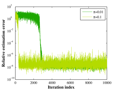
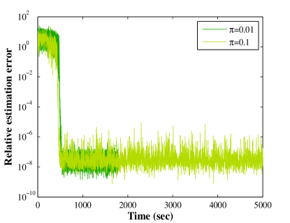
(a)	(b)

Figure 6: Relative estimation error versus (a) iterations and (b) run-time under various amounts of misses for $M=N=10^{3}$, $\sigma=10^{-3}$ and $R=10$.

TABLE II: Tensor imputation. Run-time (seconds) for various sizes and amounts of misses when $R=10$, $T=10^{4}$.

$M=N$	$\pi=0.01$	$\pi=0.1$	$\pi=0.25$
$10^{2}$	$26$	$132$	$302$
$10^{3}$	$1.8\times 10^{3}$	$10^{4}$	$3\times 10^{4}$

VI-D Real tensor data tests

Two real tensor data tests are carried out next, in the context of cardiac MRI and network traffic monitoring applications.

Cardiac MRI. Cardiac MRI nowadays serves as a major imaging modality for noninvasive diagnosis of heart diseases in clinical practice [19]. However, quality of MRI images is degraded as a result of fast acquisition process which is mainly due to patient’s breath-holding time. This may render some image pixels inaccurate or missing, and thus the acquired image only consists of a subset of pixels of the high-resolution ‘ground truth’ cardiac image. With this in mind, recovering the ‘ground truth’ image amounts to imputing the missing pixels. Low-rank tensor completion is well motivated by the low-intrinsic dimensionality of cardiac MRI images [21]. The FOURDIX dataset is considered for the ensuing tests, and contains $263$ cardiac scans with $10$ steps of the entire cardiac cycle [2]. Each scan is an image of size $512\times 512$ pixels, which is divided into $64$ patches of $32\times 32$ pixels. The $32\times 32$ patches then form slices of the tensor $\underline{{\bf X}}\in\mathbb{R}^{32\times 32\times 67,328}$. A large fraction ($75\%$ entries) of $\underline{{\bf X}}$ is randomly discarded to simulate missing data.

Imputing such a large, dense tensor via batch algorithms may be infeasible because of memory limitations. The online Algorithm 3 is however a viable alternative, which performs only $256\hat{R}^{2}$ operations on average per time step, and requires storing only $256+64\hat{R}$ variables. For a candidate image, the imputation results of Algorithm 3 are depicted in Fig. 7 for different choices of the rank $\hat{R}=10,50$. A constant step size $(\bar{\mu}[t])^{-1}=10^{-6}$ is chosen along with $\lambda=0.01$. Different choices of the rank $\hat{R}=10,50$ lead to $e_{x}=0.14,0.046$, respectively. Fig. 7(a) shows the ‘ground truth’ image, while Fig. 7(b) depicts the acquired one with only $25\%$ available (missing entries are set to zero for display purposes.) Fig. 7(c) also illustrates the reconstructed image after learning the tensor subspace for $\hat{R}=10$, and the result for $\hat{R}=50$ is shown in Fig. 7(d). Note that although this test assumes misses in the spatial domain, it is more natural to consider misses in the frequency domain, where only a small subset of DFT coefficients are available. This model can be captured by the estimator (P5), by replacing the fidelity term with $\|{\bf\Omega}_{\tau}\odot\Psi({\bf Y}_{\tau}-{\bf A}{\rm diag}({\bm{\gamma}}_{\tau}){\bf B}^{\prime})\|_{F}^{2}$, where $\Psi$ stands for the linear Fourier operator.

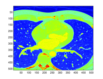
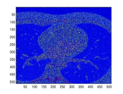
(a)	(b)
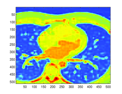
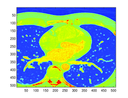
(c)	(d)

Figure 7: Results of applying Algorithm 3 to the cardiac MRI dataset FOURDIX [2]. (a) Ground truth image, (b) acquired image with $75\%$ missing pixels, and the reconstructed image for rank (c) $\hat{R}=10$ and (d) $\hat{R}=50$.

Tracking network-traffic anomalies. In the backbone of large-scale IP networks, OD flows experience traffic volume anomalies due to e.g., equipment failures and cyberattacks which can congest the network [41]. Consider a network whose topology is represented by a directed graph $G(\mathcal{N},\mathcal{L})$, where $\mathcal{L}$ and $\mathcal{N}$ denote the set of links and nodes of cardinality $|\mathcal{L}|=L$ and $|\mathcal{N}|=N$, respectively. Upon associating the weight $w_{i,j}>0,~{}(i,j)\in E$ with the $(i,j)$-th link, $G$ can be completely described by the weighted adjacency matrix ${\bf W}\in\mathbb{R}^{N\times N}$. For instance $w_{i,j}$ can represent the link loads as will be shown later. In the considered network, a set of OD traffic flows $\mathcal{F}$ with $|\mathcal{F}|=F$ traverses the links connecting OD pairs. Let $r_{\ell,f}\in[0,1]$ denote the fraction of $f$-th flow traffic at time $t$, say $x_{f,t}$, measured in e.g., packet counts, carried by link $\ell$. The overall traffic carried by link $\ell$ is then the superposition of the flow rates routed through link $\ell$, namely, $\sum_{f\in\mathcal{F}}r_{\ell,f}x_{\ell,f}$. It is not uncommon for some of OD flows to experience anomalies. If $o_{f,t}$ denotes the unknown traffic volume anomaly of flow $f$ at time $t$, the measured link counts over link $\ell$ at time $t$ are then given by

$$y_{\ell,t}=\sum_{f\in\mathcal{F}}r_{\ell,f}(x_{f,t}+o_{f,t})+v_{\ell,t},~{}\ell\in\mathcal{L}$$ (23)

where $v_{\ell,t}$ accounts for measurement errors and unmodeled dynamics. In practice, missing link counts are common due to e.g., packet losses, and thus per time only a small fraction of links (indexed by $\Omega_{t}$) are measured. Note that only a small group of flows are anomalous, and the anomalies persist for short periods of time relative to the measurement horizon. This renders the anomaly vector ${\bf o}_{t}=[o_{1,t},\ldots,o_{F,t}]^{\prime}\in\mathbb{R}^{F}$ sparse.

In general, one can collect the partial link counts per time instant in a vector to form a (vector-valued) time-series, and subsequently apply the subspace tracking algorithms developed in e.g., [31] to unveil the anomalies in real time. Instead, to fully exploit the data structure induced by the network topology, the link counts per time $t$ can be collected in an adjacency matrix ${\bf W}_{t}$, with $[{\bf W}_{t}]_{i,j}=y_{\ell,t}$ [edge $(i,j)$ corresponds to link $\ell$]. This matrix naturally constitutes the $t$-th slice of the tensor $\underline{{\bf Y}}$. Capitalizing on the spatiotemporal low-rank property of the nominal traffic as elaborated in Section VI-B, to discern the anomalies a low-rank ($\rho\ll R$) approximation of the incomplete tensor $\underline{{\bf\Omega}}\odot\underline{{\bf Y}}$ is obtained first in an online fashion using Algorithm 3. Anomalies are then unveiled from the residual of the approximation as elaborated next.

Let $\{{\bf A}[t],{\bf B}[t]\}$ denote the factors of the low-dimensional tensor subspace learned at time $t$, and $\hat{{\bf Y}}_{t}={\bf A}[t]{\rm diag}({\bm{\gamma}}[t]){\bf B}^{\prime}[t]\in\mathbb{R}^{N\times N}$ the corresponding (imputed) low-rank approximation of the $t$-th slice. Form the residual matrix $\tilde{{\bf Y}}_{t}:={\bf Y}_{t}-\hat{{\bf Y}}_{t}$, which is (approximately) zero in the absence of anomalies. Collect the nonzero entries of $\tilde{{\bf Y}}_{t}$ into the vector $\tilde{{\bf y}}_{t}\in\mathbb{R}^{L}$, and the routing variables $r_{\ell,f}$ [cf. (23)] into matrix ${\bf R}\in\mathbb{R}^{L\times F}$. According to (23), one can postulate the linear regression model $\tilde{{\bf y}}_{t}={\bf R}{\bf o}_{t}+{\bf v}_{t}$ to estimate the sparse anomaly vector ${\bf o}_{t}\in\mathbb{R}^{F}$ from the imputed link counts. An estimate of ${\bf o}_{t}$ can then be obtained via the least-absolute shrinkage and selection operator (LASSO)

$$\hat{{\bf o}}_{t}:=\arg\min_{{\bf o}\in\mathbb{R}^{F}}\|\tilde{{\bf y}}_{t}-{\bf R}{\bf o}\|^{2}+\lambda_{o}\|{\bf o}\|_{1}$$

where $\lambda_{o}$ controls the sparsity in $\hat{{\bf o}}_{t}$ that is tantamount to the number of anomalies. In the absence of missing links counts, [23] has recently considered a batch tensor model of link traffic data and its Tucker decomposition to identify the anomalies.

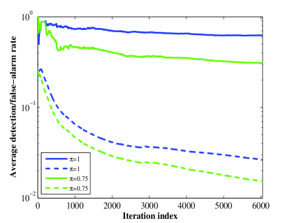
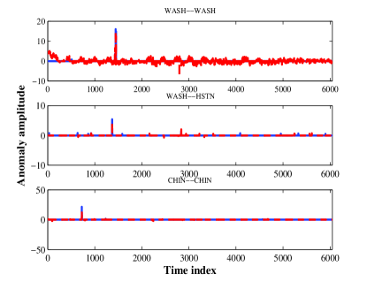
(a)	(b)

Figure 8: Tracking Internet-2 traffic anomalies for $\rho=18$. (a) Evolution of average detection (solid) and false-alarm (dashed) rates. (b) Estimated (red) versus true (blue) anomalies for three representative OD flows when $\pi=1$.

The described tensor-based approach for network anomaly detection is tested on the Internet-2 traffic dataset described in Section VI-B, after fixing $\hat{R}=18$. Each tensor slice ${\bf Y}_{t}\in\mathbb{R}^{11\times 11}$ contains only $41$ nonzero entries corresponding to the physical links. Define the sets $S_{O}[t]:=\{(i,j),~{}i\in[L],j\in[t]:~{}|o_{j}(i)|\geq\xi\}$ and $\bar{S}_{O}[t]:=\{(i,j),~{}i\in[L],j\in[t]:~{}|o_{j}(i)|\leq\xi\}$ for some prescribed threshold $\xi$. To evaluate the detection performance, the adopted figures of merit are the running-average detection and false-alarm rates $P_{\rm D}:=|S_{O}\cap S_{\hat{O}}|/|S_{O}|$ and $P_{\rm FA}:=|\bar{S}_{O}\cap S_{\hat{O}}|/|\bar{S}_{O}|$, respectively. Fig. 8(a) depicts the time evolution of $P_{\rm D}$ and $P_{\rm FA}$ for $\pi=1$ (fully available data), and $\pi=0.75$. As more data becomes available, the traffic subspace is learned more accurately, and thus less false alarms are declared. For three representative OD flows, namely WASH-WASH, WASH–HSTN, and CHIN–CHIN, the true and estimated anomalies are depicted in Fig. 8(b). One can see that the significant anomalies are correctly picked in real-time by the proposed estimator. Note that the online formulation (P5) can even accommodate slowly-varying network topologies in the tensor model, which is desirable for monitoring the ‘health state’ of dynamic networks.

VII Concluding Summary

This paper leverages recent advances in rank minimization for subspace tracking, and puts forth streaming algorithms for real-time, scalable decomposition of highly-incomplete multi-way Big Data arrays. For low-rank matrix data, a subspace tracker is developed based on an EWLS criterion regularized with the nuclear norm. Leveraging a separable characterization of nuclear-norm, both first- and second-order algorithms with complementary strengths are developed. In a stationary setting, the proposed algorithms asymptotically converge and provably offer the well-documented performance guarantees of the batch nuclear-norm regularized estimator. Under the same umbrella, an online algorithm is proposed for decomposing low-rank tensors with missing entries, which can accurately impute cardiac MRI images with up to $75\%$ missing entries.

There are intriguing unanswered questions beyond the scope of this paper, but worth pursuing as future research. One such question pertains to the convergence analysis of the accelerated SGD algorithm either by following the adopted proof methodology, or, e.g., the alternative techniques used in [36]. Real-time incorporation of the spatiotemporal correlation between the unknowns by means of kernels or suitable statistical models is another important avenue to explore. Also, relaxing the qualification constraint for optimality is important for real-time applications in dynamic environments, where the learned subspace could conceivably change with time.

Proof of Proposition IV-C. For the subspace sequence $\{{\bf L}[t]\}$ suppose that $\lim_{t\rightarrow\infty}\nabla C_{t}({\bf L}[t])=\mathbf{0}$. Then, due to the uniqueness of ${\bf q}[t]=\arg\min_{{\bf q}}g_{t}({\bf L}[t],{\bf q})$, Danskin’s Theorem [10] implies that

$$\lim_{t\rightarrow\infty}\frac{1}{t}\left(\mathcal{P}_{\Omega_{t}}({\bf Y}_{t}-{\bf L}[t]{\bf Q}^{\prime}[t]){\bf Q}[t]-\lambda{\bf L}[t]\right)=\mathbf{0}$$ (24)

holds true almost surely, where ${\bf Q}[t]\in\mathbb{R}^{P\times t}$ satisfies

$${\bf L}^{\prime}[t]\mathcal{P}_{\Omega_{t}}({\bf Y}_{t}-{\bf L}[t]{\bf Q}^{\prime}[t])-\lambda{\bf Q}^{\prime}[t]=\mathbf{0}.$$ (25)

Consider now a subsequence $\{{\bf L}[t_{k}],{\bf Q}[t_{k}]\}_{k=1}^{\infty}$ which satisfies (24)–(25) as well as the qualification constraint $\|\mathcal{P}_{\Omega_{t_{k}}}({\bf Y}_{t_{k}}-{\bf L}[t_{k}]{\bf Q}^{\prime}[t_{k}])\|\leq\lambda$. The rest of the proof then verifies that $\{{\bf L}[t_{k}],{\bf Q}[t_{k}]\}$ asymptotically fulfills the optimality conditions for (P1). To begin with, the following equivalent formulation of (P1) is considered at time $t_{k}$, which no longer involves the non-smooth nuclear norm.

$$\text{(P5)}~{}~{}~{}\min_{\begin{subarray}{c}\{{\bf X}\in\mathbb{R}^{P\times P},{\bf W}_{1}\in\mathbb{R}^{P\times t_{k}}\\ {\bf W}_{2}\in\mathbb{R}^{t_{k}\times t_{k}}\}\end{subarray}} \left[\frac{1}{2t_{k}}\|\mathcal{P}_{\Omega_{t_{k}}}({\bf Y}_{t_{k}}-{\bf X})\|_{F}^{2}+\frac{\lambda}{2t_{k}}\left\{\text{tr}({\bf W}_{1})+\text{tr}({\bf W}_{2})\right\}\right]$$

s. to $${\bf W}:=\left(\begin{array}[]{cc}{\bf W}_{1}&{\bf X}\\ {\bf X}^{\prime}&{\bf W}_{2}\end{array}\right)\succeq\mathbf{0}$$ (28)

To explore the optimality conditions for (P5), first form the Lagrangian

$$\mathcal{L}_{t_{k}}({\bf X},{\bf W}_{1},{\bf W}_{2};{\bf M})=\frac{1}{2t_{k}}\|\mathcal{P}_{\Omega_{t_{k}}}({\bf Y}_{t_{k}}-{\bf X})\|_{F}^{2}+\frac{\lambda}{2t_{k}}\left(\text{tr}\{{\bf W}_{1}\}+\text{tr}\{{\bf W}_{2}\}\right)-\langle{\bf M},{\bf W}\rangle.$$ (29)

where ${\bf M}$ denotes the dual variables associated with the positive semi-definiteness constraint in (P5). For notational convenience, partition ${\bf M}$ into four blocks, namely ${\bf M}_{1}:=[{\bf M}]_{11}$, ${\bf M}_{2}:=[{\bf M}]_{12}$, ${\bf M}_{3}:=[{\bf M}]_{22}$, and ${\bf M}_{4}:=[{\bf M}]_{21}$, in accordance with the block structure of ${\bf W}$ in (P5), where ${\bf M}_{1}$ and ${\bf M}_{3}$ are $P\times P$ and $t_{k}\times t_{k}$ matrices. The optimal solution to (P1) must: (i) null the (sub)gradients

$$\nabla_{{\bf X}}{\mathcal{L}}_{t_{k}}({\bf X},{\bf W}_{1},{\bf W}_{2};{\bf M})=-\frac{1}{t_{k}}\mathcal{P}_{\Omega_{t_{k}}}({\bf Y}_{t_{k}}-{\bf X})-{\bf M}_{2}-{\bf M}^{\prime}_{4}$$ (30)

$$\nabla_{{\bf W}_{1}}{\mathcal{L}}_{t_{k}}({\bf X},{\bf W}_{1},{\bf W}_{2};{\bf M})=\frac{\lambda}{2t_{k}}{\bf I}_{L}-{\bf M}_{1}$$ (31)

$$\nabla_{{\bf W}_{2}}{\mathcal{L}}_{t_{k}}({\bf X},{\bf W}_{1},{\bf W}_{2};{\bf M})=\frac{\lambda}{2t_{k}}{\bf I}_{t_{k}}-{\bf M}_{3}$$ (32)

(ii) satisfy the complementary slackness condition $\langle{\bf M},{\bf W}\rangle=0$; (iii) primal feasibility ${\bf W}\succeq\mathbf{0}$; and (iv) dual feasibility ${\bf M}\succeq\mathbf{0}$.

Introduce the candidate primal variables ${\bf X}[k]:={\bf L}[t_{k}]{\bf Q}^{\prime}[t_{k}]$, ${\bf W}_{1}[k]:={\bf L}[t_{k}]{\bf L}^{\prime}[t_{k}]$ and ${\bf W}_{2}[k]:={\bf Q}[t_{k}]{\bf Q}^{\prime}[t_{k}]$; and the dual variables ${\bf M}_{1}[k]:=\frac{\lambda}{2t_{k}}{\bf I}_{L}$, ${\bf M}_{3}[k]:=\frac{\lambda}{2t_{k}}{\bf I}_{t}$, ${\bf M}_{2}[k]:=-(1/2t_{k})\mathcal{P}_{\Omega_{t_{k}}}({\bf Y}_{t_{k}}-{\bf L}[t_{k}]{\bf Q}^{\prime}[t_{k}])$, and ${\bf M}_{4}[k]:={\bf M}_{2}^{\prime}[k]$. Then, it can be readily verified that (i), (iii) and (iv) hold. Moreover, (ii) holds since

$$\langle{\bf M}[k],{\bf W}[k]\rangle =\langle{\bf M}_{1}[k],{\bf W}_{1}[k]\rangle+\langle{\bf M}_{2}[k],{\bf X}[k]\rangle+\langle{\bf M}_{2}^{\prime}[k],{\bf X}^{\prime}[k]\rangle+\langle{\bf M}_{3}[k],{\bf W}_{2}[k]\rangle$$

$$=\frac{\lambda}{2t_{k}}\langle{\bf I}_{L},{\bf L}[t_{k}]{\bf L}^{\prime}[t_{k}]\rangle+\frac{\lambda}{2t_{k}}\langle{\bf I}_{t_{k}},{\bf Q}[t_{k}]{\bf Q}^{\prime}[t_{k}]\rangle-\frac{1}{t_{k}}\langle\mathcal{P}_{\Omega_{t_{k}}}({\bf Y}_{t_{k}}-{\bf L}[t_{k}]{\bf Q}^{\prime}[t_{k}]),{\bf L}[t_{k}]{\bf Q}^{\prime}[t_{k}]\rangle$$

$$=\frac{1}{2t_{k}}\langle{\bf L}[t_{k}],\lambda{\bf L}[t_{k}]-\mathcal{P}_{\Omega_{t_{k}}}({\bf Y}_{t_{k}}-{\bf L}[t_{k}]{\bf Q}^{\prime}[t_{k}]){\bf Q}[t_{k}]\rangle$$

$$\hskip 113.81102pt+\frac{1}{2t_{k}}\langle{\bf Q}^{\prime}[t_{k}],\lambda{\bf Q}^{\prime}[t_{k}]-{\bf L}^{\prime}[t_{k}]\mathcal{P}_{\Omega_{t_{k}}}({\bf Y}_{t_{k}}-{\bf L}[t_{k}]{\bf Q}^{\prime}[t_{k}])\rangle$$

$$=\frac{1}{2t_{k}}\langle{\bf L}[t_{k}],\lambda{\bf L}[t_{k}]-\mathcal{P}_{\Omega_{t_{k}}}({\bf Y}_{t_{k}}-{\bf L}[t_{k}]{\bf Q}^{\prime}[t_{k}]){\bf Q}[t_{k}]\rangle$$

where the last equality is due to (25). Putting pieces together, the Cauchy-Schwartz inequality implies that

$$\lim_{k\rightarrow\infty}|\langle{\bf M}[k],{\bf W}[k]\rangle|\leq\sup_{k}\|{\bf L}[t_{k}]\|_{F}$$

$$\hskip 56.9055pt\times\lim_{k\rightarrow\infty}\|\frac{1}{2t_{k}}\left(\lambda{\bf L}[t_{k}]-\mathcal{P}_{\Omega_{t_{k}}}({\bf Y}_{t_{k}}-{\bf L}[t_{k}]{\bf Q}^{\prime}[t_{k}]){\bf Q}[t_{k}]\right)\|_{F}\ =0$$

holds almost surely due to (24), and (A3) which says $\|{\bf L}[t_{k}]\|_{F}$ is bounded. All in all, $\lim_{k\rightarrow\infty}\langle{\bf M}[k],{\bf W}[k]\rangle=0$, which completes the proof. $\blacksquare$

References

- [1] [Online]. Available: http://internet2.edu/observatory/archive/data-collections.html
- [2] [Online]. Available: http://http://www.osirix-viewer.com/datasets.
- [3] E. Acar, D. M. Dunlavy, T. G. Kolda, and M. Mørup, “Scalable tensor factorizations for incomplete data,” Chemometrics and Intelligent Laboratory Systems, vol. 106, no. 1, pp. 41–56, 2011.
- [4] L. Balzano, R. Nowak, and B. Recht, “Online identification and tracking of subspaces from highly incomplete information,” in Proc. of Allerton Conference on Communication, Control, and Computing, Monticello, USA, Jun. 2010.
- [5] L. Balzano, “On GROUSE and incremental SVD,” in Proc. of 5th Workshop on Comp. Advances in Multi-Sensor Adaptive Proc., St. Martin, Dec. 2013.
- [6] L. Balzano and S. J. Wright, “Local convergence of an algorithm for subspace identification from partial data.” Submitted for publication. Preprint available at http://arxiv.org/abs/1306.3391.
- [7] J. A. Bazerque, G. Mateos, and G. B. Giannakis, “Rank regularization and Bayesian inference for tensor completion and extrapolation,” IEEE Trans. Signal Process., vol. 61, no. 22, pp. 5689–5703, nov 2013.
- [8] A. Beck and M. Teboulle, “A fast iterative shrinkage-thresholding algorithm for linear inverse problems,” SIAM J. Imag. Sci., vol. 2, pp. 183–202, Jan. 2009.
- [9] J. M. F. T. Berge and N. D. Sidiropoulos, “On uniqueness in CANDECOMP/PARAFAC,” Psychometrika, vol. 67, no. 3, pp. 399–409, 2002.
- [10] D. P. Bertsekas, Nonlinear Programming, 2nd ed. Athena-Scientific, 1999.
- [11] S. Burer and R. D. Monteiro, “Local minima and convergence in low-rank semidefinite programming,” Mathematical Programming, vol. 103, no. 3, pp. 427–444, 2005.
- [12] E. J. Candes and B. Recht, “Exact matrix completion via convex optimization,” Found. Comput. Math., vol. 9, no. 6, pp. 717–722, 2009.
- [13] E. Candes and Y. Plan, “Matrix completion with noise,” Proceedings of the IEEE, vol. 98, pp. 925–936, 2009.
- [14] Y. Chi, Y. C. Eldar, and R. Calderbank, “PETRELS: Subspace estimation and tracking from partial observations,” in Proc. of IEEE Int. Conf. on Acoustics, Speech and Signal Process., Kyoto, Japan, Mar. 2012.
- [15] ——, “PETRELS: Parallel subspace estimation and tracking using recursive least squares from partial observations,” IEEE Trans. Signal Process., vol. 61, no. 23, pp. 5947–5959, 2013.
- [16] W. Dai, O. Milenkovic, and E. Kerman, “Subspace evolution and transfer (SET) for low-rank matrix completion,” IEEE Trans. Signal Process., vol. 59, no. 7, pp. 3120–3132, July 2011.
- [17] M. Fazel, “Matrix rank minimization with applications,” Ph.D. dissertation, Stanford University, 2002.
- [18] J. Feng, H. Xu, and S. Yan, “Online robust PCA via stochastic optimization,” in Proc. Advances in Neural Information Processing Systems, Lake Tahoe, NV, Dec. 2013.
- [19] J. Finn, K. Nael, V. Deshpande, O. Ratib, and G. Laub, “Cardiac MR imaging: State of the technology,” Radiology, vol. 241, no. 2, pp. 338–354, 2006.
- [20] S. Gandy, B. Recht, and I. Yamada, “Tensor completion and low-n-rank tensor recovery via convex optimization,” Inverse Problems, vol. 27, no. 2, pp. 1–19, 2011.
- [21] H. Gao, “Prior rank, intensity and sparsity model (PRISM): a divide-and-conquer matrix decomposition model with low-rank coherence and sparse variation,” in Proc. of SPIE Optical Engineering Applications, 2012.
- [22] T. Hastie, R. Tibshirani, and J. Friedman, The Elements of Statistical Learning, 2nd ed. Springer, 2009.
- [23] H. Kim, S. Lee, X. Ma, and C. Wang, “Higher-order PCA for anomaly detection in large-scale networks,” in Proc. of 3rd Workshop on Comp. Advances in Multi-Sensor Adaptive Proc., Aruba, Dutch Antilles, Dec. 2009.
- [24] E. D. Kolaczyk, Statistical Analysis of Network Data: Methods and Models. Springer, 2009.
- [25] T. G. Kolda and B. W. Bader, “Tensor decompositions and applications,” SIAM Review, vol. 51, no. 3, pp. 455–500, 2009.
- [26] J. Kruskal, “Three-way arrays: Rank and uniqueness of trilinear decompositions with application to arithmetic complexity and statistics,” Lin. Alg. Applications, vol. 18, no. 2, pp. 95–138, 1977.
- [27] A. Lakhina, K. Papagiannaki, M. Crovella, C. Diot, E. D. Kolaczyk, and N. Taft, “Structural analysis of network traffic flows,” in Proc. of ACM SIGMETRICS, New York, NY, Jul. 2004.
- [28] J. Liu, P. Musialski, P. Wonka, and J. Ye, “Tensor completion for estimating missing values in visual data,” IEEE Trans. Pattern Analysis and Machine Intelligence, vol. 35, pp. 208–220, Jan. 2013.
- [29] J. Mairal, F. Bach, J. Ponce, and G. Sapiro, “Online learning for matrix factorization and sparse coding,” J. of Machine Learning Research, vol. 11, pp. 19–60, Jan. 2010.
- [30] M. Mardani, G. Mateos, and G. B. Giannakis, “Decentralized sparsity regularized rank minimization: Applications and algorithms,” IEEE Trans. Signal Process., vol. 61, pp. 5374–5388, Nov. 2013.
- [31] ——, “Dynamic anomalography: tracking network anomalies via sparsity and low rank,” IEEE J. Sel. Topics in Signal Process., vol. 7, no. 11, pp. 50–66, Feb. 2013.
- [32] Y. Nesterov, “A method of solving a convex programming problem with convergence rate ,” Soviet Mathematics Doklady, vol. 27, pp. 372–376, 1983.
- [33] D. Nion and N. D. Sidiropoulos, “Adaptive algorithms to track the PARAFAC decomposition of a third-order tensor,” IEEE Trans. Signal Process, vol. 57, no. 6, pp. 2299–2310, 2009.
- [34] B. Recht, M. Fazel, and P. A. Parrilo, “Guaranteed minimum-rank solutions of linear matrix equations via nuclear norm minimization,” SIAM Rev., vol. 52, no. 3, pp. 471–501, 2010.
- [35] M. Signoretto, R. V. Plas, B. D. Moor, and J. A. K. Suykens, “Tensor versus matrix completion: A comparison with application to spectral data,” IEEE Signal Processing Letters, vol. 18, pp. 403–406, 2011.
- [36] K. Slavakis and G. B. Giannakis, “Online dictionary learning from big data using accelerated stochastic approximation algorithms,” in Proc. Intl. Conf. on Acoustic Speech and Signal Process., Florence, Italy, May 2014.
- [37] K. Slavakis, G. B. Giannakis, and G. Mateos, “Modeling and optimization for Big Data analytics,” IEEE Signal Process. Mag., vol. 31, no. 5, 2014 (to appear).
- [38] V. Solo and X. Kong, Adaptive Signal Processing Algorithms: Stability and Performance. Prentice Hall, 1995.
- [39] P. Sprechmann, A. M. Bronstein, and G. Sapiro, “Real-time online singing voice separation from monaural recordings using robust low-rank modeling,” in Proc. Annual Conference of the Intl. Society for Music Info. Retrieval, Porto, Portugal, Oct. 2012.
- [40] N. Srebro and A. Shraibman, “Rank, trace-norm and max-norm,” in Proc. of Learning Theory. Springer, 2005, pp. 545–560.
- [41] M. Thottan and C. Ji, “Anomaly detection in IP networks,” IEEE Trans. Signal Process., vol. 51, pp. 2191–2204, Aug. 2003.
- [42] B. Yang, “Projection approximation subspace tracking,” IEEE Trans. Signal. Process., vol. 43, pp. 95–107, Jan. 1995.
- [43] J. F. Yang and M. Kaveh, “Adaptive eigensubspace algorithms for direction or frequency estimation and tracking,” IEEE Trans. Acoust., Speech, Signal Process., vol. 36, no. 2, pp. 241–251, 1988.