Quantile Spectral Analysis
for Locally Stationary Time Series

Abstract

Classical spectral methods are subject to two fundamental limitations: they only can account for covariance-related serial dependencies, and they require second-order stationarity. Much attention has been devoted lately to quantile-based spectral methods that go beyond covariance-based serial dependence features. At the same time, covariance-based methods relaxing stationarity into much weaker local stationarity conditions have been developed for a variety of time-series models. Here, we are combining those two approaches by proposing quantile-based spectral methods for locally stationary processes. We therefore introduce a time-varying version of the copula spectra that have been recently proposed in the literature, along with a suitable local lag-window estimator. We propose a new definition of local strict stationarity that allows us to handle completely general non-linear processes without any moment assumptions, thus accommodating our quantile-based concepts and methods. We establish a central limit theorem for the new estimators, and illustrate the power of the proposed methodology by means of a simulation study. Moreover, in two empirical studies (namely of the Standard & Poor’s 500 series and a temperature dataset recorded in Hohenpeissenberg) we demonstrate that the new approach detects important variations in serial dependence structures both across time and across quantiles. Such variations remain completely undetected, and are actually undetectable, via classical covariance-based spectral methods.

AMS 1980 subject classification : 62M15, 62G35.

Key words and phrases : Copulas, Nonstationarity, Ranks, Periodogram, Laplace spectrum.

1 Introduction

For more than a century, spectral methods have been among the favorite tools of time-series analysis. The concept of periodogram was proposed and discussed as early as 1898 by Schuster, who coined the term in a study (Schuster, (1898)) of meteorological series. The modern mathematical foundations of the approach were laid between 1930 and 1950 by such big names as Wiener, Cramér, Kolmogorov, Bartlett, and Tukey. The main reason for the unwavering success of spectral methods is that they are entirely model-free, hence fully nonparametric; as such, they can be considered a precursor to the subsequent development of nonparametric techniques in the area and, despite their age, they still are part of the leading group of methods in the field.

The classical spectral approach to time series analysis, however, remains deeply marked by two major restrictions:

(i)

as a second-order theory, it is essentially limited to modeling first- and second-order dynamics: being entirely covariance-based, it cannot accommodate heavy tails and infinite variances, and cannot account for any dynamics in conditional skewness, kurtosis, or tail behavior;

(ii)

the assumption of second-order stationarity is pervasive: except for processes that, possibly after some adequate transformation such as differencing or cointegration, are second-order stationary, observations exhibiting time-varying distributional features are ruled out.

The first of these two limitations recently has attracted much attention, and new quantile-related spectral analysis tools have been proposed, which do not require second-order moments, and are able to capture serial features that cannot be accounted for by the classical second-order approach. Pioneering contributions in that direction are Hong, (1999) and Li, (2008), who coined the names of Laplace spectrum and Laplace periodogram. The Laplace spectrum concept was further studied by Hagemann, (2013), and extended into cross-spectrum and spectral kernel concepts by Dette et al., (2015), who also introduced copula-based versions of the same. Those copula spectral quantities are indexed by couples $(\tau_{1},\tau_{2})$ of quantile levels, and their collections (for $(\tau_{1},\tau_{2})\in[0,1]^{2}$) account for any features of the joint distributions of pairs $(X_{t},X_{t-k})$ in a strictly stationary process $\{X_{t}\}$, without requiring any distributional assumptions such as the existence of finite moments.

That thread of literature also includes Li, (2012, 2014), Kley et al., (2016), and Lee and Subba Rao, (2012). Somewhat different approaches were taken by Hong, (2000), Davis et al., (2013), and several others; in the time domain, Linton and Whang, (2007), Davis and Mikosch, (2009), and Han et al., (2014) introduced the related concepts of quantilograms and extremograms. Strict or second-order stationarity, however, are essential in all those contributions.

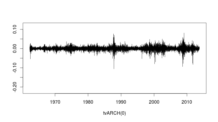
The pictures in Figure 1 show that the copula-based spectral methods developed in Dette et al., (2015) (where we refer to for details) indeed successfully account for serial features that remain out of reach in the traditional approach. The series considered in Figure 1 is the classical S&P500 index series, with $T=12092$ observations from 1962 through 2013; more precisely, that series contains the differences of logarithms of daily opening and closing prices for about 51 years. That series is generally accepted to be white noise, yielding perfectly flat periodograms. When rank-based copula periodograms are substituted for the classical ones, however, the picture looks quite different. Three rank-based copula periodograms are shown in Figure 1, for the quantile levels $0.1$, $0.5$ and $0.9$, respectively. The central one, corresponding to the central part of the marginal distribution, is compatible with the assumption of white noise. But the more extreme ones (associated with the quantile levels $0.1$ and $0.9$) yield a peak at the origin, pointing at a strong dependence in the tails which is definitely not present in the median part of the (marginal) distribution.

Figure 1: S&P500, 1962-2013: the smoothed rank-based copula periodograms for $\tau_{1}=\tau_{2}=0.1$, $0.5$ and $0.9$, respectively. All curves are plotted against $\omega/2\pi$.

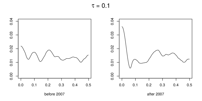
Now, all periodograms in Figure 1 were computed from the complete series (51 years, $1\leq t\leq 12092$), under the presumption of stationarity (more precisely, stationarity in distribution, for all $k$, of the couples $(X_{t},X_{t-k})$). Is that assumption likely to hold true? The wavelet-based test proposed by Nason, (2013) reveals significant changes in the behavior of that time series, with most significant changes taking place around 1975, 1997 and during the period 2007-2013. Moreover, two rank-based copula periodograms for $\tau_{1}=\tau_{2}=0.1$ computed before and after the year $2007$ are shown in Figure 2. We observe differences in the height of the peak at the origin before and after the year $2007$. These finding raise questions about the second limitation of traditional spectral methods, (second-order) stationarity. It has motivated the development of a rich strand of literature, mainly along four (largely overlapping) lines:

(a)

models with time-dependent parameters: inherently parametric, those models are mimicking the traditional ones, but with parameters varying over time—see Subba Rao, (1970) for a prototypical contribution, Azrak and Mélard, (2006) for an in-depth study of the time-varying ARMA case;

(b)

the evolutionary spectral methods, initiated by Priestley, (1965), where the process under study admits a spectral representation with time-varying transfer function—a second-order characterization, thus;

(c)

piecewise stationary processes, in relation with change-point analysis: see, e.g., Davis et al., (2005);

(d)

the locally stationary process approach initiated by Dahlhaus, (1997), based on the assumption that, over a short period of time (that is, locally in time), the process under study behaves approximately as a stationary one; related concepts have been developed recently by Dahlhaus and Subba Rao, (2006), Zhou and Wu, 2009a ; Zhou and Wu, 2009b , Roueff and Von Sachs, (2011) and Vogt, (2012); wavelet-based versions also have been considered, as in Nason et al., (2000). We refer to Dahlhaus (2012) for a survey of this approach.

Figure 2: S&P500: the smoothed rank-based copula periodograms for $\tau_{1}=\tau_{2}=0.1$ calculated for 512 days before and 512 day after 01.01.2007. Both curves are plotted against $\omega/2\pi.$

Those four approaches, as already mentioned, are not without overlaps: the original concept by Dahlhaus (1997) is based on time-varying (second-order) spectral representations, turned into time-domain linear MA($\infty$) ones by Dahlhaus and Polonik, (2006); Dahlhaus and Subba Rao, (2006) and Fryzlewicz et al., (2008) deal with locally stationary ARCH models; although much more general, Zhou and Wu, 2009a ; Zhou and Wu, 2009b also assume a form of time-varying nonlinear MA$(\infty)$ representation, and hence also resort to (a). Most references require moment assumptions, either by nature (being based on a spectral representation), or by the nature of the stationary approximation they are considering.

In this paper, we address the two limitations (i) and (ii) of traditional spectral analysis simultaneously by developing a locally stationary version of the quantile-related spectral analysis proposed in Dette et al., (2015). At the same time we provide a thorough theoretical underpinning for the proposed approach. While adopting the locally stationary ideas of (d), however, we turn them into a fully non-parametric and moment-free approach, adapted to the nature of quantile- and copula-based spectral concepts (see Harvey, (2010) for a related, time-domain, attempt). The definitions of local stationarity existing in the literature indeed are not general enough to accommodate quantile spectra, and we therefore formulate a new concept of local strict stationarity. Contrary to Dahlhaus and Polonik, (2006) and Zhou and Wu, 2009a ; Zhou and Wu, 2009b , who deal with time-varying (linear or nonlinear) moving averages, to Dahlhaus, (1997), which is based on time-varying second-order spectra, to Vogt, (2012), where the approximation is in terms of random variables and requires finite moments of order $\rho>0$, our approximation is directly based on joint distributions, and does not involve any moments nor specific data-generating processes. Its very general nature allows us to extend to the quantile context the definitions of a local spectrum, and to establish a central limit theorem for our local lag-window estimators.

The time-varying copula spectrum and its estimators are introduced in Section 2 and Section 3, respectively. In Section 4, we illustrate the application of the new methodology by means of a small simulation study and two real-life examples, while the theoretical properties of time-varying copula spectra and a corresponding lag-window estimator are investigated in Section 5. In particular, a central limit theorem for our local lag-window estimator is established. The proofs and additional information concerning the simulation studies and the datasets analyzed in Section 4.3 and 4.4 are deferred to an online supplement.

2 Local strict stationarity and local copula spectra

2.1 Locally strictly stationary processes

Consider a series $(X_{1},\ldots,X_{T})$ of length $T$ as being part of a triangular array $(X_{t,T},\ 1\leq t\leq T)$, $T\in\mathbb{N}$, of finite-length realizations of nonstationary processes $\{X_{t,T},\ t\in\mathbb{Z}\}$, $T\in\mathbb{N}$. The intuitive idea behind all definitions of local stationarity consists in the assumption that those processes have an approximately stationary behavior over a short period of time. More formally, one usually assume the existence of a collection, indexed by $\vartheta\in(0,1)$, of stationary processes $\{X^{\vartheta}_{t},\ t\in~{}\mathbb{Z}\}$ such that the nonstationary process $\{X_{t,T},\ t\in\mathbb{Z}\}$ can be approximated (in a suitable way), in the vicinity of time $t$, by the stationary process $\{X^{\vartheta}_{t},\ t\in~{}\!\mathbb{Z}\}$ associated with $\vartheta=t/T$.

The exact nature of this approximation has to be adapted to the specific problem under study. If the objective is a locally stationary extension of classical spectral analysis, only the autocovariances Cov$(X_{t,T},X_{s,T})$ have to be approximated. In the quantile-related context considered here, the joint distributions of $X_{t,T}$ and $X_{s,T}$ are the feature of interest, and traditional autocovariances are to be replaced with autocovariances of indicators, of the form Cov$(\mathbb{I}_{\{X_{t,T}\leq q_{t,T}(\tau_{1})\}},\mathbb{I}_{\{X_{s,T}\leq q_{s,T}(\tau_{2})\}})$, where $q_{t,T}(\tau_{1})$ and $q_{s,T}(\tau_{2})$ stand for the $\tau_{1}$-quantile of $X_{t,T}$ and the $\tau_{2}$-quantile of $X_{s,T}$, respectively, with $\tau_{1},\tau_{2}\in(0,1)$; see Li, (2008, 2012), Hagemann, (2013), or Dette et al., (2015). Such covariances only depend on the bivariate copulas of $X_{t,T}$ and $X_{s,T}$.

In a strictly stationary context, this leads to the so-called Laplace spectrum, first considered by Li, (2008) for a strictly stationary process $\{Y_{t},t\in\mathbb{Z}\}$ with marginal median zero. That spectrum is defined as

$$\mathcal{C}_{0.5,0.5}(\omega):=\frac{1}{2\pi}\sum_{k\in\mathbb{Z}}e^{-i\omega k}\text{Cov}(\mathbb{I}_{\{Y_{0}\leq 0\}},\mathbb{I}_{\{Y_{-k}\leq 0\}}),\qquad\omega\in(-\pi,\pi].$$

Li’s concept was extended by Hagemann, (2013), Li, (2012) and Dette et al., (2015) to general quantile levels. The most general version, which also takes into account cross-covariances of indicators, was introduced by Dette et al., (2015). Denoting by $q$ the marginal quantile function of $Y_{t}$, they define the copula spectral density kernel as

$$\mathcal{C}_{\tau_{1},\tau_{2}}(\omega):=\frac{1}{2\pi}\sum_{k\in\mathbb{Z}}e^{-i\omega k}\text{Cov}(\mathbb{I}_{\{Y_{0}\leq q(\tau_{1})\}},\mathbb{I}_{\{Y_{-k}\leq q(\tau_{2})\}}),\quad\tau_{1},\tau_{2}\in(0,1),\ \omega\in(-\pi,\pi].$$

Those definitions all heavily rely on the strict stationarity of the underlying time series; without this assumption, actually, they do not make much sense. It seems natural, thus, to look for some adequate notion of local stationarity that can be employed to characterize the notion of a local copula-based spectrum. However, the definitions of local stationarity previously considered in the literature are placing unnecessarily strong restrictions on the classes of processes that can be considered. In particular, Dahlhaus and Polonik, (2006), Dahlhaus and Subba Rao, (2006) and Vogt, (2012) rely on moment assumptions that are neither desirable nor natural in a quantile context, and are not required for the definition of copula spectra. We therefore introduce a new concept of local strict stationarity which completely avoids moment assumptions. That concept is not totally unrelated to the existing ones, though, and we also show that, under adequate conditions, processes that fit into the framework of Dahlhaus and Subba Rao, (2006) or Dahlhaus and Polonik, (2006) are locally strictly stationary in the new sense; see Section 5.1 for details. Similar results certainly also could be obtained for the Zhou and Wu, 2009a ; Zhou and Wu, 2009b concept, but they are less obvious and, in order to not overload the paper, we do not pursue into that direction.

The copula spectral density kernels of a stationary process $\{Y_{t}\}$ are defined in terms of its bivariate marginal distribution functions. Therefore, it is natural to use bivariate marginal distribution functions when evaluating, in the definition of local stationarity, the distance between the non-stationary process $\{X_{t,T}\}$ and its stationary approximation $\{X^{\vartheta}_{t}\}$.

Definition 2.1.

A triangular array $\{(X_{t,T})_{t\in\mathbb{Z}}\}_{T\in\mathbb{N}}$ of processes is called locally strictly stationary (of order two) if there exists a constant $L>0$ and, for every $\vartheta\in(0,1)$, a strictly stationary process $\{X^{\vartheta}_{t},t\in\mathbb{Z}\}$ such that, for every $1\leq r,s\leq T,$

$$\big{\|}F_{r,s;T}(\cdot,\cdot)-G^{\vartheta}_{r-s}(\cdot,\cdot)\big{\|}_{\infty}\leq L\Big{(}\max(|r/T-\vartheta|,|s/T-\vartheta|)+{1}/{T}\Big{)},$$ (2.1)

where $\|\cdot\|_{\infty}$ stands for the supremum norm, while $F_{r,s;T}(\cdot,\cdot)$ and $G^{\vartheta}_{k}(\cdot,\cdot)$ denote the joint distribution functions of $(X_{r,T},X_{s,T})$ and $(X^{\vartheta}_{0},X^{\vartheta}_{-k})$, respectively.

Here, ‘of order two’ refers to the fact that (2.1) is based on bivariate distributions only. Letting $y$ tend to infinity in $F_{r,s;T}(x,y)$ and $G^{\vartheta}_{k}(x,y)$, we get an analogous condition for the marginal distributions $F_{t;T}$ and $G^{\vartheta}$ of $X_{t,T}$ and $X^{\vartheta}_{0}$, namely

$$\big{\|}F_{t;T}(\cdot)-G^{\vartheta}(\cdot)\big{\|}_{\infty}\leq L\big{|}t/T-\vartheta\big{|}+L/{T}.$$ (2.2)

Intuitively, (2.1) and (2.2) imply that the univariate and bivariate distribution functions $F_{t;T}$ and $F_{r,s;T}$ of the process $\{X_{t,T}\}$ are allowed to change smoothly over time. A crucial advantage of this definition is its nonparametric nature, as it does not depend on any specific data-generating mechanism.

Whenever the data-generating process can be described in terms of a parametric model, strict stationarity in the sense of Definition 2.1 holds if the underlying parameters change smoothly over time. Familiar examples include MA$(\infty)$, ARCH$(\infty)$ and GARCH$(p,q)$ models with time-varying coefficients. Sufficient conditions for local strict stationarity of those models are discussed in Section 5.1, where we also provide explicit forms of the strictly stationary approximating processes.

2.2 Local copula spectral density kernels

Turning to the definition of a localized version of copula spectral density kernels, first consider the copula cross-covariance kernels associated with the strictly stationary process $\{X^{\vartheta}_{t},t\in~{}\mathbb{Z}\}$, $\vartheta\in(0,1)$. The lag-$h$-copula cross-covariance kernel of $\{X^{\vartheta}_{t}\}$, as defined in Dette et al., (2015), is

$$\gamma^{\vartheta}_{h}(\tau_{1},\tau_{2}):=\mathrm{Cov}(\mathbb{I}_{\{X^{\vartheta}_{t}{}\leq q^{\vartheta}(\tau_{1})\}},\mathbb{I}_{\{X^{\vartheta}_{t-h}{}\leq q^{\vartheta}(\tau_{2})\}}),\quad\tau_{1},\tau_{2}\in(0,1),$$

where $q^{\vartheta}(\tau)$ denotes $X^{\vartheta}_{t}$’s marginal quantile of order $\tau$.

The cross-covariances involved in the above definition always exist, and their collection (for $\tau_{1},\tau_{2}\in(0,1)$ and given lag $h$) provides a canonical characterization of the joint copula of $(X^{\vartheta}_{t}{},X^{\vartheta}_{t-h}{})$, hence, an approximate (in the sense of (2.1)) description of the joint copula of all couples of the form $(X_{t,T},X_{t-h,T})$. Therefore we also call $\gamma^{\vartheta}_{h}(\tau_{1},\tau_{2})$ the time-varying lag-$h$-copula cross-covariance kernel of $\{X_{t,T}\}.$ If we assume that, for all $\tau_{1},\tau_{2}\in(0,1)$, the lag-$h$-covariance kernels $\gamma^{\vartheta}_{h}(\tau_{1},\tau_{2})$ are absolutely summable, we moreover can define the local or time-varying copula spectral density kernel of $\{X_{t,T}\}$ as

$$\mathfrak{f}^{\vartheta}(\omega,\tau_{1},\tau_{2}):=\frac{1}{2\pi}\sum_{h=-\infty}^{\infty}\gamma^{\vartheta}_{h}(\tau_{1},\tau_{2})e^{-ih\omega},\ \ \tau_{1},\tau_{2}\in(0,1),\ \ \omega\in(-\pi,\pi].$$ (2.3)

The time-varying cross-covariance kernel then admits the representation

$$\gamma^{\vartheta}_{h}(\tau_{1},\tau_{2})=\int_{-\pi}^{\pi}e^{ih\omega}\mathfrak{f}^{\vartheta}(\omega,\tau_{1},\tau_{2})d\omega,\qquad\omega\in(-\pi,\pi],\quad\tau_{1},\tau_{2}\in(0,1).$$

Comparing those representations with the local spectral densities of Dahlhaus (1997), we see that the autocovariances of the approximating processes there are replaced by copulas. This indicates that the local spectral density kernels (2.3) can be viewed as a completely non-parametric generalization of classical $L^{2}$-based tools. In particular, those kernels can capture pairwise serial dependencies of arbitrary forms. For more detailed comparisons, we refer to Dette et al., (2015) and Kley et al., (2016). The usefulness of the concepts discussed here for data analysis is provided, via simulation and the analysis of two real datasets, the classial S$\&$P 500 and a meteorological one, in Section 4.

3 Estimation of local copula spectra

Given observations $X_{1,T},\dots,X_{T,T}$, the classical approach to the estimation of the time-varying spectral density of a locally stationary time series consists in considering a subset of $n$ data points centered around a time point $t_{0}.$

To formalize ideas, let $m_{T}$ be a sequence of positive integers diverging to infinity as $T\to~{}\!\infty$, and define the discrete neighborhood $\mathcal{N}_{t_{0},T}:=\{1\leq t\leq T:|t_{0}-t|<m_{T}\},$ with cardinality $n=n(m_{T},T)$. Denoting by $\omega_{j,n}=2\pi j/n,1\leq j\leq\lfloor\frac{n+1}{2}\rfloor$ the positive Fourier frequencies, let $\varphi_{n}:\omega\mapsto\varphi_{n}(\omega):=\omega_{j,n}$ be the piecewise constant function mapping $\omega\in(0,\pi)$ to the closest Fourier frequency, i.e. to the frequency $\omega_{j,n}$ such that $\omega\in(\omega_{j,n}-\frac{2\pi}{n},\,\omega_{j,n}+\frac{2\pi}{n}]$. Defining

$$T(k):=\{t\in\mathcal{N}_{t_{0},T}:t+k\in\mathcal{N}_{t_{0},T}\},\quad\tilde{F}_{t_{0};T}(x):=\frac{1}{2T^{4/5}}\sum_{|t-t_{0}|\leq T^{4/5}}\mathbb{I}_{\{X_{t,T}\leq x\}},$$

and $\hat{q}_{t_{0},T}(\tau):=\tilde{F}_{t_{0};T}^{-1}(\tau)$, consider the local lag-window estimator (at the Fourier frequen-cies $\omega_{j,n}=2\pi j/n$)

$$\hat{\mathfrak{f}}_{t_{0},T}(\omega_{j,n},\tau_{1},\tau_{2}) := \frac{1}{2\pi}\sum_{|k|\leq n-1}K(k/B_{n})e^{-i\omega_{j,n}k}$$ (3.1)

$$\quad\times\ \frac{1}{n}\sum_{t\in T(k)}\Big{(}\mathbb{I}_{\{X_{t,T}\leq\hat{q}_{t_{0},T}(\tau_{1})\}}-\tau_{1}\Big{)}\Big{(}\mathbb{I}_{\{X_{t+k;T}\leq\hat{q}_{t_{0},T}(\tau_{2})\}}-\tau_{2}\Big{)},$$

where $B_{n}\rightarrow\infty$ as $n\rightarrow\infty$ and $K:\mathbb{R}\to\mathbb{R}$ is continuous in $x=0$ and satisfies $K(0)=1$ and $\lim_{|x|\to\infty}K(x)=0$. In order to extend this estimator $\hat{f}_{t_{0},T}(\cdot,\tau_{1},\tau_{2})$ to the interval $(0,\pi),$ let $\hat{f}_{t_{0},T}(\omega,\tau_{1},\tau_{2}):=\hat{f}_{t_{0},T}(\varphi_{n}(\omega),\tau_{1},\tau_{2}).$ In Section 5.2 below, we prove that, under mild conditions on the bandwidth parameters and the underlying time series, the local lag-window estimator is consistent for the copula spectral density $\mathfrak{f}^{\vartheta}(\omega,\tau_{1},\tau_{2})$ and asymptotically normally distributed. This is a novel result even in the stationary case, as Kley et al., (2016) consider an estimator based on smoothed periodograms instead.

Before we address the asymptotic theory for the new estimators, we illustrate their properties and advantages by means of a brief simulation study and a detailed analysis of two real-life datasets.

4 Simulations and an empirical study

One important practical aspect of the estimation of a quantile spectral density is the choice of a local window length $n$ and a smoothing parameter $B_{n}$. In Section 5.2 and Theorem 5.1, we derive the asymptotic distribution of the estimator, which allows to derive an expression for the smoothing parameters that minimizes the asymptotic mean squared error (see Remark 5.3 for additional details). Those expressions, of course, cannot be readily used in practice, since they depend on the actual time-varying copula spectral densities and their derivatives, which are unknown. Estimating such derivatives is even more difficult than estimating the original spectral density, and a plug-in approach to bandwidth selection therefore seems difficult to implement. For the estimation of local $L^{2}$-spectra, an interesting alternative has been proposed by Cranstoun et al., (2002). Unfortunately, that approach relies on wavelets instead of local windows for localization in time; whether it can be implemented here is not clear. For the implementation of our methodology, we propose to study different local window lengths and bandwidth parameters and in the simulation study we illustrate the performance of the estimators for different window lengths.

4.1 Heatmaps: calibrating the color scale

Plots of time-varying spectral densities and their estimators are provided in the form of time-frequency heatmaps. The vertical axis in all those plots represents frequencies ($\omega/2\pi$, ranging from 0 to 0.5), the horizontal axis the span of time $1,\ldots,T$ over which the time-varying spectral quantities are estimated. All $3\times 3$ figures in this section show the real and imaginary parts for different combinations of quantile orders, organized as shown in Table 1.

$\mathfrak{\hat{f}}_{t_{0},T}({\omega,\alpha,\alpha})$	${\Im\mathfrak{\hat{f}}_{t_{0},T}({\omega,\beta,\alpha})}$	${\Im\mathfrak{\hat{f}}_{t_{0},T}({\omega,\gamma,\alpha})}$
${\Re\mathfrak{\hat{f}}_{t_{0},T}({\omega,\beta,\alpha})}$	${\mathfrak{\hat{f}}_{t_{0},T}({\omega,\beta,\beta})}$	${\Im\mathfrak{\hat{f}}_{t_{0},T}({\omega,\gamma,\beta})}$
${\Re\mathfrak{\hat{f}}_{t_{0},T}({\omega,\gamma,\alpha})}$	${\Re\mathfrak{\hat{f}}_{t_{0},T}({\omega,\gamma,\beta})}$	${\mathfrak{\hat{f}}_{t_{0},T}({\omega,\gamma,\gamma})}$

Table 1: Patterns for the $3\times 3$ time-frequency heatmaps in Figures 5-8 and 11; throughout, we use $\alpha=0.1$, $\beta=0.5$ and $\gamma=0.9,$ with $t_{0}\in{\cal T}_{0}\subset\{1,\dots,T\}$ and $\omega\in(0,\pi)$. For example, the top-right corner, in all those figures, displays a time-frequency plot of the imaginary parts of the collection $\big{(}\mathfrak{\hat{f}}_{t_{0},T}(\omega,0.9,0.1)\big{)}_{t_{0}\in{\cal T}_{0},\omega\in\Omega}$.

The spectral values themselves (for $\tau_{1}=\tau_{2}=\tau$), or their real and imaginary parts (for $\tau_{1}\neq\tau_{2}$) are represented via a continuous $(\tau_{1},\tau_{2})$-dependent color code, ranging from cyan and light blue (for small values) to dark blue, yellow, orange, and red (for large values). As explained below, this color code also has an interpretation in terms of significance of certain $p$-values. This latter interpretation requires a preliminary calibration step, though. Indeed, being ‘small’, for a $(\tau_{1}=\tau_{2}=\tau)-$periodogram value (which by nature is nonnegative real) does not have the same meaning as being ‘small’ for the imaginary or the real part of some $(\tau_{1}^{\prime},\tau_{2}^{\prime})-$cross-periodogram (for which negative values are possible): in order to make inter-frequency comparisons possible, a meaningful color code therefore has to be $(\tau_{1},\tau_{2})$-specific. For this purpose we introduce a distribution-free simulation-based calibration that fully exploits the properties of copula-based quantities.

To explain the idea behind this calibration step, consider plotting, for some subset ${\cal T}_{0}\times\Omega$ (with ${\cal T}_{0}\subset\{1,...,T\}$ and $\Omega\subset(0,\pi)$), a collection $\big{(}\Re\mathfrak{\hat{f}}_{t_{0},T}(\omega,\tau_{1},\tau_{2})\big{)}_{t_{0}\in{\cal T}_{0},\omega\in\Omega}$ of the real parts (the imaginary parts are dealt with exactly the same way) of estimators computed from the realization $X_{1},....,X_{T}$ of some time series of interest. Assume that a bandwidth $B_{n}$ and a window length $n$ are used for the estimation. A color is then assigned to each value of $\Re\mathfrak{\hat{f}}_{t_{0},T}(\omega,\tau_{1},\tau_{2})$ along the following steps:

(i)

simulate $M=10^{4}$ independent realizations $(U_{1,m},\ldots,U_{n,m})$, $m=1,...,M$ of an i.i.d. sequence of random variables of length $n$ (uniform over $[0,1]$, for instance – but, our method being distribution-free, this is not required);

(ii)

for each of those $M$ realizations, compute the estimator $\mathfrak{\hat{f}}_{t_{0},T}^{U,m}(\omega,\tau_{1},\tau_{2})$ of the local spectral density based on the same bandwidth $B_{n}$; note that the number $n$ of observations in each replication equals the window length used for our original collection;

(iii)

define, for each $m=1,...,M=10^{4}$, the quantities $Q_{\max}^{m}(\tau_{1},\tau_{2}):=\max_{\omega}\Re\mathfrak{\hat{f}}_{t_{0},T}^{U,m}(\omega,\tau_{1},\tau_{2})$ and $Q_{\min}^{m}(\tau_{1},\tau_{2}):=\min_{\omega}\Re\mathfrak{\hat{f}}_{t_{0},T}(\omega,\tau_{1},\tau_{2})$; obtain the empirical $99.5\%$ quantile $q_{\max}(\tau_{1},\tau_{2})$ of $(Q_{\max}^{m}(\tau_{1},\tau_{2}))_{m=1,...,M}$, and the empirical $0.5\%$ quantile $q_{\min}(\tau_{1},\tau_{2})$ of $(Q_{\min}^{m}(\tau_{1},\tau_{2}))_{m=1,...,M}$, respectively.

The color palette then is set as follows: all points $(t_{0},\omega)\in{\cal T}_{0}\times\Omega$ with $\Re\mathfrak{\hat{f}}_{t_{0},T}(\omega,\tau_{1},\tau_{2})$ value in $[q_{\min}(\tau_{1},\tau_{2}),q_{\max}(\tau_{1},\tau_{2})]$ receive dark blue color. Next, letting

$$v_{\min}(\tau_{1},\tau_{2}) :=\min(\min_{t_{0},\omega}\Re\mathfrak{\hat{f}}_{t_{0},T}(\omega,\tau_{1},\tau_{2}),q_{\min}(\tau_{1},\tau_{2})-(q_{\max}(\tau_{1},\tau_{2})-q_{\min}(\tau_{1},\tau_{2}))),$$

$$v_{\max}(\tau_{1},\tau_{2}) :=\max(\max_{t_{0},\omega}\Re\mathfrak{\hat{f}}_{t_{0},T}(\omega,\tau_{1},\tau_{2}),q_{\max}(\tau_{1},\tau_{2})+(q_{\max}(\tau_{1},\tau_{2})-q_{\min}(\tau_{1},\tau_{2}))),$$

all points $(t_{0},\omega)$ for which $\Re\mathfrak{\hat{f}}_{t_{0},T}(\omega,\tau_{1},\tau_{2})$ lies in the interval $[v_{\min}(\tau_{1},\tau_{2}),q_{\min}(\tau_{1},\tau_{2})]$ receive a color ranging, according to a linear scale, from cyan to light and dark blue, while the colors for the interval $[q_{\max}(\tau_{1},\tau_{2}),v_{\max}(\tau_{1},\tau_{2})]$ similarly range from dark blue to yellow and red.

All our time-frequency heat diagrams thus have the following interpretation. For each given choice of $(\tau_{1},\tau_{2})$ and a timepoint $t_{0}$, the probability, under the hypothesis of (strong) white noise, that the real (resp., the imaginary) part at time $t=t_{0}$ of the smoothed $(\tau_{1},\tau_{2})$-time-varying periodogram lies entirely in the dark blue area is approximately $0.01.$ Hence, the presence of light blue, cyan or orange-red zones in a diagram indicates a significant (at probability level $1\%$) deviation from white noise behavior. The location of those zones moreover tells us where in the spectrum, and when in the period of observation, those significant deviations take place, along with an evaluation of their magnitude. The correspondence between the actual size of the estimate and the colors used is provided by the color scale on the right-hand side of each diagram. Note that here and in the sequel, we use the terminology ’white noise’ to denote i.i.d. (and not just uncorrelated) variables.

This calibration method yields a universal distribution-free and model-free color scaling which also provides (as far as dark blue regions are concerned) a hypothesis testing interpretation of the results. The same color code is used for the empirical analyses in Sections 4.3 and 4.4, as well as for the simulations in Section 4.2. Currently, an R-package containing the codes used here is in preparation (a preliminary version is available upon request).

4.2 Simulations

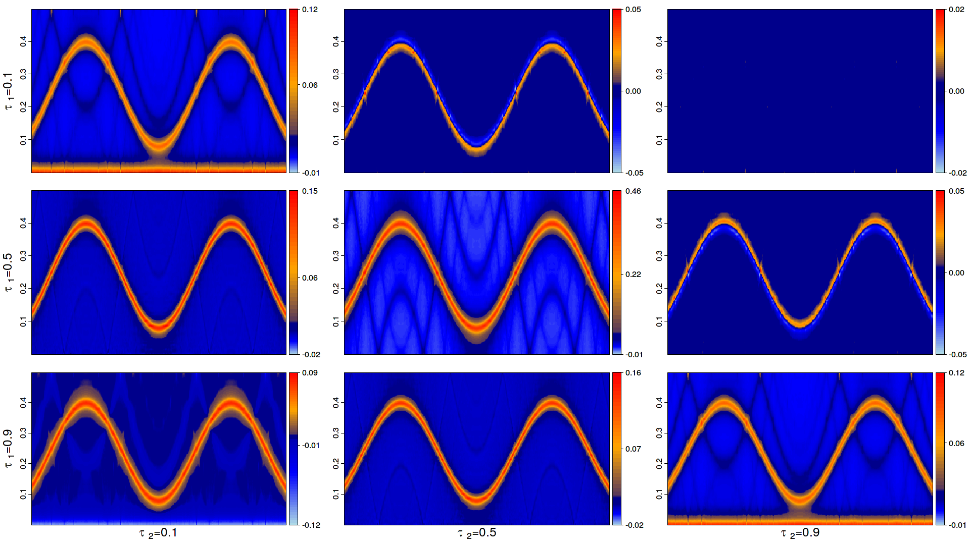
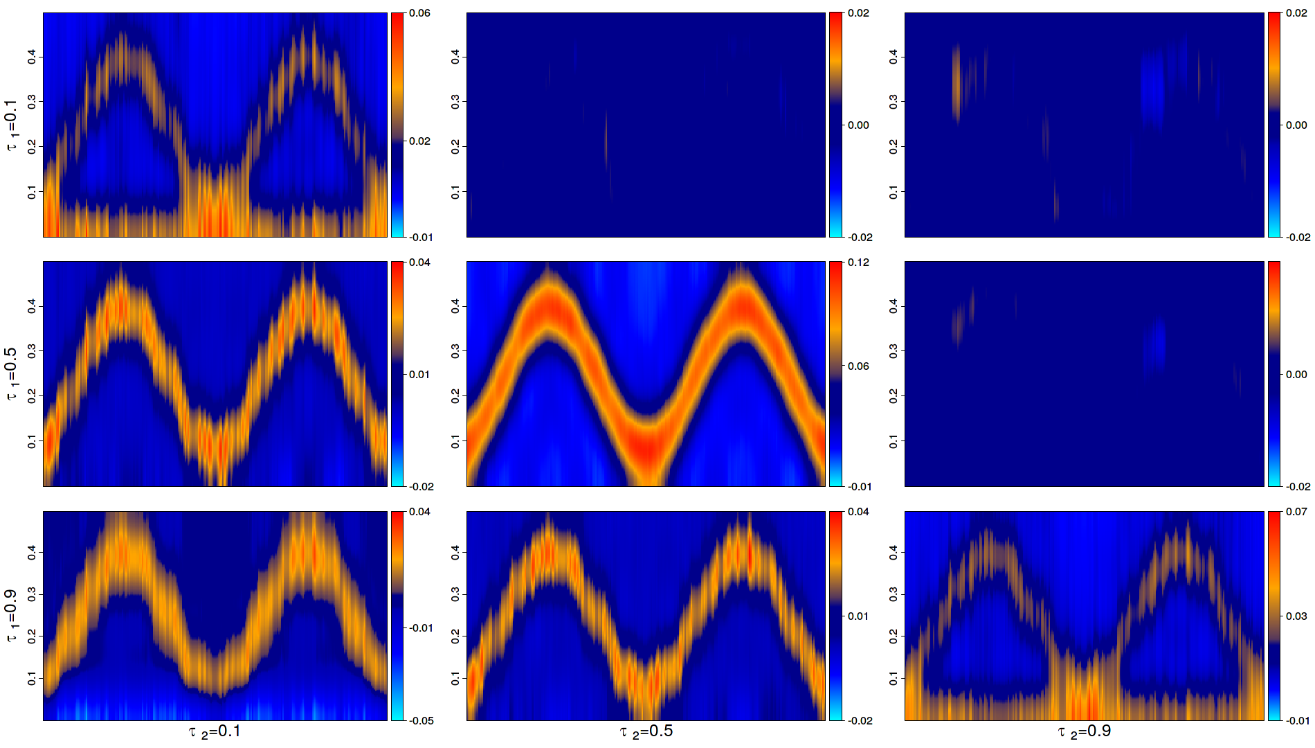
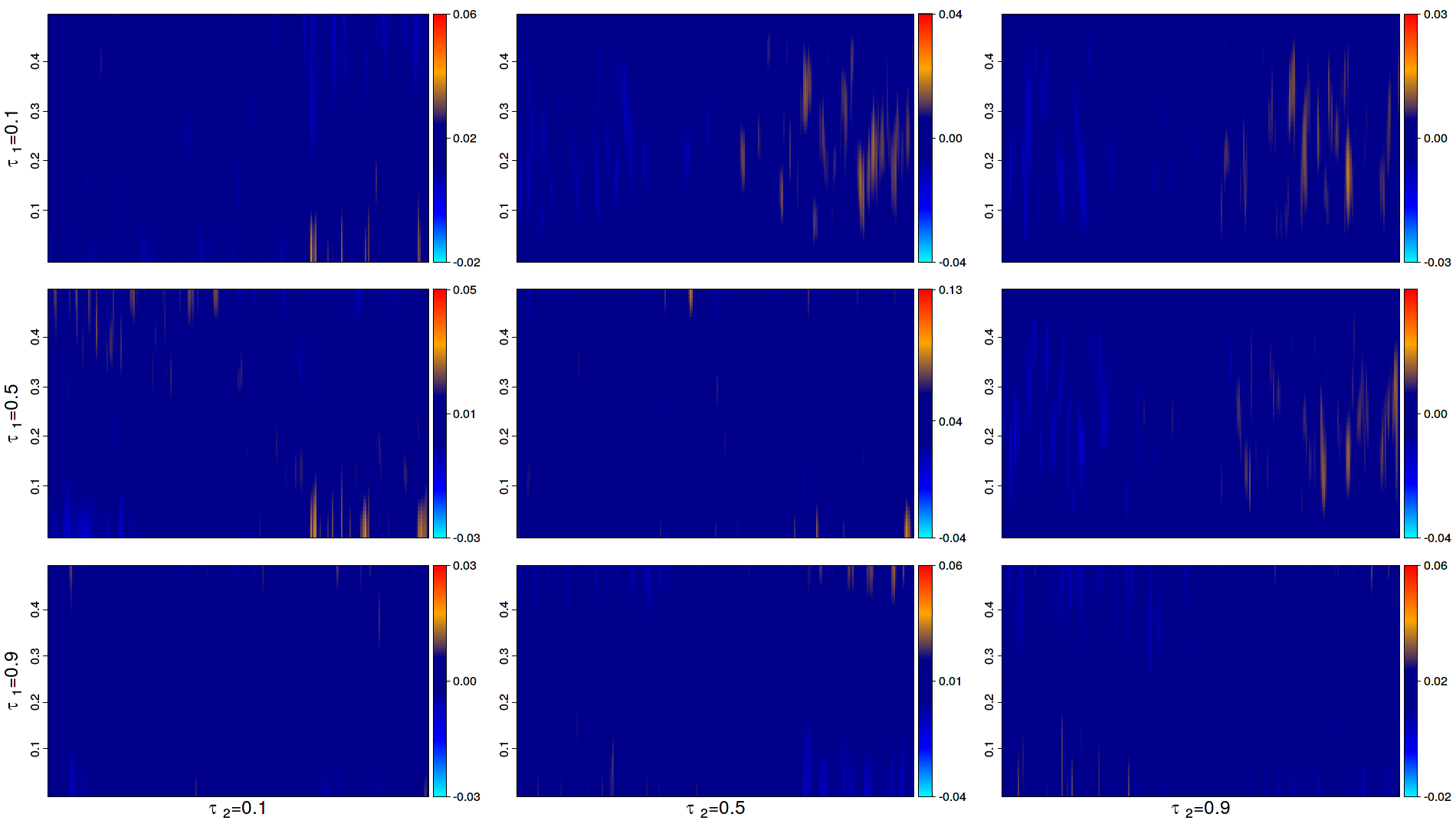
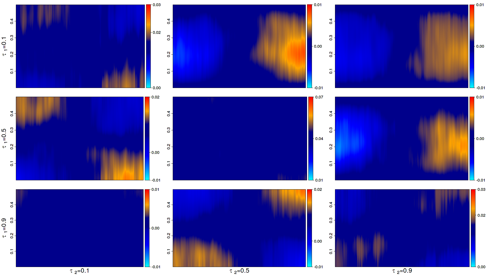
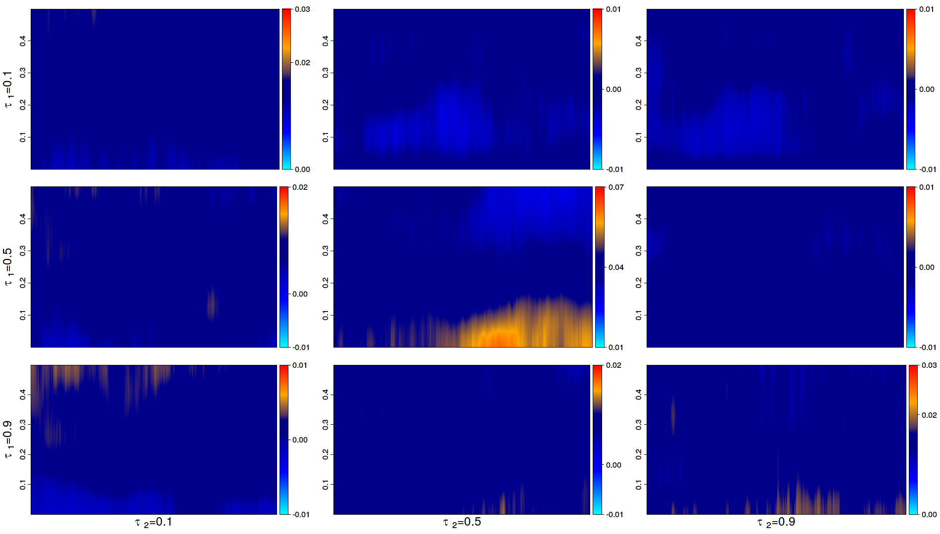
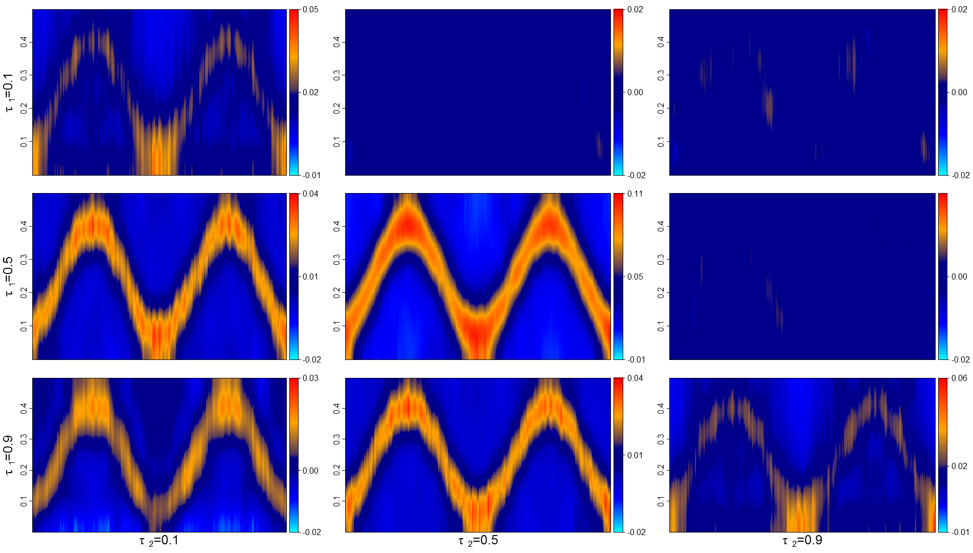
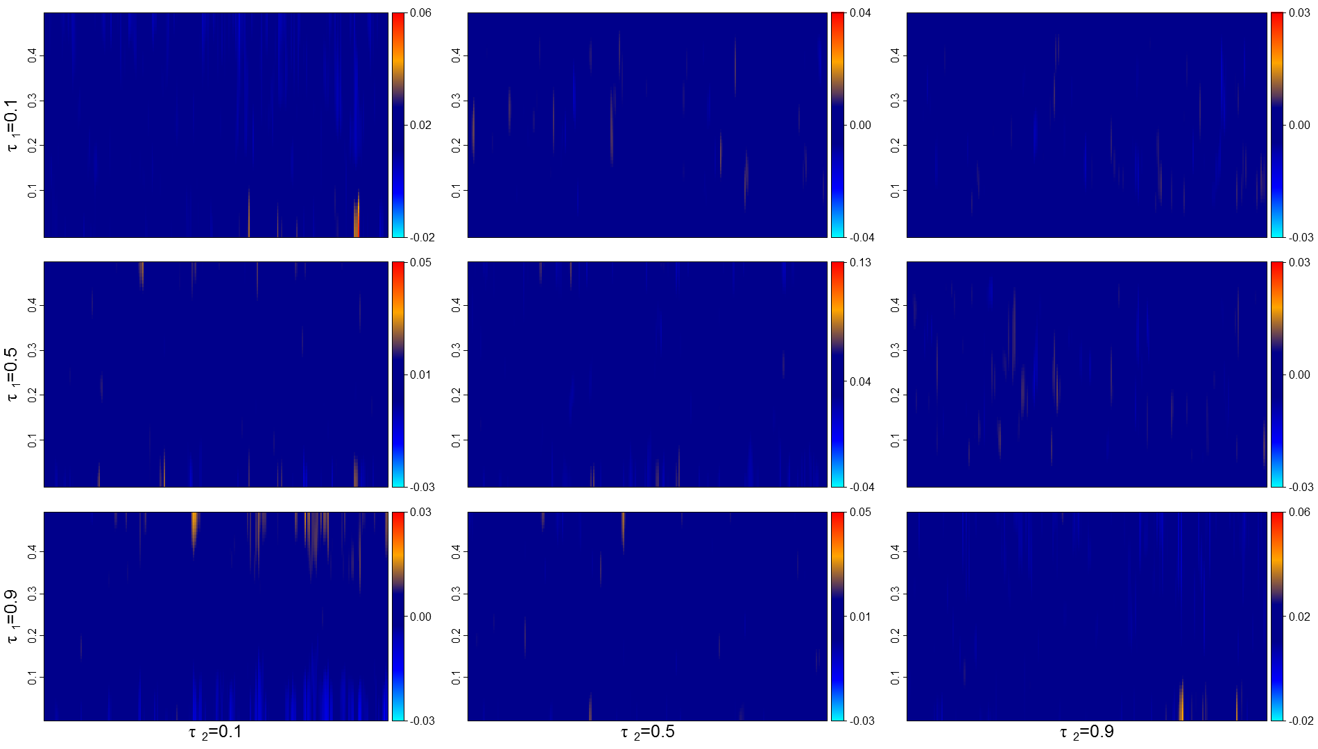
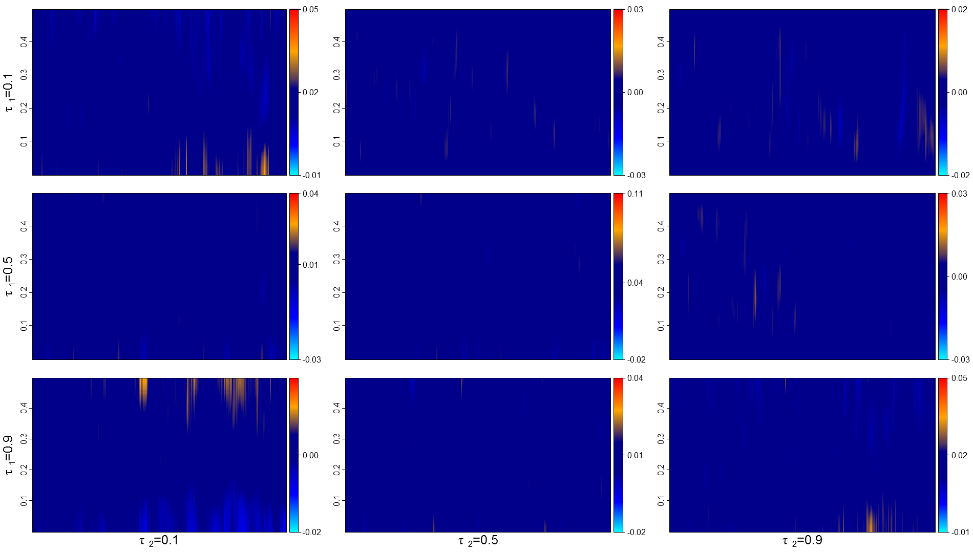
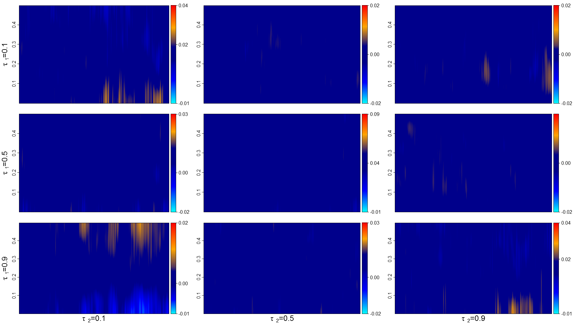
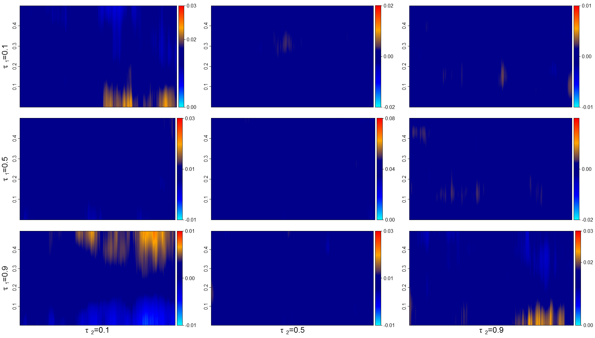
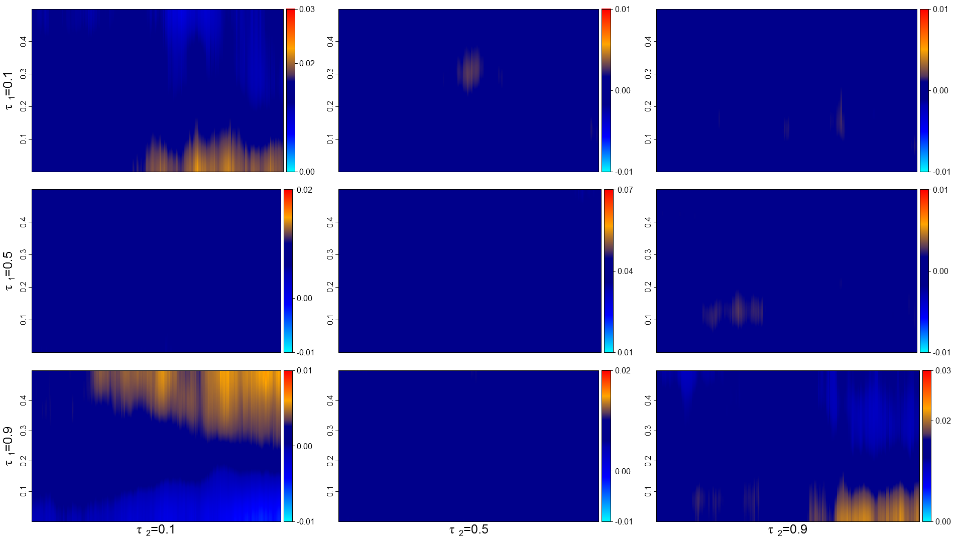
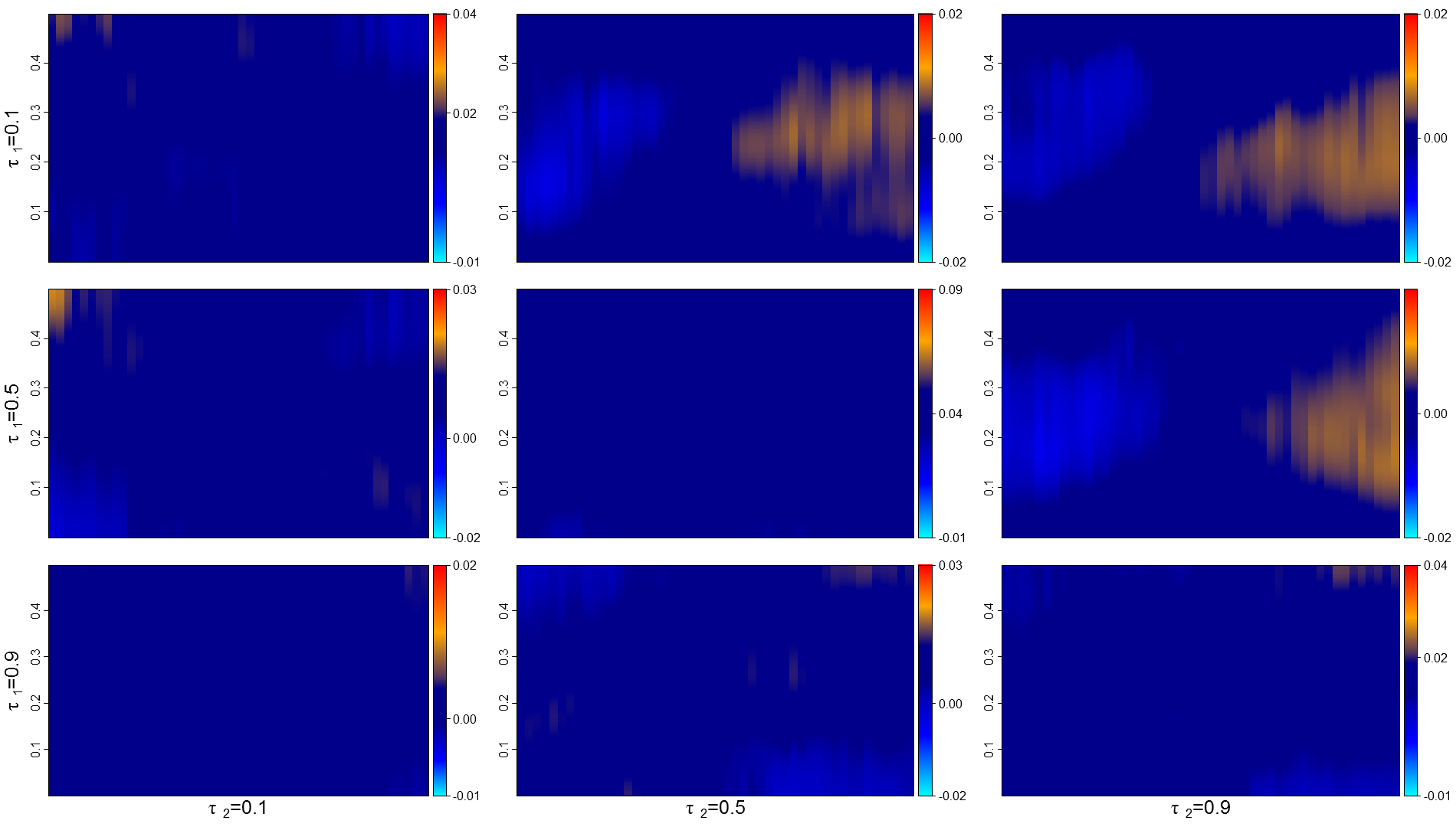
This section provides a numerical illustration of the performance of the new estimators of the time-varying copula spectral densities in two time-varying models that have been considered elsewhere in the literature. For both models, six time-frequency heat plots, labeled (a)-(f), of time-varying copula spectral densities are provided, for each combination of the quantile levels $0.1$, $0.5$, and $0.9$, using the color code described in Section 4.1:

(a)

the actual time-varying copula spectral densities and

(b)-(f)

the local lag-window estimators of the copula spectral densities for different window length $n.$

Currently, we do not have simple closed-form expressions for the actual spectra, and we doubt such expressions are possible (but for the theoretical definition (2.3)). This is in contrast with classical $L^{2}$ spectral analysis where, at least for linear processes, explicit representation for the spectra are readily available. Such lack of simple analytic expressions is not surprising since, even for linear processes, the impact of the linear representation coefficients on joint distributions (as opposed to covariances) is bound to be quite complicated, and crucially depends on innovation densities. From a practical point of view, this is not a major drawback, though, as for any given linear representation very good approximations of the copula spectra can be obtained within a few minutes via simulations. The actual copula spectral densities in (a) were obtained by simulating, for each $t_{0}$ in ${\cal T}_{0}$, $R=1000$ independent replications, all of length $2^{11}$, of the strictly stationary approximation $(X^{t_{0}/T}_{t})_{t=1,...,2^{11}}$, computing the corresponding lag-window estimators $\hat{\mathfrak{f}}^{r}_{t_{0},T}(\omega,\tau_{1},\tau_{2})$, say, for $r=1,...,R$, and averaging them (over $r=1,...,R$) for each fixed $(t_{0},\omega)\in{\cal T}_{0}\times\Omega$.

The estimators in (b)-(f) are computed from one realization, of length $T=2^{13}$, of the (nonstationary) process under consideration with a bandwidth $B_{n}=10$ and local window lengths $n=128,256,512,1024,2048$. Additional examples with time series of length $T=2^{11},2^{12}$ are available in Section A.2.3 of the online appendix. Our findings indicate that, for shorter time-series lengths, estimating ‘fastly changing’ dependence structures may become difficult. If the changes are very smooth, as in the QAR example of Section 4.2.2, the results for short time series are still reasonable. For $K$, we used the Parzen window

$$K(u)=(1-6u^{2}+6|u|^{3})\mathbb{I}_{\{|u|\leq 0.5\}}+2(1-|u|)^{3}\mathbb{I}_{\{0.5\leq|u|\leq 1\}}.$$

In each case, the sets ${\cal T}_{0}$ and $\Omega$ were chosen as ${\cal T}_{0}:=\{32k|k=\lceil n/2\rceil,\dots,\lfloor T-n/2\rfloor\}$ and $\Omega:=\{2\pi j/n|j=1,...,(n-2)/2\}.$

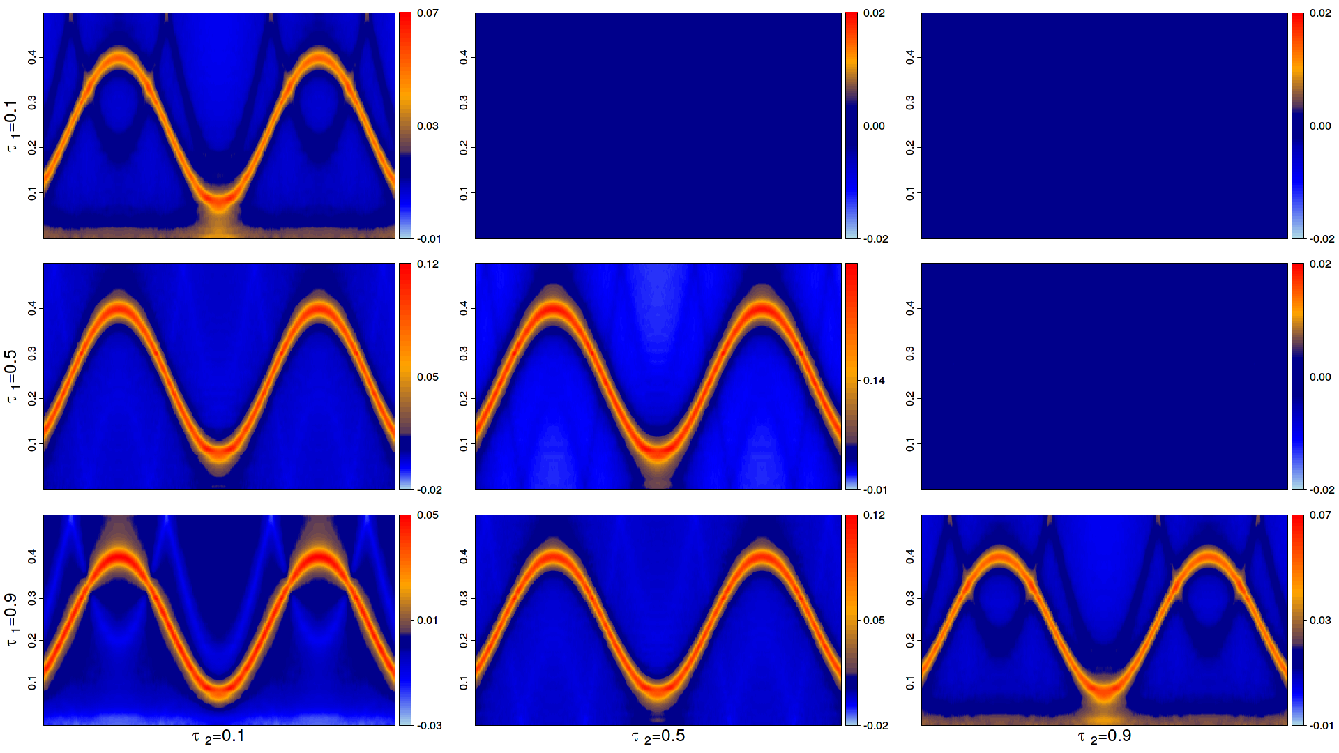
4.2.1 Cauchy tvAR(2)

In Figure 3, we display heatmapss for a time-varying AR(2) process with equation

$$X_{t,T}=1.8\cos(1.5-\cos(2\pi t/T))X_{t-1,T}-0.81X_{t-2,T}+Z_{t}\vspace{-1mm}$$ (4.1)

and i.i.d. noise $Z_{t}$ with Cauchy distribution. Its strictly stationary approximation at $t_{0}=\vartheta T$, for $0\leq\vartheta\leq 1$, is

$$X_{t}^{\vartheta}=1.8\cos(1.5-\cos(2\pi\vartheta))X_{t-1}^{\vartheta}-0.81X_{t-2}^{\vartheta}+\zeta_{t}\vspace{-1mm}$$ (4.2)

where the $\zeta_{t}$’s are i.i.d. noise  with the same Cauchy density as the $Z_{t}$’s.

The form of the equation is taken from Dahlhaus, (2012), where we replaced the Gaussian innovations with Cauchy ones, thus violating the moment assumptions of classical spectral analysis. The resulting process exhibits a time-varying periodicity which is clearly visible in the heat diagrams associated with the real parts of its time-varying copula spectral densities, displayed in the lower triangular parts of Figures 3(a)-(f). The imaginary parts of the spectra are shown in the upper triangular parts of the same figures; note that, due to time-irreversibility (see Hallin et al. 1988), those imaginary parts exhibit significant yellow regions in the actual spectral density (a). The peaks are, however, very narrow, thus quite difficult to estimate, and essentially disappear in the estimated versions (b)-(f). The proposed lag-window estimator nevertheless is able to recover the structure of the spectral densities over a broad range of window lengths.

Also note the significant peak around zero appearing in the diagrams associated with extreme quantiles ($\tau_{1},\tau_{2}=0.1$ and $0.9$), indicating persistence in tail events—a phenomenon that totally escapes traditional analyses. The change over time is rather fast and therefore the influence of the window length on the estimator is clearly visible. A very short window length, like $n=128$ in $(b),$ makes it very difficult to reconstruct the copula spectral densities for the extreme quantiles $(\tau=(0.1,0.1)\text{ or }\tau=(0.9,0.9))$ still the periodic peak remains quite significant, while a much larger one ($n=2048$ in (f)) one. leads to a loss of details. The estimators remain stable, though, over a broad range of window lengths ($n=256-1024$).

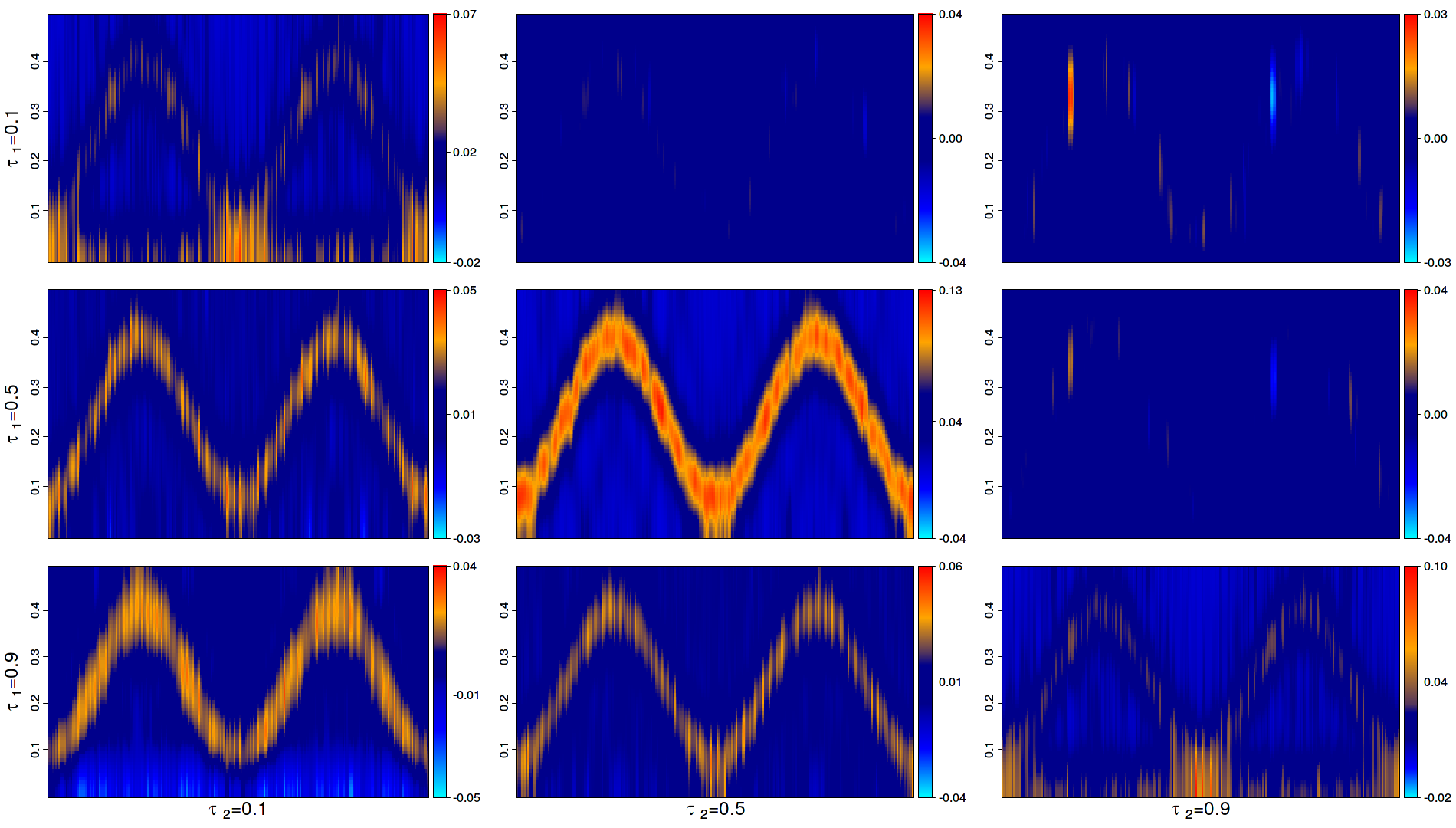
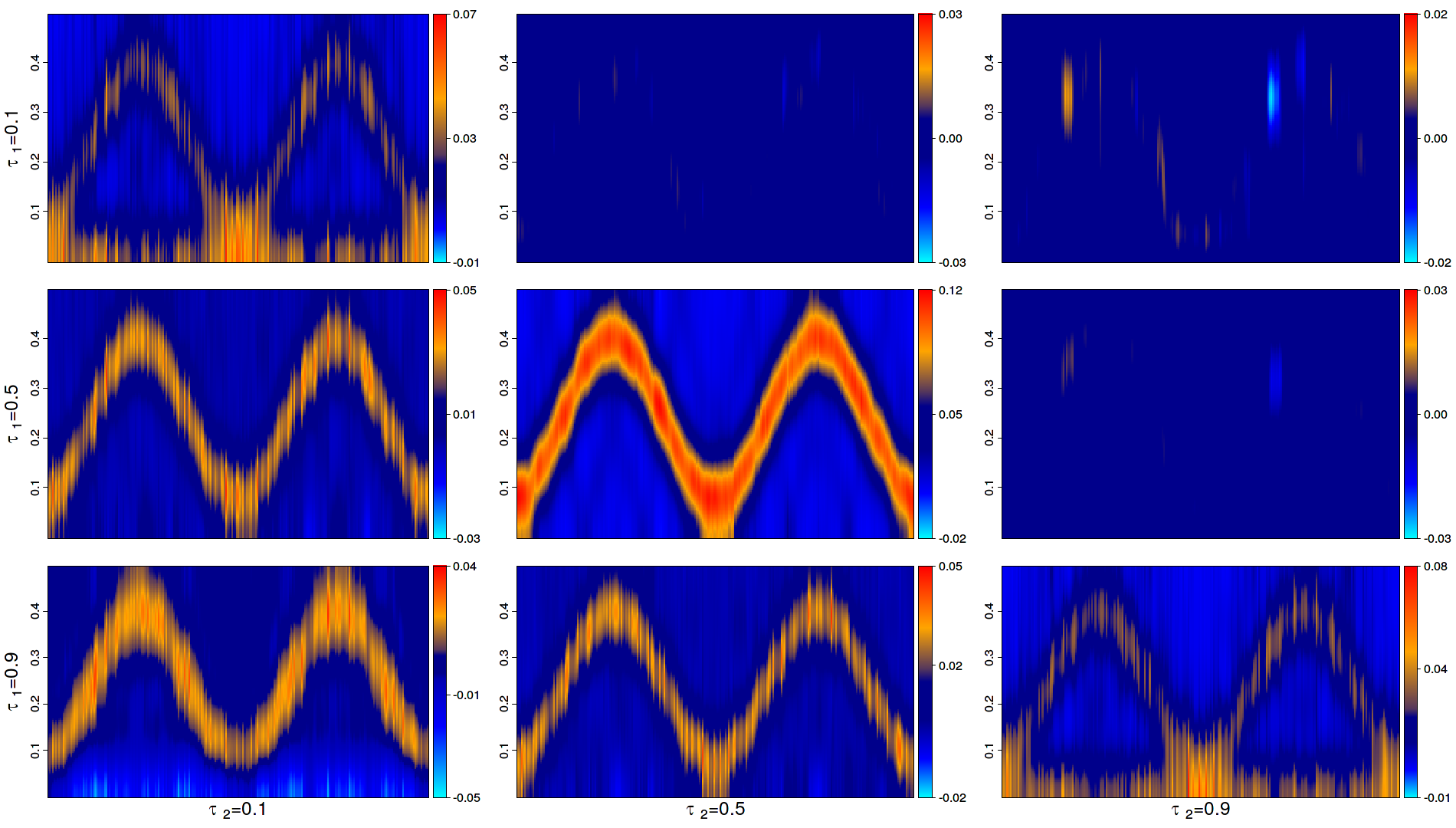
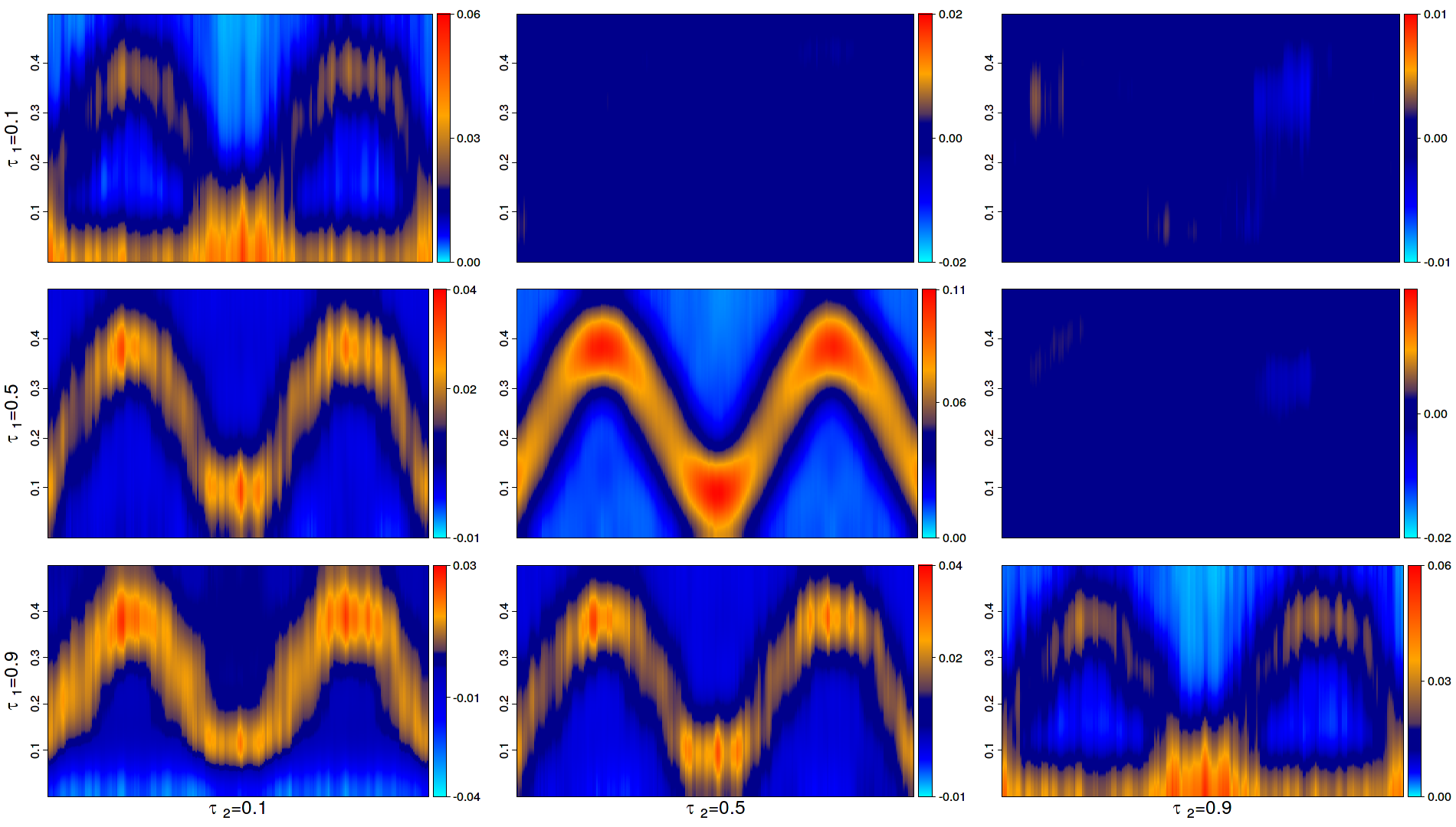
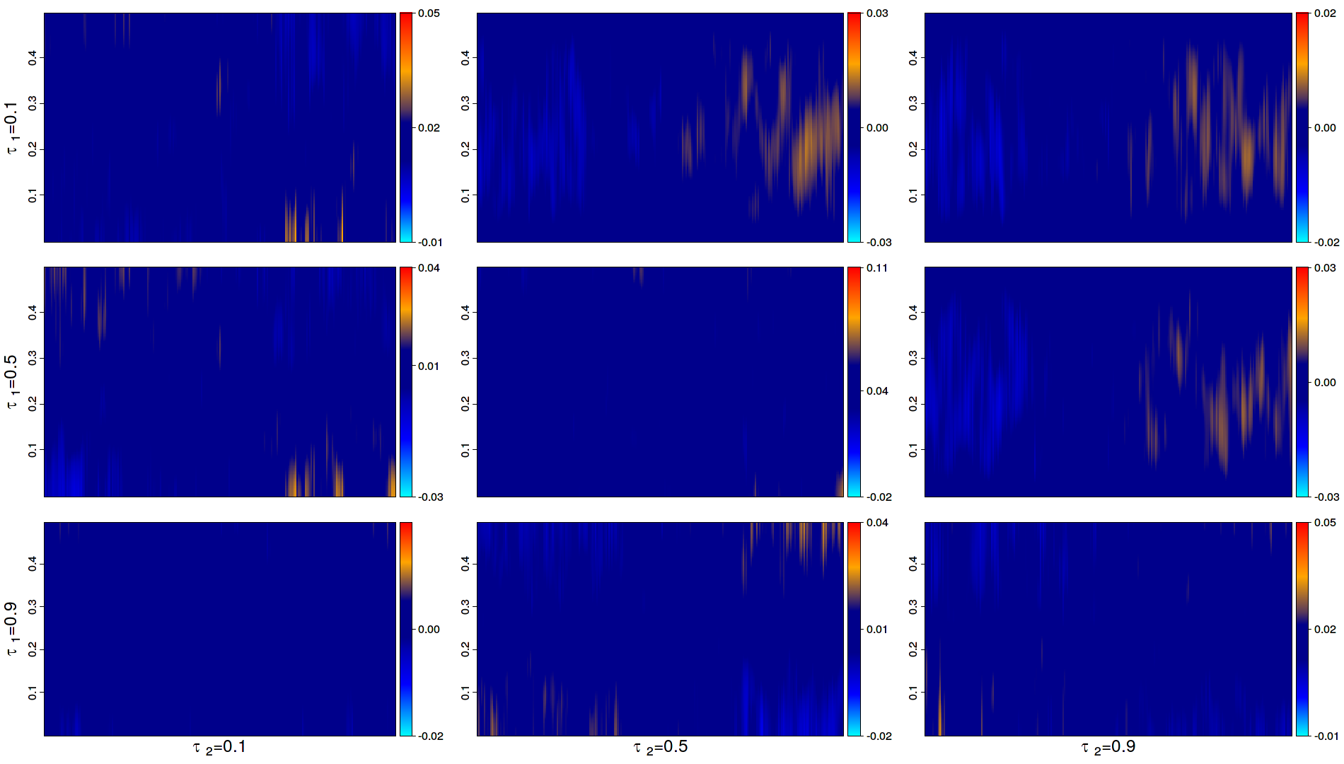
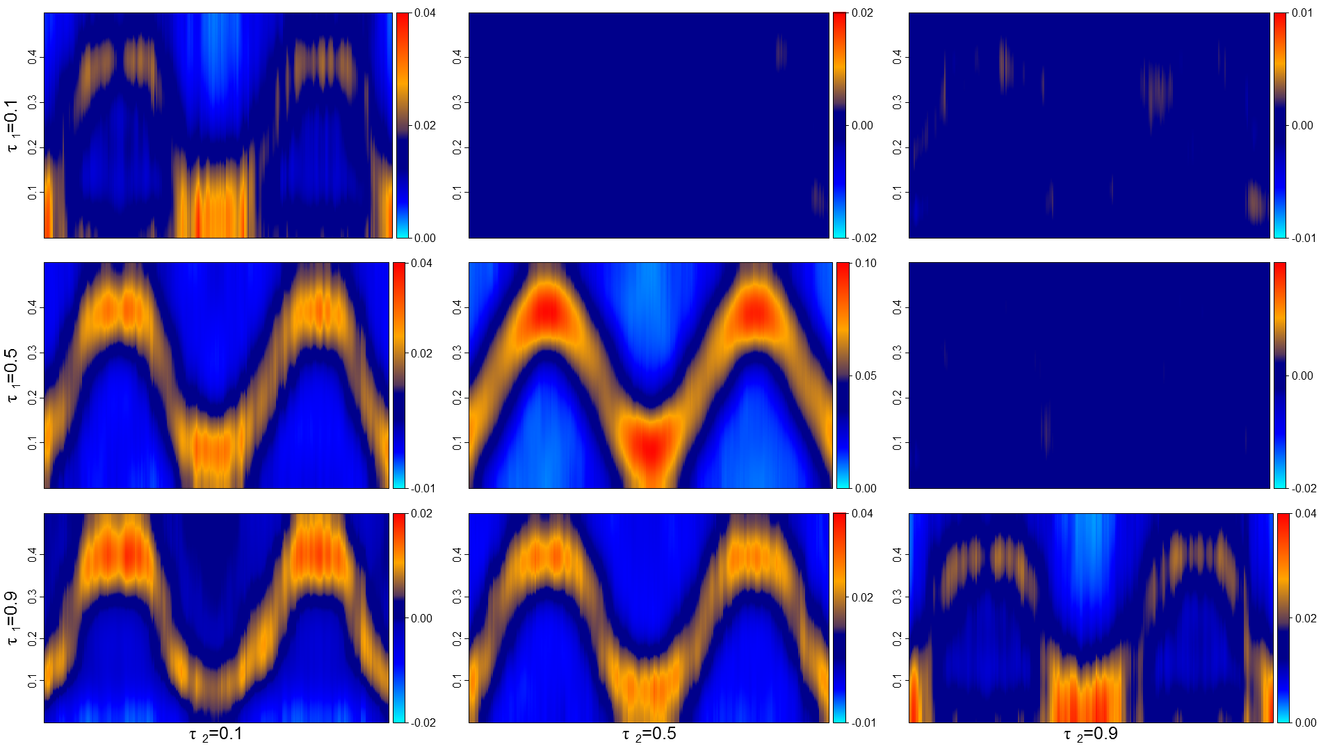
4.2.2 tvQAR(1)

Figure 4 shows the same heat diagrams for the QAR(1) (Quantile Autoregression) model of order one

$$X_{t,T}=[(1.9U_{t}-0.95)(t/T)+(-1.9U_{t}+0.95)(1-(t/T))]X_{t-1,T}+(U_{t}-1/2),\vspace{-2mm}$$

where the $U_{t}$’s are i.i.d.  uniform over $[0,1]$ (see Koenker and Xiao, (2006)). The corresponding strictly stationary approximation at $t_{0}=\vartheta T$, $0\leq\vartheta\leq 1$, is

$$X_{t}^{\vartheta}=[(1.9V_{t}-0.95)\vartheta+(-1.9V_{t}+0.95)(1-\vartheta)]X_{t-1}^{\vartheta}+(V_{t}-1/2)\vspace{-1mm}$$ (4.3)

where the $V_{t}$’s are i.i.d. uniform over $[0,1]$. The gradient of the coefficient function in (4.3) changes slowly from $1.9\,U_{t}-0.95$ to $-1.9\,U_{t}+0.95$, so that the spectral densities associated with the lower quantiles for small values of $t_{0}/T$ are the same as those associated with the upper quantiles for $1-t_{0}/T$, and vice versa.

This behavior, which cannot be detected via classical spectral methods, is quite visible here. Comparing the plots for $\tau=(0.5,0.1)$ and $\tau=(0.9,0.5)$, we see that the real parts reflect the behavior of the time-varying coefficient functions; mirroring one of them at a vertical axis in $\vartheta=0.5$ yields the other one. On the other hand, the imaginary parts are time-varying but stable over different quantile combinations.

Comparing Figure 4 with Figure 3 reveals completely different reactions to variations of window lengths. The tvAR$(2)$ case in Figure 3 indeed consists in a strong signal rapidly changing over time, whereas the signal in the tvQAR(1) of Figure 4 is rather weak and therefore harder to detect, with, however, a much smoother evolution in time. As a consequence, a larger window length yields better results in the estimation of the time varying spectral densities. The best results are obtained for $n=2048$, and the estimator displays most of the details found in the actual spectral density.

(a) Actual copula spectral densities (simulated)

(b) Estimated copula spectral densities, $n=128$

(c) Estimated copula spectral densities, $n=256$

(d) Estimated copula spectral densities, $n=512$

(e) Estimated copula spectral densities, $n=1024$

(f) Estimated copula spectral densities, $n=2048$

Figure 3: Heatmaps of the Cauchy time-varying AR(2) process described in Section 4.2.1 and the corresponding estimators, for various window lenghts.

(a) Actual copula spectral densities (simulated)

(b) Estimated copula spectral densities, $n=128$

(c) Estimated copula spectral densities, $n=256$

(d) Estimated copula spectral densities, $n=512$

(e) Estimated copula spectral densities, $n=1024$

(f) Estimated copula spectral densities, $n=2048$

Figure 4: Heatmaps of the time-varying QAR(1) process described in Section 4.2.2 and the corresponding estimators, for various window lenghts.

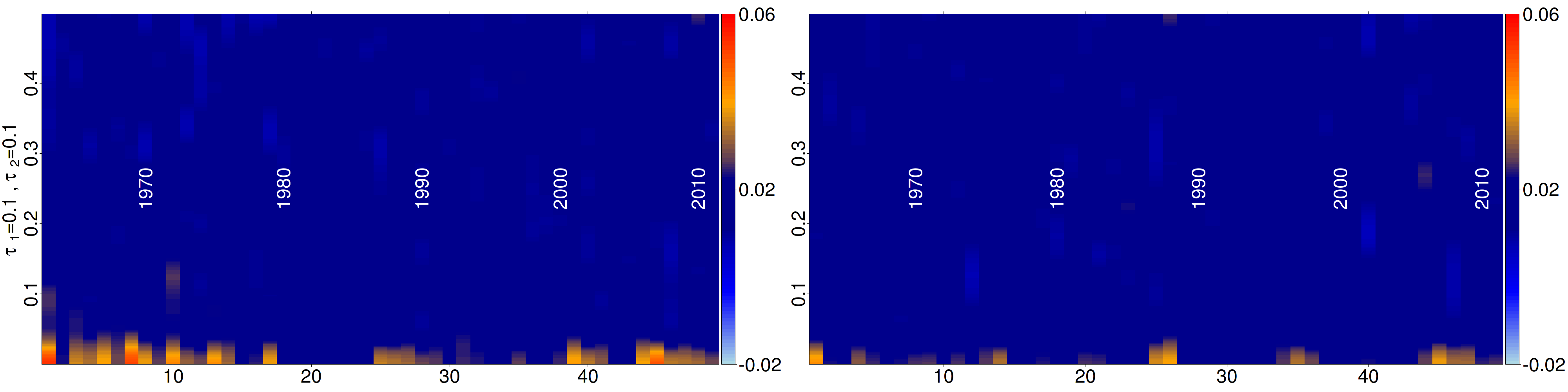
4.3 Standard & Poor’s 500

Figure 5: Time-frequency heatmaps of the quantile lag-window estimator for the log-returns from the S&P500 between 1962-2013 for quantile levels $0.1,0.5$ and $0.9$. The vertical axis represents frequencies ($0<\omega/2\pi<0.5$) and the horizontal axis is time ($1\leq t\leq 12992$). The plots are organized as explained in Section 4.1; the color code is provided along the right-hand side of each figure.

Figure 6: Time-frequency heatmaps of the quantile lag-window estimators for $\tau_{1}=\tau_{2}\in\{0.2,0.8\}$ (no imaginary parts, thus). The vertical axis represents the frequencies ($0<\omega/2\pi<0.5$) and the horizontal axis is time ($1\leq t\leq 12992$); for each value of $t$, a periodogram is plotted against frequencies via the color code provided along the right-hand side of each figure.

Figure 7: The $\tau_{1}=\tau_{2}=0.1$ local lag-window estimator of Figure 5; vertical dashed lines indicate historical financial crises, namely the Oil Crisis of 1973, the Black Monday (19.10.1987) which took place during the Savings and Loan Crisis in the USA, the bursting of the dot-com bubble in 2001 (followed by the early 2000s recession), and the 2007-2012 financial crisis.

We now turn back to the S&P500 index series already considered in the introduction, with $T=12992$ daily observations from 1962 through 2013 (differences of the logarithms of daily opening and closing prices for about 52 years). We applied the same estimation method as above, with the same window function as described in Section 4.2, with bandwidth $B_{n}=25$, window length $n=512$, and the sets ${\cal T}_{0}=\{256+256j|0\leq j\leq 49\}$ and $\Omega=\{2\pi j/256|j=0,...,255\}.$ Calibration was performed as explained in Section 4.1. The resulting heatmaps are shown in the heatmaps of Figure 5.

Whereas the central heatmaps ($\tau_{1}=\tau_{2}=0.5$) are pretty flat (uniform dark blue) with the exception of some deviations from white noise behavior limited to the early seventies, the more extreme ones ($\tau_{1}=\tau_{2}=0.1$ and $0.9$) suggest an alternance of high low-frequency spectral densities (yellow and red) and perfectly ‘flat’ (dark blue) periods. A closer analysis reveals that those periods of strong dependence in the tails typically correspond to well-identified crises and booms (see below for details). Another interesting observation is the marked asymmetry between the time-varying spectra associated with the left ($\tau=0.1$) and right ($\tau=0.9$) tails, which can be interpreted in terms of prospect theory (see Kahneman and Tversky, (1979)). That asymmetry is confirmed by comparing the estimated spectra for $\tau=0.2$ and $\tau=0.8$ (see Figure 6); again, it cannot be detected by covariance-based methods. Inspection of local stationary copula-based spectra thus suggests that the S&P500 series is not as close to white noise as claimed. However, it takes a combination of quantile-related and local stationarity tools to bring some evidence for that fact.

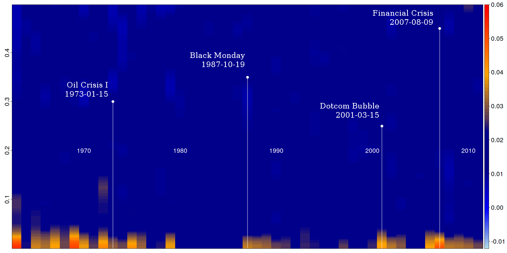
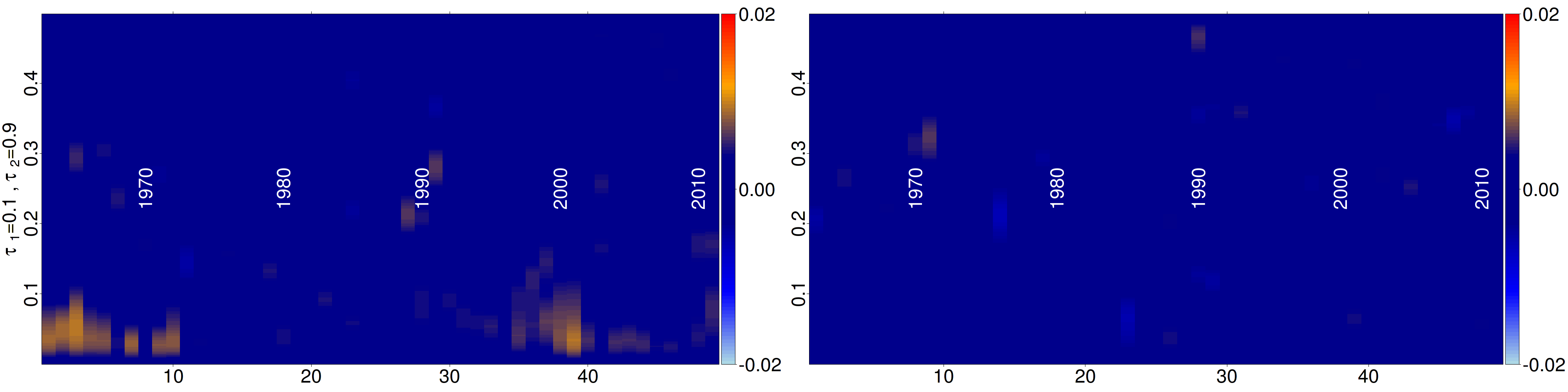
We now take a closer look at deviations from the white noise behavior (dark blue) which are particularly visible in the diagrams associated with tail quantile levels. Concentrating on the $\tau_{1}=\tau_{2}=0.1$ case, closer inspection of the diagram reveals a relation between low-frequency spectral peaks and financial crisis events: in Figure 7, vertical white lines are identifying the Oil Crisis of 1973, the Black Monday (19.10.1987) which took place during the Savings and Loan Crisis in the USA, the bursting of the dot-com bubble in 2001 (followed by the early 2000s recession), and the 2007-2012 financial crisis. Those episodes clearly are matching most of the low-frequency peaks quite well, indicating that crises lead to, or consist of, strong changes in the dependence structure of low returns.

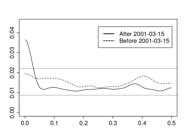
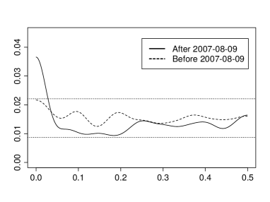
This apparent impact of crises on copula spectra is confirmed when focusing the analysis on the corresponding periods. In Figure 8, we provide plots of the local lag-window estimators for $\tau_{1}=\tau_{2}=0.1$ before and after two of those four crises, the 2001 bursting of the dot-com bubble and the 2007 financial crisis. More precisely, for each of them, we calculated local lag-window estimations using only observations before the critical date, and compared them to estimations using only observations taken after it. None of the pre-crisis curves indicates any significant deviation from white noise, whereas both post-crisis ones do. The interpretation is that crises, locally but quite suddenly, produce changes in the dependencies between low returns. Those changes happen after the crisis onset, and thus do not help predict ing them; as shown by Figure 7, they fade away more slowly than they appeared. As for the atypical spectra in the late sixties, they are probably due to the fact that the market, at that time, was much smaller, and less efficient, than nowadays. In addition, some of the peaks of low-returns spectral densities at low frequencies are not systematically associated with any well-identified crisis. This indicates that, apart from crises, other events can also influence the dependence structure of low returns. Peaks in quantile spectral densities at low frequencies, indeed, also can be caused by time-varying variances. This fact was first observed by Li, (2014), who suggested that this phenomenon could explain some features of the S&P500 spectra. A closer look, however, reveals that it cannot account for all dependence in that dataset: see Section A.3.1 of the online appendix.

Figure 8: Single local lag-window estimators calculated before (dashed) and after (solid) the bursting of the dot-com bubble in 2001 (left) and the beginning of the financial crisis in 2007 (right); the dotted horizontal lines represent the values of $q_{\min}$ and $q_{\max}$ from Section $\ref{Seccalibr}(iii);$ smoothing and bandwidth choices as in Figure 5.

4.4 Daily temperatures in Hohenpeissenberg

Figure 9: First row displays $T=11315$ observation of daily mean temperature between 1985 and 2015 at the Hohenpeissenberg Meteorological Observatory and its autocorrelation function; the second row shows the residuals of the ARMA$(3,1)$ fit and its autocorrelation function.

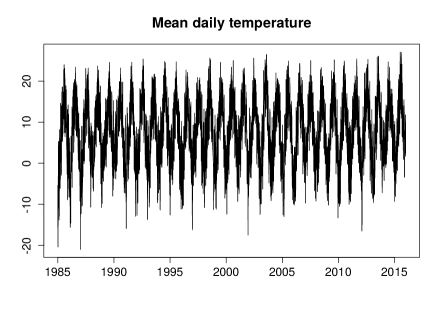
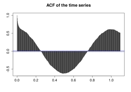
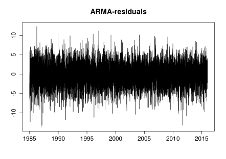
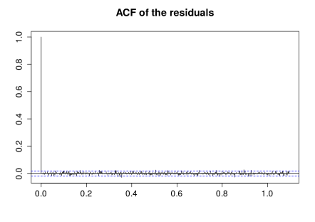
As mentioned in Section 4.1, the new methodology admits a hypothesis testing interpretation—the null hypothesis being that of strong white noise. In our second dataset, we analyze the residuals of an ARMA$(p,q)$ fit to a seasonally adjusted time-series of air temperatures recorded at the meteorological station in Hohenpeissenberg (Germany). More precisely, $T=11315$ observations of daily mean temperatures were recorded between 1985 and 2015; they are displayed in the upper part of Figure 9. To remove the clearly visible seasonality , we first fit a trigonometric regression model of the form

$$y=c+\alpha x+\sum_{k=1}^{4}\beta_{k}\sin(2\pi k/365)+\gamma_{k}\cos(2\pi k/365),$$

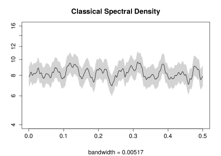
where the linear part is used to remove any possible trend. An ARMA(p,q) model with $p=3$ and $q=1$ (determined via $AIC$ and an inspection of residual autocorrelations, see Campbell and Diebold, (2011) for a similar approach) then was estimated from the residuals. The residuals resulting from that second fit and their autocorrelations are shown in the lower part of Figure 9. From a $L_{2}$ perspective, this successfully captures the bivariate behavior of the dataset. It its therefore not surprising that the (global) classical spectral density of those residuals does not show any significant structure (see Figure 10).

Figure 10: Classical spectral density of the ARMA-residuals with pointwise calculated $0.95$ confidence interval .

The quantile spectral analysis of the same dataset leads to a much different conclusion. Estimating the quantile spectral densities of the same residuals with $B_{n}=10,$ $n=2048,$ $\mathcal{T}_{0}=\{1024+32j|j=0,\dots,290\}$, and $\Omega=\{2\pi j/1024|j=0,\dots,1023\}$, we obtain the heat maps shown in Figure 11. The central heat map ($\tau_{1}=\tau_{2}=0.5$ deviates) indicates clear deviations from strong white noise. Starting around 1995, a significant peak around frequency zero appears. The peak reaches its maximum in 2003 and declines slowly afterwards but does not vanish. It is interesting to note that this peak is most prominent during the 2003 heat wave in Europe, which could indicate a connection with long-term climatic fluctuations. Other significant effects, although not as dramatic, are also visible in the heat maps involving more extreme quantiles $\tau_{1},\tau_{2}\in\{0.1,0.9\}$. One interesting observation is the strong asymmetry between the spectra associated with low and high temperatures (quantiles).

These results suggest that an ARMA model is far from fully capturing the distributional features of the data—though it does capture its $L^{2}$ dynamics. The analysis performed here reveals clear deviations from white noise, which again cannot be detected by classical spectral analysis. It also clearly shows an evolution through time of the dependence structure of daily temperatures. Such findings are not entirely new, and ARMA-GARCH models have been proposed for similar datasets: see Campbell and Diebold, (2011). It should be emphasized, however, that the residual spectra we observe in this dataset do not correspond to typical GARCH spectra, which suggests that it might be worthwhile to investigate the validity of such parametric models in greater detail.

Figure 11: Time-frequency heatmaps of the quantile lag-window estimator for the ARMA-residuals of the daily mean temperature between 1985 and 2015 at the Hohenpeissenberg Meteorological Observatory for quantile levels $0.1,0.5$ and $0.9$. The vertical axis represents frequencies ($\omega/2\pi$, ranging from 0 to 0.5), and the horizontal axis is time ($1\leq t\leq 11315$). The plots are organized as explained in Section 4.1; the color code is provided along the right-hand side of each figure.

5 Theoretical results

5.1 Examples of locally strictly stationary models

In contrast with the many definitions of local stationarity considered in the literature, which are based on evolving covariance structures, and classical spectra, or time-varying parametric models, local strict stationarity is a purely distributional concept. In this section, we show how, under additional constraints, those other concepts eventually fall under the umbrella of our definition.

5.1.1 tvMA$(\infty)$ processes.

Dahlhaus and Polonik, (2006) define a tvMA$(\infty)$ process as admitting a representation of the form

$$X_{t,T}=\mu(t/T)+\sum_{j=-\infty}^{\infty}a_{t,T}(j)\xi_{t-j},$$ (5.1)

where $\xi_{t}$ is i.i.d. white noise. This definition cover a wide range of popular linear time-varying models, such as the tvARMA$(p,q)$ ones.

Consider the following assumptions.

(MA1)

There exist functions $a(\cdot,j)$ and $\mu(\cdot):(0,1)\rightarrow\mathbb{R}$ with

$$\sup_{t,T}|a_{t,T}(j)-a(\frac{t}{T},j)|\leq\frac{K}{Tl(j)},\quad\sup_{u\in(0,1)}\left|\frac{\partial a(u,j)}{\partial u}\right|\leq\frac{K}{l(j)},\text{ and }\sup_{u\in(0,1)}\left|\frac{\partial\mu(u)}{\partial u}\right|\leq K$$

1. where $K$ is a finite constant (not depending on $j$) and $\sum_{j}1/l(j)<\infty.$ Furthermore, $\sup_{u\in(0,1)}\sum_{j=-\infty}^{\infty}|a(u,j)|<\infty$ and $\inf_{u\in(0,1)}|a(u,0)|>\rho>0.$

(MA2)

The random variables $\xi_{t}$ have bounded density function $f_{\xi}$ and finite expectation, and, for some constant $C_{f}>0$, $f_{\xi}$ is such that $\sup_{x\in\mathbb{R}}|xf_{\xi}(x)|\leq C_{f}.$

We then have the following result.

Lemma 5.1.

If Assumptions (MA1) and (MA2) hold, the tvMA$(\infty)$ process defined in $(\ref{def:MA})$ is locally strictly stationary in the sense of Definition 2.1, with stationary approximation

$$X^{\vartheta}_{t}=\mu(\vartheta)+\sum_{j=-\infty}^{\infty}a(\vartheta,j)\zeta_{t-j}\vspace{-3mm}$$

where the $\zeta_{t}$’s are i.i.d. copies of the $Z_{t}$’s.

5.1.2 tvARCH$(\infty)$processes.

Dahlhaus and Subba Rao, (2006) define a tvARCH$(\infty)$ process by

$$X_{t,T}=\sigma_{t,T}Z_{t},\qquad\text{where}\qquad\sigma_{t,T}^{2}=a_{0}(t/T)+\sum_{j=1}^{\infty}a_{j}(t/T)X^{2}_{t-j,T},\vspace{-1mm}$$ (5.2)

where the $Z_{t}$’s are i.i.d. random variables with $\mathbb{E}(Z_{t})=0,\mathrm{Var}(Z_{t})=1,$ and density $f.$ They show that $X^{2}_{t,T}$, if not $X_{t,T}$ itself, has an almost surely well-defined and unique expression in the set of all causal solutions of (5.2) if the following assumption holds.

(ARCH1)

The coefficients $a_{j}$ in (5.2) are non-negative and $\inf_{u\in(0,1)}a_{0}(u)>\rho$ for some constant $\rho>0.$ There exist constants $Q<\infty$, $M<\infty$, and $0<\nu<1$, and a positive sequence $l(j)$, $j\in\mathbb{N}$, such that $\sum_{j=1}^{\infty}{j}/{l(j)}<\infty,$ and

$$\sup_{u\in(0,1)}a_{j}(u)<{Q}/{l(j)},\quad Q\sum_{j=1}^{\infty}{1}/{l(j)}\leq(1-\nu)\text{ and }|a_{j}(u)-a_{j}(v)|<M{|u-v|}/l(j).$$

In general, equation $(\ref{def:tvARCH})$ has no unique solution, as the sign of a solution $X_{t,T}$ associated with the almost surely well-defined (under assumption $(ARCH1)$) $X^{2}_{t,T}$ can be randomly either positive or negative. To avoid this non-unicity problem, we require $\sigma_{t,T}$ in (5.2) to be positive. More precisely, we impose the following condition.

(ARCH2)

For some constant $C_{f}<\infty$, $\sup_{x\in\mathbb{R}}|xf(x)|<C_{f}$, and $\sigma_{t,T}=\sqrt{\sigma_{t,T}^{2}}.$

We then have the following result.

Lemma 5.2.

If Assumptions (ARCH1) and (ARCH2) hold, a process $X_{t,T}$ satisfying equation $(\ref{def:tvARCH})$ is locally strictly stationary in the sense of Definition 2.1, with stationary approximation

$$X^{\vartheta}_{t}=\sigma^{\vartheta}_{t}\zeta_{t}\qquad\text{with}\qquad(\sigma^{\vartheta}_{t})^{2}=a_{0}(\vartheta)+\sum_{j=1}^{\infty}a_{j}(\vartheta)(X^{\vartheta}_{t-j})^{2}\vspace{-3mm}$$

where the $\zeta_{t}$’s are i.i.d. copies of the $Z_{t}$’s.

5.1.3 tvGARCH$(p,q)$ processes.

Subba Rao, (2006) similary defines a tvGARCH$(p,q)$ process as

$$X_{t,T}=\sigma_{t,T}Z_{t},\quad\text{with}\quad\sigma_{t,T}^{2}=a_{0}(t/T)+\sum_{j=1}^{p}a_{j}(t/T)X^{2}_{t-j,T}+\sum_{i=1}^{q}b_{j}(t/T)\sigma^{2}_{t-j,T},$$ (5.3)

where $Z_{t}$ are i.i.d. random variables with $\mathbb{E}(Z_{t})=0$, $\mathrm{Var}(Z_{t})=1$, and density $f.$ Parallel to (ARCH1) and (ARCH2), consider the following assumptions.

(GARCH1)

The coefficient functions $a_{j}(u)$, $j=0,\ldots,p$ and $b_{j}(u)$, $j=1,\ldots,q$, are positive, Lipschitz-continuous, and satisfy, for some $0<\mu<1$ and $\rho>0$,

$$\sup_{u\in(0,1)}\Big{[}\sum_{j=1}^{p}a_{j}(u)+\sum_{i=1}^{q}b_{j}(u)\Big{]}<1-\mu,\quad\text{and}\quad\inf_{u\in(0,1)}a_{0}(u)>\rho.$$ (5.4)

(GARCH2)

For some constant $C_{f}<\infty$, $\sup_{x\in\mathbb{R}}|xf(x)|\leq C_{f}$, and $\sigma_{t,T}=\sqrt{\sigma_{t,T}^{2}}$.

The following then holds true.

Lemma 5.3.

If Assumptions (GARCH1) and (GARCH2) hold, a process $X_{t,T}$ satisfying equation $(\ref{def:tvGARCH})$ is locally strictly stationary in the sense of Definition 2.1, with stationary approximation

$$X^{\vartheta}_{t}=\sigma^{\vartheta}_{t}\zeta_{t},\quad\text{ where }\quad(\sigma^{\vartheta}_{t})^{2}=a_{0}(\vartheta)+\sum_{j=1}^{p}a_{j}(\vartheta)(X^{\vartheta}_{t-j})^{2}+\sum_{i=1}^{q}b_{j}(\vartheta)(\sigma^{\vartheta}_{t-j})^{2}\vspace{-3mm}$$

and the $\zeta_{t}$’s are i.i.d. copies of the $Z_{t}$’s.

The proofs of Lemmas 5.1-5.3 can be found in Section A.4.1 of the online appendix.

5.2 Asymptotic theory

Let $(\Omega,\mathscr{A},\mathbb{P})$ denote a probability space, and let $\mathscr{B}$, and $\mathscr{C}$ be subfields of $\mathscr{A}.$ Define

$$\beta(\mathscr{B},\mathscr{C}):=\mathbb{E}\sup_{C\in\mathscr{C}}|\mathbb{P}(C)-\mathbb{P}(C|\mathscr{B})|$$

and, for an array $\{Z_{t,T}:1\leq t\in\mathbb{Z}\}$, let

$$\beta(k):=\sup_{T}\sup_{t\in\mathbb{Z}}\beta(\sigma(Z_{s,T},s\leq t),\sigma(Z_{s,T},t+k\leq s)),\vspace{-2mm}$$

where $\sigma(Z)$ is the $\sigma-$field generated by $Z.$ Recall that a process is called $\beta$-mixing or absolutely regular if $\beta(k)\rightarrow 0$ as $k\rightarrow\infty.$

Before proceeding with the asymptotic properties of $\hat{\mathfrak{f}}_{t_{0},T}(\omega,\tau_{1},\tau_{2})$, we are collecting here some technical assumptions needed in the sequel.

1. The lag-window function $K$ in $(\ref{esti})$ satisfies $\|K\|_{\infty}\leq 1$, $K(0)=1$ and has support $[-1,1];$ its extension to $\mathbb{R}$ is $d$ times continuously differentiable with $d\geq 2$. Additionally, $K$ has ‘characteristic exponent’ $r>0$ [see Parzen, (1957) or Priestley, (1981)], that is, $r$ is the largest integer such that $C_{K}(r):=\lim_{u\to 0}\big{(}{1-K(u)}\big{)}/{|u|^{r}}$ exists, is finite and non-zero.

1. The triangular array $\{X_{t,T}\}$ is $\beta$-mixing with mixing coefficients $\beta^{[X]}(k)=O(k^{-\delta})$ for some $\delta>1$. The same holds for $\{X_{t}^{\vartheta}\}$.

2. For any $\varepsilon>0$ define $\rho_{n}(\varepsilon):=\big{(}\frac{\varepsilon+n^{{1}/{(1+\delta)}}\varepsilon^{2}}{n}\log(n)\big{)}^{{1}/{2}}\vee(n^{-{\delta}/{(1+\delta)}}\log(n)),$ with $\delta$ as in Assumption (A1). Assume that $\rho_{n}(T^{-2/5})=o((nB_{n})^{-1/2})$, $T^{-2/5}=o(B_{n}^{1/2}/n^{1/2})$ and

   $$\frac{B_{n}^{2}}{n}+\frac{n^{2}}{T^{2}B_{n}}+\frac{n^{1/2}B_{n}}{T}=o\Big{(}\frac{B_{n}^{1/2}}{n^{1/2}}\Big{)}.$$

3. 1. For some $\gamma>2$ and $T^{-2(\gamma-1)/5\gamma}=o(B_{n}^{1/2}n^{-1/2}),$

      $$\sup_{t}\sup_{x,y}\Big{|}F_{t,t+k;T}(x,y)-F_{t;T}(x)F_{t+k;T}(y)\Big{|}=O(|k|^{-\gamma}).$$

   2. $\sum_{k\in\mathbb{Z}}|k|^{r}\sup_{u,\eta_{1},\eta_{2}}|\gamma^{u}_{k}(\eta_{1},\eta_{2})|<\infty\vspace{1mm}$, where the supremum is over a neighborhood of $(\vartheta,q^{\vartheta}(\tau_{1}),q^{\vartheta}(\tau_{2}))$.

   3. For $2\leq p\leq 8$, define

      $$\kappa_{p}(s_{1},...,s_{p-1}):=\sup_{T}\sup_{t\in\mathcal{N}_{t_{0},T}}\sup_{x_{1},...,x_{p}}|\mathrm{cum}(\mathbb{I}_{\{X_{t,T}\leq x_{1}\}},\mathbb{I}_{\{X_{t+s_{1},T}\leq x_{2}\}},...,\mathbb{I}_{\{X_{t+s_{p-1},T}\leq x_{p}\}})|$$

      $$\kappa_{p}^{\vartheta}(s_{1},...,s_{p-1}):=\sup_{x_{1},...,x_{p}}|\mathrm{cum}(\mathbb{I}_{\{X_{0}^{\vartheta}\leq x_{1}\}},\mathbb{I}_{\{X_{s_{1}}^{\vartheta}\leq x_{2}\}},...,\mathbb{I}_{\{X_{s_{p-1}}^{\vartheta}\leq x_{p}\}})|;\vspace{-2mm}$$

      assume moreover that the quantities $\kappa_{p}(s_{1},...,s_{p-1})$ and $\kappa_{p}^{\vartheta}(s_{1},...,s_{p-1})$ are absolutely summable over $s_{1},...,s_{p-1}\in\mathbb{Z}$.

4. 1. The joint distribution functions $F_{t_{1},...,t_{j};T}$ of $(X_{t_{1};T},...,X_{t_{j};T}),j=2,...,4$ are twice continuously differentiable, and all partial derivatives of order one and two are bounded, uniformly in $t_{1},...,t_{j},T$ and the arguments. The distribution function $F_{t_{1};T}$ is twice continuously differentiable and its derivatives are bounded uniformly in $t_{1}$ and $T$.

   2. Let $\mathfrak{d}^{(r)}_{\omega}\mathfrak{f}^{u}(\omega,x,y):=\frac{1}{2\pi}\sum_{k\in\mathbb{Z}}|k|^{r}\gamma^{u}_{k}(x,y)e^{-\mathrm{i}k\omega},$ where $r$ is taken from Assumption (K). The function $(u,x,y)\mapsto\mathfrak{d}^{(r)}_{\omega}\mathfrak{f}^{u}(\omega,x,y)$ is continuous in a neighborhood of $(u,x,y)=(\vartheta,q^{\vartheta}(\tau_{1}),q^{\vartheta}(\tau_{2}))$.

   3. The function $u\mapsto\mathfrak{f}^{u}(\omega,G^{u}(q^{\vartheta}(\tau_{1})),G^{u}(q^{\vartheta}(\tau_{2})))$ is twice continuously differentiable in a neighborhood of $u=\vartheta$.

   4. The functions $G^{u}_{k}$ and $G^{u}$ in the definition of local strict stationarity are, for some $d\geq 2,$ $d$ times continuously differentiable with respect to $u.$ The function $G^{\vartheta}$ has a density, which is uniformly bounded away from zero on an open set that contains $q^{\vartheta}(\tau_{1})$ and $q^{\vartheta}(\tau_{2})$.

Remark 5.1.

Assumptions (K) and (A2) place mild restrictions on the lag-window generator $K$ and the bandwidth parameter, respectively. One can show that they are satisfied by the bandwidth parameters leading to optimal asymptotic MSE rates for the mean squared error, see the discussion in Remark 5.3 for more details. Assumption (A3) is verified if $\delta$ in (A1) is large enough: in fact, it is sufficient to replace the $\beta$-mixing coefficients in (A1) by $\alpha$-mixing coefficients (see Lemma A.5.1 in the online Appendix for additional details on bounding cumulants through $\alpha$-mixing coefficients). Assumption (A4) places conditions on the smoothness properties of the underlying processes which rule out processes with jump-like non-stationarity.

Remark 5.2.

Observe that

$$\mathfrak{f}^{u}\big{(}\omega,G^{u}(q^{\vartheta}(\tau_{1})),G^{u}(q^{\vartheta}(\tau_{2})\big{)}=\frac{1}{2\pi}\sum_{k\in\mathbb{Z}}e^{-ik\omega}\big{(}G^{u}_{k}(q^{\vartheta}(\tau_{1}),q^{\vartheta}(\tau_{2}))-G^{u}(q^{\vartheta}(\tau_{1}))G^{u}(q^{\vartheta}(\tau_{2}))\big{)}.$$

This means that the differentiability of $u\mapsto\mathfrak{f}^{u}(\omega,G^{u}(q^{\vartheta}(\tau_{1})),G^{u}(q^{\vartheta}(\tau_{2})))$ depends on the local smoothness with respect to time of joint distributions.

Our main result states that, after proper centering and scaling, $\hat{\mathfrak{f}}_{t_{0},T}(\omega,\tau_{1},\tau_{2})$ is asymptotically (complex) normal.

Theorem 5.1.

Let Assumptions (K) and (A1)-(A4) hold. Then, for any sequence $\omega_{n}$ of Fourier frequencies such that $|\omega_{n}-\omega|=O(1/n)$ for some $\omega\in(0,\pi)$, and for $t_{0}=\lfloor T\vartheta\rfloor$,

$$\sqrt{n/B_{n}}\Bigg{(}\begin{array}[]{c}\Re\hat{\mathfrak{f}}_{t_{0},T}(\omega_{n},\tau_{1},\tau_{2})-\Re\mathfrak{f}^{\vartheta}(\omega,\tau_{1},\tau_{2})-\Re b(\omega,\tau_{1},\tau_{2})\\ \Im\tilde{\mathfrak{f}}_{t_{0},T}(\omega_{n},\tau_{1},\tau_{2})-\Im\mathfrak{f}^{\vartheta}(\omega,\tau_{1},\tau_{2})-\Im b(\omega,\tau_{1},\tau_{2})\end{array}\Bigg{)}\stackrel{{\scriptstyle\mathcal{D}}}{{\longrightarrow}}\mathcal{N}\Big{(}0,\Sigma^{2}(\omega,\tau_{1},\tau_{2})\Big{)}$$ (5.5)

where

$$\Sigma^{2}(\omega,\tau_{1},\tau_{2}):=\pi\mathfrak{f}^{\vartheta}(\omega,\tau_{1},\tau_{1})\mathfrak{f}^{\vartheta}(\omega,\tau_{2},\tau_{2})\int K^{2}(u)du\Big{(}\begin{array}[]{cc}1&0\\ 0&1\end{array}\Big{)}$$

and $$b(\omega,\tau_{1},\tau_{2}) :=-C_{K}(r)B_{n}^{-r}\mathfrak{d}^{(r)}_{\omega}\mathfrak{f}^{\vartheta}(\omega,\tau_{1},\tau_{2})$$

$$\hskip 28.45274pt+\frac{n^{2}}{2T^{2}}\frac{\partial^{2}}{\partial u^{2}}\mathfrak{f}^{u}(\omega,G^{u}(q^{\vartheta}(\tau_{1})),G^{u}(q^{\vartheta}(\tau_{2})))\Big{|}_{u=\vartheta}+o(B_{n}^{-r}+\frac{n^{2}}{T^{2}}).$$

Remark 5.3.

Theorem 5.1 implies consistency of the estimator, which, however, holds under weaker assumptions. The same theorem also can be used to obtain the local window length $n$ and the bandwidth parameter $B_{n}$ that minimize the asymptotic mean squared error of $\hat{\mathfrak{f}}_{t_{0},T}(\omega_{n},\tau_{1},\tau_{2})$. To illustrate the idea, assume that we want to optimize the asymptotic mean squared error (MSE) of $\Re\hat{\mathfrak{f}}_{t_{0},T}(\omega_{n},\tau_{1},\tau_{2})$. Considering $r=d$, let $\sigma^{2}:=\Sigma^{2}_{11}(\omega,\tau_{1},\tau_{2}),$

$$b_{u}:=\frac{1}{2}\frac{\partial^{2}}{\partial u^{2}}\mathfrak{f}^{u}(\omega,G^{u}(q^{\vartheta}(\tau_{1})),G^{u}(q^{\vartheta}(\tau_{2})))\Big{|}_{u=\vartheta}\quad\text{and}\quad b_{\omega}:=-C_{K}(r)\mathfrak{d}^{(r)}_{\omega}\mathfrak{f}^{\vartheta}(\omega,\tau_{1},\tau_{2}).\vspace{-1mm}$$

In this notation the asymptotic MSE of $\Re\hat{\mathfrak{f}}_{t_{0},T}(\omega_{n},\tau_{1},\tau_{2})$ is $\frac{B_{n}}{n}\sigma^{2}+b_{u}\frac{n^{2}}{T^{2}}+b_{\omega}B_{n}^{-r}$. Assuming that $b_{u}\neq 0$ and $b_{\omega}\neq 0$, straightforward calculations entail that this MSE is minimized for

$$n=T^{\frac{2+4r}{2+5r}}\big{(}\sigma^{2}b_{\omega}^{-1/r}b_{u}^{2+1/r}(2r+4)\big{(}\tfrac{r}{2}\big{)}^{\frac{-r}{r+1}}\big{)}^{\frac{r}{2+5r}},~{}B_{n}=T^{\frac{2}{2+5r}}\big{(}\sigma^{-2}b_{u}^{-1/2}b_{\omega}^{5/2}(2r+4)\big{)}^{\frac{2}{2+5r}}\big{(}\tfrac{2}{r}\big{)}^{\frac{-3}{2+5r}}.\vspace{-2mm}$$

As one would expect, larger values of $r,$ corresponding to smoother local spectral densities (as functions of frequency), lead to more smoothing and faster convergence rates. For $r=2$, the asymptotic MSE of $\hat{\mathfrak{f}}_{t_{0},T}(\omega_{n},\tau_{1},\tau_{2})$ turns out to be of the order $T^{-2/3}$. One can show that, if the constant $\delta$ in Assumption (A1) is large enough, the above choices of the bandwidth parameters satisfy condition (A2) if $r\geq 2$. The above formulas provide rough guidelines about the choice of smoothing parameters. However, the expression for the bias contains unknown parameters, such as derivatives of the local copula spectral density kernel, which are difficult to estimate in practice.

6 Conclusions

In this paper, we have defined local copula spectra using a new notion of local strict stationarity; we have constructed a lag-window type estimator and proved its asymptotic normality. In a stationary context, it has been shown that copula-based spectra provide a description of serial dependence structures which is substantially more informative and flexible than classical covariance-based spectra. The benefits of this new spectral methodology are thus extended to slowly evolving dependence structures. Those benefits are highlighted in a simulation study and by analyzing two datasets, the daily log-returns of the classical S&P500 series and a meteorological series recorded in Hohenpeissenberg. That analysis indeed reveals a number of interesting features that cannot be detected by a more traditional $L^{2}$-based approach.

Several important questions are calling for further research, though. Our method requires the choice of a smoothing parameter—an issue which is common to all methods based on local stationarity concepts. It seems important to have some data-driven procedure providing general guidelines on what a ‘good’ choice of smoothing parameters is. An interesting approach to this problem has been suggested recently by Cranstoun et al., (2002), and an important direction for future research is the extension of this method to the present setting. It also is important to develop methods for uniformly (in frequency and local time) valid statistical inference on quantile spectra. This is challenging, and to the best of our knowledge such methodology for the simpler case of classical $L^{2}$ spectra has only recently been developed by Liu and Wu, (2010) in the stationary case. Finally, it is natural to assume that the dependence structure of a time series contains both smooth changes and sudden jumps. In the present paper, we have dealt with smooth changes only, and an extension accommodating possible jumps would be most welcome. For example, in an $L^{2}$ setting, such smoothness assumptions could be avoided using the piecewise locally stationary concept of Zhou, (2013) or by considering the evolutionary wavelet spectra as described in Van Bellegem and Von Sachs, (2008). Extending the distributional approach described in this paper to piecewise locally stationary processes or wavelet-based spectra (even in a strictly stationary case) is an interesting and challenging direction for future research.

Acknowledgements. We gratefully acknowledge the many suggestions and constructive comments by two Referees, an Associate Editor and an Editor, that helped improving the original version of this paper.

Online Appendix

In this online appendix, we collect (Section A.1) some additional information on the spectral concept considered here, (Section A.2) some additional simulation results, (Section A.3) some further analysis of the S&P500 data, and (Section A.1) (Sections A.4-A.6) the proofs of the main results, along with some technical details.

A.1 A connections with the Wigner-Ville spectra

A further theoretical justification for the time-varying copula spectral density kernels considered in this paper is their relation to the so-called Wigner-Ville spectrum. The Wigner-Ville spectrum (in its classical L² version) is based on the so-called Wigner distribution of a process of the form $\{X_{t,T}\}$ and has its origins in quantum mechanics. It was used later on in the signal processing community. Its properties for time-varying spectral analysis have been investigated in Martin and Flandrin, (1985).

For the series of indicators we are dealing with here, the Wigner-Ville spectrum takes the form

$$\mathfrak{W}_{t_{0},T}(\omega,\tau_{1},\tau_{2}):=\sum_{s=-\infty}^{\infty}\mathrm{Cov}\Big{(}\mathbb{I}_{\{X_{\lfloor t_{0}+s/2\rfloor,T}\leq F^{-1}_{\lfloor t_{0}+s/2\rfloor;T}(\tau_{1})\}},\mathbb{I}_{\{X_{\lfloor t_{0}-s/2\rfloor,T}\leq F^{-1}_{\lfloor t_{0}-s/2\rfloor;T}(\tau_{2})\}}\Big{)}\frac{e^{-i\omega s}}{2\pi}\vspace{-3mm}$$ (A.1)

(see Martin and Flandrin, (1985)).

The following proposition establishes a strong relation between our time-varying copula spectral density kernels $\mathfrak{f}^{\vartheta}(\omega,\tau_{1},\tau_{2})$, as defined in $(\ref{def:tvf})$, and the Wigner-Ville spectrum $\mathfrak{W}_{t_{0},T}(\omega,\tau_{1},\tau_{2})$.

Proposition A.1.1.

Let $\{X_{t,T}\}$ be locally strictly stationary, with approximating processes $\{X^{\vartheta}_{t}\}$, and assume that Assumption (A1) holds. If moreover the $\gamma_{h}^{\vartheta}(\tau_{1},\tau_{2})$’s are absolutely summable for any $\vartheta$ and $(\tau_{1},\tau_{2})\in(0,1)^{2}$, then, for any fixed $\vartheta$ and $(\tau_{1},\tau_{2})\in(0,1)^{2}$, along any sequence $t_{0}=t_{0}(T)$ such that $t_{0}/T~{}\!\!\to~{}\!\vartheta$,

$$\sup_{\omega\in(-\pi,\pi]}\Big{|}\mathfrak{f}^{\vartheta}(\omega,\tau_{1},\tau_{2})-\mathfrak{W}_{t_{0},T}(\omega,\tau_{1},\tau_{2})\Big{|}=o(1),\vspace{-4mm}$$

where $\mathfrak{W}_{t_{0},T}$ denotes the indicator Wigner-Ville spectrum defined in (A.1).

Proof. From the absolute summability of $\gamma_{h}^{\vartheta}(\tau_{1},\tau_{2}),$ we obtain

$$\mathfrak{f}^{\vartheta}(\omega,\tau_{1},\tau_{2})=\frac{1}{2\pi}\sum_{h=-T^{1/4}}^{T^{1/4}}\gamma_{h}^{\vartheta}(\tau_{1},\tau_{2})e^{-i\omega h}+o(1),\vspace{-4mm}$$

while Assumption (A1) yields

$$\mathfrak{W}_{t_{0},T}(\omega,\tau_{1},\tau_{2})$$

$$=\frac{1}{2\pi}\sum_{h=-T^{1/4}}^{T^{1/4}}\Big{(}F_{\lfloor t_{0}-h/2\rfloor,\lfloor t_{0}+h/2\rfloor;T}(F^{-1}_{\lfloor t_{0}-h/2\rfloor;T}(\tau_{1}),F^{-1}_{\lfloor t_{0}+h/2\rfloor;T}(\tau_{2}))-\tau_{1}\tau_{2}\Big{)}e^{-i\omega h}+o(1).\vspace{-4mm}$$

Writing the difference between the leading terms in $\mathfrak{f}^{\vartheta}(\omega,\tau_{1},\tau_{2})$ and $\mathfrak{W}_{t_{0},T}(\omega,\tau_{1},\tau_{2})$ in terms of distribution functions yields

$$\frac{1}{2\pi}\sum_{h=-T^{1/4}}^{T^{1/4}}|F_{\lfloor t_{0}-h/2\rfloor,\lfloor t_{0}+h/2\rfloor;T}(F^{-1}_{\lfloor t_{0}-h/2\rfloor;T}(\tau_{1}),F^{-1}_{\lfloor t_{0}+h/2\rfloor;T}(\tau_{2}))-G^{\vartheta}_{h}(q^{\vartheta}(\tau_{1}),q^{\vartheta}(\tau_{2}))|$$

$$\leq\frac{1}{\pi}\sum_{h=-T^{1/4}}^{T^{1/4}}\frac{L}{g_{\text{min}}}\Big{|}\frac{h}{T}+\frac{1}{T}\Big{|}=o(1),\vspace{-4mm}$$

where the last inequality follows from Lemma $\ref{lem:distquant}.$ The claim follows. ∎

For more information about the Wigner-Ville spectrum, its properties and applications, see Martin and Flandrin, (1985).

A.2 Additional Simulations

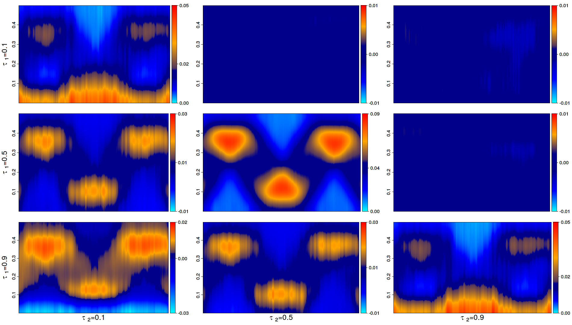
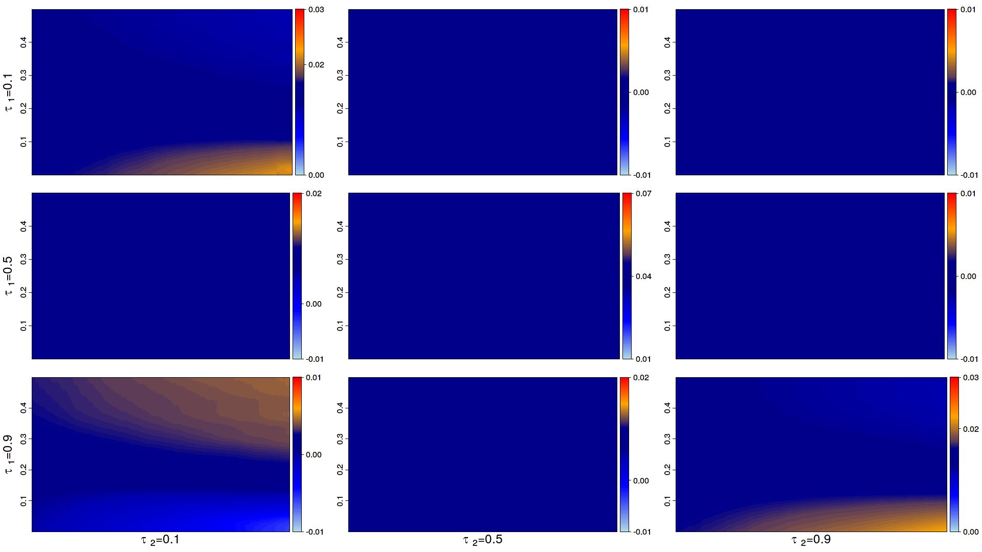
A.2.1 Gaussian tvAR(2)

In Figure 12, we display, for a classical Gaussian time-varying AR(2) process, the same heat maps as we did in Section 4.2; in particular, part (a) was obtained along the same lines as described there.

(a) Actual copula spectral densities (simulated)

(b) Estimated copula spectral densities, $n=128$

(c) Estimated copula spectral densities, $n=256$

(d) Estimated copula spectral densities, $n=512$

(e) Estimated copula spectral densities, $n=1024$

(f) Estimated copula spectral densities, $n=2048$

Figure 12: Heatmaps of the Gaussian time-varying AR(2) process described in Section A.2.1 and the corresponding estimators, for various window lenghts.

The model equation, taken from Dahlhaus, (2012), is

$$X_{t,T}=1.8\cos(1.5-\cos(2\pi t/T))X_{t-1,T}-0.81X_{t-2,T}+Z_{t}\vspace{-1mm}$$ (A.2)

with i.i.d. noise $Z_{t}\sim\mathcal{N}(0,1)$. Its strictly stationary approximation, at $t_{0}=\vartheta T$, $0\leq\vartheta\leq 1$, is

$$X_{t}^{\vartheta}=1.8\cos(1.5-\cos(2\pi\vartheta))X_{t-1}^{\vartheta}-0.81X_{t-2}^{\vartheta}+\zeta_{t}\vspace{-1mm}$$ (A.3)

where $\zeta_{t}$ similarly is $\mathcal{N}(0,1)$ white noise. This tvAR(2) process exhibits a time-varying periodicity which is clearly visible in the heat diagrams associated with the real parts of its time-varying copula-based spectral densities, displayed in the lower triangular part of Figure 12(b). The uniformly dark blue imaginary parts in the upper triangular part are a consequence of the fact that those imaginary parts actually are zero, since Gaussian processes are time-reversible [see Proposition 2.1 in Dette et al., (2015)]. As expected, no additional information can be gained from observing different quantiles (all heatmaps in the lower-triangular parts of (a) are the same), since the (bivariate) distributions of the process are Gaussian and the change over time only affects the correlation of these conditional distributions. Because of this the (time-varying) bivariate distribution functions (and with them all quantiles) depend only on the (time-varying) correlations of the random variables, which are also fully captured by $L_{2}$ methods.

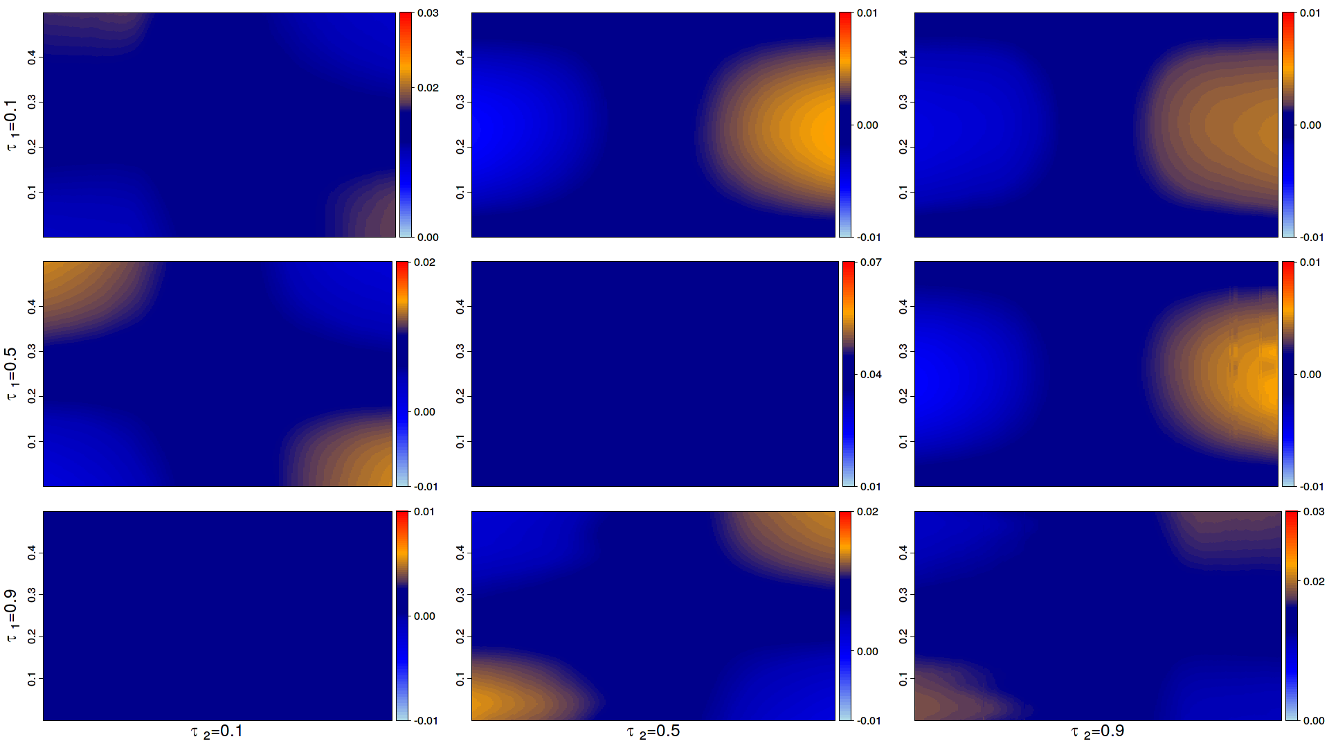
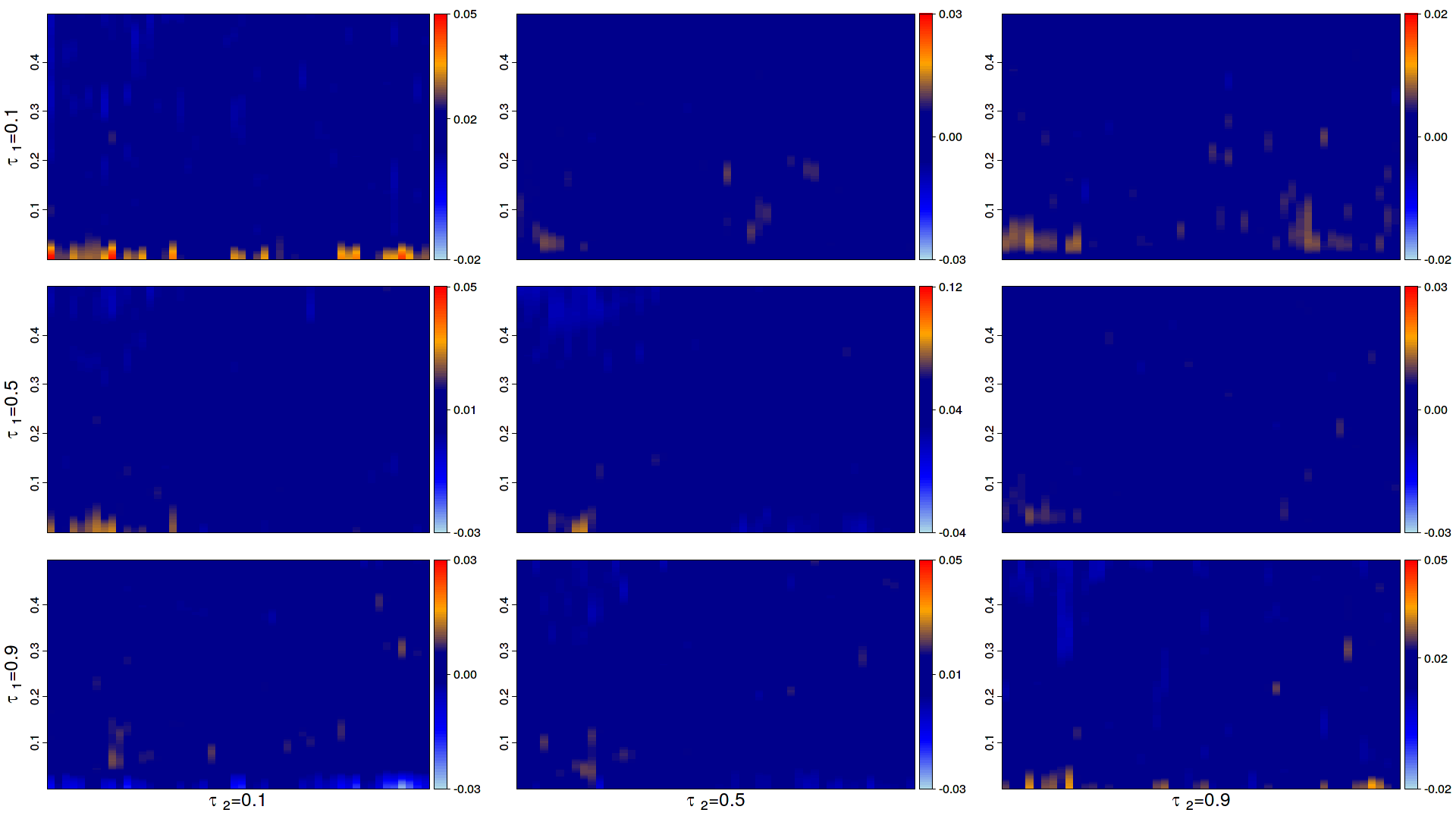
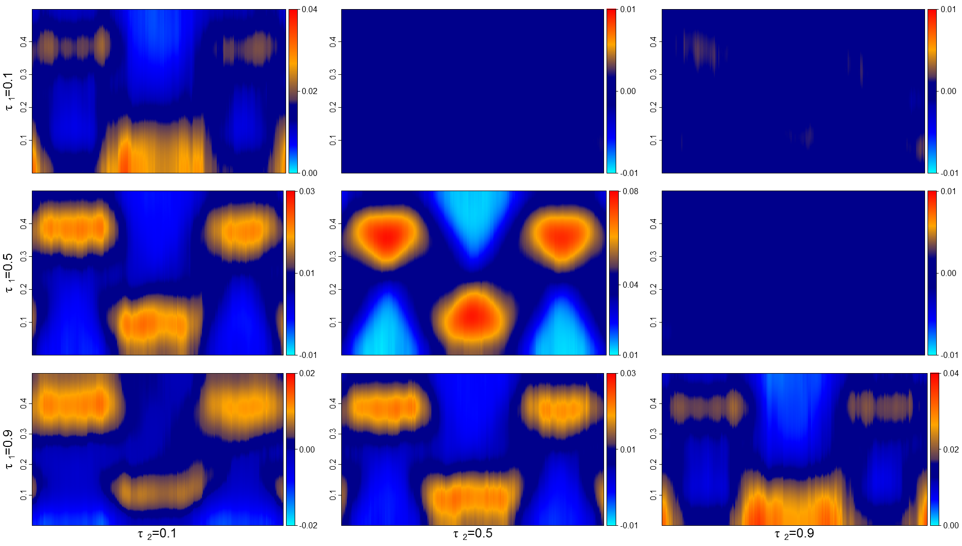
A.2.2 Gaussian tvARCH(1)

Figure 13 displays the same heatmaps for a time-varying ARCH(1) model of the form

$$X_{t,T}=\sqrt{1/2+(0.9t/T)X^{2}_{t-1,T}}Z_{t}\vspace{-1mm}$$

with i.i.d. noise $Z_{t}\sim\mathcal{N}(0,1)$ and its strictly stationary approximation at time $t_{0}=\vartheta T$, $0\leq\vartheta\leq 1$

$$X_{t}^{\vartheta}=\sqrt{1/2+0.9\vartheta(X_{t-1}^{\vartheta})^{2}}\zeta_{t}\vspace{-1mm}$$

where $\zeta_{t}$ similarly is $\mathcal{N}(0,1)$ white noise. In these stationary approximations, the influence of $X^{\vartheta}_{t-1}$ on the variance of $X^{\vartheta}_{t}$ gradually increases over time. This, quite understandably, gets reflected in the diagrams associated with extreme quantiles, but is not visible in the “median ones”.

(a) Actual copula spectral densities (simulated)

(b) Estimated copula spectral densities, $n=128$

(c) Estimated copula spectral densities, $n=256$

(d) Estimated copula spectral densities, $n=512$

(e) Estimated copula spectral densities, $n=1024$

(f) Estimated copula spectral densities, $n=2048$

Figure 13: Heatmaps of the Gaussian time-varying ARCH(1) process described in Section A.2.2 and the corresponding estimators, for various window lenghts.

A.2.3 Influence of the series length

As suggested by a referee we want to include heatmaps of estimators calculated from shorter time series $T$. In our non-stationary setting, a smaller $T$ is essentially equivalent to a faster evolution of the features of the process under study. Figure 14 compares estimators for the Cauchy tvAR$(2)$ and the tvQAR(1) processes (studied in Section 4.2.2) for series lengths $T=2^{12}=4096$ and $T=2^{11}=2048$ (one single realization), bandwidth $B_{n}=10$ and window length $w=512$. The results indicate that estimation rapidly deteriorates with decreasing $T$. While nonstationarity nevertheless remains quite significant in the Cauchy tvAR$(2)$ case, the signal in the real parts for the slowly varying tvQAR(1) is barely visible; time-irreversibility, on the other hand, remains well detected.

(a) Time-varying Cauchy AR$(2)$ with $T=4096$

(b) Time-varying Cauchy AR$(2)$ with $T=2048$

(c) Time-varying QAR$(1)$ with $T=4096$

(d) Time-varying QAR$(2)$ with $T=2048$

Figure 14: Heatmaps of estimated spectra for the time-varying Cauchy AR$(2)$ and QAR$(1)$ processes, $T=2^{12}=4096$ and $T=2^{11}=2048$.

A.3 Time-varying variances and low frequency peaks in quantile spectra

As mentioned in Section 4.3 and pointted out by Li, (2014), low frequency peaks in quantile spectral densities also can be caused by time-varying variances. By definition, copula spectra are invariant under strictly increasing transformations of the marginals. Invariance of the corresponding estimators, however, does not hold unless the pace of marginal changes is slow compared with the choice of local window lengths. Could fastly varying marginal variances, via some tvARCH model, account for the type of quantile spectral plots associated with the S&P500 data?

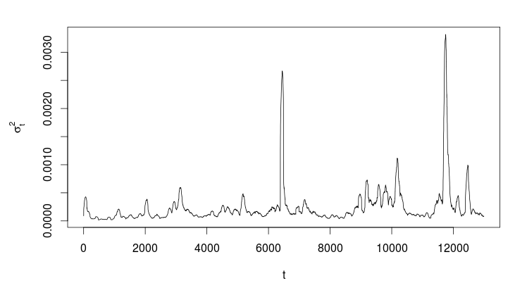
A.3.1 A tvARCH(0) model approach for S&P500 log-returns

A plot of the local variances of S&P500 returns (estimated in local windows) against time (Figure 16) suggests that those variances can be considered roughly stable over periods of at most 100 observations. This is quite small compared to the window length needed to estimate a quantile spectrum, a mismatch that could produce spurious deviations from white noise behavior in the heatmaps. To investigate whether such fast marginal changes can indeed produce the type of quantile spectral plots associated with the S&P500 data, we followed a heuristic approach inspired by Li, (2014). More precisely, based on local windows of length $101$ (details are provided in Section A.3.2), we first computed estimators $\hat{\sigma}^{2}_{t}$, $t=1,...,12992$, of the time-varying variances $\sigma^{2}_{t}$. With those estimated variances, we constructed an artificial series (of the tvARCH(0) form)

$$X_{t,T}=\hat{\sigma}_{t}Z_{t},$$ (A.4)

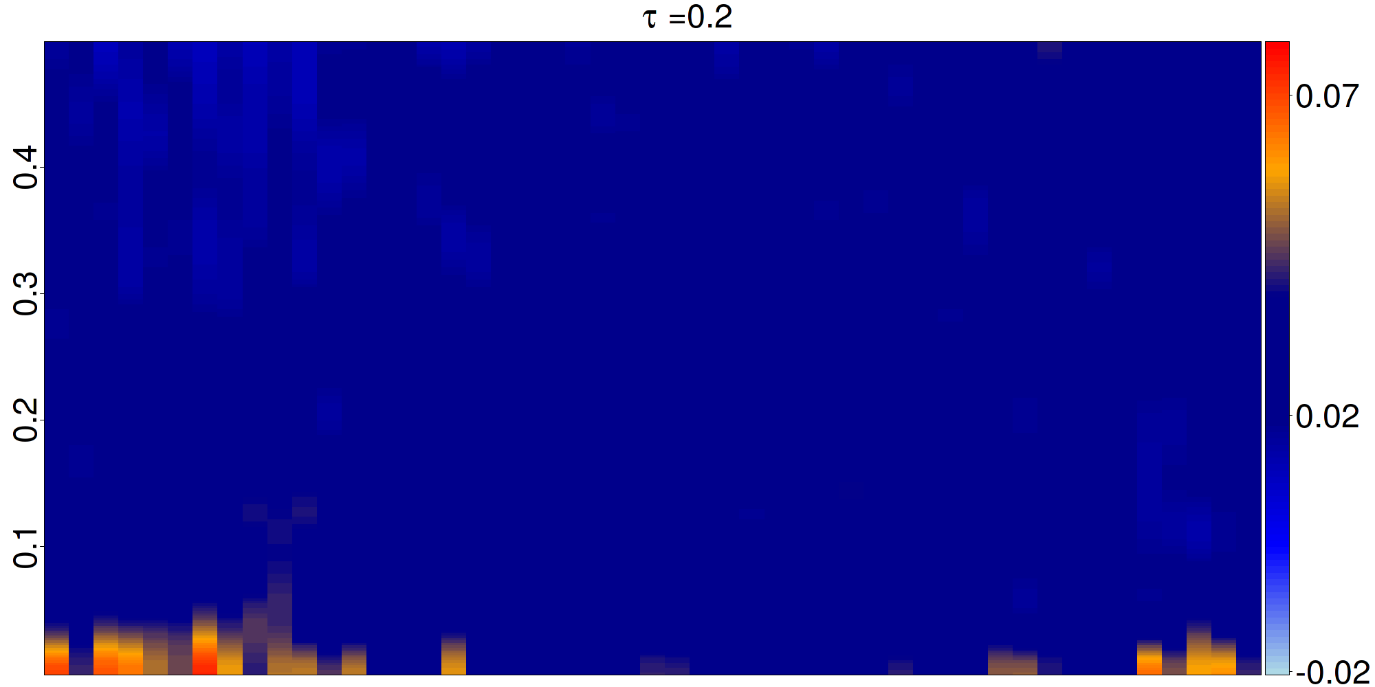
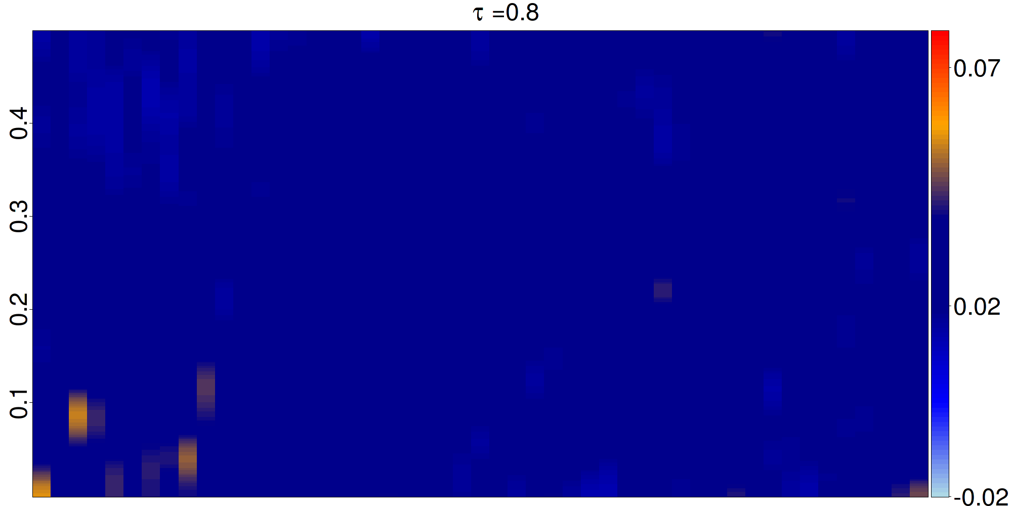
where $\{Z_{t}\}_{t=1}^{12992}$ denote i.i.d. draws with replacement from the S&P500 values $Y_{t}$ standardized by their estimated standard deviation, i.e. from $\{Y_{t}/\hat{\sigma}_{t}\}_{t=1}^{12992}$ where $(Y_{t})_{t=1}^{12992}$ denote the observed S&P500 returns. To see how well the time-varying copula spectrum of the S&P500 returns can be matched by the spectrum of the process $X_{t,T}$, we simulated $J=1000$ independent copies of $X_{t,T}$ and, for each realization, we computed local estimators of the quantile spectrum, $\hat{f}_{t_{0},T}^{j}$, say, $j=1,...,J$. Out of those $J=1000$ realizations, we selected one that produces quantile spectra matching those of the S&P500 return—see A.3.2 for details. For the sake of brevity, we restrict our comparison to the real parts of the quantile combinations $(\tau_{1},\tau_{2})\in\{(0.1,0.1),(0.9,0.9)\}$ and the imaginary parts corresponding to $(\tau_{1},\tau_{2})\in\{(0.1,0.9)\}$. The corresponding time-frequency plots are shown in Figure 15.

Figure 15: Time-frequency heatmaps for the S&P500 log-returns (left column) and one realization of a tvARCH(0) (right column) process where the parameter is estimated as the time-varying variance of the S&P500. First row: $\tau_{1}=\tau_{2}=0.1$. Second row: $\tau_{1}=\tau_{2}=0.9$. Third row: imaginary parts $(\tau_{1}=0.1,\tau_{2}=0.9)$.

Comparing the first two row figures corresponding to the quantile levels $(0.1,0.1)$ and $(0.9,0.9)$, we see that applying our estimators to the time-varying process $X_{t,T}$ indeed produces some peaks at low frequencies. However, those peaks, in the $(0.1,0.1)$-spectrum, are not enough, and not strong enough, thus failing to completely capture the strong dependence in negative returns which is one of the typical features of financial data. The imaginary parts of the $(0.1,0.9)$ S&P500 spectra (third row in Figure Figure 15) shows significant deviations from white noise behavior, in particular during the periods 1965–1973 and 1995–2003. In contrast to that, the corresponding imaginary parts for the time-varying process $X_{t,T}$ are virtually indistinguishable from those of a white noise spectrum. This indicates that a tvARCH(0) model does not provide an adequate description of the joint distributions of high and low returns and additional evidence that a tvARCH(0) model fails to capture important aspects of the S&P500 dynamics.

A.3.2 The “best  tvARCH$(0)$ fit” of the S&P500 data

Let us provide some details on the heuristic approach adopted in Section A.3.1. The time-varying variances $\sigma^{2}_{t}$ of the log-returns $Y_{1},\dots,Y_{T}$ were estimated by

$$\hat{\sigma}^{2}_{t}=\frac{1}{2n+1}\sum_{s=1}^{T}\bar{K}\big{(}\frac{s-t}{n}\big{)}\Big{(}Y_{t}-\frac{1}{2n+1}\sum_{|l-t|\leq n}Y_{l}\Big{)}^{2}$$

where $\bar{K}$ is the Parzen window multiplied with $4/3$ (so that it integrates to one), $n=50$ (accomodating fast changes that are still sufficiently smooth—see Figure 16). Note that, to compute $\hat{\sigma}^{2}_{t}$ for $t={1,\dots,12992},$ we need $13092$ observations of the S&P500 from 1962-01-02 to 2014-01-03. Those additional observations were omitted in the rest of the paper to keep all pictures consistent. For our investigation, we created $J=1000$ artificial time series as defined in $(\ref{eq:ARCH0})$ and for each of them, we calculated a collection of local lag-window estimators $\hat{f}_{t_{0},T}^{j}(\omega,\tau_{1},\tau_{2}),\ j=1,...,J$ by using the same windows and bandwidths as for the log-returns of the S&P500. To select the “best match”, we concentrate on the real parts of $\hat{f}_{t_{0},T}^{j}(\omega,0.1,0.1)$ and $\hat{f}_{t_{0},T}^{j}(\omega,0.9,0.9),$ and the imaginary part of $\hat{f}_{t_{0},T}^{j}(\omega,0.9,0.1).$ Let $\hat{f}_{t_{0},T}(\omega,\tau_{1},\tau_{2})$ stand for the local lag-window estimator of the S&P500 log-returns, and consider the $L^{2}$ distances

$$d_{1}(j)=\sum_{\omega\in\Omega}\sum_{t_{0}\in{\cal T}_{0}}[\Re\hat{f}_{t_{0},T}^{j}(\omega,0.1,0.1))-\Re\hat{f}_{t_{0},T}(\omega,0.1,0.1)]^{2},\qquad j=1,\dots,\ J.$$

Denote by $d_{2}(j)$ and $d_{3}(j)$ the same $L^{2}$ distances computed for the real and imaginary parts of $\hat{f}_{t_{0},T}^{j}(\omega,0.9,0.9)$ and $\hat{f}_{t_{0},T}^{j}(\omega,0.9,0.1)$ respectively. The “best match” was selected as the realization $j_{\text{min}}$ minimizing the sum $d_{1}(j)+d_{2}(j)+d_{3}(j).$

Figure 16: Estimated time-varying variance of the log-returns of the S&P500.

Figure 17: Log-returns of the S&P500 between 1963 and 2013 and the simulated tvARCH$(0)$ process that was selected as the “best match”.

A.3.3 Comparing the “global” tvARCH(0) and S&P500 spectra

If a tvARCH(0) approach to the study of the S&P500 data is to be adopted, one may argue that, in view the invariance argument mentioned at the beginning of this section, the localized spectral analysis developed in this paper is not required, and that the stationary or “global” methods developed in Dette et al., (2015) are the appropriate ones. The right check for the adequacy of a tvARCH(0) model then should be based on a comparison between (estimated) stationary quantile spectra, which avoids the trouble caused by a possible mismatch between the pace of marginal changes and the chosen window length.

Accordingly, in this section, we provide a comparison of the “global” spectra, i.e. spectra computed from the complete dataset, without localization, as in Dette et al., (2015), of the S&P500 returns on one hand, of the process $X_{t,T}$ defined in equation (A.4) on the other hand. We simulated $J=1000$ independent replications of the process $X_{t,T}$, and for each replication we computed the “global” lag-window estimator based on $\mathcal{N}_{t_{0},T}~{}:=~{}\{1,\dots,T\}$, the bandwidth $B_{n}=25$ and the same lag-window function as in the analysis of the S&P500 log returns. This yields a collection of estimators $(\hat{f}^{j})_{j=1,...,J}$. Next, for each frequency $\omega$ in $\{\frac{2\pi j}{6496}|j=0,\dots,6495\}$ and each couple $\tau_{1},\tau_{2}$ in $\{0.1,0.5,0.9\},$ we computed the $1\%$ quantile $q_{\text{min}}^{\Re}(\omega,\tau_{1},\tau_{2})$ of the $J$-tuple $(\Re\hat{f}^{j}(\omega,\tau_{1},\tau_{2}))_{j=1,...,J}$ and the $99\%$ quantile $q_{\text{max}}^{\Re}(\omega,\tau_{1},\tau_{2})$ of the $J$-tuple $(\Re\hat{f}^{j}(\omega,\tau_{1},\tau_{2}))_{j=1,...,J}$. The quantiles $q_{\text{max}}^{\Im}(\omega,\tau_{1},\tau_{2})$ and $q_{\text{max}}^{\Im}(\omega,\tau_{1},\tau_{2})$ were computed similarly.

Figure 18: A comparison of global lag-window estimations of the quantile spectra of the S&P500 (over the period 1962-2013; black lines) and those obtained from simulated tvARCH$(0)$ processes (red lines, with grey-shaded pointwise confidence regions).

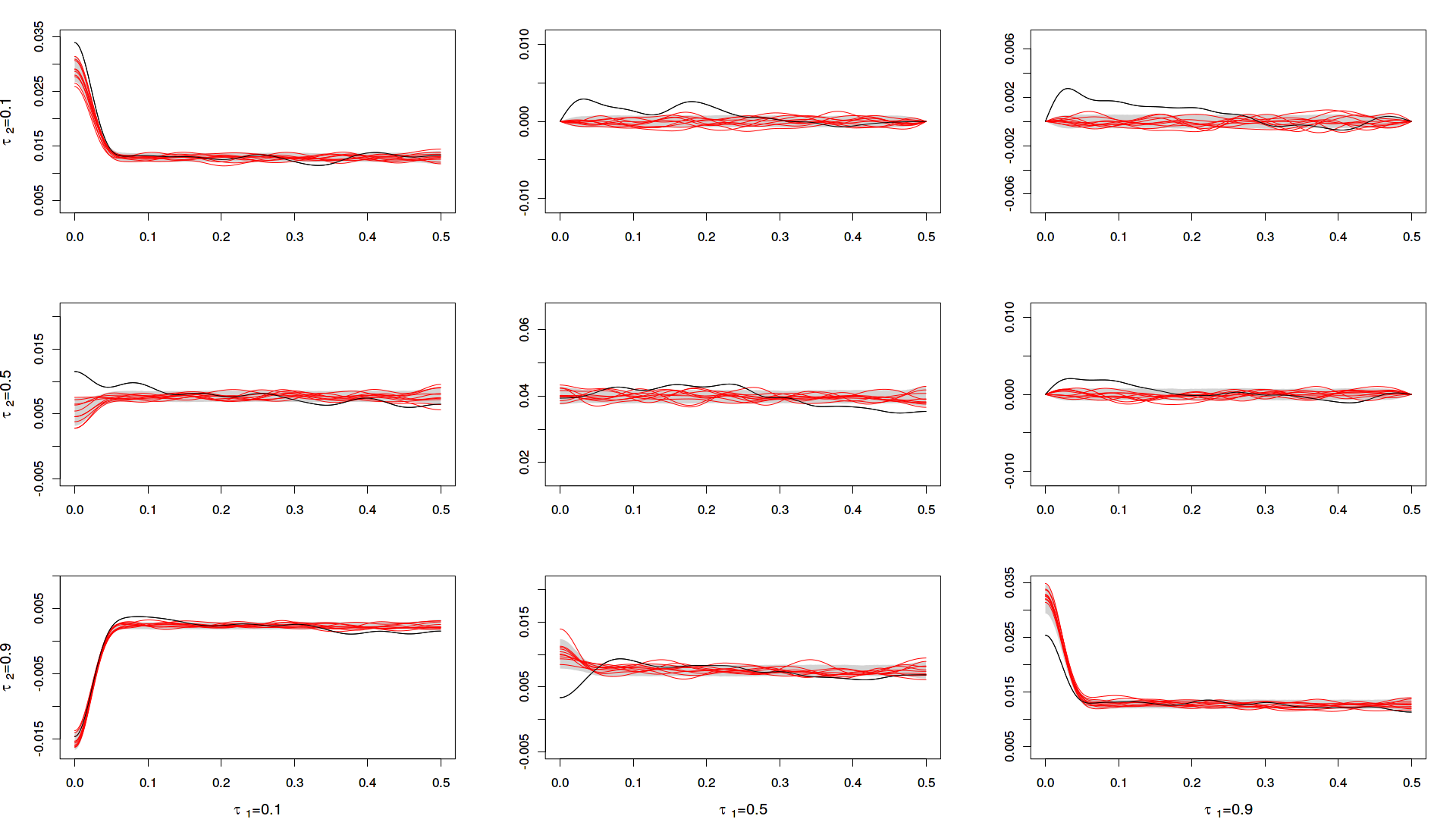
Quantile spectra computed from the S&P500 dataset (in black) are depicted in Figure 18, together with the estimators $\hat{f}^{j}(\omega,\tau_{1},\tau_{2}),\ j=1,...,10$ (red lines) and, for each $(\omega,\tau_{1},\tau_{2})$, a gray area covering the interval $[q_{\text{min}},q_{\text{max}}].$ As predicted by the analysis of Li, (2014), the $\tau_{1}=\tau_{2}=0.1$ and $\tau_{1}=\tau_{2}=0.9$ quantile spectral densities of the tvARCH(0) process exhibit prominent peaks around frequency zero. Observe, however, that those peaks are typically higher than those of the S&P500 for $\tau_{1}=\tau_{2}=0.1$ and (slightly) lower for $\tau_{1}=\tau_{2}=0.9$. Additionally, the estimators $\Re\hat{f}(\omega,\tau_{1},\tau_{2})$ for $(\tau_{1},\tau_{2})=(0.1,0.5)$, and $(0.9,0.5)$ and $\Im\hat{f}(\omega,\tau_{1},\tau_{2})$ for $(\tau_{1},\tau_{2})=(0.1,0.5),(0.1,0.9)$ and $(0.5,0.9)$ lie well outside the gray “confidence” areas for a wide range of frequencies. This again indicates that the tvARCH(0) process does not provide an adequate description of the (global) dynamic features of the S&P500 returns.

Figure 19: Same as Figure 18, with S&P500 observations restricted to the period 2000-2013.

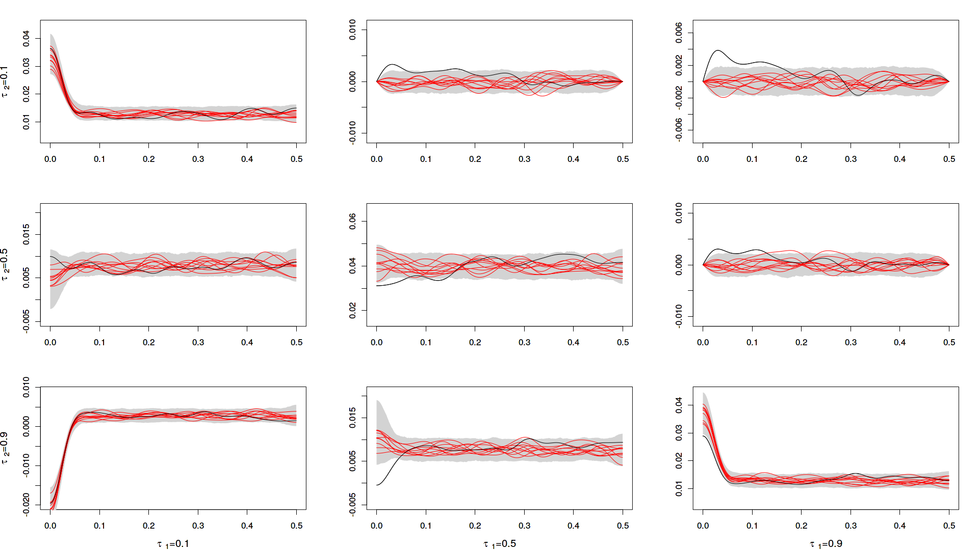
It is natural to wonder whether the mismatch between this simple time-varying variance model and the S&P500 data is due to a structural difference between the S&P500 dynamics back in the seventies and its more recent dynamics. To address this question, we replicated the procedure described above for the S&P500 returns in the time period 2000-2013. The corresponding results are displayed in Figure 19. While the estimators of the $(0.1,0.1)$ and $(0.9,0.9)$ spectra now (just barely) lie within the gray “confidence” areas, we still observe highly significant deviations between the imaginary part of the ARCH(0) and S&P500 spectra for the quantile combination $(\tau_{1},\tau_{2})=(0.1,0.9)$, and between their real parts for $(\tau_{1},\tau_{2})=(0.5,0.9)$.

Summarizing our findings, a localized analysis of quantile spectra reveals features that cannot be explained by a model based solely on fast local changes in variance. Note that more sophisticated models such as time-varying ARCH and GARCH processes have been suggested to describe financial data, see Fryzlewicz and Subba Rao, (2014) for a recent contribution. It would be very interesting to compare the quantile spectra of such time-varying stochastic volatility processes with those of the S&P500 returns. Preliminary comparisons indicate that the structure of the imaginary parts of the S&P500 time series cannot be explained by time-varying GARCH models.

A.4 Proofs for the main results

A.4.1 Proofs of the results in Section 5.1

We begin by some preliminary comments. Assume that $X_{t,T}$ and $X^{\vartheta}_{t}$ are defined on the same probability space. Expressing distributions function in terms of expectations and indicators leads to

$$|F_{t_{1},t_{2};T}(x_{1},x_{2})-G_{t_{2}-t_{1}}^{\vartheta}((x_{1},x_{2}))|$$

$$\quad=|\mathbb{E}(\prod_{1\leq j\leq 2}\mathbb{I}_{\{X_{t_{j},T}\leq x_{j}\}}-\prod_{1\leq j\leq p}\mathbb{I}_{\{(X^{\vartheta}_{t_{j}})\leq x_{j}\}})|$$

$$\quad\leq\sum_{k=1}^{2}|\mathbb{E}(\prod_{j=1}^{k-1}\mathbb{I}_{\{X_{t_{j},T}\leq x_{j}\}}[\mathbb{I}_{\{X_{t_{k},T}\leq x_{k}\}}-\mathbb{I}_{\{(X^{\vartheta}_{t_{k}})\leq x_{k}\}}]\prod_{j=k+1}^{p}\mathbb{I}_{\{(X^{\vartheta}_{t_{j}})\leq x_{j}\}})|$$

$$\quad\leq\sum_{k=1}^{2}\mathbb{E}(|\mathbb{I}_{\{X_{t_{k},T}\leq x_{j}\}}-\mathbb{I}_{\{(X^{\vartheta}_{t_{k}})\leq x_{j}\}}|).$$

Therefore, in order to prove Lemma 5.1-5.3, it is sufficent to show that

$$\sup_{x\in\mathbb{R}}\mathbb{E}(|\mathbb{I}_{\{X_{t,T}\leq x\}}-\mathbb{I}_{\{(X^{\vartheta}_{t})\leq x\}}|)\leq L\big{(}\big{|}\frac{t}{T}-\vartheta\big{|}+\frac{1}{T}\big{)}.$$

A.4.1.1 Proof of Lemma 5.1

By Assumption $(MA1)$, we have $\sup_{\vartheta\in(0,1)}\sum_{j=-\infty}^{\infty}|a(\vartheta,j)|<\infty$, which by standard arguments implies strict stationarity of the process $X^{\vartheta}_{t}$ (see for example Proposition $3.1.1$ in Brockwell and Davis, (1998)). Without loss of generality, we can assume that $\mu(\vartheta)=0$. In order to establish distributional properties, we always can specialize the noise $\zeta_{t}$ driving $X^{\vartheta}_{t}$–an arbitrary copy of the noise $Z_{t}$ driving $X_{t,T}$—as being $Z_{t}$ itself. Denoting by $\mathcal{A}$ the $\sigma-$field generated by $\{\xi_{s}|s\neq 0\},$

$$\sup_{x\in\mathbb{R}}\mathbb{E}(|\mathbb{I}_{\{X_{t,T}\leq x\}}-\mathbb{I}_{\{(X^{\vartheta}_{t})\leq x\}}|)$$

$$\qquad\leq\sup_{x\in\mathbb{R}}\mathbb{E}\big{[}\mathbb{E}(|\mathbb{I}_{\{X_{t,T}\leq x\}}-\mathbb{I}_{\{X^{\vartheta}_{t}\leq x\}}|\big{|}\mathcal{A})\big{]}$$

$$\qquad\leq\sup_{x\in\mathbb{R}}\mathbb{E}\big{[}\mathbb{E}(|\mathbb{I}_{\{\xi_{t}\leq\frac{1}{a_{t,T}(0)}\{x-\sum_{j\neq 0}a_{t,T}(j)\xi_{t-j}\}\}}-\mathbb{I}_{\{\xi_{t}\leq\frac{1}{a(\vartheta,0)}\{x-\sum_{j\neq 0}a(\vartheta,j)\xi_{t-j}\}\}}|\big{|}\mathcal{A})\big{]}$$

$$\qquad=\sup_{x\in\mathbb{R}}\mathbb{E}[|F_{\xi}(\frac{1}{a_{t,T}(0)}\{x-\sum_{j\neq 0}a_{t,T}(j)\xi_{t-j}\})-F_{\xi}(\frac{1}{a(\vartheta,0)}\{x-\sum_{j\neq 0}a(\vartheta,j)\xi_{t-j}\})|]$$

$$\qquad\leq\mathbb{E}[C_{1}|{a_{t,T}(0)}-{a(\vartheta,0)}|+C_{2}||S_{t,T}-S_{t}^{\vartheta}|],$$

where

$$S_{t,T}:=\sum_{j\neq 0}a_{t,T}(j)\xi_{t-j},\quad S_{t}^{\vartheta}:=\sum_{j\neq 0}a(\vartheta,j)\xi_{t-j},$$

and the last inequality follows from the two dimensional mean-value theorem. To be more precise,

$$\Big{|}F_{\xi}\left(\frac{x-v}{u}\right)-F_{\xi}\left(\frac{x-v^{\prime}}{u^{\prime}}\right)\Big{|}\\ \leq\Big{|}\int_{0}^{1}f_{\xi}\left(\frac{x-v_{t}}{u_{t}}\right)\frac{x-v_{t}}{u^{2}_{t}}dt\Big{|}|u-u^{\prime}|+\Big{|}\int_{0}^{1}f_{\xi}\left(\frac{x-v_{t}}{u_{t}}\right)\frac{1}{u_{t}}dt\Big{|}|v-v^{\prime}|,$$

with $u_{t}=u+t(u^{\prime}-u)$ and $v_{t}=v+t(v^{\prime}-v).$ From Assumption (MA2) the integrals are bounded by constants $C_{1}$ and $C_{2}$ which are independent of $x.$ Straightforward calculations, under the assumptions made, lead to

$$\mathbb{E}[|S_{t,T}-S_{t}^{\vartheta}|]=\text{O}(|t-\vartheta T^{-1}|+T^{-1}),$$

which completes the proof. ∎

A.4.1.2 Proof of Lemma 5.2

Observe that Assumptions (ARCH1) imply that

$$\sup_{\vartheta\in(0,1)}\mathbb{E}(\sum_{j=1}^{\infty}a_{j}(\vartheta)Z^{2}_{j})<1,$$ (A.5)

which is sufficient for the existence and uniqueness of a strictly stationary solution $(X^{\vartheta}_{t})^{2}$ with finite first moment(see Giraitis et al., (2000) Theorem $2.1$). Now $(ARCH1)$ yields $\sum_{j}|a_{j}(\vartheta)|<\infty,$ which implies that $(\sigma_{t}^{\vartheta})^{2}$ is locally strictly stationary (Proposition $3.1.1$ of Brockwell and Davis, (1998) again). Let $\sigma_{t}^{\vartheta}=\sqrt{(\sigma_{t}^{\vartheta})^{2}}$ and set $X^{\vartheta}_{t}=\sigma^{\vartheta}_{t}Z_{t}.$ To prove local strict stationarity, it suffices to bound $\sup_{x\in\mathbb{R}}\mathbb{E}(|\mathbb{I}_{\{X_{t,T}\leq x\}}-\mathbb{I}_{\{X^{\vartheta}_{t}\leq x\}}|).$ Denoting by $\mathcal{A}_{t}$ the $\sigma-$algebra generated by $(Z_{t},Z_{t-1},\dots),$ observe that

$$\mathbb{E}\big{(}\big{|}\mathbb{I}_{\{X_{t,T}\leq x\}}-\mathbb{I}_{\{X^{\vartheta}_{t}\leq x\}}\big{|}\big{)} =\mathbb{E}\big{(}\mathbb{E}\big{[}\big{|}\mathbb{I}_{\{X_{t,T}\leq x\}}-\mathbb{I}_{\{X^{\vartheta}_{t}\leq x\}}\big{|}\Big{|}\mathcal{A}_{t-1}\big{]}\big{)}$$

$$=\mathbb{E}\big{(}\mathbb{E}\big{[}\big{|}\mathbb{I}_{\{Z_{t}\leq x/\sigma_{t,T}\}}-\mathbb{I}_{\{Z_{t}\leq x/\sigma^{\vartheta}_{t}\}}\big{|}\Big{|}\mathcal{A}_{t-1}\big{]}\big{)} \leq\mathbb{E}\big{(}\big{|}F({x}/{\sigma_{t,T}})-F({x}/{\sigma^{\vartheta}})\big{|}\big{)}$$

$$=\mathbb{E}\big{(}\big{|}\int_{\sigma_{t,T}}^{\sigma^{\vartheta}_{t}}{x}{y}^{-1}f({x}{y}^{-1})y^{-1}dy\big{|}\big{)} \leq\mathbb{E}\big{(}C\big{|}{\sigma_{t,T}}-{\sigma^{\vartheta}_{t}}\big{|}\big{)},$$

where the last inequality follows from $(ARCH2)$ and the fact that $\min({\sigma_{t,T}},{\sigma^{\vartheta}_{t}})>\rho.$ Now, as $Z_{t}$ is independent of $(\sigma_{t,T},\sigma^{\vartheta}_{t}),$ we have

$$\mathbb{E}(|\sigma_{t,T}^{2}-(\sigma_{t}^{\vartheta})^{2}|)=\mathbb{E}[Z_{t}^{2}(|\sigma_{t,T}^{2}-(\sigma_{t}^{\vartheta})^{2}|)]=\mathbb{E}(|X_{t,T}^{2}-(X_{t}^{\vartheta})^{2}|)\leq\leq C\Big{(}\big{|}\frac{t}{T}-\vartheta\big{|}+\frac{1}{T}\Big{)}$$

where the last inequality follows from Theorem 1 in Dahlhaus and Subba Rao, (2006). Noting again that $\min({\sigma_{t,T}},{\sigma^{\vartheta}_{t}})$ is bounded away from zero, we have, for some appropriate constant $C$, $\mathbb{E}(|{\sigma_{t,T}}-{\sigma^{\vartheta}_{t}}|)\leq C\mathbb{E}(|{\sigma^{2}_{t,T}}-{(\sigma^{\vartheta}_{t})^{2}}|),$which concludes the proof. ∎

A.4.1.3 Proof of Lemma 5.3

Assumption $(GARCH1)$ implies that $\sup_{u\in[0,1]}\mathbb{E}(Z^{2}_{t})\Big{[}\sum_{j=1}^{p}a_{j}(u)+\sum_{i=1}^{q}b_{j}(u)\Big{]}<1$, which is sufficent for the existence of a strictly stationary solution $X^{\vartheta}_{t}$ (see the Remark after Corollary 2.2 in Bougerol and Picard, (1992)). Similar calculations as in the tvARCH case yield $\mathbb{E}(|\mathbb{I}_{\{X_{t,T}\leq x\}}-\mathbb{I}_{\{X^{\vartheta}_{t}\leq x\}}|)\leq\mathbb{E}(C|{\sigma^{2}_{t,T}}-{(\sigma^{\vartheta}_{t}})^{2})$, and a bound on $\mathbb{E}(|{\sigma^{2}_{t,T}}-{(\sigma^{\vartheta}_{t})^{2}}|)$ follows as in Section $5.2.$ (top of page $1168$) of Subba Rao, (2006). ∎

A.4.2 Proof of Theorem 5.1

The proof proceeds in several steps, which we briefly outline here; details are provided in Section A.6. First, we establish that the estimator $\hat{q}_{t_{0},T}(\tau)$ can be replaced with the true quantile levels $\tau$, that is,

$$\hat{\mathfrak{f}}_{t_{0},T}(\omega_{n},\tau_{1},\tau_{2})=\frac{1}{2\pi}\sum_{|k|\leq n-1}K_{n}(k)e^{-i\omega_{n}k}$$

$$\qquad\times\frac{1}{n}\sum_{t\in T(k)}\Big{(}\mathbb{I}_{\{X_{t,T}\leq q^{\vartheta}(\tau_{1})\}}-\tau_{1}\Big{)}\Big{(}\mathbb{I}_{\{X_{t+k,T}\leq q^{\vartheta}(\tau_{2})\}}-\tau_{2}\Big{)}+o_{P}((B_{n}/n)^{1/2}),$$ (A.6)

uniformly in $\omega_{n}\in\tilde{\mathcal{F}}_{n}(\varepsilon),$ where $\tilde{\mathcal{F}}_{n}(\varepsilon)$ denotes the set of all Fourier frequencies in the interval $(\varepsilon,\pi-\varepsilon)$. Second, we prove that, uniformly again in $\omega_{n}\in\tilde{\mathcal{F}}_{n}(\varepsilon)$,

$$\hat{\mathfrak{f}}_{t_{0},T}(\omega_{n},\tau_{1},\tau_{2})=\tilde{\mathfrak{f}}_{t_{0},T}(\omega_{n},\tau_{1},\tau_{2})+O_{P}\Big{(}\frac{B_{n}^{2}}{n}+\frac{n^{2}}{T^{2}B_{n}}+\frac{n^{1/2}B_{n}}{T}\Big{)}$$ (A.7)

where

$$\tilde{\mathfrak{f}}_{t_{0},T}(\omega_{n},\tau_{1},\tau_{2}):=\frac{1}{2\pi}\frac{1}{n}\sum_{|k|\leq n-1}K_{n}(k)e^{-i\omega_{n}k}\sum_{|t-t_{0}|\leq m_{T}-B_{n}}Y_{t,\tau_{1}}Y_{t+k,\tau_{2}}$$

and $Y_{t,\tau}:=\mathbb{I}_{\{X_{t,T}\leq q^{\vartheta}(\tau)\}}-F_{t;T}(q^{\vartheta}(\tau))$. The advantage of this representation lies in the fact that the random variables $\mathbb{I}_{\{X_{t,T}\leq q^{\vartheta}(\tau_{1})\}}-F_{t;T}(q^{\vartheta}(\tau_{1}))$ are centered, which considerably simplifies some of the computations that follow. Next, observe that

$$\tilde{\mathfrak{f}}_{t_{0},T}(\omega_{n},\tau_{1},\tau_{2})=\tilde{\mathfrak{f}}_{t_{0},T}(\omega,\tau_{1},\tau_{2})+O_{P}(B_{n}/n)$$

since $|\omega_{n}-\omega|=O(1/n)$. Finally, we prove that

$$\sqrt{B_{n}/n}\left(\begin{array}[]{c}\Re\tilde{\mathfrak{f}}_{t_{0},T}(\omega,\tau_{1},\tau_{2})-\Re\mathbb{E}\tilde{\mathfrak{f}}_{t_{0},T}(\omega,\tau_{1},\tau_{2})\\ \Im\tilde{\mathfrak{f}}_{t_{0},T}(\omega,\tau_{1},\tau_{2})-\Im\mathbb{E}\tilde{\mathfrak{f}}_{t_{0},T}(\omega,\tau_{1},\tau_{2})\end{array}\right)\stackrel{{\scriptstyle\mathcal{D}}}{{\longrightarrow}}\mathcal{N}(0,\Sigma^{2}(\omega,\tau_{1},\tau_{2}))$$ (A.8)

and

$$\mathbb{E}\tilde{\mathfrak{f}}_{t_{0},T}(\omega,\tau_{1},\tau_{2})= \mathfrak{f}^{\vartheta}(\omega,\tau_{1},\tau_{2})-C_{K}(r)B_{n}^{-r}\mathfrak{d}^{(r)}_{\omega}\mathfrak{f}^{\vartheta}(\omega,\tau_{1},\tau_{2})$$

$$\qquad+\frac{n^{2}}{2T^{2}}\frac{\partial^{2}}{\partial u^{2}}\mathfrak{f}^{u}(\omega,G^{u}(q^{\vartheta}(\tau_{1})),G^{u}(q^{\vartheta}(\tau_{2})))\Big{|}_{u=\vartheta}$$ (A.9)

$$\qquad+o(B_{n}^{-r}+n^{2}/T^{2})+O(1/n),$$

which completes the proof of the theorem. ∎

A.5 Some probabilistic details

A.5.1 A Lemma on cumulants

Lemma A.5.1.

For an arbitrary stochastic process $(X_{t})_{t\in\mathbb{Z}}$, let

$$\alpha(n):=\sup_{t\in\mathbb{Z}}\sup_{A\in\sigma(..X_{t-1},X_{t}),B\in\sigma(X_{t+n},X_{t+n+1},...)}|\mathbb{P}(A\cap B)-\mathbb{P}(A)\mathbb{P}(B)|.$$

Then, for any $t_{1},...,t_{p}\in\mathbb{Z}$ and any p-tuple Borel sets $A_{1},...,A_{p}$ there exists a constant $K_{p}$ depending on $p$ only such that

$$\Big{|}\mathrm{cum}(I\{X_{t_{1}}\in A_{1}\},\ldots,I\{X_{t_{p}}\in A_{p}\})\Big{|}\leq K_{p}\alpha\Big{(}\big{\lfloor}p^{-1}\max_{i,j}|t_{i}-t_{j}|\big{\rfloor}\Big{)}.$$

Proof. Recall that, by the definition of cumulants,

$$|\mathrm{cum}(I\{X_{t_{1}}\in A_{1}\},\ldots,I\{X_{t_{p}}\in A_{p}\})|$$

$$=\Big{|}\sum_{\{\nu_{1},\ldots,\nu_{R}\}}(-1)^{R-1}(R-1)!\mathbb{P}\Big{(}\bigcap_{i\in\nu_{1}}\{X_{t_{i}}\in A_{i}\}\Big{)}\cdots\mathbb{P}\Big{(}\bigcap_{i\in\nu_{R}}\{X_{t_{i}}\in A_{i}\}\Big{)}\Big{|},$$ (A.10)

where the summation runs over all partitions $\{\nu_{1},\ldots,\nu_{R}\}$ of the set $\{1,\ldots,p\}$. In the case $t_{1}=...=t_{p},$ the Lemma is obviously true. If at least two indices are distinct, choose $j$ with $\max_{i=1,\ldots,p-1}(t_{i+1}-t_{i})=t_{j+1}-t_{j}>0$ and let $(Y_{t_{j+1}},\ldots,Y_{t_{p}})$ be a random vector that is independent of $(X_{t_{1}},\ldots,X_{t_{j}})$ and possesses the same joint distribution as $(X_{t_{j+1}},\ldots,X_{t_{p}})$. By an elementary property of the cumulants (cf. Theorem 2.3.1 (iii) in Brillinger, (1975)), we have

$$\mathrm{cum}\big{(}I\{X_{t_{1}}\in A_{1}\},\ldots,I\{X_{t_{j}}\in A_{j}\},I\{Y_{t_{j+1}}\in A_{j+1}\},\ldots,I\{Y_{t_{p}}\in A_{p}\}\big{)}=0.$$

Therefore, we can write, for the cumulant of interest,

$$\begin{split}&\Big{|}\mathrm{cum}(I\{X_{t_{1}}\in A_{1}\},\ldots,I\{X_{t_{p}}\in A_{p}\})\\ &\quad-\mathrm{cum}(I\{X_{t_{1}}\in A_{1}\},\ldots,I\{X_{t_{j}}\in A_{j}\},I\{Y_{t_{j+1}}\in A_{j+1}\},\ldots,I\{Y_{t_{p}}\in A_{p}\})\Big{|}\\ &=\Big{|}\!\!\sum_{\{\nu_{1},\ldots,\nu_{R}\}}(-1)^{R-1}(R-1)![P_{\nu_{1}}\cdots P_{\nu_{R}}-Q_{\nu_{1}}\cdots Q_{\nu_{R}}]\Big{|},\end{split}$$

where the sum again runs over all partitions $\{\nu_{1},\ldots,\nu_{R}\}$ of $\{1,\ldots,p\}$,

$$P_{\nu_{r}}\!:=\mathbb{P}\Big{(}\bigcap_{i\in\nu_{r}}\{X_{t_{i}}\in A_{i}\}\Big{)}\ \text{ and }\ Q_{\nu_{r}}\!:=\mathbb{P}\Big{(}\bigcap_{\begin{subarray}{c}i\in\nu_{r}\\ i\leq j\end{subarray}}\{X_{t_{i}}\in A_{i}\}\Big{)}\mathbb{P}\Big{(}\bigcap_{\begin{subarray}{c}i\in\nu_{r}\\ i>j\end{subarray}}\{X_{t_{i}}\in A_{i}\}\Big{)},$$

$r=1,\ldots,R$, with $\mathbb{P}(\bigcap_{i\in\emptyset}\{X_{t_{i}}\in A_{i}\}):=1$ by convention. By the definition of $\alpha(n)$, it follows that $|P_{\nu_{r}}-Q_{\nu_{r}}|\leq\alpha(t_{j+1}-t_{j})$ for any partition $\nu_{1},...,\nu_{R}$ and any $r=1,...,R$. Thus, for every partition $\nu_{1},...,\nu_{R}$,

$$|P_{\nu_{1}}\cdots P_{\nu_{R}}-Q_{\nu_{1}}\cdots Q_{\nu_{R}}|\leq\sum_{r=1}^{R}|P_{\nu_{r}}-Q_{\nu_{r}}|\leq R\alpha(t_{j+1}-t_{j}).$$

All together, this yields

$$|\mathrm{cum}(I\{X_{t_{1}}\in A_{1}\},\ldots,I\{X_{t_{p}}\in A_{p}\})|\leq\alpha(t_{j+1}-t_{j})\sum_{\{\nu_{1},\ldots,\nu_{R}\}}R!\ .$$

Noting that $p(t_{j+1}-t_{j})\geq\max_{i_{1},i_{2}}|t_{i_{1}}-t_{i_{2}}|$ and observing that $\alpha$ is a monotone function, we obtain

$$|\mathrm{cum}(I\{X_{t_{1}}\in A_{1}\},\ldots,I\{X_{t_{p}}\in A_{p}\})|\leq K_{p}\alpha(\max|t_{i}-t_{j}|).\vspace{-10mm}$$

∎

Lemma A.5.2.

Let $F$ and $G$ denote functions on the real line, with $|G(x)-G(y)|>c|x-y|$ for $x,y\in[a,b]$ where $c$ is some positive constant. For all $p,q\in(a,b),$ with $F(p)=G(q)$ and any $\epsilon>0,$ $||F(\cdot)-G(\cdot)||_{\infty}\leq\epsilon$ implies $|p-q|\leq{\epsilon}/{c}.$

Proof. The claim follows from the fact that

$$c|p-q|<|G(p)-G(q)|=|G(p)-F(p)|\leq\epsilon.\vspace{-12mm}$$

∎

A.5.2 A blocking technique for nonstationary $\beta$-mixing processes

In her paper, Yu, (1994) constructed an independent block (IB) technique to transfer the classical tools from the i.i.d. case to the case of $\beta$-mixing stationary time series. We are using the same technique here to derive results for sums of $\beta$-mixing local stationary time series, which will be used on multiple occasions. For this purpose, let $X_{t,n}$ be a triangular array of $\beta$-mixing processes with mixing coefficient $\beta_{n}$. For each fixed $n$ we will divide the process $X_{t,n}$ into $2\mu_{n}$ alternating blocks with lengths $p_{n}$ and $q_{n},$ respectively, and a remainder block of length $n-2\mu_{n}(p_{n}+q_{n}).$ More precisely, we divide the index set into $(2\mu_{n}+1)$ parts

$$\Gamma_{j}=\{t:t_{\text{min}}+B_{n}+(j-1)(p_{n}+q_{n})+1\leq t\leq t_{\text{min}}+B_{n}+(j-1)(p_{n}+q_{n})+p_{n}\}$$

$$\Delta_{j}=\{t:t_{\text{min}}+B_{n}+(j-1)(p_{n}+q_{n})+p_{n}+1\leq t\leq t_{\text{min}}+B_{n}+j(p_{n}+q_{n})\}$$

$$R=\{t:t_{\text{min}}+B_{n}+\mu_{n}(p_{n}+q_{n})+1\leq t\leq t_{\text{min}}+n-B_{n}\},$$

and introduce the notation

$$X(\Gamma_{j})=\{X_{i,n},i\in\Gamma_{j}\},\quad X(\Delta_{j})=\{X_{i,n},i\in\Delta_{j}\}\quad\text{and}\quad X(R)=\{X_{i,n},i\in R\},$$

where the dependence on $n$ is omitted for the sake of brevity. We now have a sequence of alternating $X(\Gamma_{j})$ and $X(\Delta_{j})$ blocks, and a remainder block $X(R):$

$$X=X(\Gamma_{1}),X(\Delta_{1}),X(\Gamma_{2}),\dots,X(\Gamma_{\mu_{n}}),X(\Delta_{\mu_{n}}),X(R).$$

To exploit the concept of coupling, we consider a one-dependent block sequence

$$Y=Y(\Gamma_{1}),Y(\Delta_{1}),Y(\Gamma_{2}),\dots,Y(\Gamma_{\mu_{n}}),Y(\Delta_{\mu_{n}}),$$

where $Y(\Gamma_{j})=\{\xi_{i}:i\in\Gamma_{j}\}$ and $Y(\Delta_{j})=\{Y_{i}:i\in\Delta_{j}\}$ such that the sequence is independent of $X$ and each block of $Y$ has the same distribution as the corresponding block in $X$, that is,

$$Y(\Gamma_{i})\overset{d}{=}X(\Gamma_{i})\quad\text{and}\quad Y(\Delta_{i})\overset{d}{=}X(\Delta_{i}),$$

where $\overset{d}{=}$ stands for equality in distribution.

The existence of such a sequence and the measurability issues that arise are addressed in Yu, (1994). The $\Gamma$- and $\Delta$-block subsequences are denoted by $X_{\Gamma},Y_{\Gamma},X_{\Delta}$ and $Y_{\Delta}$, respectively: for instance,

$$X_{\Gamma}:=X(\Gamma_{1}),X(\Gamma_{2}),\dots,X(\Gamma_{\mu_{n}}).$$

We obtain $X_{\Gamma}$ by leaving out every other block in the original sequence, which is $\beta$-mixing, so that the dependence between the blocks in $X_{\Gamma}$ becomes weaker as the size $p_{n}$ of the $\Gamma$-blocks increases. The following lemma from Yu, (1994) establishes an upper bound for the difference between the $\Gamma$-block sequences from the original process and the independent block sequence.

Lemma A.5.3.

For any measurable function $h$ on $\mathbb{R}^{\mu_{n}q_{n}}$ with $\|h\|_{\infty}\leq M,$ we have, for the blocking structure just described,

$$\Big{|}\mathbb{E}_{Q}[h(X(\Delta))]-\mathbb{E}_{\tilde{Q}}[h(Y(\Delta))]\Big{|} \leq M(\mu_{n}-1)\beta_{p_{n}}\quad\text{and}$$

$$\Big{|}\mathbb{E}_{Q}[h(X(\Gamma))]-\mathbb{E}_{\tilde{Q}}[h(Y(\Gamma))]\Big{|} \leq M(\mu_{n}-1)\beta_{q_{n}}.$$

Proof.

We only prove the first claim, which follows as an application of Corollary 2.7 in Yu, (1994) with $Q$ being the probability distribution of the $\Delta_{j}$ block sequence. However, note that the $\beta$-mixing rate of $Q$ here is less than $\beta_{p_{n}},$ due to the alternating block length. ∎

Next, we consider a special case of the same blocking technique with $a_{n}:=q_{n}=p_{n},$ now applied to a sum of $\beta$-mixing random variables, namely $\sum_{t=1}^{n}f(X_{t,n}),$ and link its probabilistic behavior to that of the sum of the independent blocks $\sum_{j=1}^{\mu_{n}}\sum_{i\in\Gamma_{j}}f(Y_{i,n}).$ To avoid measurability issues the function $f$ is assumed to belong to a permissable class $F_{n}$ of functions (for a definition see the appendix in Yu, (1994)). Furthermore, for the sake of simplicity, assume that $\mathbb{E}(f(X_{i,n}))=0$ for all $f\in F_{n}.$ The following Lemma is a slight adjustment of Lemma $4.2$ from Yu, (1994).

Lemma A.5.4.

Let $F_{n}$ be a sequence of permissible function classes, which are bounded by a constant $M_{n}$. If a sequence $(r_{n})_{n\in\mathbb{N}}$ is such that, for $n$ large enough, $2r_{n}\mu_{n}\geq nM_{n},$ we have

$$\mathbb{P}\Big{(}\sup_{f\in F_{n}}\big{|}\sum_{t=1}^{n}f(X_{t,n})\big{|}>4r_{n}\Big{)} \leq\mathbb{P}\Big{(}\sup_{f\in F_{n}}\big{|}\sum_{j=1}^{\mu_{n}}\sum_{i\in\Gamma_{j}}f(Y_{i,n})\big{|}>r_{n}\Big{)}$$ (A.11)

$$\quad+\mathbb{P}\Big{(}\sup_{f\in F_{n}}\big{|}\sum_{j=1}^{\mu_{n}}\sum_{i\in\Delta_{j}}f(Y_{i,n})\big{|}>r_{n}\Big{)}+2\mu_{n}\beta_{a_{n}}.$$

Proof. The probability in the left-hand side of $(\ref{eqn:lem6.7})$ splits into three parts: namely,

$$\mathbb{P}\Big{(}\sup_{f\in F_{n}}\big{|}\sum_{t=1}^{n}f(X_{t,n})\big{|}>4r_{n}\Big{)} \leq\mathbb{P}\Big{(}\sup_{f\in F_{n}}\big{|}\sum_{j=1}^{\mu_{n}}\sum_{i\in\Gamma_{j}}f(X_{i,n})\big{|}>r_{n}\Big{)}$$

$$\quad+\mathbb{P}\Big{(}\sup_{f\in F_{n}}\big{|}\sum_{j=1}^{\mu_{n}}\sum_{i\in\Delta_{j}}f(X_{i,n})\big{|}>r_{n}\Big{)}$$

$$\quad+\mathbb{P}\Big{(}\sup_{f\in F_{n}}\big{|}\sum_{i\in R}f(X_{i,n})\big{|}>2r_{n}\Big{)}.$$

The sum appearing in the third part, which deals with the ramainder block, is bounded by $M_{n}(2a_{n})\leq M_{n}n/\mu_{n}.$ As $2r_{n}\mu_{n}\geq nM_{n},$ that probability is zero.

Turning to the first part, Lemma A.5.3 with $h$ the indicator function of the event

$$\Big{\{}\sup_{f\in F_{n}}\big{|}\sum_{j=1}^{\mu_{n}}\sum_{i\in\Gamma_{j}}f(X_{i,n})\big{|}>r_{n}\Big{\}}$$

yields

$$\mathbb{P}\Big{(}\sup_{f\in F_{n}}\big{|}\sum_{j=1}^{\mu_{n}}\sum_{i\in\Gamma_{j}}f(X_{i,n})\big{|}>r_{n}\Big{)}\leq\mathbb{P}\Big{(}\sup_{f\in F_{n}}\big{|}\sum_{j=1}^{\mu_{n}}\sum_{i\in\Gamma_{j}}f(Y_{i,n})\big{|}>r_{n}\Big{)}+\mu_{n}\beta_{a_{n}},$$

the second term can be treated by the same arguments. The claim follows. ∎

The upper bound in Lemma A.5.4 is based on i.i.d. blocks, which allows us to use classical techniques. In particular, we will apply the Benett inequality to further bound the sum of $\beta$-mixing random variables. For this purpose assume that the number of functions $m_{f}(n)$ contained in $F_{n}$ is finite, so that

$$\mathbb{P}\Big{(}\sup_{f\in F_{n}}\big{|}\sum_{j=1}^{\mu_{n}}\sum_{i\in\Gamma_{j}}f(Y_{i,n})\big{|}\Big{)}\leq m_{f}(n)\sup_{f\in F_{n}}\mathbb{P}\Big{(}\big{|}\sum_{j=1}^{\mu_{n}}\sum_{i\in\Gamma_{j}}f(Y_{i,n})\big{|}>r_{n}\Big{)}.$$

Furthermore, let us assume that the variance $\mathrm{Var}(\sum_{j=1}^{\mu_{n}}\sum_{i\in\Gamma_{j}}f(Y_{i,n}))$ of the blocks is bounded by some finite $V_{n}$, so that the Benett inequality yields

$$\mathbb{P}\Big{(}\big{|}\sum_{j=1}^{\mu_{n}}\sum_{i\in\Gamma_{j}}f(Y_{i,n})\big{|}>r_{n}\Big{)}\leq\exp\Big{(}-\frac{\mu_{n}V_{n}}{a_{n}^{2}M_{n}^{2}}h\Big{(}\frac{r_{n}a_{n}M_{n}}{2\mu_{n}V_{n}}\Big{)}\Big{)},$$ (A.12)

where $h(x)=(1+x)log(1+x).$ Calculations similar to those in the proof of Lemma 6.7 in Dette et al., (2015) we can bound the probability by

$$\exp\Big{(}-\frac{\log 2}{2}\Big{(}\frac{r_{n}^{2}}{4\mu_{n}V_{n}}\wedge\frac{r_{n}}{2a_{n}M_{n}}\Big{)}\Big{)}.$$

We just have proven the following Lemma

Lemma A.5.5.

Let $X_{t,n}$ be a triangular array of $\beta$-mixing random variables and $F_{n}$ a sequence of finite function classes with cardinality $\#F_{n}$ that fulfills

$$(i)\#F_{n}\leq m_{f}(n),\quad(ii)\sup_{f\in F_{n}}|f(X_{t,n})|\leq M_{n}\quad\text{and}\quad(iii)~{}\mathbb{E}(f(X))=0$$

Assume a blocking structure with block length $a_{n}:=p_{n}=q_{n}$ which divides the index set into $2\mu_{n}+1$ parts, where $n/2-a_{n}\leq\mu_{n}a_{n}\leq n/2,\ a_{n}\rightarrow\infty$ and $\mu_{n}\rightarrow\infty$, satisfying

1. $\mu_{n}\beta_{a_{n}}\xrightarrow{n\rightarrow\infty}0,$

2. $2r_{n}\mu_{n}\geq nM_{n}$ and

3. $\mathrm{Var}(\sum_{i\in\Gamma_{j}}f(X_{i,n}))\vee\mathrm{Var}(\sum_{i\in\Delta_{j}}f(X_{i,n}))\leq V_{n}$ for all $1\leq j\leq\mu_{n}.$

If these conditions are met ,we obtain

$$\mathbb{P}\Big{(}\sup_{f\in F_{n}}\big{|}\sum_{t=1}^{n}f(X_{t,n})\big{|}>4r_{n}\Big{)}\leq 2m_{f}(n)\exp\Big{(}-\frac{\log 2}{2}\Big{(}\frac{r_{n}^{2}}{4\mu_{n}V_{n}}\wedge\frac{r_{n}}{2a_{n}M_{n}}\Big{)}\Big{)}+o(1).$$

A.5.3 Auxiliary technical results

Lemma A.5.6.

Assume that $M_{T}\to\infty,\ T/M_{T}\to 0\text{ and }t_{0}/T\to\vartheta\in(0,1)$. Under Assumptions (A1)-(A4), for any bounded $S\subset\mathbb{R},$

$$\Big{(}\sqrt{2M_{T}}\Big{(}\frac{1}{2M_{T}}\sum_{|t-t_{0}|\leq M_{T}}(I\{X_{t,T}\leq x\}-F_{t,T}(x))\Big{)}\Big{)}_{x\in\mathbb{R}}\stackrel{{\scriptstyle\mathcal{D}}}{{\longrightarrow}}\mathbb{B}\quad\mbox{in}\quad\ell^{\infty}(S)$$

where $\mathbb{B}$ denotes a centered Gaussian process with covariances

$$\mathbb{E}[\mathbb{B}(s)\mathbb{B}(t)]=\sum_{k\in\mathbb{Z}}\big{(}G^{\vartheta}_{k}(x,y)-G^{\vartheta}(x)G^{\vartheta}(y)\big{)}.$$

Proof. In order to prove weak convergence, we need to establish asymptotic equicontinuity and convergence of finite-dimensional distributions (see Theorem 2.1 in Kosorok, (2007)). Convergence of finite-dimensional distributions follows as an application of Lemma A.5.3 the arguments are quite standard and omitted for the sake of brevity. To prove asymptotic equicontinuity, we apply Lemma 7.1 from Kley et al., (2016). More precisely, consider the process $H_{n}(x):=\frac{1}{\sqrt{2M_{T}}}\sum_{|t-t_{0}|\leq M_{T}}(I\{X_{t,T}\leq x\}-F_{t,T}(x)),$ where $n$ denotes the cardinality of the set $\{t\in\{1,\dots,T\}:|t-t_{0}|\leq M_{T}\}$. Then,

$$H_{n}(x)-H_{n}(y)=\sum_{|t-t_{0}|\leq M_{T}}W_{t,T}(x,y)$$

where

$$W_{t,T}(x,y):=\frac{1}{\sqrt{2M_{T}}}\Big{(}I\{X_{t,T}\leq x\}-F_{t,T}(x)-(I\{X_{t,T}\leq y\}-F_{t,T}(y)))\Big{)}.$$

Since $\mathbb{E}W_{t,T}(x,y)=0$ for all $x,y$, by the definition of cumulants, we have

$$\mathbb{E}|H_{n}(x)-H_{n}(y)|^{4}=3\Big{(}\mathrm{cum}_{2}\Big{(}\sum_{|t-t_{0}|\leq M_{T}}W_{t,T}(x,y)\Big{)}\Big{)}^{2}+\mathrm{cum}_{4}\Big{(}\sum_{|t-t_{0}|\leq M_{T}}W_{t,T}(x,y)\Big{)}$$

where $\mathrm{cum}_{k}(y):=\mathrm{cum}(y,...,y)$. Assumption (A3)(iii) implies that

$$\mathrm{cum}_{4}\Big{(}\sum_{|t-t_{0}|\leq M_{T}}W_{t,T}(x,y)\Big{)}=O(1/M_{T})$$

while, under Assumption (A3)(i), there exist constants $C$ and $\tilde{C}$ such that

$$\Big{|}\mathrm{cum}_{2}\Big{(}\sum_{|t-t_{0}|\leq M_{T}}W_{t,T}(x,y)\Big{)}\Big{|}\leq|x-y|+C\sum_{s\geq 1}\min(|x-y|,s|^{\gamma})\leq\tilde{C}|x-y|^{1-\gamma^{-1}}$$

where the last equality follows by (A.22). Thus, there exists a constant $C>0$ such that, for $|x-y|\geq 1/M_{T}^{1/2}$, we have

$$\mathbb{E}|H_{n}(x)-H_{n}(y)|^{4}\leq C|x-y|^{2-2\gamma^{-1}}.$$

Now, fix $\delta>0$ and apply Lemma 7.1 from Dette et al., (2015) with

$$\Psi(x)=x^{4},\quad d(x,y):=|x-y|^{(\gamma-1)/(2\gamma)},\quad\bar{\eta}:=(2/n)^{(\gamma-1)/(2\gamma)},\quad\mathbb{G}_{x}:=H_{n}(x),\quad\!\text{and}\quad\!T:=S.$$

In particular, the packing number of the bounded set $S$ with respect to the metric $d$ can be bounded by $D(\varepsilon,d)\leq C\varepsilon^{-2\gamma/(\gamma-1)}$ for some constant $C$ independent of $\varepsilon$. This yields

$$\sup_{x,y\in S,d(x,y)\leq\delta}|H_{n}(x)-H_{n}(y)|\leq S_{1}+2\sup_{x,y\in S,d(x,y)\leq\bar{\eta}}|H_{n}(x)-H_{n}(y)|$$ (A.13)

where the quantity $S_{1}$ satisfies

$$\|\mathbb{E}S_{1}^{4}\|^{1/4}\leq K\Big{[}\int_{\bar{\eta}/2}^{\eta}\varepsilon^{-\gamma/2(\gamma-1)}d\varepsilon+(\delta+2\bar{\eta})\eta^{-\gamma/(\gamma-1)}\Big{]}.$$ (A.14)

Note that $\gamma>2$ implies $\gamma/2(\gamma-1)<1,$ so that $\varepsilon^{-\gamma/2(\gamma-1)}$ is integrable on $[0,1]$. In particular, setting $\eta:=\delta^{(\gamma-1)/(2\gamma)}$ implies $\delta\eta^{-\gamma/(\gamma-1)}=\delta^{1/2},$ hence

$$\lim_{\delta\downarrow 0}\limsup_{n\to\infty}\|\mathbb{E}S_{1}^{4}\|^{1/4}=0.$$

Finally, note that similar arguments as in the proof of (A.6.1) entail

$$\sup_{x,y\in S,d(x,y)\leq\bar{\eta}}|H_{n}(x)-H_{n}(y)|=o_{P}(1).$$ (A.15)

Jointly, (A.13)-(A.15) imply that, for any $\alpha>0,$

$$\lim_{\delta\downarrow 0}\limsup_{n\to\infty}P\Big{(}\sup_{x,y\in S,d(x,y)\leq\delta}|H_{n}(x)-H_{n}(y)|\geq\alpha\Big{)}=0.$$

Since the metric $d$ makes the index set $S$ totally bounded, condition (ii) in Theorem 2.1 in Kosorok, (2007) follows. This, together with the weak convergence of the finite-dimensional distributions, completes the proof. ∎

Lemma A.5.7.

Let $\ell_{n}\in\mathbb{Z}$ be a sequence such that $\omega_{\ell_{n}}:=2\pi\ell_{n}/n\rightarrow\omega\not\equiv 0\mod 2\pi$. Let $K$ be a function satisfying assumption (K) and define $K_{n}(k):=K(k/B_{n})$, for $k\in\mathbb{Z}$, where $B_{n}=o(n)$. Denote by $\tilde{\mathcal{F}}_{n}(\varepsilon)$ the set of Fourier frequencies which are contained in $(\varepsilon,\pi-\varepsilon)$. Assume that condition (A4)(iv) holds. Then

$$\sup_{\omega\in\tilde{\mathcal{F}}_{n}(\varepsilon)}\sup_{t\in\mathcal{N}_{t_{0},T}}\sup_{\tau}\Big{|}\sum_{|k|\leq B_{n}}K_{n}(k){\rm e}^{-{\rm i}\omega k}\big{(}F_{t+k;T}(q^{\vartheta}(\tau))-\tau\big{)}\Big{|}=O\Big{(}\frac{n}{TB_{n}^{d-1}}+B_{n}/T\Big{)}$$

and

$$\sup_{\omega\in\tilde{\mathcal{F}}_{n}(\varepsilon)}\Big{|}\sum_{|k|\leq B_{n}}K_{n}(k){\rm e}^{-{\rm i}\omega k}\Big{|}=O\Big{(}\frac{1}{B_{n}^{d-1}}\Big{)}.$$

Proof. We only establish the first statement since the second one can be proved by similar arguments. Let $h_{t,T}(u):=K\big{(}u\frac{n}{B_{n}}\big{)}[G^{\frac{t}{T}+u\frac{n}{T}}(q^{\vartheta}(\tau))-\tau]$, $u\in[-1/2,1/2]$ for $T$ large enough that $|un/B_{n}|\leq 1$ and $\frac{k}{T}+u\frac{n}{T}\in[0,1]$. Note that, under the assumptions made, this function has support $[-B_{n}/n,B_{n}/n]$ and is $d$ times continuously differentiable as a function on $(-1/2,1/2)$. Due to local stationarity the following approximation holds:

$$\begin{split}&\sum_{|k|\leq B_{n}}K\Big{(}\frac{k}{B_{n}}\Big{)}{\rm e}^{-{\rm i}\omega k}[F_{t+k;T}(q^{\vartheta}(\tau))-\tau]\\ &\qquad=\sum_{k=-n/2+1}^{n/2}K\Big{(}\frac{k}{n}\frac{n}{B_{n}}\Big{)}[G^{\frac{t}{T}+\frac{k}{n}\frac{n}{T}}(q^{\vartheta}(\tau))-\tau]{\rm e}^{-{\rm i}\omega k}+O(B_{n}/T)\\ &\qquad=\sum_{k=-n/2+1}^{n/2}h_{t,T}(k/n){\rm e}^{-{\rm i}\omega k}+O(B_{n}/T).\end{split}$$

By Leibniz’s rule, we have

$$\begin{split}h^{(d)}_{t,T}(u)&=\sum_{j=0}^{d-1}\binom{d}{j}\Big{(}\frac{n}{B_{n}}\Big{)}^{j}\Big{(}\frac{n}{T}\Big{)}^{d-j}K^{(j)}\Big{(}u\frac{n}{B_{n}}\Big{)}\frac{\partial^{d-j}}{\partial v^{d-j}}G^{\frac{t}{T}+v}(q^{\vartheta}(\tau))\Big{|}_{v=u\frac{n}{T}},\\ &\quad+\Big{(}\frac{n}{B_{n}}\Big{)}^{d}K^{(d)}\Big{(}u\frac{n}{B_{n}}\Big{)}\Big{(}G^{\frac{t}{T}+u\frac{n}{T}}(q^{\vartheta}(\tau))-\tau\Big{)}\end{split}$$

so that, under the assumptions made, for some constant $C_{d}$ depending only on $K$, $d$, and the mapping $u\mapsto G^{u}(q_{\tau}),$

$$\sup_{t,T,u}|h^{(d)}_{t,T}(u)|\leq C_{d}(n/B_{n})^{d}\frac{n}{T}.$$

Note that, under the assumptions of the lemma, the function $u\mapsto h_{t,T}(u)$ is twice continuously differentiable on $(-1/2,1/2)$. Thus, it admits the Fourier series representation

$$h_{t,T}(u)=\sum_{j\in\mathbb{Z}}c_{j,t,T}{\rm e}^{{\rm i}2\pi ju},\quad\text{where }c_{j,t,T}:=\int_{-1/2}^{1/2}h_{t,T}(u){\rm e}^{-{\rm i}2\pi ju}{\rm d}u.$$

Now consider a Fourier frequency $\omega_{\ell}=2\pi\ell/n\in\tilde{\mathcal{F}}_{n}(\varepsilon)$. By the usual argument (see Briggs and Henson, (1995), page 182), we have the discrete Poisson summation formula

$$\sum_{k=-n/2+1}^{n/2}h_{t,T}(k/n){\rm e}^{-{\rm i}\omega_{\ell}k} =\sum_{j\in\mathbb{Z}}c_{j,t,T}\sum_{k=-n/2+1}^{n/2}{\rm e}^{{\rm i}2\pi k(j-\ell)/n}$$

$$=n\Big{(}c_{\ell,t,T}+\sum_{k=1}^{\infty}(c_{\ell+kn,t,T}+c_{\ell-kn,t,T})\Big{)}.$$

For the leading term, note that $h^{(r)}_{t,T}(u)=0$ for $|u|>B_{n}/n$, so that, integrating by parts yields

$$c_{\ell,t,T}=(-1)^{d+1}\frac{1}{({\rm i}2\pi\ell)^{d}}\int_{-B_{n}/n}^{B_{n}/n}h^{(d)}_{t,T}(u){\rm e}^{-{\rm i}2\pi\ell u}{\rm d}u.$$ (A.16)

It follows that $|c_{\ell,t,T}|\leq 2C_{p}(2\pi\ell)^{-d}\frac{n}{T}(n/B_{n})^{d-1}\lesssim\frac{1}{TB_{n}^{d-1}}$, as $\ell\asymp n$. Furthermore, by Assumption (A4)(iv) (recall that $d\geq 2$ and $\ell/n\to c\in(0,1)\text{ mod }1$),

$$\begin{split}\Big{|}\sum_{k=1}^{\infty}(c_{\ell+kn,t,T}+c_{\ell-kn,t,T})\Big{|}&\lesssim\frac{n}{T}\Big{(}\frac{n}{B_{n}}\Big{)}^{d-1}\sum_{k=1}^{\infty}\Big{(}\frac{1}{(\ell+kn)^{d}}+\frac{1}{(\ell-kn)^{d}}\Big{)}\\ &=\frac{1}{TB_{n}^{d-1}}\sum_{k=1}^{\infty}\Big{(}\frac{1}{(\ell/n+k)^{d}}+\frac{1}{(\ell/n-k)^{d}}\Big{)}\lesssim\frac{1}{TB_{n}^{d-1}}.\end{split}$$

Note that all the bounds above hold uniformly in $\ell\asymp n$. This completes the proof of the lemma. ∎

A.6 Details for the proof of Theorem 5.1

A.6.1 Proof of (A.4.2)

Define

$$\hat{F}_{t_{0},t_{0}+k;T}(x,y):=\frac{1}{n}\sum_{t\in T(k)}\mathbb{I}_{\{X_{t,T}\leq x,X_{t+k,T}\leq y\}},$$

and let

$$r_{n,1}(k) := \hat{F}_{t_{0},t_{0}+k;T}(\hat{q}_{t_{0},T}(\tau_{1}),\hat{q}_{t_{0},T}(\tau_{2}))-\hat{F}_{t_{0},t_{0}+k;T}(q^{\vartheta}(\tau_{1}),q^{\vartheta}(\tau_{2}))$$

$$\quad\quad\quad-\frac{1}{n}\sum_{t\in T(k)}\Big{(}F_{t,t+k;T}(\hat{q}_{t_{0},T}(\tau_{1}),\hat{q}_{t_{0},T}(\tau_{2}))-F_{t,t+k;T}(q^{\vartheta}(\tau_{1}),q^{\vartheta}(\tau_{2}))\Big{)},$$

$$r_{n,2}(k) := \frac{1}{n}\sum_{t\in T(k)}\Big{[}F_{t,t+k;T}(\hat{q}_{t_{0},T}(\tau_{1}),\hat{q}_{t_{0},T}(\tau_{2}))-F_{t;T}(\hat{q}_{t_{0},T}(\tau_{1}))F_{t+k;T}(\hat{q}_{t_{0},T}(\tau_{2}))$$

$$\quad\quad\quad\quad\quad\quad\quad-\Big{(}F_{t,t+k;T}(q^{\vartheta}(\tau_{1}),q^{\vartheta}(\tau_{2}))-F_{t;T}(q^{\vartheta}(\tau_{1}))F_{t+k;T}(q^{\vartheta}(\tau_{2}))\Big{)}\Big{]},$$

$$r_{n,3}(k) := \frac{1}{n}\sum_{t\in T(k)}\Big{(}F_{t;T}(\hat{q}_{t_{0},T}(\tau_{1}))F_{t+k;T}(\hat{q}_{t_{0},T}(\tau_{2}))-F_{t;T}(q^{\vartheta}(\tau_{1}))F_{t+k;T}(q^{\vartheta}(\tau_{2}))\Big{)},$$

$$r_{n,4}(k) := \frac{\tau_{1}}{n}\sum_{t\in T(k)}\Big{(}\mathbb{I}_{\{X_{t+k,T}\leq\hat{q}_{t_{0},T}(\tau_{2})\}}-\tau_{2}\Big{)}+\frac{\tau_{2}}{n}\sum_{t\in T(k)}\Big{(}\mathbb{I}_{\{X_{t,T}\leq\hat{q}_{t_{0},T}(\tau_{1})\}}-\tau_{1}\Big{)}$$

$$-\frac{\tau_{1}}{n}\sum_{t\in T(k)}\Big{(}\mathbb{I}_{\{X_{t+k,T}\leq q^{\vartheta}(\tau_{2})\}}-\tau_{2}\Big{)}-\frac{\tau_{2}}{n}\sum_{t\in T(k)}\Big{(}\mathbb{I}_{\{X_{t,T}\leq q^{\vartheta}(\tau_{1})\}}-\tau_{1}\Big{)}.$$

Observe that, due to the assumptions on $K_{n},$

$$2\pi\hat{\mathfrak{f}}_{t_{0},T}(\omega,\tau_{1},\tau_{2})-\sum_{|k|\leq n-1}K_{n}(k)e^{-i\omega k}\frac{1}{n}\sum_{t\in T(k)}\Big{(}\mathbb{I}_{\{X_{t,T}\leq q^{\vartheta}(\tau_{1})\}}-\tau_{1}\Big{)}\Big{(}\mathbb{I}_{\{X_{t+k,T}\leq q^{\vartheta}(\tau_{2})\}}-\tau_{2}\Big{)}$$

$$\qquad=\sum_{|k|\leq B_{n}}K_{n}(k)e^{-i\omega k}\Big{(}r_{n,1}(k)+r_{n,2}(k)+r_{n,3}(k)+r_{n,4}(k)\Big{)}$$

$$\qquad=:R_{n,1}+R_{n,2}+R_{n,3}+R_{n,4},\text{ say.}$$

To prove (A.4.2) it is sufficient to establish the following statements:

$$\max(|q^{\vartheta}(\tau_{1})-\hat{q}_{t_{0},T}(\tau_{1})|,|q^{\vartheta}(\tau_{2})-\hat{q}_{t_{0},T}(\tau_{2})|)=O_{P}(T^{-2/5}),$$ (A.17)

$$\sup_{k}\sup_{x\in X}\sup_{\|y\|\leq\varepsilon_{n}} \Big{|}\hat{F}_{t_{0},t_{0}+k;T}(x)-\hat{F}_{t_{0},t_{0}+k;T}(x+y)-\frac{1}{n}\sum_{t\in T(k)}[F_{t,t+k;T}(x)-F_{t,t+k;T}(x+y)]\Big{|}$$

$$=O_{\mathbb{P}}(\rho_{n}(\varepsilon_{n})),$$ (A.18)

for any $\varepsilon_{n}=o(1)$ and any bounded set $X\subset\mathbb{R}^{2}$ with $\|v\|$ denoting the maximum norm of the vector $v$, and

$$\sup_{x\in Z}\sup_{|y|\leq\varepsilon_{n}}\Big{|}\frac{1}{n}\sum_{|t-t_{0}|\leq m_{T}}\Big{(}\mathbb{I}_{\{X_{t,T}\leq x\}}-\mathbb{I}_{\{X_{t,T}\leq x+y\}}-F_{t;T}(x)+F_{t;T}(x+y)\Big{)}\Big{|}=O_{\mathbb{P}}(\rho_{n}(\varepsilon_{n}))$$ (A.19)

for any $\varepsilon_{n}=o(1)$ and any bounded set $Z\subset\mathbb{R}$ where $\rho_{n}$ is defined in Assumption (A2). We first analyze the asymptotic behavior of the four remainder terms $R_{n,1},R_{n,2},R_{n,3},R_{n,4}$, then turn to the proofs for (A.17) - (A.19).

Discussion of remainder term $R_{n,1}$.
From (A.17) and (A.6.1), we obtain $\sup_{k}|r_{n,1}(k)|=O_{P}(\rho_{n}(T^{-2/5}))$ hence under (A3)

$$|R_{n,1}|=o_{P}(B_{n}^{1/2}n^{-1/2}).$$ (A.20)

Discussion of remainder term $R_{n,2}$.
Under (A3)(i) and (A4)(i), $|r_{n,2}(k)|=O(\min(|k|^{-\gamma},T^{-2/5})),$ and thus

$$|R_{n,2}|\leq\sum_{|k|\leq B_{n}}O(\min(|k|^{-\gamma},T^{-2/5}))=O(T^{-(1-\gamma^{-1})2/5})=o(B_{n}^{1/2}n^{-1/2}).$$ (A.21)

To see the this, note that, for $\varepsilon\to 0,$

$$\sum_{k\geq 1}\min(k^{-\gamma},\varepsilon)\leq\sum_{1\leq k\leq\varepsilon^{-1/\gamma}}\varepsilon+\sum_{k\geq\varepsilon^{-1/\gamma}}k^{-\gamma}=O(\varepsilon^{1-1/\gamma})+O(\varepsilon^{(-1/\gamma)(1-\gamma)})=O(\varepsilon^{1-\gamma^{-1}}).$$ (A.22)

Discussion of remainder term $R_{n,3}.$
Start by observing that

$$\frac{1}{n}\sum_{t\in T(k)}F_{t;T}(x)F_{t+k;T}(y) = \frac{1}{n}\sum_{|t-t_{0}|\leq m_{T}}F_{t;T}(x)F_{t+k;T}(y)+O(k/n)$$

$$= \frac{1}{n}\sum_{|t-t_{0}|\leq m_{T}}G^{t/T}(x)G^{(t+k)/T}(y)+O(k/n)+O(1/T)$$

$$= \frac{1}{n}\sum_{|t-t_{0}|\leq m_{T}}G^{t/T}(x)G^{t/T}(y)+O(k/T)+O(k/n)+O(1/T)$$

$$= \frac{T}{2m_{T}}\int_{-m_{T}/T}^{m_{T}/T}G^{\vartheta+u}(x)G^{\vartheta+u}(y)du+O(k/n),$$

where we have used a first-order Taylor expansion of the function $u\mapsto G^{u}(x)$. This yields

$$r_{n,3}(k)=\frac{T}{2m_{T}}\int_{-m_{T}/T}^{m_{T}/T} G^{\vartheta+u}(\hat{q}_{t_{0},T}(\tau_{1}))G^{\vartheta+u}(\hat{q}_{t_{0},T}(\tau_{2}))$$

$$\quad-G^{\vartheta+u}(q^{\vartheta}(\tau_{1}))G^{\vartheta+u}(q^{\vartheta}(\tau_{2}))du+O(B_{n}/n),$$

uniformly in $|k|\leq B_{n}$. Observe that, by Lemma A.5.7 under condition (K), we have

$$\sup_{\omega\in\tilde{\mathcal{F}}_{n}(\varepsilon)}\Big{|}\sum_{|k|\leq n-1}K_{n}(k)e^{-ik\omega}\Big{|}=O(1).$$

This implies

$$R_{n3}= \Big{(}\sum_{|k|\leq B_{n}}K_{n}(k)e^{-i\omega k}\Big{)}\frac{T}{2m_{T}}\int_{-m_{T}/T}^{m_{T}/T}G^{\vartheta+u}(\hat{q}_{t_{0},T}(\tau_{1}))G^{\vartheta+u}(\hat{q}_{t_{0},T}(\tau_{2}))$$

$$\hskip 142.26378pt-G^{\vartheta+u}(q^{\vartheta}(\tau_{1}))G^{\vartheta+u}(q^{\vartheta}(\tau_{2}))du+O(B_{n}^{2}/n)$$

$$= \ O\Big{(}\max\big{(}|q^{\vartheta}(\tau_{1})-\hat{q}_{t_{0},T}(\tau_{1})|,|q^{\vartheta}(\tau_{2})-\hat{q}_{t_{0},T}(\tau_{2})|\big{)}\Big{)}+O(B_{n}^{2}/n)$$

uniformly in $\omega\in\tilde{\mathcal{F}}_{n}(\varepsilon),$ almost surely. Recalling (A.17) and Assumption (A2) we thus obtain

$$|R_{n,3}|=o_{P}(B_{n}^{1/2}n^{-1/2}).$$ (A.23)

Discussion of remainder term $R_{n,4}.$
Observe that, uniformly in $|k|\leq B_{n}$ and $y\in\mathbb{R}$ we have

$$\frac{1}{n}\sum_{t\in T(k)}\mathbb{I}_{\{X_{t,T}\leq y\}}=\frac{1}{n}\sum_{|t-t_{0}|\leq m_{T}}\mathbb{I}_{\{X_{t,T}\leq y\}}+O_{P}(B_{n}/n),$$

$$\frac{1}{n}\sum_{t\in T(k)}\mathbb{I}_{\{X_{t+k,T}\leq y\}}=\frac{1}{n}\sum_{|t-t_{0}|\leq m_{T}}\mathbb{I}_{\{X_{t,T}\leq y\}}+O_{P}(B_{n}/n).$$

Thus, uniformly in $|k|\leq B_{n}$, $r_{n,4}(k)=D_{n}+O_{P}(B_{n}/n)$, where

$$D_{n}:=\sum_{|t-t_{0}|\leq m_{T}}\frac{\tau_{1}}{n}\Big{(}\mathbb{I}_{\{X_{t,T}\leq\hat{q}_{t_{0},T}(\tau_{2})\}}-\mathbb{I}_{\{X_{t,T}\leq q^{\vartheta}(\tau_{2})\}}\Big{)}+\frac{\tau_{2}}{n}\Big{(}\mathbb{I}_{\{X_{t,T}\leq\hat{q}_{t_{0},T}(\tau_{1})\}}-\mathbb{I}_{\{X_{t,T}\leq q^{\vartheta}(\tau_{1})\}}\Big{)}$$

does not depend on $k$. In particular, by Lemma A.5.7 this implies

$$|R_{n,4}|\leq O_{P}(B_{n}^{2}/n)+|D_{n}|\sup_{\omega\in\tilde{\mathcal{F}}_{n}(\varepsilon)}\Big{|}\sum_{|k|\leq n-1}K_{n}(k)e^{-ik\omega}\Big{|}=O_{P}(B_{n}^{2}/n)+|D_{n}|O(B_{n}^{-1}).$$

To conclude with $R_{n,4}$, note that combining (A.17), (A.19), and Assumption (A4)(i) we obtain $|D_{n}|=O_{P}(\rho_{n}(T^{-2/5}))+O_{P}(T^{-2/5})$. Together with (A2), this entails $R_{n,4}=o_{P}(B_{n}^{1/2}/n^{1/2})$ which, combined with (A.20)-(A.23), yields (A.4.2). It remains to establish (A.17) - (A.19).

Proof of (A.17) Letting $M_{T}=T^{4/5}$ in Lemma A.5.6, we obtain the weak convergence of $\sqrt{2T^{4/5}}(\tilde{F}_{t_{0};T}(x)-\bar{F}(x)),$ where

$$\bar{F}(x):=\frac{1}{2T^{4/5}}\sum_{|t-t_{0}|\leq T^{4/5}}F_{t;T}(x)=\frac{1}{2T^{4/5}}\sum_{|t-t_{0}|\leq T^{4/5}}G^{t/T}(x)+O(1/T).$$

to a centered Gaussian process with almost surely continuous sample paths. Next, observe that, uniformly in $x,$

$$\bar{F}(x)=\frac{T}{2T^{4/5}}\int_{-T^{4/5}/T}^{T^{4/5}/T}G^{\vartheta+u}(x)du+O(1/T)=G^{\vartheta}(x)+O((T^{4/5}/T)^{2})+O(1/T)$$

where we have used a second-order Taylor expansion of the function $u\mapsto G^{\vartheta+u}(x)$. The claim (statement (A.17)) follows by compact differentiability of the quantile mapping, see Lemma 12.8 in Kosorok, (2007).

Proof of (A.6.1) and (A.19) Statement (A.19) can be established by similar arguments as (A.6.1), and its proof is omitted for the sake of brevity. Let $x=(x_{1},x_{2})$, $y=(y_{1},y_{2}),$ and define

$$nW_{t,k}(x,y):=\mathbb{I}_{\{X_{t,T}\leq x_{1},X_{t+k,T}\leq x_{2}\}}-\mathbb{I}_{\{X_{t,T}\leq x_{1}+y_{1},X_{t+k,T}\leq x_{2}+y_{2}\}}\\ -\mathbb{P}(X_{t,T}\leq x_{1},X_{t+k,T}\leq x_{2})+\mathbb{P}(X_{t,T}\leq x_{1}+y_{1},X_{t+k,T}\leq x_{2}+y_{2}).\vspace{-2mm}$$

With this notation, we have

$$\sum_{t\in T(k)}W_{t,k}(x,y)=\hat{F}_{t_{0},t_{0}+k;T}(x_{1}+y_{1},x_{2}+y_{2})-\hat{F}_{t_{0},t_{0}+k;T}(x_{1},x_{2})\\ -\frac{1}{n}\sum_{t\in T(k)}F_{t,t+k;T}(x_{1}+y_{1},x_{2}+y_{2})-F_{t,t+k;T}(x_{1},x_{2}).$$

Cover the bounded set $\{(x,y):x\in X,\|y\|\leq\varepsilon_{n}\}$ with $O(n^{4})$ spheres of radius $1/2n$ and centers $(v,w)$ such that $\|w\|\leq\varepsilon_{n}$, and denote the set of resulting centers by $Z$. Observe that there exists a constant $C$ independent of $k$ such that

$$\sup_{\|(v,w)-(x,y)\|\leq 1/n} |W_{t,k}(v,w)-W_{t,k}(x,y)|$$

$$\leq n^{-1}(\mathbb{I}_{\{|X_{t,T}-v_{1}|\leq 1/n\}}+\mathbb{I}_{\{|X_{t+k,T}-v_{2}|\leq 1/n\}}$$

$$\hskip 56.9055pt+\mathbb{I}_{\{|X_{t,T}-v_{1}-w_{1}|\leq 1/n\}}+\mathbb{I}_{\{|X_{t+k,T}-v_{2}-w_{2}|\leq 1/n\}}+C)$$

$$:=V_{t,k}(v,w).$$

Therefore,

$$\sup_{x\in X}\sup_{\|y\|<\varepsilon_{n}}\big{|}\sum_{t\in T(k)}W_{t,k}(x,y)\big{|}\leq\max_{(v,w)\in Z}\big{|}\sum_{t\in T(k)}W_{t,k}(v,w)\big{|}+\max_{(v,w)\in Z}\big{|}\sum_{t\in T(k)}V_{t,k}(v,w)\big{|}.$$

We now use blocking to show that both terms in the right-hand side are of order $O_{\mathbb{P}}(\rho_{n}(\varepsilon_{n})),$ uniformly in $k$. Since the random variables $X_{t,T}$ are $\beta$-mixing, so are the random variables $W_{t,k}$ and $V_{t,k},$ and the $\beta$-mixing coefficients $\beta_{j}^{[W]}$ of $W_{t,k}$ are bounded by $\beta^{[X]}_{0\vee(j-B_{n})}.$ The same holds for the $\beta$-mixing coefficients of $V_{t,k}$. Furthermore, with $\mathring{V}_{t,k}:=V_{t,k}-\mathbb{E}(V_{t,k}),$ it follows that

$$\#\{W_{t,k}(v,w)|(v,w)\in Z\}=\#\{\mathring{V}_{t,k}(v,w)|(v,w)\in Z\}=O(n^{4}),$$

$$\max_{(v,w)\in Z}|W_{t,k}(v,w)|\leq n^{-1},\quad\quad\max_{(v,w)\in Z}|V_{t,k}(v,w)|=O(n^{-1}),$$

and

$$\mathbb{E}(W_{t,k}(v,w))=\mathbb{E}(\mathring{V}_{t,k}(v,w))=0,$$

so that the classes $\{W_{t,k}(v,w)|(v,w)\in Z\}$ and $\{\mathring{V}_{t,k}(v,w)|(v,w)\in Z\}$ satisfy conditions $(i)-(iii)$ in Lemma A.5.5 with $m_{f}(n)=O(n^{5})$ and $M_{n}=1/n$. Set

$$a_{n}=\lceil(n^{\frac{1}{\delta+1}}\vee k_{n})\log(n)\rceil,\quad\mu_{n}=\lfloor\frac{n}{2a_{n}}\rfloor\ \quad\text{and}\quad r_{n}=\rho_{n}(\varepsilon_{n}),$$

so that conditions (a) and (b) of that lemma are satisfied as well, for $n$ large enough, by the random variables $(W_{t,k})_{t\in T(k)}$ and $(V_{t,k})_{t\in T(k)},$ for any $k$. A Taylor expansion yields

$$\sup_{t,k,(v,w)\in Z}|\mathbb{E}W_{t,k}(v,w)W_{s,k}(v,w)|=O(\varepsilon_{n})$$

for any $s,t,$ and

$$\sup_{t,k,(v,w)\in Z}|\mathbb{E}W_{t,k}(v,w)W_{s,k}(v,w)|=O(\varepsilon_{n}^{2})$$

for any $s,t$ such that $t,\ t+k,\ s$ and $s+k$ are four distinct indices. Note that, for a given $k$, there exist $O(a_{n})$ pairs $(s,t)$ with $t_{1}\leq s,t\leq t_{2}$ such that at least two of the four indices $(t,t+k,s,s+k)$ coincide. Thus, for sufficiently large $n$ and all $t_{2}-t_{1}=a_{n},$

$$\sup_{k\leq B_{n}}\sup_{(v,w)\in Z}\mathrm{Var}\Big{(}\sum_{t=t_{1}}^{t_{2}}W_{t,k}(x,y)\Big{)}\leq c_{1}\Big{(}\frac{a_{n}}{n^{2}}\big{(}\varepsilon_{n}+a_{n}\varepsilon_{n}^{2}\big{)}\Big{)}.$$ (A.24)

Applying Lemma A.5.5 to the triangular array $\{W_{t,k}(v,w)\}$ yields

$$\mathbb{P}\Big{(}\sup_{k\leq B_{n}}\sup_{(v,w)\in Z} \big{|}\sum_{t\in T(k)}W_{t,k}(v,w)\big{|}>D\rho_{n}(\varepsilon_{n})\Big{)}$$

$$\leq O(n^{5})\exp\Big{(}-\frac{\log(2)}{2}\Big{(}\frac{D^{2}\rho_{n}(\epsilon_{n})^{2}}{4\mu_{n}V_{n}}\wedge\frac{D\rho_{n}(\varepsilon_{n})}{2a_{n}n^{-1}}\Big{)}\Big{)},$$

where $V_{n}:=c_{1}(\frac{a_{n}}{n^{2}}(\varepsilon_{n}+a_{n}\varepsilon_{n}^{2}))$ and $D$ beeing an arbitrary constant. Now, the definition of $\rho_{n}(\varepsilon_{n})$ implies that $D$ can be chosen in such a way that the right-hand side of the above inequality tends to zero for $n\rightarrow\infty$, i.e., for $D$ sufficiently large,

$$\mathbb{P}\Big{(}\sup_{k\leq B_{n}}\sup_{(v,w)\in Z}|\sum_{t\in T(k)}W_{t,k}(v,w)|>D\rho_{n}(\varepsilon_{n})\Big{)}=o(1).$$

The same analysis as before yields

$$\sup_{k\leq B_{n}}\sup_{(v,w)\in\mathcal{Z}}\mathrm{Var}(\sum_{t=t_{1}}^{t_{2}}\mathring{V}_{t,k}(v,w))=O(\frac{a_{n}}{n^{3}}+\frac{a^{2}_{n}}{n^{4}})=O(\frac{a_{n}}{n^{3}}),$$

for all $t_{2}-t_{1}=a_{n}$; yet another application of Lemma A.5.5 entails, for a suitable constant $D,$

$$\mathbb{P}\Big{(}\sup_{k\leq B_{n}}\sup_{(v,w)\in Z}|\sum_{t\in T(k)}V_{t,k}(v,w)|>D\rho_{n}(\epsilon_{n})\Big{)}=o(1).$$

This completes the proof of (A.4.2). ∎

A.6.2 Proof of (A.7)

First, note that

$$\sum_{|k|\leq n-1}K_{n}(k)e^{-i\omega k}\frac{1}{n}\Big{[}\sum_{t\in T(k)}\Big{(}\mathbb{I}_{\{X_{t,T}\leq q^{\vartheta}(\tau_{1})\}}-\tau_{1}\Big{)}\Big{(}\mathbb{I}_{\{X_{t+k,T}\leq q^{\vartheta}(\tau_{2})\}}-\tau_{2}\Big{)}\\ -\sum_{|t-t_{0}|\leq m_{T}-B_{n}}\Big{(}\mathbb{I}_{\{X_{t,T}\leq q^{\vartheta}(\tau_{1})\}}-\tau_{1}\Big{)}\Big{(}\mathbb{I}_{\{X_{t+k,T}\leq q^{\vartheta}(\tau_{2})\}}-\tau_{2}\Big{)}\Big{]}\\ =O_{P}(B_{n}^{2}/n)=o_{P}(\sqrt{B_{n}/n}).$$

By simple algebra, we obtain

$$\frac{1}{n}\sum_{|t-t_{0}|\leq m_{T}-B_{n}}\Big{[}\Big{(}\mathbb{I}_{\{X_{t,T}\leq q^{\vartheta}(\tau_{1})\}}-F_{t;T}(q^{\vartheta}(\tau_{1}))\Big{)}\Big{(}\mathbb{I}_{\{X_{t+k,T}\leq q^{\vartheta}(\tau_{2})\}}-F_{t+k;T}(q^{\vartheta}(\tau_{2}))\Big{)}$$

$$\hskip 56.9055pt-\Big{(}\mathbb{I}_{\{X_{t,T}\leq q^{\vartheta}(\tau_{1})\}}-\tau_{1}\Big{)}\Big{(}\mathbb{I}_{\{X_{t+k,T}\leq q^{\vartheta}(\tau_{2})\}}-\tau_{2}\Big{)}\Big{]}$$

$$=\frac{1}{n}\sum_{|t-t_{0}|\leq m_{T}-B_{n}}\Big{[}\Big{(}\mathbb{I}_{\{X_{t,T}\leq q^{\vartheta}(\tau_{1})\}}-\tau_{1}\Big{)}\Big{(}\tau_{2}-F_{t+k;T}(q^{\vartheta}(\tau_{2}))\Big{)}$$

$$\hskip 56.9055pt+\Big{(}\mathbb{I}_{\{X_{t+k,T}\leq q^{\vartheta}(\tau_{2})\}}-F_{t+k;T}(q^{\vartheta}(\tau_{2}))\Big{)}\Big{(}\tau_{1}-F_{t;T}(q^{\vartheta}(\tau_{1}))\Big{)}\Big{]}=:a_{1,n}+a_{2,n}.$$

Let $A_{i,n}:=\sum_{|k|\leq n-1}K_{n}(k)e^{-i\omega k}a_{i,n}$: the proof consists in showing that $\mathbb{E}|A_{i,n}|^{2}=o(B_{n}/n)$, $i=1,2$. We have

$$\mathbb{E}|A_{1,n}|^{2} =\mathbb{E}\Bigg{|}\sum_{|k|\leq n-1}K_{n}(k)e^{-i\omega k}\frac{1}{n}\sum_{|t-t_{0}|\leq m_{T}-B_{n}}\Big{(}\mathbb{I}_{\{X_{t,T}\leq q^{\vartheta}(\tau_{1})\}}-\tau_{1}\Big{)}\Big{(}\tau_{2}-F_{t+k;T}(q^{\vartheta}(\tau_{2}))\Big{)}\Bigg{|}^{2}$$

$$=\frac{1}{n^{2}}\sum_{|t_{1}-t_{0}|\leq m_{T}-B_{n}}\sum_{|t_{2}-t_{0}|\leq m_{T}-B_{n}}\mathbb{E}\Big{[}\Big{(}\mathbb{I}_{\{X_{t_{1},T}\leq q^{\vartheta}(\tau_{1})\}}-\tau_{1}\Big{)}\Big{(}\mathbb{I}_{\{X_{t_{2},T}\leq q^{\vartheta}(\tau_{1})\}}-\tau_{1}\Big{)}\Big{]}$$

$$\hskip 85.35826pt\times\sum_{|k_{1}|\leq n-1}K_{n}(k_{1})e^{-i\omega k_{1}}\Big{(}\tau_{2}-F_{t_{1}+k_{1};T}(q^{\vartheta}(\tau_{2}))\Big{)}$$ (A.25)

$$\hskip 85.35826pt\times\sum_{|k_{2}|\leq n-1}K_{n}(k_{2})e^{i\omega k_{2}}\Big{(}\tau_{2}-F_{t_{2}+k_{2};T}(q^{\vartheta}(\tau_{2}))\Big{)};$$

in view of Lemma A.5.7 and the fact that

$$\mathbb{E}[(\mathbb{I}_{\{X_{t_{1},T}\leq q^{\vartheta}(\tau_{1})\}}-\tau_{1})(\mathbb{I}_{\{X_{t_{2},T}\leq q^{\vartheta}(\tau_{1})\}}-\tau_{1})]$$

$$\hskip 17.07164pt=F_{t_{1},t_{2};T}(q^{\vartheta}(\tau_{1}),q^{\vartheta}(\tau_{1}))-\tau_{1}F_{t_{2};T}(q^{\vartheta}(\tau_{1}))-\tau_{1}F_{t_{1};T}(q^{\vartheta}(\tau_{1}))+\tau_{1}^{2}$$

$$\hskip 17.07164pt=\mathrm{cum}(\mathbb{I}_{\{X_{t_{1},T}\leq q^{\vartheta}(\tau_{1})\}},\mathbb{I}_{\{X_{t_{2},T}\leq q^{\vartheta}(\tau_{1})\}})+F_{t_{1};T}(q^{\vartheta}(\tau_{1}))F_{t_{2};T}(q^{\vartheta}(\tau_{1}))$$

$$\hskip 73.97716pt-\tau_{1}F_{t_{2};T}(q^{\vartheta}(\tau_{1}))-\tau_{1}F_{t_{1};T}(q^{\vartheta}(\tau_{1}))+\tau_{1}^{2}$$

$$\hskip 17.07164pt=\mathrm{cum}(\mathbb{I}_{\{X_{t_{1},T}\leq q^{\vartheta}(\tau_{1})\}},\mathbb{I}_{\{X_{t_{2},T}\leq q^{\vartheta}(\tau_{1})\}})+O(n^{2}/T^{2}),$$

the right-hand side of (A.6.2) is bounded by

$$\frac{1}{n^{2}}\sum_{\begin{subarray}{c}|t_{1}-t_{0}|\leq m_{T}-B_{n}\\ |t_{2}-t_{0}|\leq m_{T}-B_{n}\end{subarray}}\Big{[}\mathrm{cum}(\mathbb{I}_{\{X_{t_{1},T}\leq q^{\vartheta}(\tau_{1})\}},\mathbb{I}_{\{X_{t_{2},T}\leq q^{\vartheta}(\tau_{1})\}})+O\Big{(}\Big{[}\frac{n}{T}\Big{]}^{2}\Big{)}\Big{]}O\Big{(}\Big{[}\frac{n}{TB_{n}^{d-1}}+B_{n}/T\Big{]}^{2}\Big{)}$$

$$=O\Big{(}n^{-1}+n^{2}/T^{2}\Big{)}O\Big{(}\Big{[}\frac{n}{TB_{n}^{d-1}}+B_{n}/T\Big{]}^{2}\Big{)}.$$

Turning to $A_{2,n}$, note that

$$\mathbb{E}|A_{2,n}|^{2}=\mathbb{E}\Big{|}\sum_{|k|\leq n-1}K_{n}(k)e^{-i\omega k}$$

$$\hskip 56.9055pt\times\frac{1}{n}\sum_{|t-t_{0}|\leq m_{T}-B_{n}}\Big{(}\mathbb{I}_{\{X_{t+k,T}\leq q^{\vartheta}(\tau_{2})\}}-F_{t+k;T}(q^{\vartheta}(\tau_{2}))\Big{)}\Big{(}\tau_{1}-F_{t;T}(q^{\vartheta}(\tau_{1}))\Big{)}\Big{|}^{2}$$

$$=\frac{1}{n^{2}}\sum_{\begin{subarray}{c}|k_{1}|\leq n-1\\ |k_{2}|\leq n-1\end{subarray}}K_{n}(k_{1})K_{n}(k_{2})e^{-i\omega(k_{1}-k_{2})}\sum_{\begin{subarray}{c}|t_{1}-t_{0}|\leq m_{T}-B_{n}\\ |t_{2}-t_{0}|\leq m_{T}-B_{n}\end{subarray}}\Bigg{[}\Big{(}\tau_{2}-F_{t_{1};T}(q^{\vartheta}(\tau_{2}))\Big{)}$$

$$\hskip 56.9055pt\times\Big{(}\tau_{2}-F_{t_{2};T}(q^{\vartheta}(\tau_{2}))\Big{)}\mathrm{cum}\Big{(}\mathbb{I}_{\{X_{t_{1}+k_{1},T}\leq q^{\vartheta}(\tau_{2})\}},\mathbb{I}_{\{X_{t_{2}+k_{2},T}\leq q^{\vartheta}(\tau_{1})\}}\Big{)}\Bigg{]}$$

$$\leq\frac{1}{n^{2}}\sum_{\begin{subarray}{c}|k_{1}|\leq n-1\\ |k_{2}|\leq n-1\end{subarray}}\quad\sum_{\begin{subarray}{c}|t_{1}-t_{0}|\leq m_{T}-B_{n}\\ |t_{2}-t_{0}|\leq m_{T}-B_{n}\end{subarray}}O\Big{(}\frac{n^{2}}{T^{2}}\Big{)}\Big{|}\mathrm{cum}\Big{(}\mathbb{I}_{\{X_{t_{1}+k_{1},T}\leq q^{\vartheta}(\tau_{2})\}},\mathbb{I}_{\{X_{t_{2}+k_{2},T}\leq q^{\vartheta}(\tau_{1})\}}\Big{)}\Big{|}$$

$$\leq O(1/T^{2})\sum_{|t_{1}-t_{0}|\leq m_{T}-B_{n}}\sum_{|k_{1}|\leq B_{n}}O(B_{n})\sum_{m\in\mathbb{Z}}\kappa_{2}(m)=O(nB_{n}^{2}/T^{2})=o(B_{n}/n),$$

where the second inequality follows from the fact that, for each fixed value of $t_{1},k_{1}$ and each $m\in\mathbb{Z}$ there are at most $O(B_{n})$ values of $k_{2},t_{2}$ such that $t_{1}+k_{1}-t_{2}-k_{2}=m$ and Assumption (A3)(iii), which implies that the sum over $m$ is finite. ∎

A.6.3 Proof of (A.8)

To start with, let us state the following lemma.

Lemma A.6.1.

For any $a_{n}\to\infty$ such that $a_{n}/n=o(1),B_{n}/a_{n}=o(1)$ we have, for all $\omega_{1},\omega_{2}$ in $\{\omega,-\omega\}$,

$$\sup_{|s-t_{0}|\leq m_{T}}\Big{|}\mathbb{E}\Big{[}\sum_{t_{1}=s}^{s+a_{n}}W_{t_{1},T}(\omega_{1})\overline{\sum_{t_{2}=s}^{s+a_{n}}W_{t_{2},T}(\omega_{2})}\Big{]}$$

$$\hskip 71.13188pt-2\pi\frac{a_{n}B_{n}}{n^{2}}\int K^{2}(u)du\Big{(}\mathbb{I}_{\{\omega_{1}=\omega_{2}\}}\mathfrak{f}^{\vartheta}(\omega_{1},\tau_{1},\tau_{1})\mathfrak{f}^{\vartheta}(-\omega_{2},\tau_{2},\tau_{2})$$

$$\hskip 213.39566pt+\mathbb{I}_{\{\omega_{1}=-\omega_{2}\}}\mathfrak{f}^{\vartheta}(\omega_{1},\tau_{1},\tau_{2})\mathfrak{f}^{\vartheta}(\omega_{2},\tau_{2},\tau_{1})\Big{)}\Big{|}$$

$$=o(B_{n}a_{n}/n^{2}).$$

Proof. Observe that

$$\mathbb{E}\Big{[}\sum_{t_{1}=s}^{s+a_{n}}W_{t_{1},T}(\omega_{1})\sum_{t_{2}=s}^{s+a_{n}}W_{t_{2},T}(\omega_{2})\Big{]}$$

$$=\!\!\ \frac{1}{4\pi^{2}}\!\sum_{|k_{1}|\leq B_{n}}\sum_{|k_{2}|\leq B_{n}}\!K_{n}(k_{1})K_{n}(k_{2}){\rm e}^{-{\rm i}(k_{1}\omega_{1}+k_{2}\omega_{2})}\frac{1}{n^{2}}\sum_{t_{1}=s}^{s+a_{n}}\sum_{t_{2}=s}^{s+a_{n}}\mathrm{Cov}\big{(}Y_{t_{1},\tau_{1}}Y_{t_{1}+k_{1},\tau_{2}},Y_{t_{2},\tau_{1}}Y_{t_{2}+k_{2},\tau_{2}}\big{)}$$

$$=\ \frac{1}{4\pi^{2}}\sum_{|k_{1}|\leq B_{n}}\sum_{|k_{2}|\leq B_{n}}K_{n}(k_{1})K_{n}(k_{2}){\rm e}^{-{\rm i}(k_{1}\omega_{1}+k_{2}\omega_{2})}$$

$$\hskip 85.35826pt\times\frac{1}{n^{2}}\sum_{t_{1}=s}^{s+a_{n}}\sum_{t_{2}=s}^{s+a_{n}}\Big{[}\mathrm{cum}\big{(}Y_{t_{1},\tau_{1}},Y_{t_{1}+k_{1},\tau_{2}},Y_{t_{2},\tau_{1}},Y_{t_{2}+k_{2},\tau_{2}}\big{)}$$

$$\hskip 170.71652pt+\mathrm{cum}\big{(}Y_{t_{1},\tau_{1}},Y_{t_{2},\tau_{1}}\big{)}\mathrm{cum}\big{(}Y_{t_{1}+k_{1},\tau_{2}},Y_{t_{2}+k_{2},\tau_{2}}\big{)}$$

$$\hskip 170.71652pt+\mathrm{cum}\big{(}Y_{t_{1},\tau_{1}},Y_{t_{2}+k_{2},\tau_{2}}\big{)}\mathrm{cum}\big{(}Y_{t_{1}+k_{1},\tau_{2}},Y_{t_{2},\tau_{1}}\big{)}\Big{]}$$

$$=:\ C_{1,n}+D_{1,n}+D_{2,n}.$$

For $C_{1,n}$, note that

$$\begin{split}|C_{1,n}|&\leq\frac{1}{4\pi^{2}}\frac{\|K_{n}\|_{\infty}^{2}}{n^{2}}\sum_{|k_{1}|\leq B_{n}}\sum_{|k_{2}|\leq B_{n}}\sum_{t_{1}=s}^{s+a_{n}}\sum_{t_{2}=s}^{s+a_{n}}|\mathrm{cum}\big{(}Y_{t_{1},\tau_{1}},Y_{t_{1}+k_{1},\tau_{2}},Y_{t_{2},\tau_{1}},Y_{t_{2}+k_{2},\tau_{2}}\big{)}|\\ &\leq\frac{1}{4\pi^{2}}\frac{\|K_{n}\|_{\infty}^{2}}{n^{2}}\sum_{t_{1}=s}^{s+a_{n}}\sum_{t_{2},\ldots,t_{4}=1}^{T}|\mathrm{cum}\big{(}Y_{t_{1},\tau_{1}},Y_{t_{2},\tau_{2}},Y_{t_{3},\tau_{1}},Y_{t_{4},\tau_{2}}\big{)}|=O(a_{n}/n^{2})\end{split}$$

since the inner sum is bounded by Assumption (A3)(iii) with $p=4,$ uniformly in $t_{1}$. For the second inequality, note that $(t_{1},k_{1},t_{2},k_{2})\mapsto(t_{1},t_{1}+k_{1},t_{2},t_{2}+k_{2})$ is injective, as it has $(s_{1},s_{2},s_{3},s_{4})\mapsto(s_{1},s_{2}-s_{1},s_{3},s_{4}-s_{3})$ as an inverse.

Next, define $Y_{t,\tau}^{\vartheta}:=\mathbb{I}_{\{X_{t}^{\vartheta}\leq q^{\vartheta}(\tau)\}}-\tau$ and

$$\begin{split}D^{\vartheta}_{1,n}&:=\frac{1}{4\pi^{2}}\sum_{|k_{1}|\leq B_{n}}\sum_{|k_{2}|\leq B_{n}}K_{n}(k_{1})K_{n}(k_{2}){\rm e}^{-{\rm i}(k_{1}\omega_{1}+k_{2}\omega_{2})}\\ &\qquad\qquad\qquad\times\frac{1}{n^{2}}\sum_{t_{1}=s}^{s+a_{n}}\sum_{t_{2}=s}^{s+a_{n}}\mathrm{cum}\big{(}Y^{\vartheta}_{t_{1},\tau_{1}},Y^{\vartheta}_{t_{2},\tau_{1}}\big{)}\mathrm{cum}\big{(}Y^{\vartheta}_{t_{1}+k_{1},\tau_{2}},Y^{\vartheta}_{t_{2}+k_{2},\tau_{2}}\big{)},\\ D^{\vartheta}_{2,n}&:=\frac{1}{4\pi^{2}}\sum_{|k_{1}|\leq B_{n}}\sum_{|k_{2}|\leq B_{n}}K_{n}(k_{1})K_{n}(k_{2}){\rm e}^{-{\rm i}(k_{1}\omega_{1}+k_{2}\omega_{2})}\\ &\qquad\qquad\qquad\times\frac{1}{n^{2}}\sum_{t_{1}=s}^{s+a_{n}}\sum_{t_{2}=s}^{s+a_{n}}\mathrm{cum}\big{(}Y^{\vartheta}_{t_{1},\tau_{1}},Y^{\vartheta}_{t_{2}+k_{2},\tau_{2}}\big{)}\mathrm{cum}\big{(}Y^{\vartheta}_{t_{1}+k_{1},\tau_{2}},Y^{\vartheta}_{t_{2},\tau_{1}}\big{)}.\\ \end{split}$$

After some computation, in view of local stationarity, there exists a constant $C$ such that, uniformly in $\tau_{1},\tau_{2},t_{1},t_{2},k_{1},k_{2},$

$$\Big{|}\mathrm{cum}\big{(}Y_{t_{1},\tau_{1}},Y_{t_{2},\tau_{1}}\big{)}\mathrm{cum}\big{(}Y_{t_{1}+k_{1},\tau_{2}},Y_{t_{2}+k_{2},\tau_{2}}\big{)}$$

$$\hskip 113.81102pt-\mathrm{cum}\big{(}Y^{\vartheta}_{t_{1},\tau_{1}},Y^{\vartheta}_{t_{2},\tau_{1}}\big{)}\mathrm{cum}\big{(}Y^{\vartheta}_{t_{1}+k_{1},\tau_{2}},Y^{\vartheta}_{t_{2}+k_{2},\tau_{2}}\big{)}\Big{|}\leq Cn/T.$$

Note that

$$\sup_{t_{1},k_{1}}\sum_{t_{2}=s}^{s+a_{n}}\kappa_{2}(t_{1}-t_{2})\sum_{|k_{2}|\leq B_{n}}\kappa_{2}(t_{1}+k_{1}-(t_{2}+k_{2}))<\infty,$$

which implies that

$$\sup_{t_{1},k_{1}}\sum_{t_{2}=s}^{s+a_{n}}\sum_{|k_{2}|\leq B_{n}}\min\Big{(}\frac{nC}{T},\kappa_{2}(t_{1}-t_{2})\kappa_{2}(t_{1}+k_{1}-(t_{2}+k_{2}))\Big{)}=o(1).$$

This, along with assumption (A3)(iii) yields

$$|D_{1,n} -D_{1,n}^{\vartheta}|$$

$$\leq\frac{1}{4\pi^{2}n^{2}}\sum_{t_{1}=s}^{s+a_{n}}\sum_{|k_{1}|\leq B_{n}}\sum_{t_{2}=s}^{s+a_{n}}\sum_{|k_{2}|\leq B_{n}}\min\Big{(}\frac{nC}{T},\kappa_{2}(t_{1}-t_{2})\kappa_{2}(t_{1}+k_{1}-(t_{2}+k_{2}))\Big{)}$$

$$=o(a_{n}B_{n}/n^{2}).$$

A similar argument shows that $|D_{2,n}-D_{2,n}^{\vartheta}|=o(a_{n}B_{n}/n^{2})$. Summarizing, we have shown that

$$\mathbb{E}\Big{[}\sum_{t_{1}=s}^{s+a_{n}}W_{t_{1},T}(\omega_{1})\sum_{t_{2}=s}^{s+a_{n}}W_{t_{2},T}(\omega_{2})\Big{]}=D_{1,n}^{\vartheta}+D_{2,n}^{\vartheta}+o(a_{n}B_{n}/n^{2}).$$

Now, arguments similar to the ones used to show that $C_{1,n}=O(a_{n}/n^{2})$ yield

$$D_{1,n}^{\vartheta}+D_{2,n}^{\vartheta}=\mathbb{E}\Big{[}\sum_{t_{1}=s}^{s+a_{n}}W_{t_{1}}^{\vartheta}(\omega_{1})\sum_{t_{2}=s}^{s+a_{n}}W_{t_{2}}^{\vartheta}(\omega_{2})\Big{]}+o(a_{n}B_{n}/n^{2})$$

where $W_{t}^{\vartheta}(\omega):=n^{-1}\sum_{|k|\leq n-1}K_{n}(k)e^{-i\omega k}(Y_{t,\tau_{1}}^{\vartheta}Y_{t+k,\tau_{2}}^{\vartheta}-\mathbb{E}[Y_{t,\tau_{1}}^{\vartheta}Y_{t+k,\tau_{2}}^{\vartheta}])$. Let

$$h^{\vartheta}(\omega,\tau_{1},\tau_{2}):=\frac{1}{2\pi}\frac{1}{a_{n}}\sum_{|k|\leq n-1}K_{n}(k)e^{-i\omega k}\sum_{t\in S_{k}(s,a_{n})}(Y_{t,\tau_{1}}^{\vartheta}Y_{t+k,\tau_{2}}^{\vartheta}-\mathbb{E}[Y_{t,\tau_{1}}^{\vartheta}Y_{t+k,\tau_{2}}^{\vartheta}]).$$

Proceeding as in Rosenblatt, (1984), pp. 1173-1174, we have that

$$\mathrm{Var}\Big{(}\sum_{t=s}^{s+a_{n}}W_{t}^{\vartheta}(\omega)-\frac{a_{n}}{n}h^{\vartheta}(\omega,\tau_{1},\tau_{2})\Big{)}=O\Big{(}\frac{B_{n}^{2}}{n^{2}}\Big{)}$$ (A.26)

uniformly in $|s-t_{0}|\leq m_{T}$ where $S_{k}(s,a_{n}):=\{t:s\leq t\leq s+a_{n},s\leq t+k\leq s+a_{n}\}$. Now, $h^{\vartheta}(\omega,\tau_{1},\tau_{2})$ is the usual lag-window estimator (centered by its expectation) of the cross-spectrum between $(Y_{t,\tau_{1}})_{s\leq t\leq s+a_{n}}$ and $(Y_{t,\tau_{2}})_{s\leq t\leq s+a_{n}}$. Thus, classical results from spectral density estimation yield

$$\mathbb{E}[h^{\vartheta}(\omega_{1},\tau_{1},\tau_{2})\overline{h^{\vartheta}(\omega_{2},\tau_{1},\tau_{2})}]= 2\pi\frac{B_{n}}{a_{n}}\int K^{2}(u){\rm d}u\Big{(}\mathbb{I}_{\{\omega_{1}=\omega_{2}\}}\mathfrak{f}^{\vartheta}(\omega_{1},\tau_{1},\tau_{1})\mathfrak{f}^{\vartheta}(\omega_{1},\tau_{2},\tau_{2})$$

$$+\mathbb{I}_{\{\omega_{1}=-\omega_{2}\}}\mathfrak{f}^{\vartheta}(\omega_{1},\tau_{1},\tau_{2})\mathfrak{f}^{\vartheta}(-\omega_{1},\tau_{2},\tau_{1})\Big{)}+o\Big{(}\frac{B_{n}}{a_{n}}\Big{)}.$$ (A.27)

This, combined with (A.26) and the fact that $W_{t,T}^{\vartheta}(\omega)$ and $h^{\vartheta}(\omega_{2},\tau_{1},\tau_{2})$ are centered, entails

$$\mathbb{E}\Big{[}\sum_{t_{1}=s}^{s+a_{n}}W_{t_{1}}^{\vartheta}(\omega_{1})\sum_{t_{2}=s}^{s+a_{n}}W_{t_{2}}^{\vartheta}(\omega_{2})\Big{]}-\frac{a_{n}^{2}}{n^{2}}\mathbb{E}[h^{\vartheta}(\omega_{1},\tau_{1},\tau_{2})h^{\vartheta}(\omega_{2},\tau_{1},\tau_{2})]=O\Big{(}\frac{B_{n}^{3/2}a_{n}^{1/2}+B_{n}^{2}}{n^{2}}\Big{)}.$$

Since $B_{n}=o(a_{n})$ by assumption, this with (A.6.3) completes the proof of Lemma A.6.1. ∎

Next. observe that

$$\tilde{\mathfrak{f}}_{t_{0},T}(\omega,\tau_{1},\tau_{2})-\mathbb{E}\tilde{\mathfrak{f}}_{t_{0},T}(\omega,\tau_{1},\tau_{2})$$

$$=\frac{1}{2\pi}\sum_{|t-t_{0}|\leq m_{T}-B_{n}}\frac{1}{n}\sum_{|k|\leq n-1}K_{n}(k)e^{-i\omega k}(Y_{t,\tau_{1}}Y_{t+k,\tau_{2}}-\mathbb{E}[Y_{t,\tau_{1}}Y_{t+k,\tau_{2}}])$$

$$=:\sum_{|t-t_{0}|\leq m_{T}-B_{n}}W_{t,T}(\omega).$$

By construction, the random variables $W:=\{W_{t,T}(\omega)\}_{|t-t_{0}|\leq m_{T}-B_{n}}$ form a triangular array of $\beta$-mixing random variables with $\beta$-mixing coefficients

$$\beta^{[W]}(j)\leq\beta^{[X]}(0\vee j-B_{n}).$$

To establish the central limit theorem, we will apply the blocking technique from Section A.5.2 with different block lengths $p_{n},q_{n}$. Choose $p_{n},q_{n}$ such that

$$q_{n}/p_{n}\to 0,\quad B_{n}/q_{n}\to 0,\text{ and }p_{n}/n\to 0.$$ (A.28)

Now decompose

$$\tilde{\mathfrak{f}}_{t_{0},T}(\omega,\tau_{1},\tau_{2})-\mathbb{E}\tilde{\mathfrak{f}}_{t_{0},T}(\omega,\tau_{1},\tau_{2}) =\sum_{j=1}^{\mu_{n}}\sum_{t\in\Gamma_{j}}W_{t,T}(\omega)+\sum_{j=1}^{\mu_{n}}\sum_{t\in\Delta_{j}}W_{t,T}(\omega)+\sum_{t\in R}W_{t,T}(\omega)$$

$$=:S^{n}_{\Gamma}+S^{n}_{\Delta}+S^{n}_{R},\quad\text{say}.$$

By construction, $S^{n}_{R}$ contains at most $O(p_{n}+q_{n})$ summands. Lemma (A.6.1) thus implies that

$$\mathrm{Var}\Big{(}\sum_{t\in R}W_{t,T}(\omega)\Big{)}=O\Big{(}\frac{(p_{n}+q_{n})B_{n}}{n^{2}}\Big{)}=o(B_{n}/n),$$

and, therefore, $S^{n}_{R}=o_{P}(B_{n}^{1/2}/n^{1/2})$. Next, observe that, by Lemma A.5.3,

$$\mathbb{P}\Big{(}B_{n}^{1/2}n^{-1/2}\big{|}S^{n}_{\Delta}\big{|}\geq\varepsilon\Big{)}=\mathbb{P}\Big{(}B_{n}^{1/2}n^{-1/2}\big{|}\sum_{j=1}^{\mu_{n}}\sum_{t\in\Delta_{j}}\xi_{t,T}(\omega)\big{|}\geq\varepsilon\Big{)}+(\mu_{n}-1)\beta^{[W]}_{p_{n}}.$$

The second term on the right-hand side of the above expression converges to zero by the assumptions on $p_{n}$ and $\beta^{[X]}$. To show that the first term also converges to zero, observe that, by construction $\mathbb{E}\xi_{t,T}(\omega)=0$. The definition of $\xi_{t,T}(\omega),$ combined with Lemma A.6.1 and $q_{n}/p_{n}=o(1)$, yields

$$\mathrm{Var}(\frac{n^{1/2}}{B_{n}^{1/2}}\sum_{j=1}^{\mu_{n}}\sum_{t\in\Delta_{j}}\xi_{t,T}(\omega))=\frac{n}{B_{n}}\sum_{j=1}^{\mu_{n}}\mathrm{Var}(\sum_{t\in\Delta_{j}}W_{t,T}(\omega))=\frac{n}{B_{n}}O\Big{(}\frac{\mu_{n}B_{n}q_{n}}{n^{2}}\Big{)}=o(1).$$

Thus it remains to show that $\frac{n^{1/2}}{B_{n}^{1/2}}S^{n}_{\Gamma}$ converges in distribution. To this end, observe that, for any measurable set $A,$ we have, by Lemma A.5.3 and the assumptions on $\beta^{[W]},$

$$\mathbb{P}\Big{(}\frac{n^{1/2}}{B_{n}^{1/2}}S^{n}_{\Gamma}\in A\Big{)}=\mathbb{P}\Big{(}\frac{n^{1/2}}{B_{n}^{1/2}}\sum_{j=1}^{\mu_{n}}\sum_{t\in\Gamma_{j}}\xi_{t,T}(\omega)\in A\Big{)}+o(1).$$

Thus, it suffices to establish the weak convergence of $\frac{n^{1/2}}{B_{n}^{1/2}}\sum_{j=1}^{\mu_{n}}\sum_{t\in\Gamma_{j}}\xi_{t,T}(\omega)$. To do so, consider the triangular array of independent random vectors

$$\Big{(}\frac{n^{1/2}}{B_{n}^{1/2}}\sum_{t\in\Gamma_{j}}\big{(}\Re\xi_{t,T}(\omega),\Im\xi_{t,T}(\omega)\big{)}^{T}\Big{)}_{j=1,...,\mu_{n}}.$$

Applying the Cramér-Wold device, let us show that for any $\lambda_{1},\lambda_{2}\in\mathbb{R}$ such that $|\lambda_{1}|+|\lambda_{2}|\neq 0,$ the triangular array of independent random variables

$$\Big{(}\frac{n^{1/2}}{B_{n}^{1/2}}\sum_{t\in\Gamma_{j}}\lambda_{1}\Re\xi_{t,T}(\omega)+\lambda_{2}\Im\xi_{t,T}(\omega)\Big{)}_{j=1,...,\mu_{n}}$$

satisfies the Lyapunov condition. By construction $(W_{t,T}(\omega))_{t\in\Gamma_{j}}\overset{d}{=}(\xi_{t,T}(\omega))_{t\in\Gamma_{j}}$, so that

$$\mathbb{E}\Big{[}\Big{(}\sum_{t\in\Gamma_{j}}\Re\xi_{t,T}(\omega)\Big{)}^{4}\Big{]}=\mathbb{E}\Big{[}\Big{(}\sum_{t\in\Gamma_{j}}\Re W_{t,T}(\omega)\Big{)}^{4}\Big{]}$$

$$=3\Big{(}\mathrm{Var}(\sum_{t\in\Gamma_{j}}\Re W_{t,T}(\omega))\Big{)}^{2}+\sum_{t_{1},...,t_{4}\in\Gamma_{j}}\mathrm{cum}(\Re W_{t_{1},T}(\omega),...,\Re W_{t_{4},T}(\omega)).$$

A similar representation holds for the imaginary parts of $W_{t,T}$. Similar arguments as on pages 1177-1178 of Rosenblatt, (1984) show that

$$\sup_{j}\sum_{t_{1},...,t_{4}\in\Gamma_{j}}\Big{(}|\mathrm{cum}(\Re W_{t_{1},T}(\omega),...,\Re W_{t_{4},T}(\omega))|+|\mathrm{cum}(\Im W_{t_{1},T}(\omega),...,\Im W_{t_{4},T}(\omega))|\Big{)}$$

$$\hskip 22.76219pt=O(q_{n}^{2}B_{n}^{2}/n^{4}).$$ (A.29)

To verify this, note that, exactly as in Rosenblatt, (1984), the cumulants in (A.6.3) can be expressed in terms of cumulants of the random variables $Y_{t,\tau_{j}},j=1,2$, $t\in\Gamma_{j}$ by summation over indecomposable partititions. Apply (A3)(iii) to bound those cumulants uniformly, then follow the same arguments as in Rosenblatt, (1984) to bound the sums. Then (A.6.3) entails, for any $\lambda_{1},\lambda_{2}\in\mathbb{R},$

$$\sum_{j=1}^{\mu_{n}}\mathbb{E}\Big{[}\Big{(}\sum_{t\in\Gamma_{j}}\lambda_{1}\Re\xi_{t,T}(\omega)+\lambda_{2}\Im\xi_{t,T}(\omega)\Big{)}^{4}\Big{]}=O(\mu_{n}q_{n}^{2}B_{n}^{2}/n^{4})$$

and, by Lemma (A.6.1), for any $\lambda_{1},\lambda_{2}\in\mathbb{R}$ with $|\lambda_{1}|+|\lambda_{2}|\neq 0$,

$$\Big{(}\sum_{j=1}^{\mu_{n}}\mathrm{Var}(\sum_{t\in\Gamma_{j}}\lambda_{1}\Re\xi_{t,T}(\omega)+\lambda_{2}\Im\xi_{t,T}(\omega))\Big{)}^{2}\geq c_{0}(\lambda_{1},\lambda_{2})\mu_{n}^{2}q_{n}^{2}B_{n}^{2}/n^{4}$$

for some $c_{0}(\lambda_{1},\lambda_{2})>0$ for sufficiently large $n$. Thus the conditions of Lyapunovs central limit theorem are satisfied as $\mu_{n}\to\infty$. This completes the proof of (A.8). ∎

A.6.4 Proof of (A.4.2)

The proof of (A.4.2) relies on the following lemma (see Priestley, (1981), page 459 for similar arguments).

Lemma A.6.2.

Uniformly in $|u-\vartheta|\leq n/T$ and $x,y$ in a neighborhood of $\tau_{1},\tau_{2}$, we have

$$\frac{1}{2\pi}\sum_{|k|\leq n-1}K_{n}(k)e^{-i\omega k}\gamma_{k}^{u}(x,y)=\mathfrak{f}^{u}(\omega,x,y)-C_{K}(r)B_{n}^{-r}\mathfrak{d}^{(r)}_{\omega}\mathfrak{f}^{u}(\omega,x,y)+o(B_{n}^{-r}).$$

Proof. Choose some $L_{n}\to\infty$ such that $L_{n}/B_{n}\to 0$. Then,

$$\frac{1}{2\pi}\sum_{|k|\leq n-1} K_{n}(k)e^{-i\omega k}\gamma_{k}^{u}(x,y)-\mathfrak{f}^{u}(\omega,x,y)$$

$$=B_{n}^{-r}\frac{1}{2\pi}\sum_{|k|\leq L_{n}}\frac{K(k/B_{n})-1}{|k/B_{n}|^{r}}|k|^{r}e^{-i\omega k}\gamma_{k}^{u}(x,y)$$

$$\quad+B_{n}^{-r}\frac{1}{2\pi}\sum_{B_{n}\geq|k|>L_{n}}\frac{K(k/B_{n})-1}{|k/B_{n}|^{r}}|k|^{r}e^{-i\omega k}\gamma_{k}^{u}(x,y)$$

$$\qquad-B_{n}^{-r}\frac{1}{2\pi}\sum_{|k|>B_{n}}e^{-i\omega k}\frac{B_{n}^{r}}{|k|^{r}}|k|^{r}\gamma_{k}^{u}(x,y).$$

By Assumption (K) and (A3)(ii) $\sup_{v}\frac{|K(v)-1|}{|v|^{r}}$ and $\sum_{k\in\mathbb{Z}}|k|^{r}|\gamma_{k}^{u}(x,y)|$ are bounded. Therefore, the last term in the above expression is

$$O(B_{n}^{-r})\sum_{|k|>B_{n}}|k|^{r}|\gamma_{k}^{u}(x,y)|=o(B_{n}^{-r}),$$

and the second term is

$$\Bigg{|}B_{n}^{-r}\frac{1}{2\pi}\sum_{B_{n}\geq|k|>L_{n}} \frac{K(k/B_{n})-1}{|k/B_{n}|^{r}}|k|^{r}e^{-i\omega k}\gamma_{k}^{u}(x,y)\Bigg{|}$$

$$\leq O(B_{n}^{-r})\sup_{v}\frac{|K(v)-1|}{|v|^{r}}\sum_{B_{n}\geq|k|>L_{n}}|k|^{r}|\gamma_{k}^{u}(x,y)|=o(B_{n}^{-r}),$$

since $L_{n}\to\infty.$ Finally, for the first term, observe that

$$\frac{1}{2\pi}B_{n}^{-r}\sum_{|k|\leq L_{n}}\frac{K(k/B_{n})-1}{|k/B_{n}|^{r}}|k|^{r}e^{-i\omega k}\gamma_{k}^{u}(x,y)+C_{K}(r)B_{n}^{-r}\mathfrak{d}^{(r)}_{\omega}\mathfrak{f}^{u}(\omega,x,y)$$ (A.30)

$$\quad=\frac{1}{2\pi}B_{n}^{-r}\sum_{|k|\leq L_{n}}\Big{(}\frac{K(k/B_{n})-1}{|k/B_{n}|^{r}}+C_{K}(r)\Big{)}|k|^{r}e^{-i\omega k}\gamma_{k}^{u}(x,y)$$

$$\qquad+\frac{1}{2\pi}C_{K}(r)B_{n}^{-r}\sum_{|k|>L_{n}}|k|^{r}e^{-i\omega k}\gamma_{k}^{u}(x,y).$$

The first term in the right-hand side of (A.30) is of order $o(B_{n}^{-r})$ since, by Assumption (K), $L_{n}/B_{n}\to 0$ implies $\frac{K(k/B_{n})-1}{|k/B_{n}|^{r}}\to-C_{K}(r)$ and $|k|^{r}|\gamma_{k}^{u}(x,y)|$ is absolutely summable, while the second term is $o(B_{n}^{-r})$ since $L_{n}\to\infty$ and $|k|^{r}|\gamma_{k}^{u}(x,y)|$ is absolutely summable. Note that, under the assumptions made, all arguments hold uniformly in $u,x,y$. This completes the proof. ∎

We can now prove (A.4.2). First, note that

$$\mathbb{E}\tilde{\mathfrak{f}}_{t_{0},T}(\omega,\tau_{1},\tau_{2})=\frac{1}{2\pi}\frac{1}{n} \sum_{|k|\leq n-1}K_{n}(k)e^{-i\omega k}$$

$$\times\sum_{|t-t_{0}|\leq m_{T}-B_{n}}\gamma_{k}^{t/T}(G^{t/T}(q^{\vartheta}(\tau_{1})),G^{t/T}(q^{\vartheta}(\tau_{2})))+O(B_{n}/T).$$

Next, observe that by A.6.2 and the continuity of $(u,x,y)\mapsto\mathfrak{d}^{(r)}_{\omega}\mathfrak{f}^{u}(\omega,x,y),$

$$\sup_{|t-t_{0}|\leq m_{T}-B_{n}}\Big{|}\mathfrak{d}^{(r)}_{\omega}\mathfrak{f}^{t/T}(\omega,G^{t/T}(q^{\vartheta}(\tau_{1})),G^{t/T}(q^{\vartheta}(\tau_{2})))-\mathfrak{d}^{(r)}_{\omega}\mathfrak{f}^{\vartheta}(\omega,\tau_{1},\tau_{2})\Big{|}=o(1)$$

since $G^{u}(q^{\vartheta}(\tau))\to\tau$ for $u\to\vartheta$. Thus

$$\mathbb{E}\tilde{\mathfrak{f}}_{t_{0},T}(\omega,\tau_{1},\tau_{2})= -C_{K}(r)B_{n}^{-r}\mathfrak{d}^{(r)}_{\omega}\mathfrak{f}^{\vartheta}(\omega,\tau_{1},\tau_{2})$$

$$+\frac{1}{n}\sum_{|t-t_{0}|\leq m_{T}-B_{n}}\mathfrak{f}^{t/T}(\omega,G^{t/T}(q^{\vartheta}(\tau_{1})),G^{t/T}(q^{\vartheta}(\tau_{2})))+o(B_{n}^{-r}).$$

On the other hand,

$$\frac{1}{n}\sum_{|t-t_{0}|\leq m_{T}-B_{n}}\mathfrak{f}^{t/T}(\omega,G^{t/T}(q^{\vartheta}(\tau_{1})),G^{t/T}(q^{\vartheta}(\tau_{2})))$$

$$=\frac{T}{2m_{T}}\int_{-m_{T}/T}^{m_{T}/T}\mathfrak{f}^{\vartheta+u}(\omega,G^{\vartheta+u}(q^{\vartheta}(\tau_{1})),G^{\vartheta+u}(q^{\vartheta}(\tau_{2})))+O(1/n)$$

$$=\mathfrak{f}^{\vartheta}(\omega,q^{\vartheta}(\tau_{1}),q^{\vartheta}(\tau_{2}))$$

$$\hskip 56.9055pt+\frac{n^{2}}{2T^{2}}\frac{\partial^{2}}{\partial u^{2}}\mathfrak{f}^{u}(\omega,G^{u}(q^{\vartheta}(\tau_{1})),G^{u}(q^{\vartheta}(\tau_{2})))\Big{|}_{u=\vartheta}+O(1/n)+o(n^{2}/T^{2}).$$

Statement (A.4.2) follows. ∎

References

- Azrak and Mélard, (2006) Azrak, R. and Mélard, G. (2006). Asymptotic properties of quasi-maximum likelihood estimators for ARMA models with time-dependent coefficients. Statistical Inference for Stochastic Processes, 9:279–330.
- Bougerol and Picard, (1992) Bougerol, P. and Picard, N. (1992). Stationarity of GARCH processes and some nonnegative time series. Journal of Econometrics, 52:115–127.
- Briggs and Henson, (1995) Briggs, W. L. and Henson, V. E. (1995). The DFT. An Owner’s Manual for the Discrete Fourier Transform. SIAM. Society for Industrial & Applied Mathematics.
- Brillinger, (1975) Brillinger, D. R. (1975). Time Series. Data Analysis and Theory. Holt, Rinehart and Winston.
- Brockwell and Davis, (1998) Brockwell, P. and Davis, R. (1998). Time Series: Theory and Methods. Springer.
- Campbell and Diebold, (2011) Campbell, S. D. and Diebold, F. X. (2011). Weather forecasting for weather derivatives. Journal of the American Statistical Association, 100:6–16.
- Cranstoun et al., (2002) Cranstoun, S. D., Ombao, H. C., Von Sachs, R., Guo, W., and Litt, B. (2002). Time-frequency spectral estimation of multichannel eeg using the auto-slex method. IEEE Transactions on Biomedical Engineering, 49:988–996.
- Dahlhaus, (1997) Dahlhaus, R. (1997). Fitting time series models to nonstationary processes. Annals of Statistics, 25:1–37.
- Dahlhaus, (2012) Dahlhaus, R. (2012). Locally stationary processes. In Rao, T. S., Rao, S. S., and Rao, C., editors, Time Series Analysis: Methods and Applications, volume 30 of Handbook of Statistics, pages 351 – 413. Elsevier.
- Dahlhaus and Polonik, (2006) Dahlhaus, R. and Polonik, W. (2006). Nonparametric quasi-maximum likelihood estimation for gaussian locally stationary processes. Annals of Statistics, 34:2790–2824.
- Dahlhaus and Subba Rao, (2006) Dahlhaus, R. and Subba Rao, S. (2006). Statistical inference for time-varying ARCH processes. Annals of Statistics, 34:1075–1114.
- Davis et al., (2005) Davis, R. A., Lee, T., and Rodriguez-Yam, G. (2005). Structural break estimation for nonstationary time series models. Journal of the American Statistical Association, 101:223–239.
- Davis and Mikosch, (2009) Davis, R. A. and Mikosch, T. (2009). The extremogram: A correlogram for extreme events. Bernoulli, 15:977–1009.
- Davis et al., (2013) Davis, R. A., Mikosch, T., and Zhao, Y. (2013). Measures of serial extremal dependence and their estimation. Stochastic Processes and their Applications, 123:2575–2602.
- Dette et al., (2015) Dette, H., Hallin, M., Kley, T., and Volgushev, S. (2015). Of copulas, quantiles, ranks and spectra: An approach to spectral analysis. Bernoulli, 21:781–831.
- Fryzlewicz et al., (2008) Fryzlewicz, P., Sapatinas, T., and Subba Rao, S. (2008). Normalised least-squares estimation in time-varying ARCH models. Annals of Statistics, 36:742–786.
- Fryzlewicz and Subba Rao, (2014) Fryzlewicz, P. and Subba Rao, S. (2014). Multiple-change-point detection for auto-regressive conditional heteroscedastic processes. Journal of the Royal Statistical Society Ser. B, 76:903–924.
- Giraitis et al., (2000) Giraitis, L., Kokoszka, P., and Leipus, R. (2000). Stationary ARCH models: Dependence structure and central limit theorem. Econometric Theory, 16:3–22.
- Hagemann, (2013) Hagemann, A. (2013). Robust spectral analysis. Available at arXiv:1111.1965v2.
- Hallin et al., (1984) Hallin, M., Lefèvre, C., and Puri, M. L. (1984). On time-reversibility and the uniqueness of moving average representations for non-gaussian stationary time series. Biometrika, 75:170–171.
- Han et al., (2014) Han, H., Linton, O., Oka, T., and Whang, Y.-J. (2014). The cross-quantilogram: Measuring quantile dependence and testing directional predictability between time series. Available at arXiv:1402.1937v2.
- Harvey, (2010) Harvey, A. C. (2010). Tracking a changing copula. Journal of Empirical Finance, 17:485–500.
- Hong, (1999) Hong, Y. (1999). Hypothesis testing in time series via the empirical characteristic function: A generalized spectral density approach. Journal of the American Statistical Association, 94:1201–1220.
- Hong, (2000) Hong, Y. (2000). Generalized spectral tests for serial dependence. Journal of the Royal Statistical Society Ser. B, 62:557–574.
- Kahneman and Tversky, (1979) Kahneman, D. and Tversky, A. (1979). Prospect theory: An analysis of decision under risk. Econometrica, 47:263–291.
- Kley et al., (2016) Kley, T., Volgushev, S., Dette, H., and Hallin, M. (2016). Quantile spectral processes: Asymptotic analysis and inference. Bernoulli, 22:1770–1807.
- Koenker and Xiao, (2006) Koenker, R. and Xiao, Z. (2006). Quantile autoregression. Journal of the American Statistical Association, 101:980–1006.
- Kosorok, (2007) Kosorok, M. R. (2007). Introduction to Empirical Processes and Semiparametric Inference. Springer Science & Business Media.
- Lee and Subba Rao, (2012) Lee, J. and Subba Rao, S. (2012). The quantile spectral density and comparison based tests for nonlinear time series. Available at arXiv:1112.2759v2.
- Li, (2008) Li, T.-H. (2008). Laplace periodogram for time series analysis. Journal of the American Statistical Association, 103:757–768.
- Li, (2012) Li, T.-H. (2012). Quantile periodograms. Journal of the American Statistical Association, 107:765–776.
- Li, (2014) Li, T.-H. (2014). Quantile periodogram and time-dependent variance. Journal of Time Series Analysis, 35:322–340.
- Linton and Whang, (2007) Linton, O. and Whang, Y.-J. (2007). The quantilogram: with an application to evaluating directional predictability. Journal of Econometrics, 141:250–282.
- Liu and Wu, (2010) Liu, W. and Wu, W. B. (2010). Asymptotics of spectral density estimates. Econometric Theory, 26:1218–1245.
- Martin and Flandrin, (1985) Martin, W. and Flandrin, P. (1985). Wigner-Ville spectral analysis of nonstationary processes. IEEE Transactions on Acoustics, Speech, and Signal Processing, 33:1461 – 1470.
- Nason, (2013) Nason, G. (2013). A test for second-order stationarity and approximate confidence intervals for localized autocovariances for locally stationary time series. Journal of the Royal Statistical Society Ser. B, 75:879–904.
- Nason et al., (2000) Nason, G. P., Von Sachs, R., and Kroisandt, G. (2000). Wavelet processes and adaptive estimation of the evolutionary wavelet spectrum. Journal of the Royal Statistical Society Ser. B, 62:271–292.
- Parzen, (1957) Parzen, E. (1957). On consistent estimates of the spectrum of a stationary time series. The Annals of Mathematical Statistics, 28:329–348.
- Priestley, (1965) Priestley, M. B. (1965). Evolutionary spectra and non-stationary processes. Journal of the Royal Statistical Society Ser. B, 27:204–237.
- Priestley, (1981) Priestley, M. B. (1981). Spectral Analysis and Time Series. Academic Press.
- Rosenblatt, (1984) Rosenblatt, M. (1984). Asymptotic normality, strong mixing and spectral density estimates. Annals of Probability, 12:1167–1180.
- Roueff and Von Sachs, (2011) Roueff, F. and Von Sachs, R. (2011). Locally stationary long memory estimation. Stochastic Processes and their Applications, 121:813–844.
- Schuster, (1898) Schuster, A. (1898). On the investigation of hidden periodicities with application to a supposed 26 day period of meteorological phenomena. Terrestrial Magnetism, 3:13–41.
- Subba Rao, (2006) Subba Rao, S. (2006). On some nonstationary, nonlinear random processes and their stationary approximations. Advances in Applied Probability, 38:1155–1172.
- Subba Rao, (1970) Subba Rao, T. (1970). The fitting of non-stationary time series models with time-dependent parameters. Journal of the Royal Statistical Society Ser. B, 32:312–322.
- Van Bellegem and Von Sachs, (2008) Van Bellegem, S. and Von Sachs, R. (2008). Locally adaptive estimation of evolutionary wavelet spectra. Annals of Statistics, 36:1879–1924.
- Vogt, (2012) Vogt, M. (2012). Nonparametric regression for locally stationary time series. Annals of Statistics, 40:2601–2633.
- Yu, (1994) Yu, B. (1994). Rates of convergence for empirical processes of stationary mixing sequences. Annals of Probability, 22:94–116.
- Zhou, (2013) Zhou, Z. (2013). Heteroscedasticity and autocorrelation robust structural change detection. Journal of the American Statistical Association, 108:726–740.
- (50) Zhou, Z. and Wu, W. B. (2009a). Local linear quantile estimation for nonstationary time series. Annals of Statistics, 37:2696 – 2729.
- (51) Zhou, Z. and Wu, W. B. (2009b). Nonparametric inference of discretely sampled stable Léevy processes. Annals of Statistics, 153:83–92.