Connection of the virtual $\gamma^{*}p$ cross section of $ep$ deep inelastic scattering to real $\gamma p$ scattering, and the implications for $\nu N$ and $ep$ total cross sections

Abstract

We show that it is possible to fit all of the HERA DIS (deep inelastic scattering) data on $F_{2}^{\gamma p}$ at small values of Bjorken $x$, including the data at very low $Q^{2}$, using a new model for $F_{2}^{\gamma p}$ which both includes an asymptotic (high energy) part that satisfies a saturated Froissart bound behavior, with a vector-dominance like mass factor in the parameterization, and extends smoothly to $Q^{2}=0$. We require that the corresponding part of the virtual $\gamma^{*}p$ cross section match the known asymptotic part of the real $\gamma p$ cross section at $Q^{2}=0$, a cross section which is determined by strong interactions and asymptotically satisfies a saturated Froissart bound of the form $\alpha+\beta\ln s+\gamma\ln^{2}s$. Using this model for the asymptotic part of $F_{2}^{\gamma p}$ plus a known valence contribution, we fit the asymptotic high energy part of the HERA data with $x\leq 0.1$ and $W\geq 25$ GeV; the fit is excellent. We find that the mass parameter in the fit lies in the region of the light vector mesons, somewhat above the $\rho$ meson mass, and is compatible with vector dominance. We use this fit to obtain accurate results for the high energy $ep$ and isoscalar $\nu N$ total cross sections. Both cross sections obey an analytic expression of the type $a+b\ln E+c\ln^{2}E+d\ln^{3}E$ at large energies $E$ of the incident particle, reflecting the fact that the underlying strong interaction parts of the $\gamma^{*}p$, $Z^{*}N$ and $W^{*}N$ cross sections satisfy the saturated Froissart bound. Since approximately 50% of the $\nu N$ center of mass (cms) energy is found in $W$—the cms energy of the strongly interacting intermediate vector boson-nucleon system—a study of ultra-high-energy neutrino-nucleon cross sections would allow us, for the first time, to explore strong interactions at incredibly high energies.

I Introduction

The experimental program at the $ep$ collider HERA at the DESY laboratory studied deep inelastic sacttering (DIS) at small values of the Bjorken scaling variable $x$, defined in terms of the proton momentum $p$ and the electron momentum transfer $q$ in the scattering by $x=Q^{2}/2p\cdot q$. The measurements of the ZEUS Breitweg et al. (2000); Chekanov et al. (2001, 2003) and H1 Adloff et al. (2001) detector groups covered the range $10^{-6}\lesssim x\lesssim 0.1$, with values of $Q^{2}=-q^{2}$ in the range of 0.1 GeV² to 5000 GeV², and determined the DIS structure function $F_{2}^{\gamma p}$ accurately in this region. This process can be viewed quite usefully as the scattering of a virtual photon $\gamma^{*}$ emitted by the electron on the target proton with $Q^{2}$, the negative (mass)² of the virtual photon, a measure of the virtuality of the process.

It has been argued in a series of papers Block et al. (2006); Berger et al. (2007); Block et al. (2010, 2011, 2013a) that the DIS structure function $F_{2}^{\gamma p}$ is basically hadronic in nature, reflecting the strong hadronic interactions initiated by the $\gamma^{*}$, and should show the saturated Froissart bounded behavior Froissart (1961); Martin (1963); Jin and Martin (1964); Martin (1966) observed for other hadronic scattering processes Block (2006a, 2011); Block and Halzen (2011) and real $\gamma p$ scattering Block and Halzen (2004); Block et al. (1999). The arguments are summarized in Ref. Block et al. (2013a). In particular, we note that as $Q^{2}\rightarrow 0$, the $\gamma^{*}p$ cross section should connect smoothly to the real $\gamma p$ cross section, for which Froissart-bounded behavior has been observed Block and Halzen (2004).

In this communication, we will break up the structure function $F_{2}^{\gamma p}$ into two parts, a part that corresponds to high hadronic energies $W\equiv{\sqrt{s}}=\sqrt{(p+q)^{2}}$ in the final state and asymptotically satisfies the saturated Froissart bound, and a low energy part due to valence quarks. We will require that the asymptotic cross section for $\gamma^{*}p$ scattering, $\sigma^{\gamma^{*}p}(W,Q^{2})$ go smoothly to the asymptotic cross section for real $\gamma p$ scattering, $\sigma^{\gamma p}(W)$, as $Q^{2}\rightarrow 0$. We will then add back in the low energy contribution of the valence quarks and do a 9 parameter $\chi^{2}$ fit to 395 HERA $F_{2}^{\gamma p}$ datum points with $W\geq 25$ GeV , $x\leq 0.1$, and $0.15\leq Q^{2}\leq 3000$ GeV², an enormous range.

We then apply these results to determine the total high energy cross sections for the scattering processes $e+p\rightarrow e+X$ and $\nu+N\rightarrow\ell+X$ where $X$ is a hadronic system containing any number of particles, including at least one nucleon, and $N$ is the isoscalar nucleon target $N=(n+p)/2$. Both cross sections have the same analytic form $\sigma=a+b\ln E+c\ln^{2}E+d\ln^{3}E$ when $E$, the laboratory energy of the incident electron or neutrino, is sufficiently high.

We show further in the case of neutrinos that a large fraction of the center-of-mass (cms) energy of the $\nu N$ system appears in $W$, the cms energy of the final hadronic system. Thus, by measuring this cross section at ultra-high (cosmic ray) neutrino energies, we would be able to explore hitherto unavailable hadronic energies.

II Continuation of the virtual $\gamma^{*}\,p$ cross section to $Q^{2}=0$

II.1 Definition of $\gamma^{*}\,p$ cross section

The total inelastic cross section for the scattering of a virtual photon $\gamma^{*}$ with 4-momentum $q$ on the proton with 4-momentum $p$ in deep inelastic $ep$ scattering (DIS), $\gamma^{*}\,p\rightarrow X$, is given by

$$\sigma^{\gamma*p}(s,Q^{2}) = \frac{16\pi^{2}\alpha}{\cal F}\left(1+\frac{\nu^{2}}{Q^{2}}\right)mW_{2}^{\gamma p}(s,Q^{2})$$ (1)

$$= \frac{8\pi^{2}\alpha}{\cal F}\left(1+\frac{2mx}{\nu}\right)\frac{1}{x}F_{2}^{\gamma p}(s,Q^{2}).$$

Here $F_{2}^{\gamma p}=\nu W_{2}^{\gamma p}$ is the usual DIS structure function, $Q^{2}=-q^{2}$, $2m\nu=2p\cdot q$ with $\nu$ the energy of the photon in the proton rest frame, $x$ is the Bjorken scaling variable, $x=Q^{2}/2p\cdot q\leq 1$, $s=W^{2}=(p+q)^{2}=2p\cdot q-Q^{2}+m^{2}$ where $W$ is the total energy of the final hadronic system $X$, and $\cal F$ is the flux factor. At high energies, $\nu\gg m$ and the term $2mx/\nu$ in Eq. (1) can be dropped.

This definition is arbitrary to the extent that the $\gamma^{*}p$ flux factor $\cal F$ cannot be derived in the usual way for virtual photons with $|{\bf Q}|>Q_{0}$, so some choice must be made subject to the condition that $\cal F$ reduce to the result for a real photon for $Q^{2}\rightarrow 0$, i.e., ${\cal F}\rightarrow 4m\nu=2(s-m^{2})$, where $m$ is the mass of the proton. The continuation of the usual flux factor ${\cal F}=4\sqrt{(p_{1}\cdot p_{2})^{2}-p_{1}^{2}p_{2}^{2}}=4\sqrt{(p\cdot q)^{2}-m^{2}q^{2}}$ to $q^{2}=-Q^{2}<0$ has this property, and gives

$${\cal F} = 4\left[(p\cdot q)^{2}+m^{2}Q^{2}\right]^{1/2}$$ (2)

$$\approx 4p\cdot q=2(s+Q^{2}-m^{2})$$

at high energies, $\nu^{2}\gg Q^{2}$ or $2mx/\nu\ll 1$; we will use this definition. The so-called Hand convention used in some calculations corresponds to the alternative choice

$${\cal F}=2(s-m^{2}).$$ (3)

The difference at high energies is just in the neglect of the $Q^{2}$ in Eq. (2). This only makes a difference for $Q^{2}$ similar in size to $s$, that is, for the Bjorken variable $x$ near 1; the difference is unimportant in the large $W$, small $x$ region with which we will mainly be concerned. The arbitrariness in $\cal F$ does not, in any case, affect the fit to $F_{2}^{\gamma p}$ discussed below.

Using the definition of ${\cal F}$ in Eq. (2) the result for the $\gamma^{*}$-$p$ cross section at high energies is

$$\sigma^{\gamma*p}(s,Q^{2})=\frac{4\pi^{2}\alpha}{Q^{2}}F_{2}^{\gamma p}(s,Q^{2}),$$ (4)

with only a small change for the Hand convention. The structure function $F_{2}^{\gamma p}$ and the contribution of longitudinally polarized virtual photons to the cross section vanish in the limit $Q^{2}\rightarrow 0$, so the cross section is non-singular and involves only real, transversely polarized photons in this limit.

The problem, then, in connecting the virtual $\gamma^{*}\,p$ cross sections determined from DIS experiments to the real $\gamma\,p$ cross sections measured at HERA and lower energies, is to find a form of $F_{2}^{\gamma p}$ that is consistent with the DIS data, and that has the right properties to extrapolate smoothly to $Q^{2}=0$ to match the measured $\gamma\,p$ data.

II.2 Extrapolation of $F_{2}^{\gamma p}$ and the $\gamma^{*}\,p$ cross section to $Q^{2}=0$

In Block et al. (2010, 2011) we presented an accurate fit to the HERA data for $Q^{2}\geq 0.85$ GeV², $x\lesssim 0.1$, using the data as combined by the ZEUS and H1 groups Aaron et al. (2010) and the Froissart-bounded model proposed by Berger, Block, and Tan Berger et al. (2007),

$$F_{2}^{\gamma p}(x,Q^{2}) = (1-x)\left[\frac{F_{P}}{1-x_{P}}+A_{1}(Q^{2})\ln\left(\frac{x_{P}}{x}\frac{1-x}{1-x_{P}}\right)\right.$$ (5)

$$\left.+A_{2}(Q^{2})\ln^{2}\left(\frac{x_{P}}{x}\frac{1-x}{1-x_{P}}\right)\right].$$

In this expression $A_{1}$ and $A_{2}$ are quadratic polynomials in $\ln{Q^{2}}$ and $x_{P}$, $F_{P}$ are the location of the approximate fixed point in $F_{2}^{\gamma p}$ observed in the data, and the value of $F_{2}^{\gamma p}$ at that point. The factor $(1-x)/x$ in the argument of the logarithms is just $s/Q^{2}$, where $s=(p+q)^{2}$ is the total energy in the $\gamma^{*}p$ rest frame; this is normalized to its value $(1-x_{P})/x_{P}$ at the fixed point. This form for $F_{2}^{\gamma p}$ behaves asymptotically as $\ln^{2}s$ as $x$ decreases at fixed $Q^{2}$, reflecting the expected Froissart-bounded behavior, and describes the HERA data well.

Unfortunately, the model does not have the properties necessary for the $\gamma^{*}p$ cross section defined in Eq. (4) to extend smoothly to $Q^{2}=0$ at fixed $s$ to connect with the real $\gamma p$ cross section: $F_{2}^{\gamma p}$ does not vanish for $Q^{2}\rightarrow 0$, but rather diverges as powers of $\ln{Q^{2}}$ through the coefficient functions $A_{1}$ and $A_{2}$ and the terms in $\ln(1/x)=\ln[(s-Q^{2}+m^{2})/Q^{2}]$. It also behaves badly phenomenologically in the valence region and with respect to the HERA data for $Q^{2}\lesssim 1$ GeV².

To motivate the modified expression we will use to extend $F_{2}^{\gamma p}$ and $\sigma^{\gamma^{*}p}(W,Q^{2})$ to $Q^{2}=0$ for large $W$, we recall that Ashok suri Ashok suri (1971) showed that the $\gamma^{*}$-$p$ cross section, expressed as the imaginary part of the forward $\gamma^{*}$-$p$ scattering amplitude, is real analytic and satisfies standard single-variable dispersion relations simultaneously in the variables $Q^{2}$ and $\nu=p\cdot q/m$ (but not in $Q^{2}$ with the choice of variables $Q^{2}$, $s$). The dispersion relation in $Q^{2}$ holds for $Q^{2}<4m_{\pi}^{2}$ for physical values of $\nu$; $F_{2}^{\gamma p}\propto Q^{2}\,\sigma^{\gamma p}$ satisfies a similar dispersion relation, and vanishes for $Q^{2}\rightarrow 0$ at fixed $\nu$. As a result, we can write a once-subtracted dispersion relation in $Q^{2}$ for $F_{2}^{\gamma p}(\nu,Q^{2})$,

$$F_{2}^{\gamma p}(\nu,Q^{2})=Q^{2}\int_{4m_{\pi}^{2}}^{\infty}dz\frac{f_{2}(\nu,z)}{z(z+Q^{2})},$$ (6)

where the weight function $f_{2}(\nu,z)$ is the absorptive part of $F_{2}^{\gamma p}$. For reasonably rapid convergence, the integral falls for large $Q^{2}$ as $\sim 1/Q^{2}$ up to a multiplicative factor that does not upset the convergence. The idea of vector meson dominance suggests that the absorptive part should be largest in the region of the lower-mass vector mesons. We will assume this is the case.

$F_{2}^{\gamma p}$ is still subject to the Froissart bound for $s=2m\nu-Q^{2}+m^{2}$ or $\nu$ tending toward $\infty$ at fixed $Q^{2}$ as assumed in Eq. (5) and Block et al. (2010, 2011). Those models provide good fits to the HERA data at small $x$ and $Q^{2}$ above 1-2 GeV², so we would like our extended model to be compatible with them at large $Q^{2}$. However, it is important to distinguish contributions to $F_{2}^{\gamma p}$ which involve large hadronic energies $W$ from lower energy contributions; in the HERA region the latter appear through valence contributions to $F_{2}^{\gamma p}$, which we will therefore single out .

Given this input, we write $F_{2}^{\gamma p}$ as

$$F_{2}^{\gamma p}(x,Q^{2})=F_{2,{\rm v}}^{\gamma p}(x,Q^{2})+F_{2,{\rm asymp}}^{\gamma p}(x,Q^{2}),$$ (7)

where $F_{2,{\rm v}}^{\gamma p}$ is a valence term and $F_{2,{\rm asymp}}^{\gamma p}$ is an asymptotic term which we assume has the Froissart-bounded form

$$F_{2,{\rm asymp}}^{\gamma p}(x,Q^{2}) = D(Q^{2})(1-x)^{n}\left[C(Q^{2})+A(Q^{2})\ln\left(\frac{1}{x}\frac{Q^{2}}{Q^{2}+\mu^{2}}\right)+B(Q^{2})\ln^{2}\left(\frac{1}{x}\frac{Q^{2}}{Q^{2}+\mu^{2}}\right)\right]$$ (8)

$$= D(Q^{2})(1-Q^{2}/2m\nu)^{n}\left[C(Q^{2})+A(Q^{2})\ln\left(\frac{2m\nu}{Q^{2}+\mu^{2}}\right)+B(Q^{2})\ln^{2}\left(\frac{2m\nu}{Q^{2}+\mu^{2}}\right)\right].$$ (9)

We take the coefficient function $A(Q^{2}),\,B(Q^{2}),\,C(Q^{2})$ to have the logarithmic form at large $Q^{2}$ assumed in Berger et al. (2007); Block et al. (2010, 2011) since this behavior describes the large-$Q^{2}$ HERA data well, but have modified the arguments to eliminate the divergences that appeared in Berger et al. (2007) for $Q^{2}\rightarrow 0$, taking

$$A(Q^{2}) = a_{0}+a_{1}\,\ln\left(1+\frac{Q^{2}}{\mu^{2}}\right)+a_{2}\,\ln^{2}\left(1+\frac{Q^{2}}{\mu^{2}}\right),$$

$$B(Q^{2}) = b_{0}+b_{1}\,\ln\left(1+\frac{Q^{2}}{\mu^{2}}\right)+b_{2}\,\ln^{2}\left(1+\frac{Q^{2}}{\mu^{2}}\right),$$ (10)

$$C(Q^{2}) = c_{0}+c_{1}\,\ln\left(1+\frac{Q^{2}}{\mu^{2}}\right).$$

Here $\mu^{2}$ is a scale factor which determines the transition to an asymptotic $\ln(Q^{2}/\mu^{2})$ behavior of the logarithms in accordance with Eq. (5).

In accord with the analysis of analytic properties of $F_{2}^{\gamma p}$ by Ashok suri Ashok suri (1971), the arguments of the $x$-dependent logarithms have also been modified, with the variable $s/Q^{2}=(1-x)/x$ used in Eq. (5) and Berger et al. (2007); Block et al. (2010, 2011) replaced by $2m\nu$. Absorbing powers of $\ln(Q^{2}+\mu^{2})$ from the coefficient functions, we then write the argument of the energy-dependent logarithms as $2m\nu/(Q^{2}+\mu^{2})$. This approaches $1/x$ for $Q^{2}\gg\mu^{2}$, reproducing the dominant $1/x$ behavior at small $x$ in Eq. (5), but approaches $2m\nu/\mu^{2}$ as $Q^{2}\rightarrow 0$, so is well defined at $Q^{2}=0$ in contrast to $1/x=2m\nu/Q^{2}$.

The remaining overall factor $D(Q^{2})$ represents the residual effects of the dispersion relation in $Q^{2}$. For a pure vector dominance model, with $f_{2}(\nu,z)$ a sum of delta functions in $z$ at the masses of the light vector mesons, it would take the form $D(Q^{2})=Q^{2}\sum_{i}R_{i}(\nu)/(Q^{2}+M_{i}^{2})$ with the residues $R_{i}(\nu)$ energy dependent and bounded by $\ln^{2}\nu$. We assume that the additional logarithms in the coefficient functions arise from corrections to this simple picture, with $f_{2}(\nu,z)$ in Eq. (6) a more complicated function of $z$.

In a simple two-meson model, we can write $D(Q^{2})$ as

$$D(Q^{2})=\frac{Q^{2}(Q^{2}+M_{3}^{2})}{(Q^{2}+M_{1}^{2})(Q^{2}+M_{2}^{2})},$$ (11)

where we have normalized $D(Q^{2})$ to 1 for $Q^{2}\rightarrow\infty$ by adjusting the numerical coefficients in Eq. (II.2). The $M$’ s in this expression are to be interpreted as effective masses. We have investigated this form in our fits, discussed below, and found that the HERA data are not sufficient to distinguish two or more different masses in the denominator, with $M_{1}\approx M_{2}$, so will take this as an equality and rewrite $D$ in a form that involves only a single mass and an additional parameter $\lambda$ as

$$D(Q^{2})=\frac{Q^{2}(Q^{2}+\lambda M^{2})}{(Q^{2}+M^{2})^{2}}.$$ (12)

We would expect the effective mass $M$ to lie in the range of the light vector-meson masses, and $\mu^{2}$, representing the effects of a broadened distribution, to potentially be somewhat larger.

III A Froissart-bounded fit to the $\gamma p$ and HERA $\gamma^{*}p$ data

III.1 The Block-Halzen fit to the $\gamma p$ cross section

Block and Halzen Block and Halzen (2004) have given a careful analysis of $\gamma p$ scattering assuming that $\sigma^{\gamma p}$ can be described in the region $W\gtrsim 2$ GeV as the sum of a Regge-like term that falls with increasing center-of-mass energy $W$ as $1/W$, and a rising Froissart-bounded term, i.e.,

$$\sigma^{\gamma p}_{BH}=\beta\left(\frac{m}{\nu}\right)^{1/2}+c_{0}^{BH}+c_{1}^{BH}\ln\frac{\nu}{m}+c_{2}^{BH}\ln^{2}\frac{\nu}{m},$$ (13)

where $\nu$ is the laboratory $\gamma$ energy, $Q^{2}=0$, and $W^{2}\equiv 2m\nu$. The parameters in the Block-Halzen (BH) fit were constrained by requiring that it match smoothly to the very precise fit in the resonance region given by Damashek and Gilman Damashek and Gilman (1970). In the following, we will use the parameters given in BH fit 2; this fits the $\gamma p$ cross section data for $W>2.01$ GeV, including the high energy measurements of the H1 Aid et al. (1997) and ZEUS Chekanov et al. (2002) groups at HERA at $W=200$ and 209 GeV, with a fit probability of 0.88: $c_{0}^{BH}=92.5\pm 6.8\ \mu{\rm b}$, $c_{1}^{BH}=-0.46\pm 2.88\ \mu{\rm b}$, $c_{2}^{BH}=0.803\pm 0.273\ \mu{\rm b}$, $\beta=78.4\pm 9.1\ \mu{\rm b}$.

With the form of $F_{2}^{\gamma p}$ given in Eq. (9), the extension of the asymptotic, high $W$, part of the $\gamma^{*}p$ cross section to $Q^{2}=0$ is smooth and gives as the asymptotic part of the real $\gamma p$ cross section

$$\sigma^{\gamma p}_{\rm asymp}=\lambda\frac{4\pi^{2}\alpha}{M^{2}}\left[c_{0}+a_{0}\ln\left(\frac{\nu}{m}\frac{2m^{2}}{\mu^{2}}\right)+b_{0}\ln^{2}\left(\frac{\nu}{m}\frac{2m^{2}}{\mu^{2}}\right)\right].$$ (14)

By requiring that the expression in Eq. (14) reproduce the asymptotic part of the Block-Halzen fit to the $\gamma p$ cross section, ignoring the Regge-like term, we find that

$$c_{2}^{BH} = \lambda\frac{4\pi^{2}\alpha}{M^{2}}b_{0}\,,$$

$$c_{1}^{BH} = \lambda\frac{4\pi^{2}\alpha}{M^{2}}\left(a_{0}+2b_{0}\ln\frac{2m^{2}}{\mu^{2}}\,,\right)$$ (15)

$$c_{0}^{BH} = \lambda\frac{4\pi^{2}\alpha}{M^{2}}\left(c_{0}+a_{0}\ln\frac{2m^{2}}{\mu^{2}}+b_{0}\ln^{2}\frac{2m^{2}}{\mu^{2}}\right)\,.$$

The form for $F_{2}^{\gamma p}$ given in Eqs. (9) and (12) involves 12 parameters: $\lambda$, $n$, $M$, $\mu$, $c_{0}$, $c_{1}$, $a_{0}$, $a_{1}$, $a_{2}$, $b_{0}$, $b_{1}$, and $b_{2}$. Three parameters can be eliminated using Eq. (15). We chose to eliminate the parameters $M$, $\mu$, and $c_{0}$ by expressing them in terms of the other parameters, so have a 9 parameter model for $F_{2,{\rm asymp}}^{\gamma p}$.

III.2 A new Froissart-bounded fit to the HERA data at high energies

We used the model of $F_{2}^{\gamma p}$ in Eq. (7) to fit the combined HERA data Aaron et al. (2010) in a way which did not introduce a low-energy bias in the fit to the asymptotic Froissart-bounded term $F_{2,{\rm asymp}}^{\gamma p}$. Results from the Block-Halzen fit to the $\gamma p$ cross sections, and fits to a number of strong interaction cross sections Block (2006a); Block et al. (1999), indicate that the influence of resonance and falling Regge terms in the cross sections becomes small for hadronic center-of-mass energies $W\gtrsim 25$ GeV, and that the rising Froissart-bounded asymptotic contributions successfully fit and predict the cross sections at much larger $W$, notably to 57 TeV in the case of $pp$ scattering Block and Halzen (2011). To emphasize high energies, we therefore restricted the HERA data used in the fit to those with $W=\sqrt{Q^{2}(1-x)/x}\geq 25$ GeV. We further imposed the condition $x\leq 0.1$ to ensure that the asymptotic term is at least comparable in magnitude to the valence term in Eq. (7) in the region used in the fit.

In our fitting procedure, we subtracted the valence contribution $F_{2,{\rm v}}^{\gamma p}$ from the HERA data and fit the remainders using only the asymptotic expression in Eq. (8). We took the valence term in Eq. (7) from the CTEQ6L Stump et al. (2003); web parton distributions, using the Mathematica program Interpolation to interpolate among the listed values for $1.69$ GeV${}^{2}\leq Q^{2}\leq 10^{5}$ GeV² and $10^{-6}\leq x\leq 0.8$. With the conditions imposed above, we did not run into problems for $Q^{2}$ less than the minimum value 1.69 GeV² used in the CTEQ6L analysis: $W\geq 25$ GeV with $Q^{2}\leq 1.69$ GeV² requires $x\leq 0.0027$, and the valence term is much smaller than the uncertainties in $F_{2}^{\gamma p}$ for smaller $Q^{2}$ and $x$, and can be taken as zero.

Using the parameterization for $F_{2,{\rm asymp}}^{\gamma p}$ in Eq. (8) with the three parameters $M^{2}$, $\mu$, and $c_{0}$ eliminated, we fit the valence-corrected HERA data Aaron et al. (2010) at 41 different values of $Q^{2}$ with $x\leq 0.1$, covering a large range of $Q^{2}$, $0.15\leq Q^{2}\leq 3000$ GeV² (i.e., data for $Q^{2}=$ 0.15, 0.2, 0.25, 0.35, 0.4, 0.5, 0.65, 0.85, 1.2, 1.5, 2.0, 2.7, 3.5, 4.5, 6.5, 8.5, 10, 12, 15, 18, 22, 27, 35, 45, 60, 70, 90, 120, 150, 200, 250, 300, 400, 500, 650, 800, 1000, 1200, 1500, 2000, and 3000 GeV²). This data set has a total of 395 datum points. The use of the sieve algorithm Block (2006b) with a cutoff ($\Delta\chi^{2}_{i,{\rm max}}=6.0$) to sift the data and eliminate possible outlying datum points eliminated 6 points whose total contribution to the initial $\chi^{2}$ was 47.55, 13% of the total.

The values of the 9 fit parameters, along with their statistical errors, are given in Table 1. The remaining parameters, calculated from the matching conditions for the $\gamma p$ cross section in Eq. (15), are $M^{2}$=0.753$\pm$0.068 GeV², $\mu^{2}$=2.82$\pm$0.29 GeV², and $c_{0}$=0.255$\pm$0.016. Note that the calculated value of $M=0.87\pm 0.04$ GeV is in the region spanned by the $\rho,\,\omega$, and $\phi$ meson masses as expected for real vector dominance at low $Q^{2}$.

This fit gives a minimum $\chi^{2}_{\rm min}=324.35$ for 380 degrees of freedom. Renormalizing $\chi^{2}$ by the sieve factor ${\cal R}=1.109$ Block (2006b) to correct for the truncation of the distribution at $\Delta\chi^{2}_{i,{\rm max}}=6.0$ gives a corrected $\chi^{2}=359.87$ for 380 degrees of freedom, or 0.95 per degree of freedom. The chance of finding a larger $\chi^{2}$ in a normal $\chi^{2}$ distribution is 0.76 , so the fit is excellent. This is not changed significantly if the outlying points are included, with $\chi_{\rm min}^{2}=371.9$ for 386 degrees of freedom, and a fit probability of 0.69. We note that our results, derived using the HERA data for $W>25$ GeV and all $Q^{2}\geq 0.15$ GeV², are equivalent or better in quality to the the 10 parameter parton-level fit HERAPDF1 obtained by the HERA groups Aaron et al. (2010) using their data at all $x$ or $W$, but with the restriction $Q^{2}\geq 3.5$ GeV²; this gave a $\chi^{2}$ per degree of freedom of $574/582=0.99$ and a fit probability of 0.59.

Table 1: Results of our 9-parameter fit to the valence-corrected HERA data for $F_{2,{\rm asymp}}^{\gamma p}(x,Q^{2})$, Eq. (8), for $0.15\leq Q^{2}\leq 3000$ GeV², subject to the restrictions $W>25$ GeV, $x<0.1$. The parameters fixed by the Block-Halzen fit to the real $\gamma p$ cross section Block and Halzen (2004) are $M^{2}=0.753\pm 0.068$ GeV², $\mu^{2}=2.82\pm 0.29$ GeV², and $c_{0}=0.255\pm 0.016$.

Parameters	Values
$a_{0}$	$\phantom{-}8.205\times 10^{-4}\pm 4.62\times 10^{-4}$
$a_{1}$	$-5.148\times 10^{-2}\pm 8.19\times 10^{-3}$
$a_{2}$	$-4.725\times 10^{-3}\pm 1.01\times 10^{-3}$
$b_{0}$	$\phantom{-}2.217\times 10^{-3}\pm 1.42\times 10^{-4}$
$b_{1}$	$\phantom{-}1.244\times 10^{-2}\pm 8.56\times 10^{-4}$
$b_{2}$	$\phantom{-}5.958\times 10^{-4}\pm 2.32\times 10^{-4}$
$c_{1}$	$\phantom{-}1.475\times 10^{-1}\pm 3.025\times 10^{-2}$
$n$	$\phantom{-}11.49\pm 0.99$
$\lambda$	$\phantom{-}2.430\pm 0.153$
$\chi^{2}_{\rm min}$	324.35
${\cal R}\times\chi^{2}_{\rm min}$	359.87
d.o.f.	380
${\cal R}\times\chi^{2}_{\rm min}$/d.o.f.	0.95

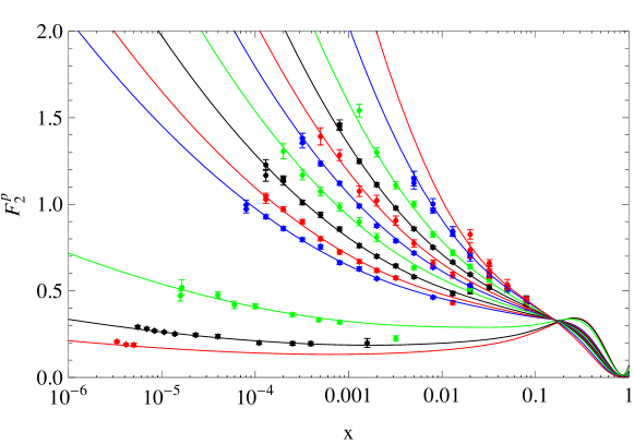
Adding the CTEQ6L valence contribution $F_{2v}$ to the $F_{2,{\rm asymp}}^{\gamma p}$ from the fit, we then obtain $F_{2}^{\gamma p}(x,Q^{2})$. Plots of the resulting $F_{2}^{\gamma p}(x,Q^{2})$ versus $x$ are shown in Fig. 1 along with the all the corresponding (unsifted) HERA data for representative values of $Q^{2}$, $Q^{2}$=0.15, 0.25, 0.65, 3.5, 4.5, 6.5, 10, 15, 22, 35, 70, 250, and 1200 GeV².

Although not shown in the figure, we find that this fit and our published fit Block et al. (2010, 2011) using the expression in Eq. (5)—not valid for small $Q^{2}$—agree in the region where there are HERA data. The present results behave properly at smaller $Q^{2}$ and in the valence-dominated region $x\gtrsim 0.1$, which the earlier results did not. We also note the appearance of at quasi fixed point in the fit at $x\approx 0.11$ where the rise in the valence distribution with increasing $x$ approximately compensates for the sharp fall in the asymptotic distribution. This appeared automatically; it was imposed in Eq. (5).

The validity of this fit to $F_{2}^{\gamma p}$ could be checked in the future at the proposed Large Hadron-electron Collider (LHeC) Abolleir Fernandez et al. (2012) over ranges of $x$ and $Q^{2}$ larger by roughly a factor of 20 than those accessible at HERA.

Figure 1: Plots of the fitted proton structure function, $F_{2}^{\gamma p}(x,Q^{2})$ versus Bjorken $x$ for virtualities, bottom to top, $Q^{2}$=0.15, 0.25, 0.65, 3.5, 4.5, 6.5, 10, 15, 22, 35, 70, 250, and 1200 GeV².

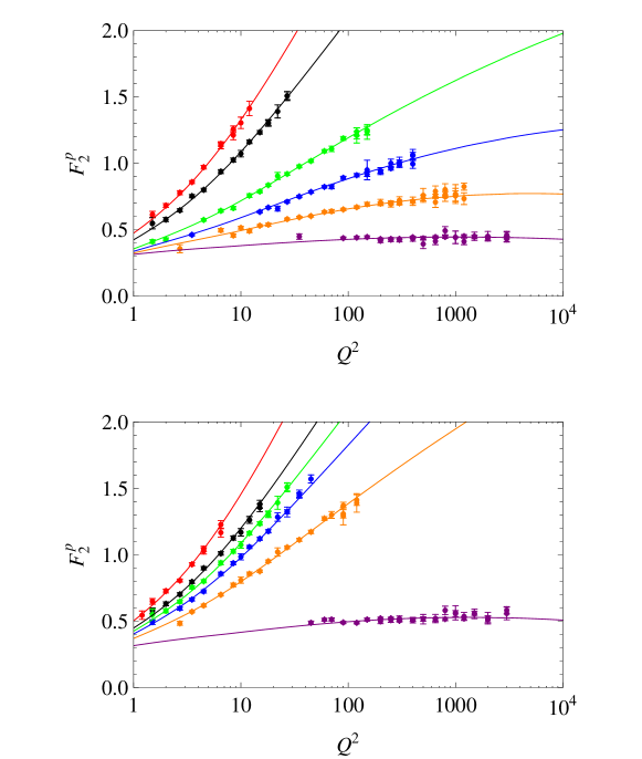
Plots of the fitted $F_{2}^{\gamma p}(W,Q^{2})$ are shown as functions of $Q^{2}$ and $W$, along with the HERA data, for representative values of $x$ and $Q^{2}$ in Figs. 2 and 3. The fits are clearly very good as is reflected by the excellent overall $\chi^{2}$ and fit probability. The curves in Fig. 2 also extend smoothly and reasonably to values of $Q^{2}\gtrsim 10^{4}$ GeV² above those measured, but needed in our later calculations of neutrino cross sections.

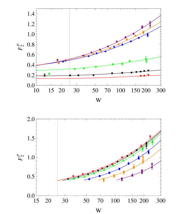
In the less conventional plots of $F_{2}^{\gamma p}$ in Fig. 3, the effects of the restrictions $W\geq 25$ GeV and $x\leq 0.1$ are clear. All the data at the given values of $Q^{2}$ are shown, with the $W$ cutoff indicated in each figure by the vertical line, and the solid curves in Fig. 3 stopping at the lowest $W$ for which $x<0.1$. It is again obvious that the model describes the HERA combined data very well, even, in the upper panel, for $W<25$ GeV. We note finally that the results are changed very little by increasing the $W$ cutoff to $W=30$ or 35 GeV.

Figure 2: Plots of our fit to $F_{2}^{\gamma p}$ as a function of $Q^{2}$ at fixed $x$, compared to the corresponding HERA data Aaron et al. (2010). Top panel, top to bottom: $x=0.0002$ (red), 0.0005 (black), 0.0032 (green), 0.008 (blue), 0.02 (orange), 0.08 (purple); Bottom panel, top to bottom: $x=0.00013$ (red), 0.00032 (black), 0.0005 (green), 0.0008 (blue), 0.002 (orange), 0.05 (purple).

Figure 3: Plots of the fitted proton structure function $F_{2}^{\gamma p}(W,Q^{2})$ versus $W$ for representative values of $Q^{2}$. The vertical lines indicate the cutoff used in the fit, $W\geq 25$ GeV. In the upper panel, top to bottom: $Q^{2}=0.15$ (red), $0.25$ (black), $0.65$ (green), $3.5$ (blue), $4.5$ (orange), and $6.5$ (purple) GeV² In the lower panel: top to bottom: $Q^{2}=35$ (red), $90$ (black), $120$ (green), $250$ (blue), $500$ (orange), and $1200$ (purple) GeV². The curves in this panel extend in $W$ only to the minimum value allowed by the condition $x\leq 0.1$. All data at the specified values of $Q^{2}$ are shown.

IV Applications

IV.1 $\gamma^{*}p$ cross sections from the fit

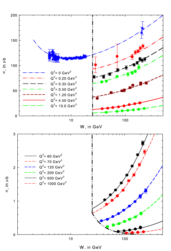
It is straightforward to evaluate the $\gamma^{*}p$ cross section, Eq. (4), using $F_{2}^{\gamma p}(W,Q^{2})$ from the fit. In Fig. 4, we show plots of the $\gamma^{*}p$ cross sections vs. $W$, the center of mass energy of the $\gamma^{*}p$ system, for representative values of $Q^{2}$ up to 10 GeV² in the upper curves, and $Q^{2}=60$ to 1000 GeV² in the lower curves. The upper curve for $Q^{2}=0$ is the Block-Halzen fit 2 Block and Halzen (2004) to the real $\gamma p$ cross section, shown with the all of the data for $W\geq 2$ GeV. Because of the constraints we have imposed on our fit parameters in Eq. (15), using the Block-Halzen parameters as input, our results agree exactly with the asymptotic part of the of the Block-Halzen fit at $Q^{2}=0$. The added Regge-like term is only 3.5% of the cross section at $W=25$ GeV, and decreases as $1/W$ for larger $W$, so is essentially negligible on the scale of the figure.

Figure 4: Plots of the $\gamma^{*}p$ cross section $\sigma^{\gamma^{*}p}$, in $\mu$b. vs. $W$, the cms energy of the $\gamma^{*}p$ system. The upper curve is for $Q^{2}$ = 0 to 10 GeV²; the lower curve is for $Q^{2}=60$ to 1000 GeV². Notice the very different scales of the vertical axes (cross sections) of the two curves. The circles which are plotted for Q${}^{2}\neq 0$ are $\gamma^{*}p$ cross section data from HERA DIS (deep inelastic scattering) that satisfy the cuts $W\geq 25$ GeV and $x\leq 0.1$; the $W$ cut for the curves is indicated by the thick dot-dot-dashed vertical line in the upper plot and the thick dot-dot-dashed boundary in the lower plot . The plotted cross section curves of $\sigma^{\gamma^{*}p}$ for $Q^{2}>0$ are the sum of the asymptotic cross section plus the valence cross section. For $Q^{2}=0$, the curve is the sum of the asymptotic DIS cross section plus the rapidly decreasing Regge-like term used in the Block-Halzen fit to real $\gamma p$ data Block and Halzen (2004); the data for $W>2$ GeV are shown as (blue) triangles.

.

It is evident from this figure, plotted on a logarithmic scale in $W$, that the data follow the quadratic curves in $\ln{W}$ given by our asymptotic form for $F_{2}^{\gamma p}$, Eq. (8), with the shapes changing smoothly as a function of $Q^{2}$ and approaching the $\gamma p$ cross section for $Q^{2}\rightarrow 0$. This indicates that the Froissart type behavior characteristic of high-energy hadronic interactions and $\gamma p$ scattering persists experimentally into the region of virtual $\gamma^{*}p$ scattering, as argued in Berger et al. (2007); Block et al. (2010, 2011) and discussed in more detail in Block et al. (2013a). A direct calculation of the $\gamma p$ cross section using a parton-level description Honjo et al. (1993) to account for the rise in the cross section with increasing $W$ in fact demonstrates the onset of the Froissart type behavior theoretically in that case.

IV.2 $e^{\pm}p$ neutral current cross sections

The integrated $e^{\pm}p$ neutral current (NC) cross sections are of potential interest for $ep$ collider experiments. These involve integrals over the doubly differential cross section Klein and Riemann (1984); Abramowicz et al. (2013)

$$\frac{d^{2}\sigma^{e^{\pm}p}_{NC}}{dxdQ^{2}}(E_{e},Q^{2},x)=\frac{2\pi\alpha^{2}}{Q^{4}}\frac{1}{x}[Y_{+}\tilde{F_{2}}(x,Q^{2})\mp Y_{-}x\tilde{F_{3}}(x,Q^{2})-y^{2}\tilde{F_{L}}(x,Q^{2})],$$ (16)

where $\alpha$ is the fine-structure constant, $Y_{\pm}=1\pm(1-y)^{2}$, $y=Q^{2}/2mE_{e}=Q^{2}/2e\cdot p$, and $\tilde{F_{2}}(x,Q^{2})$, $\tilde{F_{3}}(x,Q^{2})$ and $\tilde{F_{L}}(x,Q^{2})$ are generalized structure functions which include $Z$ as well as $\gamma$ exchanges between the incident electron and the proton. Next-to-leading (NLO) order QCD calculations predict that the contribution of the longitudinal structure function, $\tilde{F_{L}}$, to $d^{2}\sigma/dxdQ^{2}$ is $<1\%$ Klein and Riemann (1984).

The generalized structure functions can be split into terms depending on $\gamma$ exchange ($F_{2}^{\gamma}$), $Z$ exchange ($F_{2}^{Z}$, $xF_{3}^{Z}$) and $\gamma/Z$ interference ($F_{2}^{\gamma Z}$, $xF_{3}^{\gamma Z}$) as

$$\tilde{F_{2}}=F_{2}^{\gamma}-v_{e}P_{Z}F_{2}^{\gamma Z}+(v_{e}^{2}+a_{e}^{2}){P_{Z}^{2}}F_{2}^{Z},$$ (17)

$$x\tilde{F_{3}}=-a_{e}P_{Z}xF_{3}^{\gamma Z}+2v_{e}a_{e}{P_{Z}^{2}}xF_{3}^{Z}.$$ (18)

The standard model predictions for vector and axial vector couplings of the electron to the $Z$ boson are $v_{e}=-1/2+2\sin^{2}\theta_{W}$ and $a_{e}=-1/2$, where $\theta_{W}$ is the Weinberg angle; we use $\sin^{2}\theta_{W}=0.231$. The relative fraction of events coming from $Z$ exchange relative to $\gamma$ exchange is given at fixed $Q^{2}$ by Abramowicz et al. (2013)

$$P_{Z}=\frac{1}{\sin^{2}{2\theta_{W}}}\frac{Q^{2}}{M_{Z}^{2}+Q^{2}}.$$ (19)

The structure functions can be written at the bare quark level, before QCD corrections, in terms of the sum and differences of the quark and anti-quark momentum distributions,

$$[F_{2}^{\gamma},F_{2}^{\gamma Z},F_{2}^{Z}]=\sum_{q}[e_{q}^{2},2e_{q}v_{q},v_{q}^{2}+a_{q}^{2}]x(q+\bar{q}),$$ (20)

$$[xF_{3}^{\gamma Z},xF_{3}^{Z}]=\sum_{q}[e_{q}a_{q},v_{q}a_{q}]2x(q-\bar{q}),$$ (21)

where the sum runs over all quark flavors except the top quark which is too massive to contribute significantly in the region of interest; $e_{q}$ is the electric charge of the quark and $v_{q}$ and $a_{q}$ are the respective vector and axial couplings of the quark $q$ to the $Z$ boson. For $q=u$, $c$, and $t$, the Standard Model values of the respective vector and axial couplings are $v_{q}=1/2-4/3\sin^{2}\theta_{W}$ and $a_{q}=1/2$. For $q=d$, $s$, and $b$, we have $v_{q}=-1/2+2/3\sin^{2}\theta_{W}$ and $a_{q}=-1/2$.

Following the procedures discussed in Block et al. (2013a), we can re-express the structure functions given at the quark level in Eq. (20) and Eq. (21), in terms of $F_{2}^{\gamma p}$, a valence term $U$, and a set of non-singlet quark distributions $T_{8}$, $T_{15}$, and $T_{24}$ which can be determined from $F_{2}^{\gamma p}$ with minimal input. We have $F_{2}^{\gamma}=F_{2}^{\gamma p}$ in Eqs. (17) and (18),

$$F_{2}^{\gamma Z} = (3-\frac{20}{3}\sin^{2}{\theta_{W}})F_{2}^{\gamma p}-\frac{4}{27}\sin^{2}{\theta_{W}}T_{8}-\frac{2}{9}\sin^{2}{\theta_{W}}U,\qquad n_{f}=3,$$

$$F_{2}^{\gamma Z} = (3-\frac{36}{5}\sin^{2}{\theta_{W}})F_{2}^{\gamma p}+\frac{16}{135}\sin^{2}{\theta_{W}}\left(T_{15}-T_{8}\right)-\frac{2}{9}\sin^{2}{\theta_{W}}U,\qquad n_{f}=4,$$ (22)

$$F_{2}^{\gamma Z} = (3-\frac{76}{11}\sin^{2}{\theta_{W}})F_{2}^{\gamma p}-\frac{8}{297}\sin^{2}{\theta_{W}}\left(5T_{8}-5T_{15}+3T_{24}\right)-\frac{2}{9}\sin^{2}{\theta_{W}}U,\qquad n_{f}=5,$$

with $F_{2}^{\gamma p}$ the measured (fitted) DIS structure function, and

$$F_{2}^{Z} = (\frac{9}{4}-4\sin^{2}{\theta_{W}}+4\sin^{4}{\theta_{W}})F_{2}^{\gamma p}-(9-8\sin^{2}{\theta_{W}})(\frac{1}{72}T_{8}+\frac{1}{48}U),\qquad n_{f}=3,$$

$$F_{2}^{Z} = (\frac{9}{5}-\frac{18}{5}\sin^{2}{\theta_{W}}+4\sin^{4}{\theta_{W}})F_{2}^{\gamma p}+(9-8\sin^{2}{\theta_{W}})(\frac{1}{90}\left(T_{15}-T_{8}\right)-\frac{1}{48}U),\qquad n_{f}=4,$$ (23)

$$F_{2}^{Z} = (\frac{45}{22}-\frac{41}{11}\sin^{2}{\theta_{W}}+4\sin^{4}{\theta_{W}})F_{2}^{\gamma p}-(9-8\sin^{2}{\theta_{W}})(\frac{1}{396}\left(5T_{8}-5T_{15}+3T_{24}\right)-\frac{1}{48}U),\qquad n_{f}=5.$$

The $xF_{3}$ terms involve only the valence distribution $U$ with

$$F_{3}^{\gamma Z}=\frac{3}{2}U\,\,,\,\,F_{3}^{Z}=(\frac{3}{4}-\frac{5}{3}\sin^{2}{\theta_{W}})U;$$ (24)

their contributions to the total $e^{\pm}p$ neutral current cross sections are negligible. The structure function $\tilde{F_{L}}$, which is zero in LO, is given in NLO by

$$x^{-1}\tilde{F_{L}}(x,Q^{2})=\frac{\alpha_{s}}{2\pi}C_{Lq}\otimes(x^{-1}F_{20}^{\gamma})+\frac{\alpha_{s}}{2\pi}2n_{f}\,C_{Lg}\otimes g.\\$$ (25)

The details are discussed in Block et al. (2013b).

The $\gamma/Z$ interference term and the pure $Z$ exchange term will give small contributions to the complete $e^{\pm}p$ cross section, so it is sufficient to estimate them using the “wee-parton” approximation in which the quark distributions are taken as equal at small $x$. This is equivalent to setting the $T_{i}$ and $U$ terms in Eqs. (IV.2)–(23) equal to zero Block et al. (2013b). The $\gamma Z$ interference term and the $Z$ exchange term are then expressed simply in terms of numerical multiples of $F_{2}^{\gamma p}$, which is known. The longitudinal structure function $\tilde{F_{L}}$ can be treated similarly.

With this input, it is straightforward to evaluate the NC $e^{\pm}p$ cross section by integrating the expression in Eq. (16) over $x$ and $Q^{2}$. The $\gamma$ exchange contribution diverges as $1/Q^{2}$ for $Q^{2}\rightarrow 0$; we use a lower bound on the $Q^{2}$ integration $Q_{0}^{2}=1$ GeV². In Table 2, we show the resulting values of the NC $e^{\pm}p$ cross section over the energy range from $E_{e}=10^{6}$ GeV up to $E_{e}=10^{12}$ GeV, corresponding to center-of-mass energies in the $ep$ system from 1.4 TeV to 1400 TeV. Contributions from $F_{2}^{\gamma}$ , $Z$ exchange $F_{2}^{Z}$, $\gamma/Z$ interference $F_{2}^{\gamma Z}$, and $\tilde{F_{L}}$, to the total $e^{\pm}p$ cross section are also given in the Table. Contributions from the $F_{3}$ terms and the valence term $U$ are very small so can be ignored. As expected, dominant contributions are from the $F_{2}^{\gamma}$ term.

Table 2: Neutral current $e^{\pm}p$ cross section for $Q^{2}>1$ GeV², in cm², as a function of $E_{e}$, the laboratory energy, in GeV. $\sigma^{e^{\pm}p}$ is the total neutral current cross sections. $\sigma_{F_{2}}$, $\sigma_{F_{L}}$, $\sigma_{F_{2}^{\gamma Z}}$, and $\sigma_{F_{2}^{Z}}$ are the contributions from $F_{2}^{\gamma}$, $\tilde{F_{L}}$, $F_{2}^{\gamma Z}$, and $F_{2}^{Z}$ respectivly.

$E_{e}$ (GeV)	$\sigma^{e^{\pm}p}({\rm cm^{2}})$	$\sigma_{F_{2}}({\rm cm^{2}})$	$\sigma_{F_{L}}({\rm cm^{2}})$	$\sigma_{F_{2}^{\gamma Z}}({\rm cm^{2}})$	$\sigma_{F_{2}^{Z}}({\rm cm^{2}})$
$10^{6}$	$2.59\times 10^{-30}$	$2.12\times 10^{-30}$	$1.82\times 10^{-32}$	$5.90\times 10^{-32}$	$3.88\times 10^{-31}$
$10^{7}$	$3.91\times 10^{-30}$	$3.22\times 10^{-30}$	$2.17\times 10^{-32}$	$8.80\times 10^{-32}$	$5.84\times 10^{-31}$
$10^{8}$	$5.70\times 10^{-30}$	$4.73\times 10^{-30}$	$2.51\times 10^{-32}$	$1.23\times 10^{-31}$	$8.21\times 10^{-31}$
$10^{9}$	$8.02\times 10^{-30}$	$6.73\times 10^{-30}$	$2.83\times 10^{-32}$	$1.64\times 10^{-31}$	$1.10\times 10^{-30}$
$10^{10}$	$1.10\times 10^{-29}$	$0.93\times 10^{-29}$	$3.13\times 10^{-32}$	$2.11\times 10^{-31}$	$1.42\times 10^{-30}$
$10^{11}$	$1.46\times 10^{-29}$	$1.25\times 10^{-29}$	$3.43\times 10^{-32}$	$2.64\times 10^{-31}$	$1.78\times 10^{-30}$
$10^{12}$	$1.91\times 10^{-29}$	$1.65\times 10^{-29}$	$3.72\times 10^{-32}$	$3.23\times 10^{-31}$	$2.18\times 10^{-30}$

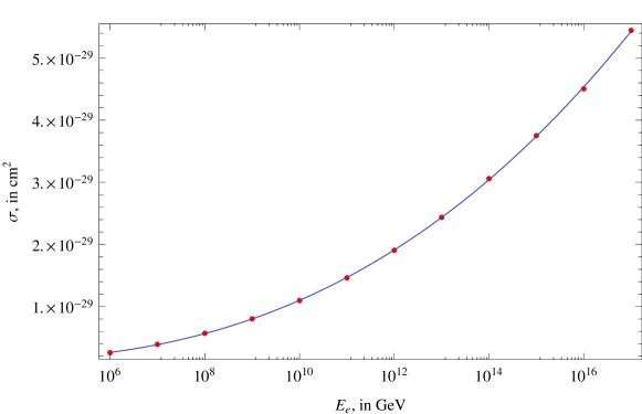
The integration of the doubly differential cross section in Eq. (16) over $x$ and $Q^{2}$ needed to obtain these results involves a factor $dx/x=d(\ln{x})$ from the pre factor $1/x$ in Eq. (16), with an upper limit on $x$ of $2mE_{e}/Q_{\rm min}^{2}$. The $Q^{2}$ integration converges rapidly. As a result, a Froissart bounded $F_{2}^{\gamma p}$ which behaves asymptotically as $\ln^{2}(1/x)$ for decreasing $x$ leads to an integrated $ep$ cross section that grows asymptotically as $\ln^{3}E_{e}$. This modified Froissart behavior for the integrated cross sections was originally noted in the case of neutrino-proton scattering in Illarianov et al. (2011), where the bound on the integrated cross section is proportional to $\ln^{3}E_{\nu}$, and was re-emphasized for that case in Block et al. (2013b). More generally, the integrated $e^{\pm}p$ and $\nu N$ cross sections should behave asymptotically as $\ln^{3}E_{e}$ or $\ln^{3}E_{\nu}$, with sub-dominant terms which behave as lower powers of $\ln{E_{e}}$ or $\ln{E_{\nu}}$. We have therefore done a 4 parameter fit to the $e^{\pm}p$ cross section of the form $\sigma^{e^{\pm}p}=a+b\ln E_{e}+c\ln E_{e}^{2}+d\ln E_{e}^{3}$, using the data in Table 2 and its extension to higher $E_{e}$, to obtain the analytic expression for the integrated cross section for $Q^{2}>1$ GeV²,

$$\sigma^{e^{\pm}p}_{NC}(E_{e})=3.058\times 10^{-30}-3.593\times 10^{-31}\ln E_{e}+1.339\times 10^{-32}\ln^{2}E_{e}+7.472\times 10^{-34}\ln^{3}E_{e}.$$ (26)

Here $E_{e}$ is in GeV and the constants and cross section in cm². We plot the data from Table 2 and the fitted cross section in Fig. 5. The $\ln^{3}E_{e}$ parameterization is excellent, with numerical agreement better than 1 part in 1000. Detection of this behavior in $e^{\pm}p$ scattering would be a clear indication of a Froissart boundedness of the underlying $\gamma^{*}p$ cross section.

Figure 5: Plots of $e^{\pm}p$ NC cross section for $Q^{2}>1$ GeV², in cm², vs. $E_{e}$, the laboratory neutrino energy, in GeV. The points are the numerical calculations of Table 2.

IV.3 Neutrino-nucleon cross sections

The charged current (CC) and neutral current (NC) cross sections for the scattering of neutrinos and antineutrinos on an isoscalar nucleon target $N=(p+n)/2$ at ultra-high energies have been calculated by a number of authors using different approaches. The results depend on the behavior of structure functions at ultra-small $x$, down to $x\sim 10^{-12}$ for the neutrino energies $E_{\nu}\sim 10^{16}$ GeV that will potentially be accessible at cosmic ray neutrino detectors now operating (ICECUBE Achterberg et al. (2007), Baikal Spearing et al. (2005), ANTARES Aguilar et al. (2007), HiRes Abbasi et al. (2008), AUGER Pastor et al. (2012)), or under development (ARA Allison et al. (2012), ARIANNA Gerhart et al. (2010)) or proposed (JEM-EUSO Takahashi et al. (2009); Adams and other (2012)).

The cross section calculations of Reno and Quigg (1988); Frichter et al. (1995); Gandhi et al. (1996, 1998); Cooper-Sarkar and Sarkar (2008); Gluck et al. (2010); Cooper-Sarkar et al. (2011), which use parton distributions derived in analyses of DIS based on the DGLAP evolution equations Gribov and Lipatov (1972); Altarelli and Parisi (1977); Dokshitzer (1977), require the extrapolation of those power-law dominated parton distributions far outside the experimental region, with results that become increasingly uncertain at very high neutrino energies. Alternative approaches such as that of Fiore et al. Fiore et al. (2005, 2006) emphasize specific ideas about the behavior of structure functions at small $x$ which go beyond the usual DGLAP approach, and allow for parton recombination effects and the damping of structure functions at very small $x$ Gribov et al. (1983); des .

In the approach adopted here, we emphasize instead the expression of the neutrino cross sections directly in terms of a Froissart-bounded $F_{2}^{\gamma p}$ following Block et al. (2008P, 2010), with the inclusion of small corrections not considered there. We do not introduce a specific mechanism for the boundedness within the general Froissart framework. The calculations are discussed in detail in Block et al. (2013a) and Block et al. (2013b). We will not repeat the details or the arguments for this approach here, but simply present the results of updated calculations in which the fit to the HERA data on $F_{2}^{\gamma p}$ given in Block et al. (2010, 2011) is replaced by the fit constructed here.

IV.3.1 Numerical evaluation of the CC and NC $\nu N$ cross sections

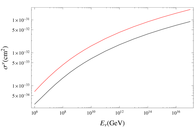
In Fig. 6 we show the $\nu N$ CC and NC cross sections, in cm², as a function of $E_{\nu}$, in GeV, for large $E_{\nu}$, calculated using our fit to $F_{2}^{\gamma p}$.

Figure 6: Plots of the $\nu N$ cross sections, in cm², versus $E_{\nu}$, the laboratory neutrino energy, in GeV, calculated using the extrapolation of the global fit to the HERA data on $F_{2}^{\gamma p}(x,Q^{2})$ to small $x$, and the relations between $F_{2}^{\nu(\bar{\nu})}$, $F0_{2}^{\nu(\bar{\nu})}$, and $F_{2}^{\gamma p}$ with NLO treatments of the small functions $T^{\prime}_{i}$ and of the subdominant structure functions $F_{3}^{\nu(\bar{\nu})}$ and $F_{L}^{\nu(\bar{\nu})}$ discussed in Block et al. (2013b). The upper curve (red) is the CC cross section and lower curve (black) is the NC cross section.

Table 3: Charged current $\nu N$ cross sections, in cm², as a function of $E_{\nu}$, the laboratory neutrino energy, in GeV. Here $\sigma_{CC}$ is the total charged current cross section. $\sigma_{F_{2}}$ , $\sigma_{F_{3}}$, $\sigma_{F_{L}}$, and $\sigma_{U}$ are the contributions from $F_{2}^{\nu}$, $F_{3}^{\nu}$, $F_{L}^{\nu}$ , and from the valence quark distribution $U$.

$E_{\nu}$ (GeV)	$\sigma_{CC}({\rm cm^{2}})$	$\sigma_{F_{2}}({\rm cm^{2}})$	$\sigma_{F_{3}}({\rm cm^{2}})$	$\sigma_{F_{L}}({\rm cm^{2}})$	$\sigma_{U}({\rm cm^{2}})$
$10^{6}$	$6.66\times 10^{-34}$	$6.97\times 10^{-34}$	$0.01\times 10^{-34}$	$-0.15\times 10^{-34}$	$-0.16\times 10^{-34}$
$10^{7}$	$1.83\times 10^{-33}$	$1.89\times 10^{-33}$	$0.00$	$-0.03\times 10^{-33}$	$-0.03\times 10^{-33}$
$10^{8}$	$4.31\times 10^{-33}$	$4.42\times 10^{-33}$	$0.00$	$-0.07\times 10^{-33}$	$-0.04\times 10^{-33}$
$10^{9}$	$8.87\times 10^{-33}$	$9.00\times 10^{-33}$	$0.00$	$-0.14\times 10^{-33}$	$0.00$
$10^{10}$	$1.61\times 10^{-32}$	$1.64\times 10^{-32}$	$0.00$	$-0.02\times 10^{-32}$	$0.00$
$10^{11}$	$2.69\times 10^{-32}$	$2.73\times 10^{-32}$	$0.00$	$-0.04\times 10^{-32}$	$0.00$
$10^{12}$	$4.19\times 10^{-32}$	$4.24\times 10^{-32}$	$0.00$	$-0.05\times 10^{-32}$	$0.00$
$10^{13}$	$6.19\times 10^{-32}$	$6.26\times 10^{-32}$	$0.00$	$-0.07\times 10^{-32}$	$0.00$
$10^{14}$	$8.77\times 10^{-32}$	$8.85\times 10^{-32}$	$0.00$	$-0.09\times 10^{-32}$	$0.00$
$10^{15}$	$12.0\times 10^{-32}$	$12.1\times 10^{-32}$	$0.00$	$-0.11\times 10^{-32}$	$0.00$
$10^{16}$	$15.9\times 10^{-32}$	$16.1\times 10^{-32}$	$0.00$	$-0.13\times 10^{-32}$	$0.00$
$10^{17}$	$20.7\times 10^{-32}$	$20.8\times 10^{-32}$	$0.00$	$-0.16\times 10^{-32}$	$0.00$

Table 4: Neutral current $\nu N$ cross sections, in cm², as a function of $E_{\nu}$, the laboratory neutrino energy, in GeV: $\sigma_{NC}$ is the total neutral current cross section. $\sigma_{F_{2}}$ , $\sigma_{F_{3}}$, $\sigma_{F_{L}}$, and $\sigma_{U}$ are the contributions from $F_{2}^{\nu}$, $F_{3}^{\nu}$, $F_{L}^{\nu}$ , and from the valence quark distribution $U$.

$E_{\nu}$ (GeV)	$\sigma_{NC}({\rm cm^{2}})$	$\sigma_{F_{2}}({\rm cm^{2}})$	$\sigma_{F_{3}}({\rm cm^{2}})$	$\sigma_{F_{L}}({\rm cm^{2}})$	$\sigma_{U}({\rm cm^{2}})$
$10^{6}$	$2.73\times 10^{-34}$	$2.75\times 10^{-34}$	$0.00$	$0.05\times 10^{-34}$	$-0.07\times 10^{-34}$
$10^{7}$	$7.14\times 10^{-34}$	$7.59\times 10^{-34}$	$0.00$	$-0.31\times 10^{-34}$	$-0.13\times 10^{-34}$
$10^{8}$	$1.71\times 10^{-33}$	$1.81\times 10^{-33}$	$0.00$	$-0.08\times 10^{-33}$	$-0.02\times 10^{-33}$
$10^{9}$	$3.59\times 10^{-33}$	$3.74\times 10^{-33}$	$0.00$	$-0.16\times 10^{-33}$	$0.00$
$10^{10}$	$6.63\times 10^{-33}$	$6.90\times 10^{-33}$	$0.00$	$-0.26\times 10^{-33}$	$0.00$
$10^{11}$	$1.12\times 10^{-32}$	$1.16\times 10^{-32}$	$0.00$	$-0.04\times 10^{-32}$	$0.00$
$10^{12}$	$1.76\times 10^{-32}$	$1.82\times 10^{-32}$	$0.00$	$-0.06\times 10^{-32}$	$0.00$
$10^{13}$	$2.62\times 10^{-32}$	$2.70\times 10^{-32}$	$0.00$	$-0.08\times 10^{-32}$	$0.00$
$10^{14}$	$3.73\times 10^{-32}$	$3.83\times 10^{-32}$	$0.00$	$-0.10\times 10^{-32}$	$0.00$
$10^{15}$	$5.12\times 10^{-32}$	$5.26\times 10^{-32}$	$0.00$	$-0.13\times 10^{-32}$	$0.00$
$10^{16}$	$6.84\times 10^{-32}$	$7.00\times 10^{-32}$	$0.00$	$-0.16\times 10^{-32}$	$0.00$
$10^{17}$	$8.91\times 10^{-32}$	$9.10\times 10^{-32}$	$0.00$	$-0.19\times 10^{-32}$	$0.00$

The values of the CC and NC cross sections over the energy range from $10^{6}$ GeV up to $10^{17}$ GeV are shown in Table 3 and Table 4 where contributions from $F_{2}^{\nu}$ , $F_{3}^{\nu(\bar{\nu})}$, $F_{L}^{\nu(\bar{\nu})}$, and the valence quark distribution $U$, to the total cross sections are also shown. Note that the contribution from $F_{3}^{\nu(\bar{\nu})}$ to the charged current neutrino cross section is very small and decreases as $E_{\nu}$ increases.

IV.3.2 Implications of high energy weak $\nu N$ scattering for strong hadronic interactions

Measurement of these new high energy neutrino cross section have the potential of allowing measurements of hadronic interactions and tests of the underlying theory at heretofore undreamt of high energies. In Fig. 7, we plot $W_{\rm rms}$, the CC root mean square cms energy of the strong interaction of the virtual vector boson, in TeV, against the energy $E_{\nu}$ of the laboratory neutrino, in GeV. We see in Fig 7 that for $E_{\nu}\approx 10^{10}$ GeV that we have already reached the strong interaction energy of $57$ TeV, the cms energy in $pp$ collisions reached by the Pierre Auger Collaboration Abreu et al. (2012) using cosmic ray protons with $E_{p}\sim 1.7\times 10^{18}$ eV, near the expected Greisen-Zatsepi-Kuzmin limit on the incident proton spectrum Greisen (1966); Zatsepin and Kuzmin (1966). The incident neutrino spectrum is not subject to this limit, and may well extend to much higher energies. Thus, for $E_{\nu}\approx 10^{10},\,10^{11},\,10^{12},\,10^{13},\,10^{14}$ GeV ($10^{19},\,10^{20},\,10^{21},\,10^{22},\,10^{23}$ eV), we are at a strong interaction cms energies $W_{\rm rms}\approx 54,\,160,\,480,\,1430$ and 4300 TeV, showing that the detection of ultra-high energy neutrinos would allow us to reach exceedingly high hadronic energies.

Figure 7: Plot of $W_{{\rm rms}}$, the root mean square hadronic cms energy of the virtual vector boson $-N$ system, in TeV, versus $E_{\nu}$, the laboratory neutrino energy for CC scattering, in GeV.

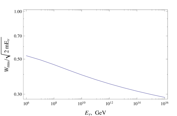
The conversion of the weak $\nu N$ cms energy into the cms energy of the virtual boson$\,N$ system is very efficient. In Fig. 8, we plot the fraction of the $\nu N$ cms energy that is in the final hadronic system, defined here as the ratio

$${\rm frac} = \left(\frac{\left<s\right>}{2mE_{\nu}}\right)^{1/2}=\frac{W_{\rm rms}}{\left(2mE_{\nu}\right)^{1/2}},$$ (27)

versus the laboratory neutrino energy $E_{\nu}$, in GeV. Here $W_{\rm rms}$ is the square root of $\left<s\right>$, the mean of the square of the cms hadronic energy of the virtual vector boson - isobaric nucleon $N$ system, and $2mE_{\nu}$ is the square of the cms energy of the $\nu N$ system. From Fig. 8, it is clear that a very large percentage, of the order of 50%, of the cms energy of the $\nu N$ system is found as hadronic energy for the lower energy neutrinos, decreasing to about 30 % at the highest energies.

Figure 8: Plot of the fraction $W_{{\rm rms}}/\sqrt{2mE_{\nu}}$ of the cms energy of the $\nu N$ system which appears in the hadronic cms energy of the virtual vector boson-$N$ system, versus $E_{\nu}$, the laboratory neutrino energy in CC scattering, in GeV.

Just as in the $ep$ system, a test for the Froissart bounded behavior of the structure function $F_{2}^{\gamma p}$ is in a $\ln^{3}E_{\nu}$ asymptotic growth of the $\nu N$ total cross sections. The present calculations give

$$\sigma_{CC} = -2.097\times 10^{-32}+4.703\times 10^{-33}\ln{E_{\nu}}-3.666\times 10^{-34}\ln^{2}{E_{\nu}}+1.010\times 10^{-35}\ln^{3}{E_{\nu}},$$ (28)

$$\sigma_{NC} = \ \ \,1.021\times 10^{-32}+2.239\times 10^{-33}\ln{E_{\nu}}-1.700\times 10^{-34}\ln^{2}{E_{\nu}}+4.534\times 10^{-36}\ln^{3}{E_{\nu}},$$ (29)

where the cross sections are in cm² and $E_{\nu}$ is in GeV. We estimate about a 1 to 4 % error in the above cross sections.

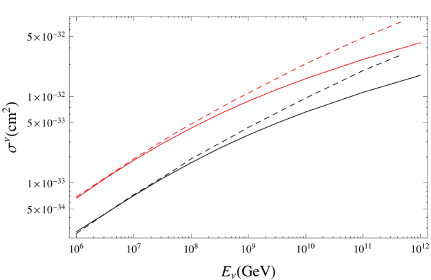
In Fig. 9 we compare our UHE (ultra-high-energy) cross sections from Fig. 6 with those of Cooper-Sarkar, Mertsch, and Sarkar (CSMS), who used the HERA-based PDF set HERAPDF1.5, and included the $b$ quark but not the $t$ in their computations. Their quoted error estimates are in the 2%-4% range, comparable to ours, when they exclude those PDF sets which lead to an unacceptably steep rise in the cross section or allow negative values of the gluon PDF at small $x$ and small $Q^{2}$. Note that our UHE cross sections are very close to the CSMS cross sections in the low energy region ($E_{\nu}<10^{7}$ GeV), eliminating a discrepancy encountered with our previous model for $F_{2}^{\gamma p}$ Block et al. (2013b).

Figure 9: Plots of $\nu N$ cross sections, in cm², vs. $E_{\nu}$, the laboratory neutrino energy, in GeV. Our CC cross section is the upper solid (red) curve and our NC cross section is the lower solid (black) curve; the CC cross section of CSMS is the upper dashed (red) curve and their NC cross section is the lower dashed (black) curve. All cross section calculations include the b-quark.

The strong divergence of the CSMS and present cross sections at UHE provides a clear distinction between cross sections based on standard parton distributions extrapolated to ultra-small $x$ and the cross sections based on the Froissart bound for strong hadronic processes presented here. They are an additional test of the strong interactions at exceedingly high energies.

V Summary and conclusions

Using a new Froissart-bounded parametrization of the DIS structure function $F_{2}^{\gamma p}$, we have fitted the the experimental HERA results on DIS Breitweg et al. (2000); Chekanov et al. (2001, 2003); Adloff et al. (2001) in the region $x\leq 0.1$ and $0.1\leq Q^{2}\leq 5000$ GeV², restricted to virtual $\gamma^{*}p$ center-of- mass energies $W\geq 25$ GeV. We have used the results to calculate the cross section $\sigma^{\gamma*p}(W,Q^{2})$ for virtual $\gamma^{*}p$ scattering, and connected it to the known Froissart-bounded high energy cross section for real $\gamma p$ scattering.

The new parametrization for $F_{2}^{\gamma p}$ is divided into two parts, an asymptotic (high energy) part corresponding to $W\geq 25$ GeV and $x\leq 0.1$ and a low energy part corresponding to the valence-quark contributions. Our parameterization of $F_{2}^{\gamma p}$ requires that $F_{2}^{\gamma p}\rightarrow 0$ as $Q^{2}\rightarrow 0$. In the fitting procedure, we also require that when $Q^{2}\rightarrow 0$, the asymptotic portion of $\sigma^{\gamma^{*}p}(W,Q^{2})\rightarrow 0$ go smoothly into the measured asymptotic real $\gamma p$ cross section $\sigma^{\gamma p}(W)$, found by Block-Halzen Block and Halzen (2004) to be of the form $c_{0}^{BH}+c_{1}^{BH}\ln(\nu/m)+c_{2}^{BH}\ln^{2}(\nu/m)$, where $\nu$ is the $\gamma$ laboratory energy. This fixes 3 of the 12 parameters used in the asymptotic part of $F_{2}^{\gamma p}$. The valence contributions are then added to obtain the full parametrization of $F_{2}^{\gamma p}$. A $\chi^{2}$ fit to the 395 HERA datum points with $W\geq 25$ GeV and $x<0.1$ (with 9 free parameters) gives a $\chi^{2}/{\rm d.o.f.}=0.95$, with a goodness-of-fit probability of 0.76.

The fit also determines the mass parameter $M$ of Eq. (12). This mass specifies the most important mass region in the dispersion relation for $F_{2}^{\gamma p}$ in $Q^{2}$, and can be interpreted as the effective mass of the virtual vector boson (or group of bosons) that interacts strongly with the nucleon. The result is $M=0.87$ GeV, in the mass region covered by the vector mesons $\rho,\ \omega$ and $\phi$, a result compatible with the idea of vector meson dominance.

Since the asymptotic portion of $\sigma^{\gamma^{*}p}(W,Q^{2})$ was constructed to be compatible with a Froissart bound of $\ln^{2}W$, so is the high energy portion of the fit to $F_{2}^{\gamma p}(x,Q^{2})$. In particular, for small $x$ and all $Q^{2}\geq 0$, $F_{2}^{\gamma p}(x,Q^{2})$ is bounded by $\ln^{2}(1/x)$.

We use our new results on $F_{2}^{\gamma p}$ to calculate the $ep$ cross section, and update earlier calculations Block et al. (2013b) of $\nu N$ cross sections. For high initial energies of either the $ep$ or $\nu N$ collisions, the integration over the Froissart-bounded structure function proportional to $\ln^{2}(1/x)$ needed to obtain the total cross section gives a high energy total cross section $\sigma(E)$ bounded by $\ln^{3}E$ where $E$ is the laboratory energy of the electron or neutrino, i.e., $\sigma(E)=\alpha+\beta\ln E+\gamma\ln^{2}E+\delta\ln^{3}E$, providing a new test for the boundedness. In a certain sense, this is a new type of unification of the electromagnetic and weak interactions, brought about by the high energy cross sections for both being controlled by the Froissart bound on hadronic processes. In essence, the strong interactions determine both the weak and electromagnetic cross sections up to factors of the electroweak gauge boson - nucleon couplings. It is possible that these considerations can be extended to quantum gravitational interactions through the exchange of a spin 2 graviton. The virtual graviton would effectively interact strongly—up to the gravitational coupling—with hadrons. A possible example would be the gravitational interaction of high energy sterile neutrinos with nucleons.

We emphasize that measuring ultra-high energy neutrino $-N$ cross sections would allow us to investigate strong interactions, i.e., the hadronic Froissart bound, at incredibly high energies, opening up new techniques for studying high energy hadron physics. For example, if one were able to measure the total cross section for neutrino interactions at $E_{\nu}=10^{14}$ GeV, it would allow a measurement of the Froissart bound at $\approx 4000$ TeV.

References

• Breitweg et al. (2000) J. Breitweg et al. (ZEUS Collaboration), Phys. Lett. B 487, 53 (2000).
• Chekanov et al. (2001) S. Chekanov et al. (ZEUS Collaboration), Eur. Phys. J. C 21, 443 (2001).
• Chekanov et al. (2003) S. Chekanov et al. (ZEUS Collaboration), Phys. Rev. D 70, 052001 (2003).
• Adloff et al. (2001) C. Adloff et al. (H1 Collaboration), Eur. Phys. J. C 21, 33 (2001).
• Block et al. (2006) M. M. Block, E. L. Berger, and C.-I. Tan, Phys. Rev. Lett. 97, 252003 (2006), eprint hep-ph/0610296.
• Berger et al. (2007) E. L. Berger, M. M. Block, and C.-I. Tan, Phys. Rev. Lett. 98, 242001 (2007), eprint hep-ph/0703003.
• Block et al. (2010) M. Block, P. Ha, and D. McKay, Phys. Rev. D 82, 077302 (2010).
• Block et al. (2011) M. M. Block, L. Durand, P. Ha, and D. W. McKay, Phys. Rev. D 84, 094010 (2011).
• Block et al. (2013a) M. M. Block, L. Durand, P. Ha, and D. W. McKay, Phys. Rev. D 88, 014006 (2013a), eprint arXiv:1302.6119v2 [hep-ph].
• Froissart (1961) M. Froissart, Phys. Rev. 123, 1053 (1961).
• Martin (1963) A. Martin, Phys. Rev. 129, 1432 (1963).
• Jin and Martin (1964) Y. S. Jin and A. Martin, Phys. Rev. 135, 1375 (1964).
• Martin (1966) A. Martin, Nuovo Cimento 42, 930 (1966).
• Block (2006a) M. M. Block, Phys. Rep. 436, 71 (2006a).
• Block (2011) M. Block, Phys. Rev. D 84, 091501 (2011).
• Block and Halzen (2011) M. M. Block and F. Halzen, Phys. Rev. Lett. 107, 212002 (2011).
• Block and Halzen (2004) M. M. Block and F. Halzen, Phys. Rev. D 70, 091901 (2004), eprint hep-ph/0405174.
• Block et al. (1999) M. M. Block, E. M. Gregores, F. Halzen, and G. Pancheri, Phys. Rev. D 60, 054024 (1999).
• Aaron et al. (2010) F. D. Aaron et al. (H1 and ZEUS), JHEP 1001, 109 (2010), eprint arXiv:0911.0884 [hep-ex].
• Ashok suri (1971) Ashok suri , Phys. Rev. D 4, 570 (1971).
• Damashek and Gilman (1970) M. Damashek and F. J. Gilman, Phys. Rev. D 1, 1319 (1970).
• Aid et al. (1997) S. Aid et al. (H1 Collaboration), Z. Phys.C 75, 421 (1997).
• Chekanov et al. (2002) S. Chekanov et al. (ZEUS Collaboration), Nucl. Phys. B 627, 3 (2002).
• Stump et al. (2003) D. Stump, J. Huston, J. Pumplin, W. Tung, H. Lai, S. Kuhlmann, and J. Owens, J. High Energy Phys. 0310, 046 (2003), eprint [hep-ph/0303013].
• (25) http://durpdg.dur.ac.uk/hepdata/mrs.html.
• Block (2006b) M. M. Block, Nucl. Inst. and Meth. A. 556, 308 (2006b).
• Abolleir Fernandez et al. (2012) J. L. Abolleir Fernandez et al., J. Phys. G 39, 075001 (2012).
• Honjo et al. (1993) K. Honjo, L. Durand, R. Gandhi, H. Pi, and I. Sarcevic, Phys. Rev. D 48, 1048 (1993).
• Klein and Riemann (1984) M. Klein and T. Riemann, Z. Phys. C 24, 151 (1984).
• Abramowicz et al. (2013) H. Abramowicz et al., Phys. Rev. D 87, 052014 (2013).
• Block et al. (2013b) M. M. Block, L. Durand, P. Ha, and D. W. McKay, Phys. Rev. D 88, 013003 (2013b), eprint arXiv:1302.6127v2 [hep-ph].
• Illarianov et al. (2011) A. Illarianov, B. Kniehl, and A. Kotikov, Phys. Rev. Lett. 106, 231802 (2011).
• Achterberg et al. (2007) A. Achterberg et al. (ICECUBE Collaboration), Phys. Rev. D 76, 027101 (2007).
• Spearing et al. (2005) C. Spearing et al. (Baikal Collaboration), Nucl. Phys. B Proc. Suppl. 138, 175 (2005).
• Aguilar et al. (2007) J. A. Aguilar et al. (ANTARES Collaboration), Nucl. Inst. Meth. Phys. Res., Sec. A 570, 107 (2007).
• Abbasi et al. (2008) R. Abbasi et al. (HiRes Collaboration), Ap. J. 684, 790 (2008).
• Pastor et al. (2012) S. Pastor et al. (Pierre Auger Collaboration), Nucl.Instrum. Meth. A662, S113 (2012).
• Allison et al. (2012) P. Allison et al. (ARA Collaboration), Astropart. Phys. 35, 457 (2012).
• Gerhart et al. (2010) L. Gerhart et al. (ARIANNA Collaboration), Nucl. Inst. Meth. A 624, 85 (2010).
• Takahashi et al. (2009) Y. Takahashi et al. (EUSO Collaboration), New J. Phys. 11, 065009 (2009).
• Adams and other (2012) J. Adams and other (2012), eprint arXiv:1203.3451v2 [astro-ph.IM].
• Reno and Quigg (1988) M. H. Reno and C. Quigg, Phys. Rev. D 37, 657 (1988).
• Frichter et al. (1995) G. Frichter, D. McKay, and J. Ralston, Phys. Rev. Lett. 74, 1508 (1995).
• Gandhi et al. (1996) R. Gandhi, C. Quigg, M. H. Reno, and I. Sarcevic, Astropart. Phys. 5, 81 (1996).
• Gandhi et al. (1998) R. Gandhi, C. Quigg, M. H. Reno, and I. Sarcevic, Phys. Rev. D 58, 093009 (1998).
• Cooper-Sarkar and Sarkar (2008) A. Cooper-Sarkar and S. Sarkar, JHEP p. 0801:075 (2008).
• Gluck et al. (2010) M. Gluck, P. Jimenez-Delgado, and E. Reya, Phys. Rev. D 81, 097501 (2010).
• Cooper-Sarkar et al. (2011) A. Cooper-Sarkar, P. Mertsch, and S. Sarkar, JHEP p. 1108:42 (2011).
• Gribov and Lipatov (1972) V. N. Gribov and L. N. Lipatov, Sov. J. Nucl. Phys. 15, 438 (1972).
• Altarelli and Parisi (1977) G. Altarelli and G. Parisi, Nucl. Phys. B 126, 298 (1977).
• Dokshitzer (1977) Y. L. Dokshitzer, Sov. Phys. JETP 46, 641 (1977).
• Fiore et al. (2005) R. Fiore, L. L. Jenkovszky, A. V. Kotikov, F. Paccanoni, A. Papa, and E. Predazzi, Phys. Rev. D 71, 033002 (2005).
• Fiore et al. (2006) R. Fiore, L. L. Jenkovszky, A. V. Kotikov, F. Paccanoni, and A. Papa, Phys. Rev. D 73, 053012 (2006).
• Gribov et al. (1983) L. Gribov, E. Levin, and M. Ryskin, Phys. Reports 100, 1 (1983).
• (55) For a broad range of topics on small-x𝑥x physics, see Small x behavior of deep inelastic structure functions in QCD in Proceedings of the DESY Topical Meeting, Hamburg, F.R. Germany, 1990, edited by A. Ali and J. Bartels (Nucl. Phys. B, Proc. Suppl. 18C).
• Block et al. (2008P) M. M. Block, E. L. Berger, D. W. McKay, and C.-I. Tan, Phys. Rev. D 77, 053007 (2008P), eprint arXiv: 0708.1960v1 [hep-ph].
• Abreu et al. (2012) P. Abreu et al. (Pierre Auger Collaboration), Phys. Rev. Lett. 109, 062002 (2012), eprint arXiv:1208.1520 [hep-ex].
• Greisen (1966) K. Greisen, Phys. Rev. Lett. 16, 748 (1966).
• Zatsepin and Kuzmin (1966) G. T. Zatsepin and V. A. Kuzmin, Sov. Phys. JETP Lett. 4, 78 (1966).
• (60) M. M. Block, P. Ha and D. W. McKay, arXiv:1110.6665 [hep-ph] (2011).