Analysis of Schwarz methods for a hybridizable discontinuous Galerkin discretization

Abstract

Schwarz methods are attractive parallel solvers for large scale linear systems obtained when partial differential equations are discretized. For hybridizable discontinuous Galerkin (HDG) methods, this is a relatively new field of research, because HDG methods impose continuity across elements using a Robin condition, while classical Schwarz solvers use Dirichlet transmission conditions. Robin conditions are used in optimized Schwarz methods to get faster convergence compared to classical Schwarz methods, and this even without overlap, when the Robin parameter is well chosen. We present in this paper a rigorous convergence analysis of Schwarz methods for the concrete case of hybridizable interior penalty (IPH) method. We show that the penalization parameter needed for convergence of IPH leads to slow convergence of the classical additive Schwarz method, and propose a modified solver which leads to much faster convergence. Our analysis is entirely at the discrete level, and thus holds for arbitrary interfaces between two subdomains. We then generalize the method to the case of many subdomains, including cross points, and obtain a new class of preconditioners for Krylov subspace methods which exhibit better convergence properties than the classical additive Schwarz preconditioner. We illustrate our results with numerical experiments.

1 Introduction

We consider the elliptic model problem

(1) $$\begin{array}[]{rcll}\eta(x)u(x)-\nabla\cdot(a(x)\nabla u)&=&f,&\textrm{in $\Omega\subset\mathbb{R}^{2}$},\\ u&=&0,&\textrm{on $\partial\Omega$},\end{array}$$

in the weak sense where $f\in\textrm{L}^{2}(\Omega)$, $a(x)\in L^{\infty}(\Omega)$ and uniformly positive, $\eta_{0}\geq\eta(x)\geq 0$ and $\Omega$ is assumed to be a convex polygon for simplicity. Any discretization of this problem, for example by a finite element method (FEM) or a discontinuous Galerkin (DG) method, leads to a large sparse linear system

(2) $$A{\boldsymbol{u}}={\boldsymbol{f}},$$

where ${\boldsymbol{u}}$ is the vector of degrees of freedom representing an approximation of $u$ and $A$ represents the disretized differential operator. In this paper we consider a hybridizable interior penalty (IPH) discretization which results in a symmetric positive definite (s.p.d.) matrix $A$. An IPH discretization seeks $u_{h}\in\textrm{L}^{2}(\Omega)$ over a triangulation of the domain where $u_{h}$ is not necessarily continuous across elements. As common to DG methods, IPH imposes the continuity of the solution approximately through penalization techniques, i.e. penalizing jumps of $u_{h}$ across elements in the bilinear form. The penalization is controlled by a penalty parameter $\mu$.

Since the matrix $A$ of IPH is s.p.d. and sparse, one can use the Conjugate Gradient (CG) method to solve the linear system (2). The convergence of CG slows down as the condition number $\kappa(A)$ grows. It is not hard to show that $\kappa(A)=O(h^{-2})$, where $h$ is the maximum diameter of the elements in the triangulation, see for instance [6]. Therefore preconditioning is unavoidable and domain decomposition (DD) preconditioners have been developed and studied for such discretizations, see [2, 12]. IPH as local solvers were also used to precondition classical IP discretizations [1]. One can also design a substructuring preconditioner for a $p$-version of IPH with poly-logarithmic growth in the condition number, see for details [24]. For a similar discretization where the approximation is continuous inside subdomains but discontinuous across subdomains, a substructuring preconditioner was proposed and analyzed for the $h$-version with logarithmic growth in the condition number, see [9].

A favorite preconditioner is the additive Schwarz preconditioner, for which the set of unknowns is partitioned into overlapping or non-overlapping subsets, corresponding to subdomains with maximum diameter $H$. In this paper we only consider the non-overlapping case and for simplicity study first only two subdomains, a generalization is given in Section 5. The non-overlapping two subdomain decomposition results in a natural partitioning of the unknowns ${\boldsymbol{u}}=({\boldsymbol{u}}_{1},{\boldsymbol{u}}_{2})^{\top}$. The solution of the linear system by the additive Schwarz method without overlap is equivalent to the block Jacobi iteration

(3) $$M\mathbf{u}^{(n+1)}=N\mathbf{u}^{(n)}+\mathbf{f},\quad M=\left[\begin{array}[]{cc}{A_{1}}&{}\hfil\\ {}\hfil&{A_{2}}\end{array}\right],\ N=M-A.$$

The matrix $M$ is also s.p.d. and can be considered as a preconditioner for CG. It can be shown that in this case we have $\kappa(M^{-1}A)\leq O(h^{-1})$ in the absence of a coarse solver; see [12]. Preconditioned CG satisfies then the convergence factor estimate $\rho\leq\frac{\sqrt{\kappa(M^{-1}A)}-1}{\sqrt{\kappa(M^{-1}A)}+1}=1-O(\sqrt{h})$.

On the other hand it has been recently shown in [15] that the block Jacobi iteration in (3) for an IPH discretization can be viewed as a discretization of a non-overlapping Schwarz method with Robin transmission conditions, i.e.

(4) $$\begin{array}[]{rcllrcll}(\eta-\Delta)u_{1}^{(n+1)}&=&f&\text{in $\Omega_{1}$},&(\eta-\Delta)u_{2}^{(n+1)}&=&f&\text{in $\Omega_{2}$},\\ \mathcal{B}_{1}u_{1}^{(n+1)}&=&\mathcal{B}_{1}u_{2}^{(n)}&\text{on $\Gamma$},&\mathcal{B}_{2}u_{2}^{(n+1)}&=&\mathcal{B}_{2}u_{1}^{(n)}&\text{on $\Gamma$},\end{array}$$

where $\mathcal{B}_{i}w=\mu\,w+\frac{\partial{w}}{\partial{{\boldsymbol{n}}_{i}}}$, $\Gamma$ is the interface between the two subdomains and $\mu$ is precisely the penalty parameter of the IPH discretization. This parameter $\mu$ has to be chosen such that it ensures coercivity and optimal approximation properties. For an IPH discretization, we must have $\mu={\alpha}{h^{-1}}$ for some constant $\alpha>0$ large enough, independent of $h$, and this scaling cannot be weakened, since otherwise coercivity is lost. On the other hand, optimized Schwarz theory suggests that the iteration in (4) converges faster if $\mu=O({h^{-1/2}})$, see [13]. In that case for the contraction factor we have $\rho=1-O(\sqrt{h})$ while with the choice $\mu=O(h^{-1})$ for IPH, we have $\rho=1-O(h)$.

The challenge is therefore to design a Schwarz algorithm for IPH with convergence factor $\rho=1-O(\sqrt{h})$, while having the same fixed point as the original additive Schwarz or block Jacobi method for IPH. An idea for doing this can be found for Maxwell’s equation in [10]. This approach was also adopted for IPH in [20], where numerical experiments show that the convergence factor is indeed $\rho=1-O(\sqrt{h})$, while maintaining the same fixed point, but there is no convergence analysis.

We provide in this paper a convergence theory for Schwarz methods applied to IPH discretizations and prove these numerical observations. A similar analysis exists for classical FEM using Schur complement formulations and exploiting eigenvalues of the Dirichlet-to-Neumann (DtN) operator, see [22]. Our analysis uses similar DtN arguments, but is substantially different from [22], since in a DG method continuity conditions are imposed only weakly. We focus in our analysis on the $h$-version with polynomial degree one, and do not study the effect of possible jumps in $a(x)$ or higher polynomial degree.

Our paper is organized as follows: in Section 2 we describe two different but equivalent formulations of IPH, and construct a Schur complement system. In Section 3 we provide mathematical tools to analyze Schwarz methods formulated using Schur complements. In Section 4 we present the additive Schwarz and a new Schwarz algorithm for IPH in a two subdomain setting and prove their convergence with concrete contraction factor estimates. Section 5 contains a generalization of the algorithms to the multi-subdomain case. We show in Section 6 numerical experiments to illustrate our analysis, and also verify numerically that the new algorithm provides a better preconditioner for Krylov subspace methods: we observe that the contraction factor is $\rho=1-O(h^{1/4})$ which is much faster than the CG solver preconditioned by one level additive Schwarz.

2 Hybridizable Interior Penalty method

This section is devoted to recall the definition of IPH in two different but equivalent forms, namely the primal and hybridizable formulation. We later in Section 4 design and analyze two Schwarz methods for the hybridizable form and show that the first one is slow and equivalent to a block Jacobi method applied to a primal form, i.e. (3). However the second Schwarz method takes advantage of hybridizable formulation and achieve faster convergence.

IPH was first introduced in [11] as a stabilized discontinuous finite element method and later was studied as a member of the class of hybridizable DG methods in [7]. It has been shown that it is equivalent to a method called Ultra Weak Variational Formulation (UWVF) for the Helmholtz equation; see [19]. IPH also fits into the framework developed in [3] for a unified analysis of DG methods. IPH is further studied in [21] in the context of incompressible flows.

2.1 Notation

We follow the notation introduced in [3]. Let $\mathcal{T}_{h}=\{K\}$ be a shape-regular and quasi-uniform triangulation of the domain $\Omega$. Let $h_{K}$ be the diameter of an element of the triangulation defined by $h_{K}:=\max_{x,y\in K}|x-y|$ and $h=\max_{K\in\mathcal{T}_{h}}h_{K}$. If $e$ is an edge of an element, we denote by $h_{e}$ the length of that edge. The quasi-uniformity of the mesh implies $h\approx h_{K}\approx h_{e}$.

We denote by $\mathcal{E}^{0}$ the set of interior edges shared by two elements in $\mathcal{T}_{h}$, that is

$$\mathcal{E}^{0}:=\left\{e=\partial K_{1}\cap\partial K_{2},\forall K_{1},K_{2}\in\mathcal{T}_{h}\right\},$$

by $\mathcal{E}^{\partial}$ the set of boundary edges, and all edges by $\mathcal{E}:=\mathcal{E}^{\partial}\cup\mathcal{E}^{0}$. We introduce the broken Sobolev space $\textrm{H}^{l}(\mathcal{T}_{h}):=\prod_{K\in\mathcal{T}_{h}}\textrm{H}^{l}(K)$ where $\textrm{H}^{l}(K)$ is the Sobolev space in $K\in\mathcal{T}_{h}$ and $l$ is a positive integer. Note that $q\in\textrm{H}^{l}(\mathcal{T}_{h})$ is not necessarily continuous across elements. Therefore the element boundary traces of functions in $\textrm{H}^{l}(\mathcal{T}_{h})$ belong to $\textrm{T}(\mathcal{E})=\prod_{K\in\mathcal{T}_{h}}\textrm{L}^{2}(\partial K)$, where $q\in\textrm{T}(\mathcal{E})$ can be double-valued on $\mathcal{E}^{0}$, but is single-valued on $\mathcal{E}^{\partial}$.

We now define two trace operators: let $q\in\textrm{T}(\mathcal{E})$ and $q_{i}:=\left.q\right|_{\partial K_{i}}$. Then on $e=\partial K_{1}\cap\partial K_{2}$ we define the average and jump operators

$$\begin{array}[]{lrlr}\{\!\!\{q\}\!\!\}:=\frac{1}{2}(q_{1}+q_{2}),&&[\![q]\!]:=q_{1}\,{\boldsymbol{n}}_{1}+q_{2}\,{\boldsymbol{n}}_{2},&\end{array}$$

where ${\boldsymbol{n}}_{i}$ is the unit outward normal from $K_{i}$ on $e\in\mathcal{E}^{0}$. It is clear that these operators are independent of the element enumeration. Similarly for a vector-valued function ${\boldsymbol{\sigma}}\in\left[\textrm{T}(\mathcal{E})\right]^{2}$ we define on interior edges

$$\begin{array}[]{lrlr}\{\!\!\{{\boldsymbol{\sigma}}\}\!\!\}:=\frac{1}{2}({\boldsymbol{\sigma}}_{1}+{\boldsymbol{\sigma}}_{2}),&&[\![{\boldsymbol{\sigma}}]\!]:={\boldsymbol{\sigma}}_{1}\cdot{\boldsymbol{n}}_{1}+{\boldsymbol{\sigma}}_{2}\cdot{\boldsymbol{n}}_{2}.&\end{array}$$

On the boundary, we set the average and jump operators to $\{\!\!\{{\boldsymbol{\sigma}}\}\!\!\}:={\boldsymbol{\sigma}}$ and $[\![q]\!]=q\,{\boldsymbol{n}}$. We do not need to define $\{\!\!\{q\}\!\!\}$ and $[\![{\boldsymbol{\sigma}}]\!]$ on $e\in\mathcal{E}^{\partial}$.

We define a finite dimensional subspace of $\textrm{H}^{l}(\mathcal{T}_{h})$ by

(5) $$V_{h}:=\left\{v\in\textrm{L}^{2}(\Omega):\left.v\right|_{K}\in\mathbb{P}^{k}(K),\forall K\in\mathcal{T}_{h}\right\},$$

where $\mathbb{P}^{k}(K)$ is the space of polynomials of degree $\leq k$ in the simplex $K\in\mathcal{T}_{h}$. We denote boundary integrals on an edge $e\in\mathcal{E}$ by

$$\left\langle a,b\right\rangle_{e}:=\int_{e}a\,b\quad\textrm{if }a,b\in\textrm{T}(e),\quad\left\langle{\boldsymbol{a}},{\boldsymbol{b}}\right\rangle_{e}:=\int_{e}{\boldsymbol{a}}\cdot{\boldsymbol{b}}\quad\textrm{if }{\boldsymbol{a}},{\boldsymbol{b}}\in[\textrm{T}(e)]^{2},$$

and similarly for volume terms on an element $K\in\mathcal{T}_{h}$

$$\left({a},{b}\right)_{K}:=\int_{K}a\,b\quad\textrm{if }a,b\in\textrm{H}^{l}(K),\quad\left({{\boldsymbol{a}}},{{\boldsymbol{b}}}\right)_{K}:=\int_{K}{\boldsymbol{a}}\cdot{\boldsymbol{b}}\quad\textrm{if }{\boldsymbol{a}},{\boldsymbol{b}}\in[\textrm{H}^{l}(K)]^{2}.$$

If $\Gamma$ is a subset of $\mathcal{E}$, we denote the $\textrm{L}^{2}$-norm of $q\in\textrm{T}(\mathcal{E})$ along $\Gamma$ by $\|q\|_{\Gamma}^{2}:=\sum_{e\in\Gamma}\|q\|^{2}_{e}$ and $\|q\|^{2}_{e}:=\left\langle q,q\right\rangle_{e}$. Similarly if $\mathcal{T}_{i}$ is a subset of $\mathcal{T}_{h}$, we denote the $\textrm{L}^{2}$-norm of a $v\in\textrm{H}^{l}(\mathcal{T}_{i})$ by $\|v\|_{\mathcal{T}_{i}}^{2}:=\sum_{K\in\mathcal{T}_{i}}\|v\|_{K}^{2}$.

For $v\in\textrm{H}^{1}(\mathcal{T}_{h})$ we define functions whose restrictions to each element, $K\in\mathcal{T}_{h}$, are equal to the gradient of $v$. This operator in the literature is called piecewise gradient and is usually denoted by $\nabla_{h}$. For the sake of simplicity we use $\nabla v$ instead of $\nabla_{h}v$.

2.2 Primal formulation

To simplify our presentation, we set $\eta\geq 0$ to be a constant and $a(x)=1$ in the model problem (1). Let $u,v\in\textrm{H}^{2}(\mathcal{T}_{h})$, then the IPH bilinear form of the model problem (1) is defined as

(6) $$\begin{array}[]{rcl}a(u,v)&:=&\eta\left({u},{v}\right)_{\mathcal{T}_{h}}+\left({\nabla u},{\nabla v}\right)_{\mathcal{T}_{h}}-\left\langle\{\!\!\{\nabla u\}\!\!\},[\![v]\!]\right\rangle_{\mathcal{E}}-\left\langle\{\!\!\{\nabla v\}\!\!\},[\![u]\!]\right\rangle_{\mathcal{E}}\\ &&+\left\langle\frac{\mu}{2}[\![u]\!],[\![v]\!]\right\rangle_{\mathcal{E}}-\left\langle\frac{1}{2\mu}[\![\nabla u]\!],[\![\nabla v]\!]\right\rangle_{\mathcal{E}^{0}},\end{array}$$

where $\mu\in\textrm{T}(\mathcal{E})$, $\left.\mu\right|_{e}={\alpha}{h_{e}^{-1}}$ and $\alpha>0$. Observe that $a(\cdot,\cdot)$ is symmetric. The definition of the IPH bilinear form is different from the classical Interior Penalty (IP) method only in the last term, i.e. the last term in $a(\cdot,\cdot)$ is not present in IP.

There are two natural energy norms which are equivalent at the discrete level. Let $u\in V(h):=V_{h}+\textrm{H}^{2}(\Omega)\cap\textrm{H}^{1}_{0}(\Omega)\subset\textrm{H}^{2}(\mathcal{T}_{h})$ then

(7) $$\begin{array}[]{lcl}\|{u}\|_{\textrm{\tt DG}{}}^{2}&:=&\eta\|u\|_{\mathcal{T}_{h}}^{2}+\|\nabla u\|_{\mathcal{T}_{h}}^{2}+\sum_{e\in\mathcal{E}}\mu_{e}\|[\![u]\!]\|_{e}^{2},\\ \|{u}\|_{\textrm{\tt DG}{,\ast}}^{2}&:=&\|{u}\|_{\textrm{\tt DG}{}}^{2}+\sum_{K\in\mathcal{T}_{h}}h_{K}^{2}|u|_{K,2}^{2}.\end{array}$$

One can show that they are equivalent at the discrete level by a local application of the inverse inequality (51).

Proposition 1.

Let $u\in V_{h}$. Then we have

$$\|{u}\|_{\textrm{\tt DG}{}}^{2}\leq\|{u}\|_{\textrm{\tt DG}{,\ast}}^{2}\leq{C}^{2}\|{u}\|_{\textrm{\tt DG}{}}^{2},$$

where ${C}^{2}>1$ and independent of $h$ and $\alpha$.

The norm $\|{\cdot}\|_{\textrm{\tt DG}{,\ast}}$ provides a natural norm for boundedness and $\|{\cdot}\|_{\textrm{\tt DG}{}}$ can be used for showing coercivity. The main ingredients for coercivity are the following inequalities which hold for all $u\in V_{h}$:

(8) $$\begin{array}[]{rcl}2\left\langle\{\!\!\{\nabla u\}\!\!\},[\![u]\!]\right\rangle_{\mathcal{E}}&\leq&\frac{1}{2}\|\nabla u\|^{2}_{\mathcal{T}_{h}}+\sum_{e\in\mathcal{E}}\frac{C_{1}}{h_{e}}\|[\![u]\!]\|_{e}^{2},\\ \left\langle\frac{1}{2\mu}[\![\nabla u]\!],[\![\nabla u]\!]\right\rangle_{\mathcal{E}^{0}}&\leq&\frac{C_{2}}{\alpha}\|\nabla u\|^{2}_{\mathcal{T}_{h}},\end{array}$$

where $C_{1}$ and $C_{2}$ are both independent of $h$ and $\alpha$ but depend on the polynomial degree. This can be obtained from the trace inequality

(9) $$\|w\|_{\partial K}^{2}\leq c\frac{k^{2}}{h}\|w\|_{K}^{2},\quad\forall w\in\mathbb{P}^{k}(K),$$

where $k$ is the polynomial degree, for details see [26, 3].

Proposition 2.

If $\mu={\alpha}{h^{-1}}$, for $\alpha>0$ and sufficiently large, then we have

$$\begin{array}[]{rcccll}&&a(u,v)&\leq&\overline{C}\|{u}\|_{\textrm{\tt DG}{,\ast}}\|{v}\|_{\textrm{\tt DG}{,\ast}}&\forall u,v\in V(h),\\ \underline{c}\,C^{-2}\|{u}\|_{\textrm{\tt DG}{,\ast}}^{2}\leq\underline{c}\|{u}\|_{\textrm{\tt DG}{}}^{2}&\leq&a(u,u)&&&\forall u\in V_{h},\end{array}$$

where $\underline{c}=\min\{\frac{1}{2}-\frac{C_{2}}{\alpha},1-\frac{C_{1}}{\alpha}\}<1$ , $\overline{C}=1+\frac{C_{3}}{\alpha}>1$ and both constants are independent of $h$.

Note that coercivity holds only for $u\in V_{h}$ and that $\alpha>0$ has to be big enough to result in a positive $\underline{c}$. Since $C_{1}$ and $C_{2}$ come from the trace inequality, we can choose $\alpha=O(k^{2})$ where $k$ is the degree of the polynomials in the simplex. Throughout this paper we assume that $\alpha$ is chosen big enough to ensure that any term of type $1-\frac{c}{\alpha}$ (with $c>0$, independent of $h$ and $\alpha$) is positive.

Having established that $a(\cdot,\cdot)$ is bounded and coercive, we obtain that the following approximation problem has a unique solution: find $u_{h}\in V_{h}$ such that

(10) $$a(u_{h},v)=\left({f},{v}\right)_{\mathcal{T}_{h}},\quad\forall v\in V_{h}.$$

Assuming the exact solution is regular enough, it can be shown that

$$\begin{array}[]{lcl}\|{u_{h}-u}\|_{\textrm{\tt DG}{,\ast}}&\leq&c\,h^{k}|u|_{k+1,\Omega},\\ \|u_{h}-u\|_{0}&\leq&c\,h^{k+1}|u|_{k+1,\Omega},\end{array}$$

i.e. IPH has optimal approximation order [3, 21]. We emphasize that without setting $\mu=\alpha h^{-1}$, the coercivity and optimal approximation properties are lost.

2.3 Hybridizable formulation

In this section we exploit the fact that IPH is a hybridizable method. A method is hybridizable if one can eliminate the degrees of freedom inside each element to obtain a linear system in terms of a single-valued function along the edges, say $\lambda_{h}$. Not all DG methods have this property, for example classical IP is not hybridizable. A unified hybridization procedure for DG methods has been introduced and studied in [7] where IPH is also included.

We introduce the general setting by decomposing the domain into two non-overlapping subdomains $\Omega_{1}$ and $\Omega_{2}$. Denoting the interface by $\Gamma:=\overline{\Omega}_{1}\cap\overline{\Omega}_{2}$, we assume $\Gamma\subset\mathcal{E}^{0}$, i.e. the cut does not go through any element of the triangulation. This will result in a natural partitioning of $\mathcal{T}_{h}$ into $\mathcal{T}_{1}$ and $\mathcal{T}_{2}$ which do not overlap but share $\Gamma$ as a boundary; see for an example Figure 1.

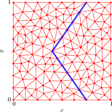
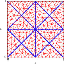
Fig. 1: An unstructured mesh with the interface $\Gamma$ (thick-dashed).

We denote by $H$ the maximum diameter of the subdomains and by $H_{\Omega}$ the diameter of the mono-domain $\Omega$. We assume $0<h\leq H<H_{\Omega}$.

We introduce local spaces on $\Omega_{1}$ and $\Omega_{2}$ by

(11) $$V_{h,i}:=\big{\{}v\in\textrm{L}^{2}(\Omega_{i}):\left.v\right|_{K\in\mathcal{T}_{i}}\in\mathbb{P}^{k}(K)\big{\}},\text{ for }i=1,2.$$

Note that this domain decomposition setting implies $V_{h}=V_{h,1}\oplus V_{h,2}$. We define on the interface the space of broken single-valued functions by

(12) $$\Lambda_{h}:=\big{\{}\varphi\in\textrm{L}^{2}(\Gamma):\left.\varphi\right|_{e\in\Gamma}\in\mathbb{P}^{k}(e)\big{\}}.$$

For the sake of simplicity we denote the restriction of $v\in V_{h}$ on $V_{h,i}$ by $v_{i}$. Observe that the trace of $v_{i}\in V_{h,i}$ on $\Gamma$ belongs to $\Lambda_{h}$.

Let $(u,\lambda),(v,\varphi)\in V_{h}\times\Lambda_{h}$ and consider the symmetric bilinear form

(13) $$\tilde{a}((u,\lambda),(v,\varphi)):=\tilde{a}_{\Gamma}(\lambda,\varphi)+\sum_{i=1}^{2}\Big{(}\tilde{a}_{i}(u_{i},v_{i})+\tilde{a}_{i\Gamma}(v_{i},\lambda)+\tilde{a}_{i\Gamma}(u_{i},\varphi)\Big{)},$$

where

(14) $$\begin{array}[]{rcl}\tilde{a}_{\Gamma}(\lambda,\varphi)&:=&2\left\langle\mu\,\lambda,\varphi\right\rangle_{\Gamma},\\ \tilde{a}_{i\Gamma}(v_{i},\varphi)&:=&\left\langle\frac{\partial{v_{i}}}{\partial{{\boldsymbol{n}}_{i}}}-\mu v_{i},\varphi\right\rangle_{\Gamma},\end{array}$$

and

(15) $$\begin{array}[]{rcl}\tilde{a}_{i}(u_{i},v_{i})&:=&\eta\left({u_{i}},{v_{i}}\right)_{\mathcal{T}_{i}}+\left({\nabla u_{i}},{\nabla v_{i}}\right)_{\mathcal{T}_{i}}-\left\langle\{\!\!\{\nabla u_{i}\}\!\!\},[\![v_{i}]\!]\right\rangle_{\mathcal{E}_{i}^{0}}-\left\langle\{\!\!\{\nabla v_{i}\}\!\!\},[\![u_{i}]\!]\right\rangle_{\mathcal{E}_{i}^{0}}\\ &&+\left\langle\frac{\mu}{2}[\![u_{i}]\!],[\![v_{i}]\!]\right\rangle_{\mathcal{E}_{i}^{0}}-\left\langle\frac{1}{2\mu}[\![\nabla u_{i}]\!],[\![\nabla v_{i}]\!]\right\rangle_{\mathcal{E}_{i}^{0}}\\ &&-\left\langle\frac{\partial{u_{i}}}{\partial{{\boldsymbol{n}}_{i}}},v_{i}\right\rangle_{\partial\Omega_{i}}-\left\langle\frac{\partial{v_{i}}}{\partial{{\boldsymbol{n}}_{i}}},u_{i}\right\rangle_{\partial\Omega_{i}}+\left\langle{\mu}\,{u_{i}},{v_{i}}\right\rangle_{\partial\Omega_{i}}.\end{array}$$

This is an IPH discretization of the model problem in $\Omega_{i}$ and $\partial\Omega_{i}$ is treated as a Dirichlet boundary. Therefore $\tilde{a}_{i}(\cdot,\cdot)$ inherits coercivity and continuity of the original bilinear form, $a(\cdot,\cdot)$.

The global bilinear form $\tilde{a}(\cdot,\cdot)$ is also coercive at the discrete level, if $\alpha>0$ is sufficiently large, independent of $h$. To see this we introduce an energy norm for all $(v_{i},\varphi)\in V_{h,i}\times\Lambda_{h}$ such that

(16) $$\|{(v_{i},\varphi)}\|_{{\tt HDG},i}^{2}:=\eta{\|v_{i}\|}_{\mathcal{T}_{i}}^{2}+{\|\nabla v_{i}\|}_{\mathcal{T}_{i}}^{2}+\mu{\|[\![v_{i}]\!]\|}_{\mathcal{E}_{i}\setminus\Gamma}^{2}+\mu{\|v_{i}-\varphi\|}_{\Gamma}^{2},\quad(i=1,2).$$

then by definition of $\tilde{a}(\cdot,\cdot)$ for all $(v,\varphi)\in V_{h}\times\Lambda_{h}$ we have

(17) $$\begin{array}[]{rcl}\tilde{a}((v,\varphi),(v,\varphi))&=&\tilde{a}_{\Gamma}(\varphi,\varphi)+\sum_{i=1}^{2}\big{(}\tilde{a}_{i}(v_{i},v_{i})+2\tilde{a}_{i\Gamma}(v_{i},\varphi)\big{)},\\ &=&\sum_{i=1}^{2}\big{(}\tilde{a}_{i}(v_{i},v_{i})+2\tilde{a}_{i\Gamma}(v_{i},\varphi)+\frac{1}{2}\tilde{a}_{\Gamma}(\varphi,\varphi)\big{)}.\end{array}$$

We can bound the contribution of each subdomain from below separately:

$$\begin{array}[]{rcl}\tilde{a}((v,\varphi),(v,\varphi))&=&\sum_{i=1}^{2}\eta\|v_{i}\|_{\mathcal{T}_{i}}^{2}+\|\nabla v_{i}\|_{\mathcal{T}_{i}}^{2}\\ &&\quad-2\left\langle\{\!\!\{\nabla v_{i}\}\!\!\},[\![v_{i}]\!]\right\rangle_{\mathcal{E}_{i}\setminus\Gamma}+\frac{\mu}{2}\|[\![v_{i}]\!]\|_{\mathcal{E}_{i}\setminus\Gamma}^{2}-\frac{1}{2\mu}\|[\![\nabla v_{i}]\!]\|_{\mathcal{E}_{i}^{0}}^{2}\\ &&\quad-2\left\langle\frac{\partial{v_{i}}}{\partial{{\boldsymbol{n}}_{i}}},v_{i}-\varphi\right\rangle_{\Gamma}+\mu\|v_{i}-\varphi\|_{\Gamma}^{2},\\ &\geq&c\sum_{i=1}^{2}\|{(v_{i},\varphi)}\|_{{\tt HDG},i}^{2},\end{array}$$

where we used the inverse inequalities (9) for terms acting on the interface and (8) for terms acting inside subdomains. Here $0<c<1$ is a constant independent of $h$. Note that we proved the coercivity in a subdomain by subdomain fashion by splitting the $\tilde{a}_{\Gamma}(\cdot,\cdot)$ terms.

Consider the following discrete problem: find $(u_{h},\lambda_{h})\in V_{h}\times\Lambda_{h}$ such that

(18) $$\tilde{a}((u_{h},\lambda_{h}),(v,\varphi))=\left({f},{v}\right)_{\mathcal{T}_{h}},\quad\forall(v,\varphi)\in V_{h}\times\Lambda_{h},$$

which has a unique solution since $\tilde{a}(\cdot,\cdot)$ is coercive on $V_{h}\times\Lambda_{h}$. One can eliminate the interface variable, $\lambda_{h}$, and obtain a variational problem in terms of $u_{h}$ only. It turns out that this coincides with the variational problem (10); for a proof see [21].

The advantage of the variational problem (18) is that each subproblem is communicating through the auxiliary unknown $\lambda_{h}$. Therefore we can eliminate the interior unknowns, $u_{i}$, and obtain a Schur complement system. If we test (18) with $v_{i}\not=0$, $v_{j}=0$ $(j\not=i)$, $\varphi=0$ and assume that $\lambda_{h}$ is known, we obtain a local problem: find $u_{i}\in V_{h,i}$ such that

(19) $$\tilde{a}_{i}(u_{i},v_{i})+\tilde{a}_{i\Gamma}(v_{i},\lambda_{h})=\left({f},{v_{i}}\right)_{\mathcal{T}_{i}},\quad\forall v_{i}\in V_{h,i}.$$

This is an IPH discretization of the continuous problem

$$\begin{array}[]{rcll}(\eta-\Delta)u&=&f,&\text{in $\Omega_{i}$},\\ u&=&\lambda_{h},&\text{on $\Gamma$},\\ u&=&0,&\text{on $\partial\Omega_{i}\setminus\Gamma$}.\end{array}$$

However the boundary condition on $\Gamma$ is imposed weakly and therefore $u_{i}|_{\Gamma}\not=\lambda_{h}$ in the strong sense, see [7, 15, 21].

2.4 Schur complement formulation

We choose nodal basis functions for $\mathbb{P}^{k}(K)$ and denote the space of degrees of freedom (DOFs) of $V_{h}$ by $V$ and similarly for subspaces by $\{V_{i}\}$. The variational form in (10) is equivalent to the linear system $A{\boldsymbol{u}}={\boldsymbol{f}}$. $A$ is the system matrix and ${\boldsymbol{u}}\in V$ are the corresponding DOFs of the approximation $u_{h}\in V_{h}$. We can partition ${\boldsymbol{u}}$ into $\{{\boldsymbol{u}}_{i}\}$ where ${\boldsymbol{u}}_{i}$ corresponds to DOFs of $u_{i}\in V_{h,i}$. Then we can arrange the entries of $A$ and rewrite the linear system as

(20) $$\left[\begin{array}[]{cc}{A_{1}}&{A_{12}}\\ {A_{21}}&{A_{2}}\end{array}\right]\left(\begin{array}[]{c}{{\boldsymbol{u}}_{1}}\\ {{\boldsymbol{u}}_{2}}\end{array}\right)=\left(\begin{array}[]{c}{{\boldsymbol{f}}_{1}}\\ {{\boldsymbol{f}}_{2}}\end{array}\right).$$

We use nodal basis functions for $\Lambda_{h}$ and denote by ${\boldsymbol{\lambda}}$ the corresponding DOFs for $\lambda_{h}\in\Lambda_{h}$. Then the variational form (18) can be written as

(21) $$\left[\begin{array}[]{ccc}{\tilde{A}_{1}}&{}\hfil&{\tilde{A}_{1\Gamma}}\\ {}\hfil&{\tilde{A}_{2}}&{\tilde{A}_{2\Gamma}}\\ {\tilde{A}_{\Gamma 1}}&{\tilde{A}_{\Gamma 2}}&{\tilde{A}_{\Gamma}}\end{array}\right]\left(\begin{array}[]{c}{{\boldsymbol{u}}_{1}}\\ {{\boldsymbol{u}}_{2}}\\ {{\boldsymbol{\lambda}}}\end{array}\right)=\left(\begin{array}[]{c}{{\boldsymbol{f}}_{1}}\\ {{\boldsymbol{f}}_{2}}\\ {0}\end{array}\right),$$

where $\tilde{A}_{\Gamma i}=\tilde{A}_{i\Gamma}^{\top}$. Since this matrix is s.p.d. and the same holds also for its diagonal blocks, we can form a Schur complement system. We define $\tilde{B}_{i}:=\tilde{A}_{\Gamma i}\tilde{A}_{i}^{-1}\tilde{A}_{i\Gamma}$ and ${\boldsymbol{g}}_{\Gamma}:=-\sum_{i=1}^{2}\tilde{A}_{\Gamma i}\tilde{A}_{i}^{-1}{\boldsymbol{f}}_{i}.$ Then the Schur complement system reads

(22) $$\tilde{S}_{\Gamma}{\boldsymbol{\lambda}}:=\Big{(}\tilde{A}_{\Gamma}-\sum_{i=1}^{2}\tilde{B}_{i}\Big{)}{\boldsymbol{\lambda}}={\boldsymbol{g}}_{\Gamma}.$$

Definition 3 (discrete harmonic extension).

For all $\varphi\in\Lambda_{h}$, we denote by $\mathcal{H}_{i}(\varphi)\in V_{h,i}$ the discrete harmonic extension into $\Omega_{i}$,

(23) $$\mathcal{H}_{i}(\varphi)\equiv-\tilde{A}_{i}^{-1}\tilde{A}_{i\Gamma}{\boldsymbol{\varphi}}.$$

The corresponding $\varphi$ is called generator. In other words $u_{i}:=\mathcal{H}_{i}(\varphi)$ is an approximation obtained from the IPH discretization in $\Omega_{i}$ using $\varphi$ as Dirichlet data; i.e. $\tilde{A}_{i}{\boldsymbol{u}}_{i}+\tilde{A}_{i\Gamma}{\boldsymbol{\varphi}}=0$.

The following result shows that an application of $\tilde{B}_{i}{\boldsymbol{\lambda}}$ can be viewed as finding the harmonic extension, $u_{i}:=\mathcal{H}_{i}(\lambda_{h})$, and then evaluating a “Robin-like trace” on the interface.

Proposition 4.

Let $\lambda_{h}\in\Lambda_{h}$ and define its harmonic extension by $u_{i}:=\mathcal{H}_{i}(\lambda_{h})$. Then ${\boldsymbol{\varphi}}^{\top}\tilde{B}_{i}{\boldsymbol{\lambda}}=\left\langle\mu u_{i}-\frac{\partial{u_{i}}}{\partial{{\boldsymbol{n}}_{i}}},\varphi\right\rangle_{\Gamma}$ for all $\varphi\in\Lambda_{h}$.

Proof.

Let $u_{i}:=\mathcal{H}_{i}(\lambda_{h})$. Then by definition of $\tilde{B}_{i}$ and $\tilde{a}_{i\Gamma}(\cdot,\cdot)$ we have

$${\boldsymbol{\varphi}}^{\top}\tilde{B}_{i}{\boldsymbol{\lambda}}={\boldsymbol{\varphi}}^{\top}\tilde{A}_{\Gamma i}\tilde{A}_{i}^{-1}\tilde{A}_{i\Gamma}{\boldsymbol{\lambda}}=-{\boldsymbol{\varphi}}^{\top}\tilde{A}_{\Gamma i}{\boldsymbol{u}}_{i}=\left\langle\mu u_{i}-\frac{\partial{u_{i}}}{\partial{{\boldsymbol{n}}_{i}}},\varphi\right\rangle_{\Gamma},$$

for all $\varphi\in\Lambda_{h}$, which completes the proof, since $\tilde{A}_{\Gamma i}=\tilde{A}_{i\Gamma}^{\top}$.  ∎

3 Properties of the Schur complement and technical tools

The main goal of this section is to provide estimates for the minimum and maximum eigenvalues of the $\tilde{S}_{\Gamma}$ and $\tilde{B}_{i}$ for $i=1,2$. We use the estimate for the $\tilde{B}_{i}$ operators to prove convergence of the Schwarz method and provide the contraction factor later in Section 4. In particular we prove in this section that the following estimates hold for all $\varphi\in\Lambda_{h}$:

(24) $$c_{B}\,\mu\|\varphi\|_{\Gamma}^{2} \leq{\boldsymbol{\varphi}}^{\top}\tilde{B}_{i}{\boldsymbol{\varphi}}\leq \Big{(}1-C_{B}\frac{h}{H\alpha}\Big{)}\mu\|\varphi\|_{\Gamma}^{2},$$

(25) $$c\frac{H}{H_{\Omega}^{2}}\|\varphi\|_{\Gamma}^{2} \leq{\boldsymbol{\varphi}}^{\top}\tilde{S}_{\Gamma}{\boldsymbol{\varphi}}\leq C\frac{\alpha}{h}\|\varphi\|_{\Gamma}^{2},$$

where all constants are positive and independent of $h$, $H$ and $H_{\Omega}$. Since $\tilde{S}_{\Gamma}$ and $\tilde{B}_{i}$ are symmetric, we can use Rayleigh quotient arguments and obtain an estimate for the minimum and maximum eigenvalues. One can also obtain an estimate with polynomial degree dependency using the techniques of this section.

The only constraint on the shape of the subdomains is a star-shape assumption. To prove the above estimates we need trace and Poincaré inequalities for totally discontinuous functions. The following trace estimate is due to Feng and Karakashian [12, Lemma 3.1]. The Poincaré inequality is due to Brenner, see [5].

Lemma 5 (Trace inequality).

Let $D$ be a star-shape domain with diameter $H_{D}$, and triangulation $\mathcal{T}_{h}$. Then, for any $u\in{\textrm{H}}^{1}(\mathcal{T}_{h})$, we have

$$\|u\|_{\partial D}^{2}\leq c\Big{[}H_{D}^{-1}\|u\|_{D}^{2}+H_{D}\big{(}\|\nabla u\|_{D}^{2}+h^{-1}\|[\![u]\!]\|_{\mathcal{E}\setminus\partial D}^{2}\big{)}\Big{]}.$$

Lemma 6 (Poincaré inequality).

Let $D$ be an open connected polygonal domain with diameter $H_{D}$, and triangulation $\mathcal{T}_{h}$. Then, for any $u\in{\textrm{H}}^{1}(\mathcal{T}_{h})$ we have

$$\|u\|_{D}^{2}\leq cH_{D}^{2}\Big{[}\|\nabla u\|_{D}^{2}+h^{-1}\|[\![u]\!]\|_{\mathcal{E}\setminus\partial D}^{2}+h^{-1}\|{u}\|_{\nu}^{2}\Big{]},$$

where $\nu$ is a measurable subset of $\partial D$ with nonzero measure.

3.1 Eigenvalue estimates for $\tilde{B}_{i}$

In order to obtain estimates for the eigenvalues of the $\tilde{B}_{i}$ operator, we first recall Definition 3 of a harmonic extension: $u_{i}\in V_{h,i}$ is called harmonic extension of $\varphi\in\Lambda_{h}$ if it satisfies $\tilde{A}_{i}{\boldsymbol{u}}_{i}+\tilde{A}_{i\Gamma}{\boldsymbol{\varphi}}=0$. Now multiplying this relation by ${\boldsymbol{u}}_{i}^{\top}$ from left we get

$$\begin{array}[]{llcl}&{\boldsymbol{u}}_{i}^{\top}\tilde{A}_{i}{\boldsymbol{u}}_{i}+{\boldsymbol{u}}_{i}^{\top}\tilde{A}_{i\Gamma}{\boldsymbol{\varphi}}&=&0\\ \Leftrightarrow&{\boldsymbol{u}}_{i}^{\top}\tilde{A}_{i}{\boldsymbol{u}}_{i}-{\boldsymbol{\varphi}}^{\top}\tilde{A}_{\Gamma i}\tilde{A}_{i}^{-1}\tilde{A}_{i\Gamma}{\boldsymbol{\varphi}}&=&0\\ \Leftrightarrow&{\boldsymbol{u}}_{i}^{\top}\tilde{A}_{i}{\boldsymbol{u}}_{i}-{\boldsymbol{\varphi}}^{\top}\tilde{B}_{i}{\boldsymbol{\varphi}}&=&0,\end{array}$$

where we used ${\boldsymbol{u}}_{i}=-\tilde{A}_{i}^{-1}\tilde{A}_{i\Gamma}{\boldsymbol{\varphi}}$, $\tilde{A}_{\Gamma i}=\tilde{A}_{i\Gamma}^{\top}$ and the definition of $\tilde{B}_{i}$. Hence if $u_{i}=\mathcal{H}_{i}(\varphi)$ then we have

(26) $${\boldsymbol{\varphi}}^{\top}\tilde{B}_{i}{\boldsymbol{\varphi}}=\tilde{a}_{i}(u_{i},u_{i}).$$

Now recall that $\tilde{a}_{i}(\cdot,\cdot)$ is coercive and bounded over $V_{h,i}$, therefore $\underline{c}\|{u_{i}}\|_{\textrm{\tt DG}{}}^{2}\leq\tilde{a}_{i}(u_{i},u_{i})\leq\overline{C}\|{u_{i}}\|_{\textrm{\tt DG}{}}^{2}$. Thus if we relate the energy norm of the harmonic extension, $u_{i}:=\mathcal{H}_{i}(\varphi)\in V_{h,i}$, to the $\textrm{L}^{2}$-norm of $\varphi$ we obtain the desired estimate (24). More precisely we can show that the estimate

(27) $${c}_{\mathcal{H}}\cdot\mu\|\varphi\|_{\Gamma}^{2}\leq\|{u_{i}}\|_{\textrm{\tt DG}{}}^{2}\leq{C}_{\mathcal{H}}\cdot\mu\|\varphi\|_{\Gamma}^{2}$$

holds, where $0<c_{\mathcal{H}}<1$ and $C_{\mathcal{H}}>1$ are constants independent of $h$. Observe that $C_{\mathcal{H}}>1$ while the upper bound estimate in (24) is less than one. We show later how one can obtain a sharp upper bound estimate as in (24).

Let us start with the lower bound of inequality (27). First we introduce an extension by zero operator ${\boldsymbol{\theta}}_{i}:\Lambda_{h}\rightarrow V_{h,i}$ which is defined for all $\varphi\in\Lambda_{h}$ as

$${\boldsymbol{\theta}}_{i}(\varphi):=\left\{\begin{array}[]{ll}\varphi&\text{on edges belonging to $\Gamma$},\\ 0&\text{on other nodes}.\end{array}\right.$$

For a graphical illustration see Figure 2.

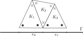
Fig. 2: Illustration of the extension by zero, ${\boldsymbol{\theta}}_{i}(\varphi)$, for elements which share an edge with the interface, e.g. $\{K_{1},K_{3}\}$, and those which do not, e.g. $K_{2}$.

Note that there are elements like $K_{2}$ which physically share a node and not an edge with the interface, but we leave ${\boldsymbol{\theta}}_{i}(\varphi)$ in $K_{2}$ to be zero. More precisely, only those elements which share an edge with the interface are non-zero.

We show in the Appendix, see also [23], that in an element, $K\in\mathcal{T}_{i}$, with an edge $e\in\Gamma$ we have

(28) $$\begin{array}[]{lcl}\|{\boldsymbol{\theta}}_{i}(\varphi)\|_{K}^{2}&\leq&C_{3}\,h\|\varphi\|_{e}^{2},\\ \|\nabla{\boldsymbol{\theta}}_{i}(\varphi)\|_{K}^{2}&\leq&{C_{4}}{h^{-1}}\|\varphi\|_{e}^{2},\\ \|[\![{\boldsymbol{\theta}}_{i}(\varphi)]\!]\|_{\mathcal{E}_{i}}^{2}&\leq&C_{5}\|\varphi\|_{\Gamma}^{2},\end{array}$$

where $C_{3}>0$, $C_{4}>0$ and $C_{5}\geq 1$ and all are independent of $h$. This yields the following result which relates the energy of the extension by zero to its $\textrm{L}^{2}$-norm on the interface.

Lemma 7.

Let $\varphi\in\Lambda_{h}$ and ${\boldsymbol{\theta}}_{i}(\varphi)$ be its extension by zero into $\Omega_{i}$. We have

$$\|{{\boldsymbol{\theta}}_{i}(\varphi)}\|_{\textrm{\tt DG}{}}^{2}\leq\mu\,C_{\theta}\,\|\varphi\|_{\Gamma}^{2},$$

where $C_{\theta}=C_{3}\eta+C_{4}\alpha^{-1}+C_{5}>1$.

Proof.

First note that by definition ${\boldsymbol{\theta}}_{i}(\varphi)$ and $\nabla{\boldsymbol{\theta}}_{i}(\varphi)$ are non-zero only on those elements which share an edge with the interface. We call them $\{K_{\Gamma}\}\subset\mathcal{T}_{i}$. Then we have

$$\begin{array}[]{rcll}\|{{\boldsymbol{\theta}}_{i}(\varphi)}\|_{\textrm{\tt DG}{}}^{2}&=&\displaystyle\sum_{K\in\{K_{\Gamma}\}}\eta\|{\boldsymbol{\theta}}_{i}(\varphi)\|_{K}^{2}+\|\nabla{\boldsymbol{\theta}}_{i}(\varphi)\|_{K}^{2}+\mu\|[\![{\boldsymbol{\theta}}_{i}(\varphi)]\!]\|_{\mathcal{E}_{i}}^{2}\\ &\leq&C_{3}\,\eta\,h\|\varphi\|_{\Gamma}^{2}+\frac{C_{4}}{{h}}\|\varphi\|_{\Gamma}^{2}+C_{5}\,\mu\|\varphi\|_{\Gamma}^{2}\\ &\leq&\mu\left(C_{3}\,\eta+\frac{C_{4}}{\alpha}+C_{5}\right)\|\varphi\|_{\Gamma}^{2},\end{array}$$

which completes the proof with $C_{\theta}:=C_{3}\,\eta+\frac{C_{4}}{\alpha}+C_{5}>1$.  ∎

Now we are able to relate the energy of a harmonic extension, $u_{i}:=\mathcal{H}_{i}(\varphi)$, to the $\textrm{L}^{2}$-norm of $\varphi$ on the interface.

Lemma 8.

Let $\varphi\in\Lambda_{h}$ and $u_{i}:=\mathcal{H}_{i}(\varphi)$ be its harmonic extension into $\Omega_{i}$. Then we have

$${c}_{\mathcal{H}}\cdot\mu\|\varphi\|_{\Gamma}^{2}\leq\|{u_{i}}\|_{\textrm{\tt DG}{}}^{2},$$

where $c_{\mathcal{H}}=(1-\frac{c}{\alpha})^{2}\cdot\frac{1}{C_{\theta}\overline{C}^{2}}<1$.

Proof.

Since $u_{i}$ is the harmonic extension of $\varphi$, it satisfies (19) (with $f=0$). Let $v={\boldsymbol{\theta}}_{i}(\varphi)$. Then by definition of $\tilde{a}_{i\Gamma}(\cdot,\cdot)$ we have

$$\tilde{a}_{i}(u_{i},{\boldsymbol{\theta}}_{i}(\varphi))=\left\langle\mu\,{\boldsymbol{\theta}}_{i}(\varphi)-\frac{\partial{{\boldsymbol{\theta}}_{i}(\varphi)}}{\partial{{\boldsymbol{n}}_{i}}},\varphi\right\rangle_{\Gamma}.$$

Note that ${\boldsymbol{\theta}}_{i}(\varphi)|_{\Gamma}=\varphi$. We can bound the right-hand side from below, therefore

$$\begin{array}[]{rcll}\tilde{a}_{i}(u_{i},{\boldsymbol{\theta}}_{i}(\varphi))&\geq&\mu\|\varphi\|_{\Gamma}^{2}-\|\frac{\partial{{\boldsymbol{\theta}}_{i}(\varphi)}}{\partial{{\boldsymbol{n}}_{i}}}\|_{\Gamma}\,\|\varphi\|_{\Gamma}&\\ &\geq&\mu\|\varphi\|_{\Gamma}^{2}-\frac{c}{\sqrt{h}}\|\nabla{{\boldsymbol{\theta}}_{i}(\varphi)}\|_{K_{\Gamma}}\,\|\varphi\|_{\Gamma}&\quad\textrm{by ineq.~{}(\ref{eq:warburton})}\\ &\geq&\mu\|\varphi\|_{\Gamma}^{2}-\frac{c^{\prime}}{h}\,\|\varphi\|_{\Gamma}^{2}&\quad\textrm{by ineq.~{}(\ref{eq:zoptineq})}\\ &=&\mu\left(1-\frac{c^{\prime}}{\alpha}\right)\|\varphi\|_{\Gamma}^{2},\end{array}$$

which is positive if $\alpha>0$ and sufficiently large. By continuity of $\tilde{a}_{i}(\cdot,\cdot)$ we have

$$\mu\left(1-\frac{c^{\prime}}{\alpha}\right)\|\varphi\|_{\Gamma}^{2}\leq\overline{C}\,\|{u_{i}}\|_{\textrm{\tt DG}{}}\cdot\|{{\boldsymbol{\theta}}_{i}(\varphi)}\|_{\textrm{\tt DG}{}}.$$

Note that we are able to use $\|{\cdot}\|_{\textrm{\tt DG}{}}$ instead of $\|{\cdot}\|_{\textrm{\tt DG}{,\ast}}$ since we work with discrete spaces. An application of Lemma 7 completes the proof with $c_{\mathcal{H}}=(1-\frac{c^{\prime}}{\alpha})^{2}\cdot\frac{1}{C_{\theta}\overline{C}^{2}}<1$.  ∎

The upper bound in (27) can be obtained much easier using coercivity of the $\tilde{a}_{i}(\cdot,\cdot)$.

Lemma 9.

Let $\varphi\in\Lambda_{h}$ and $u_{i}:=\mathcal{H}_{i}(\varphi)$ be its harmonic extension into $\Omega_{i}$. Then we have

$$\|{u_{i}}\|_{\textrm{\tt DG}{}}^{2}\leq{C}_{\mathcal{H}}\cdot\mu\|\varphi\|_{\Gamma}^{2},$$

where $C_{\mathcal{H}}=\left(1+\frac{C}{\sqrt{\alpha}}\right)^{2}\cdot\frac{1}{\underline{c}^{2}}>1$.

Proof.

Since $u_{i}$ is the harmonic extension of $\varphi$, it satisfies (19) (with $f=0$). Using the fact that $\tilde{a}_{i}(\cdot,\cdot)$ is coercive we have

$$\begin{array}[]{rcl}\underline{c}\|{u_{i}}\|_{\textrm{\tt DG}{}}^{2}\leq\tilde{a}_{i}(u_{i},u_{i})&=&-\tilde{a}_{i\Gamma}(u_{i},\varphi)\\ &=&\left\langle\mu u_{i}-\frac{\partial{u_{i}}}{\partial{{\boldsymbol{n}}_{i}}},\varphi\right\rangle_{\Gamma}\\ &\leq&\mu\|u_{i}\|_{\Gamma}\|\varphi\|_{\Gamma}+\|\frac{\partial{u_{i}}}{\partial{{\boldsymbol{n}}_{i}}}\|_{\Gamma}\|\varphi\|_{\Gamma}\\ &\leq&\mu\|u_{i}\|_{\Gamma}\|\varphi\|_{\Gamma}+\frac{C}{\sqrt{h}}\|\nabla u_{i}\|_{\mathcal{T}_{i}}\|\varphi\|_{\Gamma}\\ &\leq&\mu^{\frac{1}{2}}\left(1+\frac{C}{\sqrt{\alpha}}\right)\|{u_{i}}\|_{\textrm{\tt DG}{}}\cdot\|\varphi\|_{\Gamma},\end{array}$$

which completes the proof with $C_{\mathcal{H}}:=\left(1+\frac{C}{\sqrt{\alpha}}\right)^{2}\cdot\frac{1}{\underline{c}^{2}}>1$.  ∎

We see that $C_{\mathcal{H}}>1$, which does not provide a sharp estimate for the maximum eigenvalue of $\tilde{B}_{i}$. We now show how to obtain a sharp estimate for the maximum eigenvalue of the $\tilde{B}_{i}$. Recall that the global matrix $\tilde{A}$ is s.p.d. and the positive definiteness is proved by using for each subdomain $\frac{1}{2}\tilde{A}_{\Gamma}$ in (17). Therefore we consider the s.p.d. matrix

$$\hat{A}:=\left[\begin{array}[]{cc}{\tilde{A}_{i}}&{\tilde{A}_{i\Gamma}}\\ {\tilde{A}_{\Gamma i}}&{\frac{1}{2}\tilde{A}_{\Gamma}}\end{array}\right].$$

To show positive-definiteness, let ${\boldsymbol{w}}:=({\boldsymbol{u}}_{i},{\boldsymbol{\varphi}})^{\top}$ and observe

(29) $${\boldsymbol{w}}^{\top}\hat{A}{\boldsymbol{w}}=\tilde{a}_{i}(u_{i},u_{i})+2\tilde{a}_{i\Gamma}(u_{i},\varphi)+\frac{1}{2}\tilde{a}_{\Gamma}(\varphi,\varphi)\geq c\|{(u_{i},\varphi)}\|_{{\tt HDG},i}^{2},$$

for all $u_{i}\in V_{h,i}$ and $\varphi\in\Lambda_{h}$. Now let $u_{i}=\mathcal{H}_{i}(\varphi)$, then by a simple manipulation we have ${\boldsymbol{\varphi}}^{\top}\big{(}\frac{1}{2}\tilde{A}_{\Gamma}-\tilde{B}_{i}\big{)}{\boldsymbol{\varphi}}={\boldsymbol{w}}^{\top}\hat{A}{\boldsymbol{w}}$. Combining with (29) and recalling that ${\boldsymbol{\varphi}}^{\top}\tilde{A}_{\Gamma}{\boldsymbol{\varphi}}=2\mu\|\varphi\|^{2}_{\Gamma}$ we obtain

(30) $$\mu\|\varphi\|_{\Gamma}^{2}-c\|{(\mathcal{H}_{i}(\varphi),\varphi)}\|_{{\tt HDG},i}^{2}\geq{\boldsymbol{\varphi}}^{\top}\tilde{B}_{i}{\boldsymbol{\varphi}}.$$

This gives a sharp estimate for the maximum eigenvalue of $\tilde{B}_{i}$ if we can bound the second term from below which is stated in the following lemma.

Lemma 10.

Let $\varphi\in\Lambda_{h}$ and $u_{i}\in V_{h,i}$ for $i=1,2$. Let $H_{i}$ be the diameter of the subdomain. Then we have

$$\frac{c}{H_{i}}\|\varphi\|_{\Gamma}^{2}\leq\|{(u_{i},\varphi)}\|_{{\tt HDG},i}^{2}.$$

Proof.

We first invoke triangle inequality and then Young’s inequality

$$\|\varphi\|_{\Gamma}^{2}\leq\|u_{i}-\varphi\|_{\Gamma}^{2}+\|u_{i}\|_{\Gamma}^{2}\leq{H_{i}}h^{-1}\|u_{i}-\varphi\|_{\Gamma}^{2}+\|u_{i}\|_{\Gamma}^{2},$$

where the last inequality is due to the fact that $h\leq{H_{i}}$. Now for the second term on the right-hand side we apply the trace inequality from Lemma 5, and subsequently the Poincaré inequality from Lemma 6 with $\nu=\partial\Omega_{i}\setminus\Gamma$. We obtain

$$\begin{array}[]{rcl}\|\varphi\|_{\Gamma}^{2}&\leq&{H_{i}}h^{-1}\|u_{i}-\varphi\|_{\Gamma}^{2}+c_{1}H_{i}\big{(}\|\nabla u_{i}\|_{\Omega_{i}}^{2}+h^{-1}\|[\![u_{i}]\!]\|_{\mathcal{E}_{i}\setminus\Gamma}^{2}\big{)}\\ &\leq&c_{2}H_{i}\|{(u_{i},\varphi)}\|_{{\tt HDG},i}^{2},\end{array}$$

which completes the proof.  ∎

We are now in the position to prove the estimate for the eigenvalues of $\tilde{B}_{i}$.

Lemma 11.

There exists $\alpha>0$, sufficiently large, such that

$$c_{B}\mu\|\varphi\|_{\Gamma}^{2}\leq{\boldsymbol{\varphi}}^{\top}\tilde{B}_{i}{\boldsymbol{\varphi}}\leq\Big{(}1-C_{B}\frac{h}{H\alpha}\Big{)}\mu\|\varphi\|_{\Gamma}^{2},\quad\forall\varphi\in\Lambda_{h},$$

where $0<c_{B}<1$. Therefore $\tilde{B}_{i}$ is s.p.d. Moreover $\tilde{A}_{\Gamma}-2\tilde{B}_{i}$ is s.p.d.

Proof.

To show the proof of the lower bound we use (26), coercivity of $\tilde{a}_{i}(\cdot,\cdot)$ and Lemma 8 to obtain

$${\boldsymbol{\varphi}}^{\top}\tilde{B}_{i}{\boldsymbol{\varphi}}=\tilde{a}_{i}(u_{i},u_{i})\geq\underline{c}\|{u_{i}}\|_{\textrm{\tt DG}{}}^{2}\geq\underline{c}\cdot c_{\mathcal{H}}\cdot\mu\|\varphi\|_{\Gamma}^{2}.$$

This completes the lower bound by setting $c_{B}:=\underline{c}\cdot c_{\mathcal{H}}<1$. For the upper bound we use inequality (30) and Lemma 10 where we obtain

$${\boldsymbol{\varphi}}^{\top}\tilde{B}_{i}{\boldsymbol{\varphi}}\leq\Big{(}1-\frac{c}{H}\frac{h}{\alpha}\Big{)}\mu\|\varphi\|_{\Gamma}^{2}.$$

Finally from inequality (30) we have that $\tilde{A}_{\Gamma}-2\tilde{B}_{i}$ is s.p.d. ∎

Remark 1.

This estimate shows that the condition number satisfies

$$\kappa(\tilde{B}_{i})\leq c_{B}^{-1}\big{(}1-C_{B}\frac{h}{H\alpha}\big{)},$$

which implies that $\tilde{B}_{i}$ is scalable. In other words if we keep the ratio $h/H$ constant the condition number does not change. Geometrically that is equivalent of scaling the subdomain and the triangulation at the same rate which does not change the entries of the $\tilde{B}_{i}$ nor its size. Therefore the condition number of $\tilde{B}_{i}$ is expected not to change.

3.2 Eigenvalue estimate for $\tilde{S}_{\Gamma}$

Estimating eigenvalues of the Schur complement is similar to estimating eigenvalues of $\tilde{B}_{i}$. To show the lower bound in estimate (25), we need the following lemma.

Lemma 12.

Let $\varphi\in\Lambda_{h}$ and $u_{i}\in V_{h,i}$ for $i=1,2$. Let $H_{\Omega}$ be the diameter of the domain and $H$ be the maximum diameter of the subdomains. Then we have

$$c\frac{H}{H_{\Omega}^{2}}\|\varphi\|_{\Gamma}^{2}\leq\sum_{i=1}^{2}\|{(u_{i},\varphi)}\|_{{\tt HDG},i}^{2}.$$

Proof.

First we invoke a triangle inequality

$$H_{i}\|\varphi\|_{\Gamma}^{2}\leq H_{i}\|u_{i}-\varphi\|_{\Gamma}^{2}+H_{i}\|u_{i}\|_{\Gamma}^{2}\leq{H_{i}^{2}}h^{-1}\|u_{i}-\varphi\|_{\Gamma}^{2}+H_{i}\|u_{i}\|_{\Gamma}^{2},$$

where the last inequality is due to the fact that $h\leq{H_{i}}$. Now for the second term on the right-hand side, observe that using Lemma 5 we have

$$c_{i}H_{i}\|u_{i}\|_{\Gamma}^{2}\leq c_{i}H_{i}\|u_{i}\|_{\partial\Omega_{i}}^{2}\leq\|u_{i}\|_{\Omega_{i}}^{2}+H_{i}^{2}\big{(}\|\nabla u_{i}\|_{\Omega_{i}}^{2}+h^{-1}\|[\![u_{i}]\!]\|_{\mathcal{E}_{i}\setminus\partial\Omega_{i}}^{2}\big{)}.$$

We sum over both subdomains and invoke Lemma 6 for the $\textrm{L}^{2}$-norm of $u$ over $\Omega$

$$\begin{array}[]{rcl}cH\sum_{i=1}^{2}\|u_{i}\|_{\Gamma}^{2}&\leq&\|u\|_{\Omega}^{2}+H^{2}\sum_{i=1}^{2}\big{(}\|\nabla u_{i}\|_{\Omega_{i}}^{2}+h^{-1}\|[\![u_{i}]\!]\|_{\mathcal{E}_{i}\setminus\partial\Omega_{i}}^{2}\big{)}\\ &\leq&CH_{\Omega}^{2}\big{(}\|\nabla u\|_{\Omega}^{2}+h^{-1}\|[\![u]\!]\|_{\mathcal{E}\setminus\partial\Omega}^{2}+h^{-1}\|{u}\|_{\partial\Omega}^{2}\big{)}\\ &&\quad+H^{2}\sum_{i=1}^{2}\big{(}\|\nabla u_{i}\|_{\Omega_{i}}^{2}+h^{-1}\|[\![u_{i}]\!]\|_{\mathcal{E}_{i}\setminus\partial\Omega_{i}}^{2}\big{)}.\end{array}$$

Noting that $H\leq H_{\Omega}$ and by definition of $\|{(u_{i},\varphi)}\|_{{\tt HDG},i}$ we obtain

$$\begin{array}[]{rcl}cH\sum_{i=1}^{2}\|u_{i}\|_{\Gamma}^{2}&\leq&H_{\Omega}^{2}\sum_{i=1}^{2}\big{(}\|\nabla u_{i}\|_{\Omega_{i}}^{2}+h^{-1}\|[\![u_{i}]\!]\|_{\mathcal{E}_{i}\setminus\partial\Omega_{i}}^{2}+h^{-1}\|{u_{i}}\|_{\partial\Omega\cap\partial\Omega_{i}}^{2}\big{)}\\ &&+H_{\Omega}^{2}h^{-1}\|[\![u]\!]\|_{\Gamma}^{2}\\ &\leq&H_{\Omega}^{2}\sum_{i=1}^{2}\big{(}\|\nabla u_{i}\|_{\Omega_{i}}^{2}+h^{-1}\|[\![u_{i}]\!]\|_{\mathcal{E}_{i}\setminus\partial\Omega_{i}}^{2}+h^{-1}\|{u_{i}}\|_{\partial\Omega\cap\partial\Omega_{i}}^{2}\big{)}\\ &&+H_{\Omega}^{2}h^{-1}\big{(}\|u_{1}-\varphi\|_{\Gamma}^{2}+\|u_{2}-\varphi\|_{\Gamma}^{2}\big{)}\\ &\leq&H_{\Omega}^{2}\sum_{i=1}^{2}\|{(u_{i},\varphi)}\|_{{\tt HDG},i}^{2}.\end{array}$$

Substituting back into the first inequality completes the proof.  ∎

Lemma 13.

There exists $\alpha>0$, sufficiently large, such that

$$c\frac{H}{H_{\Omega}^{2}}\|\varphi\|_{\Gamma}^{2}\leq{\boldsymbol{\varphi}}^{\top}\tilde{S}_{\Gamma}{\boldsymbol{\varphi}}\leq\frac{2\alpha}{h}\|\varphi\|_{\Gamma}^{2},$$

Therefore $\tilde{S}_{\Gamma}$ is s.p.d. Moreover $\tilde{A}_{\Gamma}-\tilde{B}_{i}$ is s.p.d.

Proof.

The symmetry is easy to check since $\tilde{A}_{\Gamma}$ and $\tilde{B}_{1}$, $\tilde{B}_{2}$ are symmetric. For the upper bound in the estimate we recall that $\tilde{B}_{1}$, $\tilde{B}_{2}$ are positive definite and hence

$${\boldsymbol{\varphi}}^{\top}\tilde{S}_{\Gamma}{\boldsymbol{\varphi}}={\boldsymbol{\varphi}}^{\top}(\tilde{A}_{\Gamma}-\sum_{i=1}^{2}\tilde{B}_{i}){\boldsymbol{\varphi}}\leq{\boldsymbol{\varphi}}^{\top}\tilde{A}_{\Gamma}{\boldsymbol{\varphi}}=2\mu\|\varphi\|_{\Gamma}^{2}.$$

Now let $u_{i}:=\mathcal{H}_{i}(\varphi)$ and ${\boldsymbol{v}}:=({\boldsymbol{u}}_{1},{\boldsymbol{u}}_{2},{\boldsymbol{\varphi}})^{\top}$. A straightforward calculation shows that ${\boldsymbol{\varphi}}^{\top}\tilde{S}_{\Gamma}{\boldsymbol{\varphi}}={\boldsymbol{v}}^{\top}\tilde{A}{\boldsymbol{v}}$. Then the coercivity of the bilinear form $\tilde{a}(\cdot,\cdot)$ and an application of Lemma 12 yields

$${\boldsymbol{\varphi}}^{\top}\tilde{S}_{\Gamma}{\boldsymbol{\varphi}}={\boldsymbol{v}}^{\top}\tilde{A}{\boldsymbol{v}}\equiv\tilde{a}((u,\varphi),(u,\varphi))\geq c\sum_{i=1}^{2}\|{(u_{i},\varphi)}\|_{{\tt HDG},i}^{2}\geq c\frac{H}{H_{\Omega}^{2}}\|\varphi\|_{\Gamma}^{2}.$$

For the final statement, observe that for all $\varphi\not=0$ we have

$${\boldsymbol{\varphi}}^{\top}(\tilde{A}_{\Gamma}-\tilde{B}_{i}){\boldsymbol{\varphi}}>{\boldsymbol{\varphi}}^{\top}(\tilde{A}_{\Gamma}-\sum_{j=1}^{2}\tilde{B}_{j}){\boldsymbol{\varphi}}>0,$$

since the $\{\tilde{B}_{i}\}$ are positive definite. This completes the proof.  ∎

Remark 2.

Note that Lemma 13 provides an upper bound for the condition number, $\kappa(\tilde{S}_{\Gamma})\leq O(\frac{\alpha}{h})$. A similar result also holds for classical FEM, see [4] and [25, Lemma 4.11].

4 Schwarz methods and the Schur complement

In order to solve the Schur complement system we can devise a Schwarz method to obtain $\lambda_{h}$. We will prove that a natural Schwarz method for the Schur complement is equivalent to the block Jacobi iteration in (3), but it suffers from slow convergence. Later we show how to obtain an optimized Schwarz method for the Schur complement which converges much faster to the same fixed point.

Let us relax the constraint that $\lambda_{h}$ is single-valued. Let $\lambda_{h,1},\lambda_{h,2}\in\Lambda_{h}$. Assume $\lambda_{h,2}$ is known; that is we know $u_{2}\in V_{h,2}$. Then we can split the Schur complement system (22) and obtain an approximation for $\lambda_{h,1}$ and consequently $u_{1}\in V_{h,1}$ from

$$(\tilde{A}_{\Gamma}-\tilde{B}_{1}){\boldsymbol{\lambda}}_{1}=\tilde{B}_{2}{\boldsymbol{\lambda}}_{2}+{\boldsymbol{g}}_{\Gamma}.$$

As a consequence of Lemma 13, $(\tilde{A}_{\Gamma}-\tilde{B}_{1})$ is invertible and we can obtain $\lambda_{h,1}$. This suggests an iterative method to obtain $\lambda_{h}$. We will see that this produces identical iterates as the block Jacobi method.

Algorithm 1.

Let $\lambda_{h,1}^{(0)},\lambda_{h,2}^{(0)}\in\Lambda_{h}$ be two random initial guesses. Then for $n=1,2,\ldots$ find $\big{\{}\lambda_{h,i}^{(n)}\big{\}}$ such that

(31) $$\begin{array}[]{rcl}(\tilde{A}_{\Gamma}-\tilde{B}_{1}){\boldsymbol{\lambda}}_{1}^{(n)}=\tilde{B}_{2}{\boldsymbol{\lambda}}_{2}^{(n-1)}+{\boldsymbol{g}}_{\Gamma},\\ (\tilde{A}_{\Gamma}-\tilde{B}_{2}){\boldsymbol{\lambda}}_{2}^{(n)}=\tilde{B}_{1}{\boldsymbol{\lambda}}_{1}^{(n-1)}+{\boldsymbol{g}}_{\Gamma}.\end{array}$$

At convergence, we have $\tilde{A}_{\Gamma}({\boldsymbol{\lambda}}_{1}-{\boldsymbol{\lambda}}_{2})=0$ which implies ${\boldsymbol{\lambda}}_{1}={\boldsymbol{\lambda}}_{2}=\tilde{S}_{\Gamma}^{-1}{\boldsymbol{g}}_{\Gamma}$.

The following result shows that the above method generates the same iterates as the block Jacobi iteration (3). By linearity it suffices to consider the error equation, $f=0$, which implies ${\boldsymbol{g}}_{\Gamma}=0$.

Proposition 14.

Let $\lambda_{h,1}^{(0)},\lambda_{h,2}^{(0)}$ be two random initial guesses of Algorithm 1 and without loss of generality suppose $f=0$. Set the initial guess of the block Jacobi iteration (3) to be $u_{i}^{(0)}=\mathcal{H}_{i}(\lambda_{h,i}^{(0)})$. Then $u_{i}^{(n)}=\mathcal{H}_{i}(\lambda_{h,i}^{(n)})$ for all $n>0$, i.e. both methods produce the same iterates.

Proof.

See [20]. ∎

4.1 Analysis of classical Schwarz for the Schur complement

By linearity we consider the error equations and we denote by ${\boldsymbol{e}}_{i}^{(n)}:={\boldsymbol{\lambda}}_{i}^{(n)}-{\boldsymbol{\lambda}}$. The iterations in (31) can be rewritten in a more suitable form for analysis. Since $\tilde{A}_{\Gamma}$ is s.p.d. (it is just a scaled mass matrix), the square-root $\tilde{A}_{\Gamma}^{1/2}$ exists and is also s.p.d. Therefore, for $i,j\in\{1,2\}$ and $i\not=j$ we can write equivalently

$$\begin{array}[]{lrcl}&(\tilde{A}_{\Gamma}-\tilde{B}_{i}){\boldsymbol{e}}_{i}^{(n)}&=&\tilde{B}_{j}{\boldsymbol{e}}_{j}^{(n-1)}\\ \Leftrightarrow&\tilde{A}_{\Gamma}^{1/2}(I-\tilde{A}_{\Gamma}^{-1/2}\tilde{B}_{i}\tilde{A}_{\Gamma}^{-1/2})\tilde{A}_{\Gamma}^{1/2}{\boldsymbol{e}}_{i}^{(n)}&=&\tilde{B}_{j}{\boldsymbol{e}}_{j}^{(n-1)}\\ \Leftrightarrow&(I-\tilde{A}_{\Gamma}^{-1/2}\tilde{B}_{i}\tilde{A}_{\Gamma}^{-1/2})\tilde{{\boldsymbol{e}}}_{i}^{(n)}&=&(\tilde{A}_{\Gamma}^{-1/2}\tilde{B}_{j}\tilde{A}_{\Gamma}^{-1/2})\tilde{{\boldsymbol{e}}}_{j}^{(n-1)},\end{array}$$

where $\tilde{{\boldsymbol{e}}}_{i}=\tilde{A}_{\Gamma}^{1/2}{\boldsymbol{e}}_{i}$. We define

(32) $$C_{i}:=\tilde{A}_{\Gamma}^{-1/2}\tilde{B}_{i}\tilde{A}_{\Gamma}^{-1/2},$$

which is invertible and symmetric. Since $\tilde{A}_{\Gamma}-\tilde{B}_{i}$ is invertible and $\tilde{A}_{\Gamma}^{1/2}$ exists we can conclude that $I-C_{i}$ is also invertible by definition. Therefore we have

$$(I-C_{i})\tilde{{\boldsymbol{e}}}_{i}^{(n)}=C_{j}\tilde{{\boldsymbol{e}}}_{j}^{(n-1)}=C_{j}(I-C_{j})^{-1}C_{i}\tilde{{\boldsymbol{e}}}_{i}^{(n-2)},$$

or

$${\boldsymbol{\varphi}}_{i}^{(n)}=C_{j}(I-C_{j})^{-1}\cdot C_{i}(I-C_{i})^{-1}{\boldsymbol{\varphi}}_{i}^{(n-2)},$$

where ${\boldsymbol{\varphi}}_{i}=(I-C_{i})\tilde{{\boldsymbol{e}}}_{i}$. Finally the iterations can be rewritten as

(33) $${\boldsymbol{\varphi}}_{i}^{(n)}=(C_{j}^{-1}-I)^{-1}\cdot(C_{i}^{-1}-I)^{-1}{\boldsymbol{\varphi}}_{i}^{(n-2)}.$$

We show how the contraction factor of the iteration in (33) is related to the eigenvalues of $\{C_{i}\}$. Let $\|\cdot\|_{2}$ be the usual 2-norm in $\mathbb{R}^{n}$, and denote by $D_{i}:=(C_{i}^{-1}-I)^{-1}$. Then we can estimate

$$\|{\boldsymbol{\varphi}}_{i}^{(n)}\|_{2}\leq\|D_{j}D_{i}\|_{2}\,\|{\boldsymbol{\varphi}}_{i}^{(n-2)}\|_{2}\leq\|D_{j}\|_{2}\,\|D_{i}\|_{2}\,\|{\boldsymbol{\varphi}}_{i}^{(n-2)}\|_{2}=\rho(D_{j})\,\rho(D_{i})\,\|{\boldsymbol{\varphi}}_{i}^{(n-2)}\|_{2},$$

since $\{D_{i}\}$ are symmetric. In other words we have used a different norm for the error: with $E_{i}:=(I-C_{i})\tilde{A}_{\Gamma}^{1/2}$, which is invertible, we have

$$\|{\boldsymbol{e}}_{i}\|_{E_{i}^{\top}E_{i}}=\|E_{i}{\boldsymbol{e}}_{i}\|_{2}=\|{\boldsymbol{\varphi}}_{i}\|_{2}.$$

Let $\sigma(M)$ denote an eigenvalue of a given matrix $M$. Then we have

$$\rho(D_{i}):=\max_{\sigma(D_{i})}|\sigma(D_{i})|=\max_{\sigma(C_{i})}\left|\frac{\sigma(C_{i})}{1-\sigma(C_{i})}\right|.$$

Hence a sufficient condition for convergence is that $\sigma(C_{i})\in(-\infty,1/2)$. On the other hand by definition of $C_{i}$ we know that $\sigma(C_{i})$ are the eigenvalues of the generalized eigenvalue problem $\tilde{B}_{i}{\boldsymbol{\varphi}}=\sigma\,\tilde{A}_{\Gamma}{\boldsymbol{\varphi}}$. Since both $\tilde{A}_{\Gamma}$ and $\tilde{B}_{i}$ are s.p.d., $\sigma(C_{i})$ is positive. Therefore a sufficient condition for convergence is to show that $\sigma(C_{i})\in(0,1/2)$.

Recall that since $C_{i}$ is symmetric we have

(34) $$\sigma_{\text{min}}(C_{i})=\inf_{{\boldsymbol{\varphi}}\not=0}\frac{{\boldsymbol{\varphi}}^{\top}\tilde{B}_{i}{\boldsymbol{\varphi}}}{{\boldsymbol{\varphi}}^{\top}\tilde{A}_{\Gamma}{\boldsymbol{\varphi}}}=\inf_{{\boldsymbol{\varphi}}\not=0}\frac{{\boldsymbol{\varphi}}^{\top}\tilde{B}_{i}{\boldsymbol{\varphi}}}{2\mu\|\varphi\|_{\Gamma}^{2}}\geq\frac{c_{B}}{2},$$

where we have used the lower bound estimate of Lemma 11. Here $0<c_{B}<1$. The upper bound for $\sigma_{\max}(C_{i})$ can also be obtained using Lemma 11. Hence

(35) $$\sigma_{\max}(C_{i})=\sup_{{\boldsymbol{\varphi}}\not=0}\frac{{\boldsymbol{\varphi}}^{\top}\tilde{B}_{i}{\boldsymbol{\varphi}}}{2\mu\|\varphi\|_{\Gamma}^{2}}\leq\frac{1}{2}\Big{(}1-C\frac{h}{\alpha H}\Big{)},$$

which is strictly less than $\frac{1}{2}$. Consequently for the eigenvalues of $D_{i}$, we obtain the estimate

$$0<\frac{c_{B}}{2-c_{B}}\leq\sigma(D_{i})\leq 1-C\frac{h}{\alpha H}<1.$$

We summarize the convergence result in the following theorem.

Theorem 15.

There exists an $\alpha>0$ independent of $H$ and $h$ such that Algorithm 1 converges and the contraction factor is bounded by

(36) $$\rho\leq 1-O(h).$$

4.2 Analysis of an optimized Schwarz method for the Schur complement

As it has been shown in [15], the IPH discretization is imposing Robin transmission conditions between subdomains, and the Robin parameter is precisely the penalty parameter $\mu$ of the DG method. For approximation purposes and ensuring coercivity, $\mu$ is set to be ${\alpha}{h^{-1}}$ for some $\alpha>0$ large and independent of $h$.

In the Schwarz theory with Robin transmission conditions this choice of $\mu$ corresponds to damping high frequencies of the DtN operator. In other words, the low frequencies are responsible for the slow convergence of the algorithm that we have analyzed in the previous subsection; as we have shown the contraction factor is $\rho=1-O(h)$. Optimized Schwarz theory suggests to choose the Robin parameter $O(h^{-1/2})$, see [13], while this is not possible for an IPH discretization since we lose coercivity and optimal approximation properties.

The remedy comes from an idea first introduced in [8] and later independently in [10] for Maxwell’s equations. The idea is to perturb the transmission conditions such that while iterating we produce a different sequence but obtaining the same fixed-point as the original Schwarz algorithm.

Let us introduce two new unknowns, one for each subdomain, along the interface called $\{r_{12},r_{21}\}$ such that $r_{ij}\in\Lambda_{h}$. Recall that by Proposition 4 an application of $\tilde{B}_{i}{\boldsymbol{\lambda}}_{i}$ is equivalent to $\mu u_{i}-\frac{\partial{u_{i}}}{\partial{{\boldsymbol{n}}_{i}}}$ on the interface where $u_{i}:=\mathcal{H}_{i}(\lambda_{h,i})$. Now let $r_{ij}=(\mu u_{j}-\frac{\partial{u_{j}}}{\partial{{\boldsymbol{n}}_{j}}})|_{\Gamma}$. Let us denote by $M_{\Gamma}$ the mass matrix along the interface and ${\boldsymbol{r}}_{ij}$ the corresponding DOFs of $r_{ij}$. Then we observe that

$${\boldsymbol{\varphi}}^{\top}M_{\Gamma}{\boldsymbol{r}}_{ij}=\left\langle r_{ij},\varphi\right\rangle_{\Gamma}=\left\langle\mu u_{j}-\frac{\partial{u_{j}}}{\partial{{\boldsymbol{n}}_{j}}},\varphi\right\rangle_{\Gamma}={\boldsymbol{\varphi}}^{\top}\tilde{B}_{j}{\boldsymbol{\lambda}}_{j},\quad\forall\varphi\in\Lambda_{h}.$$

Therefore we conclude that

$$M_{\Gamma}{\boldsymbol{r}}_{ij}=\tilde{B}_{j}{\boldsymbol{\lambda}}_{j},$$

and the Schwarz iteration (31) can be rewritten as

$$\begin{array}[]{rcl}(\tilde{A}_{\Gamma}-\tilde{B}_{i}){\boldsymbol{\lambda}}_{i}^{(n)}&=&M_{\Gamma}{\boldsymbol{r}}_{ij}^{(n)}+{\boldsymbol{g}}_{\Gamma},\\ M_{\Gamma}{\boldsymbol{r}}_{ij}^{(n)}&=&\tilde{B}_{j}{\boldsymbol{\lambda}}_{j}^{(n-1)}.\end{array}$$

We modify the second equation as suggested in [10] and [20] to the form

$$M_{\Gamma}{\boldsymbol{r}}_{ij}^{(n)}-\hat{p}\,\tilde{B}_{i}{\boldsymbol{\lambda}}_{i}^{(n)}=\tilde{B}_{j}{\boldsymbol{\lambda}}_{j}^{(n-1)}-\hat{p}\,M_{\Gamma}{\boldsymbol{r}}_{ji}^{(n-1)},$$

for $i,j\in\{1,2\}$ and $i\not=j$. Here $0\leq\hat{p}<1$ is a parameter which we use for optimization. At convergence one recovers the original equations and therefore the fixed point of the iteration is the same as for the original method.

Remark 3.

The above modification is shown in [20] to be equivalent (at the continuous level) to imposing

(37) $$\Big{(}\frac{1-\hat{p}}{1+\hat{p}}\,\mu+\frac{\partial{}}{\partial{{\boldsymbol{n}}_{i}}}\Big{)}u_{i}^{(n)}=\Big{(}\frac{1-\hat{p}}{1+\hat{p}}\,\mu+\frac{\partial{}}{\partial{{\boldsymbol{n}}_{i}}}\Big{)}u_{j}^{(n-1)}$$

for $i,j\in\{1,2\}$ and $i\not=j$. Note that if $\hat{p}=\frac{1-\sqrt{h}}{1+\sqrt{h}}$ then $\frac{1-\hat{p}}{1+\hat{p}}\mu\propto\frac{1}{\sqrt{h}}$ which is the right choice of parameter according to optimized Schwarz theory. We will see that this is exactly the right choice for $\hat{p}$ at the discrete level.

The analysis of this algorithm is possible using the framework established for the original method. We can eliminate the $\{r_{ij}\}$ as follows:

$$\begin{array}[]{rcll}(\tilde{A}_{\Gamma}-\tilde{B}_{i}){\boldsymbol{\lambda}}_{i}^{(n)}&=&\hat{p}\tilde{B}_{i}{\boldsymbol{\lambda}}_{i}^{(n)}+\tilde{B}_{j}{\boldsymbol{\lambda}}_{j}^{(n-1)}-\hat{p}M_{\Gamma}{\boldsymbol{r}}_{ji}^{(n-1)}&+{\boldsymbol{g}}_{\Gamma}\\ &=&\hat{p}\tilde{B}_{i}{\boldsymbol{\lambda}}_{i}^{(n)}+\tilde{B}_{j}{\boldsymbol{\lambda}}_{j}^{(n-1)}-\hat{p}(\tilde{A}_{\Gamma}-\tilde{B}_{j}){\boldsymbol{\lambda}}_{j}^{(n-1)}&+(1+\hat{p}){\boldsymbol{g}}_{\Gamma},\end{array}$$

which simplifies to

$$(\tilde{A}_{\Gamma}-(1+\hat{p})\tilde{B}_{i}){\boldsymbol{\lambda}}_{i}^{(n)}=-(\hat{p}\tilde{A}_{\Gamma}-(1+\hat{p})\tilde{B}_{j}){\boldsymbol{\lambda}}_{j}^{(n-1)}+(1+\hat{p}){\boldsymbol{g}}_{\Gamma}.$$

Algorithm 2.

Let $\lambda_{h,1}^{(0)},\lambda_{h,2}^{(0)}\in\Lambda_{h}$ be two random initial guesses. Then for $n=1,2,\ldots$ find $\big{\{}\lambda_{h,i}^{(n)}\big{\}}$ such that

(38) $$\begin{array}[]{rcl}(\tilde{A}_{\Gamma}-(1+\hat{p})\tilde{B}_{1}){\boldsymbol{\lambda}}_{1}^{(n)}&=&-(\hat{p}\tilde{A}_{\Gamma}-(1+\hat{p})\tilde{B}_{2}){\boldsymbol{\lambda}}_{2}^{(n-1)}+(1+\hat{p}){\boldsymbol{g}}_{\Gamma},\\ (\tilde{A}_{\Gamma}-(1+\hat{p})\tilde{B}_{2}){\boldsymbol{\lambda}}_{2}^{(n)}&=&-(\hat{p}\tilde{A}_{\Gamma}-(1+\hat{p})\tilde{B}_{1}){\boldsymbol{\lambda}}_{1}^{(n-1)}+(1+\hat{p}){\boldsymbol{g}}_{\Gamma}.\end{array}$$

Since $\hat{p}<1$, we can use Lemma 11 and conclude that the left hand side is positive definite and therefore invertible. At convergence we have $(1-\hat{p})\tilde{A}_{\Gamma}({\boldsymbol{\lambda}}_{1}-{\boldsymbol{\lambda}}_{2})=0$ which implies ${\boldsymbol{\lambda}}_{1}={\boldsymbol{\lambda}}_{2}=\tilde{S}_{\Gamma}^{-1}{\boldsymbol{g}}_{\Gamma}$ if $\hat{p}\not=1$.

Comparing to the original Schwarz method, Algorithm 1, we weakened the positive-definiteness of the left-hand side. This plays a key role in faster convergence. The optimized algorithm can be viewed as a different splitting of the Schur complement. More precisely we multiplied it by $(1+\hat{p})$ and this time a fraction of $\tilde{A}_{\Gamma}$, namely $\hat{p}\tilde{A}_{\Gamma}$, has been put to the right-hand side.

We consider the error equation and we can proceed as before to obtain an iteration for ${\boldsymbol{e}}_{i}$ only,

$$\begin{array}[]{ll}&(\tilde{A}_{\Gamma}-(1+\hat{p})\tilde{B}_{i}){\boldsymbol{e}}_{i}^{(n)}=\\ &\qquad(\hat{p}\tilde{A}_{\Gamma}-(1+\hat{p})\tilde{B}_{j})\cdot(\tilde{A}_{\Gamma}-(1+\hat{p})\tilde{B}_{j})^{-1}\cdot(\hat{p}\tilde{A}_{\Gamma}-(1+\hat{p})\tilde{B}_{i}){\boldsymbol{e}}_{i}^{(n-2)}.\end{array}$$

With ${\boldsymbol{\varphi}}_{i}=(I-(1+\hat{p})C_{i})\tilde{A}_{\Gamma}^{1/2}{\boldsymbol{e}}_{i}$, we have

$$\begin{array}[]{ll}&{\boldsymbol{\varphi}}_{i}^{(n)}=(\hat{p}I-(1+\hat{p})C_{j})\cdot(I-(1+\hat{p})C_{j})^{-1}\\ &\qquad\qquad\cdot(\hat{p}I-(1+\hat{p})C_{i})\cdot(I-(1+\hat{p})C_{i})^{-1}{\boldsymbol{\varphi}}_{i}^{(n-2)}.\end{array}$$

Denoting by $\hat{D}_{i}:=(\hat{p}I-(1+\hat{p})C_{i})\cdot(I-(1+\hat{p})C_{i})^{-1}$ and simplifying, we get

(39) $$\hat{D}_{i}=I-(1-\hat{p})\big{(}I-(1+\hat{p})C_{i}\big{)}^{-1},$$

which shows that $\hat{D}_{i}$ is symmetric. Therefore we have

$$\|{\boldsymbol{\varphi}}_{i}^{(n)}\|_{2}\leq\rho(\hat{D}_{j})\,\rho(\hat{D}_{i})\,\|{\boldsymbol{\varphi}}_{i}^{(n-2)}\|_{2}.$$

The estimate for the eigenvalues of $\hat{D}_{i}$ can be obtained as before. More precisely we have

$$\sigma(\hat{D}_{i})=1-\frac{1-\hat{p}}{1-(1+\hat{p})\,\sigma(C_{i})}.$$

Recall that $\sigma(C_{i})\in\left[\frac{1}{2}-c,\frac{1}{2}-C\frac{h}{\alpha H}\right]$ for $0<c<\frac{1}{2}$ and $C>0$ and independent of $h$, $H$. We can use $\hat{p}$ to optimize $\rho(\hat{D}_{i})$. Following Remark 3, let us make the ansatz

$$\hat{p}=\frac{1-(\frac{h}{\alpha})^{\gamma}}{1+(\frac{h}{\alpha})^{\gamma}}<1,\quad\gamma\in\mathbb{R}^{+}.$$

This implies that

(40) $$1-\frac{1}{\frac{1}{2}+{\frac{C}{H}}(\frac{h}{\alpha})^{1-\gamma}}\leq\sigma(\hat{D}_{i})\leq 1-\frac{1}{\frac{1}{2}+c(\frac{h}{\alpha})^{-\gamma}},$$

Best performance is achieved, if $\gamma:=\frac{1}{2}$ which as $h\rightarrow 0$ leads to

(41) $$-1+c_{1}\sqrt{\frac{h}{\alpha}}\leq\sigma(\hat{D}_{i})\leq 1-c_{2}\sqrt{\frac{h}{\alpha}}.$$

Note that the iteration matrix, $\hat{D}_{i}$, is not positive definite anymore but it has a converging spectrum and the contraction factor is much better than the one in Algorithm 1. We summarize our results in

Theorem 16.

There exists an $\alpha>0$ independent of $H$ and $h$ such that Algorithm 2 converges and the contraction factor is bounded by

(42) $$\rho\leq 1-O(\sqrt{h}).$$

5 A multi subdomain algorithm

We have introduced and analyzed a two subdomain optimized Schwarz method (OSM) so far. In this section we introduce a multi subdomain algorithm for the IPH discretization. This algorithm is a natural generalization of the two subdomain method. Often special care has to be taken in OSMs for classical FEM discretizations at cross-points, that is a node which is shared by more than two subdomains, see [16, 17, 18]. This is not the case when we work with a DG discretization because subdomains communicate with each other only if they have an intersection of non-zero measure. Therefore the problem with cross-points does not arise, since a cross-point is of measure-zero, as at the continuous level.

Let us start defining the multi-subdomain geometry. We first partition the mono-domain $\Omega$ into $N_{s}$ subdomains such that the interface, $\Gamma$ between them is a subset of internal edges, $\mathcal{E}^{0}$. More precisely, we denote the subdomains by $\{\Omega_{i}\}_{i=1}^{N_{s}}$ and the interface between two subdomain by

$$\Gamma_{ij}:=\partial\Omega_{i}\cap\partial\Omega_{j},\quad(i\not=j),$$

and the global interface by

$$\Gamma:=\bigcup_{i\not=j}\Gamma_{ij}\subset\mathcal{E}^{0}.$$

Now the hybridizable formulation of IPH can be written as: find $(u_{h},\lambda_{h})\in V_{h}\times\Lambda_{h}$ such that

(43) $$\tilde{a}((u_{h},\lambda_{h}),(v,\varphi))=\left({f},{v}\right)_{\mathcal{T}_{h}},\quad\forall(v,\varphi)\in V_{h}\times\Lambda_{h},$$

where the bilinear form is defined as

(44) $$\tilde{a}((u,\lambda),(v,\varphi)):=\tilde{a}_{\Gamma}(\lambda,\varphi)+\sum_{i=1}^{N_{s}}\big{(}\tilde{a}_{i}(u_{i},v_{i})+\tilde{a}_{i\Gamma}(u_{i},\varphi)+\tilde{a}_{i\Gamma}(v_{i},\lambda)\big{)}.$$

The only modified bilinear form is $\tilde{a}_{i\Gamma}(\cdot,\cdot)$ since it acts now on $\partial\Omega_{i}$, that is

(45) $$\tilde{a}_{i\Gamma}(u_{i},\varphi):=\left\langle\frac{\partial{u_{i}}}{\partial{{\boldsymbol{n}}_{i}}}-\mu u_{i},\varphi\right\rangle_{\partial\Omega_{i}}.$$

Fig. 3: A multi-subdomain configuration with an interface variable, $\{\lambda_{h,i}\}$, assigned to each subdomain, $\Omega_{i}$.

Let us focus on two subdomains which share an interface, $\Gamma_{ij}$. We observe that there are two sub-problems which are communicating through $\lambda_{h}$ on $\Gamma_{ij}$. That is

$$\begin{array}[]{rcl}\tilde{a}_{i}(u_{i},v_{i})+\tilde{a}_{i\Gamma}(v_{i},\lambda_{h})&=&\left({f},{v_{i}}\right)_{\mathcal{T}_{i}},\quad\forall v_{i}\in V_{h,i},\\ \tilde{a}_{j}(u_{j},v_{j})+\tilde{a}_{j\Gamma}(v_{j},\lambda_{h})&=&\left({f},{v_{j}}\right)_{\mathcal{T}_{j}},\quad\forall v_{j}\in V_{h,j},\end{array}$$

and the continuity is imposed using

(46) $$\lambda_{h}=\frac{1}{2\mu}\Big{(}\mu u_{i}-\frac{\partial{u_{i}}}{\partial{{\boldsymbol{n}}_{i}}}\Big{)}+\frac{1}{2\mu}\Big{(}\mu u_{j}-\frac{\partial{u_{j}}}{\partial{{\boldsymbol{n}}_{j}}}\Big{)},\quad\text{on}\,\Gamma_{ij}.$$

Now we relax the constraint that $\lambda_{h}$ is single-valued on $\Gamma$ and allocate $\lambda_{h,i}$ to each subdomain $\Omega_{i}$. Each $\lambda_{h,i}$ is defined on $\partial\Omega_{i}\setminus\partial\Omega$; for an example see Figure 3. We have therefore twice DOFs along $\Gamma_{ij}$. Therefore we should split the continuity equation (46) to provide two conditions; one for each $\lambda_{h,i}$. We use the same idea as in Algorithm 2 and relax the continuity equation in the same fashion:

$$\frac{1}{1+\hat{p}}\lambda_{h,i}+\frac{\hat{p}}{1+\hat{p}}\lambda_{h,j}=\frac{1}{2\mu}\Big{(}\mu u_{i}-\frac{\partial{u_{i}}}{\partial{{\boldsymbol{n}}_{i}}}\Big{)}+\frac{1}{2\mu}\Big{(}\mu u_{j}-\frac{\partial{u_{j}}}{\partial{{\boldsymbol{n}}_{j}}}\Big{)},\quad(i\not=j).$$

Here $\hat{p}$ is a parameter which is used for optimization purposes. This suggests the following iterative method to find the pairs $\big{\{}(u_{i},\lambda_{h,i})\big{\}}_{i=1}^{N_{s}}$ in parallel:

Algorithm 3.

Let $\big{\{}(u_{i}^{(0)},\lambda_{h,i}^{(0)})\big{\}}_{i=1}^{N_{s}}$ be a set of initial guesses for all subdomains. Then for $n=1,2,\ldots$ find $\big{\{}(u_{i}^{(n)},\lambda_{h,i}^{(n)})\big{\}}_{i=1}^{N_{s}}$ such that

(47) $$\begin{array}[]{rcl}\tilde{a}_{i}(u_{i}^{(n)},v_{i})+\tilde{a}_{i\Gamma}(v_{i},\lambda_{h,i}^{(n)})&=&\left({f},{v_{i}}\right)_{\mathcal{T}_{i}},\quad\forall v_{i}\in V_{h,i},\end{array}$$

and the continuity condition on $\Gamma_{ij}$ reads

(48) $$\frac{1}{1+\hat{p}}\lambda_{h,i}^{(n)}-\frac{1}{2\mu}\Big{(}\mu u_{i}-\frac{\partial{u_{i}}}{\partial{{\boldsymbol{n}}_{i}}}\Big{)}^{(n)}=-\frac{\hat{p}}{1+\hat{p}}\lambda_{h,j}^{(n-1)}+\frac{1}{2\mu}\Big{(}\mu u_{j}-\frac{\partial{u_{j}}}{\partial{{\boldsymbol{n}}_{j}}}\Big{)}^{(n-1)}.$$

At convergence we obtain $(1-\hat{p})(\lambda_{h,i}-\lambda_{h,j})=0$. Therefore if $\hat{p}\not=1$, we recover that $\lambda_{h}$ is single valued.

Remark 4.

We can make an ansatz for the optimal choice of $\hat{p}$ similar to the two-subdomain case. The transmission condition (46) can be viewed as a Robin transmission condition at the continuous level. The Robin parameter is $\mu^{\star}:=\frac{1-\hat{p}}{1+\hat{p}}\mu$. In order to converge fast we should set $\mu^{\star}=O(h^{-1/2})$. This corresponds to the choice $\hat{p}:=\frac{1-\sqrt{h}}{1+\sqrt{h}}<1$.

5.1 OSM as a preconditioner

We show now how one can use OSM as a preconditioner for a Krylov subspace method. We start by writing Algorithm 3 at the algebraic level. We first partition the DOFs associated with $u_{h}\in V_{h}$ into

$${\boldsymbol{u}}:=({\boldsymbol{u}}_{1},{\boldsymbol{u}}_{2},\ldots,{\boldsymbol{u}}_{N_{s}})^{\top}.$$

Then we form DOFs associated to the interface unknowns $\{\lambda_{h,i}\}_{i=1}^{N_{s}}$ by

$$\boldsymbol{\ell}:=({\boldsymbol{\lambda}}_{1},{\boldsymbol{\lambda}}_{2},\ldots,{\boldsymbol{\lambda}}_{N_{s}})^{\top},$$

and define the augmented DOFs by ${\boldsymbol{w}}:=({\boldsymbol{u}},\boldsymbol{\ell})^{\top}$.

Algorithm 3 can be written at the algebraic level as

(49) $$\begin{array}[]{rcl}\underbrace{\left[\begin{array}[]{cc}{K_{uu}}&{K_{u\ell}}\\ {K_{\ell u}}&{K_{\ell\ell}}\end{array}\right]}_{K}{\boldsymbol{w}}^{(n)}=\underbrace{\left[\begin{array}[]{cc}{0}&{0}\\ {L_{\ell u}}&{L_{\ell\ell}}\end{array}\right]}_{L}{\boldsymbol{w}}^{(n-1)}+\underbrace{\left(\begin{array}[]{c}{{\boldsymbol{f}}}\\ {0}\end{array}\right)}_{{\boldsymbol{g}}}.\end{array}$$

Note that the left-hand side matrix $K$ consists of block matrices communicating only with each pair $(u_{h,i},\lambda_{h,i})$. Therefore we can “invert” subdomain blocks independently and in parallel. This gives a parallel preconditioner for a Krylov subspace method applied to the system $(K-L){\boldsymbol{w}}={\boldsymbol{g}}$.

Since the stationary iterates (49) converge with the contraction factor $\rho\leq 1-O(\sqrt{h})$, we expect that a preconditioned Krylov subspace method achieves another square-root in the contraction factor, that is $\rho\leq 1-O(h^{1/4})$. This is observed in the numerical experiments. Therefore this is a more attractive method compared to the CG method with an additive Schwarz preconditioner which has the contraction factor $\rho\leq 1-O(\sqrt{h})$.

6 Numerical experiments

We perform numerical experiments on the model problem

(50) $$\begin{array}[]{rcll}(\eta-\Delta)u&=&f,&\textrm{in $\Omega$},\\ u&=&0,&\textrm{on $\partial\Omega$},\end{array}$$

where $\eta=1$ and $\Omega$ is either a unit square, i.e. $(0,1)^{2}$, or an L-shaped (non-convex) domain. The interface is such that it does not cut through any element, therefore $\Gamma\subset\mathcal{E}$. We use $\mathbb{P}^{1}$ elements and $\alpha=c{(k+1)(k+2)}$ where $c>0$ is a constant independent of $h$ and $k=1$ (polynomial degree). The algorithms are implemented using a FORTRAN90 library for DG methods called GDG90. The codes are accessible at

http://unige.ch/~hajian/gdg90/

6.1 Minimum and maximum eigenvalues of $B_{i}$

Before performing convergence experiments on the Algorithm 1 and 2, let us validate numerically the asymptotic behavior of the minimum and maximum eigenvalues of the operator $B_{i}$, i.e. inequality (24). To do so, we should measure the minimum and maximum eigenvalues of $C_{i}:=\tilde{A}_{\Gamma}^{-1/2}B_{i}\tilde{A}_{\Gamma}^{-1/2}$. We generate a sequence of quasi-uniform triangulations and construct the operators $B_{i}$ and $\tilde{A}_{\Gamma}$ for each triangulation. We denote the size of each operator by $N$, i.e. $B_{i}\in\mathbb{R}^{N\times N}$. We have $1/h\propto\sqrt{N}$ as $h$ goes to zero.

According to (34), the minimum eigenvalue of $C_{i}$ is bounded from below independently of the mesh size. This can be seen from Table 1.

Table 1: Minimum and maximum eigenvalues of $C_{i}$.

$\sqrt{N}$	6	13	26	55	112	225
$\sigma_{\min}$	0.295	0.288	0.286	0.286	0.286	0.286
$\sigma_{\max}$	0.335	0.415	0.457	0.478	0.489	0.494

For the maximum eigenvalues of $C_{i}$, observe that $\sigma_{\max}$ is less than $\frac{1}{2}$ and is increasing. In order to see the growth rate we plot $\frac{1}{2}-\sigma_{\max}$ in Figure 4 which decreases like $1/\sqrt{N}=O(h)$ as $N$ goes to infinity.

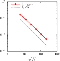
Fig. 4: Behavior of $(\frac{1}{2}-\sigma_{\max})$ versus total number of unknowns, $N$.

This is in agreement with (35).

6.2 Two subdomain case

In this section we compare the contraction factor of the two Schwarz algorithms with respect to $h$-dependency. We perform both algorithms on a sequence of unstructured meshes. We measure the number of iterations required to reduce the relative error to $tol:=1\mbox{\sc{e}-}10$ while refining the mesh, that is

$${\|u_{h}^{(n)}-u_{h}\|_{0}}\leq tol\,\|f\|_{0}.$$

This level of accuracy is not necessary in practice since the error between the exact and approximate solution, $\|u-u_{h}\|_{0}$, is much bigger and one usually can terminate the iteration after reaching the accuracy level of the method. The domain is partitioned into two by a non-straight interface; see Figure 1 (left).

As we see in the Figure 5 (left),

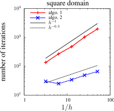
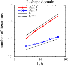
Fig. 5: Convergence of Schwarz methods on a square domain (left) and L-shape domain (right).

on a square domain the number of iterations for Algorithm 1 grows like $1/h$, which is equivalent to $\rho\leq 1-O(h)$, while for Algorithm 2 it behaves like $1/\sqrt{h}$, or in other words we have $\rho\leq 1-O(\sqrt{h})$, which illustrates well our analysis. This is the case for the L-shape domain too, see Figure 5 (right).

6.3 Multi subdomains case

We now show some numerical results on the multi subdomain algorithm. The subdomains are formed by a coarse triangulation of the domain which we call $\mathcal{T}_{H}$. We consider a nested fine mesh and therefore $\mathcal{T}_{H}\subset\mathcal{T}_{h}$. An example is given in Figure 1 (right). We consider here four subdomains which share a cross-point, and similarly to the two subdomain case we measure the number of iterations necessary to reach the desired tolerance. We observe in Table 2

Table 2: Convergence of OSM for four subdomains

Mesh size	$h_{0}$	$h_{0}/2$	$h_{0}/4$	$h_{0}/8$	$h_{0}/16$
# iterations	25	35	57	82	117

that the contraction factor asymptotically is $\rho=1-O(\sqrt{h})$, i.e. $82/57\approx 1.43$ or $117/82\approx 1.42$ which are close to $\sqrt{2}$.

6.4 OSM as a preconditioner

We use now the optimized Schwarz method as a preconditioner for GMRES with the tolerance $tol:=1\mbox{\sc{e}-}6$. In order to provide a qualitative comparison we also consider the widely used conjugate gradient method with a one-level additive Schwarz preconditioner applied to the original system (2). We consider 16 subdomains illustrated in Figure 1 (right). We observe in Table 3

Table 3: Number of iterations required by OSM-GMRES and PCG to reach the desired tolerance.

Mesh size	$h_{0}$	$h_{0}/2$	$h_{0}/4$	$h_{0}/8$	$h_{0}/16$
OSM-GMRES	20	52	60	72	87
PCG	14	38	55	104	154

that the number of iterations for OSM-GMRES grows like $O(h^{-1/4})$. This is because Krylov methods benefit often from another square-root in their contraction factor compared to the stationary iteration method. Therefore the contraction factor of OSM-GMRES is $\rho=1-O(h^{1/4})$, i.e. $72/60\approx 1.2,87/72\approx 1.2$ which are close to $2^{1/4}$. For preconditioned (additive Schwarz) conjugate gradient method, we have $\rho=1-O(\sqrt{h})$.

We would like to comment on the size of the augmented system. In case of mesh size $h_{0}/16$ we have 19,032 DOFs for the primal variable $u_{h}$ and 1,296 DOFs for the interface unknowns. Therefore the augmented system is very little changed in size compared to the original system.

7 Conclusion

We have presented and analyzed classical and optimized Schwarz methods for IPH discretizations. The interesting fact is that both use Robin transmission conditions, but we proved that for an arbitrary two-subdomain decomposition the classical Schwarz algorithm has a convergence factor $1-O(h)$, while the optimized one has a contraction factor $1-O(\sqrt{h})$. This is because the IPH discretization imposes a bad choice of the Robin parameter on the method. We then generalized the definition of the algorithms to the multi-subdomain case, and showed by numerical experiments that our theoretical results still hold. We finally illustrated the potential benefit that one obtains using OSM as a preconditioner compared to PCG.

proof of inequalities for ${\boldsymbol{\theta}}(\cdot)$

In this part we provide some proofs regarding the extension by zero operator, ${\boldsymbol{\theta}}_{i}(\cdot)$. First we recall inverse and mass matrix inequalities; see [25, Appendix B] and references therein. All constants are independent of $h$. Let $w\in\mathbb{P}^{1}(K)$ where $K$ is a simplex in $\mathbb{R}^{d}$. Then the inverse inequality

(51) $$\|\nabla w\|_{K}\leq\frac{c}{h}\|w\|_{K}$$

holds. Let ${\boldsymbol{w}}$ be the DOFs of $w$ and $M_{d}$ be the corresponding mass matrix. Then we have

$$c_{1}\,h^{d}\,{\boldsymbol{w}}^{\top}{\boldsymbol{w}}\leq{\boldsymbol{w}}^{\top}M_{d}{\boldsymbol{w}}\leq c_{2}\,h^{d}\,{\boldsymbol{w}}^{\top}{\boldsymbol{w}}.$$

Lemma 17.

Let $\varphi\in\Lambda_{h}$ and ${\boldsymbol{\theta}}_{i}(\varphi)$ be its extension by zero operator into $\Omega_{i}$. For an element $K$ which shares an edge with the interface, we have

$$\begin{array}[]{lcl}\|\nabla{\boldsymbol{\theta}}_{i}(\varphi)\|_{K}^{2}&\leq&{C_{1}}{h^{-1}}\|\varphi\|_{e}^{2},\\ \|{\boldsymbol{\theta}}_{i}(\varphi)\|_{K}^{2}&\leq&C_{2}\,h\|\varphi\|_{e}^{2}.\end{array}$$

Proof.

Let ${\boldsymbol{\varphi}}_{e}:=(\varphi_{1},\varphi_{2})$ be the DOFs of $\varphi$ on the edge shared with the interface. Moreover let $w={\boldsymbol{\theta}}_{i}(\varphi)|_{K}$. Then we have ${\boldsymbol{w}}=(\varphi_{1},\varphi_{2},0)$. For the first inequality we invoke the inverse inequality. Assuming the mesh is quasi-uniform, i.e. $h_{e}\approx h_{K}\approx h$, we get

$$\begin{array}[]{rcl}\|\nabla w\|_{K}^{2}\leq\frac{c^{2}}{h^{2}}\|w\|^{2}_{K}&\leq&c_{1}h^{d-2}(\varphi_{1}^{2}+\varphi_{2}^{2}+0)\\ &\leq&c_{2}h^{d-2}h_{e}^{-(d-1)}{\boldsymbol{\varphi}}_{e}^{\top}M_{d-1}{\boldsymbol{\varphi}}_{e}\\ &\leq&c_{3}h^{-1}{\boldsymbol{\varphi}}_{e}^{\top}M_{d-1}{\boldsymbol{\varphi}}_{e}\\ &=&c_{3}h^{-1}\|\varphi\|_{e}^{2}.\end{array}$$

The proof for the second inequality follows the same steps.  ∎

Lemma 18.

Let $\varphi\in\Lambda_{h}$ and ${\boldsymbol{\theta}}_{i}(\varphi)$ be its extension by zero operator into $\Omega_{i}$. Then

$$\|[\![{\boldsymbol{\theta}}_{i}(\varphi)]\!]\|_{\mathcal{E}_{i}}^{2}\leq C\|\varphi\|_{\Gamma}^{2},$$

where $C\geq 1$.

Proof.

We start by those edges which are part of the interface, see Figure 2, e.g. $e_{1}$ and $e_{3}$. We have

$$\sum_{e\in\Gamma}\|[\![{\boldsymbol{\theta}}_{i}(\varphi)]\!]\|_{e}^{2}=\sum_{e\in\Gamma}\|{\boldsymbol{\theta}}_{i}(\varphi)\|_{e}^{2}=\sum_{e\in\Gamma}\|\varphi\|_{e}^{2}=\|\varphi\|_{\Gamma}^{2},$$

which shows already that $C\geq 1$. Consider those edges $e\in\mathcal{E}_{i}$ that are not on the interface but belong to an element which shares an edge with the interface, e.g. $e^{\ast}:=\partial K_{1}\cap\partial K_{2}$ in Figure 2. Let ${\boldsymbol{\varphi}}_{e}:=(\varphi_{1},\varphi_{2})$ be the DOFs of $\varphi$ on $e_{2}$ and assume $\varphi_{2}$ is the DOF which is also located on $e^{\ast}$. Then we have

$$\|[\![{\boldsymbol{\theta}}_{i}(\varphi)]\!]\|^{2}_{e^{\ast}}=(\varphi_{2},0)M_{d-1}(\varphi_{2},0)^{\top}\leq ch_{e^{\ast}}^{d-1}\varphi_{2}^{2}\leq ch_{e^{\ast}}^{d-1}(\varphi_{2}^{2}+\varphi_{1}^{2})\leq c_{1}\|\varphi\|_{e}^{2},$$

where we again used the quasi-uniformity of the mesh ($h_{e}\approx h\approx h_{e^{\ast}}$). The other case would be $K_{1}$ and $K_{3}$ share an edge, for which we can use the same argument. For other edges $[\![{\boldsymbol{\theta}}_{i}(\varphi)]\!]$ is simply zero.  ∎

References

- [1] Paola F. Antonietti and Blanca Ayuso, Multiplicative schwarz methods for discontinuous galerkin approximations of elliptic problems, ESAIM: Mathematical Modelling and Numerical Analysis, 42 (2008), pp. 443–469.
- [2] Paola F Antonietti and Paul Houston, A class of domain decomposition preconditioners for hp-discontinuous galerkin finite element methods, Journal of Scientific Computing, 46 (2011), pp. 124–149.
- [3] Douglas N. Arnold, Franco Brezzi, Bernardo Cockburn, and L. Donatella Marini, Unified analysis of discontinuous Galerkin methods for elliptic problems, SIAM J. Numer. Anal., 39 (2001/02), pp. 1749–1779.
- [4] Susanne C. Brenner, The condition number of the Schur complement in domain decomposition, Numer. Math., 83 (1999), pp. 187–203.
- [5] , Poincaré-Friedrichs inequalities for piecewise functions, SIAM J. Numer. Anal., 41 (2003), pp. 306–324.
- [6] Paul Castillo, Performance of discontinuous Galerkin methods for elliptic PDEs, SIAM J. Sci. Comput., 24 (2002), pp. 524–547.
- [7] Bernardo Cockburn, Jayadeep Gopalakrishnan, and Raytcho Lazarov, Unified hybridization of discontinuous Galerkin, mixed, and continuous Galerkin methods for second order elliptic problems, SIAM J. Numer. Anal., 47 (2009), pp. 1319–1365.
- [8] Marco Discacciati, An operator-splitting approach to nonoverlapping domain decomposition methods, Rapport de la Section de Mathématiques, EPFL, (2004).
- [9] Maksymilian Dryja, Juan Galvis, and Marcus Sarkis, BDDC methods for discontinuous galerkin discretization of elliptic problems, Journal of Complexity, 23 (2007), pp. 715 – 739. Festschrift for the 60th Birthday of Henryk Woźniakowski.
- [10] Mohamed El Bouajaji, Victorita Dolean, Martin J Gander, Stephane Lanteri, Ronan Perrussel, et al., DG discretization of optimized Schwarz methods for Maxwell’s equations, (2013).
- [11] Richard E. Ewing, Junping Wang, and Yongjun Yang, A stabilized discontinuous finite element method for elliptic problems, Numer. Linear Algebra Appl., 10 (2003), pp. 83–104. Dedicated to the 60th birthday of Raytcho Lazarov.
- [12] Xiaobing Feng and Ohannes A. Karakashian, Two-level additive Schwarz methods for a discontinuous Galerkin approximation of second order elliptic problems, SIAM J. Numer. Anal., 39 (2001), pp. 1343–1365 (electronic).
- [13] Martin J. Gander, Optimized Schwarz methods, SIAM J. Numer. Anal., 44 (2006), pp. 699–731 (electronic).
- [14] Martin J Gander, Schwarz methods over the course of time, Electronic Transactions on Numerical Analysis, 31 (2008), p. 5.
- [15] Martin J. Gander and Soheil Hajian, Block Jacobi for discontinuous Galerkin discretizations: no ordinary Schwarz methods, Domain Decomposition Methods in Science and Engineering XXI, Lect. Notes Comput. Sci. Eng. Springer, (2013).
- [16] Martin J Gander and Felix Kwok, Best Robin parameters for optimized Schwarz methods at cross points, SIAM Journal on Scientific Computing, 34 (2012), pp. A1849–A1879.
- [17] , On the applicability of Lions’ energy estimates in the analysis of discrete optimized Schwarz methods with cross points, in Domain Decomposition Methods in Science and Engineering XX, Springer, 2013, pp. 475–483.
- [18] Martin J Gander and Kévin Santugini, Cross-points in domain decomposition methods with a finite element discretization, in preparation, (2014).
- [19] Claude J. Gittelson, Ralf Hiptmair, and Ilaria Perugia, Plane wave discontinuous galerkin methods: Analysis of the h-version, ESAIM: Mathematical Modelling and Numerical Analysis, 43 (2009), pp. 297–331.
- [20] Soheil Hajian, An optimized Schwarz algorithm for discontinuous Galerkin methods, Domain Decomposition Methods in Science and Engineering XXII, (2014).
- [21] Christoph Lehrenfeld, Hybrid discontinuous Galerkin methods for incompressible flow problems, master’s thesis, RWTH Aachen, 2010.
- [22] S. H. Lui, A Lions non-overlapping domain decomposition method for domains with an arbitrary interface, IMA J. Numer. Anal., 29 (2009), pp. 332–349.
- [23] Lizhen Qin and Xuejun Xu, On a parallel Robin-type nonoverlapping domain decomposition method, SIAM Journal on Numerical Analysis, 44 (2006), pp. pp. 2539–2558.
- [24] Joachim Schöberl and Christoph Lehrenfeld, Domain decomposition preconditioning for high order hybrid discontinuous galerkin methods on tetrahedral meshes, in Advanced Finite Element Methods and Applications, Thomas Apel and Olaf Steinbach, eds., vol. 66 of Lecture Notes in Applied and Computational Mechanics, Springer Berlin Heidelberg, 2013, pp. 27–56.
- [25] Andrea Toselli and Olof Widlund, Domain decomposition methods—algorithms and theory, vol. 34 of Springer Series in Computational Mathematics, Springer-Verlag, Berlin, 2005.
- [26] T. Warburton and J. S. Hesthaven, On the constants in -finite element trace inverse inequalities, Comput. Methods Appl. Mech. Engrg., 192 (2003), pp. 2765–2773.