Fractional differentiation matrices with applications

Abstract

In this paper, the fractional differential matrices based on the Jacobi-Gauss points are derived with respect to the Caputo and Riemann-Liouville fractional derivative operators. The spectral radii of the fractional differential matrices are investigated numerically. The spectral collocation schemes are illustrated to solve the fractional ordinary differential equations and fractional partial differential equations. Numerical examples are also presented to illustrate the effectiveness of the derived methods, which show better performances over some existing methods.

1 Introduction

Differential matrices are useful and easily implemented in the simulation of the classical differential equations [1, 32]. This paper aims to develop the fractional differential matrices to approximate the fractional integral and derivative operators with applications for solving the fractional differential equations.

Fractional calculus (including the fractional integral and the fractional derivative) has become a hot topic recently for its wide applications in many areas of science and engineering, see for example [7, 14, 21, 25, 26, 29, 31, 39, 42].

Unlike the classical derivative operator, the fractional derivative operators are nonlocal with weakly singularity, which are more complicated for theoretical analysis and numerical simulation. Up to now, there have been some numerical methods to discretize the fractional integral and derivative operators, for instance [2, 5, 6, 12, 13, 15, 16, 18, 20, 22, 23, 25, 24, 33, 34, 40, 41]. In [17, 35], the L1 method was proposed to discretize the Riemann-Liouville and Caputo derivative operators. Tian et al. [37] proposed the weighted formula based on the shifted Grünwald-Letnikov formula to approximate the Riemann–Liouville derivative operator with second-order accuracy. Çelik and Duman [3] proposed the fractional central difference method to discretize Riesz fractional derivative operator with convergence of order 2. The operational matrices based on the explicit forms of the Legendre, Chebyshev and Jacobi polynomials were proposed to discretize the Caputo derivative operator in [8, 9, 10, 11, 30]. Tian and Deng [36] proposed a method to approximate the Caputo fractional derivative operator with the fractional differential matrices obtained, but their method seems unstable when performing on the common computers with double precision. Xu and Hesthaven [38] also proposed the fractional differential matrix to approximate the Caputo derivative operator, but the derivation of the fractional differential matrix involves in calculating the inverse matrix. Recently, a multi-domain spectral method based on the multi-domain fractional differential matrix for time-fractional differential equation was developed in [4].

In [19], the effective recurrence formulas were developed to approximate the fractional integral and the left Caputo fractional derivative of the Legendre, Chebyshev, and Jacobi polynomials, and the corresponding operational matrices are obtained such that the fractional integral and derivative of a given function at one collocation point can be calculated with $O(N)$ operations. In this paper, we choose the collocation points as the Jacobi-Gauss types, such that the fractional differentiation of a given function $u(x),x\in[-1,1]$ at the collocation points $x_{j}\,(j=0,1,...,N)$ are approximated by the matrix-vector product, i.e., $A\mathbf{u}$, $A\in\mathbb{R}^{(N+1)\times(N+1)},\mathbf{u}=(u(x_{0}),u(x_{1}),...,u(x_{N}))^{T}$. We call such a type of matrix $A$ the fractional differential matrix. The spectral radius $\rho(A)$ of the fractional differential matrix $A$ is numerically investigated, which shows the behavior as $\rho(A){\,\leq\,}C_{0}N^{2\alpha}$, where $C_{0}$ is independent of $N$, $\alpha$ is the order of the corresponding fractional derivative operator. The spectral collocation schemes are illustrated to solve the fractional ordinary differential equations and the fractional partial differential equations. Numerical experiments display good satisfactory results, and the comparison between other methods are made to show better performances of the present methods.

The remainder of this paper is organized as follows. In Section 2, we introduce several definitions of fractional calculus and the Legendre, Chebyshev and Jacobi polynomials. The fractional differential matrices with respect to the Caputo and Riemann–Liouville derivative operators are derived in Section 3. The spectral collocation methods for solving the fractional differential equations are illustrated in Section 4. Numerical examples are presented in Section 5, and the conclusion is included in the last section.

2 Preliminaries

In this section, we introduce the definitions of the fractional calculus. Then we introduce the Legendre, Chebyshev and Jacobi polynomials, which will be used later on.

Definition 2.1

The left and right fractional integrals (or the left and right Riemann–Liouville integrals) with order $\alpha>0$ of the given function $f(t)$ are defined as

$$D^{-\alpha}_{a,t}f(t)=\frac{1}{\Gamma(\alpha)}\int_{a}^{t}(t-s)^{\alpha-1}f(s)\,{\rm d}s$$ (1)

and

$$D^{-\alpha}_{t,b}f(t)=\frac{1}{\Gamma(\alpha)}\int_{t}^{b}(s-t)^{\alpha-1}f(s)\,{\rm d}s$$ (2)

respectively, where $\Gamma(\cdot)$ is the Euler’s gamma function.

There exist several kinds of fractional derivatives, which will be introduced in the following.

Definition 2.2

The left and right Riemann-Liouville fractional derivatives with order $\alpha>0$ of the given function $f(t),t\,\in\,(a,b)$ are defined as

$${}_{C}D_{a,t}^{\alpha}f(t)=\frac{\mathrm{d}^{n}}{\mathrm{d}t^{n}}D^{-(n-\alpha)}_{a,t}f(t)=\frac{1}{\Gamma(n-\alpha)}\frac{\mathrm{d}^{n}}{\mathrm{d}t^{n}}\int_{a}^{t}(t-s)^{n-\alpha-1}f(s)\,{\rm d}s$$ (3)

and

$${}_{C}D_{t,a}^{\alpha}f(t)=(-1)^{n}\frac{\mathrm{d}^{n}}{\mathrm{d}t^{n}}D^{-(n-\alpha)}_{t,a}f(t)=\frac{(-1)^{n}}{\Gamma(n-\alpha)}\frac{\mathrm{d}^{n}}{\mathrm{d}t^{n}}\int_{t}^{b}(s-t)^{n-\alpha-1}f(s)\,{\rm d}s$$ (4)

respectively, where $n$ is a positive integer and $n-1<\alpha{\,\leq\,}n$.

Definition 2.3

The left and right Caputo fractional derivatives with order $\alpha>0$ of the given function $f(t),t\,\in\,(a,b)$ are defined as

$${}_{C}D_{a,t}^{\alpha}f(t)=D^{-(n-\alpha)}_{a,t}\Big{[}f^{(n)}(t)\Big{]}=\frac{1}{\Gamma(n-\alpha)}\int_{a}^{t}(t-s)^{n-\alpha-1}f^{(n)}(s)\,{\rm d}s$$ (5)

and

$${}_{C}D_{t,a}^{\alpha}f(t)=(-1)^{n}D^{-(n-\alpha)}_{t,a}\Big{[}f^{(n)}(t)\Big{]}=\frac{(-1)^{n}}{\Gamma(n-\alpha)}\int_{t}^{b}(s-t)^{n-\alpha-1}f^{(n)}(s)\,{\rm d}s$$ (6)

respectively, where $n$ is a positive integer and $n-1<\alpha{\,\leq\,}n$.

Definition 2.4

The Riesz fractional derivative and Riesz-Caputo fractional derivative with order $\alpha>0$ of the given function $f(t),t\,\in\,(a,b)$ are defined as

$${}_{RZ}D_{t}^{\alpha}f(t)=c_{\alpha}\Big{(}{}_{RL}D_{a,t}^{\alpha}f(t)+{}_{RL}D_{t,b}^{\alpha}f(t)\Big{)},$$ (7)

and

$${}_{RC}D_{t}^{\alpha}f(t)=c_{\alpha}\Big{(}{}_{C}D_{a,t}^{\alpha}f(t)+{}_{C}D_{t,b}^{\alpha}f(t)\Big{)},$$ (8)

respectively, where $c_{\alpha}=-\frac{1}{2\cos(\frac{\pi\alpha}{2})}$.

Next, we introduce the Jacobi polynomials. The Jacobi polynomials $\{P^{a,b}_{j}(x)\},\,a,b>-1,x\in[-1,1]$ are given by the following three-term recurrence relation [32]

$$P^{a,b}_{0}(x)=1,{\quad}P^{a,b}_{1}(x)=\frac{1}{2}(a+b+2)x+\frac{1}{2}(a-b),$$ (9)

$$P^{a,b}_{j+1}(x)=(A_{j}^{a,b}x-B_{j}^{a,b})P^{a,b}_{j}(x)-C_{j}^{a,b}P^{a,b}_{j-1}(x),\quad{n\geq 1},$$

where

$$A_{j}^{a,b}=\frac{(2j+a+b+1)(2j+a+b+2)}{2(j+1)(j+a+b+1)},$$ (10)

$$B_{j}^{a,b}=\frac{(b^{2}-a^{2})(2j+a+b+1)}{2(j+1)(j+a+b+1)(2j+a+b)},$$

$$C_{j}^{a,b}=\frac{(j+a)(j+b)(2j+a+b+2)}{(j+1)(j+a+b+1)(2j+a+b)}.$$

Next, several properties of the Jacobi polynomials will be stated. Let $\omega^{a,b}(x)=(1-x)^{a}(1+x)^{b}.$ Then, one has

$$\int_{-1}^{1}P^{a,b}_{m}(x)P^{a,b}_{n}(x)\omega^{a,b}(x)\,{\rm d}x=\left\{\begin{aligned} &0,{\quad}m\neq n\\ &\gamma^{a,b}_{n},{\quad}m=n,\end{aligned}\right.$$ (11)

where

$$\gamma^{a,b}_{n}=\frac{2^{a+b+1}\Gamma(n+a+1)\Gamma(n+b+1)}{(2n+a+b+1)n!\Gamma(n+a+b+1)}.$$ (12)

Some other properties of the Jacobi polynomials that will be used in the present paper are presented below:

$$P^{a,b}_{j}(1)=\binom{j+a}{j}=\frac{\Gamma(j+a+1)}{j!\Gamma(a+1)},{\quad}P^{a,b}_{j}(-1)=(-1)^{j}\frac{\Gamma(j+b+1)}{j!\Gamma(b+1)}.$$ (13)

$$\frac{{\rm d}^{m}}{\,{\rm d}x^{m}}P^{a,b}_{j}(x)=d_{j,m}^{a,b}P^{a+m,b+m}_{j-m}(x),\quad j{\,\geq\,}m,m\in\mathbb{N},$$ (14)

where

$$d_{j,m}^{a,b}=\frac{\Gamma(j+m+a+b+1)}{2^{m}\Gamma(j+a+b+2)}.$$ (15)

$$P^{a,b}_{j}(x)=\widehat{A}_{j}^{a,b}\frac{{\rm d}}{\,{\rm d}x}P^{a,b}_{j-1}(x)+\widehat{B}_{j}^{a,b}\frac{{\rm d}}{\,{\rm d}x}P^{a,b}_{j}(x)+\widehat{C}_{j}^{a,b}\frac{{\rm d}}{\,{\rm d}x}P^{a,b}_{j+1}(x),\quad{j\geq 1},$$ (16)

in which

$$\widehat{A}_{j}^{a,b}=\frac{-2(j+a)(j+b)}{(j+a+b)(2j+a+b)(2j+a+b+1)},$$ (17)

$$\widehat{B}_{j}^{a,b}=\frac{2(a-b)}{(2j+a+b)(2j+a+b+2)},$$

$$\widehat{C}_{j}^{a,b}=\frac{2(j+a+b+1)}{(2j+a+b+1)(2j+a+b+2)}.$$

If $j=1$, then $\widehat{A}_{1}^{a,b}=0$ in (17).

If $a=b=0$, then the recurrence formula (9) is reduced to the Legendre polynomials as

$$L_{0}(x)=1,{\quad}L_{1}(x)=x,{\quad}L_{j+1}=\frac{2j+1}{j+1}xL_{j}(x)-\frac{j}{j+1}L_{j-1}(x),\quad{j\geq 1}.$$ (18)

If $a=b=-1/2$ in (9), then $P^{-\frac{1}{2},-\frac{1}{2}}_{j}(x)=\frac{\Gamma(j+1/2)}{j!\sqrt{\pi}}T_{j}(x)$, where $T_{j}(x)$ is the Chebyshev polynomial that can be defined as

$$T_{0}(x)=1,{\quad}T_{1}(x)=x,{\quad}T_{j+1}(x)=2xT_{j}(x)-T_{j-1}(x),\quad{j\geq 1}.$$ (19)

3 Derivations of the fractional differential matrices

Denote by

$$\widehat{P}_{L,j}^{a,b,\alpha}(x)=\frac{1}{\Gamma(\alpha)}\int_{-1}^{x}(x-s)^{\alpha-1}P^{a,b}_{j}(s)\,{\rm d}s.$$

Using the recurrence formulae (9)–(10), the properties (13) and (16), we have

$$\left\{\begin{aligned} &\widehat{P}_{L,0}^{a,b,\alpha}(x)=\frac{(x+1)^{\alpha}}{\Gamma(\alpha+1)},\\ &\widehat{P}_{L,1}^{a,b,\alpha}(x)=\frac{a+b+2}{2}\left(\frac{x(x+1)^{\alpha}}{\Gamma(\alpha+1)}-\frac{\alpha(x+1)^{\alpha+1}}{\Gamma(\alpha+2)}\right)+\frac{a-b}{2}\widehat{P}_{L,0}^{a,b,\alpha}(x),\\ &\widehat{P}_{L,j+1}^{a,b,\alpha}(x)=\frac{A_{j}^{a,b}x-B_{j}^{a,b}-{\alpha}A_{j}^{a,b}\widehat{B}_{j}^{a,b}}{1+{\alpha}A_{j}^{a,b}\widehat{C}_{j}^{a,b}}\widehat{P}_{L,j}^{a,b,\alpha}(x)-\frac{C_{j}^{a,b}+{\alpha}A_{j}^{a,b}\widehat{A}_{j}^{a,b}}{1+{\alpha}A_{j}^{a,b}\widehat{C}_{j}^{a,b}}\widehat{P}_{L,j-1}^{a,b,\alpha}(x)\\ &{\quad}+\frac{{\alpha}A_{j}^{a,b}\left(\widehat{A}_{j}^{a,b}P^{a,b}_{j-1}(-1)+\widehat{B}_{j}^{a,b}P^{a,b}_{j}(-1)+\widehat{C}_{j}^{a,b}P^{a,b}_{j+1}(-1)\right)}{\Gamma(\alpha+1)\left(1+{\alpha}A_{j}^{a,b}\widehat{C}_{j}^{a,b}\right)}(x+1)^{\alpha},{\quad\quad}j{\,\geq\,}1.\end{aligned}\right.$$ (20)

The above recurrence formula was first obtained in [19]. Denote by

$$\widehat{P}_{R,j}^{a,b,\alpha}(x)=\frac{1}{\Gamma(\alpha)}\int_{x}^{1}(s-x)^{\alpha-1}P^{a,b}_{j}(s)\,{\rm d}s.$$

For $j{\,\geq\,}1$, we can obtain from (9) that

$$\widehat{P}_{R,j+1}^{a,b,\alpha}(x)= \frac{1}{\Gamma(\alpha)}\int_{x}^{1}(s-x)^{\alpha-1}P^{a,b}_{j+1}(s)\,{\rm d}s$$ (21)

$$= \frac{1}{\Gamma(\alpha)}\int_{x}^{1}(s-x)^{\alpha-1}\left[(A_{j}^{a,b}s-B_{j}^{a,b})P^{a,b}_{j}(s)-C_{j}^{a,b}P^{a,b}_{j-1}(s)\right]\,{\rm d}s$$

$$= (A_{j}^{a,b}x-B_{j}^{a,b})\widehat{P}_{R,j}^{a,b,\alpha}(x)-C_{j}^{a,b}\widehat{P}_{R,j-1}^{a,b,\alpha}(x)+\frac{A_{j}^{a,b}}{\Gamma(\alpha)}\int_{x}^{1}(s-x)^{\alpha}P^{a,b}_{j}(s)\,{\rm d}s.$$

Using (16) yields

$$\widehat{P}_{R,j+1}^{a,b,\alpha}(x)= (A_{j}^{a,b}x-B_{j}^{a,b})\widehat{P}_{R,j}^{a,b,\alpha}(x)-C_{j}^{a,b}\widehat{P}_{R,j-1}^{a,b,\alpha}(x)$$ (22)

$$+\frac{A_{j}^{a,b}}{\Gamma(\alpha)}\int_{x}^{1}(s-x)^{\alpha}\,\mathrm{d}\left[\widehat{A}_{j}^{a,b}P^{a,b}_{j-1}(s)+\widehat{B}_{j}^{a,b}P^{a,b}_{j}(s)+\widehat{C}_{j}^{a,b}P^{a,b}_{j+1}(s)\right]$$

$$= (A_{j}^{a,b}x-B_{j}^{a,b})\widehat{P}_{R,j}^{a,b,\alpha}(x)-C_{j}^{a,b}\widehat{P}_{R,j-1}^{a,b,\alpha}(x)$$

$$+\frac{A_{j}^{a,b}}{\Gamma(\alpha)}(s-x)^{\alpha}\left[\widehat{A}_{j}^{a,b}P^{a,b}_{j-1}(s)+\widehat{B}_{j}^{a,b}P^{a,b}_{j}(s)+\widehat{C}_{j}^{a,b}P^{a,b}_{j+1}(s)\right]\bigg{|}_{x}^{1}$$

$$-\frac{{\alpha}A_{j}^{a,b}}{\Gamma(\alpha)}\int_{x}^{1}(s-x)^{\alpha-1}\left[\widehat{A}_{j}^{a,b}P^{a,b}_{j-1}(s)+\widehat{B}_{j}^{a,b}P^{a,b}_{j}(s)+\widehat{C}_{j}^{a,b}P^{a,b}_{j+1}(s)\right]\,{\rm d}s$$

$$= (A_{j}^{a,b}x-B_{j}^{a,b})\widehat{P}_{R,j}^{a,b,\alpha}(x)-C_{j}^{a,b}\widehat{P}_{R,j-1}^{a,b,\alpha}(x)$$

$$-{\alpha}A_{j}^{a,b}\left(\widehat{A}_{j}^{a,b}\widehat{P}^{a,b}_{R,j-1}(s)+\widehat{B}_{j}^{a,b}\widehat{P}^{a,b}_{R,j}(s)+\widehat{C}_{j}^{a,b}\widehat{P}^{a,b}_{R,j+1}(s)\right)$$

$$+\frac{A_{j}^{a,b}}{\Gamma(\alpha)}(1-x)^{\alpha}\left[\widehat{A}_{j}^{a,b}P^{a,b}_{j-1}(1)+\widehat{B}_{j}^{a,b}P^{a,b}_{j}(1)+\widehat{C}_{j}^{a,b}P^{a,b}_{j+1}(1)\right].$$

Note that $\widehat{P}_{R,0}^{a,b,\alpha}(x)$ and $\widehat{P}_{R,1}^{a,b,\alpha}(x)$ can be easily calculated. Hence, we derive the recurrence relation from (22) below

$$\left\{\begin{aligned} &\widehat{P}_{R,0}^{a,b,\alpha}(x)=\frac{(1-x)^{\alpha}}{\Gamma(\alpha+1)},\\ &\widehat{P}_{R,1}^{a,b,\alpha}(x)=\frac{a+b+2}{2}\left(\frac{x(1-x)^{\alpha}}{\Gamma(\alpha+1)}+\frac{\alpha(1-x)^{\alpha+1}}{\Gamma(\alpha+2)}\right)+\frac{a-b}{2}\widehat{P}_{R,0}^{a,b,\alpha}(x),\\ &\widehat{P}_{R,j+1}^{a,b,\alpha}(x)=\frac{A_{j}^{a,b}x-(B_{j}^{a,b}+{\alpha}A_{j}^{a,b}\widehat{B}_{j}^{a,b})}{1+{\alpha}A_{j}^{a,b}\widehat{C}_{j}^{a,b}}\widehat{P}_{R,j}^{a,b,\alpha}(x)-\frac{C_{j}^{a,b}+{\alpha}A_{j}^{a,b}\widehat{A}_{j}^{a,b}}{1+{\alpha}A_{j}^{a,b}\widehat{C}_{j}^{a,b}}\widehat{P}_{R,j-1}^{a,b,\alpha}(x)\\ &{\quad}+\frac{{\alpha}A_{j}^{a,b}\left(\widehat{A}_{j}^{a,b}P^{a,b}_{j-1}(1)+\widehat{B}_{j}^{a,b}P^{a,b}_{j}(1)+\widehat{C}_{j}^{a,b}P^{a,b}_{j+1}(1)\right)}{\Gamma(\alpha+1)\left(1+{\alpha}A_{j}^{a,b}\widehat{C}_{j}^{a,b}\right)}(1-x)^{\alpha},{\quad\quad}j{\,\geq\,}1.\end{aligned}\right.$$ (23)

If $a=b=0$, the recurrence formulas (20) and (23) are reduced to

$$\left\{\begin{aligned} \widehat{L}_{L,0}^{\alpha}(x)&=\frac{(x+1)^{\alpha}}{\Gamma(\alpha+1)},\quad\widehat{L}_{L,1}^{\alpha}(x)=\frac{x(x+1)^{\alpha}}{\Gamma(\alpha+1)}-\frac{\alpha(x+1)^{\alpha+1}}{\Gamma(\alpha+2)},\\ \widehat{L}_{L,j+1}^{\alpha}(x)&=\frac{1}{j+1+\alpha}\Big{\{}(2j+1)x\widehat{L}_{L,j}^{\alpha}(x)-(j-\alpha)\widehat{L}_{L,j-1}^{\alpha}(x)\Big{\}},{\quad}j{\,\geq\,}1\end{aligned}\right.$$ (24)

and

$$\left\{\begin{aligned} \widehat{L}_{R,0}^{\alpha}(x)&=\frac{(1-x)^{\alpha}}{\Gamma(\alpha+1)},\quad\widehat{L}_{R,1}^{\alpha}(x)=\frac{x(1-x)^{\alpha}}{\Gamma(\alpha+1)}+\frac{\alpha(1-x)^{\alpha+1}}{\Gamma(\alpha+2)},\\ \widehat{L}_{R,j+1}^{\alpha}(x)&=\frac{1}{j+1+\alpha}\Big{\{}(2j+1)x\widehat{L}_{R,j}^{\alpha}(x)-(j-\alpha)\widehat{L}_{R,j-1}^{\alpha}(x)\Big{\}},{\quad}j{\,\geq\,}1,\end{aligned}\right.$$ (25)

respectively, where $\widehat{L}_{L,j}^{\alpha}(x)=\widehat{P}_{L,j}^{0,0,\alpha}(x)$ and $\widehat{L}_{R,j}^{\alpha}(x)=\widehat{P}_{R,j}^{0,0,\alpha}(x)$.

For $a=b=-1/2$, from (20), (23), and the relation $P^{-\frac{1}{2},-\frac{1}{2}}_{j}(x)=\frac{\Gamma(j+1/2)}{j!\sqrt{\pi}}T_{j}(x)$, one can obtain

$$\left\{\begin{aligned} \widehat{T}_{L,0}^{\alpha}(x)=&\frac{(x+1)^{\alpha}}{\Gamma(\alpha+1)},{\qquad}\widehat{T}_{L,1}^{\alpha}(x)=\frac{x(x+1)^{\alpha}}{\Gamma(\alpha+1)}-\frac{\alpha(x+1)^{\alpha+1}}{\Gamma(\alpha+2)},\\ \widehat{T}_{L,2}^{\alpha}(x)=&\frac{2(1+x)^{2+\alpha}}{\Gamma(3+\alpha)}-\frac{4(1+x)^{1+\alpha}}{\Gamma(2+\alpha)}+\frac{(1+x)^{\alpha}}{\Gamma(1+\alpha)},\\ \widehat{T}_{L,j+1}^{\alpha}(x)=&\frac{2(j+1)x}{j+1+\alpha}\widehat{T}_{L,j}^{\alpha}(x)-\frac{(j+1)(j-1-\alpha)}{(j+1+\alpha)(j-1)}\widehat{T}_{L,j-1}^{\alpha}(x)\\ &+\frac{2(-1)^{j}\alpha(x+1)^{\alpha}}{\Gamma(\alpha+1)(j+1+\alpha)(j-1)},\quad j{\,\geq\,}2\end{aligned}\right.$$ (26)

and

$$\left\{\begin{aligned} \widehat{T}_{R,0}^{\alpha}(x)=&\frac{(1-x)^{\alpha}}{\Gamma(\alpha+1)},{\qquad}\widehat{T}_{R,1}^{\alpha}(x)=\frac{x(1-x)^{\alpha}}{\Gamma(\alpha+1)}+\frac{\alpha(1-x)^{\alpha+1}}{\Gamma(\alpha+2)},\\ \widehat{T}_{R,2}^{\alpha}(x)=&\frac{2(1-x)^{2+\alpha}}{\Gamma(3+\alpha)}-\frac{4(1-x)^{1+\alpha}}{\Gamma(2+\alpha)}+\frac{(1-x)^{\alpha}}{\Gamma(1+\alpha)},\\ \widehat{T}_{R,j+1}^{\alpha}(x)=&\frac{2(j+1)x}{j+1+\alpha}\widehat{T}_{R,j}^{\alpha}(x)-\frac{(j+1)(j-1-\alpha)}{(j+1+\alpha)(j-1)}\widehat{T}_{R,j-1}^{\alpha}(x)\\ &+\frac{2\alpha(1-x)^{\alpha}}{\Gamma(\alpha+1)(j+1+\alpha)(j-1)},\quad j{\,\geq\,}2,\end{aligned}\right.$$ (27)

respectively, where $\widehat{T}_{L,j}^{\alpha}(x)=\frac{1}{\Gamma(\alpha)}\int_{-1}^{x}(x-s)^{\alpha-1}T_{j}(s)\,{\rm d}s$ and $\widehat{T}_{R,j}^{\alpha}(x)=\frac{1}{\Gamma(\alpha)}\int_{x}^{1}(s-x)^{\alpha-1}T_{j}(s)\,{\rm d}s$. One can refer to [19], in which the detailed derivations of (24) and (26) can be found.

Let $u(x)$ be a function defined on the interval $[-1,1]$ and $N$ be a positive integer. Denote $x_{j}(j=0,1,...,N)$ as the Jacobi–Gauss–Lobatto (JGL) points defined on the interval $[-1,1]$. Then the JGL interpolation of $u(x)$ is given by

$$I_{N}u(x)=\sum_{j=0}^{N}u(x_{j})F_{j}(x)=\sum_{j=0}^{N}\tilde{p}_{j}P_{j}^{a,b}(x),$$ (28)

where $F_{j}(x)$ is the Lagrange base function.

In [19], authors obtained the formulas for numerically calculating $D_{-1,x}^{-\alpha}I_{N}u(x)$ and ${}_{C}D^{\alpha}_{-1,x}I_{N}u(x)$ on the JGL points $\{x_{j}\}$. $D_{-1,x}^{-\alpha}I_{N}u(x)(\alpha>0)$ at $x=x_{j},j=0,1,...,N$ can be calculated by the following formula [19]

$$\left(\begin{array}[]{c}D_{-1,x_{0}}^{-\alpha}I_{N}u(x_{0})\\ D_{-1,x_{1}}^{-\alpha}I_{N}u(x_{1})\\ \vdots\\ D_{-1,x_{N}}^{-\alpha}I_{N}u(x_{N})\end{array}\right)={\widehat{D}}^{(a,b,\alpha)}_{L}(\tilde{p}_{0},\tilde{p}_{1},\cdots,\tilde{p}_{N})^{T},$$ (29)

where $D_{-1,x_{i}}^{-\alpha}I_{N}u(x_{i})=\left[D_{-1,x}^{-\alpha}I_{N}u\right]_{x=x_{i}}$ and ${\widehat{D}}^{(a,b,\alpha)}_{L}\in\mathbb{R}^{(N+1)\times(N+1)}$ satisfying

$$\left({\widehat{D}}^{(a,b,\alpha)}_{L}\right)_{i,j}=\widehat{P}_{L,j}^{a,b,\alpha}({x}_{i}),{\quad}i,j=0,...,N.$$

The computation of ${}_{C}{D}^{\alpha}_{-1,x}I_{N}u(x)(n-1<\alpha<n,n\in Z^{+})$ at $x=x_{j},j=0,1,...,N$ is given by [19]

$$\left(\begin{array}[]{c}D_{-1,x_{0}}^{\alpha}I_{N}u(x_{0})\\ D_{-1,x_{1}}^{\alpha}I_{N}u(x_{1})\\ \vdots\\ D_{-1,x_{N}}^{\alpha}I_{N}u(x_{N})\end{array}\right)={}_{C}{\widehat{D}}_{L}^{(a,b,\alpha)}(\tilde{p}_{0},\tilde{p}_{1},\cdots,\tilde{p}_{N})^{T},$$ (30)

where ${}_{C}D_{-1,x_{i}}^{\alpha}I_{N}u(x_{i})=\left[{}_{C}D_{-1,x}^{\alpha}I_{N}u\right]_{x=x_{i}}$ and ${}_{C}{\widehat{D}}^{(a,b,\alpha)}_{L}\in\mathbb{R}^{(N+1)\times(N+1)}$ satisfying

$$\left({}_{C}{\widehat{D}}_{L}^{(a,b,\alpha)}\right)_{i,j}=d_{j,n}^{a,b}\,\widehat{P}^{a+n,b+n,n-\alpha}_{L,j}(x_{i}),{\quad}i,j=0,...,N$$

with $d_{j,n}^{a,b}$ given by (15).

Suppose that the Lagrange base function $F_{j}(x)$ can be expressed as

$$F_{j}(x)=\sum_{k=0}^{N}c_{k,j}P_{k}^{a,b}(x).$$ (31)

Then $c_{k,j}$ can be determined by the following relation [32]

$$c_{k,j}=\left\{\begin{aligned} &\frac{P_{k}^{a,b}(x_{j})\omega_{j}}{\gamma_{k}^{a,b}},{\,\,\,\,\qquad}k=0,1,...,N-1,\\ &\frac{P_{N}^{a,b}(x_{j})\omega_{j}}{(2+\frac{a+b+1}{N})\gamma_{N}^{a,b}},{\quad}k=N,\end{aligned}\right.$$ (32)

in which $\gamma_{k}^{a,b}$ is defined by (12), $x_{j}$ is the JGL point on $[-1,1]$.

From (28), (31), and (32), we obtain

$$\left(\begin{array}[]{c}\tilde{p}_{0}^{a,b}\\ \tilde{p}_{1}^{a,b}\\ \vdots\\ \tilde{p}_{N}^{a,b}\\ \end{array}\right)=\left(\begin{array}[]{cccc}c_{0,0}&c_{0,1}&\cdots&c_{0,N}\\ c_{1,0}&c_{1,1}&\cdots&c_{1,N}\\ \vdots&\vdots&\ddots&\vdots\\ c_{N,0}&c_{N,1}&\cdots&c_{N,N}\\ \end{array}\right)\left(\begin{array}[]{c}u(x_{0})\\ u(x_{1})\\ \vdots\\ u(x_{N})\\ \end{array}\right)=M(u(x_{0}),u(x_{1}),\cdots,u(x_{N}))^{T}.$$ (33)

Hence, the fractional integral $D_{-1,x}^{-\alpha}I_{N}u(x)$ at $x=x_{j}$ defined by (29) can be written into the following equivalent form

$$\left(\begin{array}[]{c}D_{-1,x_{0}}^{-\alpha}I_{N}u(x_{0})\\ D_{-1,x_{1}}^{-\alpha}I_{N}u(x_{1})\\ \vdots\\ D_{-1,x_{N}}^{-\alpha}I_{N}u(x_{N})\end{array}\right)=\left({\widehat{D}}^{(a,b,\alpha)}_{L}M\right)(u(x_{0}),u(x_{1}),\cdots,u(x_{N}))^{T},$$ (34)

where the matrices ${D}^{(a,b,\alpha)}_{L}$ and $M$ are defined as in (29) and (33), respectively. We can similarly obtain the equivalent form of (30) as follows

$$\left(\begin{array}[]{c}{}_{C}D_{-1,x_{0}}^{\alpha}I_{N}u(x_{0})\\ {}_{C}D_{-1,x_{1}}^{\alpha}I_{N}u(x_{1})\\ \vdots\\ {}_{C}D_{-1,x_{N}}^{\alpha}I_{N}u(x_{N})\end{array}\right)=\left({}_{C}{\widehat{D}}^{(a,b,\alpha)}_{L}M\right)(u(x_{0}),u(x_{1}),\cdots,u(x_{N}))^{T},$$ (35)

where the matrices ${}_{C}{D}^{(a,b,\alpha)}_{L}$ and $M$ are defined as in (30) and (33), respectively.

Next, we define the matrix ${}_{C}{D}^{(a,b,\alpha)}_{L},\alpha\in\mathbb{R}$ as follows:

$${}_{C}{D}^{(a,b,\alpha)}_{L}=\left\{\begin{aligned} &{\widehat{D}}^{(a,b,-\alpha)}_{L}M,{\quad}{\quad}M\text{ and }{\widehat{D}}^{(a,b,-\alpha)}_{L}\text{ are defined as in \eqref{eq:fint11} for }\alpha<0,\\ &{}_{C}{\widehat{D}}^{(a,b,\alpha)}_{L}M,{\quad}{\quad}M\text{ and }{}_{C}{\widehat{D}}^{(a,b,\alpha)}_{L}\text{ are defined as in \eqref{eq:fint12} for }\alpha>0.\end{aligned}\right.$$ (36)

We call the matrix ${}_{C}D_{L}^{(a,b,\alpha)}(\alpha>0)$ the fractional differential matrix with respect to the left Caputo derivative operator. We can similarly obtain the corresponding fractional differential matrix ${}_{C}D_{R}^{(a,b,\alpha)}$ with respect to the right fractional integral and Caputo derivative operators.

Since the left Caputo and Riemann–Liouville derivative operators have the following relation

$${}_{RL}D_{x_{0},x}^{\alpha}f(x)={}_{C}D_{x_{0},x}^{\alpha}f(x)+\sum_{k=0}^{n-1}\frac{f^{(k)}(x_{0})(x-x_{0})^{k-\alpha}}{\Gamma(k+1-\alpha)},{\quad}n-1<\alpha<n,n\in\mathbb{N}.$$ (37)

Hence, we can obtain

$$\left(\begin{array}[]{c}{}_{RL}D_{-1,x_{0}}^{\alpha}I_{N}u(x_{0})\\ {}_{RL}D_{-1,x_{1}}^{\alpha}I_{N}u(x_{1})\\ \vdots\\ {}_{RL}D_{-1,x_{N}}^{\alpha}I_{N}u(x_{N})\end{array}\right)=\left({}_{RL}{{D}}^{(a,b,\alpha)}_{L}\right)(u(x_{0}),u(x_{1}),\cdots,u(x_{N}))^{T},$$ (38)

where ${}_{RL}D_{-1,x_{i}}^{\alpha}I_{N}u(x_{i})=\left[{}_{RL}D_{-1,x}^{\alpha}I_{N}u\right]_{x=x_{i}}$ and the matrix ${}_{RL}{{D}}^{(a,b,\alpha)}_{L}\in\mathbb{R}^{(N+1)\times(N+1)}$ satisfying

$$\left({}_{RL}{{D}}^{(a,b,\alpha)}_{L}\right)_{i,j}=\left({}_{C}{{D}}^{(a,b,\alpha)}_{L}\right)_{i,j}+\sum_{k=0}^{n-1}\frac{D^{(k)}_{0,j}(x_{i}+1)^{k-\alpha}}{\Gamma(k+1-\alpha)},{\quad}i,j=0,1,\cdots,N,$$ (39)

in which ${}_{RL}D_{-1,x_{i}}^{\alpha}I_{N}u(x_{i})=\left[{}_{RL}D_{-1,x}^{\alpha}I_{N}u\right]_{x=x_{i}}$ and $D^{(k)}={}_{C}{D}^{(a,b,k)}_{L}$ is the $k$th-order classical differential matrix, see [32] for more information. We can similarly obtain

$$\left(\begin{array}[]{c}{}_{RL}D_{x_{0},1}^{\alpha}I_{N}u(x_{0})\\ {}_{RL}D_{x_{1},1}^{\alpha}I_{N}u(x_{1})\\ \vdots\\ {}_{RL}D_{x_{N},1}^{\alpha}I_{N}u(x_{N})\end{array}\right)=\left({}_{RL}{{D}}^{(a,b,\alpha)}_{R}\right)(u(x_{0}),u(x_{1}),\cdots,u(x_{N}))^{T},$$ (40)

where ${}_{RL}D_{x_{i},1}^{\alpha}I_{N}u(x_{i})=\left[{}_{RL}D_{x,1}^{\alpha}I_{N}u\right]_{x=x_{i}}$ and the matrix ${}_{RL}{{D}}^{(a,b,\alpha)}_{R}\in\mathbb{R}^{(N+1)\times(N+1)}$ satisfying

$$\left({}_{RL}{{D}}^{(a,b,\alpha)}_{R}\right)_{i,j}=\left({}_{C}{{D}}^{(a,b,\alpha)}_{R}\right)_{i,j}+\sum_{k=0}^{n-1}\frac{(-1)^{k}D^{(k)}_{N,j}(1-x_{i})^{k-\alpha}}{\Gamma(k+1-\alpha)},{\quad}i,j=0,1,\cdots,N.$$ (41)

Remark 3.1

Note that the first row of the matrix ${}_{RL}{{D}}^{(a,b,\alpha)}_{L}$ and the last row of the matrix ${}_{RL}{{D}}^{(a,b,\alpha)}_{R}$ have no sense, except that $\alpha$ is a positive integer, i.e., $\alpha=n,n\in\mathbb{N}$, and we set ${}_{RL}{{D}}^{(a,b,n)}_{L}={}_{C}{{D}}^{(a,b,n)}_{L}$ and ${}_{RL}{{D}}^{(a,b,n)}_{R}={}_{C}{{D}}^{(a,b,n)}_{R}$.

Next, we investigate the eigenvalues of the fractional differential operators. Consider first the following model problem

$$D^{\alpha}u(x)=\lambda u(x),x\in(-1,1),{\quad}u(-1)=u(1)=0,{\quad}1<\alpha{\,\leq\,}2.$$ (42)

where $D^{\alpha}$ denotes the left (or right) Caputo derivative operator ${}_{C}D_{-1,x}^{\alpha}$ (or ${}_{C}D_{x,1}^{\alpha}$), the left (or right) Riemann–Liouville derivative operator ${}_{RL}D_{-1,x}^{\alpha}$ (or ${}_{RL}D_{x,1}^{\alpha}$), the Riesz-Caputo fractional derivative operator ${}^{C}_{RZ}D_{x}^{\alpha}$, or the Riesz fractional derivative operator ${}_{RZ}D_{x}^{\alpha}$.

For simplicity, we first consider the case $D^{\alpha}={}_{C}D_{-1,x}^{\alpha}$ in (42). Denote ${x}_{i}(i=0,1,...,N)$ as the JGL points on the interval $[-1,1]$. Suppose that $u(x)$ can be approximated by

$$u(x)\approx I_{N}u(x)=\sum_{j=0}^{N}u_{j}F_{j}(x).$$ (43)

Replacing $u(x)$ with $I_{N}u(x)$ in (42) and letting $x={x}_{i}$ yield

$$\left[{}_{C}D_{-1,x}^{\alpha}I_{N}u(x)\right]_{x={x}_{i}}=\lambda(I_{N}u)({x}_{i}),{\quad}i=1,2,...,N-1.$$ (44)

Using the boundary conditions $(I_{N}u)(-1)=(I_{N}u)(1)=0$, we obtain the matrix representation of (44) as follows

$$M_{C,L}^{(\alpha,a,b)}\mathbf{u}=\lambda\mathbf{u},$$ (45)

where $\mathbf{u}=(u_{1},u_{2},...,u_{N-1})^{T}$ and $M_{C,L}^{(\alpha,a,b)}\in\mathbb{R}^{(N-1)\times(N-1)}$ satisfying

$$\left(M_{C,L}^{(\alpha,a,b)}\right)_{i,j}=\left({}_{C}{{D}}^{(a,b,\alpha)}_{L}\right)_{i+1,j+1},{\quad}i,j=0,1,...,N-2.$$

If $D^{\alpha}$ in (42) is chosen as $D^{\alpha}={}_{C}D_{x,1}^{\alpha}$, $D^{\alpha}={}_{RL}D_{-1,x}^{\alpha}$, $D^{\alpha}={}_{RL}D_{x,1}^{\alpha}$, $D^{\alpha}={}^{C}_{RZ}D_{x}^{\alpha}$, or $D^{\alpha}={}_{RZ}D_{x}^{\alpha}$, then we can similarly derive the linear system as (45) with the coefficient matrices denoted by $M_{C,R}^{(\alpha,a,b)}$, $M_{RL,L}^{(\alpha,a,b)}$, $M_{RL,R}^{(\alpha,a,b)}$, $M_{C,RZ}^{(\alpha,a,b)}$, or $M_{RZ}^{(\alpha,a,b)}$. Denote by $M_{1}^{(\alpha,a,b)}=M_{C,L}^{(\alpha,a,b)}$, $M_{2}^{(\alpha,a,b)}=M_{C,R}^{(\alpha,a,b)}$, $M_{3}^{(\alpha,a,b)}=M_{RL,L}^{(\alpha,a,b)}$, $M_{4}^{(\alpha,a,b)}=M_{RL,R}^{(\alpha,a,b)}$, $M_{5}^{(\alpha,a,b)}=M_{RC}^{(\alpha,a,b)}$, and $M_{6}^{(\alpha,a,b)}=M_{RZ}^{(\alpha,a,b)}$. It is well known that the spectral radius $\rho\left(M_{i}^{(2,0,0)}\right)$ of $M_{i}^{(2,0,0)}(i=1,2,3,4,5,6)$ satisfy the following relation [32]

$$\rho\left(M_{i}^{(2,0,0)}\right){\,\leq\,}C_{0}N^{4},{\quad}C_{0}>0\text{ is independent of }N.$$

Is it possible that the spectral radius $\rho\left(M_{i}^{(\alpha,a,b)}\right)$ of $M_{i}^{(\alpha,a,b)}$ satisfies the following relation?

$$\rho\left(M_{i}^{(\alpha,a,b)}\right){\,\leq\,}C_{0}N^{2\alpha},{\quad}C_{0}>0\text{ is independent of }N.$$ (46)

In Figures 1–3, we plot the behaviors of $\rho\left(M_{i}^{(\alpha,a,b)}\right)/N^{2\alpha}$ with respect to $N$ for different $(a,b)$ ($(a,b)=(0,0),(a,b)=(-1/2,-1/2),(a,b)=(-1/2,1/2)$) and different fractional order $\alpha\,(\alpha=1.1,1.3,1.5,1.7,1.9)$. Obviously, $\rho\left(M_{i}^{(\alpha,a,b)}\right)/N^{2\alpha}$ is bounded in such cases. We also test the corresponding cases of $0<\alpha<1$, which show similar behaviors. Here, we conjecture that (46) holds for all $\alpha$.

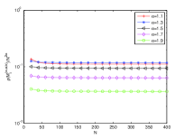
(a) $M_{i}^{(\alpha,a,b)}=M_{C,L}^{(\alpha,0,0)}$.

(b) $M_{i}^{(\alpha,a,b)}=M_{C,R}^{(\alpha,0,0)}$.

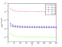
(c) $M_{i}^{(\alpha,a,b)}=M_{RL,L}^{(\alpha,0,0)}$.

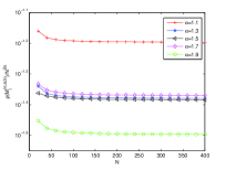
(d) $M_{i}^{(\alpha,a,b)}=M_{RL,R}^{(\alpha,0,0)}$.

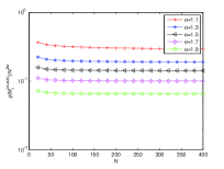
(e) $M_{i}^{(\alpha,a,b)}=M_{RC}^{(\alpha,0,0)}$.

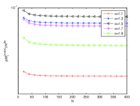
(f) $M_{i}^{(\alpha,a,b)}=M_{RZ}^{(\alpha,0,0)}$.

Figure 1: The boundedness of $\rho\left(M_{i}^{(\alpha,a,b)}\right)/N^{2\alpha}$ for $a=b=0$.

(a) $M_{i}^{(\alpha,a,b)}=M_{C,L}^{(\alpha,-\frac{1}{2},-\frac{1}{2})}$.

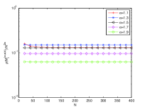
(b) $M_{i}^{(\alpha,a,b)}=M_{C,R}^{(\alpha,-\frac{1}{2},-\frac{1}{2})}$.

(c) $M_{i}^{(\alpha,a,b)}=M_{RL,L}^{(\alpha,-\frac{1}{2},-\frac{1}{2})}$.

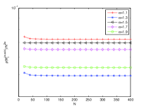
(d) $M_{i}^{(\alpha,a,b)}=M_{RL,R}^{(\alpha,-\frac{1}{2},-\frac{1}{2})}$.

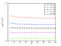
(e) $M_{i}^{(\alpha,a,b)}=M_{RC}^{(\alpha,-\frac{1}{2},-\frac{1}{2})}$.

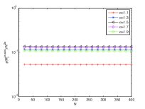
(f) $M_{i}^{(\alpha,a,b)}=M_{RZ}^{(\alpha,-\frac{1}{2},-\frac{1}{2})}$.

Figure 2: The boundedness of $\rho\left(M_{i}^{(\alpha,a,b)}\right)/N^{2\alpha}$ for $a=b=-\frac{1}{2}$.

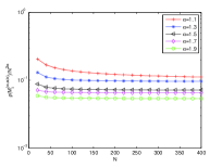
(a) $M_{i}^{(\alpha,a,b)}=M_{C,L}^{(\alpha,-\frac{1}{2},\frac{1}{2})}$.

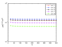
(b) $M_{i}^{(\alpha,a,b)}=M_{C,R}^{(\alpha,-\frac{1}{2},\frac{1}{2})}$.

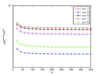
(c) $M_{i}^{(\alpha,a,b)}=M_{RL,L}^{(\alpha,-\frac{1}{2},\frac{1}{2})}$.

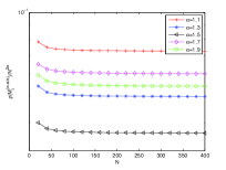
(d) $M_{i}^{(\alpha,a,b)}=M_{RL,R}^{(\alpha,-\frac{1}{2},\frac{1}{2})}$.

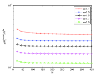
(e) $M_{i}^{(\alpha,a,b)}=M_{RC}^{(\alpha,-\frac{1}{2},\frac{1}{2})}$.

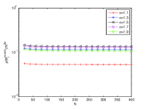
(f) $M_{i}^{(\alpha,a,b)}=M_{RZ}^{(\alpha,-\frac{1}{2},\frac{1}{2})}$.

Figure 3: The boundedness of $\rho\left(M_{i}^{(\alpha,a,b)}\right)/N^{2\alpha}$ for $a=-\frac{1}{2},b=\frac{1}{2}$.

Remark 3.2

If $\alpha$ is reduced to a positive integer, i.e., $\alpha=m$, then the matrices $M_{i}^{(\alpha,a,b)}$ are reduced the classical differential matrix $D^{(m,a,b)}$.

Remark 3.3

If the Jacobi-Gauss or Jacobi-Gauss-Radau collocation points are chosen, then we can similarly derive the corresponding differential matrices as ${}_{C}{{D}}^{(a,b,\alpha)}_{L}$, ${}_{C}{{D}}^{(a,b,\alpha)}_{R}$, ${}_{RL}{{D}}^{(a,b,\alpha)}_{L}$, and ${}_{RL}{{D}}^{(a,b,\alpha)}_{R}$. One just need to replace $c_{k,j}$ defined by (32) with

$$c_{k,j}=\frac{P_{k}^{a,b}(x_{j})\omega_{j}}{\gamma_{k}^{a,b}},{\qquad}k=0,1,...,N$$

to obtain the corresponding results [32].

4 Applications

In this section, we illustrate how to use the fractional differential matrices developed in the previous section to solve fractional differential equations.

Application to the fractional ordinary differential equation: Consider the following Baglay–Torvic equation

$$u{{}^{\prime\prime}}(x)+b(x){}_{C}D^{\alpha}_{x_{a},x}u(x)+c(x)u(x)=f(x),\quad x\in(x_{a},x_{b}),\quad\alpha\in(1,2)$$ (47)

with the conditions

• $u(x_{a})=\varphi_{a},{\quad}u^{\prime}(x_{a})=\varphi^{\prime}_{a}$;

• $u(x_{a})=\varphi_{a},{\quad}u(x_{b})=\varphi_{b}$.

Suppose that $\hat{x}_{j}\,(j=0,1,...,x_{N})$ are JGL points on the interval $[-1,1]$. Then the corresponding JGL points $x_{j}\in[x_{a},x_{b}]$ can be obtained as

$$x_{j}=\frac{(x_{b}-x_{a})\hat{x}_{j}+x_{a}+x_{b}}{2}.$$

Assume that $u_{N}=u_{N}(x)=\sum_{j=0}^{N}\hat{u}_{j}F_{j}(x)$ is the approximation of $u(x),x\in[x_{a},x_{b}]$. Then we replace $u(x)$ in (47) with $u_{N}(x)$ and let $x=x_{j}\,(j=1,2,...,N-1)$, which yields

$$(u_{N}(x)){{}^{\prime\prime}}(x_{j})+\left[{}_{C}D^{\alpha}_{x_{a},x}u_{N}(x)\right]_{x=x_{j}}+u_{N}(x_{j})=f(x_{j}).$$ (48)

Note that

$${}_{C}D^{\alpha}_{x_{a},x}u_{N}(x)=\left(\frac{x_{b}-x_{a}}{2}\right)^{-\alpha}{}_{C}D^{\alpha}_{-1,\hat{x}}u_{N}(\hat{x}).$$ (49)

Hence we can obtain from (35), (36), and (49)

$$\left(\begin{array}[]{c}{}_{C}D_{-1,\hat{x}_{0}}^{\alpha}u_{N}(\hat{x}_{0})\\ {}_{C}D_{-1,\hat{x}_{1}}^{\alpha}u_{N}(\hat{x}_{1})\\ \vdots\\ {}_{C}D_{-1,\hat{x}_{N}}^{\alpha}u_{N}(\hat{x}_{N})\end{array}\right)=\left({}_{C}{D}^{(a,b,\alpha)}_{L,x_{a},x_{b}}\right)(\hat{u}_{0},\hat{u}_{1},\cdots,\hat{u}_{N})^{T},$$ (50)

where ${}_{C}{D}^{(a,b,\alpha)}_{L,x_{a},x_{b}}\in\mathbb{R}^{(N+1)\times(N+1)}$ satisfying

$${}_{C}{D}^{(a,b,\alpha)}_{L,x_{a},x_{b}}=\left(\frac{x_{b}-x_{a}}{2}\right)^{-\alpha}\left({}_{C}{D}^{(a,b,\alpha)}_{L}\right),$$ (51)

with ${}_{C}{D}^{(a,b,\alpha)}_{L}$ defined by (36).

Combing the initial condition (I) in (47) and (50), we derive the following linear system

$$A^{(\alpha,a,b)}\mathbf{\hat{u}}=\mathbf{f},$$ (52)

where $\mathbf{f}=(f({x}_{1}),f({x}_{2}),...,f({x}_{N-1}),\varphi_{a}^{\prime})^{T}$, $\mathbf{\hat{u}}=(\hat{u}_{0},\hat{u}_{1},...,\hat{u}_{N})$, $\hat{u}_{0}=u(0)=\varphi_{a}$ is known, and $A^{(\alpha,a,b)}\in\mathbb{R}^{N\times(N+1)}$ satisfying

$$\left(A^{(\alpha,a,b)}\right)_{i-1,j}=\left({}_{C}{D}^{(a,b,2)}_{L,x_{a},x_{b}}\right)_{i,j}+b(x_{i})\left({}_{C}{D}^{(a,b,\alpha)}_{L,x_{a},x_{b}}\right)_{i,j}+c(x_{i})(E)_{i,j},{\quad}i=1,2,...,N-1,j=0,1,...N,$$

$$\left(A^{(\alpha,a,b)}\right)_{N-1,j}=\left({}_{C}{D}^{(a,b,1)}_{L,x_{a},x_{b}}\right)_{0,j}=\left(\frac{x_{b}-x_{a}}{2}\right)^{-1}\left({D}^{(a,b,1)}\right)_{0,j},{\quad}j=0,1,...,N,$$

in which $E$ is an ${(N+1)\times(N+1)}$ identity matrix and ${D}^{(a,b,1)}$ is the first-order differential matrix.

If we use the boundary conditions (II) in (47), we can obtain the following linear system

$$A^{(\alpha,a,b)}\mathbf{\hat{u}}=\mathbf{f},$$ (53)

where $\mathbf{f}=(f({x}_{1}),f({x}_{2}),...,f({x}_{N-1}))^{T}$, $\mathbf{\hat{u}}=(\hat{u}_{0},\hat{u}_{1},...,\hat{u}_{N})$, $\hat{u}_{0}=u(x_{a})=\varphi_{a}$ and $\hat{u}_{N}=u(x_{b})=\varphi_{b}$ are known, and $A^{(\alpha,a,b)}\in\mathbb{R}^{(N-1)\times(N+1)}$ satisfying

$$\left(A^{(\alpha,a,b)}\right)_{i-1,j}=\left({}_{C}{D}^{(a,b,2)}_{L,x_{a},x_{b}}\right)_{i,j}+b(x_{i})\left({}_{C}{D}^{(a,b,\alpha)}_{L,x_{a},x_{b}}\right)_{i,j}+c(x_{i})(E)_{i,j},{\quad}i=1,2,...,N-1,j=0,1,...,N.$$

Application to the fractional partial differential equations: Consider the following fractional diffusion equation

$$\left\{\begin{aligned} &\frac{\partial u}{\partial t}=c_{+}(x){}_{RL}D_{x_{a},x}^{\alpha}u(x,t)+c_{-}(x){}_{RL}D_{x,x_{b}}^{\alpha}u(x,t)+f(x,t),{\quad}(x,t){\,\in\,}(x_{a},x_{b}){\times}(0,T],T>0,\\ &u(x,0)=\phi_{0}(x),{\quad}x{\,\in\,}[x_{a},x_{b}],\\ &u(x_{a},t)=\varphi_{a}(t),{\quad}u(x_{b},t)=\varphi_{b}(t){\quad}t{\,\in\,}\partial{\Omega}\times(0,T],\end{aligned}\right.$$ (54)

Assume that $u_{N}(x,t)$ be an $N$th-order polynomial with respect $x$ for fixed $t$, $x_{j}\,(j=0,1,...,N)$ are the JGL collocation points on $[x_{a},x_{b}]$. Inserting $u_{N}(x,t)$ into (54) and letting $x=x_{j}\,(j=1,2,..,N-1)$ yield

$$\frac{\mathrm{d}u_{N}(x_{j},t)}{\,{\rm d}t}=c_{+}(x_{j}){}_{RL}D_{x_{a},x_{j}}^{\alpha}u_{N}(x_{j},t)+c_{-}(x_{j}){}_{RL}D_{x_{j},x_{b}}^{\alpha}u_{N}(x_{j},t)+f(x_{j},t).$$ (55)

As is done for the fractional ordinary differential equations, we can obtain the matrix representation of (55) below

$$\frac{\mathrm{d}\mathbf{\hat{u}}(t)}{\,{\rm d}t}=A^{(\alpha,a,b)}\mathbf{\hat{u}}(t)+\mathbf{f}(t).$$ (56)

where $\mathbf{\hat{u}}(t)=(u_{N}(x_{0},t),u_{N}(x_{1},t),...,u_{N}(x_{N},t))^{T}$, $u_{N}(x_{0},t)=\varphi_{a}(t)$ and $u_{N}(x_{N},t)=\varphi_{b}(t)$ are known functions, $\mathbf{f}(t)=(f(x_{1},t),f(x_{2},t),...,f(x_{N-1},t))^{T}$, and $A^{(\alpha,a,b)}\in\mathbb{R}^{(N-1)\times(N+1)}$ satisfying

$$\left(A^{(\alpha,a,b)}\right)_{i-1,j}= \left(\frac{x_{b}-x_{a}}{2}\right)^{-\alpha}\left[c_{+}(x_{i})\left({}_{RL}{D}^{(a,b,\alpha)}_{L}\right)_{i-1,j}+c_{-}(x_{i})\left({}_{RL}{D}^{(a,b,\alpha)}_{R}\right)_{i,j}\right],$$

$$i=1,2,...,N-1,j=0,1,...,N,$$

in which the matrices ${}_{RL}{D}^{(a,b,\alpha)}_{L}$ and ${}_{RL}{D}^{(a,b,\alpha)}_{R}$ are defined by (39) and (41), respectively. From (54), the initial condition of (56) can be given as follows

$$\mathbf{\hat{u}}(0)=(\phi_{0}(x_{0}),\phi_{0}(x_{1}),...,\phi_{0}(x_{N}))^{T}.$$ (57)

Now, the fractional ordinary system (56) with initial condition (57) can be solved by any known methods as the Euler method, the trapezoidal rule, linear multi-step methods, Runge-Kutta methods, and so on. In the numerical simulation, we use the trapezoidal rule to solve (56).

5 Numerical examples

This section provides the numerical examples to verify the methods obtained in the preceding sections.

Example 5.1

Consider the following Baglay-Torvik equation [9, 26]

$$u{{}^{\prime\prime}}(x)+{}_{C}D^{\alpha}_{0,x}u(x)+u(x)=f(x),\quad x\in(0,1],{\quad}1<\alpha<2,$$ (58)

with the initial conditions

$$u(0)=0,\quad u^{\prime}(0)=w.$$ (59)

Choosing appropriate $f(x)$ such that (58) has the exact solution $u(x)=\sin{wx}$.

We set $a=b=0$ (Legendre collocation method) and $a=b=-1/2$ (Chebyshev collocation method), the results are shown in Tables 1 and 2, respectively, where the maximum absolute errors of the present method (52) and the shifted Chebyshev tau (SCT) method developed in [9] are shown. From this example, we can see that our method shows more accurate results than the SCT method developed in [9].

If the initial condition $u^{\prime}(0)=w$ in (59) is replaced by $u(1)=\sin{w}$, we can obtain the boundary value problem. In such a case, we choose the suitable right hand side function $f(x)$ such that (58) has the exact solution $u(x)=\sin{wx}$. We use the method (53) to solve the this problem with $w=4\pi,\alpha=1.1,1.25,1.4,1.6,1.75,1.9$. Tables 3 and 4 display the maximum absolute errors at Legendre-Gauss-Lobatto ($a=b=0$) points and Chebyshev-Gauss-Lobatto ($a=b=-\frac{1}{2}$) points, respectively. Clearly, the satisfactory numerical results are obtained.

Table 1: The absolute errors for Example 5.1 with different $N$ and $a=b=0$, $\alpha=1.5$.

$N$	$w$	Method (52)	SCT [9]	$w$	Method (52)	SCT [9]
4	1	2.4175e-04	3.4e-04	$4\pi$	1.2516e+01	3.9e-00
8	1	7.3967e-10	4.3e-07	$4\pi$	1.3775e+00	4.7e-01
16	1	6.4948e-14	1.8e-08	$4\pi$	8.5461e-05	3.5e-05
32	1	2.3959e-13	7.1e-10	$4\pi$	4.5841e-12	1.4e-06
48	1	3.0032e-13	9.9e-11	$4\pi$	2.3109e-12	1.9e-07
64	1	1.5175e-12	2.4e-11	$4\pi$	1.0300e-11	4.8e-08

Table 2: The absolute errors for Example 5.1 with different $N$ and $a=b=-1/2$, $\alpha=1.5$.

$N$	$w$	Method (52)	SCT [9]	$w$	Method (52)	SCT [9]
4	1	1.3548e-04	3.4e-04	$4\pi$	1.1894e+01	3.9e-00
8	1	2.8661e-10	4.3e-07	$4\pi$	4.8230e-01	4.7e-01
16	1	5.3291e-15	1.8e-08	$4\pi$	2.3177e-05	3.5e-05
32	1	2.7367e-13	7.1e-10	$4\pi$	1.2018e-12	1.4e-06
48	1	2.4891e-13	9.9e-11	$4\pi$	4.5565e-12	1.9e-07
64	1	4.4387e-13	2.4e-11	$4\pi$	7.8381e-12	4.8e-08

Table 3: The absolute errors for Example 5.1 with boundary value conditions and $a=b=0$, $w=4\pi$.

$N$	$\alpha=1.1$	$\alpha=1.25$	$\alpha=1.4$	$\alpha=1.6$	$\alpha=1.75$	$\alpha=1.9$
8	2.4934e-01	2.1828e-01	1.8398e-01	1.4161e-01	1.1189e-01	7.0096e-02
12	4.4902e-03	3.8408e-03	3.1023e-03	2.1753e-03	1.5838e-03	8.9844e-04
16	1.5053e-05	1.2813e-05	1.0230e-05	6.9318e-06	4.8828e-06	2.7329e-06
20	1.6351e-08	1.3898e-08	1.1044e-08	7.3458e-09	5.0633e-09	2.8151e-09
24	7.5480e-12	6.2294e-12	5.1675e-12	3.1971e-12	1.4853e-12	2.6823e-12
28	2.7034e-13	2.5047e-13	4.1245e-13	8.9195e-13	4.8161e-13	3.4023e-13

Table 4: The absolute errors for Example 5.1 with boundary value conditions and $a=b=-\frac{1}{2}$, $w=4\pi$.

$N$	$\alpha=1.1$	$\alpha=1.25$	$\alpha=1.4$	$\alpha=1.6$	$\alpha=1.75$	$\alpha=1.9$
8	1.2224e-01	1.1248e-01	1.0122e-01	8.6472e-02	7.5269e-02	5.8414e-02
12	1.4914e-03	1.3028e-03	1.0830e-03	7.9562e-04	6.0160e-04	3.7026e-04
16	4.2450e-06	3.6549e-06	2.9657e-06	2.0617e-06	1.4783e-06	8.5876e-07
20	4.1101e-09	3.5201e-09	2.8283e-09	1.9126e-09	1.3308e-09	7.6665e-10
24	1.6886e-12	1.2088e-12	1.4165e-12	1.3994e-12	5.8165e-13	3.7370e-13
28	2.3892e-13	8.9373e-14	6.9333e-13	3.6260e-13	5.0826e-13	1.1949e-12

Example 5.2

Consider the following diffusion equation [3]

$$\left\{\begin{aligned} &\frac{\partial u}{\partial t}={}_{RZ}D_{x}^{\alpha}u(x,t)+f(x,t),{\quad}(x,t){\,\in\,}(0,1){\times}(0,T],T>0,\\ &u(x,0)=x^{2}(1-x^{2}),{\quad}x{\,\in\,}[0,1],\\ &u(0,t)=u(1,t)=0{\quad}t{\,\in\,}\partial{\Omega}\times(0,T].\end{aligned}\right.$$ (60)

Choosing the suitable right hand side function $f(x,t)$ such that (60) has the following exact solution

$$u(x,t)=(t+1)^{\alpha}x^{2}(1-x)^{2}.$$

Since the exact solution is a polynomial of order 4, so we choose $N=4$ in the computation. The time step size ($\tau=10^{-2}$) is the same as that in [3], the fractional orders are chosen as $\alpha=1.1,1.3,1.5,1.7,1.9$, the absolute maximum errors are shown in Table 5. The notation $(a,b)=(0,0)$ means the method (56)–(57) with $a=b=0$ is used to solve (60), which is the same for $(a,b)=(-\frac{1}{2},-\frac{1}{2})$ and $(a,b)=(-\frac{1}{2},\frac{1}{2})$. $N=100$ and $N=200$ in Table 5 imply the space step size $h=1/N$ was used in [3]. Obviously, the present methods show better numerical solutions here.

Table 5: The absolute errors for Example 5.2 at $t=10$.

Methods	$\alpha=1.1$	$\alpha=1.3$	$\alpha=1.5$	$\alpha=1.7$	$\alpha=1.9$
$(a,b)=(0,0)$	1.0120e-8	5.7515e-8	1.7774e-7	4.5405e-7	1.0518e-6
$(a,b)=(-\frac{1}{2},-\frac{1}{2})$	1.0116e-8	5.7501e-8	1.7772e-7	4.5402e-7	1.0518e-6
$(a,b)=(-\frac{1}{2},\frac{1}{2})$	9.6527e-9	5.4857e-8	1.6953e-7	4.3308e-7	1.0032e-6
CN [3]($N=100$)	7.5271e-5	1.6136e-4	3.5410e-4	8.0486e-4	1.9026e-3
CN [3]($N=200$)	2.0479e-5	3.8070e-5	8.3236e-5	1.9120e-4	4.6505e-4

6 Conclusion

In this paper, we derive the fractional differential matrices with respect to the Jacobi-Gauss points. The spectral radius of the derived fractional differential matrices are numerically investigated, which show the behaviors as (46). We also develop the spectral collocation schemes to solve the fractional differential equations, which show good performances. Tian and Deng [36] also developed the fractional differential matrices, but their method will blow up when performing on the computers with double precision with $N$ being suitably large, i.e., when $N>35$, the results are not believable, see Remark 1 in [36]. Clearly, our method is more stable than that in [36], which is also tested by the numerical examples in the present paper, where all the numerical results are computed on the computer with double precision by Matlab.

References

- [1] C. Canuto, M. Y. Hussaini, A. Quarteroni, T. A. Zang, Specral Methods: fundamentals in Single Domains, Springer-Verlag, Berlin (2006).
- [2] J. Cao, C. Xu, A high order schema for the numerical solution of the fractional ordinary differential equations, J. Comput. Phys. 238 (2013) 154–168.
- [3] C. Çelik, M. Duman, Crank-Nicolson method for the fractional diffusion equation with the Riesz fractional derivative, J. Comput. Phys. 231 (2012) 1743–1750.
- [4] F. Chen, Q.W. Xu, J. S Hesthaven, A multi-domain spectral method for time-fractional differential equations, http://infoscience.epfl.ch/record/191320.
- [5] K. Diethelm, N. J. Ford, A. D. Freed, Detailed error analysis for a fractional Adams method, Numer. Algor. 36 (2004) 31–52.
- [6] K. Diethelm, N. J. Ford, A. D. Freed, Y. Luchko, Algorithms for the fractional calculus: a selection of numerical methods, Comput. Methods Appl. Mech. Engrg. 194 (2005) 43–773.
- [7] F. Cortés, M. Elejabarrieta, Finite element formulations for transient dynamic analysis in structural systems with viscoelastic treatments containing fractional derivative models, Int. J. Numer. Meth. Engng. 69 (2007) 2173–2195.
- [8] E. H. Doha, A. H. Bhrawy, S. S. Ezz-Eldien, A chebyshev spectral method based on operational matrix for initial and boundary value problems of fractional order, Comput. Math. Appl. 62 (2011) 2364–2373.
- [9] E. H. Doha, A. H. Bhrawy, S. S. Ezz-Eldien, Efficient chebyshev spectral methods for solving multi-term fractional orders differential equations, Appl. Math. Modelling 35 (2011) 5662–5672.
- [10] E. H. Doha, A.H. Bhrawy, S.S. Ezz-Eldien, A new Jacobi operational matrix: An application for solving fractional differential equations, Appl. Math. Modelling 36 (2012) 4931–4943.
- [11] S. Esmaeili, M. Shamsi, A pseudo-spectral scheme for the approximate solution of a family of fractional differential equations, Commun. Nonlinear Sci. Numer. Simulat. 16 (2011) 3646–3654.
- [12] Z. Gao, X. Z. Liao, Discretization algorithm for fractional order integral by Haar wavelet approximation, Appl. Math. Comput. 218 (2011) 1917–1926.
- [13] G. H. Gao, Z. Z. Sun, H. W. Zhang, A new fractional numerical differentiation formula to approximate the Caputo fractional derivative and its applications, J. Comput. Phys. 259 (2014) 33–50.
- [14] V. V. Kulish, Application of fractional calculus to fluid mechanics, J. Fluids Eng. 124 (2002) 803–808.
- [15] P. Kumar, Om P. Agrawal, An approximate method for numerical solution of fractional differential equations, Signal Processing 86 (2006) 2602–2610.
- [16] M. Lakestani, M. Dehghan, S. Irandoust-pakchin, The construction of operational matrix of fractional derivatives using B-spline functions, Commun. Nonlinear Sci. Numer. Simulat. 17 (2012) 1149–1162.
- [17] T. A. M. Langlands, B. I. Henry, The accuracy and stability of an implicit solution method for the fractional diffusion equation, J. Comput. Phys. 205 (2005) 719–736.
- [18] C. P. Li, A. Chen, J. J. Ye, Numerical approach to fractional calculus and fractional ordinary differential equations, J. Comput. Phys. 230 (2011) 3352–3368.
- [19] C. P. Li, F. H. Zeng, and F. Liu, Spectral approximations to the fractional integral and derivative, Fract. Calc. Appl. Anal. 15 (2012) 383–406.
- [20] C. P. Li, Z. G. Zhao, Y. Q. Chen, Numerical approximation of nonlinear fractional differential equations with subdiffusion and superdiffusion, Comput. Math. Appl. 62 (2011) 855–875.
- [21] F. Liu, Q. Q. Yang, I. Turner, Two new implicit numerical methods for the fractional cable equation, J. Comput. Nonlinear Dyn. 6 (2011) 011009–1.
- [22] C. Lubich, Discretized fractional calculus, SlAM J. Math. Anal. 17 (1986) 704–719.
- [23] V. E. Lynch, B. A. Carreras, D. del-Castillo-Negrete, K. M. Ferreira–Mejias, H. R. Hicks, Numerical methods for the solution of partial differential equations of fractional order, J. Comput. Phys. 192 (2003) 406–42.
- [24] D. A. Murio, On the stable numerical evaluation of Caputo fractional derivatives, Comput. Math. Appl. 51 (2006) 1539–1550.
- [25] K. Oldham, J. Spanier, The Fractional Calculus: Integrations and Differentiations to Arbitrary Order, Acdemic Press, New York, 1974.
- [26] I. Podlubny, Fractional Differential Equations, Acdemic Press, San Dieg, 1999.
- [27] I. Podlubny, Matrix approach to discrete fractional calculus, Fract. Calc. Appl. Anal. 3 (2000) 359–386.
- [28] I. Podlubny, A. Chechkin, T. Skovranek, Y. Q. Chen, B. Vinagre, Matrix approach to discrete fractional calculus II: partial fractional differential equations, J. Comput. Phys. 228 (2009) 3137–3153.
- [29] Y. A. Rossikhin, M. V. Shitikova, Application of fractional calculus for dynamic problems of solid mechanics: Novel trends and recent results, Applied Mechanics Reviews 63 (2010) 010801–1.
- [30] A. Saadatmandi, M. Dehghan, A new operational matrix for solving fractional-order differential equations, Comput. Math. Appl. 59 (2010) 1326–1336.
- [31] S. G. Samko, A. A. Kilbas, O. I. Marichev, Fractional Integrals and Derivatives, Gordon and breach Science, Yverdon, Switzerland, 1993.
- [32] J. Shen, T. Tang, and L. L. Wang, Spectral Methods: Algorithms, Analysis and Applications, Springer, New York, 2011.
- [33] E. Sousa, How to approximate the fractional derivative of order , International Journal of Bifurcation and Chaos, 22 (2012) Article ID: 1250075.
- [34] H. Sugiura, T. Hasegawa, Quadrature rule for Abel’s equations: Uniformly approximating fractional derivatives, J. Comput. Appl. Math. 223 (2009) 459–468.
- [35] Z. Z. Sun, X. N. Wu, A fully discrete difference scheme for a diffusion-wave system, Appl. Numer. Math. 56 (2006) 193–209.
- [36] W. Y. Tian, W. H. Deng, Y. J. Wu, Polynomial spectral collocation method for space fractional advection-diffusion equation, Numer. Methods P. D. Equ. 30 (2014) 514–535.
- [37] W. Y. Tian, H. Zhou, W. H. Deng, A class of second order difference approximations for solving space fractional diffusion equations, http://arxiv.org/abs/1201.5949.
- [38] Q. W. Xu, J. S. Hesthaven, Stable multi-domain spectral penalty methods for fractional partial differential equations, J. Comput. Phys. 257 (2014) 241–258.
- [39] Q. Yu, F. Liu, V. Anh, I. Turner, Solving linear and nonlinear space-time fractional reaction-diffusion equations by the Adomian decomposition method, Int. J. Numer. Meth. Engng. 74, (2008) 138–158.
- [40] Z. M. Odibat, Approximations of fractional integrals and Caputo fractional derivatives, Appl. Math. Comput. 178 (2006) 527–533.
- [41] Z. M. Odibat, Computational algorithms for computing the fractional derivatives of functions, Math. Comput. Simulat. 79 (2009) 2013–2020.
- [42] P. Zhuang, T. Gu, F. Liu, I. Turner, P. K. D. V. Yarlagadda, Time-dependent fractional advection-diffusion equations by an implicit MLS meshless method, Int. J. Numer. Meth. Engng. 88 (2011) 1346–1362.