MCnet-14-10

$\mathrm{(MC)}^{3}$– a Multi-Channel Markov Chain Monte Carlo algorithm for phase-space sampling

Abstract

A new Monte Carlo algorithm for phase-space sampling, named $\mathrm{(MC)}^{3}$, is presented. It is based on Markov Chain Monte Carlo techniques but at the same time incorporates prior knowledge about the target distribution in the form of suitable phase-space mappings from a corresponding Multi-Channel Importance Sampling Monte Carlo. The combined approach inherits the benefits of both techniques while typical drawbacks of either solution get ameliorated.

1 Introduction

The stochastic generation of samples from a positive definite probability density defined over some high-dimensional phase space poses a challenge in many fields of research. This problem is most naturally addressed by Monte Carlo methods. In particle physics, Monte Carlo event generators are used to make theoretical predictions for the outcome of scattering experiments for example at the Large Hadron Collider [1].

Such Monte Carlo generators sample the accessible multi-particle phase space to generate individual events with a probability density given by squared transition amplitudes. In turn, fully differential production rates, corresponding to arbitrary final-state observables, can be evaluated. Triggered by the experimental needs and theoretical breakthroughs, amplitude calculations for higher and higher final-state particle multiplicities became available over the last years. While tree-level matrix element calculations can be considered fully automated, see e.g. Refs. [2, 3, 4, 5, 6, 7], the emerging standard even for high-multiplicity final states is next-to-leading-order accuracy in the strong coupling, see e.g. Refs. [8, 9, 10, 11, 12, 13, 14]. In practice, the actual calculations are often organized and performed in event generation frameworks such as Helac [15], MadGraph [7] or SHERPA ​​ [16, 17] that implement the cross section integration and event generation.

Given the calculational costs for evaluating a complicated $2\to n$ scattering amplitude, efficient phase-space generation is of utmost importance. With the high level of optimization that has gone into amplitude calculations, improvements in phase-space sampling are the most promising lever arm to further improve existing parton-level event generators. The existing programs all rely on adaptive Monte Carlo integration techniques based on Importance Sampling. Most commonly used is the adaptive Multi-Channel Importance Sampling (IS) approach [18, 3, 19, 20]. Alternatively, or in combination, methods inspired by the Vegas algorithm [21] are also available [22, 23, 24, 25].

The construction of suitable phase-space mappings for a Multi-Channel integrator requires detailed knowledge about the target function to sample from as it needs to be approximated as good as possible over the entire phase space. This is typically achieved by analysing the topology of the contributing scattering amplitudes. There exist known mappings for essentially all resonance and enhancement structures occurring in individual topologies. However, due to non-trivial phase-space restrictions, interference effects or competing resonances, the multi-channel integrator is never fully efficient. In particular for processes with many final-state particles these deficiencies can accumulate and dramatically reduce the overall sampling efficiency.

An alternative class of algorithms for creating samples according to a probability density is Markov Chain Monte Carlo (MCMC), see e.g. Ref. [26] and references therein. These algorithms are used in a variety of research fields, e.g., astrophysics, biology and statistical physics. So far, their usage in high-energy particle physics is rather limited. Examples are the calculation of cross-sections by integration over multi-dimensional phase spaces [27], the generation of unweighted events in next-to-leading order QCD calculations [28] or the mapping of sets of measurements onto high-dimensional parameter spaces [29, 30]. The most well-known MCMC algorithm is the Metropolis–Hastings algorithm [31, 32]. A large variety of advanced algorithms exist, in particular for multimodal problems, see e.g. Refs. [33, 34, 35, 36, 37].

In this paper, we present a new sampling algorithm which combines the prior knowledge of Multi-Channel Importance Sampling with the flexibility of the Metropolis–Hastings algorithm. We apply the algorithm to three concrete examples and study the properties of the samples produced. The first example is an abstract problem and corresponds to the extreme case where the modelling of the target function is missing a resonant feature. The second example deals with the generation of Monte Carlo events for Drell-Yan production serving as a first illustration of our main application for the new algorithm. In our third example we briefly present an implementation of the algorithm in the SHERPA ​​event generator and study its performance in the generation of unweighted events for Drell-Yan plus multijet production under LHC conditions.

The paper is structured as follows: we first review the well-known Multi-Channel Importance Sampling and the Metropolis–Hastings algorithm in Section 2 where we also introduce our new algorithm. Section 3 shows three extended examples for the application of this algorithm, followed by a discussion about its advantages and disadvantages. The paper concludes in Section 4.

2 Sampling algorithms

A standard task in computational physics is the generation of a sample of random variables distributed according to a normalized target function $f(x)$. In this section we describe two well-known and complementary approaches to that problem – namely, Importance Sampling Monte Carlo, and in particular Multi-Channel Importance Sampling, as well as Markov Chain Monte Carlo. We lay out a new method that attempts to combine the respective advantages of both techniques.

2.1 Multi-Channel Importance Sampling

The generation of samples $\{x_{\_}{i}\}~{}(i=1,\dots,N)$ according to a function $f$ is a byproduct of Monte Carlo integration. Consider the evaluation of the $d-$dimensional finite integral $\mathcal{I}=\int_{\_}{\Omega_{\_}d}f(x)\,\textup{d}x$, with $x\in\mathbbm{R}^{d}$, over the non-negative target function $f$ in the integration volume $V=\,\textup{Vol}(\Omega_{\_}d)$. The Monte Carlo estimate for this integral is given through

$${\hat{\mathcal{I}}}_{\_}N=\frac{V}{N}\sum\limits_{\_}{i=1}^{N}f(x_{\_}i)=V\bar{f}\,,$$ (1)

and an estimate of the corresponding uncertainty is given by

$$\hat{\sigma}_{\_}{\mathcal{I}_{\_}N}=V\frac{\hat{\sigma}_{\_}N[f]}{\sqrt{N}}\,,\;\;\text{with}\quad\hat{\sigma}_{\_}N[f]=\sqrt{\hat{V}[f]}=\sqrt{\frac{1}{N-1}\sum_{\_}{i=1}^{N}(f(x_{\_}i)-\bar{f})^{2}}\,,$$ (2)

where $\hat{\sigma}[f]$ and $\hat{V}[f]$ denote the estimates for the standard deviation and variance of $f$, respectively.

Variance reduction techniques attempt to minimize the uncertainty estimate by generating a set of points that follow the distribution $f(x)$ as closely as possible. For a pedagogical introduction see e.g. Refs. [38, 39]. To illustrate this technique, we consider a change of the integration variables

$$\mathcal{I}=\int_{\_}{\Omega_{\_}d}f(x)\,\textup{d}x=\int_{\_}{\Omega_{\_}d}\frac{f(x)}{g(x)}g(x)\,\textup{d}x=\int_{\_}{\Omega_{\_}d}\frac{f(x)}{g(x)}\,\textup{d}G(x)\,,$$ (3)

where $g(x)$ approximates the target function $f(x)$ and is referred to as mapping. We require $g(x)$ to be non-negative, i.e. $g(x)\geq 0$, and normalizable. We further assume that there exists an efficient random number generator for samples $\{x_{\_}i\}$ according to the cumulative distribution function $G(x)$, e.g. using the inverse transformation method [38]. It can be shown that for suitably chosen $g(x)$ the estimate of the uncertainty of $\hat{\mathcal{I}}_{\_}N$,

$$\hat{\sigma}_{\_}{\mathcal{I}_{\_}N}=V\frac{\hat{\sigma}_{\_}N\left[f/g\right]}{\sqrt{N}}\,,$$ (4)

can be significantly reduced. The resulting set of points $\{x_{\_}{i}\}$ is distributed according to the cumulative distribution $G(x)$, and each point carries a weight $w(x_{\_}{i})=f(x_{\_}{i})/g(x_{\_}{i})$. The weighted distribution then resembles the function $f$. The events can be unweighted using, e.g., an acceptance-rejection method [40].

The outlined method can be generalized to the case where $g(x)$ resembles a sum of $m$ individual mappings, or channels, $g_{\_}k(x)~{}(k=1,\dots,m)$, i.e.

$$g(x)=\sum_{\_}{k=1}^{m}\alpha_{\_}kg_{\_}k(x)\,,\;\;\text{with}\quad\alpha_{\_}k\in[0,1]\;\;\text{and}\;\;\sum_{\_}{k=1}^{m}\alpha_{\_}k=1\,.$$ (5)

All $g_{\_}k(x)$ shall have the same properties as the original function $g(x)$ discussed above, in particular all cumulants $G_{\_}k(x)$ need to be known and invertible. The uncertainty estimate for the integral depends on the choice of the channel weights $\alpha_{\_}k$. In fact, the variance of $f/g$ can be minimized by adapting the channel weights starting from an initial assignment during a training integration phase [41]. This decomposition approach is often referred to as Multi-Channel Importance Sampling.

As typical for an importance sampling technique, it relies on prior knowledge about the target function $f$ in terms of the approximation $g$, respectively the individual channels $g_{\_}k$. With an optimal choice for the set of channels the variance of $f/g$ might even vanish completely; this, however, corresponds to the case that the problem is solved exactly. In realistic scenarios $f$ can only be approximated and one is left with a non-vanishing variance. In particular the unweighting efficiency for generated phase-space points is very sensitive to the quality of the approximation $g(x)$ to account for all pronounced features of the target distribution. Missing a local structure of $f$ can significantly reduce the global unweighting efficiency. In practical calculations this can require a huge proliferation of channels to be considered, rendering their adaptation and steering computationally challenging. Let us note that, in contrast to the Markov Chain method discussed next, the phase-space points $x_{\_}i$ generated with Importance Sampling Monte Carlo are statistically independent, so free of any autocorrelation.

2.2 Markov Chain Monte Carlo

An alternative way to generate random numbers according to a target function $f(x)$ is to use Markov Chain Monte Carlo. This procedure generates a Markov Chain, i.e. a sequence of random values $X_{\_}{k}$ for which the next element, $X_{\_}{k+1}$, only depends on the current state,

$$P(X_{\_}{k+1}=x|X_{\_}{1}=x_{\_}{1},X_{\_}{2}=x_{\_}{2},\dots,X_{\_}{k}=x_{\_}{k})=P(X_{\_}{k+1}=x|X_{\_}{k}=x_{\_}{k})\,.$$ (6)

A Markov Chain is said to be time-homogeneous if $P(X_{\_}{k+1}=x|X_{\_}{k}=x_{\_}{k})$ is the same for all $k$. A time-homogeneous Markov Chain can be shown to have a unique stationary distribution $f(x)$. If, in addition, the Markov Chain is aperiodic, recurrent and irreducible it is also ergodic, i.e. its limiting probability to reach a certain state does not depend on the initial condition, or starting value.

The first and probably best known MCMC algorithm is the Metropolis–Hastings algorithm [31]: for an arbitrary point $X_{\_}{k}=x$, a new point $y$ is generated according to a proposal function $g(y|x)$. The acceptance probability for this new point is

$$\alpha(y|x)=\min\left(1,\frac{f(y)g(x|y)}{f(x)g(y|x)}\right)\,.$$ (7)

Thus, the new point is accepted with a probability of $\alpha$ and so $X_{\_}{k+1}=y$ or, with a probability of $1-\alpha$, the point is rejected and $X_{\_}{k+1}=x$. The conditional probability to move from the current point $x$ to the point $y$ is $p(y|x)=\alpha(y|x)g(y|x)$ and referred to as transition kernel, $\mathcal{K}(y|x)$. For symmetric proposal functions, e.g., a Gaussian, a flat-top or a Cauchy distribution, the acceptance probability reduces to $\alpha(y|x)=\min\left(1,\frac{f(y)}{f(x)}\right)$. Since the acceptance probability fulfils the requirement of detailed balance, i.e.,

$$f(x)p(y|x)=f(x)\mathcal{K}(y|x)=f(y)\mathcal{K}(x|y)=f(y)p(x|y)\,,$$ (8)

and the process is ergodic, the resulting sequence is a Markov Chain with limiting distribution $f(x)$.

Note that the above procedure can introduce an autocorrelation between points. This can be reduced by introducing a lag, i.e. saving only every $n$th point of the Markov Chain. Also note that reasonable starting values have to be found for most applications if the number of samples is small. This can either be done by removing the first few samples from the Markov Chain (burn-in phase) or by running several chains in parallel and requiring them to mix. Practical considerations can e.g. be found in Ref. [42]. An additional obstacle are multimodal distributions for which the mixing of several chains and the convergence of a single chain to its limiting distribution can be poor.

2.3 Multi-Channel Markov Chain Monte Carlo $\mathrm{(MC)}^{3}$

Importance Sampling and MCMC suffer from complementary difficulties. In the first case, a bad mapping of the target function in only one region of phase space can cause a significant drop in efficiency for the unweighting process. In the latter case, the samples show an autocorrelation and, in addition, multimodal target distributions can cause poor mixing or convergence of the Markov chains.

We propose a combination of both sampling algorithms to Multi-Channel Markov Chain Monte Carlo, or $\mathrm{(MC)}^{3}$, which overcomes the difficulties mentioned above. The algorithm is a variant of the path-adaptive Metropolis–Hastings (PAMH) sampler proposed in Ref. [26] in a sense that we use prior analytical knowledge about the target function in a Metropolis–Hastings sampler. This information is given by the multi-channel decomposition used in importance sampling. Technically, $\mathrm{(MC)}^{3}$ mixes two transition kernels with a common limiting distribution $f(x)$.

The first transition kernel encodes the prior knowledge about the target function. Let $g_{\_}{IS}(x)$ be a probability density which approximates $f(x)$ corresponding to the multi-channel setup used in the importance sampling algorithm described earlier. Assume that efficient random number generators exist for the individual channels. The proposal function for the first transition kernel, $g_{\_}{IS}(y|x)=g_{\_}{IS}(y)$, is generated from $g_{\_}{IS}(y)=\sum_{\_}{k=1}^{m}\alpha_{\_}kg_{\_}k(y)$ and accepted with a probability

$$\alpha_{\_}{IS}(y|x)=\min\left(1,\frac{f(y)g_{\_}{IS}(x)}{f(x)g_{\_}{IS}(y)}\right)\,.$$ (9)

The resulting transition kernel is $\mathcal{K}_{\_}{IS}(y|x)=\alpha_{\_}{IS}(y|x)g_{\_}{IS}(y)$.

The second transition kernel is identical to the one used in the Metropolis–Hastings algorithm, i.e., $\mathcal{K}_{\_}{\mathrm{MH}}(y|x)=\alpha_{\_}{\mathrm{MH}}(y|x)g_{\_}{\mathrm{MH}}(y|x)$, where $g_{\_}{\mathrm{MH}}(y|x)$ is a symmetric and localized proposal distribution and the resulting acceptance rate is

$$\alpha_{\_}{\mathrm{MH}}(y|x)=\min{\left(1,\frac{f(y)}{f(x)}\right)}\,.$$ (10)

In each iteration during the MCMC algorithm, the first (or second) transition kernel is chosen with a probability of $\beta$ (or $1-\beta$), with $\beta\in[0,1]$. The combined transition kernel for the $\mathrm{(MC)}^{3}$ sampler is thus given by

$$\mathcal{K}_{\_}{\mathrm{(MC)}^{3}}(y|x)=\beta\mathcal{K}_{\_}{IS}(y|x)+(1-\beta)\mathcal{K}_{\_}{MH}(y|x).$$ (11)

The acceptance probability preserves detailed balance since

$$f(x)\mathcal{K}_{\_}{\mathrm{(MC)}^{3}}(y|x) = \beta\min{\left(f(x)g_{\_}{IS}(y|x),f(y)g_{\_}{IS}(x|y)\right)}$$

$$+(1-\beta)\min{\left(f(x)g_{\_}{MH}(y|x),f(y)g_{\_}{MH}(x|y)\right)}$$

$$= f(y)\mathcal{K}_{\_}{\mathrm{(MC)}^{3}}(x|y)$$

is symmetric in $x$ and $y$. The limiting distribution of the constructed Markov chain is $f(x)$.

The parameter $\beta$ reflects the confidence of the user in the prior information to reflect all relevant features of the target function and can be chosen freely. Values close to unity indicate that the prior knowledge has no uncertainty, i.e. all peak structures are assumed to be precisely mapped out. In contrast, a value of $\beta$ equal to zero corresponds to a pure Metropolis–Hastings algorithm without any prior knowledge.

2.4 Practical considerations for $\mathrm{(MC)}^{3}$

The $\mathrm{(MC)}^{3}$ algorithm has several free parameters which can be optimized according to the problem at hand. These are

• the probability for choosing the IS or MH transition kernel, $\beta$. This parameter controls to what extend the prior information is used;

• the $m$ channel weights, $\alpha_{\_}k$, in the IS transition kernel. These parameters model the decomposition of the mapping function $g_{\_}{\mathrm{IS}}(x)$;

• the width of the proposal function $g_{\_}{\mathrm{MH}}(y|x)$ in the MH transition kernel. This parameter has an impact on the sampling efficiency of the Metropolis–Hastings-part of the algorithm.

The optimization procedure followed for the studies presented in this paper is a sequence of three pre-runs: firstly, the channel weights of the IS transition kernel are optimized by iteratively updating channel weights. This is accomplished by comparing the target function with the mapping function using only a small set of samples, depending on the number of channels employed. Details of this adaptation strategy can be found in Ref. [41]. In consequence, some (very small) channel weights $\alpha_{\_}i$ might be switched off completely, effectively reducing the number of active channels. Secondly, the width of the proposal function of the MH transition kernel is adjusted in subsequent sets of samples such that the efficiency lies within a range of $[0.25,0.5]$. Thirdly, the $\mathrm{(MC)}^{3}$ algorithm is run until all chains have converged based on the $R$-value defined in Ref. [43]. The convergence is tested on each parameter and the target-function values. The samples produced during each of the three pre-runs are not saved and thus not used in the studies. We do not attempt to optimize the parameter $\beta$ but instead study the properties of the resulting Markov Chains as a function of $\beta$.

3 Examples

In this section, we present three representative examples for which we study the properties and performance of the $\mathrm{(MC)}^{3}$ algorithm. The first example simulates the extreme case in which the mapping function misses a resonant feature. In contrast, the mapping function in the second example approximates the target function rather well except for a small region of phase space. In our third example we present the implementation of the algorithm in the framework of the SHERPA ​​event generator and discuss its application for the production of $Z$ plus multijet events under LHC conditions.

The characteristic measures for assessing the performance of the $\mathrm{(MC)}^{3}$ algorithm are the sampling probability, the number of calls to the target function, the amount of autocorrelation between the samples and the convergence of the Markov Chain to its limiting distribution. We use several different indicators for these measures for a predefined number of samples, $N$.

The sampling probability $\eta$ is defined as the number of accepted points over the number of calls to the target function. In the case of IS, the sampling probability is equivalent to the unweighting efficiency. The number of calls to the target function is $N/\eta$. For the Metropolis–Hastings and $\mathrm{(MC)}^{3}$ algorithms, the sampling probability is equivalent to the average probability of changing the state of the Markov Chain in each step. The number of calls to the target function is $N$.

The autocorrelation factor between subsequent samples $x_{\_}{i}$ and $x_{\_}{i+1}$ can be calculated for each dimension individually as

$$\rho=\frac{N\sum x_{\_}ix_{\_}{i+1}-\sum x_{\_}i\sum x_{\_}{i+1}}{\sqrt{(N-1)\sum x_{\_}i^{2}-(\sum x_{\_}i)^{2}}~{}\sqrt{(N-1)\sum x_{\_}{i+1}^{2}-(\sum x_{\_}{i+1})^{2}}}\,.$$ (13)

The autocorrelation is zero if the samples of the Markov Chain are completely uncorrelated. Values larger than zero are an indication for sequences of samples with identical states.

The sequence length is a measure of the convergence of the Markov Chain. It is defined as the number of concurrent identical states in the chain. A poor convergence of the chain can cause a large amount of autocorrelation and extremely large sequence lengths.

The convergence of the Markov Chain to its limiting distribution can also be probed by a $\chi^{2}$ discrepancy variable. For a binned phase space, the number of samples per bin, $n_{\_}{i}$, is compared to the expectation value of the target function in that bin normalized to the number of samples, $N_{\_}{i}$,

$$\chi^{2}=\sum_{\_}{i}\left(\frac{n_{\_}i-N_{\_}i}{\sqrt{N_{\_}i}}\right)^{2}\,,$$ (14)

where the sum is over all bins and $\sum_{\_}{i}N_{\_}{i}=\sum_{\_}{i}n_{\_}{i}=N$. In the limit of large numbers, $\chi^{2}$ is distributed according to the well-known $\chi^{2}$-distribution with a number of degrees-of-freedom equal to the number of bins. While small $\chi^{2}$ values represent a good agreement between the sampled distribution and the target function, large $\chi^{2}$ values indicate a disagreement. It can be defined over the full phase space or only for a certain fraction.

3.1 Example one: sampling from a $\Theta$-distribution

For this example, we define the target function on $(x,y) \in\mathbb{R}^{2}$ as

$$f(x,y) = \frac{1}{2\pi^{2}}\frac{\Delta r}{(\sqrt{x^{2}+y^{2}}-r_{\_}0)^{2}+(\Delta r)^{2}}\frac{1}{\sqrt{x^{2}+y^{2}}}$$ (15)

$$+\frac{1}{2\pi r_{\_}{0}}\frac{\Delta r}{(y-y_{\_}0)^{2}+(\Delta r)^{2}}\theta(r_{\_}{0}-|x|)\,,$$

where $\theta(x)$ is the Heavyside function. The shape of the target function is shown in Figure 1. It resembles the Greek letter $\Theta$ and it is centred around $x_{\_}{0}=y_{\_}{0}=0$ with a radius of the circular part of $r_{\_}{0}=20$. The line segment extends from $x=-r_{\_}{0}$ to $x=+r_{\_}{0}$ around $y=0$. The circular part and the line segment have (truncated) Cauchy profiles in $r$ and $y$, respectively, both with a width parameter of $\Delta r=0.1$. The resulting distribution is rather narrow.

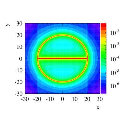
Figure 1: The target function $f(x,y)$ with linear (left) and logarithmic (right) $z$-scale.

The mapping function $g(x,y)$ can be split into two channels, a circular part $g_{\_}{1}(x,y)$ and a line segment $g_{\_}{2}(x,y)$.

The circular part can best be parameterized in polar coordinates with radius $r\in\mathbb{R}^{+}$ and polar angle $\phi\in[-\pi,\pi]$. The transformation from Cartesian to polar coordinates is denoted $\Phi:(x,y)\mapsto(r,\phi)=(\sqrt{x^{2}+y^{2}},\mathrm{atan}(y/x))$, and the modulus of the corresponding Jacobi determinant is $|J_{\_}{\Phi}|=r$. Random numbers are generated according to

$$\tilde{g}(r,\phi)=\frac{1}{2\pi^{2}}\frac{\Delta r}{(r-r_{\_}{0})^{2}+(\Delta r)^{2}}\,,$$ (16)

i.e. a truncated Cauchy distribution in $r$ in the interval $[0,\infty]$ centred around $r_{\_}{0}$ with a width parameter of $\Delta r$, and a uniform distribution in $\phi$ in the interval $[-\pi,\pi]$. The transformation into Cartesian coordinates is obtained via

$$g_{\_}{1}(x,y)=\tilde{g}_{\_}{1}(\Phi(x,y))\frac{1}{|J_{\_}{\Phi}|}\,.$$ (17)

The line segment is parameterized in Cartesian coordinates. Random numbers are generated according to a uniform distribution in $x$ in the interval $[-r_{\_}{0},r_{\_}{0}]$, and a Cauchy distribution in $y$ centred around $y_{\_}{0}=0$ with a width parameter of $\Delta r$. The parametrization of the second channel is thus

$$g_{\_}{2}(x,y)=\frac{1}{2\pi r_{\_}{0}}\frac{\Delta r}{(y-y_{\_}0)^{2}+(\Delta r)^{2}}\theta(r_{\_}{0}-|x|)\,.$$ (18)

We study two cases in the following. In the first one, the mapping function consists of the two contributions defined above, i.e. $g(x,y)=\frac{1}{2}g_{\_}{1}(x,y)+\frac{1}{2}g_{\_}{2}(x,y)$. This overall mapping function is identical to the target function, i.e. $g(x,y)\propto f(x,y)$, up to a global scaling factor, thus the prior knowledge of the target function is complete. In the second case, only the circular part is considered in the mapping function, i.e. $g(x,y)=g_{\_}{1}(x,y)$. The model misses a resonant feature and the prior knowledge of the target function is thus incomplete. We compare the measures defined for both cases using IS and the proposed $\mathrm{(MC)}^{3}$ algorithm based on 20 runs of five chains with 5M samples each. This is done for different values of $\beta$, in particular $[0,0.01,0.1,0.25,0.5,0.75,0.9,0.99,1.0]$, and the lag, $[1,2,5,10,20]$. The sampling efficiency for a pure MH transition kernel, i.e. $\beta=0$, is adjusted to 30% during the pre-run.

3.1.1 Sampling efficiency

Figure 2 shows the sampling efficiency for the $\mathrm{(MC)}^{3}$ algorithm as a function of $\beta$. Since the transition kernel is a linear combination of two kernels, the efficiency increases linearly from 30% at $\beta=0$ to $100$% ($50$%) at $\beta=1$ for the case of complete (incomplete) prior knowledge. In comparison, the sampling efficiencies for pure IS are $100$% and $0.01$%, respectively. Consequently, a pure IS with incomplete knowledge leads to factors of up to $5,000$ more calls to the target function compared to the $\mathrm{(MC)}^{3}$ algorithm.

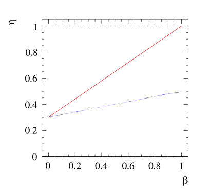
Figure 2: The sampling efficiency as a function of $\beta$ for the $\mathrm{(MC)}^{3}$ algorithm for complete (solid red) and incomplete prior knowledge (dotted blue). The 100% sampling efficiency for the IS algorithm is indicated as a dashed line.

3.1.2 Autocorrelation

As an example, the autocorrelation for $x$ is shown in Figure 3 for the case of complete (left) and incomplete knowledge (right). For the former case, the autocorrelation for $\beta=1$ is zero for all lags. This is expected since the function $f/g$ sampled from is uniform. For admixtures of the MH transition kernel, the autocorrelation increases to values of 95% or larger for $\beta=0$ and lags between 1 and 20. This large autocorrelation is owed to the small width of the proposal function used in the MH transition kernel in comparison with the size of $r_{\_}{0}$. As expected, the autocorrelation decreases with an increasing lag. A similar behaviour is observed for the case of incomplete knowledge with the exception that the autocorrelation does not reach zero but a plateau of around 35%.

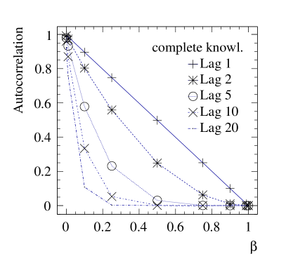
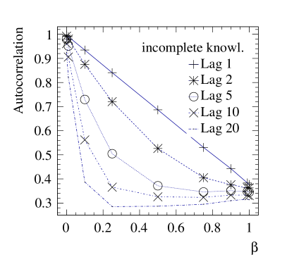
Figure 3: Autocorrelation for $x$ as a function of $\beta$ for the case of complete (left) and incomplete knowledge (right) and for different lags.

3.1.3 Sequence length

The sequence lengths for the cases of complete and incomplete prior knowledge and $\beta=1$ are shown in Figure 4 for a lag of one and $\beta=1$. As expected from the low autocorrelation, the typical sequence length in the case of complete prior knowledge is greater than one in less than a per mil of all cases. In contrast, sequences in the case of incomplete prior knowledge can reach lengths of greater than 1,000, although the most likely length is also one.

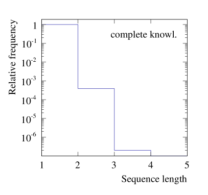
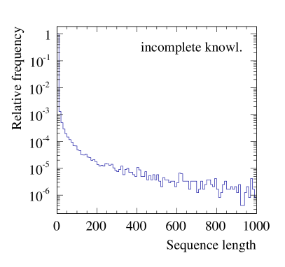
Figure 4: Sequence lengths for the cases of complete (left) and incomplete prior knowledge (right) for a lag of one and $\beta=1$.

Figure 5 shows the fraction of sequence lengths above 10 and 50 for the cases of complete and incomplete prior knowledge. As expected, these fractions drop in the former case with increasing beta and increasing lag. Both trends can be explained by the autocorrelation of the MH transition kernel. The fractions are typically smaller than in the case of incomplete knowledge for which the fractions increase with increasing beta and decrease with increasing lag. The former trend is due to the fact that the Markov Chains get stuck more often if the admixture of incomplete prior knowledge increases.

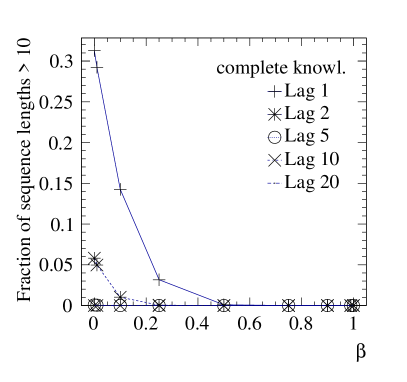
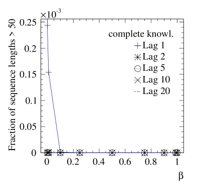
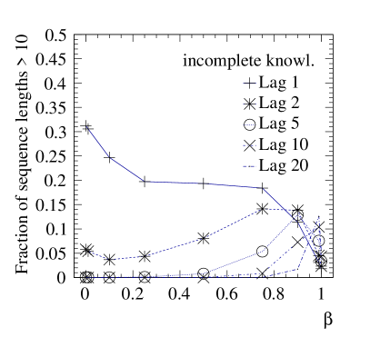
Figure 5: The fraction of sequence lengths greater than 10 (left) and 50 (right), for the case of complete knowledge (top) and incomplete knowledge (bottom), shown for lags between 1 and 20.

3.1.4 Convergence

As a test for the convergence of the Markov Chain, the phase space is divided in Cartesian coordinates into $50\times 50$ bins in a region $[-30,30]$ in $x$ and $y$. The distribution of the $\chi^{2}$ defined in Equation 14 is obtained by scaling the target function to the predefined number of samples, $N$, and by generating ensembles of two-dimensional histograms for which each bin is a random number drawn from a Poisson distribution around the expectation value of the scaled target function. The distribution of the $\chi^{2}$ variable is shown in Figure 6. It has a mean value of 2,500 and is wider than the expected $\chi^{2}$-distribution due to non-Gaussian fluctuations in the low-probability region of the target function.

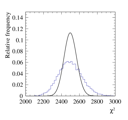
Figure 6: Observed (histogram) and expected $\chi^{2}$ distributions (solid line) calculated in the region $(x,y)\in[-30,30]^{2}$.

Figure 7 shows the mean of the $\chi^{2}$ distribution obtained from 100 runs of the $\mathrm{(MC)}^{3}$ algorithm as a function of $\beta$ for different lags. In the case of complete prior knowledge and a lag of one, the $\chi^{2}$ drops from roughly $15,000$ at $\beta=0$ to about $2,500$ at $\beta=1$. The behaviour for small values of $\beta$ is expected due to a large amount of autocorrelation between the samples if the MH transition kernel dominates. For large values of $\beta$ it is expected that a perfect prior knowledge leads to a fast convergence of the Markov Chain. The trend is similar for larger values of the lag where the mean $\chi^{2}$ converges to a constant value of about $2,500$ rather quickly.

In the case of incomplete knowledge the mean $\chi^{2}$ value is larger for $\beta=1$ compared to $\beta=0$, and the curve shows a minimum for a mixed transition kernel. The large $\chi^{2}$ values around $\beta=1$ can be explained by the fact that the proposal function does not sample the line segment of the target function homogeneously. The occurrence of a minimum in the curve shows that the sampling improves compared to a pure Metropolis–Hastings algorithm if prior knowledge is used, and that it cures the problem of incomplete knowledge for a pure IS algorithm. The minimal $\chi^{2}$ converges to $2,500$ with increasing lag.

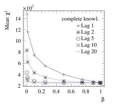
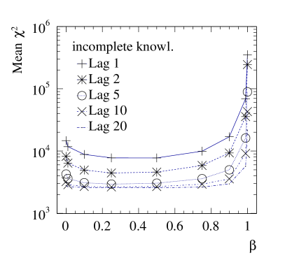
Figure 7: The mean $\chi^{2}$ as a function of $\beta$ for different lags for the case of complete (left) and incomplete prior knowledge (right).

3.2 Example two: a toy generator for Drell-Yan events

The second example represents an application of the $\mathrm{(MC)}^{3}$ algorithm we aim for in the future, namely the generation of unweighted events. The process under study is Drell-Yan production of lepton pairs in proton-proton collisions at an assumed centre-of-mass energy of 8 TeV. The target function is defined by the differential cross section in the partonic invariant mass squared of the lepton pair, $s$, the rapidity of the lepton system, $Y$, the scattering angle of the centre-of-mass system, $\theta$, and the azimuthal angle, $\phi$. The flavour of the incoming quark is fixed to the up-quark and the phase space is constrained to $\sqrt{s}\in[15,200]$ GeV, $Y\in[-6,6]$, $\cos{\theta}\in[-1,1]$ and $\phi\in[0,2\pi]$.

The mapping function is a sum of two mappings, namely the photon and $Z$-boson contributions, providing a reasonable approximation of the differential cross section. The remaining differences between the mapping function and the target function are small and caused by the interference of the two processes. Both mappings are uniform in $\phi$, sample from an optimized histogram in $Y$, and both encode the information about $\theta$ using a functional form of $1+\cos(\theta)^{2}$. The mapping function of the photon contribution follows $1/s^{2}$ while that of the $Z$-boson exchange is parametrized by a Breit–Wigner distribution characterized by the mass and decay width of the $Z$-boson. The channel weights are chosen as $\alpha_{\_}{\gamma}=0.76$ and $\alpha_{\_}{Z}=0.24$.

3.2.1 Characteristic numbers for the performance

Figure 8 (left) shows the sampling efficiency for the $\mathrm{(MC)}^{3}$ algorithm as a function of $\beta$. The efficiency increases linearly from 25% at $\beta=0$ to about 70% at $\beta=1$. In comparison, the sampling efficiency for the IS algorithm is about 55%.

An opposite trend can be observed for the autocorrelation in the same figure (right). It becomes smaller with increasing $\beta$ similar to the behaviour in the first example. The autocorrelation ranges from values of about 95% at $\beta=0$ to roughly 25% at $\beta=1$ for a lag of one. For larger values of the lag, the autocorrelation drops exponentially and vanishes at $\beta=1$ for lags greater than five. This observation is consistent with the fraction of sequence lengths greater than 10 and 50 as a function of $\beta$ which is shown in Figure 9. Both fractions decrease with increasing values of $\beta$ and for large lags.

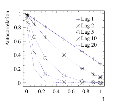
Figure 8: Left: The sampling efficiency as a function of $\beta$ for the $\mathrm{(MC)}^{3}$ algorithm. The sampling efficiency for the IS algorithm is indicated as a dashed line. Right: Autocorrelation for $\sqrt{s}$ as a function of $\beta$ for different lags.

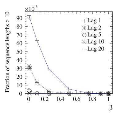
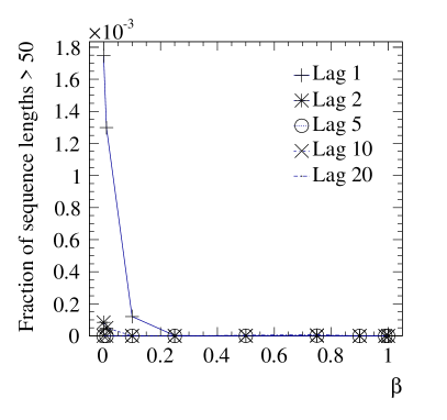
Figure 9: The fraction of sequence lengths greater than 10 (left) and 50 (right) shown for lags between 1 and 20.

The convergence of the Markov Chains is tested with a $\chi^{2}$ in the $\sqrt{s}$-variable. It is shown as a function of $\beta$ for different lags in Figure 10. The mean $\chi^{2}$ drops exponentially for increasing values of $\beta$. It decreases faster for an increasing choice of lag due to the reduced autocorrelation, and converges to the expected value of $100$.

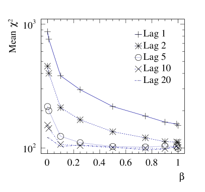
Figure 10: The mean $\chi^{2}$ as a function of $\beta$ for different lags.

When considering lags larger than one in this simple example, the overall efficiency of pure Multi-Channel Importance Sampling is still higher than that of $\mathrm{(MC)}^{3}$. However, in more complicated scenarios, e.g. for multi-particle final states with non-trivial phase-space cuts, one is typically confronted with unweighting efficiencies of the order of one percent or smaller when using Importance Sampling Monte Carlo, and we foresee a huge potential to improve these cases with our new algorithm.

3.3 Example three: $Z$ plus multijet production within SHERPA ​​

The third example extends upon the former one, aiming for a validation of the proposed method for a realistic and high-dimensional problem. We study the production of $Z$ bosons associated with $n$ additional jets at the LHC with a centre-of-mass energy of $\sqrt{s}=8\,\textup{TeV}$, and $n\in\{0,1,2,3,4\}$. We consider unweighted event generation according to the corresponding multi-parton tree-level matrix elements. The $Z$ boson is required to decay into a charged lepton pair and we constrain ourselves to diagrams involving exactly one electroweak propagator only. For this study we have implemented the $\mathrm{(MC)}^{3}$ algorithm within the SHERPA ​​event generator framework. The channels and mappings for the importance sampling kernel are obtained from the Multi-Channel Importance Sampler of SHERPA ​​, more specifically the AMEGIC generator [3]. Local variations of the phase-space points steered by the MH kernel are generated using the BAT framework [42]. For that the kinematic phase-space configuration of the outgoing particles of the $2\rightarrow N$ scattering process is mapped on $3N-4$ random variables with a parametrisation similar to the one presented in Ref. [44]. Technical details will be provided in a future publication.

To avoid physical singularities in the processes under consideration we need to regulate contributions from massless photon exchange and soft- and collinear QCD emissions. This is achieved by applying the following set of standard cuts:

• transverse momentum of the charged leptons $p_{\_}{T,\ell}\geq 20\,\textup{GeV}$;

• invariant mass of the lepton pair $66\,\textup{GeV}\leq m_{\_}{\ell\ell}\leq 116\,\textup{GeV}$;

• exactly $n$ anti-$k_{\_}T$ jets with transverse momenta $p_{\_}{T,j}\geq 30\,\textup{GeV}$ and distance parameter $R=0.4$.

During an initial prerun the channel weights of the importance sampling kernel are optimized such that the variance of the integral estimate, here the total cross section, is reduced. Then, for a kernel mixing parameter of $\beta=0.1$, the proposal width for each of the $3N-4$ parameters is adapted separately to yield a sampling efficiency between $0.35$ and $0.55$, respectively.

For each jet multiplicity we generated samples of unweighted events using both SHERPA ​​’s standard IS algorithm and the new $\mathrm{(MC)}^{3}$ sampler for a kernel mixing parameter of $\beta=0.8$. Table 1 compares the respective sampling efficiencies as a function of jet multiplicity $n$, based on a lag of 1 for the latter. For the original importance sampling approach used in SHERPA ​​the sampling efficiency decreases significantly with an increasing number of final-state jets.

$n$ jets	0	1	2	3	4
IS	$0.20$	$6.8\cdot 10^{-3}$	$3.1\cdot 10^{-3}$	$4.0\cdot 10^{-4}$	$2.9\cdot 10^{-6}$
$\mathrm{(MC)}^{3}$ $\beta=0.8$	$0.50$	$0.28$	$0.25$	$0.19$	$0.11$

Table 1: Sampling efficiency for $Z+n$ jets event generation with the $\mathrm{(MC)}^{3}$ algorithm as implemented in SHERPA ​​in comparison to pure Multi-Channel Importance Sampling (IS). A lag of 1 is used and the kernel mixing parameter is fixed to $\beta=0.8$.

With increasing final-state multiplicity the number of sub-processes as well as the number of Feynman diagrams, i.e. phase-space topologies and corresponding integration channels, per sub-process increases rapidly. This results in the significant drop of sampling efficiency for the original pure Multi-Channel Importance Sampler. Furthermore, with increasing jet multiplicity the computational costs for the evaluation of the matrix element per phase-space point rise rapidly.

In Table 2 the scaling behaviour of the sampling efficiency as a function of the kernel mixing parameter $\beta$ is presented for the process $Z+3$ jets. The expected linear decrease of $\eta$ with increasing values of $\beta$ is confirmed.

$\beta$	0.6	0.7	0.8	0.9
$\eta$	0.26	0.23	0.19	0.16

Table 2: Sampling efficiency $\eta$ for $Z+3$ jets production for the $\mathrm{(MC)}^{3}$ implementation in SHERPA ​​for different values of the mixing parameter $\beta$ using a fixed lag of 1.

Seemingly the $\mathrm{(MC)}^{3}$ approach outperforms pure Multi-Channel Importance Sampling by several orders of magnitude, in particular for high jet multiplicities. However, these improved sampling efficiencies have to be corrected by a lag in order to account for autocorrelation effects in the generated samples introduced by the design of the $\mathrm{(MC)}^{3}$ algorithm.

For the analysis of the statistical properties of the samples generated with $\mathrm{(MC)}^{3}$ we consider the case of $Z+3$ jets production. To reduce the autocorrelation in the $\mathrm{(MC)}^{3}$ samples an initial lag of 20 is applied during event generation. Introducing a lag in $\mathrm{(MC)}^{3}$, the remaining sequence lengths in the generated samples decrease. Figure 11 illustrates that the fractions of larger sequence lengths in the samples decrease indeed exponentially. With the initial lag of 20 during production, no sequence length above 15 is observed for any of the considered choices for $\beta$ and considering a sample of size 1M events. This simple measure of the autocorrelation increases with an increasing mixing parameter $\beta$. Note that the efficiencies quoted earlier have to be corrected for the lag. For the chosen working point, they still show a significant improvement over those obtained from a pure IS algorithm for large jet multiplicities.

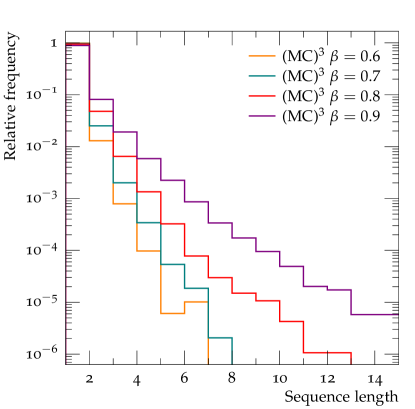
Figure 11: Sequence lengths distribution in $Z+3$ jets production using the $\mathrm{(MC)}^{3}$ algorithm with different values of the kernel mixing parameter $\beta$.

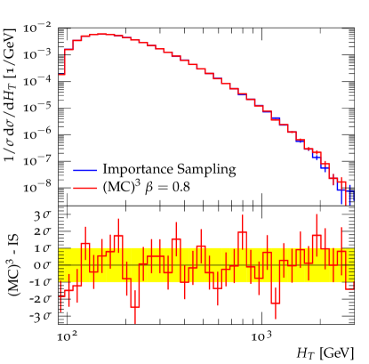
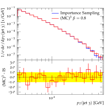
Figure 12: Normalized differential distributions for the third-jet transverse momentum $p_{\_}T$ (right) and the scalar sum of all jet transverse momenta $H_{\_}T$ (left) in $Z+3$ jets production. Shown are the predictions from pure Multi-Channel Importance Sampling (blue) and the $\mathrm{(MC)}^{3}$ algorithm with a lag of 20 and $\beta=0.8$. The lower panels indicate the statistical compatibility of the samples, measured in terms of standard deviations of the IS result.

We close our discussion of this example by testing the consistency of observable distributions predicted by the two algorithms for the $Z+3$ jets process. In Figure 12 we analyse the statistical compatibility of the sample generated with $\mathrm{(MC)}^{3}$ using a lag of 20 and a kernel mixing parameter $\beta=0.8$ with the reference sample generated using the original Multi-Channel Importance Sampling approach. We present results for the transverse momentum of the third jet, $p_{\_}T({\rm jet}\,3)$, and the scalar sum of all jet transverse momenta, $H_{\_}T$. As a measure for the statistical compatibility of the two samples we indicate in the lower panels the bin-wise difference measured in terms of standard deviations of the IS result. Clearly both approaches yield fully compatible results, not only for the observables presented here, allowing us to conclude that the $\mathrm{(MC)}^{3}$ algorithm yields a fully consistent event generation routine that can clearly supersede standard importance sampling methods in particular for high-multiplicity final states.

4 Conclusions

We have presented a new algorithm for phase-space sampling called $\mathrm{(MC)}^{3}$. It improves pure Markov Chain Monte Carlo techniques by incorporating prior knowledge about the target function from a corresponding Multi-Channel Importance Sampling algorithm. $\mathrm{(MC)}^{3}$ makes use of a linearly mixed transition kernel given by a locally acting Metropolis–Hastings component and an importance sampling kernel that allows for global jumps in phase space.

We have assessed the systematics of the new algorithm with three illustrative examples, thereby focusing on the sampling probability, autocorrelation effects and the convergence of the resulting Markov Chain. We have shown that incomplete prior knowledge can cause a severe drop in sampling efficiency when using Multi-Channel Importance Sampling, and thus an increased number of calls to the target function. Even for problems with a low number of dimensions, this can be particularly severe if resonant structures in the mapping function $g$ are missing. In contrast, the $\mathrm{(MC)}^{3}$ algorithm can increase the sampling efficiency because of the self-adapting properties of the produced Markov Chains. However, the resulting samples show an autocorrelation, and its strength depends on the amount of prior knowledge. The latter is controlled by the parameter $\beta$ and the lag. The impact of the autocorrelation can also be seen in the distribution of the sequence lengths and discrepancy variables which show differences between the true and the sampled distribution. A large autocorrelation also indicates a poor convergence of the Markov Chain to its limiting distribution. The autocorrelation can be suppressed to a reasonable level by choosing a small to moderate lag.

We have shown that the $\mathrm{(MC)}^{3}$ algorithm works very well for a low number of dimensions and that it performs better than the traditional Multi-Channel Importance Sampling for the case of incomplete prior knowledge. The third example also shows that the new algorithm outperforms the Importance Sampling algorithm for an increasing number of final-state particles when applied to the concrete task of producing unweighted events with Monte Carlo event generators.

References

- [1] A. Buckley, et al., General-purpose event generators for LHC physics, Phys. Rept. 504 (2011) 145.
- [2] F. Caravaglios, et al., A New approach to multijet calculations in hadron collisions, Nucl. Phys. B539 (1999) 215.
- [3] F. Krauss, R. Kuhn, G. Soff, AMEGIC++ 1.0: A Matrix element generator in C++, JHEP 0202 (2002) 044.
- [4] A. Cafarella, C. G. Papadopoulos, M. Worek, Helac-Phegas: A Generator for all parton level processes, Comput. Phys. Commun. 180 (2009) 1941.
- [5] W. Kilian, T. Ohl, J. Reuter, WHIZARD: Simulating Multi-Particle Processes at LHC and ILC, Eur. Phys. J. C71 (2011) 1742.
- [6] T. Gleisberg, S. Höche, Comix, a new matrix element generator, JHEP 0812 (2008) 039.
- [7] J. Alwall, et al., MadGraph 5 : Going Beyond, JHEP 1106 (2011) 128.
- [8] C. Berger, et al., An Automated Implementation of On-Shell Methods for One-Loop Amplitudes, Phys. Rev. D78 (2008) 036003.
- [9] A. van Hameren, C. Papadopoulos, R. Pittau, Automated one-loop calculations: A Proof of concept, JHEP 0909 (2009) 106.
- [10] V. Hirschi, et al., Automation of one-loop QCD corrections, JHEP 1105 (2011) 044.
- [11] G. Cullen, et al., Automated One-Loop Calculations with GoSam, Eur. Phys. J. C72 (2012) 1889.
- [12] F. Cascioli, P. Maierhofer, S. Pozzorini, Scattering Amplitudes with Open Loops, Phys. Rev. Lett. 108 (2012) 111601.
- [13] S. Badger, et al., Numerical evaluation of virtual corrections to multi-jet production in massless QCD, Comput. Phys. Commun. 184 (2013) 1981.
- [14] S. Actis, et al., Recursive generation of one-loop amplitudes in the Standard Model, JHEP 1304 (2013) 037.
- [15] G. Bevilacqua, et al., HELAC-NLO, Comput. Phys. Commun. 184 (2013) 986.
- [16] T. Gleisberg, et al., SHERPA 1. alpha: A Proof of concept version, JHEP 0402 (2004) 056.
- [17] T. Gleisberg, et al., Event generation with SHERPA 1.1, JHEP 0902 (2009) 007.
- [18] C. G. Papadopoulos, PHEGAS: A Phase space generator for automatic cross-section computation, Comput. Phys. Commun. 137 (2001) 247.
- [19] F. Maltoni, T. Stelzer, MadEvent: Automatic event generation with MadGraph, JHEP 0302 (2003) 027.
- [20] A. van Hameren, Kaleu: A General-Purpose Parton-Level Phase Space Generator, arXiv:1003.4953.
- [21] G. P. Lepage, A New Algorithm for Adaptive Multidimensional Integration, J. Comput. Phys. 27 (1978) 192.
- [22] T. Ohl, Vegas revisited: Adaptive Monte Carlo integration beyond factorization, Comput. Phys. Commun. 120 (1999) 13.
- [23] S. Jadach, Foam: Multidimensional general purpose Monte Carlo generator with selfadapting symplectic grid, Comput. Phys. Commun. 130 (2000) 244.
- [24] T. Hahn, CUBA: A Library for multidimensional numerical integration, Comput. Phys. Commun. 168 (2005) 78.
- [25] A. van Hameren, PARNI for importance sampling and density estimation, Acta Phys. Polon. B40 (2009) 259.
- [26] S. Brooks, et al., Handbook of Markov Chain Monte Carlo, Chapman and Hall/CRC, 2011.
- [27] H. Kharraziha, S. Moretti, The Metropolis algorithm for on-shell four momentum phase space, Comput. Phys. Commun. 127 (2000) 242.
- [28] S. Weinzierl, A General algorithm to generate unweighted events for next-to-leading order calculations in electron positron annihilation, JHEP 0108 (2001) 028.
- [29] R. Lafaye, et al., Measuring Supersymmetry, Eur. Phys. J. C54 (2008) 617.
- [30] R. Lafaye, et al., Measuring the Higgs Sector, JHEP 0908 (2009) 009.
- [31] N. Metropolis, et al., Equation of state calculations by fast computing machines, J. Chem. Phys. 21 (1953) 1087.
- [32] W. Hastings, Monte Carlo Sampling Methods Using Markov Chains and Their Applications, Biometrika 57 (1970) 97.
- [33] J. Skilling, Nested sampling for general bayesian computation, Bayesian Anal. 1 (4) (2006) 833.
- [34] B. C. Allanach, C. G. Lester, Sampling using a ‘bank’ of clues, Comput. Phys. Commun. 179 (2008) 256.
- [35] O. Cappe, et al., Adaptive importance sampling in general mixture classes, Stat. Comp. 18 (2008) 447.
- [36] R. V. Craiua, J. Rosenthala, C. Yanga, Learn from thy neighbor: Parallel-chain and regional adaptive mcmc, J. Am. Statist. Assoc. 104 (488) (2009) 1454.
- [37] F. Beaujean, A. Caldwell, Initializing adaptive importance sampling with Markov chains, arXiv:1304.7808.
- [38] F. James, Monte Carlo Theory and Practice, Rept. Prog. Phys. 43 (1980) 1145.
- [39] S. Weinzierl, Introduction to Monte Carlo methods, arXiv:hep-ph/0006269.
- [40] J. von Neumann, Various techniques used in connection with random digits, in: A. Householder, G. Forsythe, H. Germond (Eds.), Monte Carlo Methods, Vol. 12 of National Bureau of Standards Applied Mathematics Series, 1951, p. 36.
- [41] R. Kleiss, R. Pittau, Weight optimization in multichannel Monte Carlo, Comput. Phys. Commun. 83 (1994) 141.
- [42] A. Caldwell, D. Kollar, K. Kröninger, BAT: The Bayesian Analysis Toolkit, Comput. Phys. Commun. 180 (2009) 2197.
- [43] A. Gelman, D. B. Rubin, Inference from Iterative Simulation Using Multiple Sequences, Statist. Sci. 7 (1992) 457.
- [44] S. Plätzer, RAMBO on diet, arXiv:1308.2922.