Daily Variations of the Geomagnetic Field in the Brazilian zone.

Abstract

The solar quiet daily variation (Sq) was investigated with respect to the longitudinal and seasonal variations at the Brazilian geomagnetic ground stations of Tatuoca (TTB), Vassouras (VSS ) and São Martinho da Serra (SMS). The data utilized was collected during the time interval from January to May 2010. We employed the continuous wavelet transforms and cross wavelet coherence to study the spectral content and correlations of the time series in the time-frequency domain. We identified possible phenomena of regional or global scope that could be affecting the magnetic response measured at TTB, VSS and SMS observatories. As a result some signatures of planetary waves and semidiurnal tides in the Sq variability were obtained.

${\dagger}$ phone:(55)(21)35049142, fax:(55)(21)25807081.

I Introduction

It is well know that the normal solar activity alters the currents system in the ionosphere. It produces two magnetic effects which are prominent in the equatorial and mid-latitude regions and stronger at local noontime. The first is called solar quiet daily variation (Sq) and the second is the equatorial electrojet (EEJ). The EEJ takes place in a narrow belt of $\pm 3^{\circ}$ centered over the dip magnetic equator and about $105\,km$ high, which , flows eastward during the local daytime. Its effects at the Earth’s surface range up to about $100\,nT$. The Sq current, on the other hand, has its centres near $30^{\circ}$ magnetic (dip) latitude in both hemispheres, flowing counterclockwise in the northern and clockwise in the southern hemisphere and its magnetic effects range up to about $40\,nT$ near the Earth’s surface Forbes ; Rastogi ; Onwumechili ; Price . The EEJ and the Sq Current System interact with another atmospheric, magnetosphere and solar phenomena, e.g. planetary waves, magnetic storms and solar flares, which characterize its hemispherical asymmetries and its local and seasonal responses ALi & Pancheva_Book . Numerous investigations on these interaction mechanisms have been done analyzing geomagnetic data obtained from ground stations as well as from satellite magnetometers. Despite of the amount of works carried out, this theme remains the subject of active research, e.g., Padatella ; Sahai . The reasons of this interest are the requirements of more precise knowledges on the local variation of the geomagnetic field for the development of more accurate mathematical models and some still unclear aspects on the interaction mechanisms between different ionospheric phenomena.

There are former studies of the Daily Variation and the Equatorial Electrojet in the Brazilian zone using magnetic data from ground stations. These studies have been carried out basically processing magnetic data collected in campaigns during the International Equatorial Electrojet Year (IEEY, $Sep.\,1991\,\,Mar.\,1993$ ). These researches have covered mainly the dip equator zone and have been focused in the study of the EEJ Rastogi_2010 ; Rastogi_2009 ; Rastogi_2007 .

In this work it is investigated the day to day variability of the solar quiet day variation in the Brazilian zone. We used data from the geomagnetic stations of Tatuoca (TTB), Vassouras (VSS) and São Martinho da Serra (SMS), which cover from the dip equator to the mid-latitudes zone. The processed data covers the time interval of the first five months of the year 2010. The aim of this research is to explore the potentiality of the present high resolution magnetic data generated in on ground magnetic observatories localized in the Brazilian sector to investigate local characteristics of these ionospheric phenomena and also to explore the advantages that, for this type of investigation, the spectral analysis in the time-frequency domain offers.

II Data set

We used the data collected during the first five months of 2010 at the Brazilian Geomagnetic Observatories of Tatuoca (TTB), Vassouras (VSS ) and São Martinho da Serra (SMS). These observatories comprise almost all the Brazilian zone from mid-latitudes to the dip-equator (see Figure 1). The data consists of a record of $Hx$, $Hy$ and $Hz$ components of the geomagnetic field with a resolution of one second, which was processed and smoothed using a moving average filter reducing the resolution to one hour, which is more appropriated for daily variation studies.

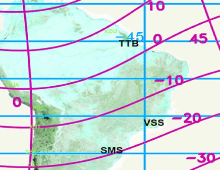
Figure 1: Map showing the locations of the relevant Brazilian observatories. Labels indicate the IAGA code of observatories. Geographic co-ordinates are: S. Martinho da Serra (-29,538, -53,855), Vassouras (-22,404, -43,663) and Tatuoca (-1,2001, -48,506).
Figure edited from $http://supermag.uib.no/info/img/SuperMAG_{E}arth_{G}EO.png$.

We have calculated the monthly means of the daily variation taking into account the international quietest days of the month, which are deduced from the planetary three-hour index Kp. The quietest days of the first ten months of the year 2010 are listed in Table 1. These data were obtained from the International Service of Geomagnetic Indices of the International Association of Geomagnetism and Aeronomy.

Table 1: International Quietest Days ($Q_{1}-Q_{10}$) for the year 2010. Data from GeoForschungsZentrum Potsdam, Adolf-Schmidt-Observatorium für Geomagnetismus, Germany

Quietest Days
Month      Year	$Q_{1}$	$Q_{2}$	$Q_{3}$	$Q_{4}$	$Q_{5}$	$Q_{6}$	$Q_{7}$	$Q_{8}$	$Q_{9}$	$Q_{1}0$
Jan.   2010	17	7	9	2	8	27	6	16	19	1
Feb.   2010	20	21	27	5	28	9	26	10	23	7
Mar.   2010	22	23	21	9	8	13	15	5	19	16
Apr.   2010	26	10	18	25	30	16	28	13	17	20
May   2010	23	24	27	9	13	15	1	14	22	16
Jun.   2010	12	20	8	19	9	23	14	11	22	7
Jul.   2010	10	17	18	7	13	6	19	8	5	16
Aug.   2010	30	22	21	29	14	20	31	13	19	7
Sep.   2010	11	12	30	4	22	10	3	13	19	20
Oct.   2010	2	1	4	1	3	30	21	7	28	10

III The Daily Variation

Here we are interested in the comparison of the local and seasonal response of the amplitude and phase of the daily variation (Sq) among the three geomagnetic observatories chosen for this study and to detect eventual occurrences of abnormal phases, i.e., when the maximum of Sq is reached out of the time interval [8:30-13:30]. For this purpose in this section we calculated the monthly means of the horizontal and vertical components for the five quietest days of each month. Former studies reveal the occurrences of abnormal variations of the phase and amplitude of the day to day variability of the Sq . In mid-latitudes the occurrence of these events has been attributed to northward and southward perturbation of the horizontal component of the geomagnetic field of large geographical extend and possible magnetospheric origin Butcher . On the other hand for the dip latitude this phenomenon has been attributed to the occurrence of partial equatorial counter-electrojet currents due to changes in local ionosphere dynamos. Other local factors could contribute to the regional variability of the solar quiet day variation, e.g., induction by the onshore horizontal component at the ocean-continent interface, oceans induction and conductivity anomalies Lilley .

The calculated monthly means of the quietest day variation are plotted in Figure 2. The data covers the period of Jan-May 2010. The left column shows the values of the horizontal component and the right column the vertical component. The rows indicate, from top to bottom, the ground stations of TTB, SMS and VSS. The curves show visible seasonal and latitudinal dependencies for the amplitude and phase of Sq. Here the phase is understand as the time at which the maximum amplitude of Sq is reached.

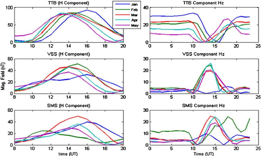
Figure 2: Monthly average of Sq at Tatuoca, Vassouras and S. Martinho da Serra.

In Figure 2 it can be observed an enhancement of the Sq signal at the Tatuoca station. This is a well known effect due to the equatorial electrojet phenomenon. It can be noted also that the horizontal component at TTB station shows its earliest phase and its minima amplitude in May and undergoes the maxima amplitude variability and latest phase in January. However, for VSS and SMS stations, the latest phase follows solely this behavior. At the same time it can be observed that the spread of the phase in VSS is larger than in TTB and smaller than in the SMS station. That is, the phase spread increases in the meridional direction. The vertical component in TTB follows a seasonal behavior similar to the horizontal one, but for VSS and SMS this component exhibits an abnormal lower amplitude variation in January. Former studies Butcher ; Hitchman have asserted that mid-latitude stations tend to have maximum Sq amplitudes (and advanced phase) at summer solstice, while at equatorial stations this tendency takes place at equinoctial times. In our case the results for VSS and SMS reveal that this maximum occurs for summer equinoxes and for the TTB observatory it is reached at the summer solstice.

Local asymmetries and atypical seasonal behavior of these ionospheric phenomena are expected to occur due to non-migrating tides and asymmetric tidal winds driven by the hemispheric asymmetries of the conductivity due to variations in the insolation particulary during the solstice season Padatella .

The bar plot of Figure 3 shows the daily range of Sq signal at the three stations for the first five months of 2010. In Figure 3 it can be observed a decreasing tendency of the Sq range at Tatuoca observatory, exhibiting its higher value at January, while for the other two stations it shows a bell shape with its maximum value in March. As can be expected this result confirms the same seasonal behavior shown in Figure 2. Comparing the values of the daily range in the Vasouras and S. Martinho da Serra it can be appreciated a monthly alternation of its maximum value. This seems to arise by coincidence because this parameter is sensitive to the Lloyds Seasons, i.e., to the equinoctial and solstice months, rather than to isolate months.

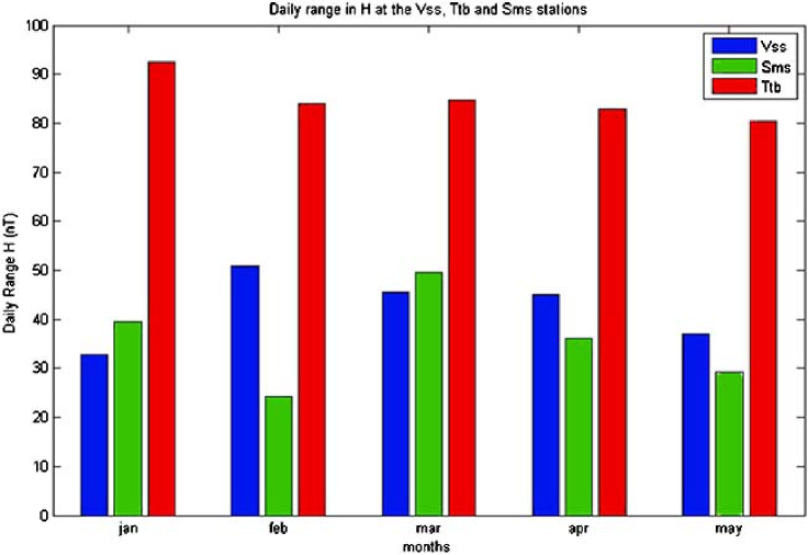
Figure 3: Comparison of the monthly means of the Daily Range at the stations of TTB, VSS and SMS from January to May of 2010.

Figure 4 shows two scatter plots for different stations pairs. The top panel shows a comparison of the daily variation at VSS station with respect to the other two. Here it can be seen that the better correlation is achieved for the station pair VSS/SMS with a correlation coefficient (CF) of 0.88, which falls for the station pair TTB/VSS to $CF=0.68$. This is an expected result due to their geographical locations. The bottom panel displays the comparison of this parameter at TTB related to VSS and SMS stations which are situated at a large distance with respect to the first one. Here it can be observed that in both cases the correlation is lower. This suggests that the seasonal response of the daily range at Tatuoca station, which is clearly different with respect to the other two, arises principally due to the additional contributions of the equatorial electrojet, which are absent at the other two stations. On the other hand the correlation of the daily range between Vassouras and S. Martinho da Serra is 0.88, which says that the bell shape of the seasonal response, showed by both stations, is due to the influence of the daily variation current and other local factors.

Figure 4: Comparison of the values of the Daily Range among the three stations from Jan-May 2010.

IV Wavelet Spectral Analysis

Wavelet spectral analysis allows us a quantitative monitoring of the signal evolution by decomposing a time-series into time-frequency space. In this way some problems associated to the Fourier method can be avoided, determining both the dominant modes of variability and how those modes vary in time. Wavelets are useful especially for signals that are non-stationary, have short-lived transient components, have features at different scales or have singularities Wavelet&Applications .

For the computation of the continuous wavelet transform (WT) we used a free script initially developed for oceanographic research torrence ; Torrence_Script . We use the Morlet wavelet to perform the spectral analysis. It is the better choice, when one is interested to look for special prints from other oscillatory phenomena, because this wavelet shows an acceptable localization in both time and frequency.

Figure 5 shows the calculated wavelet power spectrum of the horizontal component at Tatuoca. In this case the time series corresponds to the values measured during the month of January 2010. Here it can be observed a well defined peak corresponding to the daily variation during the whole month. In addition, it can be noted other two components corresponding to the semidiurnal period and to the 6-8 days period respectively. The semidiurnal signal arises in the form of wave trains around the 6th and 20th days. The 6-8 days period appears as an isolated peak, in the limit of the influence cone, also around the day 20. This day corresponds to one of the most disturbed days of the month.

In figures 5, 6 and 7 the wavelet spectral analysis for the signal at Tatuoca, Vassouras and S. Martinho da Serra stations for January 2010 are respectively presented. In all three stations, as should be expected, the component of the signal corresponding to the daily variation during all the month appears. The semidiurnal component at TTB station is visible during the first days of the month and around the 20th day, however at the others two stations the signal emerges only associated to the most disturbed day of the month. At the stations of VSS and SMS (Figures 6 and 7) components of the signal corresponding to the 2 days, 4 days and 6-8 days periods are visible. These oscillations arise also associated to the disturbed days. For the TTB station (Figure 5) only components for the 6-8 days periods are present.

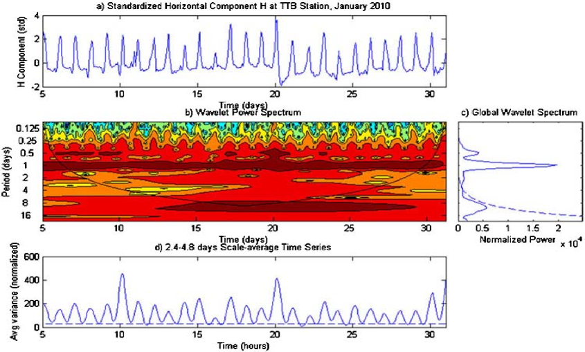
Figure 5: Wavelet Power Spectrum of the Magnetic Horizontal Component at Tatuoca Station for January 2010.

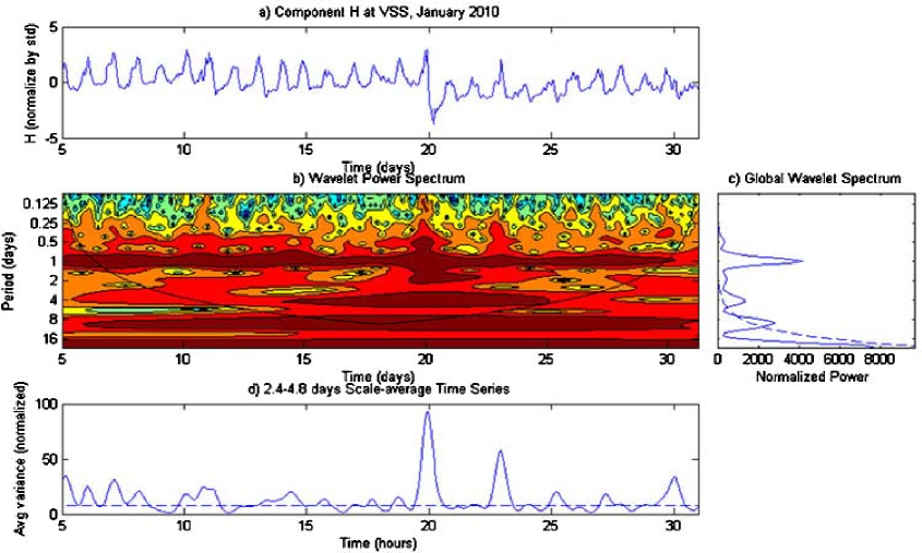
Figure 6: Wavelet Power Spectrum of the Magnetic Horizontal Component at Vassouras Station for January 2010.

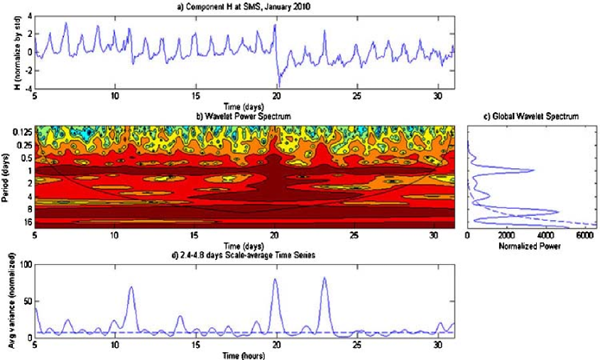
Figure 7: Wavelet Power Spectrum of the Magnetic Horizontal Component at S. Martinho da Serra Station for January 2010.

The Cross Wavelet Transform (XWT) and the wavelet coherence (WTC) have been used to analyze geophysical time series. Given two times series $x_{n}$ and $y_{n}$ and their respective continuous wavelet transforms $Wx$ and $Wy$ the XWT is defined as $W_{xy}\,=\,W_{x}\,W_{y}^{*}$. As the XWT is a complex magnitude it is useful to define the cross wavelet power as $|W_{xy}|^{2}$ and the phase difference as $arg(W_{xy})$, which can describe the common power and relative phase between $x_{n}$ and $y_{n}$ in time-frequency space. See Grinsted for details.

The concept of coherence between two time series appeared initially extending the definition of the cross correlation using notions of grade of coherence in classical optics Wiener . The Wavelet Coherence is a natural extension to the time-frequency domain of this former definition . It tells us how much coherent the Cross Wavelet Spectrum is, allowing us to seek confirmation of causal links between both time series.

We have analyzed two pairs of time series in order to test possible relationships between them. The first pair formed by the signals from VSS and SMS geomagnetic Stations and the second one formed by the signals from VSS and TTB stations. The power wavelet transform of each separated time series was examined above (see figures 5, 6 and 7) and there were detected some common characteristics that we will checkout with this method.

Figure 8 shows the standardized cross power spectrum (XWP) and the Wavelet Coherence of signals pairs for January 2010. It is also indicated the $5\%$ confidence level by a thick contour and the influence cone. In Figure 8 it can be noted, as expected, more significative zones of common power for the pair VSS-SMS than for the VSS-TTB one. The XWP of the pairs VSS-SMS and VSS-TTB are shown in the upper-right and upper-left panels respectively. In these two plots it can be appreciated that both pairs exhibit a significative common power, during all the month, for the period corresponding to the daily variation. For the semidiurnal period it is also observed a significant common cross power, but only for some time intervals. For the VSS-SMS pair it appears for the 5^th to 12^th days and around the 17^th to 21^th days. For the VSS-TTB pair this zone is extended to the last week of the month. For the XWP of the VSS-SMS pair, besides these significant zones of common power, other zones of common power centered around periods of $2$, $4$ and $8$ days also appear. For the VSS-TTB pair the common XWP in these zones appears weaker and only survives the zone around the period of $8$ days. However, as these zones are below the confidence level, we can only speculate about causal links between time series for those periods.

Figure 8: Cross Wavelet Power Spectrum (upper panel) and Wavelet Coherence for the pairs: VSS vs. TTB (right) and VSS vs. SMS (left), for Janurary 2010. The arrows indicate the relative phase. Is indicated also the cone of influence, with the thick contour designating the $5\%$ significance level.

Lower panels of Figure 8 display the wavelet transform coherence (WTC) of the signal pairs VSS-SMS (left) and VSS-TTB (right). In both panels it can be seen that the zone of higher coherence, above the confidence level, covers a greater area comparing with the corresponding area calculated for the Cross Wavelet Power Spectra (XWP). For example, the zone around the 2 and 8 days periods corresponding to the time interval from the 19^th to 25^th days now appears inside the confidence zone for both pairs. However for the zone around the 4 days period it appears included for the VSS-SMS pair, but not for the VSS-TTB one. It also appears more evident the coherence for the semidiurnal period that now includes also the last week for the VSS-SMS pair.

In Figure 8 an arrows mesh indicates the relative phase between time series. When the arrows point to the right indicate that both time series are in-phase and the first series leads the second one. Arrows pointing to left means that the series are in anti-phase and the first series lags the second one. For the VSS-SMS pair it can be observed that time series are in phase for all the periods, except for the time interval from the 5^th to the 13^th days, where in the zone of the semidiurnal period the time series at VSS station lags the corresponding one at SMS and for the zone of diurnal period, where the series at VSS leads the series at SMS. For the VSS-TTB pair it can be observed, for the diurnal period, that the time series at VSS station leads the corresponding one at TTB station during the first 12 days. Around the 15^th day, the series at VSS starts to follows the series at TTB and remains, for the rest of the month, following the series at TTB with a relative phase of $90^{\circ}$. For the zone comprising the periods from $4$ to $8$ days and the time interval from the 15^th to 20^th days, the series at VSS seems to lead the series at TTB with a small relative phase.

V Discussion

Employing the cross wavelet and wavelet coherence we detected common oscillations, with periods around the $2\,$, $4\,$ and $8\,$ days, in the horizontal magnetic component for the three magnetic observatories. Taking into account the geographic distances between these stations and its periods it can be inferred that such oscillations are due to planetary waves. In Figure 8 it can be observed that the oscillations around the $2\,d$, $4\,d$ and $8\,d$ periods appeared associated to the days 10^th to 21^st, which were the more perturbed days of the analyzed time interval. Oscillations of such periods, connected also to disturbed days, have been observed from meteor radar measurements of mesosphere and ionosphere of the Brazilian equatorial zone Takahashi and in the northwestern Pacific zone Yuji .

In Figure 8 the wavelet coherence spectrum shows Quasi-2d oscillations (QTDO), within the confidence zone, for the VSS-SMS pair. This result concords with the fact that in the Southern Hemisphere the occurrence of QTD stratospheric planetary waves has a maximum around January Plumb . However the VSS-TTB pair does not exhibit such oscillation, because the wavelet power spectrum of the signal at the TTB station (see Figure 5) does not hold significative spectral content at these periods. This is an unusual fact since QTDO are more frequent at the dip equator than at mid-Latitudes. QTDO have been reported in the equatorial electrojet (EEJ), with a peak at late solstice months (i.e., during January, February, July and August) Gurubaran . The fact that we have not found them at TTB could be explained by the fact that such oscillations in the EEJ are not always linked with planetary waves.

VI Summary and Conclusions

The daily variation was studied during the first five months of 2010 using the data form three geomagnetic observatories located in the Brazilian zone. Well known results were reproduced, e.g., the enhancement of Sq and the seasonal behavior of the daily range at the equatorial electrojet zone. However an anomalous oscillatory seasonal behavior was obtained for the daily range for the stations of VSS and SMS. The seasonal response obtained for the phase of maximum Sq amplitude also differs from former results.

Employing the wavelet analysis zones of significant spectral power for the periods of $1/2\,d$ and $1\,d$ which are related with the diurnal and semidiurnal tides were detected. There were also obtained contributions in the Sq response from oscillation around the $2\,d$, $4\,d$ and $8\,d$ periods, which can be interpreted as signatures of planetary waves on the Sq response. It should be noted that the spectral analysis was carried out using a relatively small data set. A future research must involve others geomagnetic observatories and larger time series in order to improve the characterization of the seasonal behavior of such oscillations in the geomagnetic data.

- (1) Forbes, J. (1981), The equatorial electrojet, Rev. Geophys., 19, 469- 504.
- (2) Rastogi, R. (1989), The equatorial electrojet, in Geomagnetism, vol. 3, edited by J. Jacobs, pp. 461- 525, Academic, San Diego, Calif.
- (3) Onwumechili, C. A. (1997), The Equatorial Electrojet, Gordon and Breach,Amsterdam, Netherlands.
- (4) Albert T. Price. Daily Variations of the Geomagnetic Field. Space Science Rewiews 9 (1969) 151-197.
- (5) M. Ali Abdu, D. Pancheva. Aeronomy of the Earth’s Atmosphere and Ionosphere. Springer, Feb 26, 2011 - Science - 501 pages.
- (6) N. M. Pedatella, et al. Seasonal and longitudinal variations of the solar quiet (Sq) current system during solar minimum determined by CHAMP satellite magnetic field observations. Journal of Geophysical Research: Space Physics, Volume 116, Issue A4, April 2011.
- (7) Y. Sahai, et al. Studies of ionospheric F-region response in the Latin American sector during the geomagnetic storm of 21 22 January 2005. Ann. Geophys., 29, 919-929, 2011.
- (8) R G Rastogi, et al. Equatorial electrojet in east Brazil longitudes. J. Earth Syst. Sci. 119, No. 4, August 2010, pp. 497 505
- (9) R. G. Rastogi and N. B. Trivedi. Asymmetries in the equatorial electrojet around N-E Brazil sector. Ann. Geophys., 27, 1233 1249, 2009.
- (10) R. G. Rastogi, et al. Day-to-day correlation of equatorial electrojet at two stations separated by 2000km. Ann. Geophys., 25, 875 880, 2007.
- (11) E. C. Butcher and G. M. Brown. On the nature of abnormal quiet days in Sq(H). Geophys. J. R. astr. Soc. (1981) 64,513-526
- (12) F. E. M. Lilley and R. L. Parker. Magnetic Daily Variations Compared Between the East and West Coasts of Australia. Geophys. J. R. astr. SOC. (1976) 44, 719-724.
- (13) A. P. Hitchman, et al. The quiet daily variation in the total magnetic field: global curves. Geophysical Research Letters, Vol. 25, NO. 11, pag. 2007-2010, 1998.
- (14) Wavelet Analysis and Applications.Qian Tao, Vai Mang I., Xu Yuesheng, Eds. Applied ans Numerical Harmonics Analysis, 3-11 2006 BirkHäuser Vrlag Basel /Switzerland
- (15) Available at URL: http://paos.colorado.edu/research/wavelets/.
- (16) Christopher Torrence and Peter J. Webster. The annual cycle of persistence in the El N o/Southern Oscillation. Journal of the Royal Meteorological Society, Volume 124, Issue 550, pages 1985 2004, July 1998 Part B
- (17) A. Grinsted, et al. Application of the cross wavelet transform and wavelet coherence to geophysical time series. Nonlinear Processes in Geophysics (2004) 11: 561 566 SRef-ID: 1607-7946/npg/2004-11-561.
- (18) Wiener N. Extrapolation, Interpolation, and Smoothing of Stationary Time Series: With Engineering Applications. MIT Press; 1949.
- (19) H. Takahashi, et al. Signatures of 3 6 day planetary waves in the equatorial mesosphere and ionosphere. Ann. Geophys., 24, 3343 3350, 2006
- (20) Yuji Yamada. 2-day, 3-day, and 5 6-day oscillations of the geomagnetic field detected by principal component analysis. Earth Planets Space, 54, 379 392, 2002.
- (21) R. Alan Plumb. On the seasonal cycle of stratospheric planetary waves. Pure and Applied Geophysics, Volume 130, Issue 2-3, pp 233-242, 1989
- (22) S. Gurubaran, et al. Signatures of quasi-2-day planetary waves in the equatorial electrojet: results from simultaneous observations of mesospheric winds and geomagnetic field variations at low latitudes. Journal of Atmospheric and Solar-Terrestrial Physics 63 (2001) 813 821