Modeling the wind circulation around mills with a Lagrangian stochastic approach

Mireille Bossy mireille.bossy@inria.fr Tosca Laboratory, Inria Sophia Antipolis – Méditerranée, France José Espina Inria, Chile Jacques Morice jacques.morice@inria.cl Inria, Chile Cristián Paris cristian.paris@inria.cl Inria, Chile Antoine Rousseau antoine.rousseau@inria.fr Lemon Laboratory, Inria Sophia Antipolis – Méditerranée, France
Abstract

This work aims at introducing model methodology and numerical studies related to a Lagrangian stochastic approach applied to the computation of the wind circulation around mills. We adapt the Lagrangian stochastic downscaling method that we have introduced in [3] and [4] to the atmospheric boundary layer and we introduce here a Lagrangian version of the actuator disc methods to take account of the mills. We present our numerical method and numerical experiments in the case of non rotating and rotating actuator disc models. First, for validation purpose we compare some numerical experiments against wind tunnel measurements. Second we perform some numerical experiments at the atmospheric scale and present some features of our numerical method, in particular the computation of the probability distribution of the wind in the wake zone, as a byproduct of the fluid particle model and the associated PDF method.

Key words: Lagrangian stochastic model; PDF method; atmospheric boundary layer; actuator disc model

1 Introduction

Modeling the flow through wind turbines and wind farms is a research area of growing importance with the fast and worldwide development of installed wind farms. Therefore there exists a wide variety of approaches that combine atmospheric computational fluid dynamics methods (CFD) with wake models (from actuator disc models to full rotor computations, see eg. Sørensen and Myken  [30], Hallanger and Sand [13], Bergmann and Iollo [2]).

Most popular atmospheric boundary layer computations are based on Reynolds averaged Navier-Stokes (RANS) turbulence models and large eddy simulation (LES) approaches. PDF methods, based on stochastic Lagrangian models, constitutes an interesting alternative (see the discussions in Pope [25]) that have been not yet fully developed in the case of atmospheric boundary layer modeling but are mostly used for reactive flows because this approach does not necessitate to approximate the reaction terms (Haworth [15], Minier and Peirano [21]). Among the reasons that can explain this phenomena, we can first rise the fact that such kinds of models handle nonlinear stochastic differential equations that necessitate a background on stochastic calculus, rather than classical PDE analysis. Second, the development of numerical solvers, based on stochastic particles approximation, requires the design of a hybrid Lagrangian/Eulerian algorithm from scratch. However, it is worth mentioning PDF methods are computationally inexpensive and allow to refine the space scale without any numerical constraints.

In recent works, some of the authors developed modeling numerical frameworks for the downscaling problem in meteorology (see [3],[4]). An algorithm called Stochastic Downscaling Method (SDM) is currently under validation when coupled with a coarse resolution wind prediction, provided thanks to classical numerical weather prediction (NWP) solvers. Quite a few widely used predictive numerical solvers (such as the weather research & forecasting model (WRF)) are based on a LES approach. To this purpose, we have developed a branch of SDM that includes atmospheric boundary layer modeling and ground interaction (log law).

In this paper, we present our methodology to introduce wake models (typically actuator disc models) in the SDM solver. We also present the related numerical experiments on wake computation, in a classical log law context.

We emphasize the fact that the basis of stochastic Lagrangian models consists in describing the stochastic dynamics of a fluid particle’s state variables (Xt,Ut)subscriptX𝑡subscriptU𝑡({\rm X}_{t},{\rm U}_{t}), under an appropriated probabilistic space (Ω,,)Ω(\Omega,{\mathcal{F}},{\mathbb{P}}) equipped with the expectation operator 𝔼𝔼\displaystyle{\mathbb{E}}. The Lagrangian approach allows to define the Eulerian average of the velocity, classically represented by the bracket operator Udelimited-⟨⟩U{{\displaystyle{\langle}{{\rm U}}\displaystyle{\rangle}}} in the RANS approach or U~~𝑈\widetilde{U} in the LES approach, as the mathematical conditional expectation111We consider here only the case of constant mass density, for the sake of clarity. In other cases a scalar state variable is introduced such as temperature, that weights the conditional expectation operator. of the particle velocity UtsubscriptU𝑡{\rm U}_{t} knowing its position x3xsuperscript3{\rm x}\in\mathbb{R}^{3}

U(t,x):=𝔼[Ut|Xt=x],assigndelimited-⟨⟩U𝑡x𝔼delimited-[]conditionalsubscriptU𝑡subscriptX𝑡x{{\displaystyle{\langle}{{\rm U}}\displaystyle{\rangle}}}(t,{\rm x}):=\displaystyle{\mathbb{E}}\left[{\rm U}_{t}|{\rm X}_{t}={\rm x}\right], (1.1)

and more generally, for any function f𝑓f,

f(U)(t,x):=𝔼[f(Ut)|Xt=x].assigndelimited-⟨⟩𝑓U𝑡x𝔼delimited-[]conditional𝑓subscriptU𝑡subscriptX𝑡x{{\displaystyle{\langle}{f({\rm U})}\displaystyle{\rangle}}}(t,{\rm x}):=\displaystyle{\mathbb{E}}\left[f({\rm U}_{t})|{\rm X}_{t}={\rm x}\right]. (1.2)

Equivalently, in term of PDF222Probability Density Function modeling approach (see [25] for further details) the Eulerian density at time t𝑡t and at a given x𝑥x is identified with the conditioned Lagrangian density, knowing the event {Xt=x}subscript𝑋𝑡𝑥\{X_{t}=x\}.

The connections between RANS/LES models and stochastic Lagrangian models are realized via a specific design of the stochastic equation coefficients for (Xt,Ut)subscriptX𝑡subscriptU𝑡({\rm X}_{t},{\rm U}_{t}) allowing to reproduce kε𝑘𝜀k-\varepsilon and Reynolds-stress models (see the review on Lagrangian modeling in Pope [24] and the discussion in [4]). In particular such PDF models can be used to reconstitute subgrid information of fluctuations in LES modeling.

After a short description of the SDM modeling, mathematical framework, and numerical method in Section 2, we introduce our Lagrangian version of the actuator disc modeling in Section 3. For validation purpose, in Section 4 we compare some numerical experiments against wind tunnel measurements. Section 5 is devoted to some numerical experiments at the atmospheric scale. To assess the mill impact in the flow, SDM simulations are run in both experiments with the two turbine models presented in Section 3, namely: the non-rotating actuator disc model, and the rotating actuator disc model.

2 Stochastic downscaling methodology

This section is devoted to the description of the Stochastic Downscaling Method, in the framework of turbulence modeling of an incompressible flow in the neutral case (constant mass density).

Consider the computational domain 𝒟𝒟\mathcal{D} as an open bounded subset of 3superscript3\mathbb{R}^{3}. In order to model the flow in 𝒟𝒟\mathcal{D}, we consider a couple of stochastic processes (Xt,Ut)subscriptX𝑡subscriptU𝑡({\rm X}_{t},{\rm U}_{t}) that respectively describe the location and the velocity of a generic fluid-particle. The evolution of (Xt,Ut)subscriptX𝑡subscriptU𝑡({\rm X}_{t},{\rm U}_{t}) is governed by the following generic system of stochastic differential equations (SDEs):

dXt=𝑑subscriptX𝑡absent\displaystyle d{\rm X}_{t}= Utdt,subscriptU𝑡𝑑𝑡\displaystyle{\rm U}_{t}dt, (2.1a)
dUt=𝑑subscriptU𝑡absent\displaystyle d{\rm U}_{t}= (1ϱx𝒫(t,Xt))dtG(t,Xt)(UtU(t,Xt))dt+C(t,Xt)dWt.1italic-ϱsubscriptx𝒫𝑡subscriptX𝑡𝑑𝑡𝐺𝑡subscriptX𝑡subscriptU𝑡delimited-⟨⟩U𝑡subscriptX𝑡𝑑𝑡𝐶𝑡subscriptX𝑡𝑑subscript𝑊𝑡\displaystyle\left(-\frac{1}{\varrho}\nabla_{{\rm x}}\langle{\mathscr{P}}\rangle(t,{\rm X}_{t})\right)dt-G(t,{\rm X}_{t})\Big{(}{\rm U}_{t}-\langle{\rm U}\rangle(t,{\rm X}_{t})\Big{)}dt+C(t,{\rm X}_{t})dW_{t}. (2.1b)

Here W𝑊W is a standard 3-dimensional Brownian motion, G𝐺G, C𝐶C and Uextsubscript𝑈ext{U_{\textrm{ext}}} are functions to be defined in accordance with the turbulence underlying model (see Section 2.3 below), and X(t=0)=X0𝑋𝑡0subscriptX0X(t=0)={\rm X}_{0}, U(t=0)=U0U𝑡0subscriptU0{\rm U}(t=0)={\rm U}_{0} where (X0,U0)subscriptX0subscriptU0({\rm X}_{0},{\rm U}_{0}) are random variables whose probability law μ0subscript𝜇0\mu_{0} is given. The parameter ϱitalic-ϱ\varrho is the mass density of the fluid (which is assumed to be constant).

We supplement the dynamics (2.1), with generic (Dirichlet) boundary conditions on the mean velocity:

U(t,x):=𝔼[Ut|Xt=x]=Uext(t,x),assigndelimited-⟨⟩U𝑡x𝔼delimited-[]conditionalsubscriptU𝑡subscriptX𝑡xsubscript𝑈ext𝑡x{{\displaystyle{\langle}{{\rm U}}\displaystyle{\rangle}}}(t,{\rm x}):=\displaystyle{\mathbb{E}}\left[{\rm U}_{t}|{\rm X}_{t}={\rm x}\right]={U_{\textrm{ext}}}(t,{\rm x}), (2.2)

when x=(x,y,z)x𝑥𝑦𝑧{\rm x}=(x,y,z) belongs to the lateral-boundary part or top-boundary part of 𝒟𝒟\partial\mathcal{D}. The bottom-boundary condition that should account for the surface roughness is described in Section 2.4.

2.1 Mathematical framewrok

According to (1.1), the term U(t,Xt)=𝔼[Ut|Xt]delimited-⟨⟩U𝑡subscriptX𝑡𝔼delimited-[]conditionalsubscriptU𝑡subscriptX𝑡{{\displaystyle{\langle}{{\rm U}}\displaystyle{\rangle}}}(t,{\rm X}_{t})=\displaystyle{\mathbb{E}}\left[{\rm U}_{t}|{\rm X}_{t}\right] denotes the expected velocity of the particle conditioned by its position XtsubscriptX𝑡{\rm X}_{t}, making the equation (2.1) a nonlinear SDEs in the sense of McKean. This means that a Markovian solution to (1.1) must be a process ((Xt,Ut); 0tT)subscript𝑋𝑡subscript𝑈𝑡 0𝑡𝑇((X_{t},U_{t});\,0\leq t\leq T) complemented with the set of its time-marginal laws ρ(t)𝜌𝑡\rho(t) of (Xt,Ut)subscript𝑋𝑡subscript𝑈𝑡(X_{t},U_{t}) at any time  0tT 0𝑡𝑇\,0\leq t\leq T, which allows to define (assuming the existence of densities for the marginal laws ρ(t)𝜌𝑡\rho(t))

𝔼[f(Ut)|Xt=x]𝔼delimited-[]conditional𝑓subscriptU𝑡subscriptX𝑡x\displaystyle{\mathbb{E}}\left[f({\rm U}_{t})|{\rm X}_{t}={\rm x}\right]

for any measurable function f𝑓f, as the conditional Lagrangian mean

3f(u)ρ(t,x,u)𝑑u3ρ(t,x,u)𝑑usubscriptsuperscript3𝑓𝑢𝜌𝑡𝑥𝑢differential-d𝑢subscriptsuperscript3𝜌𝑡𝑥𝑢differential-d𝑢\frac{\int_{\mathbb{R}^{3}}f(u)\rho(t,x,u)du}{\int_{\mathbb{R}^{3}}\rho(t,x,u)du}

whenever the marginal mas 3ρ(t,x,u)𝑑usubscriptsuperscript3𝜌𝑡𝑥𝑢differential-d𝑢\int_{\mathbb{R}^{3}}\rho(t,x,u)du is positive. In the framework of turbulent modeling this conditional Lagrangian mean is then identified to the Eulerian mean (see Pope [25] and the references therein)

In a series of papers, (see in particular Bossy and Jabir [6], Bossy, Jabin, Jabir and Fontbona [5], and references therein), the wellposedness of toy-models version of stochastic Lagrangian models, typically with drift coefficients of the velocity equation expressed as conditional expectation with respect to position, was initiated.

The wellposedness of the stochastic process ((Xt,Ut); 0tT)subscript𝑋𝑡subscript𝑈𝑡 0𝑡𝑇((X_{t},U_{t});\,0\leq t\leq T), for any arbitrary finite time T>0𝑇0T>0, whose time-evolution is given by the McKean-nonlinear SDE

{Xt=X0+0tUs𝑑s,Ut=U0+0tB[Xs;ρ(s)]𝑑s+σWt, where ρ(t) is the density law of (Xt,Ut) for all t(0,T],\left\{\begin{aligned} &X_{t}=X_{0}+\int_{0}^{t}U_{s}\,ds,\\ &U_{t}=U_{0}+\int_{0}^{t}B[X_{s};\rho(s)]ds+\sigma W_{t},\mbox{ where }\rho(t)\mbox{ is the density law of }(X_{t},U_{t})\mbox{ for all }t\in(0,T],\end{aligned}\right. (2.3)

can by found in [6], where W𝑊W is a standard dsuperscript𝑑\mathbb{R}^{d}-Brownian motion, the diffusion σ𝜎\sigma is a positive constant, and the drift coefficient (x,ψ)B(x,ψ)maps-to𝑥𝜓𝐵𝑥𝜓(x,\psi)\mapsto B(x,\psi) is the mapping from 𝒟×L1(𝒟×d)𝒟superscript𝐿1𝒟superscript𝑑\mathcal{D}\times L^{1}(\mathcal{D}\times\mathbb{R}^{d}) to dsuperscript𝑑\mathbb{R}^{d} defined by

B[x;ψ]=db(v)ψ(t,x,v)𝑑vdψ(t,x,v)𝑑v𝟙{dψ(t,x,v)𝑑v0}𝐵𝑥𝜓subscriptsuperscript𝑑𝑏𝑣𝜓𝑡𝑥𝑣differential-d𝑣subscriptsuperscript𝑑𝜓𝑡𝑥𝑣differential-d𝑣subscript1subscriptsuperscript𝑑𝜓𝑡𝑥𝑣differential-d𝑣0B[x;\psi]=\dfrac{\int_{\mathbb{R}^{d}}b(v)\psi(t,x,v)dv}{\int_{\mathbb{R}^{d}}\psi(t,x,v)dv}{\mathds{1}}_{\{\int_{\mathbb{R}^{d}}\psi(t,x,v)dv\neq 0\}} (2.4)

where b:dd:𝑏superscript𝑑superscript𝑑b:\mathbb{R}^{d}\rightarrow\mathbb{R}^{d} is a given bounded measurable function. This definition of the drift B𝐵B makes the mapping (t,x)B[x;ρ(t)]maps-to𝑡𝑥𝐵𝑥𝜌𝑡(t,x)\mapsto B[x;\rho(t)] coincides with (t,x)𝔼[b(Ut)|Xt=x]maps-to𝑡𝑥𝔼delimited-[]conditional𝑏subscript𝑈𝑡subscript𝑋𝑡𝑥(t,x)\mapsto\displaystyle{\mathbb{E}}[b(U_{t})|X_{t}=x] and the velocity equation rewrites

Ut=U0+0t𝔼[b(Us)|Xs]𝑑s+σWtsubscript𝑈𝑡subscript𝑈0superscriptsubscript0𝑡𝔼delimited-[]conditional𝑏subscript𝑈𝑠subscript𝑋𝑠differential-d𝑠𝜎subscript𝑊𝑡U_{t}=U_{0}+\int_{0}^{t}\displaystyle{\mathbb{E}}[b(U_{s})|X_{s}]ds+\sigma W_{t}

or equivalently, using the notation in (1.1)

dUt=b(U)(t,Xt)dt+σdWt.𝑑subscript𝑈𝑡delimited-⟨⟩𝑏𝑈𝑡subscript𝑋𝑡𝑑𝑡𝜎𝑑subscript𝑊𝑡dU_{t}={{\displaystyle{\langle}{b(U)}\displaystyle{\rangle}}}(t,X_{t})dt+\sigma dW_{t}.

Moreover a particle system, based on kernel regression estimator of the conditional expectation B𝐵B is shown to converge weakly to the model (2.3). The construction of the particle approximation is based on local averaging estimate on a N𝑁N-particle set (Xti,Uti,i=1,,N,t[0,T])formulae-sequencesubscriptsuperscript𝑋𝑖𝑡subscriptsuperscript𝑈𝑖𝑡𝑖1𝑁𝑡0𝑇(X^{i}_{t},U^{i}_{t},i=1,\ldots,N,t\in[0,T]) of

𝔼[b(Ut)|Xt=x] by i=1N𝒲N,i(x)b(Uti).𝔼delimited-[]conditional𝑏subscript𝑈𝑡subscript𝑋𝑡𝑥 by superscriptsubscript𝑖1𝑁subscript𝒲𝑁𝑖𝑥𝑏superscriptsubscript𝑈𝑡𝑖\displaystyle{\mathbb{E}}[b(U_{t})|X_{t}=x]\quad\mbox{ by }\quad\sum_{i=1}^{N}\mathcal{W}_{N,i}(x)b(U_{t}^{i}).

Well-known propositions for the weights 𝒲N,i(x)subscript𝒲𝑁𝑖𝑥\mathcal{W}_{N,i}(x) are Nadaraya-Watson estimator

𝒲N,i(x)=Kϵ(xXi)j=1NKϵ(xXj),subscript𝒲𝑁𝑖𝑥subscript𝐾italic-ϵ𝑥superscript𝑋𝑖superscriptsubscript𝑗1𝑁subscript𝐾italic-ϵ𝑥superscript𝑋𝑗\mathcal{W}_{N,i}(x)=\frac{K_{\epsilon}(x-X^{i})}{\sum_{j=1}^{N}K_{\epsilon}(x-X^{j})},

for a well chosen kernel Kϵ(x)=K(xϵ)subscript𝐾italic-ϵ𝑥𝐾𝑥italic-ϵK_{\epsilon}(x)=K(\frac{x}{\epsilon}), and partitioning estimator

𝒲N,i(x)=𝟙{XiM,j}k=1N𝟙{XkM,j},for xM,jformulae-sequencesubscript𝒲𝑁𝑖𝑥subscript1superscript𝑋𝑖subscript𝑀𝑗superscriptsubscript𝑘1𝑁subscript1superscript𝑋𝑘subscript𝑀𝑗for 𝑥subscript𝑀𝑗\displaystyle\mathcal{W}_{N,i}(x)=\frac{{\mathds{1}}_{\{X^{i}\in\mathcal{B}_{M,j}\}}}{\sum_{k=1}^{N}{\mathds{1}}_{\{X^{k}\in\mathcal{B}_{M,j}\}}},\quad\text{for }x\in\mathcal{B}_{M,j}

given a M𝑀M-partition 𝒫M={M,1,M,2,,M,M}subscript𝒫𝑀subscript𝑀1subscript𝑀2subscript𝑀𝑀\mathcal{P}_{M}=\{\mathcal{B}_{M,1},\mathcal{B}_{M,2},\dots,\mathcal{B}_{M,M}\} of the domain. It is worth to notice that the algorithm complexity of a particle system based on kernel estimator is up to 𝒪(N2)𝒪superscript𝑁2\mathcal{O}(N^{2}) whereas the partitioning estimator version is up to 𝒪(N)𝒪𝑁\mathcal{O}(N). We retained this last solution for SDM together with some refinement of Particle-in-cell (PIC) technics (see further details in [3, 4]).

Also a confined version of (2.3) by mean of specular reflection is shown to produce Dirichlet boundary condition, as mean no-permeability boundary condition:

𝔼[(Utn𝒟(Xt))|Xt=x]=Un𝒟(t,x)=0,fordtdσ𝒟-a.e.(t,x)(0,T)×𝒟.formulae-sequence𝔼delimited-[]conditionalsubscript𝑈𝑡subscript𝑛𝒟subscript𝑋𝑡subscript𝑋𝑡𝑥delimited-⟨⟩𝑈subscript𝑛𝒟𝑡𝑥0tensor-productfor𝑑𝑡𝑑subscript𝜎𝒟-a.e.𝑡𝑥0𝑇𝒟\displaystyle{\mathbb{E}}[(U_{t}\cdot n_{\mathcal{D}}(X_{t}))|X_{t}=x]={{\displaystyle{\langle}{U\cdot n_{\mathcal{D}}}\displaystyle{\rangle}}}(t,x)=0,~{}\mbox{for}~{}dt\otimes d\sigma_{\partial\mathcal{D}}\mbox{-a.e.}~{}(t,x)\in(0,T)\times\partial\mathcal{D}.

In [5], for 𝒟𝒟\mathcal{D} equal to the torus /\mathbb{R}/\mathbb{Z} (and with (x)mod 1:=xxassign𝑥mod1𝑥𝑥(x)\mbox{mod}\,1:=x-\lfloor x\rfloor), a step is made in the wellposedness of Lagrangian equation with pressure term:

Xt=X0+0tUs𝑑s,Ut=U0+σWt0txP(s,Xs)𝑑sβ0t(Usα𝔼(Us|Xs))𝑑sformulae-sequencesubscript𝑋𝑡subscript𝑋0superscriptsubscript0𝑡subscript𝑈𝑠differential-d𝑠subscript𝑈𝑡subscript𝑈0𝜎subscript𝑊𝑡superscriptsubscript0𝑡subscript𝑥𝑃𝑠subscript𝑋𝑠differential-d𝑠𝛽superscriptsubscript0𝑡subscript𝑈𝑠𝛼𝔼conditionalsubscript𝑈𝑠subscript𝑋𝑠differential-d𝑠\displaystyle X_{t}=\left\lfloor X_{0}+\int_{0}^{t}U_{s}\,ds\right\rfloor,\quad U_{t}=U_{0}+\sigma W_{t}-\int_{0}^{t}\nabla_{x}P(s,X_{s})ds-\beta\int_{0}^{t}(U_{s}-\alpha\displaystyle{\mathbb{E}}(U_{s}|X_{s}))ds (2.5a)
law(X0,U0)=ρ0(x,u)dxdu,𝑙𝑎𝑤subscript𝑋0subscript𝑈0subscript𝜌0𝑥𝑢𝑑𝑥𝑑𝑢\displaystyle law(X_{0},U_{0})=\rho_{0}(x,u)dx\,du, (2.5b)
(Xtdx)=dx, for all t[0,T],formulae-sequencesubscript𝑋𝑡𝑑𝑥𝑑𝑥 for all 𝑡0𝑇\displaystyle{\mathbb{P}}(X_{t}\in dx)=dx,\mbox{ for all }t\in[0,T], (2.5c)

For now on, and under drastic hypotheses on the initial condition law, only analytical solutions of the Fokker Planck equation associated to (2.5) is established. This first step contributes to analyze the role of the gradient pressure term to guarantee the incompressibility constraint on the Eulerian velocity and constant mass density. In the modeling of turbulent flow, the constraint (2.5c) is indeed formulated heuristically (see e.g. [24]) by rather imposing some divergence free property on the flow, which in the case of system (2.5) would correspond to a divergence free condition on the bulk velocity field:

x𝔼[Ut|Xt=x]=0.subscript𝑥𝔼delimited-[]conditionalsubscript𝑈𝑡subscript𝑋𝑡𝑥0\nabla_{x}\cdot\displaystyle{\mathbb{E}}[U_{t}|X_{t}=x]=0.

By taking the divergence of a formal equation for the bulk velocity derived from the Fokker-Planck equation, and a classical projection argument on the space of divergence free fields, it is then assumed that the field P𝑃P verifies an elliptic PDE, which in our notation is written as

xP=i,j=1dxixj𝔼[Ut(i)Ut(j)|Xt=x]subscript𝑥𝑃superscriptsubscript𝑖𝑗1𝑑subscriptsubscript𝑥𝑖subscript𝑥𝑗𝔼delimited-[]conditionalsubscriptsuperscript𝑈𝑖𝑡subscriptsuperscript𝑈𝑗𝑡subscript𝑋𝑡𝑥\triangle_{x}P=-\sum_{i,j=1}^{d}\partial_{x_{i}x_{j}}\displaystyle{\mathbb{E}}\left[U^{(i)}_{t}U^{(j)}_{t}|X_{t}=x\right] (2.6)

(see [25] for a precise formulation).

2.2 Generic numerical scheme

We present hereafter the numerical discretization of equations (2.1). It consists in one main time loop in which we identified three main steps: see Algorithm 1. The interested reader may refer to [3, 4] for additional details. In particular, the link between Lagrangian and Eulerian fields (i.e. between particles and mesh) is established thanks to classical particle-in-cell (PIC) methods (see Raviart [27]), which are thus used to compute conditional expectations (1.1) and (1.2). The domain 𝒟𝒟\mathcal{D} is divided in partitioning cells defined from a Cartesian regular mesh. We denote Npsubscript𝑁𝑝N_{p} the total number of particles in the computation, Npcsubscript𝑁𝑝𝑐N_{pc} is the number of particles per cell, that is maintained constant in the time step procedure, by the effect of the mass conservation constraint.

In the case where the nearest grid point method (spline of order 0) is used, any conditional expectation such as (1.2) is computed in each cell 𝒞(i,j,k)𝒞𝑖𝑗𝑘\mathcal{C}(i,j,k) thanks to an average value over the Npcsubscript𝑁𝑝𝑐N_{pc} particles located in the cell:

f(U)(t,xi,j,k)=1Npcp𝒞(i,j,k)f(Up(t)).delimited-⟨⟩delimited-⟨⟩𝑓U𝑡subscriptx𝑖𝑗𝑘1subscript𝑁𝑝𝑐subscript𝑝𝒞𝑖𝑗𝑘𝑓superscriptU𝑝𝑡{{\displaystyle{\langle}\!\>\!\!{\langle}{f({\rm U})}\displaystyle{\rangle}\!\>\!\!{\rangle}}}(t,{\rm x}_{i,j,k})=\dfrac{1}{N_{pc}}\sum_{p\in\mathcal{C}(i,j,k)}f({\rm U}^{p}(t)). (2.7)

This approach coincides with the partitioning estimator described at Section 2.1.

Algorithm 1 -- Time-Step in SDM
  while t0+nΔt<Tfinalsubscript𝑡0𝑛Δ𝑡subscript𝑇finalt_{0}+n\Delta t<T_{\text{final}} do
     (1) Prediction step: move particles thanks to a partial exponential scheme.
     (2) Account for boundary conditions
     (3) Correction step: conservation constraints ensuring constant density and free divergence.
  end while

For robustness considerations (see Appendix A), we consider an exponential version of the explicit Euler scheme for the prediction Step (1). We propose in Step (2) an original method to confine particles in 𝒟𝒟\mathcal{D} according to the following downscaling principle: the inferred Eulerian velocity field satisfies the Dirichlet condition (2.2).
At time tn1=t0+(n1)Δtsubscript𝑡𝑛1subscript𝑡0𝑛1Δ𝑡t_{n-1}=t_{0}+(n-1)\Delta t, the Npsubscript𝑁𝑝N_{p} Lagrangian variables (Xn1p,Un1p):=(Xn1p,Np,Un1p,Np)assignsuperscriptsubscriptX𝑛1𝑝superscriptsubscriptU𝑛1𝑝superscriptsubscriptX𝑛1𝑝subscript𝑁𝑝superscriptsubscriptU𝑛1𝑝subscript𝑁𝑝\left({\rm X}_{n-1}^{p},{\rm U}_{n-1}^{p}\right):=\left({\rm X}_{n-1}^{p,N_{p}},{\rm U}_{n-1}^{p,N_{p}}\right) are known, as well as the statistics kn1subscript𝑘𝑛1{k}_{n-1} and Un1delimited-⟨⟩subscript𝑈𝑛1\langle U_{n-1}\rangle in each cell 𝒞𝒞\mathcal{C} of the partition of

𝒟=i=1Nc𝒞i.𝒟superscriptsubscript𝑖1subscript𝑁𝑐subscript𝒞𝑖\mathcal{D}=\displaystyle{\bigcup_{i=1}^{N_{c}}}\,\mathcal{C}_{i}.

At time tnsubscript𝑡𝑛t_{n}, for each particle p𝑝p:

Step 1.

Prediction: we compute the following quantities

  • \bullet

    The particle position X~np=Xn1p+ΔtUn1psuperscriptsubscript~X𝑛𝑝superscriptsubscriptX𝑛1𝑝Δ𝑡superscriptsubscriptU𝑛1𝑝\widetilde{\rm X}_{n}^{p}={\rm X}_{n-1}^{p}+\Delta t{\rm U}_{n-1}^{p}

  • \bullet

    The velocity U~npsuperscriptsubscript~U𝑛𝑝\widetilde{{\rm U}}_{n}^{p} is calculated applying an exponential Euler scheme to the SDE (see Appendix A)

    dU~tp=G(tn1,Xn1p)(U~tpUn1)dt+C(tn1,Xn1p)dWt,t[tn1,tn],formulae-sequence𝑑superscriptsubscript~U𝑡𝑝𝐺subscript𝑡𝑛1superscriptsubscriptX𝑛1𝑝superscriptsubscript~U𝑡𝑝delimited-⟨⟩subscriptU𝑛1𝑑𝑡𝐶subscript𝑡𝑛1superscriptsubscriptX𝑛1𝑝𝑑subscript𝑊𝑡𝑡subscript𝑡𝑛1subscript𝑡𝑛d\widetilde{\rm U}_{t}^{p}=-G(t_{n-1},{\rm X}_{n-1}^{p})\left(\widetilde{\rm U}_{t}^{p}-{{\displaystyle{\langle}{{\rm U}_{n-1}}\displaystyle{\rangle}}}\right)dt+C(t_{n-1},{\rm X}_{n-1}^{p})dW_{t},~{}t\in[t_{n-1},t_{n}], (2.8)

    where Un1delimited-⟨⟩subscriptU𝑛1{{\displaystyle{\langle}{{\rm U}_{n-1}}\displaystyle{\rangle}}}, kn1subscript𝑘𝑛1{k}_{n-1} and εn1subscript𝜀𝑛1\varepsilon_{n-1} are evaluated in the cell containing Xn1psuperscriptsubscriptX𝑛1𝑝{\rm X}_{n-1}^{p}.

If X~np𝒟superscriptsubscript~X𝑛𝑝𝒟\widetilde{\rm X}_{n}^{p}\in\mathcal{D}, then set Xnp=X~npsuperscriptsubscriptX𝑛𝑝superscriptsubscript~X𝑛𝑝{\rm X}_{n}^{p}=\widetilde{\rm X}_{n}^{p} and Unp=U~npsuperscriptsubscriptU𝑛𝑝superscriptsubscript~U𝑛𝑝{{\rm U}}_{n}^{p}=\widetilde{{\rm U}}_{n}^{p}.

Step 2.

Boundary condition: When X~np𝒟superscriptsubscript~X𝑛𝑝𝒟\widetilde{\rm X}_{n}^{p}\notin\mathcal{D}; let toutsubscript𝑡outt_{\textit{out}} be the boundary hitting time after tn1subscript𝑡𝑛1t_{n-1}, and Xoutp=Xn1p+(touttn1)Un1psubscriptsuperscriptX𝑝outsuperscriptsubscriptX𝑛1𝑝subscript𝑡outsubscript𝑡𝑛1superscriptsubscriptU𝑛1𝑝{\rm X}^{p}_{\textit{out}}={\rm X}_{n-1}^{p}+(t_{\textit{out}}-t_{n-1}){\rm U}_{n-1}^{p} be the hitting position, then the reflected position is set to

Xnp=Xoutp(tntout)Un1p.superscriptsubscriptX𝑛𝑝subscriptsuperscriptX𝑝outsubscript𝑡𝑛subscript𝑡outsuperscriptsubscriptU𝑛1𝑝{\rm X}_{n}^{p}={\rm X}^{p}_{\textit{out}}-(t_{n}-t_{\textit{out}}){\rm U}_{n-1}^{p}. (2.9)

In concern of the velocity, we simulate Equation (2.8) between tn1subscript𝑡𝑛1t_{n-1} and toutsubscript𝑡outt_{\textit{out}} with an exponential scheme to obtain the velocity UtoutpsuperscriptsubscriptUsuperscriptsubscript𝑡out𝑝{\rm U}_{t_{\textit{out}}^{-}}^{p}. Then, in order to match the boundary conditions, we impose a jump on the velocity at t=tout𝑡subscript𝑡outt=t_{\textit{out}}:

Utout+p=2Uext(tn1,Xoutp)Utoutp.superscriptsubscriptUsuperscriptsubscript𝑡out𝑝2subscript𝑈extsubscript𝑡𝑛1subscriptsuperscriptX𝑝outsuperscriptsubscriptUsuperscriptsubscript𝑡out𝑝{\rm U}_{t_{\textit{out}}^{+}}^{p}=2{U_{\textrm{ext}}}(t_{n-1},{\rm X}^{p}_{\textit{out}})-{\rm U}_{t_{\textit{out}}^{-}}^{p}. (2.10)

We finally compute UnpsuperscriptsubscriptU𝑛𝑝{\rm U}_{n}^{p} thanks to the numerical computation of Equation (2.8) between toutsubscript𝑡outt_{\textit{out}} and tnsubscript𝑡𝑛t_{n}.

Remark 2.1.

In a three-dimensional domain, it may happen that XnpsuperscriptsubscriptX𝑛𝑝{\rm X}_{n}^{p} written in (2.9) remains outside the computational domain after the reflection, for instance in the neighborhood of the corners. In this case, the particle is replaced near the outward boundary and the new particle position is set to

Xnp=Xoutp+γ,superscriptsubscriptX𝑛𝑝subscriptsuperscriptX𝑝out𝛾{\rm X}_{n}^{p}={\rm X}^{p}_{\textit{out}}+{\bf\gamma},

where γ𝛾{\bf\gamma} is a small vector pushing XoutpsubscriptsuperscriptX𝑝out{\rm X}^{p}_{\textit{out}} back into 𝒟𝒟\mathcal{D}. The new velocity UnpsuperscriptsubscriptU𝑛𝑝{\rm U}_{n}^{p} is unchanged.

Step 3.

Conservation constraints: Once the Npsubscript𝑁𝑝N_{p} particles are advanced at time tnsubscript𝑡𝑛t_{n},

  • \bullet

    move the particles such that there is exactly the same number Npcsubscript𝑁𝑝𝑐N_{pc} of particles per cell to fulfill the mass density constraint. To this aim, we use the so-called triangular transport (see [3]) which consists in sequentially sorting the particle in each of the three space directions. This sequential 1D rearrangement corresponds to the solution of an optimal transport problem according to the uniform distribution).

  • \bullet

    compute the new Eulerian quantities U~ndelimited-⟨⟩subscript~U𝑛{{\displaystyle{\langle}{\widetilde{\rm U}_{n}}\displaystyle{\rangle}}}, and project the new Eulerian velocity field on the divergence free space. This may be done thanks to the classical resolution of a Poisson equation for the pressure, with homogeneous Neumann boundary conditions.

2.3 A specific Lagrangian model for the atmospheric boundary layer

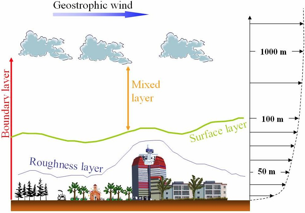
We consider our computational domain 𝒟𝒟\mathcal{D} in the neutral atmospheric boundary layer such as drawn in Figure 1. From floor to top, the height of 𝒟𝒟\mathcal{D} is at most the approximate size of the atmospheric boundary layer, namely 600600600 to 100010001000 m (in Section 5, we shall perform our numerical simulations for a domain 𝒟𝒟\mathcal{D} of height 300 m and 750 m).

Refer to caption

Figure 1: Schematic view of the atmosperic boundary layer. Courtesy of P. Drobinski [9].

We now detail the generic terms G𝐺G, C𝐶C in (2.1)–(2.2), and boundary conditions Uextsubscript𝑈ext{U_{\textrm{ext}}} in order to model the atmospheric boundary layer. In what follows, all the Eulerian averages {{\displaystyle{\langle}{~{}}\displaystyle{\rangle}}} are in the sense of (1.2).

Turbulence modeling

We use the classical notation for the velocity components (with numbering or with letters, depending on how it is convenient in the equations)

Ut=(ut(1),ut(2),ut(3))=(ut,vt,wt).subscriptU𝑡subscriptsuperscript𝑢1𝑡subscriptsuperscript𝑢2𝑡subscriptsuperscript𝑢3𝑡subscript𝑢𝑡subscript𝑣𝑡subscript𝑤𝑡{\rm U}_{t}=(u^{(1)}_{t},u^{(2)}_{t},u^{(3)}_{t})=(u_{t},v_{t},w_{t}).

Also for the components of the instantaneous turbulent velocity,

UtU(t,Xt)=(ut(1),ut(2),ut(3))=(ut,vt,wt),subscriptU𝑡delimited-⟨⟩U𝑡subscriptX𝑡subscriptsuperscript𝑢1𝑡subscriptsuperscript𝑢2𝑡subscriptsuperscript𝑢3𝑡superscriptsubscript𝑢𝑡superscriptsubscript𝑣𝑡superscriptsubscript𝑤𝑡{\rm U}_{t}-{{\displaystyle{\langle}{{\rm U}}\displaystyle{\rangle}}}(t,{\rm X}_{t})=(u^{\prime(1)}_{t},u^{\prime(2)}_{t},u^{\prime(3)}_{t})=(u_{t}^{\prime},v_{t}^{\prime},w_{t}^{\prime}),

for the turbulent kinetic energy (tke),

k(t,x)=12(utut+vtvt+wtwt),𝑘𝑡x12delimited-⟨⟩superscriptsubscript𝑢𝑡superscriptsubscript𝑢𝑡delimited-⟨⟩superscriptsubscript𝑣𝑡superscriptsubscript𝑣𝑡delimited-⟨⟩superscriptsubscript𝑤𝑡superscriptsubscript𝑤𝑡{k}(t,{\rm x})=\frac{1}{2}\left({{\displaystyle{\langle}{u_{t}^{\prime}u_{t}^{\prime}}\displaystyle{\rangle}}}+{{\displaystyle{\langle}{v_{t}^{\prime}v_{t}^{\prime}}\displaystyle{\rangle}}}+{{\displaystyle{\langle}{w_{t}^{\prime}w_{t}^{\prime}}\displaystyle{\rangle}}}\right),

and for 𝒫=12(𝒫11+𝒫22+𝒫33)𝒫12subscript𝒫11subscript𝒫22subscript𝒫33\mathcal{P}=\frac{1}{2}(\mathcal{P}_{11}+\mathcal{P}_{22}+\mathcal{P}_{33}), the rate of turbulent energy production, with

𝒫ij:=k=13(u(i)u(k)u(j)xk+u(j)u(k)u(i)xk).assignsubscript𝒫𝑖𝑗superscriptsubscript𝑘13delimited-⟨⟩superscript𝑢𝑖superscript𝑢𝑘delimited-⟨⟩superscript𝑢𝑗subscript𝑥𝑘delimited-⟨⟩superscript𝑢𝑗superscript𝑢𝑘delimited-⟨⟩superscript𝑢𝑖subscript𝑥𝑘\displaystyle\mathcal{P}_{ij}:=-\sum_{k=1}^{3}\left({{\displaystyle{\langle}{u^{\prime(i)}u^{\prime(k)}}\displaystyle{\rangle}}}\dfrac{\partial{{\displaystyle{\langle}{u^{(j)}}\displaystyle{\rangle}}}}{\partial x_{k}}+{{\displaystyle{\langle}{u^{\prime(j)}u^{\prime(k)}}\displaystyle{\rangle}}}\dfrac{\partial{{\displaystyle{\langle}{u^{(i)}}\displaystyle{\rangle}}}}{\partial x_{k}}\right).

Turbulence models roughly consist in linking the turbulent kinetic energy k𝑘{k} and the turbulent energy dissipation ε𝜀\varepsilon. In order to account for turbulence effects in the Lagrangian velocity equation (2.1b), we define its coefficients as:

C(t,x)=C0ε(t,x),𝐶𝑡xsubscript𝐶0𝜀𝑡x\displaystyle C(t,{\rm x})=\sqrt{C_{0}\,\varepsilon(t,{\rm x})}, (2.11a)
Gi,j(t,x)=CR2ε(t,x)k(t,x)δij+C2u(i)xj(t,x).subscript𝐺𝑖𝑗𝑡xsubscript𝐶𝑅2𝜀𝑡x𝑘𝑡xsubscript𝛿𝑖𝑗subscript𝐶2delimited-⟨⟩superscript𝑢𝑖subscript𝑥𝑗𝑡x\displaystyle G_{i,j}(t,{\rm x})=-\frac{C_{R}}{2}\dfrac{\varepsilon(t,{\rm x})}{{k}(t,{\rm x})}\delta_{ij}+C_{2}\dfrac{\partial{{\displaystyle{\langle}{u^{(i)}}\displaystyle{\rangle}}}}{\partial x_{j}}(t,{\rm x}). (2.11b)

The tensor Gi,jsubscript𝐺𝑖𝑗G_{i,j} is related to the isotropization of turbulence production model (IP model) that accounts to the Reynolds-stress anisotropies (see Durbin and Speziale [11] and [25] ) and C0subscript𝐶0C_{0} is given by

C0=23(CR+C2𝒫ε1).subscript𝐶023subscript𝐶𝑅subscript𝐶2𝒫𝜀1\displaystyle C_{0}=\frac{2}{3}\left(C_{R}+C_{2}\frac{\mathcal{P}}{\varepsilon}-1\right). (2.12)

The turbulent energy dissipation ε(t,x)𝜀𝑡x\varepsilon(t,{\rm x}) is recovered via the turbulent kinetic energy as a parametrization (see Drobinski et al. [10]),

ε(t,x)=Cεk3/2(t,x)m(x).𝜀𝑡xsubscript𝐶𝜀superscript𝑘32𝑡xsubscriptmx\varepsilon(t,{\rm x})=C_{\varepsilon}\,\dfrac{k^{3/2}(t,{\rm x})}{\ell_{\textrm{m}}({\rm x})}. (2.13)

It is worth to notice that the term ε(t,x)/k(t,x)𝜀𝑡x𝑘𝑡x\varepsilon(t,{\rm x})/k(t,{\rm x}) in the Gi,jsubscript𝐺𝑖𝑗G_{i,j} tensor is Cεk1/2(t,x)m(x)subscript𝐶𝜀superscript𝑘12𝑡xsubscriptmxC_{\varepsilon}\,\dfrac{k^{1/2}(t,{\rm x})}{\ell_{\textrm{m}}({\rm x})}. Thus when the turbulent kinetic energy k𝑘{k} vanishes, all the terms in the particles dynamics (2.5, 2.11) stay well defined. As a local model, possibly forced by dynamical boundary condition as in [3] or by a log law wind profile as in the following Sections 4 and 5, SDM is mainly pertinent in the turbulent part of the atmosphere. However, it can be observed that SDM well reproduces the decay of the turbulent kinetic energy in the boundary layer, and up to the geostrophic height, making vanished the tke k𝑘{k} at the top, where the flow becomes laminar (see Figure 15).

The mixing length msubscriptm\ell_{\textrm{m}} can be considered as constant away from the floor (above the surface layer). However, as can be seen in Carlotti [7], it should be proportional to the vertical coordinate z𝑧z within the surface layer. A classical choice consists in a piecewise linear function for msubscriptm\ell_{\textrm{m}} proportional to von Karman constant κ𝜅\kappa:

m(z)=κ(zzm)𝟙[0,zm](z)+κzm.subscriptm𝑧𝜅𝑧subscript𝑧subscriptmsubscript10subscript𝑧subscriptm𝑧𝜅subscript𝑧subscriptm\displaystyle\ell_{\textrm{m}}(z)=\kappa(z-z_{\ell_{\textrm{m}}}){\mathds{1}}_{[0,z_{\ell_{\textrm{m}}}]}(z)+\kappa z_{\ell_{\textrm{m}}}. (2.14)

Putting together (1.2),(2.11) with the generic Eulerian average approximation formula (2.7), we obtain the following expression for the turbulent characteristics computed by SDM:

k(t,x)12(uu(t,x)+vv(t,x)+ww(t,x)).𝒫ijk=13(u(i)u(k)u(j)xk+u(j)u(k)u(i)xk)Gi,j(t,x)CR2Cεk1/2(t,x)m(x)δij+C2u(i)xj(t,x).𝑘𝑡xsimilar-to-or-equalsabsent12delimited-⟨⟩delimited-⟨⟩superscript𝑢superscript𝑢𝑡xdelimited-⟨⟩delimited-⟨⟩superscript𝑣superscript𝑣𝑡xdelimited-⟨⟩delimited-⟨⟩superscript𝑤superscript𝑤𝑡xsubscript𝒫𝑖𝑗similar-to-or-equalsabsentsuperscriptsubscript𝑘13delimited-⟨⟩delimited-⟨⟩superscript𝑢𝑖superscript𝑢𝑘delimited-⟨⟩delimited-⟨⟩superscript𝑢𝑗subscript𝑥𝑘delimited-⟨⟩delimited-⟨⟩superscript𝑢𝑗superscript𝑢𝑘delimited-⟨⟩delimited-⟨⟩superscript𝑢𝑖subscript𝑥𝑘subscript𝐺𝑖𝑗𝑡xsimilar-to-or-equalsabsentsubscript𝐶𝑅2subscript𝐶𝜀superscript𝑘12𝑡xsubscriptmxsubscript𝛿𝑖𝑗subscript𝐶2delimited-⟨⟩delimited-⟨⟩superscript𝑢𝑖subscript𝑥𝑗𝑡x\displaystyle\begin{aligned} k(t,{\rm x})&\simeq\frac{1}{2}\left({{\displaystyle{\langle}\!\>\!\!{\langle}{u^{\prime}u^{\prime}}\displaystyle{\rangle}\!\>\!\!{\rangle}}}(t,{\rm x})+{{\displaystyle{\langle}\!\>\!\!{\langle}{v^{\prime}v^{\prime}}\displaystyle{\rangle}\!\>\!\!{\rangle}}}(t,{\rm x})+{{\displaystyle{\langle}\!\>\!\!{\langle}{w^{\prime}w^{\prime}}\displaystyle{\rangle}\!\>\!\!{\rangle}}}(t,{\rm x})\right).\\ \mathcal{P}_{ij}&\simeq-\sum_{k=1}^{3}\left({{\displaystyle{\langle}\!\>\!\!{\langle}{u^{\prime(i)}u^{\prime(k)}}\displaystyle{\rangle}\!\>\!\!{\rangle}}}\dfrac{\partial{{\displaystyle{\langle}\!\>\!\!{\langle}{u^{(j)}}\displaystyle{\rangle}\!\>\!\!{\rangle}}}}{\partial x_{k}}+{{\displaystyle{\langle}\!\>\!\!{\langle}{u^{\prime(j)}u^{\prime(k)}}\displaystyle{\rangle}\!\>\!\!{\rangle}}}\dfrac{\partial{{\displaystyle{\langle}\!\>\!\!{\langle}{u^{(i)}}\displaystyle{\rangle}\!\>\!\!{\rangle}}}}{\partial x_{k}}\right)\\ G_{i,j}(t,{\rm x})&\simeq-\frac{C_{R}}{2}C_{\varepsilon}\,\dfrac{k^{1/2}(t,{\rm x})}{\ell_{\textrm{m}}({\rm x})}\delta_{ij}+C_{2}\dfrac{\partial{{\displaystyle{\langle}\!\>\!\!{\langle}{u^{(i)}}\displaystyle{\rangle}\!\>\!\!{\rangle}}}}{\partial x_{j}}(t,{\rm x}).\end{aligned} (2.15)

Boundary conditions

As can be seen in Figure 1, our computational domain is bounded from above by the free troposhere where a geostrophic balance can be considered. As a consequence, we shall use Dirichlet boundary conditions at the top of the domain,

U(t,x)=UG(t,x),delimited-⟨⟩U𝑡xsubscript𝑈𝐺𝑡x{{\displaystyle{\langle}{{\rm U}}\displaystyle{\rangle}}}(t,{\rm x})=U_{G}(t,{\rm x}), (2.16)

where UGsubscript𝑈𝐺U_{G} is given, corresponding to the output of a geostrophic model.

The bottom boundary condition should account for the surface roughness and corresponding layer: we incorporate a log law in our model, such as described in the forthcoming section.

Finally, since we want to model one or several mills we propose to use inflow (log law profile) and outflow (free output) boundary conditions for the (x,y)𝑥𝑦(x,y) lateral frontiers, as described in Section 5 below.

2.4 Wall-boundary condition

For the modeling effect of the ground, we borrow and adapt the particle boundary condition proposed by Minier and Pozorski [23] that aims to reproduce the momentum exchange between the ground and the bulk of the flow. This method is equivalent to wall functions approach in classical turbulence models.

Here, we just resume the main idea in [23] which consists in imposing a reflection to the particle trajectories, when it arrive to a given height zmirrorsubscript𝑧mirrorz_{\textrm{mirror}}, where zmirrorsubscript𝑧mirrorz_{\textrm{mirror}} is chosen in the logarithmic layer.

In order to define the reflection of the particles on this mirror face {z=zmirror}𝑧subscript𝑧mirror\{z=z_{\textrm{mirror}}\}, we denote with a ‘in’ the inward velocities in the region {z[zmirror,H]}𝑧subscript𝑧mirror𝐻\{z\in[z_{\textrm{mirror}},H]\} and with a ‘out’ the outward velocities in the region {z[0,zmirror]}𝑧0subscript𝑧mirror\{z\in[0,z_{\textrm{mirror}}]\}.

The velocity Uinsubscript𝑈inU_{\textrm{in}} is oriented to the top whereas Uoutsubscript𝑈outU_{\textit{out}} is oriented to the bottom. A symmetry principle allows to replace any outward particle to its mirror inward particle.

\bulletCell centerCells{z=zc}𝑧subscript𝑧c\{z=z_{\textrm{c}}\}Outward particle\bulletUoutsubscriptUout{\rm U}_{\textit{out}}UinsubscriptUin{\rm U}_{\textrm{in}}\bulletMirror particle{z=zmirror}𝑧subscript𝑧mirror\{z=z_{\textrm{mirror}}\}{z=z0}𝑧subscript𝑧0\{z=z_{0}\}{z=0}𝑧0\{z=0\}Ground
Figure 2: The mirror reflection scheme for the velocity near the ground.

The vertical component is simply reflected at zmirrorsubscript𝑧mirrorz_{\textrm{mirror}}:

win=woutsubscript𝑤insubscript𝑤out\displaystyle w_{\textrm{in}}=-w_{\textit{out}} (2.17)

whereas the horizontal velocity are lifted in a way that preserves the covariances uwdelimited-⟨⟩superscript𝑢superscript𝑤{{\displaystyle{\langle}{u^{\prime}w^{\prime}}\displaystyle{\rangle}}} and vwdelimited-⟨⟩superscript𝑣superscript𝑤{{\displaystyle{\langle}{v^{\prime}w^{\prime}}\displaystyle{\rangle}}} in this reflection process:

uin=uout2uww2wout,subscript𝑢insubscript𝑢out2delimited-⟨⟩superscript𝑢superscript𝑤delimited-⟨⟩superscript𝑤2subscript𝑤out\displaystyle u_{\textrm{in}}=u_{\textit{out}}-2\frac{{{\displaystyle{\langle}{u^{\prime}w^{\prime}}\displaystyle{\rangle}}}}{{{\displaystyle{\langle}{w^{\prime 2}}\displaystyle{\rangle}}}}\,w_{\textit{out}}, (2.18)
vin=vout2vww2wout.subscript𝑣insubscript𝑣out2delimited-⟨⟩superscript𝑣superscript𝑤delimited-⟨⟩superscript𝑤2subscript𝑤out\displaystyle v_{\textrm{in}}=v_{\textit{out}}-2\frac{{{\displaystyle{\langle}{v^{\prime}w^{\prime}}\displaystyle{\rangle}}}}{{{\displaystyle{\langle}{w^{\prime 2}}\displaystyle{\rangle}}}}\,w_{\textit{out}}. (2.19)

It remains to impose the covariances at the ground.

In [7], Carlotti describes the method used in the Meso-NH model [17] for the account of the log law. This method is inspired from the one of Schmid and Schumann [29]: the boundary condition for the subgrid covariances uwdelimited-⟨⟩superscript𝑢superscript𝑤{{\displaystyle{\langle}{u^{\prime}w^{\prime}}\displaystyle{\rangle}}} and vwdelimited-⟨⟩superscript𝑣superscript𝑤{{\displaystyle{\langle}{v^{\prime}w^{\prime}}\displaystyle{\rangle}}} are fixed to

uw(t,x,y)delimited-⟨⟩superscript𝑢superscript𝑤𝑡𝑥𝑦\displaystyle{{\displaystyle{\langle}{u^{\prime}w^{\prime}}\displaystyle{\rangle}}}(t,x,y) =\displaystyle= (uu2+v2u2)(t,x,y)delimited-⟨⟩𝑢superscriptdelimited-⟨⟩𝑢2superscriptdelimited-⟨⟩𝑣2superscriptsubscript𝑢2𝑡𝑥𝑦\displaystyle-\left(\frac{{{\displaystyle{\langle}{u}\displaystyle{\rangle}}}}{\sqrt{{{\displaystyle{\langle}{u}\displaystyle{\rangle}}}^{2}+{{\displaystyle{\langle}{v}\displaystyle{\rangle}}}^{2}}}u_{*}^{2}\right)(t,x,y) (2.20)
vw(t,x,y)delimited-⟨⟩superscript𝑣superscript𝑤𝑡𝑥𝑦\displaystyle{{\displaystyle{\langle}{v^{\prime}w^{\prime}}\displaystyle{\rangle}}}(t,x,y) =\displaystyle= (vu2+v2u2)(t,x,y)delimited-⟨⟩𝑣superscriptdelimited-⟨⟩𝑢2superscriptdelimited-⟨⟩𝑣2superscriptsubscript𝑢2𝑡𝑥𝑦\displaystyle-\left(\frac{{{\displaystyle{\langle}{v}\displaystyle{\rangle}}}}{\sqrt{{{\displaystyle{\langle}{u}\displaystyle{\rangle}}}^{2}+{{\displaystyle{\langle}{v}\displaystyle{\rangle}}}^{2}}}u_{*}^{2}\right)(t,x,y) (2.21)

where the friction velocity usubscript𝑢u_{*}333u=(uw2+vw2)1/4subscript𝑢superscriptsuperscriptdelimited-⟨⟩superscript𝑢superscript𝑤2superscriptdelimited-⟨⟩superscript𝑣superscript𝑤214u_{*}=\left({{\displaystyle{\langle}{u^{\prime}w^{\prime}}\displaystyle{\rangle}}}^{2}+{{\displaystyle{\langle}{v^{\prime}w^{\prime}}\displaystyle{\rangle}}}^{2}\right)^{1/4}. is computed in each cell at the bottom of the domain using the log law

u(t,xc,yc)=κu2(t,xc,yc,zc)+v2(t,xc,yc,zc)log(zcz0)subscript𝑢𝑡subscript𝑥csubscript𝑦c𝜅superscriptdelimited-⟨⟩𝑢2𝑡subscript𝑥csubscript𝑦csubscript𝑧csuperscriptdelimited-⟨⟩𝑣2𝑡subscript𝑥csubscript𝑦csubscript𝑧csubscript𝑧csubscript𝑧0\displaystyle u_{*}(t,x_{\textrm{c}},y_{\textrm{c}})=\kappa\frac{\sqrt{{{\displaystyle{\langle}{u}\displaystyle{\rangle}}}^{2}(t,x_{\textrm{c}},y_{\textrm{c}},z_{\textrm{c}})+{{\displaystyle{\langle}{v}\displaystyle{\rangle}}}^{2}(t,x_{\textrm{c}},y_{\textrm{c}},z_{\textrm{c}})}}{\log\displaystyle\left(\frac{z_{\textrm{c}}}{z_{0}}\right)} (2.22)

where κ𝜅\kappa is the von Karmann constant, z0subscript𝑧0z_{0} is the roughness length parameter, and (xc,yc,zc)subscript𝑥csubscript𝑦csubscript𝑧c(x_{\textrm{c}},y_{\textrm{c}},z_{\textrm{c}}) is the position of a cell’s center, for the cells on the floor.

We adapt this idea in SDM with the following steps.

Step 1.

Given u(tn)delimited-⟨⟩𝑢subscript𝑡𝑛{{\displaystyle{\langle}{u}\displaystyle{\rangle}}}(t_{n}) and v(tn)delimited-⟨⟩𝑣subscript𝑡𝑛{{\displaystyle{\langle}{v}\displaystyle{\rangle}}}(t_{n}), for any of the cells on the floor,
- we compute u(tn,xc,yc)subscript𝑢subscript𝑡𝑛subscript𝑥csubscript𝑦cu_{*}(t_{n},x_{\textrm{c}},y_{\textrm{c}}) with (2.22)
- we compute uw(tn,xc,yc)delimited-⟨⟩superscript𝑢superscript𝑤subscript𝑡𝑛subscript𝑥csubscript𝑦c{{\displaystyle{\langle}{u^{\prime}w^{\prime}}\displaystyle{\rangle}}}(t_{n},x_{\textrm{c}},y_{\textrm{c}}) and vw(tn,xc,yc)delimited-⟨⟩superscript𝑣superscript𝑤subscript𝑡𝑛subscript𝑥csubscript𝑦c{{\displaystyle{\langle}{v^{\prime}w^{\prime}}\displaystyle{\rangle}}}(t_{n},x_{\textrm{c}},y_{\textrm{c}}) using (2.20) and (2.21).

Step 2.

For the particle boundary condition at zmirrorsubscript𝑧mirrorz_{\textrm{mirror}}, we localize the particle crossing the interface in the cell of center (xc,yc,zc)subscript𝑥csubscript𝑦csubscript𝑧c(x_{\textrm{c}},y_{\textrm{c}},z_{\textrm{c}}); we use uw(tn,xc,yc)delimited-⟨⟩superscript𝑢superscript𝑤subscript𝑡𝑛subscript𝑥csubscript𝑦c{{\displaystyle{\langle}{u^{\prime}w^{\prime}}\displaystyle{\rangle}}}(t_{n},x_{\textrm{c}},y_{\textrm{c}}) and vw(tn,xc,yc)delimited-⟨⟩superscript𝑣superscript𝑤subscript𝑡𝑛subscript𝑥csubscript𝑦c{{\displaystyle{\langle}{v^{\prime}w^{\prime}}\displaystyle{\rangle}}}(t_{n},x_{\textrm{c}},y_{\textrm{c}}) to compute the reflected velocity of the mirror particle at the interface, using (2.17), (2.18) and (2.19).

In [23], the authors propose to fix zmirrorsubscript𝑧mirrorz_{\textrm{mirror}} to 35zc35subscript𝑧c\frac{3}{5}z_{\textrm{c}}. In our simulations in the following sections, we used zmirror=12zcsubscript𝑧mirror12subscript𝑧cz_{\textrm{mirror}}=\frac{1}{2}z_{\textrm{c}}.

3 Actuator disc methods in the Lagrangian setting

The presence of wind mills is taken into account thanks to additional force terms in the stochastic differential equations that govern the movement of the particles. To this end, equation (2.1b) (which governs the time evolution of the velocity Ut=(ut,vt,wt)subscriptU𝑡subscript𝑢𝑡subscript𝑣𝑡subscript𝑤𝑡{\rm U}_{t}=\left(u_{t},v_{t},w_{t}\right) of a particle) is modified as follows:

dUt=𝑑subscriptU𝑡absent\displaystyle d{\rm U}_{t}= (1ρx𝒫(t,Xt))dt1𝜌subscript𝑥𝒫𝑡subscriptX𝑡𝑑𝑡\displaystyle\left(-\frac{1}{\rho}\nabla_{x}{{\displaystyle{\langle}{{\mathscr{P}}}\displaystyle{\rangle}}}(t,{\rm X}_{t})\right)dt (3.1)
G(t,Xt)(UtU(t,Xt))dt+C(t,Xt)dWt𝐺𝑡subscriptX𝑡subscriptU𝑡delimited-⟨⟩U𝑡subscriptX𝑡𝑑𝑡𝐶𝑡subscriptX𝑡𝑑subscript𝑊𝑡\displaystyle-G(t,{\rm X}_{t})\Big{(}{\rm U}_{t}-{{\displaystyle{\langle}{{\rm U}}\displaystyle{\rangle}}}(t,{\rm X}_{t})\Big{)}dt+C(t,{\rm X}_{t})dW_{t}
+f(t,Xt,Ut)dt+fnacelle(t,Xt,Ut)dt+fmast(t,Xt,Ut)dt.𝑓𝑡subscriptX𝑡subscriptU𝑡𝑑𝑡subscript𝑓nacelle𝑡subscriptX𝑡subscriptU𝑡𝑑𝑡subscript𝑓mast𝑡subscriptX𝑡subscriptU𝑡𝑑𝑡\displaystyle+f\left(t,{\rm X}_{t},{\rm U}_{t}\right)dt+f_{\textit{nacelle}}\left(t,{\rm X}_{t},{\rm U}_{t}\right)dt+f_{\textit{mast}}\left(t,{\rm X}_{t},{\rm U}_{t}\right)dt.

The term f(t,Xt,Ut)𝑓𝑡subscriptX𝑡subscriptU𝑡f\left(t,{\rm X}_{t},{\rm U}_{t}\right) represents the body forces that the blades exert on the flow. The supplementary terms fnacelle(t,Xt,Ut)subscript𝑓nacelle𝑡subscriptX𝑡subscriptU𝑡f_{\textit{nacelle}}\left(t,{\rm X}_{t},{\rm U}_{t}\right) and fmast(t,Xt,Ut)subscript𝑓mast𝑡subscriptX𝑡subscriptU𝑡f_{\textit{mast}}\left(t,{\rm X}_{t},{\rm U}_{t}\right) represent the impact of the mill nacelle and mast. In the present work, only the blade and nacelle forces are considered.

In this section, we discuss how those force terms should be implemented in the Lagrangian setting considered here, in order to recover consistency with classical Eulerian formulations.

Considering the full geometrical description of the blades (that requires a very fine mesh), the force f𝑓f is a very complex function which encodes the geometry of the blades; however, in this study we are interested in the overall impact of the mills in the flow, and not in the fine geometrical details of the reciprocal interactions. For this reason, and to avoid costly computations, an actuator disc approach is used to provide approximations of f𝑓f, with two different levels of complexity:

  • (a)

    Non-rotating actuator disc with uniform loading.

  • (b)

    Rotating actuator disc.

In the Actuator Disc approach, each mill is represented as an immersed surface which concentrates all forces exerted by the mill on the flow. A thorough description of this methodology can be found in Mikkelsen [20], and in the books by Hansen [14] and Manwell, McGowan and Rogers [18]. With different degrees of complexity, it has been applied to wind turbine simulations in Porté-Agel, Lub and Wu [26], Master et al. [19], El Kasmi and Masson [12]. It has also been used to simulate arrays of turbines in Wu and Porté-Agel [33].
Refer to caption
(a) Local coordinates
Refer to caption
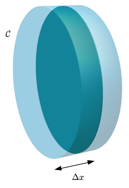
(b) The cylinder 𝒞𝒞\mathcal{C}
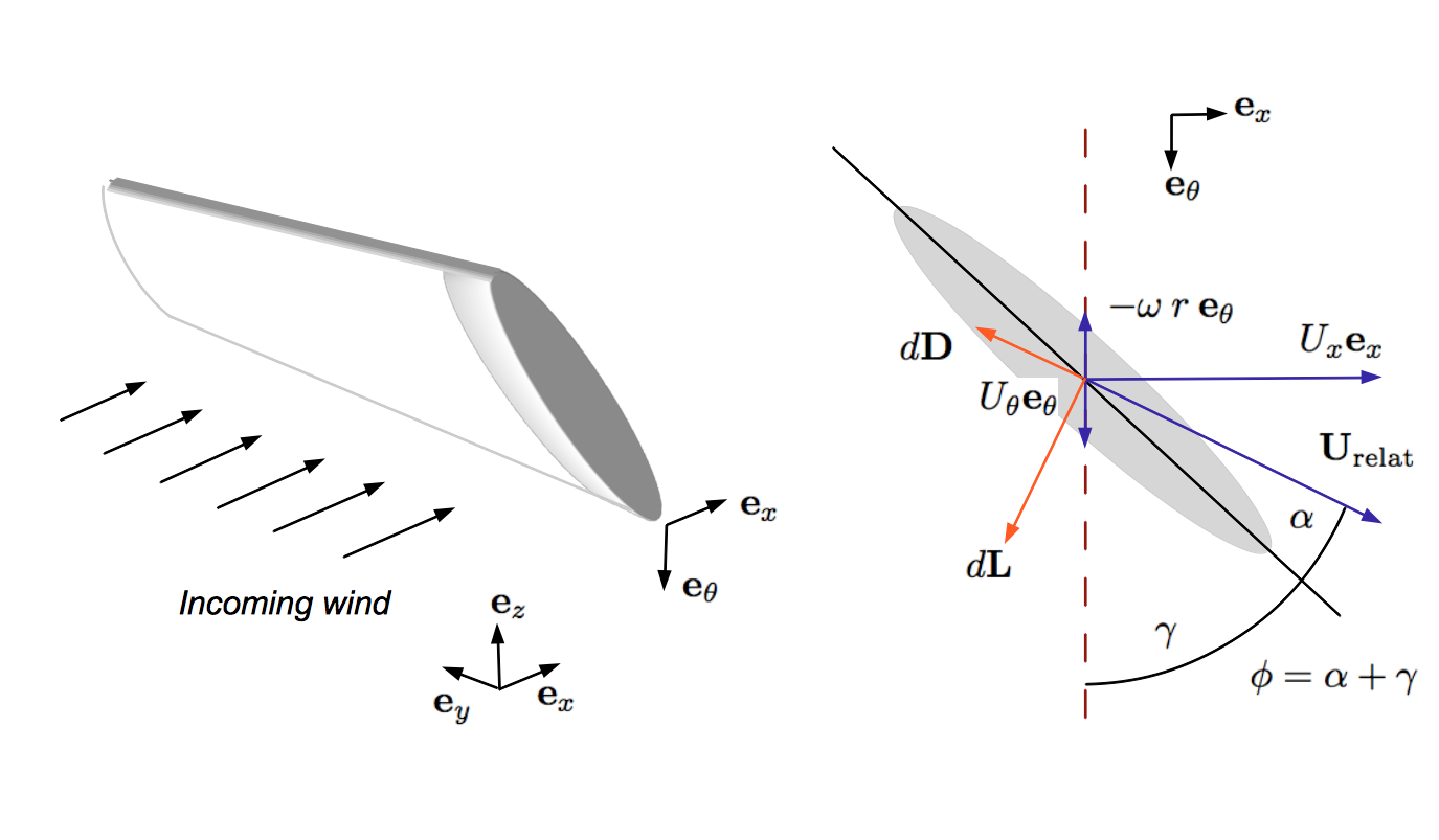
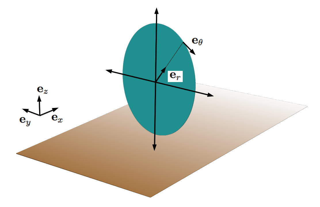
Figure 3: (a) The local reference frame at the actuator disc of the turbine, using cylindrical coordinates.
(b) The cylinder 𝒞𝒞\mathcal{C} that extends the actuator disc. Mill forces are applied to particles that lie inside.

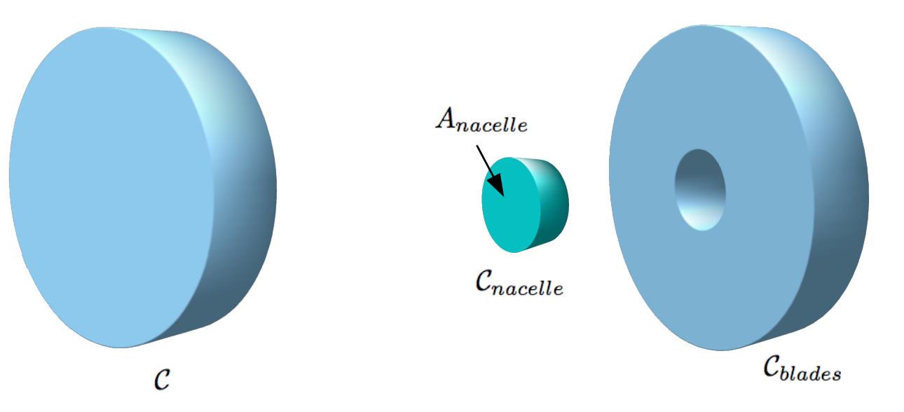
It is assumed that the flow moves along the positive direction of the x𝑥x axis, and that the turbine’s main axis is aligned with the x𝑥x axis, so that it faces the wind directly. It is convenient to define local reference frame of cylindrical coordinates centered at the hub of the turbine, with basis vectors 𝐞xsubscript𝐞𝑥{\bf{e}}_{x}, 𝐞rsubscript𝐞𝑟{\bf{e}}_{r} and 𝐞θsubscript𝐞𝜃{\bf{e}}_{\theta} as shown in Figure 3a. In order to apply the forces to the particles, the actuator disc is expanded to a cylinder 𝒞𝒞\mathcal{C} of depth ΔxΔ𝑥\Delta x, and the forces per unit mass are used to correct the velocities of all particles lying inside 𝒞𝒞\mathcal{C}. This cylinder is divided in two regions: 𝒞=𝒞blades𝒞nacelle𝒞subscript𝒞bladessubscript𝒞nacelle\mathcal{C}=\mathcal{C}_{\textit{blades}}\cup\mathcal{C}_{\textit{nacelle}}, as depicted in Figure 4, where 𝒞bladessubscript𝒞blades\mathcal{C}_{\textit{blades}} represents the region occupied by the blades, and 𝒞nacellesubscript𝒞nacelle\mathcal{C}_{\textit{nacelle}} represents the region occupied by the nacelle. For the two models considered here (non-rotating and rotating actuator disc), the force term f𝑓f is computed for and applied to particles lying inside region 𝒞bladessubscript𝒞blades\mathcal{C}_{\textit{blades}}; and correspondingly, the term fnacellesubscript𝑓nacellef_{\textit{nacelle}} is computed for and applied to particles lying inside region 𝒞nacellesubscript𝒞nacelle\mathcal{C}_{\textit{nacelle}}. The following sections describe the way in which this is done.
Refer to caption
Figure 4: Left: cylinder 𝒞𝒞\mathcal{C} representing the turbine. Right: sub-regions corresponding to the nacelle and blades, viewed by particles.

In the rest of this section we discuss successively on the force f𝑓f in the non rotating actuator disc model, and in the rotating actuator disc model. We end by considering the fnacellesubscript𝑓nacellef_{\textit{nacelle}}.

3.1 Non rotating, uniformly loaded actuator disc model

In this model, the turbine force corresponding to the blades is distributed uniformly over the region 𝒞bladessubscript𝒞blades\mathcal{C}_{\textit{blades}}, and rotational effects are ignored. In the simplest formulation of the model, for a turbine facing a uniform laminar steady state flow, and ignoring the influence of the nacelle, the total thrust force exerted by the turbine is given by an expression of the form

Fx=12ρACTU2𝐞x,subscript𝐹𝑥12𝜌𝐴subscript𝐶𝑇superscriptsubscript𝑈2subscript𝐞𝑥F_{x}=-\frac{1}{2}\rho AC_{T}U_{\infty}^{2}{\bf{e}}_{x},

where 𝐔subscript𝐔{\mathbf{U}}_{\infty} is the unperturbed velocity far upstream from the turbine’s location, Usubscript𝑈U_{\infty} is its norm, A𝐴A is the surface area of the turbine’s disc, ρ𝜌\rho is the density of air, and CTsubscript𝐶𝑇C_{T} is a dimensionless, flow dependent parameter called the thrust coefficient.

An elementary deduction of this expression can be found in [14] or [18]. This deduction, which is essentially one-dimensional, is based on conservation of linear momentum for a stream tube passing through the turbine’s disc (see Figure 5). The analysis assumes that the turbine faces uniform, inviscid, steady-state flow, and hence there is radial symmetry with respect to the hub of the turbine. Further, a constant loading is assumed at the disc, and thus the velocity field is constant and uniform there. The thrust coefficient CTsubscript𝐶𝑇C_{T} is specified in terms of the axial induction factor a𝑎a,

a=UUDU,𝑎subscript𝑈subscript𝑈𝐷subscript𝑈a=\frac{U_{\infty}-U_{D}}{U_{\infty}}, (3.2)

which measures the relative decrease in speed from the far upstream region and the disc region, where the local velocity has magnitude UD<Usubscript𝑈𝐷subscript𝑈U_{D}<U_{\infty} (see Figure 5).

Refer to caption
Figure 5: A stream tube passing through the actuator disc of the turbine. Uniform flow is assumed at the far upstream region.

As in Réthoré et al. [28], the local velocity magnitude UDsubscript𝑈𝐷U_{D} (whose exact formula is yet to be specified) is used instead of Usubscript𝑈U_{\infty} by combining (3.2) with the thrust force expression that becomes

Fx=2ρa(1a)AUD2𝐞x,subscript𝐹𝑥2𝜌𝑎1𝑎𝐴superscriptsubscript𝑈𝐷2subscript𝐞𝑥F_{x}=-2\rho\dfrac{a}{(1-a)}AU_{D}^{2}{\bf{e}}_{x}, (3.3)

and

CT=4a(1a).subscript𝐶𝑇4𝑎1𝑎C_{T}=4a(1-a). (3.4)

In order to adapt this thrust force model to particles, the disc is extended to a cylinder 𝒞𝒞\mathcal{C} of length ΔxΔ𝑥\Delta x and mass ρAΔx𝜌𝐴Δ𝑥\rho A\Delta x (see Figure 3b), which is subdivided in the two regions 𝒞bladessubscript𝒞blades\mathcal{C}_{\textit{blades}} and 𝒞nacellesubscript𝒞nacelle\mathcal{C}_{\textit{nacelle}}, as depicted in Figure 4. In both cases, the force is assumed to be uniformly distributed along the additional dimension. In the present section, we restrict ourselves to the adaptation of the model to the region 𝒞bladessubscript𝒞blades\mathcal{C}_{\textit{blades}}. The force per unit mass inside region 𝒞bladessubscript𝒞blades\mathcal{C}_{\textit{blades}} is then given by:

fx=1Δx2a1aUD2𝟙{x𝒞blades}𝐞x.subscript𝑓𝑥1Δ𝑥2𝑎1𝑎superscriptsubscript𝑈𝐷2subscript1𝑥subscript𝒞bladessubscript𝐞𝑥f_{x}=-\frac{1}{\Delta x}\frac{2a}{1-a}U_{D}^{2}{\mathds{1}}_{\{x\in\mathcal{C}_{\textit{blades}}\}}{\bf{e}}_{x}. (3.5)

As soon as we have specified how UDsubscript𝑈𝐷U_{D} is computed for each individual particle, from (3.5) follows Algorithm 2, for a given time step of length ΔtΔ𝑡\Delta t beginning at time tnsubscript𝑡𝑛t_{n}, and a given particle with position XtnsubscriptXsubscript𝑡𝑛{\rm X}_{t_{n}} and velocity UtnsubscriptUsubscript𝑡𝑛{\rm U}_{t_{n}} at time tnsubscript𝑡𝑛t_{n}.

Algorithm 2 -- Update the Lagrangian velocity with thrust force in the non rotating actuator disc model.
  PRESTEP Compute the mean local speed at the disc UD(Lagrangian)superscriptsubscript𝑈𝐷(Lagrangian)U_{D}^{\textrm{\tiny(Lagrangian)}}
  if Xtn𝒞bladessubscriptXsubscript𝑡𝑛subscript𝒞blades{\rm X}_{t_{n}}\in\mathcal{C}_{\textit{blades}} then
     Utn+1Utn+11Δx2a1a(UD(Lagrangian))2𝐞xΔt.maps-tosubscriptUsubscript𝑡𝑛1subscriptUsubscript𝑡𝑛11Δ𝑥2𝑎1𝑎superscriptsuperscriptsubscript𝑈𝐷(Lagrangian)2subscript𝐞𝑥Δ𝑡{\rm U}_{t_{n+1}}\mapsto{\rm U}_{t_{n+1}}-\frac{1}{\Delta x}\frac{2a}{1-a}\left(U_{D}^{\textrm{\tiny(Lagrangian)}}\right)^{2}\;{\bf{e}}_{x}\;\Delta t.
  end if

Since (3.5) is derived from a laminar one-dimensional analysis, its generalization to turbulent shear flow requires UD(Lagrangian)superscriptsubscript𝑈𝐷(Lagrangian)U_{D}^{\textrm{\tiny(Lagrangian)}} to be carefully specified. For a particle with position XtnsubscriptXsubscript𝑡𝑛{\rm X}_{t_{n}} in 𝒞bladessubscript𝒞blades\mathcal{C}_{\textit{blades}} and velocity UtnsubscriptUsubscript𝑡𝑛{\rm U}_{t_{n}} at time tnsubscript𝑡𝑛t_{n}, at least three possibilities exist (all equivalent for uniform, laminar, steady-state flows):

  • (a)

    define UD(Lagrangian)=|utn|superscriptsubscript𝑈𝐷(Lagrangian)subscript𝑢subscript𝑡𝑛U_{D}^{\textrm{\tiny(Lagrangian)}}=\left|u_{t_{n}}\right|;

  • (b)

    define UD(Lagrangian)=|u|(tn,Xtn)superscriptsubscript𝑈𝐷(Lagrangian)delimited-⟨⟩𝑢subscript𝑡𝑛subscriptXsubscript𝑡𝑛U_{D}^{\textrm{\tiny(Lagrangian)}}=\left|{{\displaystyle{\langle}{u}\displaystyle{\rangle}}}\right|(t_{n},{\rm X}_{t_{n}});

  • (c)

    compute UD(Lagrangian)superscriptsubscript𝑈𝐷(Lagrangian)U_{D}^{\textrm{\tiny(Lagrangian)}} as the magnitude of average velocity of particles inside cylinder 𝒞bladessubscript𝒞blades\mathcal{C}_{\textit{blades}}:

    UD(Lagrangian)=|𝔼[utn|Xtn𝒞blades]|.U_{D}^{\textrm{\tiny(Lagrangian)}}=\left|\displaystyle{\mathbb{E}}\left[u_{t_{n}}|{\rm X}_{t_{n}}\in\mathcal{C}_{\textit{blades}}\right]\right|. (3.6)

If one selects options (a), Equation (3.5) describes the instantaneous force, and not the mean one. Given the flow-dependent nature of the axial induction factor a𝑎a, and the fact that it pertains to the whole disc of the turbine, option (c) is adopted, preferably to option (b); the force density then becomes:

fx=1Δx2a1a|𝔼[ut|Xt𝒞blades]|2𝟙{Xt𝒞blades}𝐞x.subscript𝑓𝑥1Δ𝑥2𝑎1𝑎superscript𝔼delimited-[]conditionalsubscript𝑢𝑡subscriptX𝑡subscript𝒞blades2subscript1subscriptX𝑡subscript𝒞bladessubscript𝐞𝑥f_{x}=-\frac{1}{\Delta x}\frac{2a}{1-a}\big{\lvert}\displaystyle{\mathbb{E}}\left[u_{t}|{\rm X}_{t}\in\mathcal{C}_{\textit{blades}}\right]\big{\rvert}^{2}{\mathds{1}}_{\{{\rm X}_{t}\in\mathcal{C}_{\textit{blades}}\}}{\bf{e}}_{x}. (3.7)

3.2 Rotating actuator disc model

This model is based on a blade element analysis, which gives a description of the blade forces in terms of a set of simple geometrical parameters. The model assumes that each blade is comprised of tiny pieces (blade elements), each encompassing an infinitesimal length dr𝑑𝑟dr, which concentrate the relevant forces that the turbine exerts on the flow. It is assumed that these blade elements are independent of one another, in the sense that they do not induce any radial movement on the flow.

To be precise, consider the reference frame depicted in Figure 3a, with basis vectors 𝐞xsubscript𝐞𝑥{\bf{e}}_{x}, 𝐞rsubscript𝐞𝑟{\bf{e}}_{r}, 𝐞θsubscript𝐞𝜃{\bf{e}}_{\theta} along the axial (stream wise), radial and tangential directions, respectively. The corresponding flow velocity components in this frame will be denoted (Ux,Ur,Uθ)subscriptU𝑥subscriptU𝑟subscriptU𝜃({\rm U}_{x},{\rm U}_{r},{\rm U}_{\theta}). We assume that the turbine rotates with angular speed ω𝜔\omega, oriented along 𝐞θsubscript𝐞𝜃-{\bf{e}_{\theta}}. Consider a blade element located at radius r𝑟r from the center of the turbine, and a portion of fluid near this blade element. By the model hypotheses, it is assumed that Ur=0subscriptU𝑟0{\rm U}_{r}=0, and thus the flow velocity at this blade element is 𝐔=Ux𝐞x+Uθ𝐞θ𝐔subscriptU𝑥subscript𝐞𝑥subscriptU𝜃subscript𝐞𝜃{\bf{U}}={\rm U}_{x}{\bf{e}}_{x}+{\rm U}_{\theta}{\bf{e}_{\theta}}. Under these conditions, the local relative velocity of the flow with respect to the blade, 𝐔relatsubscript𝐔relat{\mathbf{U}}_{\textrm{relat}}, is given by:

𝐔relat=Ux𝐞x+(Uθ+ωr)𝐞θ.subscript𝐔relatsubscriptU𝑥subscript𝐞𝑥subscriptU𝜃𝜔𝑟subscript𝐞𝜃{{\mathbf{U}}_{\textrm{relat}}}={\rm U}_{x}{\bf{e}}_{x}+\left({\rm U}_{\theta}+\omega\,r\right){\bf{e}_{\theta}}. (3.8)

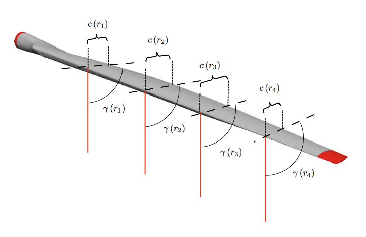
To introduce the blade forces, consider the blade depicted in Figure 6. In this model, the actual blade geometry is considered indirectly. The blades themselves are not meshed, but instead are represented by the following information:

  • \bullet

    the lift and drag curves corresponding to a given airfoil model of each blade element;

  • \bullet

    the local chord length c(r)𝑐𝑟c(r) of the blade at radius r𝑟r, which is the length of the blade element located there (see Figure 6);

  • \bullet

    the local pitch angle γ(r)𝛾𝑟\gamma(r) of the blade at radius r𝑟r; γ(r)𝛾𝑟\gamma(r) is the angle between the chord line of the blade element located at radius r𝑟r, and the rotational plane of the turbine (see Figure 7).

From this data and 𝐔relatsubscript𝐔relat{{\mathbf{U}}_{\textrm{relat}}}, two important angles are defined for each blade element (see Figure 7):

  • \bullet

    the flow angle ϕitalic-ϕ\phi, which is the angle between 𝐔relatsubscript𝐔relat{{\mathbf{U}}_{\textrm{relat}}} and the rotational plane of the turbine, and is given by

    ϕ=arctan(UxUθ+ωr),italic-ϕsubscriptU𝑥subscriptU𝜃𝜔𝑟\phi=\arctan\left(\frac{{\rm U}_{x}}{{\rm U}_{\theta}+\omega\,r}\right), (3.9)
  • \bullet

    the angle of attack α𝛼\alpha, which is the angle between 𝐔relatsubscript𝐔relat{{\mathbf{U}}_{\textrm{relat}}} and the main chord line of the blade element, and is given by

    α=ϕγ(r).𝛼italic-ϕ𝛾𝑟\alpha=\phi-\gamma(r). (3.10)
Refer to caption
Figure 6: A blade, with chord length c𝑐c and local pitch angle γ𝛾\gamma varying along its radius. Orange (solid) lines lie in the rotational plane of the turbine.
Refer to caption
Figure 7: Visualisation in the (𝐞x,𝐞θ)subscript𝐞𝑥subscript𝐞𝜃\left({\bf{e}}_{x},{\bf{e}}_{\theta}\right) plane of a blade element located at radius r𝑟r from the center of the turbine: relative velocity 𝐔relatsubscript𝐔relat{{\mathbf{U}}_{\textrm{relat}}}, rotational velocity ωr𝐞θ𝜔𝑟subscript𝐞𝜃-\omega r{\bf{e}}_{\theta}, local pitch angle γ(r)𝛾𝑟\gamma(r) and angle of attack α𝛼\alpha.

For the i𝑖i-th blade, blade element theory tells us that the total force exerted on the flow by each blade element – spanning an infinitesimal portion dr𝑑𝑟dr of the blade – is proportional to the square of the norm of 𝐔relatsubscript𝐔relat{\mathbf{U}}_{\textrm{relat}} and to the surficial area of the element, which is approximated as c(r)dr𝑐𝑟𝑑𝑟c(r)dr. The force is divided in two orthogonal components:

  • 1)

    A lift force 𝐝𝐋(i)superscript𝐝𝐋𝑖{\bf{dL}}^{(i)}, which is parallel to 𝐔relatsubscript𝐔relat{\mathbf{U}}_{\textrm{relat}}

  • 2)

    A drag force 𝐝𝐃(i)superscript𝐝𝐃𝑖{\bf{dD}}^{(i)}, which is orthogonal to 𝐔relatsubscript𝐔relat{\mathbf{U}}_{\textrm{relat}}

The expressions for the magnitudes of these forces, dL𝑑𝐿dL and dD𝑑𝐷dD, read as follows (Urelatsubscript𝑈relat{U}_{\textrm{relat}} being the magnitudes of 𝐔relatsubscript𝐔relat{\mathbf{U}}_{\textrm{relat}}):

dL(i)𝑑superscript𝐿𝑖\displaystyle dL^{(i)} =12ρUrelat2c(r)CLdr,absent12𝜌superscriptsubscript𝑈relat2𝑐𝑟subscript𝐶𝐿𝑑𝑟\displaystyle=\frac{1}{2}\rho\;{U}_{\textrm{relat}}^{2}\;c(r)\;C_{L}\;dr, (3.11)
dD(i)𝑑superscript𝐷𝑖\displaystyle dD^{(i)} =12ρUrelat2c(r)CDdr.absent12𝜌superscriptsubscript𝑈relat2𝑐𝑟subscript𝐶𝐷𝑑𝑟\displaystyle=\frac{1}{2}\rho\;{U}_{\textrm{relat}}^{2}\;c(r)\;C_{D}\;dr.

The terms CLsubscript𝐶𝐿C_{L} and CDsubscript𝐶𝐷C_{D} are called the lift coefficient and drag coefficient respectively, and are functions of the angle of attack α𝛼\alpha, as well as the local Reynolds number at the blade. These functions are determined either empirically or via numerical simulations, and are often found in the form of tabulated data. In the present work, two approaches are used to determine CLsubscript𝐶𝐿C_{L} and CDsubscript𝐶𝐷C_{D} for a given value of the angle of attack α𝛼\alpha, depending on the mill data we have:

  • -

    numerical interpolation using tabulated data giving the values of both coefficients for a range of possible values of α𝛼\alpha, corresponding to a given airfoil design at a given Reynolds number. This approach is used in Section 4.

  • -

    direct computation using analytical expressions for the dependence on the angle of attack α𝛼\alpha, corresponding to a given airfoil design at a given Reynolds number. This approach is used in Section 5.

Expressions in (3.11) depend on i𝑖i as Urelatsubscript𝑈relat{U}_{\textrm{relat}}, CLsubscript𝐶𝐿C_{L} and CDsubscript𝐶𝐷C_{D} are computed locally at each different blade position using one of the methods described above.

In the local reference frame of the turbine (see Figure 3a), the components of the differential force along 𝐞xsubscript𝐞𝑥{\bf{e}}_{x} and 𝐞θsubscript𝐞𝜃{\bf{e_{\theta}}} corresponding to the i𝑖i-th blade are, respectively:

dFx(i)𝑑superscriptsubscript𝐹𝑥𝑖\displaystyle dF_{x}^{(i)} =(dL(i)cos(ϕ)+dD(i)sin(ϕ))=12ρUrelat2c(r)(CLcos(ϕ)+CDsin(ϕ))dr,absent𝑑superscript𝐿𝑖italic-ϕ𝑑superscript𝐷𝑖italic-ϕ12𝜌superscriptsubscript𝑈relat2𝑐𝑟subscript𝐶𝐿italic-ϕsubscript𝐶𝐷italic-ϕ𝑑𝑟\displaystyle=-\left(dL^{(i)}\cos(\phi)+dD^{(i)}\sin(\phi)\right)=-\frac{1}{2}\rho\;{U}_{\textrm{relat}}^{2}\;c(r)\;\left(C_{L}\cos(\phi)+C_{D}\sin(\phi)\right)\;dr, (3.12)
dFθ(i)𝑑superscriptsubscript𝐹𝜃𝑖\displaystyle dF_{\theta}^{(i)} =dL(i)sin(ϕ)dD(i)cos(ϕ)=12ρUrelat2c(r)(CLsin(ϕ)CDcos(ϕ))dr.absent𝑑superscript𝐿𝑖italic-ϕ𝑑superscript𝐷𝑖italic-ϕ12𝜌superscriptsubscript𝑈relat2𝑐𝑟subscript𝐶𝐿italic-ϕsubscript𝐶𝐷italic-ϕ𝑑𝑟\displaystyle=dL^{(i)}\sin(\phi)-dD^{(i)}\cos(\phi)=\frac{1}{2}\rho\;{U}_{\textrm{relat}}^{2}\;c(r)\;\left(C_{L}\sin(\phi)-C_{D}\cos(\phi)\right)\;dr.

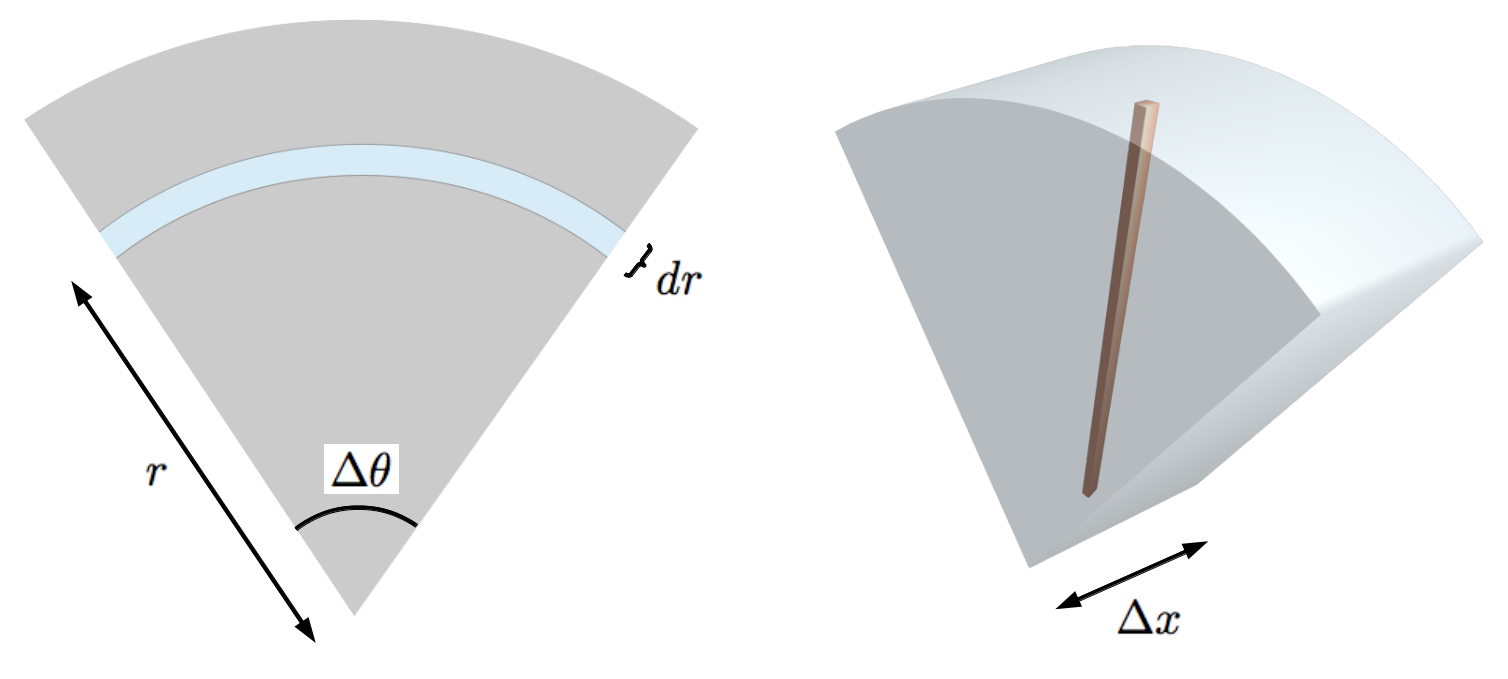
Now consider a turbine with Nbladessubscript𝑁bladesN_{\textit{blades}} blades. The aim is to use (3.12) to obtain expressions for the components of the force per unit mass along 𝐞xsubscript𝐞𝑥{\bf{e}}_{x} and 𝐞θsubscript𝐞𝜃{\bf{e}}_{\theta}, corresponding to each blade. To do this, the blade in question is expanded a distance ΔxΔ𝑥\Delta x along the axial direction, and smeared over an angular distance ΔθΔ𝜃\Delta\theta, resulting in the three dimensional region shown in Figure 8. To a blade element located at radius r𝑟r there corresponds an infinitesimal sector of volume rΔxΔθdr𝑟Δ𝑥Δ𝜃𝑑𝑟r\Delta x\Delta\theta dr and mass ρrΔxΔθdr𝜌𝑟Δ𝑥Δ𝜃𝑑𝑟\rho r\Delta x\Delta\theta dr. Dividing the expressions in (3.12) by the element sector mass, one obtains the forces per unit mass at radius r𝑟r from the center of the wind turbine:

fx(i)superscriptsubscript𝑓𝑥𝑖\displaystyle f_{x}^{(i)} =1ρrΔθΔxdFx(i)dr=12rΔθΔxUrelat2c(r)(CLcos(ϕ)+CDsin(ϕ)),absent1𝜌𝑟Δ𝜃Δ𝑥𝑑superscriptsubscript𝐹𝑥𝑖𝑑𝑟12𝑟Δ𝜃Δ𝑥superscriptsubscript𝑈relat2𝑐𝑟subscript𝐶𝐿italic-ϕsubscript𝐶𝐷italic-ϕ\displaystyle=\frac{1}{\rho r\Delta\theta\Delta x}\frac{dF_{x}^{(i)}}{dr}=-\frac{1}{2r\Delta\theta\Delta x}{U}_{\textrm{relat}}^{2}c(r)\left(C_{L}\cos(\phi)+C_{D}\sin(\phi)\right), (3.13)
fθ(i)superscriptsubscript𝑓𝜃𝑖\displaystyle f_{\theta}^{(i)} =1ρrΔθΔxdFθ(i)dr=12rΔθΔxUrelat2c(r)(CLsin(ϕ)CDcos(ϕ)).absent1𝜌𝑟Δ𝜃Δ𝑥𝑑superscriptsubscript𝐹𝜃𝑖𝑑𝑟12𝑟Δ𝜃Δ𝑥superscriptsubscript𝑈relat2𝑐𝑟subscript𝐶𝐿italic-ϕsubscript𝐶𝐷italic-ϕ\displaystyle=\frac{1}{\rho r\Delta\theta\Delta x}\frac{dF_{\theta}^{(i)}}{dr}=\frac{1}{2r\Delta\theta\Delta x}{U}_{\textrm{relat}}^{2}c(r)\left(C_{L}\sin(\phi)-C_{D}\cos(\phi)\right).
Refer to caption
Figure 8: A three dimensional sector corresponding to one blade.

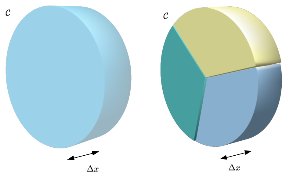
Note that expressions in (3.13) correspond to the force per unit mass of one single blade. In principle, each particle of the simulation will receive at most the force of one blade (the one corresponding to the sector where the particle is), and thus it is necessary to keep track of the positions of each blade (and the corresponding blade sector). However, if one is only interested in the global impact of the blades, it is possible to simplify the computations by selecting Δθ=2πNbladesΔ𝜃2𝜋subscript𝑁blades\Delta\theta=\frac{2\pi}{N_{\textit{blades}}}, where Nbladessubscript𝑁bladesN_{\textit{blades}} is the number of blades of the turbine. In this case, the union of all blade sectors results in the same region 𝒞bladessubscript𝒞blades\mathcal{C}_{\textit{blades}} used in section 3.1 (see Figure 9), and the blade positions become irrelevant. Expressions (3.13) then read as follows:

fxsubscript𝑓𝑥\displaystyle f_{x} =1ρ2πrΔxdFxdr=Nblades4πrΔxUrelat2c(r)(CLcos(ϕ)+CDsin(ϕ)),absent1𝜌2𝜋𝑟Δ𝑥𝑑subscript𝐹𝑥𝑑𝑟subscript𝑁blades4𝜋𝑟Δ𝑥superscriptsubscript𝑈relat2𝑐𝑟subscript𝐶𝐿italic-ϕsubscript𝐶𝐷italic-ϕ\displaystyle=\frac{1}{\rho 2\pi r\Delta x}\frac{dF_{x}}{dr}=-\frac{N_{\textit{blades}}}{4\pi r\Delta x}{U}_{\textrm{relat}}^{2}c(r)\left(C_{L}\cos(\phi)+C_{D}\sin(\phi)\right), (3.14)
fθsubscript𝑓𝜃\displaystyle f_{\theta} =1ρ2πrΔxdFθdr=Nblades4πrΔxUrelat2c(r)(CLsin(ϕ)CDcos(ϕ)).absent1𝜌2𝜋𝑟Δ𝑥𝑑subscript𝐹𝜃𝑑𝑟subscript𝑁blades4𝜋𝑟Δ𝑥superscriptsubscript𝑈relat2𝑐𝑟subscript𝐶𝐿italic-ϕsubscript𝐶𝐷italic-ϕ\displaystyle=\frac{1}{\rho 2\pi r\Delta x}\frac{dF_{\theta}}{dr}=\frac{N_{\textit{blades}}}{4\pi r\Delta x}{U}_{\textrm{relat}}^{2}c(r)\left(C_{L}\sin(\phi)-C_{D}\cos(\phi)\right).

Note that this is equivalent to summing the contributions of (3.12) for all blades, and distributing the resulting force in an annulus of mass 2πρrΔxdr2𝜋𝜌𝑟Δ𝑥𝑑𝑟2\pi\rho r\Delta xdr (or equivalently, to choosing Δθ=2πΔ𝜃2𝜋\Delta\theta=2\pi and summing the contributions of (3.13) for the Nbladessubscript𝑁bladesN_{\textit{blades}} blades). In this case, since the blades are essentially delocalised within the mill region, their contributions may be considered equal to one another, and the total force at radius r𝑟r will be given by:

dFx=i=1NbladesdFx(i)=Nblades(dLcos(ϕ)+dDsin(ϕ)),𝑑subscript𝐹𝑥superscriptsubscript𝑖1subscript𝑁blades𝑑superscriptsubscript𝐹𝑥𝑖subscript𝑁blades𝑑𝐿italic-ϕ𝑑𝐷italic-ϕ\displaystyle dF_{x}=\sum_{i=1}^{N_{\textit{blades}}}dF_{x}^{(i)}=-N_{\textit{blades}}\left(dL\cos(\phi)+dD\sin(\phi)\right), (3.15)
dFθ=i=1NbladesdFθ(i)=Nblades(dLsin(ϕ)dDcos(ϕ)).𝑑subscript𝐹𝜃superscriptsubscript𝑖1subscript𝑁blades𝑑superscriptsubscript𝐹𝜃𝑖subscript𝑁blades𝑑𝐿italic-ϕ𝑑𝐷italic-ϕ\displaystyle dF_{\theta}=\sum_{i=1}^{N_{\textit{blades}}}dF_{\theta}^{(i)}=N_{\textit{blades}}\left(dL\sin(\phi)-dD\cos(\phi)\right).

Under these assumptions, since the blade characteristics (local pitch, local chord length, lift and drag coefficients) are defined locally, and since the blade positions within 𝒞bladessubscript𝒞blades\mathcal{C}_{\textit{blades}} are indeterminate, we may use the particle positions and Lagrangian velocities (Xt,Ut)subscriptX𝑡subscriptU𝑡({\rm X}_{t},{\rm U}_{t}) to compute the angle of attack α𝛼\alpha, the local pitch angle γ𝛾\gamma and deduce all the needed information 𝐔relatsubscript𝐔relat{\mathbf{U}}_{\textrm{relat}}, c(r)𝑐𝑟c(r), CL(α)subscript𝐶𝐿𝛼C_{L}(\alpha) and CD(α)subscript𝐶𝐷𝛼C_{D}(\alpha). From (3.8), we derive the relative velocity 𝐔relatsubscript𝐔relat{\mathbf{U}}_{\textrm{relat}} from the instantaneous particle position and Lagrangian velocity (Xt,Ut)subscriptX𝑡subscriptU𝑡({\rm X}_{t},{\rm U}_{t}) by

𝐔relat(Xt,Ut)=(Ut𝐞𝐱)𝐞𝐱+((Ut𝐞θ)+ωr(Xt))𝐞θ.subscript𝐔relatsubscriptX𝑡subscriptU𝑡subscriptU𝑡subscript𝐞𝐱subscript𝐞𝐱subscriptU𝑡subscript𝐞𝜃𝜔𝑟subscriptX𝑡subscript𝐞𝜃\displaystyle{\mathbf{U}}_{\textrm{relat}}({\rm X}_{t},{\rm U}_{t})=({\rm U}_{t}\cdot{\bf{e}_{x}}){\bf{e}_{x}}+\left(({\rm U}_{t}\cdot{\bf{e}_{\theta}})+\omega\,{r}({\rm X}_{t})\right){\bf{e}_{\theta}}. (3.16)

We also compute the flow angle ϕitalic-ϕ\phi using (3.9):

ϕ(Xt,Ut)=arctan((Ut𝐞𝐱)(Ut𝐞θ)+ωr(Xt)),α(Xt,Ut)=ϕ(Xt,Ut)γ(r(Xt)).italic-ϕsubscriptX𝑡subscriptU𝑡absentsubscriptU𝑡subscript𝐞𝐱subscriptU𝑡subscript𝐞𝜃𝜔𝑟subscriptX𝑡𝛼subscriptX𝑡subscriptU𝑡absentitalic-ϕsubscriptX𝑡subscriptU𝑡𝛾𝑟subscriptX𝑡\displaystyle\begin{aligned} \phi({\rm X}_{t},{\rm U}_{t})&=\arctan\left(\frac{({\rm U}_{t}\cdot\bf{e}_{x})}{({\rm U}_{t}\cdot{\bf{e}_{\theta}})+\omega\,r({\rm X}_{t})}\right),\\ \alpha({\rm X}_{t},{\rm U}_{t})&=\phi({\rm X}_{t},{\rm U}_{t})-\gamma(r({\rm X}_{t})).\end{aligned} (3.17)

Then the force added in the Lagrangian velocity Equation (3.1) is

fx(t,Xt,Ut)subscript𝑓𝑥𝑡subscriptX𝑡subscriptU𝑡\displaystyle f_{x}(t,{\rm X}_{t},{\rm U}_{t}) =𝟙{Xt𝒞blades}Nblades4πrΔx(Urelat(Xt,Ut))2c(r(Xt))(CL(α)cos(ϕ)+CD(α)sin(ϕ))(Xt,Ut),absentsubscript1subscriptX𝑡subscript𝒞bladessubscript𝑁blades4𝜋𝑟Δ𝑥superscriptsubscript𝑈relatsubscriptX𝑡subscriptU𝑡2𝑐𝑟subscriptX𝑡subscript𝐶𝐿𝛼italic-ϕsubscript𝐶𝐷𝛼italic-ϕsubscriptX𝑡subscriptU𝑡\displaystyle=-{\mathds{1}}_{\{{\rm X}_{t}\in\mathcal{C}_{\textit{blades}}\}}\frac{N_{\textit{blades}}}{4\pi r\Delta x}\left({U}_{\textrm{relat}}({\rm X}_{t},{\rm U}_{t})\right)^{2}c(r({\rm X}_{t}))\left(C_{L}(\alpha)\cos(\phi)+C_{D}(\alpha)\sin(\phi)\right)({\rm X}_{t},{\rm U}_{t}), (3.18)
fθ(t,Xt,Ut)subscript𝑓𝜃𝑡subscriptX𝑡subscriptU𝑡\displaystyle f_{\theta}(t,{\rm X}_{t},{\rm U}_{t}) =𝟙{Xt𝒞blades}Nblades4πrΔx(Urelat(Xt,Ut))2c(r(Xt))(CL(α)sin(ϕ)CD(α)cos(ϕ))(Xt,Ut).absentsubscript1subscriptX𝑡subscript𝒞bladessubscript𝑁blades4𝜋𝑟Δ𝑥superscriptsubscript𝑈relatsubscriptX𝑡subscriptU𝑡2𝑐𝑟subscriptX𝑡subscript𝐶𝐿𝛼italic-ϕsubscript𝐶𝐷𝛼italic-ϕsubscriptX𝑡subscriptU𝑡\displaystyle={\mathds{1}}_{\{{\rm X}_{t}\in\mathcal{C}_{\textit{blades}}\}}\frac{N_{\textit{blades}}}{4\pi r\Delta x}\left({U}_{\textrm{relat}}({\rm X}_{t},{\rm U}_{t})\right)^{2}c(r({\rm X}_{t}))\left(C_{L}(\alpha)\sin(\phi)-C_{D}(\alpha)\cos(\phi)\right)({\rm X}_{t},{\rm U}_{t}).

This results in the numerical Algorithm 3.
Refer to caption
Figure 9: Left: cylinder 𝒞𝒞\mathcal{C} representing the turbine viewed by a particle. Right: decomposition of 𝒞𝒞\mathcal{C} in three blade sectors. In these figures the nacelle sector 𝒞nacellesubscript𝒞nacelle\mathcal{C}_{\textit{nacelle}} is omitted for simplicity.
Algorithm 3 -- Update the Lagrangian velocity with thrust force in the rotating actuator disc model.
  PRESTEP Compute the relevant geometrical information of the particle at time tnsubscript𝑡𝑛t_{n}, relative to the turbine:
  • the radial position r(Xtn)𝑟subscriptXsubscript𝑡𝑛r\left({\rm X}_{t_{n}}\right) of the particle (component of XtnsubscriptXsubscript𝑡𝑛{\rm X}_{t_{n}} along 𝐞rsubscript𝐞𝑟{\bf{e}}_{r})

  • the distance to the rotational plane of the turbine.

With this information, determine if XtnsubscriptXsubscript𝑡𝑛{\rm X}_{t_{n}} lies inside 𝒞bladessubscript𝒞blades\mathcal{C}_{\textit{blades}} or not.
  if Xtn𝒞bladessubscriptXsubscript𝑡𝑛subscript𝒞blades{\rm X}_{t_{n}}\in\mathcal{C}_{\textit{blades}} then
     (1) compute the tangent vector 𝐞θsubscript𝐞𝜃{\bf{e}}_{\theta} corresponding to the projection of XtnsubscriptXsubscript𝑡𝑛{\rm X}_{t_{n}} on the rotational plane of the turbine;
     (2) compute the tangential velocity of the particle, Utn(tan)superscriptsubscriptUsubscript𝑡𝑛{\rm U}_{t_{n}}^{(\tan)}; that is, its component along 𝐞θsubscript𝐞𝜃{\bf{e}}_{\theta};
     (3) compute the relative velocity 𝐔relatsubscript𝐔relat{\mathbf{U}}_{\textrm{relat}} using (3.16) and the particle velocity components at time tnsubscript𝑡𝑛t_{n}:
𝐔relat=utn𝐞x+(Utn(tan)+ωr(Xtn))𝐞θ;subscript𝐔relatsubscript𝑢subscript𝑡𝑛subscript𝐞𝑥superscriptsubscriptUsubscript𝑡𝑛𝜔𝑟subscriptXsubscript𝑡𝑛subscript𝐞𝜃{\mathbf{U}}_{\textrm{relat}}=u_{t_{n}}{\bf{e}}_{x}+\left({\rm U}_{t_{n}}^{(\tan)}+\omega\,r\left({\rm X}_{t_{n}}\right)\right){\bf{e}_{\theta}};
     (4) compute the flow angle ϕitalic-ϕ\phi using (3.17) and the particle velocity components at time tnsubscript𝑡𝑛t_{n}:
ϕ=arctan(utnUtn(tan)+ωr(Xtn));italic-ϕsubscript𝑢subscript𝑡𝑛superscriptsubscriptUsubscript𝑡𝑛𝜔𝑟subscriptXsubscript𝑡𝑛\phi=\arctan\left(\frac{u_{t_{n}}}{{\rm U}_{t_{n}}^{(\tan)}+\omega\,r\left({\rm X}_{t_{n}}\right)}\right);
     (5) compute the angle of attack α𝛼\alpha using (3.17), with the local pitch computed at the radial position of the particle:
α=ϕγ(r(Xtn));𝛼italic-ϕ𝛾𝑟subscriptXsubscript𝑡𝑛\alpha=\phi-\gamma\left(r\left({\rm X}_{t_{n}}\right)\right);
     (6) obtain the lift and drag coefficients CL(α)subscript𝐶𝐿𝛼C_{L}(\alpha) and CD(α)subscript𝐶𝐷𝛼C_{D}(\alpha) using the airfoil data;
     (7) apply the axial and tangential forces per unit mass (3.18) respectively to the particle velocity:
utn+1utn+1Nblades4πrΔx𝐔relat2c(CLcos(ϕ)+CDsin(ϕ))Δt,subscript𝑢subscript𝑡𝑛1subscript𝑢subscript𝑡𝑛1subscript𝑁blades4𝜋𝑟Δ𝑥superscriptsubscript𝐔relat2𝑐subscript𝐶𝐿italic-ϕsubscript𝐶𝐷italic-ϕΔ𝑡u_{t_{n+1}}\longmapsto u_{t_{n+1}}-\frac{N_{\textit{blades}}}{4\pi r\Delta x}{\mathbf{U}}_{\textrm{relat}}^{2}c\left(C_{L}\cos(\phi)+C_{D}\sin(\phi)\right)\Delta t,
Utn+1(tan)Utn+1(tan)+Nblades4πrΔx𝐔relat2c(CLsin(ϕ)CDcos(ϕ))Δt.superscriptsubscriptUsubscript𝑡𝑛1superscriptsubscriptUsubscript𝑡𝑛1subscript𝑁blades4𝜋𝑟Δ𝑥superscriptsubscript𝐔relat2𝑐subscript𝐶𝐿italic-ϕsubscript𝐶𝐷italic-ϕΔ𝑡{\rm U}_{t_{n+1}}^{(\tan)}\longmapsto{\rm U}_{t_{n+1}}^{(\tan)}+\frac{N_{\textit{blades}}}{4\pi r\Delta x}{\mathbf{U}}_{\textrm{relat}}^{2}c\left(C_{L}\sin(\phi)-C_{D}\cos(\phi)\right)\Delta t.
  end if

3.3 Nacelle model

In all the simulation results presented in Sections 4 and 5, we use a simple model for the turbine nacelle. As in Wu and Porté-Agel [32], the nacelle force fnacellesubscript𝑓nacellef_{\textit{nacelle}} is modeled as a permeable actuator disc, but here we adapt the model to the Lagrangian setting. The nacelle is assumed to occupy a cylinder 𝒞nacellesubscript𝒞nacelle\mathcal{C}_{\textit{nacelle}}, with frontal area Anacellesubscript𝐴nacelleA_{\textit{nacelle}} and depth ΔxΔ𝑥\Delta x (see Figure 4).

A particle (Xt,Ut)subscript𝑋𝑡subscript𝑈𝑡(X_{t},U_{t}) lying within the nacelle region is applied a force per unit mass of:

fnacelle=1Δx2anacelle1anacelle𝟙{Xt𝒞nacelle}(Ut𝐞x)2𝐞x.subscript𝑓nacelle1Δ𝑥2subscript𝑎nacelle1subscript𝑎nacellesubscript1subscriptX𝑡subscript𝒞nacellesuperscriptsubscript𝑈𝑡subscript𝐞𝑥2subscript𝐞𝑥f_{\textit{nacelle}}=-\dfrac{1}{\Delta x}\frac{2a_{\textit{nacelle}}}{1-a_{\textit{nacelle}}}{\mathds{1}}_{\{{\rm X}_{t}\in\mathcal{C}_{\textit{nacelle}}\}}(U_{t}\cdot{\bf{e}}_{x})^{2}{\bf{e}}_{x}. (3.19)

At the same time, the actuator disc models presented in Section 3.2 are modified to account for the nacelle’s presence: the relevant region for the mill forces will not be 𝒞𝒞\mathcal{C}, but instead the subregion 𝒞bladessubscript𝒞blades\mathcal{C}_{\textit{blades}} defined as (see Figure 4):

𝒞blades=𝒞𝒞nacelle.subscript𝒞blades𝒞subscript𝒞nacelle\mathcal{C}_{\textit{blades}}=\mathcal{C}\setminus\mathcal{C}_{\textit{nacelle}}. (3.20)

In this manner, only particles belonging to 𝒞bladessubscript𝒞blades\mathcal{C}_{\textit{blades}} (and not 𝒞𝒞\mathcal{C}) are applied the mill forces. Also, for the Non-Rotating Actuator Disc, the local velocity is estimated considering only particles lying inside 𝒞bladessubscript𝒞blades\mathcal{C}_{\textit{blades}}.

4 Comparison with high-resolution windtunnel measurements

In this section, the method presented above is tested against wind tunnel measurements performed at the Saint Anthony Falls Wind Tunnel, University of Minnesotta, by Chamorro and Porté-Agel [8]. The data consists of high resolution, hot-wire anemometry wind speed measurements at different downstream positions and heights. We particularly focus on three key turbulence statistics that are commonly used to characterize wind-turbine wakes: the mean and turbulence intensity profiles of the streamwise velocity, and the kinematic shear stress profile (see e.g. Wu and Porté-Agel [32]).

4.1 Experimental setup

The Saint Anthony Falls Laboratory wind tunnel consists of two main sections. The air recirculates among these main sections. Turbulence is created using a picket fence, and an adjustable ceiling height allows a zero-pressure gradient boundary layer flow to be created in the main sections. A miniature wind turbine is located in the tunnel, and sensors are placed at different upstream and downstream positions relative to the wind turbine (see [8] for details).

For the comparison between Lagrangian simulations and measurements, we used the neutrally-stratified boundary layer experiment. The main characteristics of the neutral boundary layer flow produced in the wind tunnel are summarized in Table 1a.

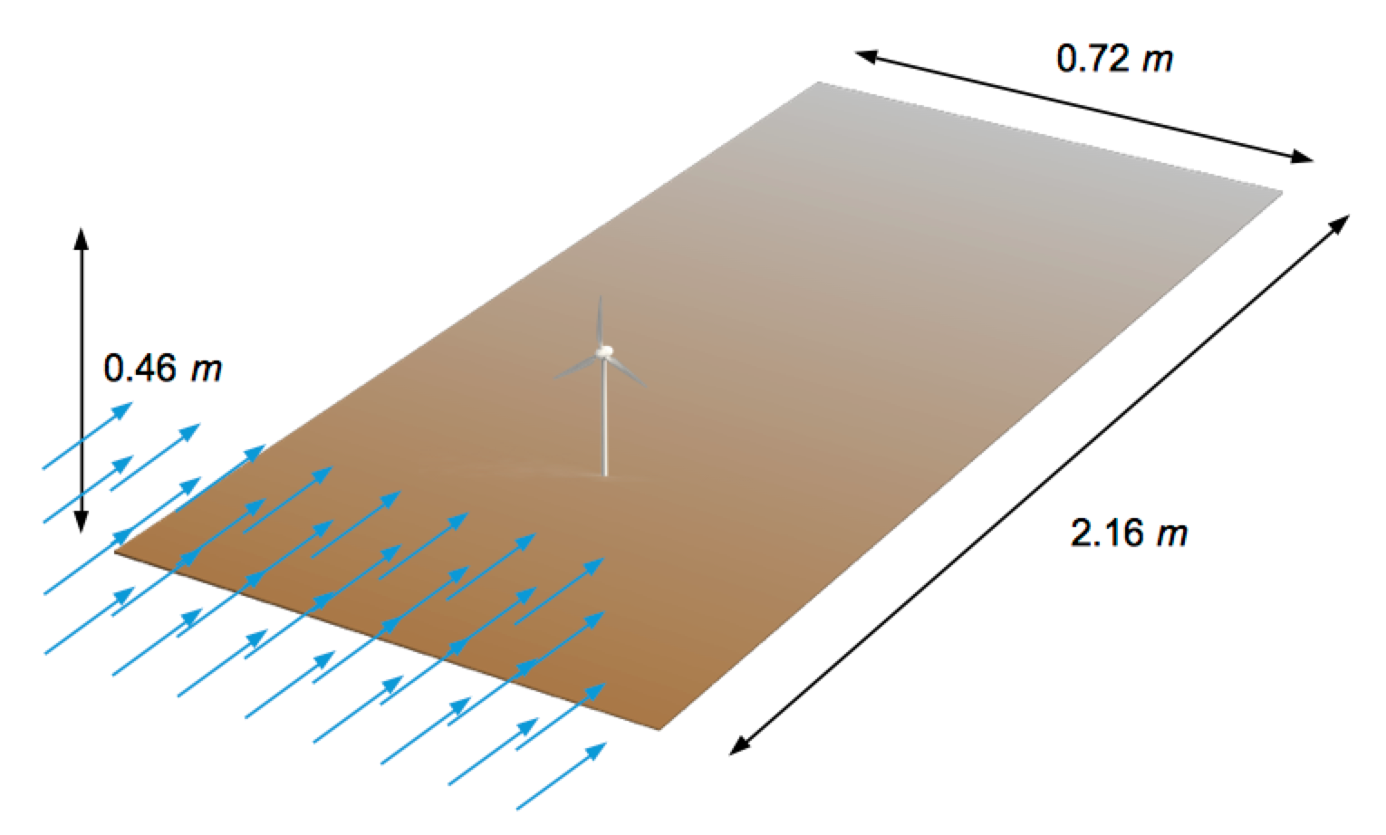
To test the implementation of mills in the stochastic Lagrangian settings presented before, a one-mill configuration reproducing the Saint Anthony Falls experiment has been used. A single mill has been placed in a rectangular domain spanning 4.32×0.72×0.464.320.720.464.32\times 0.72\times 0.46 meters in the x𝑥x, y𝑦y and z𝑧z directions, respectively (Figure 10). The mill faces atmospheric flow with a log-law profile at the inlet section, that develops moving along the x𝑥x direction. The main physical and computational parameters of the simulations are detailed in Table 1c. The miniature three-blade wind turbine is chosen so as to represent the typical dimensions and tip speed ratios of commercial wind turbines. The main parameters of the wind turbine used in the simulations are listed in Table 1d.

Boundary layer characteristics in the wind tunnel
Boundary layer depth 0.46 m
Wind speed at the top 2.8 m s1superscripts1\text{s}^{-1}
Velocity friction usubscript𝑢u_{*} 0.11 m s1superscripts1\text{s}^{-1}
Roughness length z0subscript𝑧0z_{0} 0.04 mm
(a) Main characteristics of the boundary layer flow
Model constants
Rotta constant CRsubscript𝐶𝑅C_{R} 1.8
von Karman constant κ𝜅\kappa 0.4
C2subscript𝐶2C_{2} 0.60
Cϵsubscript𝐶italic-ϵC_{\epsilon} 0.068
zmsubscript𝑧subscriptmz_{\ell_{\textrm{m}}} 0.1 m
(b) Main model physical constants
Simulation parameters
Domain size x𝑥x 2.16 m
Domain size y𝑦y 0.726 m
Domain size z𝑧z 0.42 m
96 cells in x𝑥x ΔxΔ𝑥\Delta x = 0.0225 m
33 cells in y𝑦y ΔyΔ𝑦\Delta y = 0.022 m
84 cells in z𝑧z ΔzΔ𝑧\Delta z = 0.005 m
Particles per cell 150
Final time is 30 s Time step is 0.03 s
(c) configuration of the simulations
Mill configuration
Coordinates of the hub: (0.5 0.36 0.125) m
Hub height 0.125 m
Radius 0.075 m
Nacelle radius 0.01 m
Rotational speed 112.0 rad.s1superscriptrad.s1\text{rad.s}^{-1}
Inflow factor of the nacelle anacellesubscript𝑎nacellea_{\textit{nacelle}} = 0.4
(d) parameters of the mill
Table 1: Main parameters of the wind tunnel simulations.
Refer to caption
Figure 10: Domain for the wind tunnel scale simulations.

To assess the impact of the mill in the flow, Lagrangian simulations are run with the rotating actuator disc turbine model. The mill’s position is such that the x𝑥x and y𝑦y coordinates of the hub lie at the center of one of the computational cells.

To initialize the simulations, a warm-up simulation is run first, without mill. For this warmup simulation, an inflow-outflow condition is used in the x𝑥x axis (the main direction of the wind): particles exiting the domain at the outflow boundary are reinserted at the inflow boundary with a mean velocity given by the targeted log-law444 u(z)=uκlogzz0𝑢𝑧subscript𝑢𝜅𝑧subscript𝑧0u(z)=\frac{u_{*}}{\kappa}\log\,\frac{z}{z_{0}}. plus a random velocity vector normally distributed, that renders the covariance structure taken from the cell where the particle was in the previous time step. A similar boundary condition is used in the y𝑦y axis. The results of the warmup simulation are averaged along the x𝑥x and y𝑦y axes to produce empirical profiles of all relevant statistics of the velocity field.

For the mill simulations, an inflow-outflow boundary condition is applied in the x𝑥x axis, using the empirical profile from the warmup simulation to force the inflow condition: particles exiting the domain at the outflow boundary are reinserted at the inflow one with velocities following a trivariate Gaussian distribution computed with the information of these empirical profiles. A similar strategy is used in the y𝑦y axis boundaries: particles exiting the domain through one of these boundaries are reinserted in the opposite boundary, with a new velocity following a trivariate Gaussian distribution computed with the empirical profiles.

In all simulations, the boundary conditions for the z𝑧z axis are as described in Section 2.

As in [32], we use the lift and drag data CL(α)subscript𝐶𝐿𝛼C_{L}(\alpha) and CD(α)subscript𝐶𝐷𝛼C_{D}(\alpha) provided by Blade data taken from Sunada Sakaguchi and Kawachi [31]. The chord length and twist angle of the turbine are taken from [32].

4.2 Comparison with experimental data

The results of SDM with the more complex Rotating Actuator Disc mill model is compared against experimental data obtained from Wu and Porté-Agel [32]. Three quantities are of particular interest: the streamwise component of the mean velocity field, the streamwise turbulent intensity, and the shear stress between streamwise and vertical components. As underlined in [32], du to the non-uniform (logarithmic) mean velocity profile of the incomming boundary-layer flow, the profiles of those three quantities yield non-axisymmetric distribution.

SDM simulations are showed without any time average on the SDM output produced after a total of 1000 time iterations after the warm-up phase. We show udelimited-⟨⟩𝑢{{\displaystyle{\langle}{u}\displaystyle{\rangle}}}, I𝐼I and uwdelimited-⟨⟩𝑢𝑤-{{\displaystyle{\langle}{uw}\displaystyle{\rangle}}} as they are computed at the final time step, using the second order CIC-estimator for the computation of Eulerian fields on the last 20 time steps only, to not burden the computation time.

First, we examine the streamwise component of the mean velocity. A profile comparison against experimental data at several downstream locations is shown in Figure 11. For the Rotating ADM a good agreement is seen for distances equal and higher than 5 turbine diameters, while a reasonable agreement is seen near the turbine;
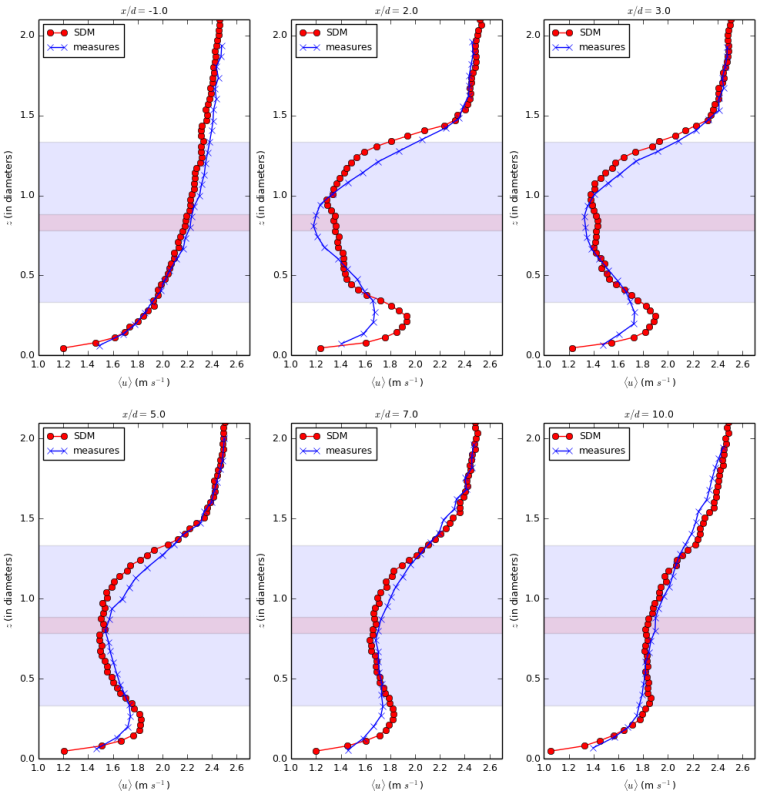
Refer to caption
Figure 11: Comparison of vertical profiles of udelimited-⟨⟩𝑢{{\displaystyle{\langle}{u}\displaystyle{\rangle}}} at different downstream positions x𝑥x from the turbine (-1, 2, 5, 7 and 10 diameters respectively). The profiles are centred to the hub y𝑦y position. The blue curve represents the wind tunnel measures, the red curve represents SDM simulation with the Rotating Actuator Disc mill model.

Secondly, the turbulence intensity I𝐼I of the stream-wise component of velocity is analyzed. Figure 12 shows the vertical turbulence intensity profiles, which are plotted at the same downstream positions as was done for udelimited-⟨⟩𝑢{{\displaystyle{\langle}{u}\displaystyle{\rangle}}}. We compute the turbulence intensity with SDM, using the same inflow mean velocity Uhubsubscript𝑈hubU_{\textrm{hub}} at the hub height than in [32]:

I=23kUhub, with Uhub=2.2 m s1.formulae-sequence𝐼23𝑘subscript𝑈hub with subscript𝑈hub2.2superscript m s1I=\frac{\sqrt{\frac{2}{3}\,{k}}}{U_{\textrm{hub}}},\quad\mbox{ with }U_{\textrm{hub}}=2.2\mbox{ m s}^{-1}.

We observe a good fit with the measures far and close to the mill, even if the turbulent intensity seems to be overestimated in the area of the nacelle (in light red) at 2 and 3 diameters of the hub.

Refer to caption
Figure 12: Comparison of vertical profiles of the turbulence intensity at different downstream positions x𝑥x from the turbine (-1, 2, 5, 7 and 10 diameters respectively). The profiles are centred to the hub y𝑦y position. The blue curve represents the wind tunnel measures, the red curve represents SDM simulation with the Rotating Actuator Disc mill model.

Also of interest is the shear stress (i.e uwdelimited-⟨⟩𝑢𝑤-{{\displaystyle{\langle}{uw}\displaystyle{\rangle}}} the covariance between x𝑥x and z𝑧z components of velocity). As before, vertical profiles are plotted for different downstream positions from the turbine. Figure 13 shows the results. Again, the fit is good but SDM seems to overestimate a little the shear stress. It is it is worth noting that the SDM computation locates the maximum of the shear stress at the top tip of the blades area (top limit of the light blue area) as expected. The same effect can be observed for the turbulent intensity.
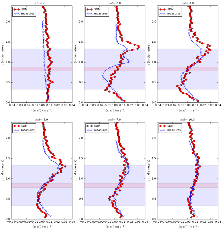
Refer to caption
Figure 13: Comparison of vertical profiles of the shear stress uwdelimited-⟨⟩superscript𝑢superscript𝑤-{{\displaystyle{\langle}{u^{\prime}w^{\prime}}\displaystyle{\rangle}}} at different downstream positions x𝑥x from the turbine (-1, 2, 5, 7 and 10 diameters respectively). The profiles are centred to the hub y𝑦y position. The blue curve represents the wind tunnel measures, the red curve represents SDM simulation with the Rotating Actuator Disc mill model.

We complement the comparison between the 2D xz𝑥𝑧xz-profiles in Figures 11 12 13, with some other directional views in Figure 14 showing in particular the winding of the streamlines passing through the turbine.
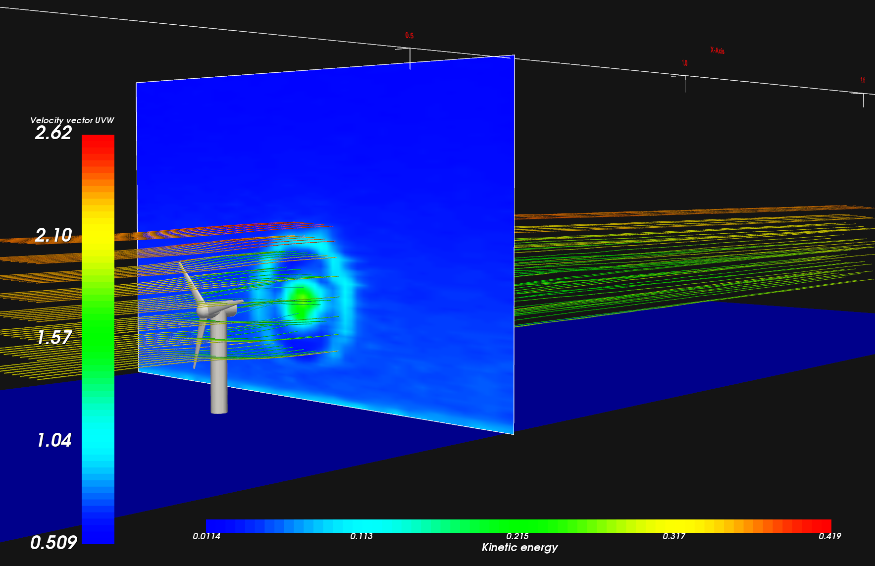
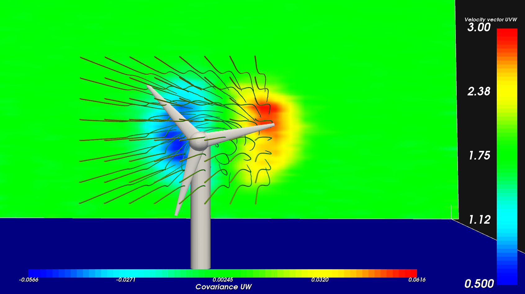
Refer to caption
Refer to caption
Figure 14: Streamlines visualization (Rotating ADM simulation), with a yz𝑦𝑧yz-contour plot of the turbulent kinetic energy circles at one diameters of the hub (left); with a yz𝑦𝑧yz-contour plot of the uwdelimited-⟨⟩superscript𝑢superscript𝑤{{\displaystyle{\langle}{u^{\prime}w^{\prime}}\displaystyle{\rangle}}} covariance at 3.5 diameters of the hub (right).

It is worth to notice that in this first Lagrangian approach for Rotating-ADM, we did not dissociate the ΔxΔ𝑥\Delta x corresponding to the thickness of the Cbladessubscript𝐶bladesC_{\textit{blades}} cylinder with the ΔxΔ𝑥\Delta x of the cell mesh. Thus, in these simulations the Cbladessubscript𝐶bladesC_{\textit{blades}} thickness is about 66% of the disk diameter. Refine this thickness independently to the cell mesh size can bring substantial improvements without additional computational cost.

Furthermore, the model of permeable disk for the nacelle can be improved (without counting the mast model that we have not put yet in our simulation). In these simulations, we introduce the corresponding force term in the velocity computation without any correction terms for the second order moments, as we did for the wall law model at the ground. There is therefore some margin of improvement for the Rotating-ADM model with SDM.

Computation time.

To produce all the results shown in this paper, we have used one 32-cores Intel Xeon CPU E5-2665 0 @ 2.40GHz computer node. The elapsed time for the 1000 iterations with 96×33×84×15096338415096\times 33\times 84\times 150 Lagrangian particles (about 40 millions of particles) is about 8 hours and 10 minutes. A new version of our code for multi-nodes computer architecture is under development.

5 Some numerical experiments at the atmospheric scale

We reproduce atmospheric turbulent condition approaching a real-size neutrally-stratified boundary layer condition, by parametrizing our simulation inspired by the numerical experiments performed in Drobinski et al. in [10] for an atmospheric neutral case. The corresponding boundary layer characteristics are summarized in Table 2b Figure 15 shows how SDM reproduces turbulence characteristics of the same order than in [10] as well as log-law profile for the velocity. In particular the anisotropic variance profiles, computed here in the whole boundary layer depth converge to zero at the top of the boundary layer. The turbulent kinetic energy goes naturally to zero at the boundary layer top and SDM fits the prescribed laminar geostrophic flow.
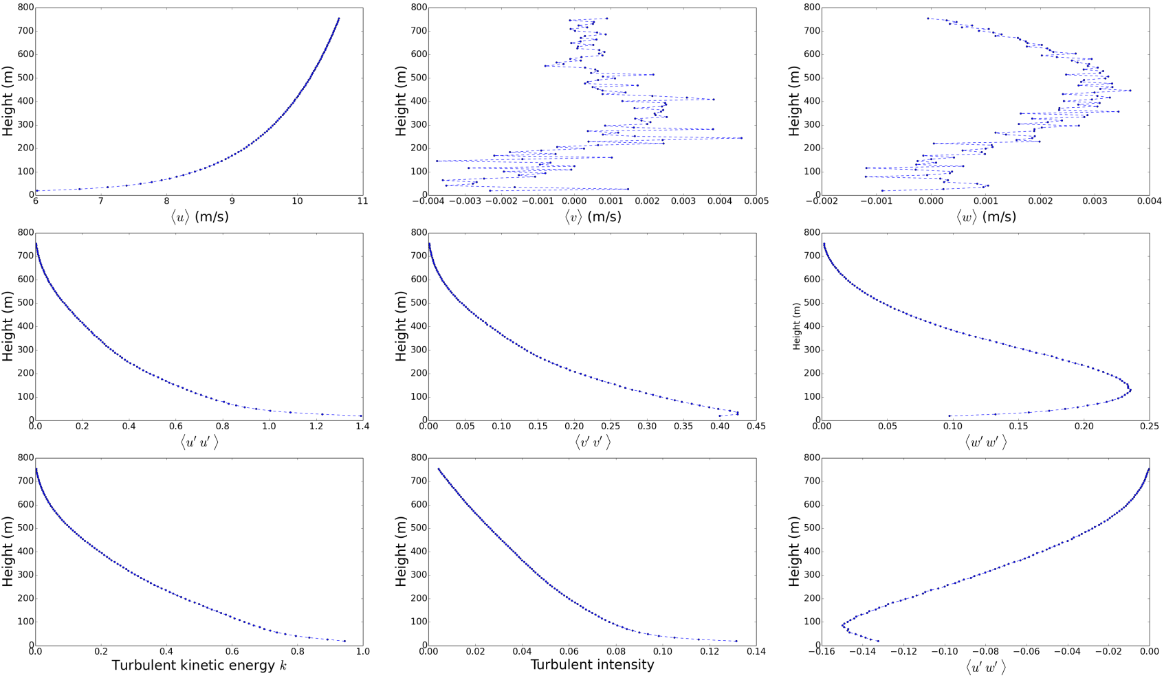
Refer to caption
Figure 15: Profiles of main turbulence charateristics computed by SDM in the whole boundary layer (averaged in the x𝑥x and y𝑦y-directions). The numerical parameters are the same than in Tables 2 exept that the computational domain height is 750 m.

5.1 Simulation setup

To test the implementation of mills in the stochastic Lagrangian settings presented before, a one-mill configuration has been used. A single mill has been placed in a rectangular domain spanning 1500×400×30015004003001500\times 400\times 300 meters in the x𝑥x, y𝑦y and z𝑧z directions, respectively (Figure 16). The mill faces atmospheric flow with a log-law profile at the inlet section, that develops moving along the x𝑥x direction. The main physical and computational parameters of the simulations are detailed in Table 2.

Boundary layer characteristics
Boundary layer depth 750 m
Wind speed at the top 10.63 m s1superscripts1\text{s}^{-1}
Velocity friction usubscript𝑢u_{*} 0.42 m s1superscripts1\text{s}^{-1}
Roughness length z0subscript𝑧0z_{0} 0.03 m
(a) Main characteristics of the boundary layer flow
Model constants
Rotta constant CRsubscript𝐶𝑅C_{R} 1.8
von Karman constant κ𝜅\kappa 0.4
C2subscript𝐶2C_{2} 0.60
Cϵsubscript𝐶italic-ϵC_{\epsilon} 0.08
zmsubscript𝑧subscriptmz_{\ell_{\textrm{m}}} 150 m
(b) Main model physical constants
Simulation parameters
Domain size x𝑥x 1488 m
Domain size y𝑦y 403 m
Domain size z𝑧z 300 m
90 cells in x𝑥x Δx=Δ𝑥absent\Delta x= 16 m
31 cells in y𝑦y Δy=Δ𝑦absent\Delta y=13 m
80 cells in z𝑧z Δz=Δ𝑧absent\Delta z= 3.75 m
Particles per cell 128
Final time is 1000 s Time step is 1.0 s
(c) configuration of the simulations
Mill configuration
Coordinates of the hub: (496.875,200,50) m
Hub height 50 m
Radius 20.5 m
Nacelle radius 4.5 m
Rotational speed 2.83 rad.s1superscriptrad.s1\text{rad.s}^{-1}
anacellesubscript𝑎nacellea_{\textit{nacelle}} for the Rotation ADM 0.38
anacellesubscript𝑎nacellea_{\textit{nacelle}} for the Non Rotation ADM 0.45
(d) parametrers of the mill
Table 2: Main parameters of the simulations at the atmospheric scale.
Refer to caption
Figure 16: Domain for the atmospheric scale simulations.

To assess the impact of the mill in the flow, simulations are run with the two turbine models presented in Section 3, namely: the non-rotating actuator disc mode (NR-ADM), and the rotating actuator disc model (R-ADM). The mill’s position is such that the x𝑥x and y𝑦y coordinates of the hub lie at the center of one of the computational cells.

To initialize the simulations, a warm-up simulation is run first, according to the same process described to initialize the wind tunnel simulation in Section 4.

For the mill simulations, an inflow-outflow boundary condition is applied in the x𝑥x axis, as described again in Section 4.

For the rotating case, a realistic wind turbine has been designed using blade data of a NTK 500/41 wind turbine (as found in [14]), together with lift and drag coefficients corresponding to a NACA 23012 airfoil at Reynolds numbers of the order of 106superscript10610^{6} (as found in Abbott and von Doenhoff [1]).

5.2 Computation of the non-rotating equivalent

For the non-rotating case, we need to specify the values of a𝑎a, CTsubscript𝐶𝑇C_{T} and Usubscript𝑈U_{\infty} (as used in Equations (3.2), (3.4), and (3.3)) so that the simulation is equivalent to the rotating actuator disc. Again, we define this equivalence by requiring the total thrust force in both cases to be the same. However, in this section we introduce an additional method to compute the required quantities, which also serves as a consistency validation of our simulations in the atmospheric case: the Blade Element Momentum method (BEM).

Compute thrust from the SDM particles

For the non-rotating (NR) actuator disc model, we compute the total thrust excluding the area Anacellesubscript𝐴nacelleA_{\textit{nacelle}} occupied by the nacelle:

FxNR=12ρ(AAnacelle)CTU2,superscriptsubscript𝐹𝑥NR12𝜌𝐴subscript𝐴nacellesubscript𝐶𝑇superscriptsubscript𝑈2F_{x}^{\text{NR}}=-\frac{1}{2}\rho(A-A_{\textit{nacelle}})C_{T}U_{\infty}^{2}, (5.1)

whereas for the rotating (R) model, the total thrust can be computed by integrating Equation (3.15) from the nacelle radius rnacellesubscript𝑟naceller_{\textit{nacelle}} to the turbine radius R𝑅R:

FxR=NbladesrnacelleR(dLdrcos(ϕ)+dDdrsin(ϕ))𝑑r.superscriptsubscript𝐹𝑥Rsubscript𝑁bladessuperscriptsubscriptsubscript𝑟nacelle𝑅𝑑𝐿𝑑𝑟italic-ϕ𝑑𝐷𝑑𝑟italic-ϕdifferential-d𝑟F_{x}^{\text{R}}=-N_{\textit{blades}}\int\limits_{r_{\textit{nacelle}}}^{R}\left(\frac{dL}{dr}\cos\left(\phi\right)+\frac{dD}{dr}\sin\left(\phi\right)\right)dr. (5.2)

The idea is then to compute Usubscript𝑈U_{\infty} and FxRsubscriptsuperscript𝐹R𝑥F^{\text{R}}_{x}, and substitute them in (5.1) to obtain CTsubscript𝐶𝑇C_{T}. The magnitude Usubscript𝑈U_{\infty} can be easily estimated as the z𝑧z-averaged value of the mean velocity Udelimited-⟨⟩U{{\displaystyle{\langle}{{\rm U}}\displaystyle{\rangle}}} at the inlet section of the domain, over the diameter of the turbine:

U=12RhRh+Ruκlog(zz0)𝑑z,subscript𝑈12𝑅superscriptsubscript𝑅𝑅subscript𝑢𝜅𝑧subscript𝑧0differential-d𝑧U_{\infty}=\frac{1}{2R}\int\limits_{h-R}^{h+R}\frac{u_{*}}{\kappa}\log\left(\frac{z}{z_{0}}\right)dz, (5.3)

To compute FxRsuperscriptsubscript𝐹𝑥RF_{x}^{\text{R}} in (5.2) from the particle information, the integrand is estimated for all particles within region 𝒞𝒞\mathcal{C}, using equations (3.18):

1ρdFxRdr=1ρ(dLdrcos(ϕ)+dDdrsin(ϕ))2πr(Xt)Δxfx(Xt,Ut).1𝜌𝑑subscriptsuperscript𝐹R𝑥𝑑𝑟1𝜌𝑑𝐿𝑑𝑟italic-ϕ𝑑𝐷𝑑𝑟italic-ϕsimilar-to-or-equals2𝜋𝑟subscriptX𝑡Δ𝑥subscript𝑓𝑥subscriptX𝑡subscriptU𝑡\frac{1}{\rho}\dfrac{dF^{\text{R}}_{x}}{dr}=\frac{1}{\rho}\left(\frac{dL}{dr}\cos\left(\phi\right)+\frac{dD}{dr}\sin\left(\phi\right)\right)\simeq-2\pi r\left({\rm X}_{t}\right)\Delta xf_{x}\left({\rm X}_{t},{\rm U}_{t}\right). (5.4)

The total thrust over ρ𝜌\rho, FxR/ρsuperscriptsubscript𝐹𝑥R𝜌F_{x}^{\text{R}}/\rho, is then computing by an estimation of the integral:

FxRρ=Rp=1Np2πr(Xtp)Δxfx(Xtp,Utp)𝟙𝒞(Xtp)p=1Np𝟙𝒞(Xtp).superscriptsubscript𝐹𝑥R𝜌𝑅superscriptsubscript𝑝1subscript𝑁𝑝2𝜋𝑟subscriptsuperscriptX𝑝𝑡Δ𝑥subscript𝑓𝑥subscriptsuperscriptX𝑝𝑡subscriptsuperscriptU𝑝𝑡subscript1𝒞subscriptsuperscriptX𝑝𝑡superscriptsubscript𝑝1subscript𝑁𝑝subscript1𝒞subscriptsuperscriptX𝑝𝑡\frac{F_{x}^{\text{R}}}{\rho}=R\;\frac{\displaystyle\sum_{p=1}^{N_{p}}2\pi\,r\left({\rm X}^{p}_{t}\right)\Delta xf_{x}\left({\rm X}^{p}_{t},{\rm U}^{p}_{t}\right){\mathds{1}}_{\mathcal{C}}\left({\rm X}^{p}_{t}\right)}{\displaystyle\sum_{p=1}^{N_{p}}{\mathds{1}}_{\mathcal{C}}\left({\rm X}^{p}_{t}\right)}. (5.5)

Compute thrust with BEM

A complete description of BEM theory can be found in [14] or [18]. It stems from the combination of two different analyses of the turbine performance facing a steady-state, uniform, radially symmetric flow:

  • (1)

    a linear and angular momentum balance in thin, radially distributed, annular stream tubes passing through the turbine swept area at different radii;

  • (2)

    a blade element analysis of the turbine.

The first of these analyses assumes that the relative velocity decrease from the far upstream region to the disc region depends on the radial position, so that a𝑎a now varies with r𝑟r:

a(r)=UUD(r)U.𝑎𝑟subscript𝑈subscript𝑈𝐷𝑟subscript𝑈a(r)=\frac{U_{\infty}-U_{D}(r)}{U_{\infty}}. (5.6)

It is also assumed that the flow gains angular momentum, related to the rotational speed of the turbine. The angular speed Uθsubscript𝑈𝜃U_{\theta} at radius r𝑟r at the disc is controlled by an additional function a(r)superscript𝑎𝑟a^{\prime}(r):

Uθ(r)=a(r)ωr,subscript𝑈𝜃𝑟superscript𝑎𝑟𝜔𝑟U_{\theta}(r)=a^{\prime}(r)\omega r, (5.7)

where ω𝜔\omega is the angular speed of the turbine. The following expressions are then found for the differential forces in directions 𝐞xsubscript𝐞𝑥{\bf{e}}_{x} and 𝐞θsubscript𝐞𝜃{\bf{e}}_{\theta}, at an annulus located at radius r𝑟r from the turbine’s center (see [18] or [14] for details):

dFx(r)𝑑subscript𝐹𝑥𝑟\displaystyle dF_{x}(r) =4πρra(r)(1a(r))U2dr,absent4𝜋𝜌𝑟𝑎𝑟1𝑎𝑟superscriptsubscript𝑈2𝑑𝑟\displaystyle=-4\pi\rho ra(r)(1-a(r))U_{\infty}^{2}dr, (5.8)
dFθ(r)𝑑subscript𝐹𝜃𝑟\displaystyle dF_{\theta}(r) =4πρωa(r)(1a(r))Ur2dr.absent4𝜋𝜌𝜔superscript𝑎𝑟1𝑎𝑟subscript𝑈superscript𝑟2𝑑𝑟\displaystyle=4\pi\rho\omega a^{\prime}(r)(1-a(r))U_{\infty}r^{2}dr. (5.9)

Given the assumption of radially symmetric flow made by BEM, in this analysis 𝐔relatsubscript𝐔relat{\mathbf{U}}_{\textrm{relat}} and the angle ϕitalic-ϕ\phi are functions of r𝑟r only. In terms of a(r)𝑎𝑟a(r) and a(r)superscript𝑎𝑟a^{\prime}(r), expressions (3.8) and (3.9) are simplified to:

𝐔relat(r)=(1a(r))U𝐞x+(1+a(r))ωr𝐞θ,subscript𝐔relat𝑟1𝑎𝑟subscript𝑈subscript𝐞𝑥1superscript𝑎𝑟𝜔𝑟subscript𝐞𝜃{\mathbf{U}}_{\textrm{relat}}(r)=(1-a(r))U_{\infty}{\bf{e}}_{x}+(1+a^{\prime}(r))\omega r{\bf{e}}_{\theta}, (5.10)
ϕ(r)=arctan((1a(r))U(1+a(r))ωr).italic-ϕ𝑟1𝑎𝑟subscript𝑈1superscript𝑎𝑟𝜔𝑟\phi(r)=\arctan\left(\frac{(1-a(r))U_{\infty}}{(1+a^{\prime}(r))\omega r}\right). (5.11)

On the other hand, a pure blade element analysis like the one presented in Section 3.2 yields the following expressions for the same quantities:

dFx(r)𝑑subscript𝐹𝑥𝑟\displaystyle dF_{x}(r) =12NbladescρUrelat2(r)(CLcos(ϕ(r))+CDsin(ϕ(r)))dr,absent12subscript𝑁blades𝑐𝜌superscriptsubscript𝑈relat2𝑟subscript𝐶𝐿italic-ϕ𝑟subscript𝐶𝐷italic-ϕ𝑟𝑑𝑟\displaystyle=-\frac{1}{2}N_{\textit{blades}}c\rho\;{U}_{\textrm{relat}}^{2}(r)(C_{L}\cos(\phi(r))+C_{D}\sin(\phi(r)))dr, (5.12)
dFθ(r)𝑑subscript𝐹𝜃𝑟\displaystyle dF_{\theta}(r) =12NbladescρUrelat2(r)(CLsin(ϕ(r))CDcos(ϕ(r)))dr.absent12subscript𝑁blades𝑐𝜌superscriptsubscript𝑈relat2𝑟subscript𝐶𝐿italic-ϕ𝑟subscript𝐶𝐷italic-ϕ𝑟𝑑𝑟\displaystyle=\frac{1}{2}N_{\textit{blades}}c\rho\;{U}_{\textrm{relat}}^{2}(r)(C_{L}\sin(\phi(r))-C_{D}\cos(\phi(r)))dr. (5.13)

In BEM, the rotor is discretized in a finite number of blade elements. For a set of radial positions and given values of Usubscript𝑈U_{\infty} and ω𝜔\omega, the values of a𝑎a and asuperscript𝑎a^{\prime}, the flow angle ϕitalic-ϕ\phi and the relative velocity magnitude Urelatsubscript𝑈relat{U}_{\textrm{relat}} are computed for each blade element separately, by equating (5.8) with (5.12) and (5.9) with (5.13) and using an iterative procedure (see [14] for a detailed description of the algorithm). The procedure delivers the values of Urelat(r)subscript𝑈relat𝑟{U}_{\textrm{relat}}(r), ϕ(r)italic-ϕ𝑟\phi(r), a(r)𝑎𝑟a(r) and a(r)superscript𝑎𝑟a^{\prime}(r).

Two Non-Rotating equivalent models are obtained:

one with the computation of the thrust according to (5.5), and the other using the BEM method described above. The corresponding estimated values for the thrust coefficient are reported in Table  3. The a𝑎a values produced par the two methods are so close that the plotting of the corresponding simulation profiles (as those in Figures 17 and 19) are completely indistinguishable. This first comparison validates the thrust equivalence computation with the SDM particles, but as we will see in the next section, at least with this value of a𝑎a, the NR-ADM underestimates the three main characteristic that we analyze in the flow, udelimited-⟨⟩𝑢{{\displaystyle{\langle}{u}\displaystyle{\rangle}}}, uudelimited-⟨⟩superscript𝑢superscript𝑢{{\displaystyle{\langle}{u^{\prime}u^{\prime}}\displaystyle{\rangle}}} and uwdelimited-⟨⟩superscript𝑢superscript𝑤{{\displaystyle{\langle}{u^{\prime}w^{\prime}}\displaystyle{\rangle}}}.

In addition to the assumptions of homogeneity and symmetry of the wind fields that are not well respected in our case, the thrust computation methods described above may be sensitive to the blade geometry discretization parameter (in our data dr=𝑑𝑟absentdr=1m) for the BEM-based method, to the ΔxΔ𝑥\Delta x parameter for the density estimator, in (5.5) for the SDM particles-based method.

Equivalent non rotating actuator disc parameter estimations
Method FxR/ρsubscriptsuperscript𝐹R𝑥𝜌\displaystyle F^{\text{R}}_{x}/\rho  (Nbladesm3/kgsubscript𝑁bladessuperscriptm3kgN_{\textit{blades}}\text{m}^{3}/\text{kg}) a𝑎{a} CTsubscript𝐶𝑇C_{T}
SDM Particle computation 28680.55 0.2081584 0.659314
BEM computation 27863.06 0.2034322 0.648190
Table 3: Estimation of the equivalent non-rotating actuator disc for our mill configuration.

5.3 Numerical experiments, comparison between rotating and non-rotating actuator disc methods

It is interesting and useful to analyze the differences between results obtained with the simple Non-Rotating model and the more complex Rotating model, and to determine to which extent they give a similar development of the turbine wake. In particular, as can be seen in the simulations of Wu and Porté-Agel [32], one would expect an under-prediction of the speed deficit near the turbine for the non-rotating case, while both models should yield similar results far downstream from the turbine. This and other effects are studied hereafter.

To begin with, mean velocity contour plots along the stream-wise direction are shown for both models in Figure 17.

Refer to captionRefer to caption
Figure 17: Comparison of xz𝑥𝑧xz cross sections of udelimited-⟨⟩𝑢{{\displaystyle{\langle}{u}\displaystyle{\rangle}}}: Rotating Actuator Disc (top), Non-Rotating Actuator Disc with a𝑎a estimated from thrust equivalence (bottom).

These plots show that rotation and non-uniform loading have a clear impact in the turbine wake. This is confirmed by the mean velocity profiles at different downstream positions, as shown in Figure 18. As expected the Rotating AD model and the Non-Rotating AD model present substantial differences, as already observed in the LES framework in [32]. The mean velocity component udelimited-⟨⟩𝑢{{\displaystyle{\langle}{u}\displaystyle{\rangle}}} is underestimates in the disk area (blades area corresponds to the light blue zone, and the nacelle area corresponds to the light red zone in the plots).
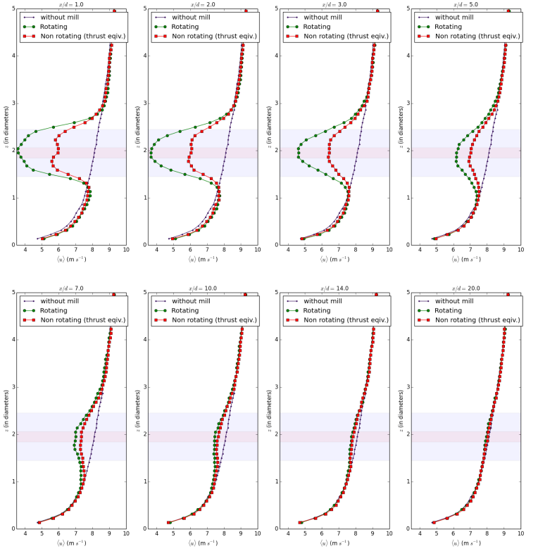
Refer to caption
Figure 18: udelimited-⟨⟩𝑢{{\displaystyle{\langle}{u}\displaystyle{\rangle}}} profiles at different downstream positions from the turbine.

Secondly, the variance of the stream-wise component of velocity uudelimited-⟨⟩superscript𝑢superscript𝑢{{\displaystyle{\langle}{u^{\prime}u^{\prime}}\displaystyle{\rangle}}} is analyzed. Figure 19 shows contour plots taken at the middle of the xz𝑥𝑧xz plane, for both simulations. It is noteworthy that the variance near the turbine is much higher for the rotating actuator disc simulation, although far from the turbine the differences begin to fade. It is also interesting that in Rotating AMD case the highest amount of variance is generated atop the turbine, while for the Non-Rotating AMD the variance at the hub is uniformly strong along the turbine disc, and not just at the tip top. We can obverse the impact of this variance anomaly that propagates in the particles environment behind the mill to the left and top. Knowing this, a remedy may consist to impose the values of the second order moments at the left boundary side from the warmup simulation to overcome this weird propagation of the variance.

The same behavior can be seen in the vertical variance profiles, which are plotted at the same downstream positions as was done for udelimited-⟨⟩𝑢{{\displaystyle{\langle}{u}\displaystyle{\rangle}}} (see Figure 20). At one diameter from the turbine, we can observe the overestimation of uudelimited-⟨⟩superscript𝑢superscript𝑢{{\displaystyle{\langle}{u^{\prime}u^{\prime}}\displaystyle{\rangle}}} for the NR-ADM (in red), in particular in the nacelle area. A best estimate of anacellesubscript𝑎nacellea_{\textit{nacelle}} could therefore contribute to reduce this variance anomaly.

Refer to captionRefer to caption
Figure 19: Comparison of xz𝑥𝑧xz cross section of variance uudelimited-⟨⟩superscript𝑢superscript𝑢{{\displaystyle{\langle}{u^{\prime}u^{\prime}}\displaystyle{\rangle}}} along x𝑥x: Rotating Actuator Ddisc (top), Non-Rotating Actuator Disc with a𝑎a estimated from thrust equivalence (bottom).
Refer to caption
Figure 20: uudelimited-⟨⟩superscript𝑢superscript𝑢{{\displaystyle{\langle}{u^{\prime}u^{\prime}}\displaystyle{\rangle}}} profiles at different downstream positions from the turbine.

Also of interest is the covariance between x𝑥x and z𝑧z components of velocity. As before, to compare both simulations, xz𝑥𝑧xz contour plots are taken at the middle of the y𝑦y axis, and vertical profiles are plotted for different downstream positions from the turbine. Again, the rotating model produces stronger values of covariance near the turbine with respect to the non-rotating model, while both tend to equalize as one moves to the far downstream section. Figure 22 shows the results.
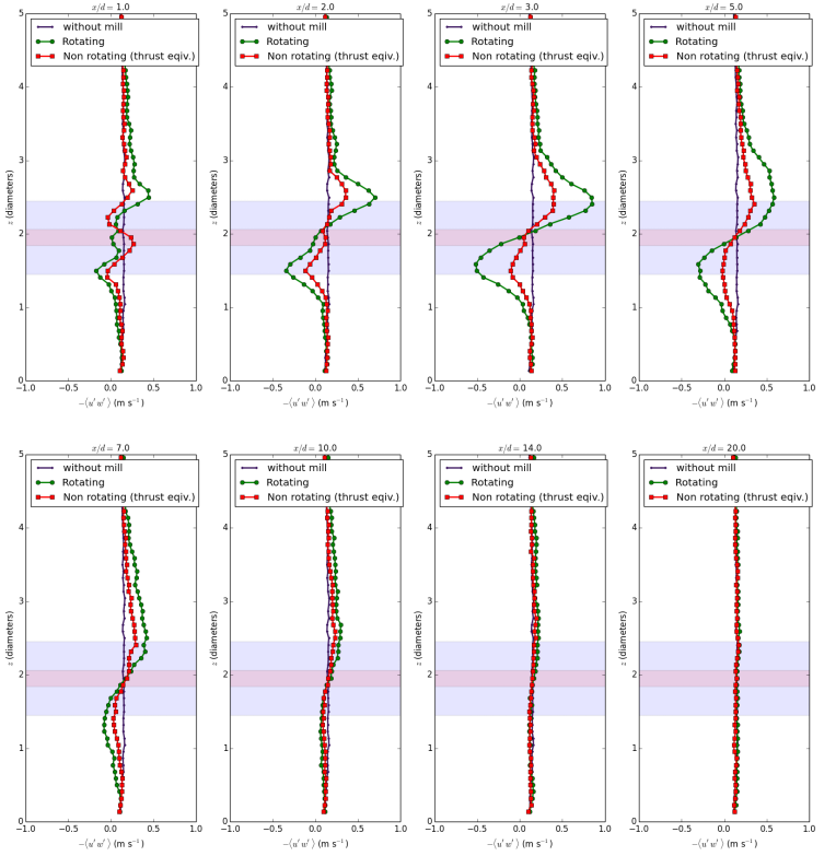
Refer to caption
Figure 21: uwdelimited-⟨⟩superscript𝑢superscript𝑤{{\displaystyle{\langle}{u^{\prime}w^{\prime}}\displaystyle{\rangle}}} profiles at different downstream positions from the turbine.

Figure 21 gives some yz𝑦𝑧yz-cross sections of the covariance at the same x𝑥x-distance to the turbine. The spacial structures of the covariances are similar, but the level of the shear is about three times smaller for the NR-ADM at 3.5 diameters from the turbine.
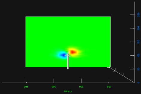
Refer to caption
Refer to caption
Refer to caption
Refer to caption
Figure 22: Comparison of the yz𝑦𝑧yz cross section of covariance uwdelimited-⟨⟩superscript𝑢superscript𝑤{{\displaystyle{\langle}{u^{\prime}w^{\prime}}\displaystyle{\rangle}}}: Rotating Actuator Disc (left), Non-Rotating Actuator Disc with a𝑎a estimated from thrust equivalence (right).

5.4 Probability distribution functions of the streamwise velocity

One of the main advantages of the stochastic downscaling method presented in Section 2 is that it allows access to the instantaneous probability distribution functions of the wind velocity field at each time and position. In the case of mill simulations, this information may be used for various purposes. Contrary to deterministic methods, the stochastic methodology used here estimates the PDFs of the velocity field in just one simulation, directly by sampling the particle properties in the same way the various statistics presented before are estimated. Plus, no time or spatial averaging is required, and it is possible to see how the PDF varies along the wake of a turbine.

In this section, we present histograms that estimate the PDF of the streamwise velocity component u=u+u𝑢delimited-⟨⟩𝑢superscript𝑢u={{\displaystyle{\langle}{u}\displaystyle{\rangle}}}+u^{\prime}, corresponding to several points before and after the wind turbine, located at the middle of the y𝑦y axis and at hub height. To obtain each histogram, we discretise velocity space and sample the particle information of all cells in the neighborhood of the point of interest.
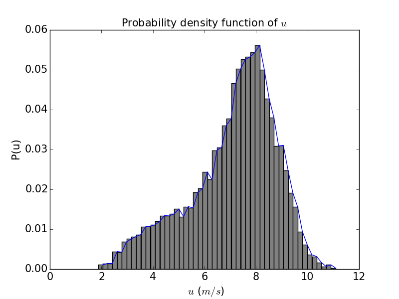
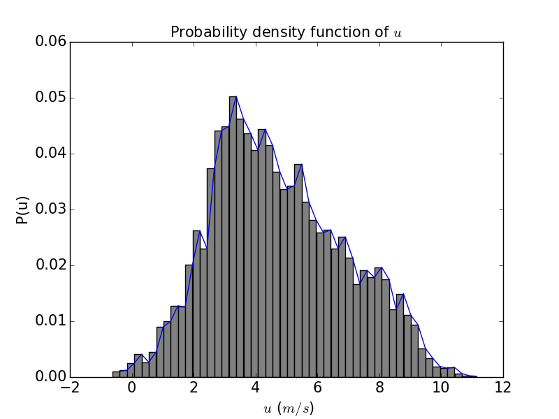
Refer to caption
(a) -1 diameters from turbine
Refer to caption
(b) 2 diameters from turbine
Refer to caption
(c) 3 diameters from turbine
Refer to caption
(d) 4 diameters from turbine
Refer to caption
(e) 5 diameters from turbine
Refer to caption
(f) 7 diameters from turbine
Figure 23: Local distribution of velocity component u=u+u𝑢delimited-⟨⟩𝑢superscript𝑢u={{\displaystyle{\langle}{u}\displaystyle{\rangle}}}+u^{\prime} at different positions of the x𝑥x axis.

As can be seen in Figure 23, the distribution of u𝑢u is fairly non-symmetric at 11-1 diameter before the turbine (where the flow has not yet felt its presence) with a peak around 8 m s-1, moving to around 3 m s-1 in the near turbine wake, progressively recovering to the 11-1 diameter distribution as one moves downstream from the turbine, and showing a bimodal distribution transition at 3 and 4 diameters from the turbine.

6 Conclusions

In recent years, wind energy has seen an important growth worldwide, and the construction and operation of large wind farms necessitates a better understanding of the flow inside and through them in realistic and dynamic atmospheric conditions. In the present study, actuator disc methods have been coupled with the SDM solver [4], which uses a probability distribution function (PDF) approach to turbulent flow simulation based on stochastic Lagrangian models. The result is an innovative methodology to simulate wind turbines and wind farms operating in atmospheric boundary layer flow. It has been shown that the particle setting of SDM is fit for mill simulations, providing qualitatively consistent estimations of the mill forces and wake properties. Plus, the PDF framework coupled with actuator disc methods allows one to obtain an estimation of the wind variability in the wake of a wind turbine, something which - to the best knowledge of the authors - has never been accomplished before.

The present work is part of a larger project, which seeks to simulate large wind farms with complex topography using the SDM solver. Moreover as a downscaling method, SDM aims to be coupled with dynamic boundary conditions coming typically from mesoscale meteorological solvers. Here, the intent has been to present the methodology, as well as to give a preliminary validation analysis with respect to measurements and a comparison of the different models available, using simple attaptation of actuator disc models and just one turbine. Future stages of the project will produce: (1) a wind farm simulation using dynamical downscaled boundary conditions coming from a coarse meteorological solver; (2) simulations with complex topography; and (3) implementation of more complex models for the blade forces in the SDM framework.

Regarding this last point, we would like to conclude showing some of our ongoing work concerning individual blade visualizations, using the methodology presented in Section 3.2. In particular, it is possible - by modifying the shape of the blade sectors - to obtain estimations of more involved 3D quantities than the ones presented here, such as the vorticity structures generated behind an individual mill. As proof of concept, Figure 24 shows a visualization of such structures for the same turbine presented in Section 5, but using a finer discretization and a smaller domain. Future stages of our project will perfect these preliminary simulations, by introducing more complex models than the Lagrangian actuator disc models presented in this work.
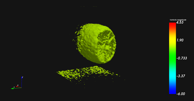
Refer to caption
Figure 24: Iso-surfaces of the x𝑥x component of vorticity behind a wind turbine.

Acknowledgments

The authors thank Philippe Drobinski for very fruitful discussions related to modeling aspects of the atmospheric boundary layer.

Appendix A Appendix

On the partial exponential Euler scheme for partially linear SDEs

A part of the drift of the fluid-particle velocity equation (2.1b) is a linear term of the form

G(t,Xt)(UtU(t,Xt)).𝐺𝑡subscriptX𝑡subscriptU𝑡delimited-⟨⟩U𝑡subscriptX𝑡-G(t,{\rm X}_{t})({\rm U}_{t}-{{\displaystyle{\langle}{{\rm U}}\displaystyle{\rangle}}}(t,{\rm X}_{t})).

It means that during a time step ΔtΔ𝑡\Delta t, each component of the velocity behaves like a one-dimensional Ornstein-Uhlenbeck process of generic form: given Ztsubscript𝑍𝑡Z_{t},

dZs=(α(Zsm)+β)ds+σdWs,for s[t,t+Δt],formulae-sequence𝑑subscript𝑍𝑠𝛼subscript𝑍𝑠𝑚𝛽𝑑𝑠𝜎𝑑subscript𝑊𝑠for 𝑠𝑡𝑡Δ𝑡\displaystyle dZ_{s}=\left(\alpha(Z_{s}-m)+\beta\right)ds+\sigma dW_{s},~{}\mbox{for }s\in[t,t+\Delta t], (A.1)

where here we assume that α0𝛼0\alpha\leq 0, σ𝜎\sigma, m𝑚m and β𝛽\beta are constants, or coefficients values frozen at the time t𝑡t. Typically, from the tensor terms G(t,Xt)𝐺𝑡subscriptX𝑡G(t,{\rm X}_{t}), we put in α𝛼\alpha only the diagonal terms, while extra diagonal terms are included in β𝛽\beta.

To simplify the presentation, assume that we work coordinate by coordinate, and that Brownian motion W𝑊W and all the coefficients are valued in \mathbb{R}. Such linear SDE (A.1) has an explicit solution Z𝑍Z valued in \mathbb{R} and given by

Zt+Δtsubscript𝑍𝑡Δ𝑡\displaystyle Z_{t+\Delta t} =eαΔtZt+(mβα)×(1eαΔt)+σeαΔttt+Δteαr𝑑Wr.absentsuperscripte𝛼Δ𝑡subscript𝑍𝑡𝑚𝛽𝛼1superscripte𝛼Δ𝑡𝜎superscripte𝛼Δ𝑡superscriptsubscript𝑡𝑡Δ𝑡superscripte𝛼𝑟differential-dsubscript𝑊𝑟\displaystyle={\rm e}^{\alpha\Delta t}Z_{t}+\left(m-\frac{\beta}{\alpha}\right)\times\left(1-{\rm e}^{\alpha\;\Delta t}\right)+\sigma{\rm e}^{\alpha\;\Delta t}\int_{t}^{t+\Delta t}{\rm e}^{-\alpha r}dW_{r}.

It is classical to notice that σeαttt+Δteαr𝑑Wr𝜎superscripte𝛼𝑡superscriptsubscript𝑡𝑡Δ𝑡superscripte𝛼𝑟differential-dsubscript𝑊𝑟\sigma{\rm e}^{\alpha\;t}\int_{t}^{t+\Delta t}{\rm e}^{-\alpha r}dW_{r} is normally distributed with Gaussian law 𝒩(0,γ2)𝒩0superscript𝛾2{\mathscr{N}}(0,\gamma^{2}), where

γ2=σ2e2αΔt0Δte2αr𝑑r=σ2α[e2αΔt1].superscript𝛾2superscript𝜎2superscripte2𝛼Δ𝑡superscriptsubscript0Δ𝑡superscripte2𝛼𝑟differential-d𝑟𝜎2𝛼delimited-[]superscripte2𝛼Δ𝑡1\gamma^{2}=\sigma^{2}{\rm e}^{2\alpha\Delta t}\int_{0}^{\Delta t}{\rm e}^{-2\alpha r}dr=\frac{\sigma}{2\alpha}\left[{\rm e}^{2\alpha\Delta t}-1\right].

We thus have the following exact simulation formula for Ztn+1subscript𝑍subscript𝑡𝑛1Z_{t_{n+1}}, given Ztnsubscript𝑍subscript𝑡𝑛Z_{t_{n}}

Ztn+1=eαΔt(Ztnm+βα)+(mβα)+σ1exp(2αΔt)(2α)ηn,subscript𝑍subscript𝑡𝑛1superscripte𝛼Δ𝑡subscript𝑍subscript𝑡𝑛𝑚𝛽𝛼𝑚𝛽𝛼𝜎12𝛼Δ𝑡2𝛼subscript𝜂𝑛\displaystyle Z_{t_{n+1}}={\rm e}^{\alpha\Delta t}\left(Z_{t_{n}}-m+\frac{\beta}{\alpha}\right)+\left(m-\frac{\beta}{\alpha}\right)+\sigma\frac{\sqrt{1-\exp(2\alpha\Delta t)}}{\sqrt{(-2\alpha)}}\eta_{n},

where (ηn)subscript𝜂𝑛(\eta_{n}) is a sequence of independent 𝒩(0,1)𝒩01{\mathscr{N}}(0,1)-identically distributed random variables. This procedure delivers a discrete time random process with the exact law of the solution of (A.1), as long as m𝑚m, α𝛼\alpha, β𝛽\beta and σ𝜎\sigma are constant. In the situation of Equation (2.1b), all those parameters may correspond to frozen coefficients αn,σn,mn,βnsubscript𝛼𝑛subscript𝜎𝑛subscript𝑚𝑛subscript𝛽𝑛\alpha_{n},\sigma_{n},m_{n},\beta_{n} during the integration step [tn,tn+Δt]subscript𝑡𝑛subscript𝑡𝑛Δ𝑡[t_{n},t_{n}+\Delta t], and the exponential Euler scheme below becomes an approximation procedure:

Z¯tn+1=eαnΔt(Z¯tnmn+βnαn)+(mnβnαn)+σn1exp(2αnΔt)(2αn)ηn.subscript¯𝑍subscript𝑡𝑛1superscriptesubscript𝛼𝑛Δ𝑡subscript¯𝑍subscript𝑡𝑛subscript𝑚𝑛subscript𝛽𝑛subscript𝛼𝑛subscript𝑚𝑛subscript𝛽𝑛subscript𝛼𝑛subscript𝜎𝑛12subscript𝛼𝑛Δ𝑡2subscript𝛼𝑛subscript𝜂𝑛\displaystyle\overline{Z}_{t_{n+1}}={\rm e}^{\alpha_{n}\Delta t}\left(\overline{Z}_{t_{n}}-m_{n}+\frac{\beta_{n}}{\alpha_{n}}\right)+\left(m_{n}-\frac{\beta_{n}}{\alpha_{n}}\right)+\sigma_{n}\frac{\sqrt{1-\exp(2\alpha_{n}\Delta t)}}{\sqrt{(-2\alpha_{n})}}\eta_{n}. (A.2)

Such exponential scheme strategy was previously considered in the context of Lagrangian two-phase flow modeling by Minier, Peirano and Chibbaro [22], who numerically analyses the ability of such method to be insensitive to some limit value of the time scale 1αn1subscript𝛼𝑛\tfrac{1}{\alpha_{n}}.

Here, our concern slightly differ. To be precise, the main advantage of the partial exponential Euler scheme to the classical Euler scheme, defined as (with the same notation for coefficients)

Z¯¯tn+1=Z¯¯tn+αn(Z¯¯tnmn)Δt+σnΔtηn,subscript¯¯𝑍subscript𝑡𝑛1subscript¯¯𝑍subscript𝑡𝑛subscript𝛼𝑛subscript¯¯𝑍subscript𝑡𝑛subscript𝑚𝑛Δ𝑡subscript𝜎𝑛Δ𝑡subscript𝜂𝑛\displaystyle\overline{\overline{Z}}_{t_{n+1}}=\overline{\overline{Z}}_{t_{n}}+\alpha_{n}(\overline{\overline{Z}}_{t_{n}}-m_{n})\Delta t+\sigma_{n}\sqrt{\Delta t}\eta_{n},

arises from the fact that the rate of strong convergence of the exponential scheme depends only on the time variation of the map tα(t)maps-to𝑡𝛼𝑡t\mapsto\alpha(t) withing its Lipschitz or Hölder regularity parameters, but does not depend directly on the values of αnsubscript𝛼𝑛\alpha_{n}. This is not true for the classical Euler scheme (see the computation below).

Concerning the time discretisation part, the convergence of our numerical scheme, described in section 2.2, is mainly driven by the notion of the weak convergence:

|𝔼f(ZT)𝔼f(Z¯T)|0,when Δt0,formulae-sequence𝔼𝑓subscript𝑍𝑇𝔼𝑓subscript¯𝑍𝑇0when Δ𝑡0|\displaystyle{\mathbb{E}}f(Z_{T})-\displaystyle{\mathbb{E}}f(\overline{Z}_{T})|\longrightarrow 0,\mbox{when }\Delta t\rightarrow 0,

given a set on test function f𝑓f. But the notion of strong convergence of a p𝑝p-th moment approximation:

(𝔼[|ZTZ¯T|p])1/p0,when Δt0formulae-sequencesuperscript𝔼delimited-[]superscriptsubscript𝑍𝑇subscript¯𝑍𝑇𝑝1𝑝0when Δ𝑡0\left(\displaystyle{\mathbb{E}}[|Z_{T}-\overline{Z}_{T}|^{p}]\right)^{1/p}\longrightarrow 0,\mbox{when }\Delta t\rightarrow 0

plays also an important role when one mix a SDE time discretisation scheme with a Monte Carlo procedure. Indeed, a particular attention should be paid to the upper-bound of the overall variance of the error: when

𝔼f(ZT)is approximated by 1Ni=1Nf(Z¯T(i)),𝔼𝑓subscript𝑍𝑇is approximated by 1𝑁superscriptsubscript𝑖1𝑁𝑓superscriptsubscript¯𝑍𝑇𝑖\displaystyle{\mathbb{E}}f(Z_{T})~{}\mbox{is approximated by }~{}\frac{1}{N}\sum_{i=1}^{N}f(\overline{Z}_{T}^{(i)}),

classical error analysis decomposes the error in the time discretisation error part (bias bound) and the mean square Monte Carlo error part

|𝔼f(ZT)𝔼f(Z¯T)|+𝔼[(𝔼f(Z¯T)1Ni=1Nf(Z¯T(i)))2].𝔼𝑓subscript𝑍𝑇𝔼𝑓subscript¯𝑍𝑇𝔼delimited-[]superscript𝔼𝑓subscript¯𝑍𝑇1𝑁superscriptsubscript𝑖1𝑁𝑓superscriptsubscript¯𝑍𝑇𝑖2|\displaystyle{\mathbb{E}}f(Z_{T})-\displaystyle{\mathbb{E}}f(\overline{Z}_{T})|+\sqrt{\displaystyle{\mathbb{E}}\left[\Big{(}\displaystyle{\mathbb{E}}f(\overline{Z}_{T})-\frac{1}{N}\sum_{i=1}^{N}f(\overline{Z}_{T}^{(i)})\Big{)}^{2}\right]}.

It is well known that the variance of the error

𝕍ar(𝔼f(ZT)1Ni=1Nf(Z¯T(i)))𝕍ar𝔼𝑓subscript𝑍𝑇1𝑁superscriptsubscript𝑖1𝑁𝑓superscriptsubscript¯𝑍𝑇𝑖{\mathbb{V}}\!\textrm{ar}\Big{(}\displaystyle{\mathbb{E}}f(Z_{T})-\frac{1}{N}\sum_{i=1}^{N}f(\overline{Z}_{T}^{(i)})\Big{)}

can be control with the strong error (as soon as f𝑓f is for instance Lipschitz, see e.g Kebaier [16]). Thus, in our case the exponential scheme prevents the variance of the error to fluctuate too much with huge values of |αn|subscript𝛼𝑛|\alpha_{n}|. Let us now recall that in our Lagrangian stochastic model, αnsubscript𝛼𝑛\alpha_{n} is mainly the square root of the turbulent kinetic energy k𝑘{k} in (2.15), computed itself with the PIC estimator (2.7) for the variance of the velocity components. It is then numerically pertinent to prefer the partial exponential scheme in order to stabilize the variance of k𝑘{k} estimator.

Notice that all this empirical analysis is contingent to the fact that (αn,n)subscript𝛼𝑛𝑛(\alpha_{n},n\in\mathbb{N}) stays negative.

For the sake of completeness, we detail below some basic computations in order to compare the behavior of the Euler schemes and Exponential Euler schemes on the generic linear SDE

dZt=(α(t)(Ztm(t))+β(t))dt+σ(t)dWt,Z0 given.𝑑subscript𝑍𝑡𝛼𝑡subscript𝑍𝑡𝑚𝑡𝛽𝑡𝑑𝑡𝜎𝑡𝑑subscript𝑊𝑡subscript𝑍0 given.\displaystyle dZ_{t}=\left(\alpha(t)(Z_{t}-m(t))+\beta(t)\right)dt+\sigma(t)dW_{t},\quad Z_{0}\mbox{ given. } (A.3)

On the moments stability and the strong convergence of the discussed schemes for the SDE (A.3)

Assume that the coefficients α()𝛼\alpha(\cdot), m()𝑚m(\cdot), β()𝛽\beta(\cdot), σ()𝜎\sigma(\cdot) in (A.3) are continuous on [0,T]0𝑇[0,T] for a finite final time T𝑇T. As an affine SDE (A.3) has a unique strong solution. Using Itô formula, it is easy to check that the solution is given by the following closed expression

Zt=subscript𝑍𝑡absent\displaystyle Z_{t}= Z0e0tα(r)𝑑r0testα(r)𝑑rα(s)m(s)𝑑s+0testα(r)𝑑rβ(s)𝑑s+0testα(r)𝑑rσ(s)𝑑Wssubscript𝑍0superscriptesuperscriptsubscript0𝑡𝛼𝑟differential-d𝑟superscriptsubscript0𝑡superscriptesuperscriptsubscript𝑠𝑡𝛼𝑟differential-d𝑟𝛼𝑠𝑚𝑠differential-d𝑠superscriptsubscript0𝑡superscriptesuperscriptsubscript𝑠𝑡𝛼𝑟differential-d𝑟𝛽𝑠differential-d𝑠superscriptsubscript0𝑡superscriptesuperscriptsubscript𝑠𝑡𝛼𝑟differential-d𝑟𝜎𝑠differential-dsubscript𝑊𝑠\displaystyle Z_{0}{\rm e}^{\int_{0}^{t}\alpha(r)dr}-\int_{0}^{t}{\rm e}^{\int_{s}^{t}\alpha(r)dr}\alpha(s)m(s)ds+\int_{0}^{t}{\rm e}^{\int_{s}^{t}\alpha(r)dr}\beta(s)ds+\int_{0}^{t}{\rm e}^{\int_{s}^{t}\alpha(r)dr}\sigma(s)dW_{s} (A.4)

Freezing the coefficients on each subinterval [nΔt,(n+1)Δt)𝑛Δ𝑡𝑛1Δ𝑡[n\Delta t,(n+1)\Delta t), we consider the continuous version of the exponential scheme

Z¯t=Z0e0tα(τ(s))𝑑r0testα(τ(r))𝑑rα(τ(s))m((τ(s))ds+0testα((τ(r))drβ((τ(s))ds+0testα((τ(r))drσ((τ(s))dWs\displaystyle\begin{aligned} \overline{Z}_{t}=&Z_{0}{\rm e}^{\int_{0}^{t}\alpha(\tau(s))dr}-\int_{0}^{t}{\rm e}^{\int_{s}^{t}\alpha(\tau(r))dr}\alpha(\tau(s))m((\tau(s))ds\\ &+\int_{0}^{t}{\rm e}^{\int_{s}^{t}\alpha((\tau(r))dr}\beta((\tau(s))ds+\int_{0}^{t}{\rm e}^{\int_{s}^{t}\alpha((\tau(r))dr}\sigma((\tau(s))dW_{s}\end{aligned} (A.5)

where τ(t)=supk{1,,N}{tk:tkt}𝜏𝑡subscriptsupremum𝑘1𝑁conditional-setsubscript𝑡𝑘subscript𝑡𝑘𝑡\tau(t)=\sup_{k\in\{1,\ldots,N\}}\{t_{k}:t_{k}\leq t\}, which coincide with the definition

Z¯tn+1subscript¯𝑍subscript𝑡𝑛1\displaystyle\overline{Z}_{t_{n+1}} =Z¯tneΔtα(tn)tntn+1e(tn+1s)α(tn)α(tn)m(tn)𝑑sabsentsubscript¯𝑍subscript𝑡𝑛superscripteΔ𝑡𝛼subscript𝑡𝑛superscriptsubscriptsubscript𝑡𝑛subscript𝑡𝑛1superscriptesubscript𝑡𝑛1𝑠𝛼subscript𝑡𝑛𝛼subscript𝑡𝑛𝑚subscript𝑡𝑛differential-d𝑠\displaystyle=\overline{Z}_{t_{n}}{\rm e}^{\Delta t\alpha(t_{n})}-\int_{t_{n}}^{t_{n+1}}{\rm e}^{(t_{n+1}-s)\alpha(t_{n})}\alpha(t_{n})m(t_{n})ds
+tntn+1e(tn+1s)α(tn)β(tn)𝑑s+tntn+1e(tn+1s)α(tn)σ(tn)𝑑Wssuperscriptsubscriptsubscript𝑡𝑛subscript𝑡𝑛1superscriptesubscript𝑡𝑛1𝑠𝛼subscript𝑡𝑛𝛽subscript𝑡𝑛differential-d𝑠superscriptsubscriptsubscript𝑡𝑛subscript𝑡𝑛1superscriptesubscript𝑡𝑛1𝑠𝛼subscript𝑡𝑛𝜎subscript𝑡𝑛differential-dsubscript𝑊𝑠\displaystyle\quad+\int_{t_{n}}^{t_{n+1}}{\rm e}^{(t_{n+1}-s)\alpha(t_{n})}\beta(t_{n})ds+\int_{t_{n}}^{t_{n+1}}{\rm e}^{(t_{n+1}-s)\alpha(t_{n})}\sigma(t_{n})dW_{s}

at each time step tnsubscript𝑡𝑛t_{n}. Using the closed forms, it is straightforward to compute a bound of any even 2p2𝑝2p-th moment p1𝑝1p\geq 1, using successively the Jensen Inequality and Itô Isometry

𝔼[Zt2p]𝔼delimited-[]superscriptsubscript𝑍𝑡2𝑝absent\displaystyle\displaystyle{\mathbb{E}}[Z_{t}^{2p}]\leq 42p1𝔼[(Z02pe2p0tα(r)𝑑r]+𝔼[(0testα(r)𝑑rα(s)m(s)ds)2p]\displaystyle 4^{2p-1}\displaystyle{\mathbb{E}}[(Z_{0}^{2p}{\rm e}^{2p\int_{0}^{t}\alpha(r)dr}]+\displaystyle{\mathbb{E}}\left[\left(\int_{0}^{t}{\rm e}^{\int_{s}^{t}\alpha(r)dr}\alpha(s)m(s)ds\right)^{2p}\right]
+𝔼[(0testα(r)𝑑rβ(s)𝑑s)2p]+𝔼[(0te2stα(r)𝑑rσ(s)2𝑑s)p].𝔼delimited-[]superscriptsuperscriptsubscript0𝑡superscriptesuperscriptsubscript𝑠𝑡𝛼𝑟differential-d𝑟𝛽𝑠differential-d𝑠2𝑝𝔼delimited-[]superscriptsuperscriptsubscript0𝑡superscripte2superscriptsubscript𝑠𝑡𝛼𝑟differential-d𝑟𝜎superscript𝑠2differential-d𝑠𝑝\displaystyle+\displaystyle{\mathbb{E}}\left[\left(\int_{0}^{t}{\rm e}^{\int_{s}^{t}\alpha(r)dr}\beta(s)ds\right)^{2p}\right]+\displaystyle{\mathbb{E}}\left[\left(\int_{0}^{t}{\rm e}^{2\int_{s}^{t}\alpha(r)dr}\sigma(s)^{2}ds\right)^{p}\right].

Assuming in addition that α𝛼\alpha is valued in (,0]0(-\infty,0], we easily get that 𝔼[Zt2p]𝔼delimited-[]superscriptsubscript𝑍𝑡2𝑝\displaystyle{\mathbb{E}}[Z_{t}^{2p}] is bounded by a constant uniform in α𝛼\alpha. This is also true for 𝔼[Z¯t2p]𝔼delimited-[]superscriptsubscript¯𝑍𝑡2𝑝\displaystyle{\mathbb{E}}[\overline{Z}_{t}^{2p}] for the same reason. From a different computation, this stability property is also true for the classical Euler scheme

Z¯¯tn+1=Z¯¯tn+tntn+1α(tn)(Z¯¯tnm(tn))𝑑s+tntn+1β(tn)𝑑s+tntn+1σ(tn)𝑑Wssubscript¯¯𝑍subscript𝑡𝑛1subscript¯¯𝑍subscript𝑡𝑛superscriptsubscriptsubscript𝑡𝑛subscript𝑡𝑛1𝛼subscript𝑡𝑛subscript¯¯𝑍subscript𝑡𝑛𝑚subscript𝑡𝑛differential-d𝑠superscriptsubscriptsubscript𝑡𝑛subscript𝑡𝑛1𝛽subscript𝑡𝑛differential-d𝑠superscriptsubscriptsubscript𝑡𝑛subscript𝑡𝑛1𝜎subscript𝑡𝑛differential-dsubscript𝑊𝑠\displaystyle\overline{\overline{Z}}_{t_{n+1}}=\overline{\overline{Z}}_{t_{n}}+\int_{t_{n}}^{t_{n+1}}\alpha(t_{n})(\overline{\overline{Z}}_{t_{n}}-m(t_{n}))ds+\int_{t_{n}}^{t_{n+1}}\beta(t_{n})ds+\int_{t_{n}}^{t_{n+1}}\sigma(t_{n})dW_{s}

whose continuous version is

Z¯¯t=Z0+0tα(τ(s))(Z¯¯τ(s)m(τ(s)))ds+0tβ(τ(s))ds+0tσ(τ(s)dWs\displaystyle\begin{aligned} \overline{\overline{Z}}_{t}=&Z_{0}+\int_{0}^{t}\alpha(\tau(s))(\overline{\overline{Z}}_{\tau(s)}-m(\tau(s)))ds+\int_{0}^{t}\beta(\tau(s))ds+\int_{0}^{t}\sigma(\tau(s)dW_{s}\end{aligned} (A.6)

Indeed, applying the Itô formula to Z¯¯t2psuperscriptsubscript¯¯𝑍𝑡2𝑝\overline{\overline{Z}}_{t}^{2p} and classical computations

𝔼[Z¯¯t2p]𝔼delimited-[]superscriptsubscript¯¯𝑍𝑡2𝑝\displaystyle\displaystyle{\mathbb{E}}[\overline{\overline{Z}}_{t}^{2p}] =𝔼[Z02p]e0t2pα(s)𝑑s+0t2pest2pα(s)ds){β(s)α(s)m(s)}𝔼[Z¯¯s2p1]𝑑s\displaystyle=\displaystyle{\mathbb{E}}[Z_{0}^{2p}]{\rm e}^{\int_{0}^{t}2p\alpha(s)ds}+\int_{0}^{t}2p{\rm e}^{\int_{s}^{t}2p\alpha(s)ds)}\left\{\beta(s)-\alpha(s)m(s)\right\}\displaystyle{\mathbb{E}}[\overline{\overline{Z}}^{2p-1}_{s}]ds
+0t2p(2p1)est2pα(s)𝑑sσ(s)22𝔼[Z¯¯s2p2]𝑑ssuperscriptsubscript0𝑡2𝑝2𝑝1superscriptesuperscriptsubscript𝑠𝑡2𝑝𝛼𝑠differential-d𝑠𝜎superscript𝑠22𝔼delimited-[]superscriptsubscript¯¯𝑍𝑠2𝑝2differential-d𝑠\displaystyle\quad+\int_{0}^{t}2p(2p-1){\rm e}^{\int_{s}^{t}2p\alpha(s)ds}\frac{\sigma(s)^{2}}{2}\displaystyle{\mathbb{E}}[\overline{\overline{Z}}_{s}^{2p-2}]ds

and again, due to the sign of α𝛼\alpha, we easily conclude.

To simplify the presentation, we consider now the trajectorial error t(𝔼[|ZtZ¯t|2p])1/2pmaps-to𝑡superscript𝔼delimited-[]superscriptsubscript𝑍𝑡subscript¯𝑍𝑡2𝑝12𝑝t\mapsto\left(\displaystyle{\mathbb{E}}[|Z_{t}-\overline{Z}_{t}|^{2p}]\right)^{1/2p} when other coefficients m𝑚m, β𝛽\beta and σ𝜎\sigma are some constants. So ZtZ¯tsubscript𝑍𝑡subscript¯𝑍𝑡Z_{t}-\overline{Z}_{t} writes

ZtZ¯tsubscript𝑍𝑡subscript¯𝑍𝑡\displaystyle Z_{t}-\overline{Z}_{t} =(Z0m)(e0tα(s)𝑑se0tα(τ(s))𝑑s)+β0t(estα((τ(r))drestα((τ(r))dr)𝑑s\displaystyle=\left(Z_{0}-m\right)\left({\rm e}^{\int_{0}^{t}\alpha(s)ds}-{\rm e}^{\int_{0}^{t}\alpha(\tau(s))ds}\right)+\beta\int_{0}^{t}\left({\rm e}^{\int_{s}^{t}\alpha((\tau(r))dr}-{\rm e}^{\int_{s}^{t}\alpha((\tau(r))dr}\right)ds
+σ0t(estα(r)𝑑restα((τ(r))dr)𝑑Ws.\displaystyle\quad+\sigma\int_{0}^{t}\left({\rm e}^{\int_{s}^{t}\alpha(r)dr}-{\rm e}^{\int_{s}^{t}\alpha((\tau(r))dr}\right)dW_{s}.

The strong error bound is then derived from the bound of terms of the form t:=(e0tα(s)𝑑se0tα(τ(s))𝑑s)assignsubscript𝑡superscriptesuperscriptsubscript0𝑡𝛼𝑠differential-d𝑠superscriptesuperscriptsubscript0𝑡𝛼𝜏𝑠differential-d𝑠\mathcal{E}_{t}:=\left({\rm e}^{\int_{0}^{t}\alpha(s)ds}-{\rm e}^{\int_{0}^{t}\alpha(\tau(s))ds}\right), that also writes

t=e0tα(τ(s))𝑑s0t(α(s)α(τ(s))e0sα(r)𝑑re0sα(τ(r))𝑑rds.\displaystyle\mathcal{E}_{t}={\rm e}^{\int_{0}^{t}\alpha(\tau(s))ds}\int_{0}^{t}\Big{(}\alpha(s)-\alpha(\tau(s)\Big{)}{\rm e}^{\int_{0}^{s}\alpha(r)dr}{\rm e}^{-\int_{0}^{s}\alpha(\tau(r))dr}ds.

This last expression leads to the upper bound |t|0t|α(s)α(τ(s))|LΔtsubscript𝑡superscriptsubscript0𝑡𝛼𝑠𝛼𝜏𝑠𝐿Δ𝑡|\mathcal{E}_{t}|\leq\int_{0}^{t}|\alpha(s)-\alpha(\tau(s))|\leq L\Delta t, when for instance α𝛼\alpha is Lispschitz with constant L𝐿L. Using again Jensen Inequality and Itô Isometry, we get that supt[0,T]𝔼[|ZtZ¯t|2p]C|t|psubscriptsupremum𝑡0𝑇𝔼delimited-[]superscriptsubscript𝑍𝑡subscript¯𝑍𝑡2𝑝𝐶superscriptsubscript𝑡𝑝\sup_{t\in[0,T]}\displaystyle{\mathbb{E}}[|Z_{t}-\overline{Z}_{t}|^{2p}]\leq C|\mathcal{E}_{t}|^{p} where C𝐶C does not depend on α𝛼\alpha. In particular, when α𝛼\alpha is also a constant, the strong error vanishes and we recover the fact that the exponential scheme is exact in that case.

The strong convergence for the Euler scheme differs on this last point, even when all the coefficients are some constant. Indeed, starting with the Itô formula, we have the following

𝔼[(ZtZ¯¯t)2p]𝔼delimited-[]superscriptsubscript𝑍𝑡subscript¯¯𝑍𝑡2𝑝\displaystyle\displaystyle{\mathbb{E}}[(Z_{t}-\overline{\overline{Z}}_{t})^{2p}] =0t2pα𝔼[(ZsZ¯¯s)2p1(ZsZ¯¯τ(s))]𝑑sabsentsuperscriptsubscript0𝑡2𝑝𝛼𝔼delimited-[]superscriptsubscript𝑍𝑠subscript¯¯𝑍𝑠2𝑝1subscript𝑍𝑠subscript¯¯𝑍𝜏𝑠differential-d𝑠\displaystyle=\int_{0}^{t}2p\alpha\displaystyle{\mathbb{E}}[(Z_{s}-\overline{\overline{Z}}_{s})^{2p-1}(Z_{s}-\overline{\overline{Z}}_{\tau(s)})]ds
=0t2pα𝔼[(ZsZ¯¯s)2p]𝑑s+0t2pα𝔼[(ZsZ¯¯s)2p1(Z¯¯sZ¯¯τ(s))]𝑑s.absentsuperscriptsubscript0𝑡2𝑝𝛼𝔼delimited-[]superscriptsubscript𝑍𝑠subscript¯¯𝑍𝑠2𝑝differential-d𝑠superscriptsubscript0𝑡2𝑝𝛼𝔼delimited-[]superscriptsubscript𝑍𝑠subscript¯¯𝑍𝑠2𝑝1subscript¯¯𝑍𝑠subscript¯¯𝑍𝜏𝑠differential-d𝑠\displaystyle=\int_{0}^{t}2p\alpha\displaystyle{\mathbb{E}}[(Z_{s}-\overline{\overline{Z}}_{s})^{2p}]ds+\int_{0}^{t}2p\alpha\displaystyle{\mathbb{E}}[(Z_{s}-\overline{\overline{Z}}_{s})^{2p-1}(\overline{\overline{Z}}_{s}-\overline{\overline{Z}}_{\tau(s)})]ds.

From that point, if α𝛼\alpha is negative, the first term in the right hand side disappears, but the second one, multiplied by α𝛼\alpha is not a signed term, so any Young or Hölder inequality to separate this second term in what is called the local error 𝔼[(Z¯¯sZ¯¯τ(s))2p]𝔼delimited-[]superscriptsubscript¯¯𝑍𝑠subscript¯¯𝑍𝜏𝑠2𝑝\displaystyle{\mathbb{E}}[(\overline{\overline{Z}}_{s}-\overline{\overline{Z}}_{\tau(s)})^{2p}] with the iteration term 𝔼[(ZsZ¯¯s)2p]]\displaystyle{\mathbb{E}}[(Z_{s}-\overline{\overline{Z}}_{s})^{2p}]] will make appear a |α|𝛼|\alpha| in the final bound. For instance, with Young inequality and next Grönwall lemma

𝔼[(ZtZ¯¯t)2p]0t(2p1)|α|𝔼[(ZsZ¯¯s)2p]]ds+0t|α|𝔼[(Z¯¯sZ¯¯τ(s))2p]dsCΔtp\displaystyle\displaystyle{\mathbb{E}}[(Z_{t}-\overline{\overline{Z}}_{t})^{2p}]\leq\int_{0}^{t}(2p-1)|\alpha|\displaystyle{\mathbb{E}}[(Z_{s}-\overline{\overline{Z}}_{s})^{2p}]]ds+\int_{0}^{t}|\alpha|\displaystyle{\mathbb{E}}[(\overline{\overline{Z}}_{s}-\overline{\overline{Z}}_{\tau(s)})^{2p}]ds\leq C\Delta t^{p}

with a constant C𝐶C that depends on |α|𝛼|\alpha|.

References

  • [1] I.H. Abbott and A.E. von Doenhoff. Theory of Wing Sections. Dover Publications, 1959.
  • [2] M. Bergmann and A. Iollo. Numerical simulation of horizontal-axis wind turbine (HAWT). In International Conference on Computational Fluid Dynamics (ICCFD7), 2012.
  • [3] F. Bernardin, M. Bossy, C. Chauvin, P. Drobinski, A. Rousseau, and T. Salameh. Stochastic Downscaling Methods : Application to Wind Refinement. Stoch. Environ. Res. Risk. Assess., 23(6), 2009.
  • [4] F. Bernardin, M. Bossy, C. Chauvin, J-F. Jabir, and A. Rousseau. Stochastic Lagrangian Method for Downscaling Problems in Computational Fluid Dynamics. ESAIM: M2AN, 44(5):885–920, 2010.
  • [5] M. Bossy, J. Fontbona, P-E. Jabin, and J-F. Jabir. Local Existence of Analytical Solutions to an Incompressible Lagrangian Stochastic Model in a Periodic Domain. Communications in Partial Differential Equations, 38(7):1141–1182, 2013.
  • [6] M. Bossy and J.-F. Jabir. Lagrangian stochastic models with specular boundary condition. Journal of Functional Analysis, 268(6):1309 – 1381, 2015.
  • [7] P. Carlotti. Two-point properties of atmospheric turbulence very close to the ground: Comparison of a high resolution les with theoretical models. Boundary-Layer Meteorology, 104(3):381–410, 2002.
  • [8] L.P. Chamorro and F. Porté-Agel. Effects of thermal stability and incoming boundary-layer flow characteristics on wind-turbine wakes: A wind-tunnel study. Boundary-Layer Meteorology, 136(3):515–533, 2010.
  • [9] P. Drobinski. Wind and Solar Renewable Energy Potential Resources Estimation, chapter Solar energy conversion and photoenergy systems. Encyclopedia of Life Support Systems. Encyclopedia of Life Support Systems (EOLSS), Developed under the Auspices of the UNESCO, Eolss Publishers, Oxford, UK, 2014.
  • [10] P. Drobinski, P. Carlotti, J.-L. Redelsperger, V. Masson, R.M. Banta, and R.K. Newsom. Numerical and experimental investigation of the neutral atmospheric surface layer. J. Atmos. Sci., (64):137–156, 2007.
  • [11] P.-A. Durbin and C.-G. Speziale. Realizability of second-moment closure via stochastic analysis. J. Fluid Mech., 280:395–407, 1994.
  • [12] A. El Kasmi and C. Masson. An extended model for turbulent flow through horizontal-axis wind turbines. Journal of Wind Engineering and Industrial Aerodynamics, 96(1):103 – 122, 2008.
  • [13] A. Hallanger and I.Ø. Sand. CFD Wake Modelling with a BEM Wind Turbine Sub-Model. Modeling, Identification and Control, 34(1):19–33, 2013.
  • [14] M. Hansen. Aerodynamics of wind turbines. Earthscan, London, 2008.
  • [15] D.C. Haworth. Progress in probability density function methods for turbulent reacting flows. Progress in Energy and Combustion Science, 36(2):168 – 259, 2010.
  • [16] A. Kebaier. Statistical romberg extrapolation: a new variance reduction method and applications to option pricing. The Annals of Applied Probability, 15(4):2681–2705, 2005.
  • [17] P.M. Lafore et al. The meso-nh atmospheric simulation system. part i: Adiabatic formulation and control simulations. Annales Geophysicae, 16:90–109, 1998.
  • [18] J.F. Manwell, J.G. McGowan, and A.L. Rogers. Wind Energy Explained: Theory, Design and Application. John Wiley & Sons, Ltd, 2002.
  • [19] I. Masters, R. Malki, A.J. Williams, and T.N. Croft. A modified k-epsilon turbulence model for tidal stream turbine simulations using a coupled bem-cfd model. ICOE, 2012.
  • [20] R. Mikkelsen. Actuator Disc Methods Applied to Wind Turbines. Doctoral dissertation, Technical University of Denmark, 2003.
  • [21] J.-P. Minier and E. Peirano. The pdf approach to turbulent polydispersed two-phase flows. Physics Reports, 352(1-3):1–214, 2001.
  • [22] J.-P. Minier, E. Peirano, and S. Chibbaro. Weak first- and second-order numerical schemes for stochastic differential equations appearing in Lagrangian two-phase flow modeling. Monte Carlo Methods and Applications, 9(2):129–135, 2003.
  • [23] J.-P. Minier and J. Pozorski. Wall-boundary conditions in probability density function methods and application to a turbulent channel flow. Physics of Fluids, 11(9):2632–2644, 1999.
  • [24] S.B. Pope. Lagrangian pdf methods for turbulent flows. Annu. Rev. Fluid Mech., 26:23–63, 1994.
  • [25] S.B. Pope. Turbulent flows. Cambridge University Press, Cambridge, 2000.
  • [26] F. Porté-Agel, Hao Lub, and Y.-T. Wu. A large-eddy simulation framework for wind energy applications. In In the Fifth International Symposium on Computational Wind Engineering (CWE2010), 2010.
  • [27] P.-A. Raviart. An analysis of particle methods. In Numerical methods in fluid dynamics (Como, 1983), volume 1127 of Lecture Notes in Math., pages 243–324. Springer, Berlin, 1985.
  • [28] P.E. Réthoré, N.N. Sørensen, A. Bechmann, and F. Zahle. Study of the atmospheric wake turbulence of a cfd actuator disc model. In In Proceedings of European Wind Energy Conference, Marseille, France, 2009. 16-19 March.
  • [29] H. Schmidt and U. Schumann. Coherent structure of the convective boundary layer derived from large-eddy simulations. J. Fluid Mech., 1989.
  • [30] J.N. Sørensen and A. Myken. Unsteady actuator disc model for horizontal axis wind turbines. Journal of Wind Engineering and Industrial Aerodynamics, 39(1–3):139 – 149, 1992.
  • [31] S. Sunada, A. Sakaguchi, and K. Kawachi. Airfoil section characteristics at a low reynolds number. ASME. J. Fluids Eng., 119(1):129–135, 1997.
  • [32] Y.-T. Wu and F. Porté-Agel. Large-eddy simulation of wind-turbine wakes: Evaluation of turbine parametrisations. Boundary-Layer Meteorology, 138(3):345–366, 2011.
  • [33] Y.-T. Wu and F. Porté-Agel. Simulation of turbulent flow inside and above wind farms: Model validation and layout effects. Boundary-Layer Meteorology, 146(2):181–205, 2013.