Fast and exact implementation of 3-dimensional Tukey depth regions

Abstract. Tukey depth regions are important notions in nonparametric multivariate data analysis. A $\tau$-th Tukey depth region $\mathcal{D}_{\tau}$ is the set of all points that have at least depth $\tau$. While the Tukey depth regions are easily defined and interpreted as $p$-variate quantiles, their practical applications is impeded by the lack of efficient computational procedures in dimensions with $p>2$. Feasible algorithms are available, but practically very slow. In this paper we present a new exact algorithm for 3-dimensional data. An efficient implementation is also provided. Data examples indicate that the proposed algorithm runs much faster than the existing ones.

Key words: Tukey depth; 3-dimensional Tukey depth regions; Exact algorithm; Fast implementation

2000 Mathematics Subject Classification Codes: 62F10; 62F40; 62F35

1 Introduction

Given a data set $\mathcal{X}^{n}=\{X_{1},\,X_{2},\,\cdots,\,X_{n}\}$ in $\mathcal{R}^{p}$, Tukey (1975) proposed to consider the following function

$$d(x,\,F_{n})=\inf_{u\in\mathcal{S}^{p-1}}\frac{1}{n}\#\left\{i:u^{T}x\geq u^{T}X_{i},\,\ i\in\mathcal{N}\right\},$$ (1)

as a tool to measure how central a point $x$ lies in $\mathcal{X}^{n}$, where $F_{n}$ denotes the empirical distribution corresponding to $\mathcal{X}^{n}$, $\mathcal{S}^{p-1}=\{v\in R^{p}:\|v\|=1\}$, $\mathcal{N}=\{1,\,2,\,\cdots,\,n\}$, and $\#\{\cdot\}$ denotes the number of data points in set $\{\cdot\}$. $d(x,\,F_{n})$ decreases when $x$ moves outwards from the interior of $\mathcal{X}^{n}$, and vanish at $x$ being outside of the convex hull of all observations. Using this, a center-outward ordering can be developed for multivariate observations. Similar to the setting of univariate order statistics, this ordering is affine equivariant, and so are the multivariate estimators constructed on (1). To reflect this seminal work of Tukey, (1) is commonly referred to as Tukey depth (or halfspace depth) in the literature.

Being capable to order multivariate observations, Tukey depth usually serves as a convenient way to extend the methods of signs and ranks, order statistics, quantiles, and outlyingness measures to high spaces from their univariate counterparts. Various desirable applications of Tukey depth can be found in the literature; see for example Yeh and Singh (1997), Li et al. (2012) and references therein for details. Along the line of Tukey (1975), many other depth notions have also been proposed in the past decades. Among others, primary are the simplicial depth (Liu, 1990), zonoid depth (Koshevoy and Mosler, 1997), and projection depth (Liu, 1992; Zuo, 2003). The axiomatic definition of depth functions can be found in Zuo and Serfling (2000).

To characterize the locality of a data cloud, Agostinelli and Romanazzi (2011) recently developed a novel notion of local depth. Compared to the conventional depth notions, the most outstanding property of the local depth is its more flexibility in dealing with the applications when the underlying distributions are multimodal or have a nonconvex support. Paindaveine and Van bever (2013) further refined this local depth to a version that is more convenient for applications. The concept of depth-based neighborhood was also proposed, which laid the basic of many favorable inference procedures, such as the depth-based $k$-nearest neighbor (kNN) classifier. The depth-based kNN shares many desirable properties. For example, it is affine-equivariant and may be robust if a robust depth function is employed. The shape of the neighborhood is data-determinated. No ‘outside’ problem exists. These consequently make the corresponding classifier very powerful in the practical data analysis (Paindaveine and Van bever, 2012).

All procedures here depend heavily on the concept of depth regions induced from the conventional depth notions, most of which are computationally challenging in dimensions greater than 2 nevertheless. For the case of Tukey depth, feasible algorithms have been developed by Paindaveine and Šiman (2012a, b) (When $p=2$, see also Ruts and Rousseeuw (1996)). However, these algorithms compute a Tukey depth region from the view of cutting a convex polytope with hyperplanes, and then search cone-by-cone a finite number of optimal direction vectors. To guarantee all possible cones to be taken into account, the breadth-first search algorithm is utilized in these algorithms for data of dimension $p>2$. This practice is not so efficient. A great proportion of computation time is spent on checking whether or not a newly obtained cone has been investigated. Furthermore, Paindaveine and Šiman’s approaches yield a great number of redundant direction vectors, which result in no facet of the depth region. In practice, it is better to eliminate as many as possible of such direction vectors from the computation.

In this paper, we present a new algorithm for exactly computing a Tukey depth region for 3-dimensional data. A new tactics is utilized in order to avoid the unnecessary repeated checks as encountered when using the breadth-first search algorithm. The proposed algorithm is capable to eliminate quite a few redundant direction vectors from considerations, and in turn save considerable computation time. The new algorithm has been efficiently implemented in Matlab. The whole code can be obtained through emailing: csuliuxh912@gmail.com to the author; see also Appendix (A.5). Data examples are also provided to illustrate the performance of the proposed algorithm.

The rest of this paper is organized as follows. Section 2 provides the corresponding algorithm. Several data examples are given in Section 3 to illustrate the performance of the proposed algorithm. Both real and simulated data are considered. Some more details are presented in the Appendix.

2 Algorithm

With the Tukey depth function (1) at hand, a $\tau$-th Tukey depth region $\mathcal{D_{\tau}}$ is the set of all points that have at least depth $\tau$, where $0\leq\tau\leq\tau^{*}=\sup_{x}d_{n}(x,\,F_{n})$. That is,

$$\mathcal{D}_{\tau}=\left\{x\in R^{p}:d_{n}(x,\,F_{n})\geq\tau\right\}.$$ (2)

$\mathcal{D}_{\tau}$ is a convex polytope. The shape of $\mathcal{D}_{\tau}$ is determinated by data.

When the observations are in general position (Mosler et al., 2009), Paindaveine and Šiman (2011) have obtained the following lemma.

Lemma 1. For $\mathcal{D}_{\tau}$ defined above, it holds that, for any $0\leq\tau\leq\tau^{*}$, there exist a finite number $M_{1}$ of $\tau$-critical direction vectors $\mathcal{U}_{\tau}=\{u_{1},\,u_{2},\,\cdots,\,u_{M_{1}}\}\subset\mathcal{S}^{p-1}$ such that

$$\mathcal{D}_{\tau}=\bigcap_{u_{j}\in\mathcal{U}_{\tau}}\left\{x\in\mathcal{R}^{p}:u_{j}^{T}x\geq\tau_{u_{j}}\right\}.$$

Here for each given $j=1,\,2,\,\cdots,\,M_{1}$, $u_{j}\in\mathcal{U}_{\tau}$ satisfies that: there exists at least a set of $p$ observations $\{X_{j_{1}},\,X_{j_{2}},\,\cdots,\,X_{j_{p}}\}$ such that $u_{j}$ is perpendicular to the hyperplane through these $p$ points, and $\tau_{u_{j}}=u_{j}^{T}X_{j_{1}}$ satisfies that $\#\{i:\tau_{u_{j}}>u^{T}X_{i}\}=\lfloor n\tau\rfloor$ with $\lfloor\cdot\rfloor$ being the floor function.

This lemma is telling us that, to compute a $\tau$-th Tukey depth region, it is sufficient to obtain a finite number of $\tau$-critical direction vectors. Relying on this lemma, Paindaveine and Šiman (2012b) have developed an exact algorithm, which include the issue of computing the Tukey depth region in any dimensions as a special case. Nevertheless, this algorithm is not very computationally efficient when $p>2$ as mentioned above, and still worthy of further improvements.

For the special case of $p=3$, we propose to consider the following algorithm for computing the $\tau$-critical direction vectors $\mathcal{V}_{\tau}$.

1. Set $k_{\tau}=\lfloor n\tau\rfloor+1$, $\mathcal{A}=\text{false}(n,\,n)$, $\mathcal{T}=\text{false}(n,\,n)$, and $\mathcal{V}_{\tau}=\emptyset$. Here $\text{false}(n,\,n)$ denotes an $n$-by-$n$ matrix of logical zeros.

2. Find an initial subscript tuple $[i_{0},\,j_{0}]$; see Appendix (A.1). Set $\mathcal{A}_{i_{0},j_{0}}=\text{true}$ and $\mathcal{T}_{i_{0},j_{0}}=\text{true}$. Here $i_{0}$ and $j_{0}$ should satisfy that: (a) $i_{0}>j_{0}$, (b) there exists at least one another subscript $k_{0}$ ($\neq i_{0},\,j_{0}$) such that the observations $\{X_{i_{0}},\,X_{j_{0}},\,X_{k_{0}}\}$ determinate a $\tau$-critical direction vector.

3. Find all the possible subscripts $k_{0}\in\mathcal{N}/\{i_{0},\,j_{0}\}$ such that $\{X_{i_{0}},\,X_{j_{0}},\,X_{k_{0}}\}$ determinate a $\tau$-critical direction vector $u$; see Appendix (A.2). Update the set $\mathcal{V}_{\tau}$ by adding all of these $u$ into $\mathcal{V}_{\tau}$ and store the corresponding values of $u^{T}X_{i_{0}}$.

4. For each $k_{0}$, check whether or not $\mathcal{A}_{i_{0},k_{0}}=\text{false}$. If it is, set $\mathcal{T}_{i_{0},k_{0}}=\text{true}$. Update the value of $\mathcal{T}_{j_{0},k_{0}}$ by using a similar procedure to $\mathcal{T}_{i_{0},k_{0}}$. Update $\mathcal{A}$ by setting both (i) $\mathcal{A}_{i_{0},k_{0}}=\text{true}$ and (ii) $\mathcal{A}_{j_{0},k_{0}}=\text{true}$.

5. Set $\mathcal{T}_{i_{0},j_{0}}=\text{false}$, meaning that the subscript tuple $[i_{0},\,j_{0}]$ has been investigated.

6. Check whether or not there is any subscript tuple $[i_{0}^{*},\,j_{0}^{*}]$ such that $\mathcal{T}_{i_{0}^{*},j_{0}^{*}}=\text{true}$. If so, assign $[i_{0}^{*},\,j_{0}^{*}]$ to $[i_{0},\,j_{0}]$, and go back to Step 2.3. If not, eliminate the repetitions from $\mathcal{V}_{\tau}$ and terminate the algorithm successfully.

Note that for a given 3-dimensional $\mathcal{X}^{n}$, there are ${n\choose 2}$ subscript tuples $[i_{0},\,j_{0}]$. For each $[i_{0},\,j_{0}]$, it takes $O(n\log n)$ time to compute all the possible $k_{0}$ and the critical direction vectors. Therefore, the proposed algorithm can be implemented with computational complexity at worst $O(n^{3}\log n)$ for any $\tau\in[0,\tau^{*}]$.

This algorithm is easy to be implemented. A naive Matlab implementation has been developed in the Appendix; see Appendix (A.5) for details. Without loss of generality, denote $\mathcal{V}_{\tau}=\{u_{1}$, $u_{2},\,\cdots,\,u_{M_{2}}\}$ as the direction vectors computed by this algorithm, where $M_{2}$ is the number of these vectors. For $\mathcal{V}_{\tau}$, we have the following theorem; see Appendix (A.3) for its proof.

Theorem 1. Assume that the 3-dimensional observations $\mathcal{X}^{n}$ are in general position. For any $\tau\in[0,\,\tau^{*}]$, it holds that

$$\mathcal{D}_{\tau}=\bigcap_{u_{j}\in\mathcal{V}_{\tau}}\left\{x\in\mathcal{R}^{3}:u_{j}^{T}x\geq\tau_{u_{j}}\right\}.$$

Theorem 1 indicates that it is also possible to exactly compute a $\tau$-th Tukey depth region $\mathcal{D}_{\tau}$ based on the proposed algorithm. In Matlab, the well-developed functions such as convhulln.m (Barber et al., 1996) can be utilized to obtain all vertices or facets of $\mathcal{D}_{\tau}$ relying on the computed $\mathcal{V}_{\tau}$ and the corresponding $\tau_{u_{j}}$’s.

As a byproduct of Theorem 1, the following corollary may be useful in assessing the performance of the implementation of a computational algorithm; see Appendix (A.4) for its proof.

Corollary 1. Assume that the 3-dimensional observations $\mathcal{X}^{n}$ are in general position. The number $M_{F}$ of the non-redundant facets of a $\tau$-th Tukey depth region $(\tau\in[0,\,\tau^{*}])$ can be upper bounded by $n(n-1)$.

By the convexity property of the Tukey depth region, a critical direction vector yields at most one facet of the corresponding depth region. In this sense, Corollary 1 actually also provides an upper bound for the number of the non-redundant $\tau$-th critical direction vectors.

3 Comparisons

In this section, we constructed some data examples to illustrate the performance of the proposed algorithm. All of these results are obtained on a HP Pavilion dv7 Notebook PC with Intel(R) Core(TM) i7-2670QM CPU @ 2.20GHz, RAM 6.00GB, Windows 7 Home Premium and Matlab 7.8.

3.1 Real data

We start with a real data set, which is a part of the the daily simple returns of IBM stock from 2006 January 03 to 2006 May 25. We use three columns under the titles of rtn, vwretd and ewretd, respectively. This data set is also used by Tsay (2010). It currently can be downloaded from his teaching page: http://faculty.chicagobooth.edu/ruey.tsay/teaching/fts3/d-ibm3dx7008.txt. The data set consists of 100 observations. For convenience, the following transformation is performed: $Y=\widehat{\Sigma}^{-1/2}(X-\widehat{\mu})$ on the original data, where $\widehat{\mu}$, $\widehat{\Sigma}$ denote the estimated mean and covariance-matrix of the original data, respectively. The scatter plot of this transformed data set is shown in Figure 1. Remarkably, our goal here is not to perform a thorough analysis for data, but rather to show how the algorithm works in practice.

We compute six depth regions of $\tau=0.01$, 0.05, 0.10, 0.20, 0.30, 0.35 by using a Matlab implementation of the proposed algorithm. It is found that the new approach yields the same results, namely, the same vertices or facets, as that (also coded in Matlab) of Paindaveine and Šiman (2012b) for this data set. The results are shown in Figure 2.

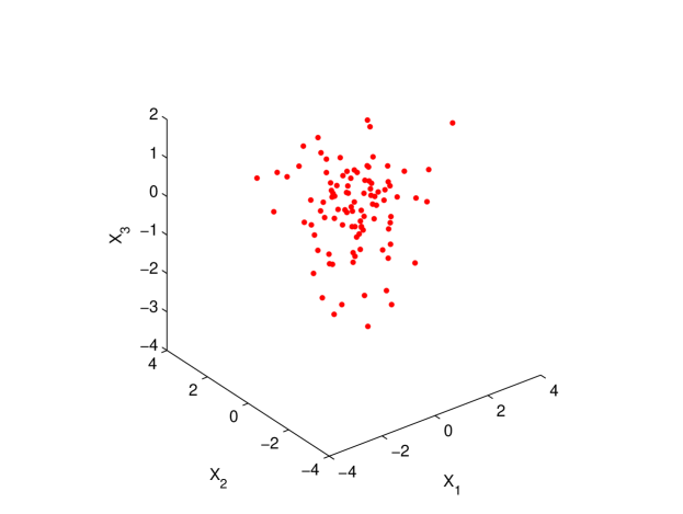
Figure 1: Shown is the scatter plot of the transformed IBM stock data from 2006 January 03 to 2006 May 25.

Table 1: The numbers of direction vectors and the computation times (in seconds) of the implementations of the proposed algorithm ($M_{n}$ and $T_{n}$) and that of Paindaveine and Šiman (2012b) ($M_{ps}$ and $T_{ps}$) for this transformed IBM stock data set.

$\tau$\		Number of direction vectors					Computation times
		$M_{n}$	$M_{ps}$	$M_{ps}/M_{n}$			$T_{n}$	$T_{ps}$	$T_{ps}/T_{n}$
0.01		86	328	3.81			0.033	0.934	28.22
0.05		499	2672	5.35			0.163	3.846	23.56
0.10		1195	6704	5.61			0.410	8.971	21.89
0.20		2732	13688	5.01			0.944	17.39	18.42
0.30		4663	29456	6.32			1.878	36.48	19.43
0.35		5106	33768	6.61			2.154	42.34	19.66

Furthermore, in order to gain more details about the proposed algorithm, we report the numbers of the $\tau$-th critical direction vectors obtained by the implementations of the proposed algorithm and that of Paindaveine and Šiman (2012b) for each depth region of this data set. It turns out that the new approach results in a much smaller number of direction vectors. For the given $\tau$, all of these numbers yielded by the proposed algorithm are smaller than the upper bound $100\times(100-1)$ as suggested by Corollary 1, in contrast to many cases of the method of Paindaveine and Šiman (2012b). As a result, the implementation of the proposed algorithm runs much faster than that of Paindaveine and Šiman (2012b); see Table 1 for details. Of course, there are some limitations in the comparison. That is, we compare just the implementations, and the direction vectors computed by the method of Paindaveine and Šiman (2012b) may contain some repetitions. But in any case, it seems reasonable to believe that the new method outperforms that of Paindaveine and Šiman (2012b) for this 3-dimensional data set.

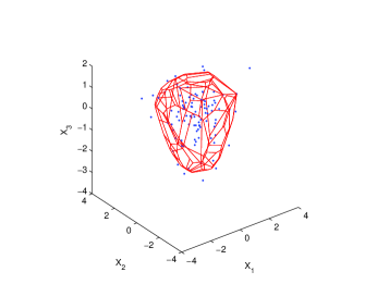
(a) $\tau=0.01$.

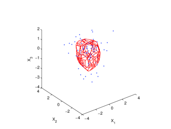
(b) $\tau=0.05$.

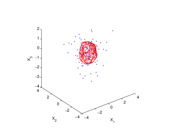
(c) $\tau=0.10$.

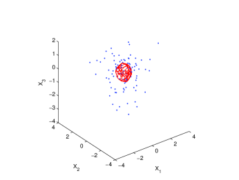
(d) $\tau=0.20$.

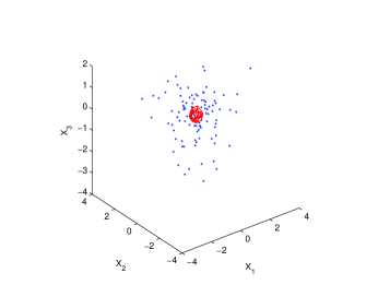
(e) $\tau=0.30$.

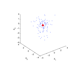
(f) $\tau=0.35$.

Figure 2: Shown are the $0.01,\,0.05,\,0.10,\,0.20,\,0.30,\,0.35$-th Tukey depth regions of the transformed IBM stock data from 2006 January 03 to 2006 May 25.

3.2 Simulated data

In the following, we further investigate the performance of the proposed algorithm with the simulated data, which are generated respectively from:

1. (D1). $(1-\varepsilon)N(\textbf{0}_{3},\mathbb{I}_{3})+\varepsilon N(\textbf{0}_{3},\sigma_{0}^{2}\mathbb{I}_{3})$.

2. (D2). $(1-\varepsilon)U([-0.5,\,0.5]^{3})+\varepsilon N(\textbf{0}_{3},\sigma_{0}^{2}\mathbb{I}_{3})$.

3. (D3). $(1-\varepsilon)N^{2}(\textbf{0}_{3},\Sigma_{3})+\varepsilon N(\textbf{0}_{3},\sigma_{0}^{2}\mathbb{I}_{3})$.

Here $\textbf{0}_{3}=(0,\,0,\,0)^{T}$, $\mathbb{I}_{3}$ is the identity matrix of order 3, $\sigma_{0}^{2}=9$, $U([-0.5,\,0.5]^{3})$ denotes the 3-dimensional uniform distribution over the region $[-0.5,\,0.5]\times[-0.5,\,0.5]\times[-0.5,\,0.5]$, and $N^{2}(\textbf{0}_{3},\Sigma_{3})$ is the distribution of $X=(Z_{1}^{2},\,Z_{2}^{2},\,Z_{3}^{2})$ such that $(Z_{1},\,Z_{2},\,Z_{3})$ is subject to $N(\textbf{0}_{3},\Sigma_{3})$, namely, the 3-dimensional normal distribution with mean zero and covariance-matrix

$$\Sigma_{3}=\left(\begin{array}[]{ccccc}1&&0.8&&0.8\\ 0.8&&4&&1.6\\ 0.8&&1.6&&4\end{array}\right).$$

For any combination of $n\in\{100,\,200,\,300,\,400,\,500,\,600\}$, $\tau\in\{$0.01, 0.05, 0.10, 0.20, 0.30$\}$ and $\varepsilon\in\{$0.00, 0.10, 0.20$\}$, we run the computation ten times for each scenario D.

The results are listed in Table 2-7. Similar to the case of real data above, the implementation of the proposed algorithm runs much faster than that of Paindaveine and Šiman (2012b), and results in a much smaller number ($\leq n(n-1)$) of direction vectors for each combination of $n$, $\tau$ and $\varepsilon$. The numbers in parentheses of these tables indicate how many times it is less than the benchmark of Paindaveine and Šiman (2012b).

Table 2: Average execution times (in seconds) of our Matlab code for Scenario (D1).

$\varepsilon$	$n$	$\tau$
		0.01	0.05	0.10	0.20	0.30
0.00	100	0.0395 (27.23)	0.1786 (15.56)	0.4329 (18.63)	1.1081 (17.91)	1.7990 (18.28)
	200	0.0888 (18.99)	0.6631 (16.47)	2.2206 (15.04)	9.0995 ( 8.94)	19.0790 ( 6.76)
	300	0.1944 (14.50)	2.0222 (17.45)	8.0355 (10.00)	39.0922 ( 5.21)	91.6904 ( 4.15)
	400	0.4097 (14.47)	4.8355 (10.26)	21.8888 ( 6.00)	125.9778 ( 2.74)	296.9387 ( 1.96)
	500	0.5888 (13.57)	9.7415 ( 8.58)	54.3214 ( 4.31)	321.8450 ( 2.45)	757.4869 ( 1.63)
0.10	100	0.0282 (26.49)	0.1727 (15.69)	0.4107 (15.60)	1.0235 (18.57)	1.8301 (17.20)
	200	0.0555 (19.57)	0.5575 (17.76)	1.8831 (13.44)	7.8327 ( 8.74)	17.1017 ( 6.33)
	300	0.0973 (22.51)	1.3544 (13.12)	6.1476 (11.46)	35.5195 ( 6.10)	90.3325 ( 3.84)
	400	0.1753 (12.02)	3.4345 (10.29)	17.7846 ( 6.84)	121.7643 ( 3.54)	328.2918 ( 2.22)
	500	0.3193 ( 9.69)	6.9518 ( 8.48)	44.1372 ( 4.17)	306.3422 ( 1.94)	750.4533 ( 1.44)
0.20	100	0.0142 (52.47)	0.1182 (17.40)	0.3828 (14.90)	0.9436 (13.96)	1.8105 (11.58)
	200	0.0551 (32.37)	0.4588 (15.93)	1.7513 (14.93)	8.0453 (10.35)	18.6599 ( 6.97)
	300	0.1110 (19.18)	1.1544 (16.82)	5.5883 (12.31)	37.7137 ( 5.75)	92.7185 ( 3.63)
	400	0.2024 (13.14)	2.7950 (15.16)	15.2962 ( 8.84)	118.5005 ( 3.37)	305.4019 ( 2.48)
	500	0.3905 (10.35)	5.0187 ( 8.96)	36.3917 ( 4.61)	290.2592 ( 2.26)	829.5661 ( 1.72)

Table 3: Average numbers of the critical directions vectors obtained by our Matlab code for Scenario (D1).

$\varepsilon$	$n$	$\tau$
		0.01	0.05	0.10	0.20	0.30
0.00	100	110 (3.27)	549 (3.32)	1333 (4.51)	3096 (5.03)	4492 (5.91)
	200	229 (3.07)	1713 (4.86)	4758 (4.70)	11772 (5.13)	18454 (5.34)
	300	409 (4.36)	3970 (6.78)	10880 (5.69)	25825 (6.06)	40188 (6.55)
	400	725 (5.73)	7031 (5.58)	18559 (5.50)	46478 (5.43)	70940 (5.49)
	500	841 (6.48)	10660 (5.98)	29139 (6.02)	73757 (6.79)	111743 (6.33)
0.10	100	86 (2.51)	509 (3.50)	1304 (3.80)	2968 (5.15)	4625 (5.55)
	200	144 (2.50)	1536 (4.97)	4342 (4.69)	11604 (4.77)	17782 (4.89)
	300	216 (6.26)	2932 (4.73)	9299 (6.03)	24891 (6.69)	40116 (6.44)
	400	327 (3.87)	5573 (5.03)	16975 (5.63)	46026 (6.04)	71964 (6.27)
	500	469 (3.89)	8221 (5.26)	25895 (4.95)	70744 (5.78)	110547 (5.95)
0.20	100	42 (5.14)	372 (3.20)	1209 (3.49)	2736 (3.74)	4605 (3.65)
	200	145 (6.01)	1245 (4.23)	4119 (5.02)	11706 (5.68)	18558 (5.56)
	300	248 (5.10)	2570 (5.78)	8632 (6.30)	25624 (6.48)	40566 (6.19)
	400	368 (3.91)	4687 (7.06)	15647 (6.65)	45278 (6.49)	72421 (7.00)
	500	580 (4.69)	6615 (5.27)	23736 (5.36)	69947 (5.89)	110834 (5.72)

Table 4: Average execution times (in seconds) of our Matlab code for Scenario (D2).

$\varepsilon$	$n$	$\tau$
		0.01	0.05	0.10	0.20	0.30
0.00	100	0.6356 ( 5.09)	0.2476 (15.30)	0.5190 (14.80)	1.1581 (15.63)	1.8583 (13.08)
	200	0.1370 (17.27)	1.0616 (12.28)	3.0077 (10.68)	9.3033 ( 9.17)	18.3017 ( 6.51)
	300	0.3542 (12.14)	2.9128 (12.09)	9.4009 ( 8.93)	44.0776 ( 4.43)	88.5952 ( 3.30)
	400	0.6518 (10.54)	7.7962 ( 8.69)	30.5603 ( 4.75)	143.1463 ( 2.48)	313.4953 ( 1.92)
	500	1.0839 ( 9.33)	14.3471 ( 7.40)	85.1707 ( 3.61)	412.3910 ( 1.76)	773.3136 ( 1.63)
0.10	100	0.0107 (43.12)	0.1426 (16.88)	0.4558 (14.35)	1.2381 (18.02)	2.0879 (21.91)
	200	0.0295 (43.57)	0.4748 (32.00)	2.7920 (30.53)	9.9825 (21.51)	24.5907 (13.63)
	300	0.1080 (26.98)	1.3357 (26.17)	9.3452 (19.46)	58.0981 ( 6.97)	121.2798 ( 4.63)
	400	0.1485 (22.31)	3.3645 (12.43)	28.2102 ( 6.08)	189.8710 ( 2.40)	339.9063 ( 2.09)
	500	0.2476 (10.17)	5.6117 ( 6.39)	54.9067 ( 3.65)	363.9800 ( 1.71)	904.9331 ( 1.66)
0.20	100	0.0097 (49.30)	0.1454 (46.94)	0.4791 (35.52)	1.2875 (27.31)	2.2747 (20.94)
	200	0.0783 (70.00)	0.3573 (35.06)	1.5052 (13.38)	11.8260 (12.42)	30.0845 ( 6.93)
	300	0.1365 (21.00)	0.7410 (20.36)	7.3669 (13.85)	71.6315 ( 4.70)	99.6734 ( 4.93)
	400	0.2389 ( 9.32)	1.5917 ( 9.59)	9.2006 ( 8.96)	136.7832 ( 2.62)	318.7450 ( 1.90)
	500	0.3642 (12.77)	2.3915 (12.11)	23.5790 ( 7.14)	324.9054 ( 2.98)	947.2455 ( 2.37)

Table 5: Average numbers of the critical directions vectors obtained by our Matlab code for Scenario (D2).

$\varepsilon$	$n$	$\tau$
		0.01	0.05	0.10	0.20	0.30
0.00	100	158 (1.82)	706 (3.65)	1530 ( 3.87)	3177 ( 4.38)	4433 ( 4.40)
	200	348 (3.77)	2474 (4.04)	5815 ( 4.33)	12642 ( 5.08)	17635 ( 5.19)
	300	761 (4.18)	5311 (5.33)	12155 ( 5.56)	27603 ( 5.55)	39579 ( 5.45)
	400	1039 (4.18)	9080 (5.31)	21581 ( 5.10)	48867 ( 5.12)	71233 ( 5.59)
	500	1555 (4.75)	13913 (5.81)	34190 ( 5.84)	75604 ( 6.13)	110543 ( 6.31)
0.10	100	28 (7.14)	402 (3.16)	1326 ( 3.23)	3206 ( 4.98)	4666 ( 6.82)
	200	72 (4.67)	1156 (8.62)	5017 (11.74)	12301 (11.52)	17999 (10.57)
	300	156 (6.87)	2269 (8.36)	10245 (10.04)	27082 ( 8.94)	41002 ( 8.43)
	400	227 (6.10)	4709 (5.34)	18677 ( 5.45)	48235 ( 5.44)	72222 ( 5.91)
	500	346 (3.82)	6894 (3.61)	28449 ( 4.84)	76065 ( 5.09)	112214 ( 5.51)
0.20	100	24 (6.67)	359 (9.67)	1234 ( 8.08)	3108 ( 6.93)	4621 ( 5.99)
	200	134 (3.17)	718 (7.73)	2977 ( 3.69)	12182 ( 6.71)	18399 ( 6.21)
	300	198 (5.41)	1270 (6.03)	8558 ( 6.60)	26497 ( 7.80)	41445 ( 8.13)
	400	410 (2.56)	2802 (3.69)	10842 ( 5.37)	46060 ( 4.75)	74152 ( 5.38)
	500	562 (5.40)	3672 (6.01)	19369 ( 6.43)	74498 ( 7.74)	116429 ( 7.33)

Table 6: Average execution times (in seconds) of our Matlab code for Scenario (D3).

$\varepsilon$	$n$	$\tau$
		0.01	0.05	0.10	0.20	0.30
0.00	100	0.0534 (37.66)	0.2405 ( 5.41)	0.5330 (30.86)	1.1696 (35.98)	1.8622 (27.92)
	200	0.1588 (27.16)	0.9540 (32.09)	3.2558 (23.56)	9.1112 (14.81)	17.2464 (10.89)
	300	0.2830 (23.84)	2.5542 (23.08)	8.7608 (14.34)	46.8278 ( 7.25)	98.1411 ( 5.26)
	400	0.6128 (18.36)	6.7065 (15.19)	30.4956 ( 9.43)	136.3922 ( 4.55)	275.2976 ( 3.61)
	500	1.1261 (15.00)	13.9530 (11.39)	72.2767 ( 6.24)	361.9681 ( 3.63)	721.6153 ( 2.97)
0.10	100	0.0210 (48.32)	0.1645 (37.49)	0.4441 (36.57)	1.3561 (31.72)	2.1059 (24.11)
	200	0.0593 (33.34)	0.7486 (31.92)	2.8938 (29.51)	9.7552 (17.97)	18.2607 (12.44)
	300	0.1063 (19.33)	1.4610 (18.87)	7.8851 (16.40)	42.3759 ( 7.43)	91.0750 ( 5.02)
	400	0.2257 (16.76)	2.5603 (14.12)	21.8409 (15.81)	119.8576 ( 6.80)	304.2660 ( 4.12)
	500	0.3739 (13.30)	4.8199 (12.03)	43.9444 (10.74)	312.6973 ( 5.15)	777.7728 ( 3.45)
0.20	100	0.0324 (49.54)	0.1342 (33.42)	0.3001 (33.00)	1.0985 (43.20)	1.9382 (33.24)
	200	0.0787 (27.05)	0.5317 (22.81)	1.9892 (32.72)	9.0659 (18.86)	18.6073 (13.36)
	300	0.1234 (23.46)	1.1977 (19.86)	5.3343 (15.52)	39.0659 ( 9.93)	95.4297 ( 6.21)
	400	0.2734 (24.97)	2.4064 (15.15)	10.4868 ( 7.88)	115.3662 ( 5.63)	380.4795 ( 3.54)
	500	0.5063 (12.92)	5.9210 (10.24)	31.7895 ( 8.85)	335.6343 ( 4.56)	790.5407 ( 3.97)

Table 7: Average numbers of the critical directions vectors obtained by our Matlab code for Scenario (D3).

$\varepsilon$	$n$	$\tau$
		0.01	0.05	0.10	0.20	0.30
0.00	100	213 ( 4.06)	785 (5.23)	1666 ( 7.34)	3445 ( 8.26)	4894 ( 7.77)
	200	603 ( 3.79)	3222 (6.57)	7012 ( 7.55)	13625 ( 6.99)	18968 ( 6.85)
	300	929 ( 4.63)	5703 (7.00)	12974 ( 7.06)	29113 ( 7.60)	42981 ( 7.68)
	400	1649 ( 4.55)	11528 (6.40)	26891 ( 7.25)	53417 ( 7.28)	73666 ( 7.13)
	500	2286 ( 4.89)	16515 (6.43)	38561 ( 7.20)	81172 ( 7.92)	114403 ( 7.85)
0.10	100	59 ( 4.61)	547 (6.93)	1406 ( 8.03)	3401 ( 8.32)	4793 ( 6.98)
	200	132 ( 4.67)	2030 (7.36)	5995 ( 9.26)	13194 ( 9.13)	19061 ( 7.98)
	300	225 ( 4.98)	3340 (5.83)	12077 ( 7.71)	29041 ( 7.43)	41614 ( 7.18)
	400	393 ( 5.72)	4145 (5.93)	19838 (11.40)	48840 ( 9.62)	75828 ( 8.34)
	500	549 ( 5.79)	6351 (6.68)	29920 (10.23)	79100 ( 9.51)	119544 ( 8.70)
0.20	100	90 ( 8.62)	407 (7.25)	890 ( 8.09)	3208 (11.07)	4848 (10.16)
	200	191 ( 6.03)	1361 (6.46)	4915 ( 9.79)	13290 ( 9.31)	19472 ( 9.03)
	300	259 ( 7.01)	2487 (7.23)	8245 ( 7.46)	27363 ( 9.63)	43011 ( 8.69)
	400	459 (10.16)	3970 (6.91)	12053 ( 5.07)	46801 ( 8.39)	75364 ( 8.60)
	500	686 ( 6.02)	6970 (6.24)	22555 ( 8.22)	75553 ( 9.21)	117714 ( 8.17)

4 Concluding remarks

In this paper, we have constructed a fast algorithm for computing a 3-dimensional $\tau$-Tukey depth region. Rather than searching the critical direction vectors cone-by-cone, the proposed algorithm finds all possible direction vectors subscript-tuple-by-subscript-tuple. Consequently, checking directly the values of $\mathcal{A}_{i_{0},j_{0}}$ and $\mathcal{T}_{i_{0},j_{0}}$ is sufficient to determine if a newly obtained subscript tuple $[i_{0},\,j_{0}]$ has been investigated. This new searching tactics helps to avoid some unnecessary repeated checks and in turn save considerable computational times. The data examples indicate that our results provide a significant speed-up over existing algorithms.

In the literature, there are many other depth notions, such as projection depth and zonoid depth, closely related to the methodology of projection pursuit. It turns out that most of them can be exactly computed from the view of cutting a convex polytope with hyperplanes; see Mosler et al. (2009) and Liu and Zuo (2014) respectively for details. Then a natural question concerns faster algorithms for these depth notions. This may be of great practice interest, because some of these depth notions could not be computed efficiently in dimensions of $p\geq 3$. Work is underway.

Appendix

$\square$ (A.1) Find an initial subscript tuple $[i_{0},\,j_{0}]$. In Step 2.2, we compute $[i_{0},\,j_{0}]$ by using the following procedure.

1. 2.2.1. Generate a random unit vector $u_{0}$, and store the permutation $(i_{1},\,i_{2},\,\cdots,\,i_{n})$ such that $u_{0}^{T}X_{i_{1}}<u_{0}^{T}X_{i_{2}}<\cdots<u_{0}^{T}X_{i_{n}}$.

2. 2.2.2. Compute the distances $\theta_{i}$’s between the point $u_{0}$ and $n-1$ hyperplanes $\mathcal{P}_{i}=\{s\in\mathcal{R}^{p}:(X_{i}-X_{i_{k_{\tau}}})^{T}s=0\}$, where $i\in\mathcal{N}$ and $i\neq i_{k_{\tau}}$.

3. 2.2.3. Find the minimum among $\theta_{i}$’s and obtain the corresponding subscript tuple $[i^{*},\,i_{k_{\tau}}]$. Assign the maximum of $\{i^{*},\,i_{k_{\tau}}\}$ to $i_{0}$ and the other one to $j_{0}$, respectively.

This procedure corresponds to the code snippets between lines 48-58 of FHC3D.m; see Appendix (A.5). The rational behind is as follows. By $u_{0}^{T}X_{i_{1}}<u_{0}^{T}X_{i_{2}}<\cdots<u_{0}^{T}X_{i_{n}}$, it is easy to show that $u_{0}\in\mathcal{C}=\{t:\mathbb{A}_{0}^{T}t\leq 0\}$, where

$$\mathbb{A}_{0}=(X_{i_{1}}-X_{i_{k_{\tau}}},\,X_{i_{2}}-X_{i_{k_{\tau}}},\,\cdots,\,X_{i_{k_{\tau}-1}}-X_{i_{k_{\tau}}},\,X_{i_{k_{\tau}}}-X_{i_{k_{\tau}+1}},\,\cdots,\,X_{i_{k_{\tau}}}-X_{i_{n}}).$$

Clearly, $\mathcal{C}$ forms a polytope, on each vertex of which must lie an $\tau$-critical direction vectors. The closest hyperplane to $u_{0}$ must pass through a non-redundant facet of $\mathcal{C}$, and hence its corresponding subscript tuple $[i^{*},\,i_{k_{\tau}}]$ is what we want. $\square$

$\square$ (A.2) Find all the possible subscripts $k_{0}$. In Step 2.3, we utilize the following procedure to to find all the possible subscripts $k_{0}$.

1. 2.3.k1. Project the data points $X_{k}$ $(k\in\mathcal{N}/\{i_{0},\,j_{0}\})$ onto the plane $\mathcal{P}_{0}$, which is perpendicular to $\alpha_{0}=\frac{X_{i_{0}}-X_{j_{0}}}{\|X_{i_{0}}-X_{j_{0}}\|}$ and pass through $X_{j_{0}}$. Without loss of generality, denote the projection of $X_{k}$ as $X_{k}^{*}$.

2. 2.3.k2. Compute the polar coordinate angles $\theta_{k}$ $(\theta_{k}\in[-\pi,\,\pi))$ of $(\beta_{k1},\,\beta_{k2})$ if $\alpha_{03}\neq 0$ (otherwise, use $(\beta_{k2},\,\beta_{k3})$ instead of $(\beta_{k1},\,\beta_{k2})$), where $\beta_{k}:=(\beta_{k1},\,\beta_{k2},\,\beta_{k3})^{T}=\frac{X_{k}^{*}-X_{j_{0}}}{\|X_{k}^{*}-X_{j_{0}}\|}$ $(k\in\mathcal{N}/\{i_{0},\,j_{0}\})$ and $\alpha_{03}$ denotes the third component of $\alpha_{0}$.

3. 2.3.k3. For each $k\in\mathcal{N}/\{i_{0},\,j_{0}\}$, count the number $N_{1}$ of these polar coordinate angles that lie in $(\theta_{k},\,\theta_{k}+\pi)$ and the number $N_{2}$ of those that lie in $(-\pi,\,\theta_{k})\bigcup(\theta_{k}+\pi,\,\pi)$. If either $N_{1}$ or $N_{2}$ is equal to $\lfloor n\tau\rfloor$, then $k$ is a satisfactory subscript.

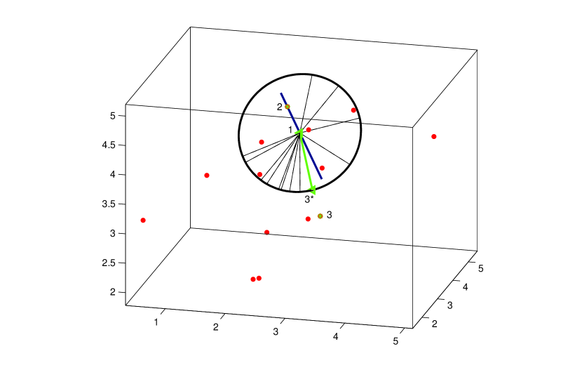
Figure 3: Shown is an illustration of how to find the possible subscripts $k_{0}$. The points denote the observations. Every point (not in the line passing through points 1 and 2) corresponds to a unit vector stemming from point 1 in $\mathcal{P}_{0}$.

This part can be easily implemented by using the Gram-Schmidt orthonormalization. The corresponding Matlab code lie between lines 67-87 of FHC3D.m; see Appendix (A.5). As illustration of this procedure is provided in Figure 3. In this figure, points 1 and 2 serve as the points $X_{j_{0}}$ and $X_{i_{0}}$, respectively. Then every point $X_{k}$ $(k\in\mathcal{N}/\{i_{0},\,j_{0}\})$ corresponds to the polar coordinate angle of one unit vector in $\mathcal{P}_{0}$ passing through point 1. For example, $\alpha_{0}$ lies in the line pass through points 1 and 2, and point 3 corresponds to the angle of the vector connecting points 1 and $3^{*}$. It is easy to see that the plane passing through points 1, 2 and 3 divides the whole space $\mathcal{R}^{3}$ into two halfspace spaces with 4 data points on one side, and 12 data points on the other side. A similar procedure of such kind is the planar algorithm developed by Rousseeuw and Struyf (1998) (pp. 201-202). $\square$

$\square$ (A.3) Proof of Theorem 1. For a given $\tau$, let $k_{\tau}=\lfloor n\tau\rfloor+1$. Note that for any $u_{0}\in\mathcal{S}^{p-1}$, there must exist a permutation $(j_{1},\,j_{2},\,\cdots,\,j_{n})$ of $(1,\,2,\,\cdots,\,n)$ such that $u^{T}X_{j_{1}}<u^{T}X_{j_{2}}<\cdots<u^{T}X_{j_{n}}$. Using this, one can, similar to Liu et al. (2013), obtain that

$$\mathcal{S}^{p-1}=\bigcup_{l=1}^{M_{s}}\mathcal{S}_{l},\quad\text{with}\quad\mathcal{S}_{l}=\{u\in\mathcal{S}^{p-1}:A_{l}^{T}u\leq 0\},$$

where $M_{s}$ denotes the number of $\mathcal{S}_{l}$ and

$$\mathbb{A}_{l}=(X_{j_{l,1}}-X_{j_{l,k_{\tau}}},\,X_{j_{l,2}}-X_{j_{l,k_{\tau}}},\,\cdots,\,X_{j_{l,k_{\tau}-1}}-X_{j_{l,k_{\tau}}},\,X_{j_{l,k_{\tau}}}-X_{j_{l,k_{\tau}+1}},\,\cdots,\,X_{j_{l,k_{\tau}}}-X_{j_{l,n}}).$$

Denote $\mathcal{C}_{l}=\{t\in\mathcal{R}^{p}:A_{l}^{T}t\leq 0\}$ ($1\leq l\leq M_{s}$). Clearly, $\mathcal{S}_{l}\subset\mathcal{C}_{l}$ and $\mathcal{C}_{l}$’s are convex cones. Without loss of generality, assume $\mathcal{C}_{l}$ has $m_{l}$ vertices, and let $\widetilde{u}_{l,1},\,\widetilde{u}_{l,2},\,\cdots,\,\widetilde{u}_{l,m_{l}}\ (\in\mathcal{S}_{l}\cap\mathcal{C}_{l})$ to be the unit direction vectors corresponding to these vertices. By the convexity of $\mathcal{C}_{l}$ and the fact that $\widetilde{u}_{l,1}^{T}x\geq\widetilde{u}_{l,1}^{T}X_{j_{l,k_{\tau}}}$, $\cdots$, $\widetilde{u}_{l,m_{l}}^{T}x\geq\widetilde{u}_{l,m_{l}}^{T}X_{j_{l,k_{\tau}}}$ together lead to $(\sum_{i=1}^{m_{l}}\lambda_{i}\widetilde{u}_{l,i})^{T}x\geq(\sum_{i=1}^{m_{l}}\lambda_{i}\widetilde{u}_{l,i})^{T}X_{j_{l,k_{\tau}}}$, it is easy to show that

$$\bigcap_{u\in\mathcal{C}_{l}}\left\{x\in\mathcal{R}^{p}:u^{T}x\geq u^{T}X_{j_{l,k_{\tau}}}\right\}=\bigcap_{u\in\mathcal{S}_{l}}\left\{x\in\mathcal{R}^{p}:u^{T}x\geq u^{T}X_{j_{l,k_{\tau}}}\right\}=\bigcap_{i=1}^{m_{l}}\left\{x\in\mathcal{R}^{p}:\widetilde{u}_{l,i}^{T}x\geq\widetilde{u}_{l,i}^{T}X_{j_{l,k_{\tau}}}\right\},$$

where $\lambda_{i}\geq 0$, $i=1,\,2,\,\cdots,\,m_{l}$. This implies that the exact computation of $\mathcal{D}_{\tau}$ depends only on a finite number of unit direction vectors corresponding to the vertices of $\mathcal{C}_{l}$, $l=1,\,\cdots,\,M_{s}$.

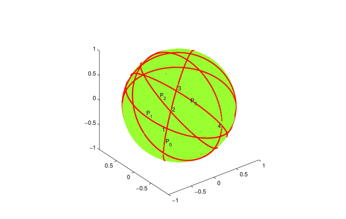
Figure 4: Shown is an illustration of the linked points on the unit sphere $\mathcal{S}^{2}$. Here points 2 and 4 are linked through the arcs between points 2, 3 and 4.

When $p=3$, a vertex of $\mathcal{C}_{l}$ is determined by two non-redundant facets, which are determined by three observations. Every two points, corresponding to two critical direction vectors, on the sphere $\mathcal{S}^{2}$ are linked with each other through some arcs if the observations are in general position; see points 1 and 4 in Figure 4 for an illustration. A subscript tuple, corresponding to two observations, determines a non-redundant facet, which may contain several critical direction vectors. Enumerating all such subscript tuples, namely, iterating Steps 2.3-2.6, can find the critical direction vectors, by using which it is sufficient to obtain an exact Tukey depth region. $\square$

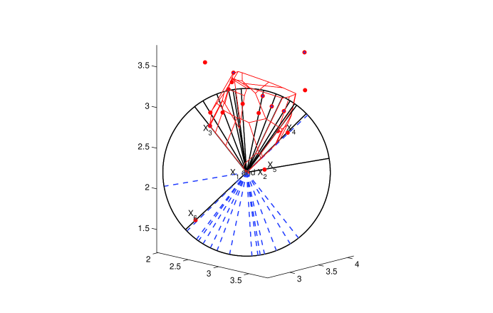
Figure 5: 5 is the $0.01$-th Tukey depth region of a data set with sample size $n=20$. For this case, $k_{\tau}=1$, and there are four $\tau$-critical hyperplanes passing through $X_{1}$, $X_{2}$ (and $X_{3}$, $X_{4}$, $X_{5}$, $X_{6}$, respectively). Among them, only two hyperplanes, through $\{X_{1}$, $X_{2}$, $X_{3}\}$ and $\{X_{1}$, $X_{2}$, $X_{4}\}$ respectively, yield two $non$-redundant facets by the convexity of $\mathcal{D}_{\tau}$; see 5.

$\square$ (A.4) Proof of Corollary 1. Without loss of generality, we call a hyperplane $\tau$-critical hyperplane if it passes though three observations and divides the whole space into two parts with $\lfloor n\tau\rfloor$ on one side and the rest on the other side. By the convexity of the Tukey depth region, a $\tau$-critical hyperplane yields at most one facet of $\mathcal{D}_{\tau}$. When $p=3$ and the observations are in general position, although every two observations $X_{i_{0}}$ and $X_{j_{0}}$, corresponding to $[i_{0},\,j_{0}]$, may be contained in more than two $\tau$-critical hyperplanes, at most two of these $\tau$-critical hyperplanes are possible to yield $non$-redundant facets of $\mathcal{D}_{\tau}$; see Figure 5 for an illustration. The proves that the number of $non$-redundant facets of $\mathcal{D}_{\tau}$ is at most $2\times{n\choose 2}=n(n-1)$. $\square$

$\square$ (A.5) Code snippet. The main function FHC3D.m corresponding to the proposed algorithm. It is construed mainly for computing the $\tau$-critical direction vectors of a given Tukey depth region.

⬇

1% FHC3D.m

2%

3% Description:

4%

5% Fast computing the critical direction vectors of the tau-th

6% Tukey depth region for a 3-dimensional X.

7%

8% Input arguments:

9% X - data matrix, n-by-3 (matrix), n denotes the

10% sample size

11% tau0 - depth value of the computed contour

12% (0 <= tau0 < tau0Star (the maximum depth

13% value))

14%

15% Output arguments:

16% vecu - struct(’u’, [], ’QuanV’, [], ’NumU’, [])

17

18

19function vecu = FHC3D(X, tau0)

20

21 % Check the input arguments

22 [n, p] = size(X);

23 if p ~= 3, error(’X must be an n-by-3 matrix!’); end

24

25 % Initialize vecu

26 vecu.u = []; vecu.QuanV = []; vecu.NumU = 0;

27

28 % Initialize the archives NewIndx and OldIndx.

29 % ’NewIndx(i, j) = true’ means that Xi - Xj needs to be considered;

30 % ’OldIndx(i, j) = true’ means that Xi - Xj has been considered.

31 NewIndx = false(n, n); OldIndx = false(n, n);

32

33 % The sub-index tauk corresponding to tau0

34 taukSUB1 = floor(n * tau0); tauk = taukSUB1 + 1;

35

36 % Initialize some intermediate variables

37 nSUB1 = n - 1; nSUB2 = n - 2;

38 nDIV4 = floor(n / 4);

39 ONESn1X1 = ones(nSUB1, 1); ONESn2X1 = ones(nSUB2, 1);

40 ONESpX1 = ones(p, 1); piMULT2 = 2 * pi;

41 nSubtauk1 = nSUB2 - taukSUB1; nSubtauk2 = nSubtauk1 - 1;

42 VecN1 = 1:nSUB2;

43 LowIndx1 = VecN1 + taukSUB1; UpIndx1 = VecN1 + tauk;

44 LowIndx2 = VecN1 + nSubtauk2; UpIndx2 = VecN1 + nSubtauk1;

45 LowIndx3 = LowIndx2 - nDIV4; UpIndx3 = UpIndx1 + nDIV4;

46

47 % Obtain an intial index-couple [rowi, colj]

48 IndxSet = [1:(tauk - 1), (tauk + 1):n];

49 IPVec = ONESpX1 / norm(ONESpX1);

50 [sortXu, perm0] = sort(X * IPVec);

51 QuanX = X(perm0, :);

52 % Obtain the normal vectors of {u: u^T * (X(i, :) - X(j, :))}

53 NVec = (QuanX(IndxSet, :) - ONESn1X1 * QuanX(tauk, :));

54 NVec(tauk:nSUB1, :) = -NVec(tauk:nSUB1, :);

55 NVec = NVec ./ (sqrt(sum(NVec.^2, 2)) * ONESpX1’);

56 [tmpv, tmpk] = min(abs(NVec * IPVec));

57 rowi = max(perm0(IndxSet(tmpk(1))), perm0(tauk));

58 colj = min(perm0(IndxSet(tmpk(1))), perm0(tauk));

59

60 % Update NewIndx and OldIndx

61 NewIndx(rowi, colj) = true;

62 OldIndx(rowi, colj) = true;

63

64 % Compute all the optimal direction vectors

65 while any(any(NewIndx)) % If NewIndx(i, j) = true

66 [rowi, colj] = find(NewIndx, 1);

67 IndxSet = [1:(colj - 1), (colj + 1):(rowi - 1), (rowi + 1):n];

68 % The vector Xi - Xj

69 alpha0 = X(rowi, :) - X(colj, :);

70 alpha0 = alpha0 / norm(alpha0);

71 % The vectors Xk - Xj (k in {1, 2, ..., n} - {i, j})

72 beta0 = X(IndxSet, :) - ONESn2X1 * X(colj, :);

73 gamma0 = beta0 - (beta0 * alpha0’) * alpha0;

74 tmpvec = gamma0(:, 1);

75 if abs(alpha0(3)) < 1e-12, tmpvec = gamma0(:, 3); end

76 isvec0 = (tmpvec < 0);

77 theta0 = atan(gamma0(:, 2) ./ tmpvec) + ...

78 (isvec0 & (gamma0(:, 2) > 0)) * pi - ...

79 (isvec0 & (gamma0(:, 2) < 0)) * pi;

80 % Sort theta0

81 [theta0, perm0] = sort(theta0);

82 theta1 = [theta0; theta0(1:nSubtauk1) + piMULT2];

83 perm1 = [perm0; perm0(1:nSubtauk1)];

84

85 UpBnd = theta0 + pi;

86 isvec1 = (theta1(LowIndx1) < UpBnd) & (UpBnd < theta1(UpIndx1));

87 isvec2 = (theta1(LowIndx2) < UpBnd) & (UpBnd < theta1(UpIndx2));

88

89 % Update vecu

90 newl1 = perm1(UpIndx3(isvec1));

91 newl2 = perm1(VecN1(isvec1));

92 for ll = 1:length(newl1)

93 tmpu0 = gamma0(newl2(ll), :) / norm(gamma0(newl2(ll), :));

94 tmpu1 = gamma0(newl1(ll), :) - (gamma0(newl1(ll), :) * tmpu0’) * tmpu0;

95 tmpu1 = tmpu1’ / norm(tmpu1);

96 tmpv = X(rowi, :) * tmpu1;

97 vecu.u = [vecu.u, tmpu1];

98 vecu.QuanV = [vecu.QuanV; tmpv];

99 vecu.NumU = vecu.NumU + 1;

100 end

101 newl1 = perm1(LowIndx3(isvec2));

102 newl2 = perm1(VecN1(isvec2));

103 for ll = 1:length(newl1)

104 tmpu0 = gamma0(newl2(ll), :) / norm(gamma0(newl2(ll), :));

105 tmpu1 = gamma0(newl1(ll), :) - (gamma0(newl1(ll), :) * tmpu0’) * tmpu0;

106 tmpu1 = tmpu1’ / norm(tmpu1);

107 tmpv = X(rowi, :) * tmpu1;

108 vecu.u = [vecu.u, tmpu1];

109 vecu.QuanV = [vecu.QuanV; tmpv];

110 vecu.NumU = vecu.NumU + 1;

111 end

112

113 % Update NewIndx and OldIndx

114 newl2 = perm0(isvec1 | isvec2);

115 for ll = 1:length(newl2)

116 tmpv1 = sort([rowi, IndxSet(newl2(ll))], ’descend’);

117 tmpv2 = sort([colj, IndxSet(newl2(ll))], ’descend’);

118 if ~OldIndx(tmpv1(1), tmpv1(2)), NewIndx(tmpv1(1), tmpv1(2)) = true; end

119 if ~OldIndx(tmpv2(1), tmpv2(2)), NewIndx(tmpv2(1), tmpv2(2)) = true; end

120 OldIndx(tmpv1(1), tmpv1(2)) = true;

121 OldIndx(tmpv2(1), tmpv2(2)) = true;

122 end

123

124 % Eliminate NewIndx(rowi, colj) from the next consideration

125 NewIndx(rowi, colj) = false;

126 end

127 % Eliminate the repetitions from vecu

128 [tmpv, indx] = unique(num2str(vecu.u’, 12), ’rows’);

129 vecu.u = vecu.u(:, indx);

130 vecu.QuanV = vecu.QuanV(indx);

131 vecu.NumU = length(indx);

132

133% End of program

$\square$

References

- Agostinelli and Romanazzi (2011) Agostinelli, C., Romanazzi, M. 2011. Local depth. Journal of Statistical Planning and Inference, 141(2), 817-830.
- Barber et al. (1996) Barber, C.B., Dobkin, D.P., Huhdanpaa, H., 1996. The quickhull algorithm for convex hulls. ACM Transactions Math. Software 22, 469-483.
- Hallin et al. (2010) Hallin, M., Paindaveine, D., Šiman, M., 2010. Multivariate quantiles and multiple-output regression quantiles: From optimization to halfspace depth. Ann. Statist. 38, 635-669.
- Li et al. (2012) Li, J., Cuesta-Albertos, J.A., Liu, R.Y., 2012. DD-classifier: nonparametric classification procedure based on DD-plot. J. Amer. Statist. Assoc. 107(498), 737-753.
- Liu (1990) Liu, R.Y., 1990. On a notion of data depth based on random simplices. Ann. Statist. 18, 191-219.
- Liu (1992) Liu, R.Y., 1992. Data depth and multivariate rank tests. In L1-Statistical Analysis and Related Methods (Y. Dodge, ed.), 279-294. North-Holland, Amsterdam.
- Liu et al. (2013) Liu, X.H., Zuo, Y.J., Wang, Z.Z., 2013. Exactly computing bivariate projection depth median and contours. Comput. Statist. Data Anal. 60, 1-11.
- Liu and Zuo (2014) Liu, X.H., Zuo, Y.J., 2014. Computing projection depth and its associated estimators. Statistics and Computing, 24(1), 51-63.
- Kong and Mizera (2008) Kong, L., Mizera, I., 2008. Quantile tomography: Using quantiles with multivariate data. Statist. Sinica, 22, 1589-1610.
- Koshevoy and Mosler (1997) Koshevoy, H., Mosler, K., 1997. Zonoid trimming for multivariate distributions. Ann. Statist. 25, 1998-2017.
- Mosler et al. (2009) Mosler, K., Lange, T., Bazovkin, P., 2009. Computing zonoid trimmed regions of dimension . Comput. Statist. Data Anal. 53, 2500-2510.
- Paindaveine and Šiman (2011) Paindaveine, D., Šiman, M., 2011. On directional multiple-output quantile regression. J. Multivariate Anal. 102, 193-392.
- Paindaveine and Šiman (2012a) Paindaveine, D., Šiman, M., 2012a. Computing multiple-output regression quantile regions. Comput. Statist. Data Anal. 56, 840-853.
- Paindaveine and Šiman (2012b) Paindaveine, D., Šiman, M., 2012b. Computing multiple-output regression quantile regions from projection quantiles. Comput. Statist. 27, 29-49.
- Paindaveine and Van bever (2012) Paindaveine, D., Van Bever, G. 2012, Nonparametrically consistent depth-based classifiers. conditionally accepted in Bernoulli.
- Paindaveine and Van bever (2013) Paindaveine, D., Van bever, G., 2013. From Depth to Local Depth: A Focus on Centrality. J. Amer. Statist. Assoc. 108(503), 1105-1119.
- Rousseeuw and Struyf (1998) Rousseeuw, P.J., Struyf, A., 1998. Computing location depth and regression depth in higher dimensions. Statist. Comput. 8, 193-203.
- Ruts and Rousseeuw (1996) Ruts, I., Rousseeuw, P.J., 1996. Computing depth contours of bivariate point clouds. Comput. Statist. Data Anal. 23, 153-168.
- Tsay (2010) Tsay, R.S., 2010. Analysis of Financial Time Series, Third Edition. John Wiley & Sons.
- Tukey (1975) Tukey, J.W., 1975. Mathematics and the picturing of data. In Proceedings of the International Congress of Mathematicians, 523-531. Cana. Math. Congress, Montreal.
- Yeh and Singh (1997) Yeh, A., Singh, K., 1997. Balanced confidence regions based on Tukey’s depth and the bootstrap. J. Roy. Statist. Soc. Ser. B 59, 639-652.
- Zuo (2003) Zuo, Y.J., 2003. Projection based depth functions and associated medians. Ann. Statist. 31, 1460-1490.
- Zuo and Serfling (2000) Zuo, Y.J., Serfling, R., 2000. General notions of statistical depth function. Ann. Statist. 28, 461-482.