The ballistic transport instability in Saturn’s rings II: nonlinear wave dynamics

Abstract

The ejecta discharged by impacting meteorites can redistribute a planetary ring’s mass and angular momentum. This ‘ballistic transport’ of ring properties instigates a linear instability that could generate the 100–1000-km undulations observed in Saturn’s inner B-ring and in its C-ring. We present semi-analytic results demonstrating how the instability sustains steadily travelling nonlinear wavetrains. At low optical depths, the instability produces approximately sinusoidal waves of low amplitude, which we identify with those observed between radii 77,000 and 86,000 km in the C-ring. On the other hand, optical depths of 1 or more exhibit hysteresis, whereby the ring falls into multiple stable states: the homogeneous background equilibrium or large-amplitude wave states. Possibly the ‘flat zones’ and ‘wave zones’ between radii 93,000 and 98,000 km in the B-ring correspond to the stable homogeneous and wave states, respectively. In addition, we test the linear stability of the wavetrains and show that only a small subset are stable. In particular, stable solutions all possess wavelengths greater than the lengthscale of fastest linear growth. We supplement our calculations with a weakly nonlinear analysis that suggests the C-ring reproduces some of the dynamics of the complex Ginzburg–Landau equation. In the third paper in the series, these results will be tested and extended with numerical simulations.

1 Introduction

The component particles of planetary rings suffer a continual bombardment of hypervelocity meteoroids, the impacts of which liberate a significant amount of material. Typically, impact ejecta reaccrete on to the ring but at a different radius from where they originated; they hence redistribute its mass and angular momentum. This ‘ballistic transport’ of ring properties occurs on a characteristic lengthscale $l_{\text{th}}\sim 10-10^{3}$ km (the ‘throw length’) and a timescale $t_{e}\sim 10^{5}-10^{7}$ yr (the ‘erosion time’) (Durisen 1984, Ip 1984, Lissauer 1984). Other than influencing the large-scale evolution of Saturn’s rings, ballistic transport instigates a linear instability that can spontaneously create structure on these scales (Durisen 1995). It has been argued that the 100-km waves in the inner B-ring and the 1000-km undulations in the C-ring are a result of the instability’s nonlinear saturation (Durisen et al. 1992, hereafter D92, Durisen 1995, Charnoz et al. 2009, Colwell et al. 2009).

This is the second paper in a series devoted to the dynamics of the ballistic transport instability (BTI) and its generation of axisymmetric structure. The first paper, Latter et al. (2012) (hereafter Paper 1), outlined a convenient theoretical framework within which to attack the problem and rederived the BTI’s linear theory. Here we aim to go further by tracking the BTI’s nonlinear saturation. Ultimately, one is obliged to numerically simulate its evolution, and we present such calculations in the third paper of the series (Latter et al. 2013, submitted, hereafter Paper 3). In this work, however, we take a dynamical systems approach and establish a set of ‘a priori’ results that can both guide and explain the simulations.

First we demonstrate that ballistic transport supports families of steadily travelling nonlinear wavetrains. These solutions may be computed directly from the system’s governing evolution equation. At low optical depths $\tau$, the wavetrains assume small amplitudes and possess approximately sinusoidal profiles.We identify them with the long 1000-km undulations in the C-ring between radii 77,000 and 86,000 km (see Fig. 13.17 in Colwell et al. 2009), but conclude that the 100-km plateaus at slightly larger radii are not generated by the BTI, at least not working in isolation. Meanwhile, when $\tau\gtrsim 1$ the system exhibits hysteresis: the homogeneous state is linearly stable, but there exist additional wave solutions of large amplitude. This raises the possibility that stable homogeneous states spatially adjoin stable wave states, with the interfaces possibly undergoing their own dynamics.This theoretical scenario compares well with observations of ‘flat’ and ‘wave’ zones in the inner B-ring between radii 93,000 and 98,000 km (see Fig. 13.13 in Colwell et al. 2009). For sufficiently small viscosities, hysteresis extends to very large optical depths. In fact, one can find nonlinear BTI-supported waves for $\tau>2.5$, though it is unlikely such structures are relevant to ring observations.

Subsequently, we determine the linear stability of these solutions and find that only a small subset are stable. As stable solutions possess wavelengths longer than that of the fastest growing linear mode, it is likely that the system undergoes a wavelength selection process, whereby power initially localised to the most unstable lengthscale seeks out the longer stable wavetrain solutions. Finally, we conduct a weakly nonlinear analysis of the long and slow dynamics of wavetrain modulations. It turns out that the wave amplitudes obey the complex Ginzburg–Landau equation, which suggests that the C-ring undulations share some of its non-trivial dynamics.

The structure of the paper is as follows. In the following section, we summarise the relevant contents of Paper 1, such as the governing mathematical formalism, main parameters, and the BTI’s linear stability analysis. In Section 3 we calculate the nonlinear wavetrain solutions, focussing on the two parameter regimes associated with the C-ring and inner B-ring. Section 4 outlines the linear stability of these structures, while Section 5 and the Appendix present a weakly nonlinear analysis of their long and slow modulations. We bring together these various results in the final Discussion section.

2 Preliminaries

In this section we present relevant background material: the evolution equation for the dynamical optical depth under the influence of ballistic transport and viscous diffusion, its key functions and parameters, and the linear theory of the BTI. The presentation is brief and includes no derivations; more details can be found in Paper 1.

2.1 Physical and mathematical formalism

We employ a local model, the shearing sheet, which describes the dynamics of a small patch of ring. Doing so means we omit large-scale features such as edges, and gradients in ring properties, but the model does isolate cleanly the intrinsic behaviour of the BTI. The time evolution of the optical depth is determined by the mass conservation equation, which can be cast in the following dimensionless form:

$$\partial_{t}\tau=\mathcal{I}-\mathcal{J}+\tfrac{1}{2}\partial_{x}\left(\mathcal{K}+\mathcal{L}\right)+\mu\partial_{x}^{2}\tau.$$ (1)

Here, $\tau$ denotes dynamical optical depth (dimensionless surface density) defined through $\tau=\sigma/\sigma_{1}$, where $\sigma$ is surface density and $\sigma_{1}$ is the reference surface density associated with $\tau=1$ (see Section 2.4 in Paper 1), $x$ is the radial coordinate in the shearing sheet, and $\mu$ is a (constant) measure of the relative strength of viscous transport over ballistic transport. In Paper 1, we argued that $\mu$ takes values $\sim 0.01$ in both the inner B- and C-ring. We usually set it to 0.025. The nonlinear integral operators $\mathcal{I}$ and $\mathcal{J}$ account for the direct transfer of mass by ballistic processes, while $\mathcal{K}$ and $\mathcal{L}$ account for the transfer of angular momentum. The sum of the latter two is, in fact, proportional to the radial mass flux induced by the ballistic transport of angular momentum. Finally, the units of time and space have been chosen so that the characteristic ballistic throw length $l_{\text{th}}$ and the characteristic ballistic erosion time $t_{e}$ have been set to 1. From Durisen (1995) estimates of these scales are

$$l_{\text{th}} =2\times 10^{2}\left(\frac{v_{e}}{10\,\text{m}\,\text{s}^{-1}}\right)\left(\frac{r_{0}}{10^{5}\,\text{km}}\right)^{3/2}\,\text{km},$$ (2)

$$t_{e} =10^{6}\left(\frac{10^{4}}{Y}\right)\left(\frac{\dot{\sigma}_{\text{ref}}}{\dot{\sigma}_{m}}\right)\left(\frac{\sigma}{100\,\text{g}\,\text{cm}^{-2}}\right)\,\text{yr},$$ (3)

where $v_{e}$ is the mean ejection speed of ejecta (a sensitive function of the ring-particle surface), $r_{0}$ is the radius, $Y$ is the yield (the ratio of ejecta mass to the mass of the impacting meteoroid), $\dot{\sigma}_{m}$ is the one-sided meteoroid flux at Saturn, and the reference flux is $\dot{\sigma}_{\text{ref}}=4.5\times 10^{-17}\,\text{g}\,\text{cm}^{-2}\,\text{s}^{-1}$.

The integral operators involve three important functions: the rate of ejecta emission per unit time and area $R(\tau)$, the probability of mass absorption from incoming ejecta $P(\tau)$, and the ejecta distribution function $f(x)$, defined so that $f(x)dx$ is the proportion of material thrown distances between $x$ and $x+dx$. More generally, $P$ is a function of both the optical depth at the absorbing radius and at the emitting radius. However, in this paper we deal with the simpler case when it is only a function of the absorbing radius; this approximation works best for larger optical depths. The integral operators in (1) can be expressed through

$$\mathcal{I}=P[\tau(x)]\int R[\tau(x-\xi)]\,f(\xi)\,d\xi,$$ (4)

$$\mathcal{J}=R[\tau(x)]\int P[\tau(x+\xi)]\,f(\xi)\,d\xi,$$ (5)

$$\mathcal{K}=P[\tau(x)]\int\xi\,R[\tau(x-\xi)]\,f(\xi)\,d\xi,$$ (6)

$$\mathcal{L}=R[\tau(x)]\int\xi\,P[\tau(x+\xi)]\,f(\xi)\,d\xi,$$ (7)

where the integration limits extend from $-\infty$ to $\infty$. Note that the integrals may be written as convolutions, a convenience that facilitates both our analytic and numerical calculations.

The functional forms for ejecta emission $R$ and absorption $P$ are taken from Paper 1:

$$P(\tau)=1-\text{exp}(-\tau/\tau_{p}),$$ (8)

$$R(\tau)=0.933\left[1+\left(\frac{\tau}{\tau_{\mathrm{s}}}-1\right)\exp(-\tau/\tau_{\mathrm{s}})\right],$$ (9)

Following Durisen (1995), we fix the parameters so that the reference optical depths are $\tau_{p}=0.5$ and $\tau_{s}=0.28$. The throw distribution is approximated by an off-centred Gaussian profile:

$$f(\xi)=\frac{1}{\sqrt{2\pi d^{2}}}\,\text{exp}\left[-(\xi-\xi_{0})^{2}/(2d^{2})\right].$$ (10)

To best match with Cuzzi & Durisen (1990) we set the off-set to $\xi_{0}=0.5$ and the standard deviation to $d=0.6$. There is a case for varying the parameters $\tau_{p}$ and $\tau_{s}$ in different regions of the ring, and indeed $f$ may differ significantly in the peaks of C-ring plateaus where ring particles are smaller and easier to destroy (Estrada and Durisen 2010). However, these complexities obscure the most important dynamics, and are not pursued in this paper. Indeed, we anticipate they bring only minor qualitative changes to the BTI’s evolution, and perhaps only minor quantitative changes as well – at least within the many uncertainties. Finally, note that we do not account for the ring viscosity’s dependence on surface density (Araki and Tremaine 1985, Wisdom and Tremaine 1988, Daisaka et al. 2001). Again, this simplifies the analysis, while not changing the qualitative behaviour of the dynamics.

2.2 Linear theory of the BTI

We next outline the main characteristics of the linear BTI. Assuming a homogeneous background state $\tau=\tau_{0}$, small perturbations of the form $\propto\text{exp}(st+\text{i}kx)$ grow according to the dispersion relation

$$s=R_{0}^{\prime}P_{0}\,H(k)-R_{0}P_{0}^{\prime}\,\overline{H(k)}-\mu k^{2},$$ (11)

where

$$H(k)=F(k)-F(0)-\frac{1}{2}k\left[F^{\prime}(k)+F^{\prime}(0)\right],$$ (12)

and $F(k)$ is the (non-unitary) Fourier transform of $f$. The overbar denotes the complex conjugate, a prime indicates differentiation with respect to $\tau$, and a subscript $0$ indicates evaluation at $\tau=\tau_{0}$. With an off-centred Gaussian model for the distribution $f$, the expression (11) may be evaluated analytically using

$$F(k)=\text{exp}\left(-\tfrac{1}{2}d^{2}k^{2}-\text{i}k\xi_{0}\right).$$ (13)

The main parameters governing the growth of a mode are the equilibrium optical depth $\tau_{0}$, the ballistic Prandtl number $\mu$, and the wavenumber $k$ of the mode. In Fig. 1 we plot representative growth rates for a low optical depth ring. See also Fig. 13 for a marginal case, in which the maximum real growth rate is exactly 0 for non-zero $k$. The figures show that instability is restricted to an intermediate range of wavelengths: both very short and very long waves are stable. Note also that the BTI typically takes the form of a growing travelling wave, with the direction and speed of propagation controlled by the asymmetry in the throw distribution $f$.

For the throw distributions we consider, a necessary (but not sufficient) condition for instability is

$$\frac{d\ln P}{d\tau}>\frac{d\ln R}{d\tau},$$ (14)

which states that an overdensity grows if it emits less material than it can absorb. The functions (8) and (9) ensure this condition is satisifed for all intermediate $\tau_{0}$. A sufficient condition for instability, however, must involve viscous damping and hence the parameter $\mu$. Figure 2 presents regions of instability and stability in the parameter space of $\tau_{0}$ and $\mu$; Region ‘A’ is unstable, while Regions ‘B’ and ‘C’ are stable. Given that $\mu$ varies between 0.01 and 0.05 between the C-ring and inner B-ring (Paper 1), both ring regions should be near marginal stability. In Paper 1, we speculated that this could strongly influence the BTI’s nonlinear development, leading either to low-amplitude saturation or bistability. These expectations are verified in this paper.

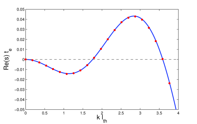
Figure 1: The solid line indicates the real growth rate $s$ of the ballistic transport instability as a function of waveumber $k$, in a homogeneous ring of $\tau_{0}=0.175$ and $\mu=0.025$ (cf. Section 2.2). The solid points indicate the growth rate of the unstable mode that attacks a very low amplitude steady wavetrain with $q=3.5874$, travelling over a background of $\tau_{0}=0.175$ (cf. Section 4).

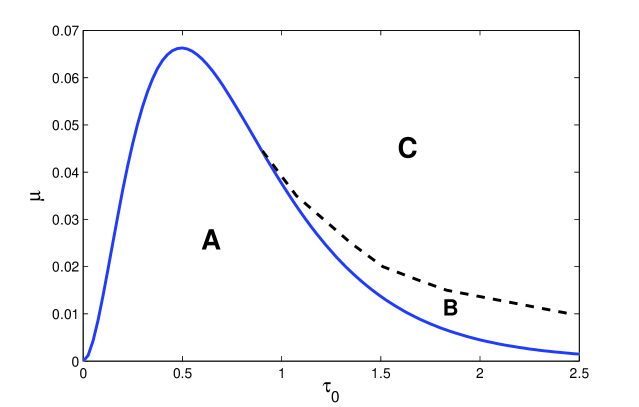
Figure 2: Curves of marginal stability and hysteresis in the $(\tau_{0},\mu)$ plane. Region ‘A’, enclosed by the solid curve, denotes parameter values that are linearly unstable to the BTI. Both regions ‘B’ and ‘C’ are linearly stable. In region ‘B’, however, large-amplitude steady nonlinear wavetrains exist, even though the linear BTI is suppressed.

3 Nonlinear wavetrains

Unstable BTI modes grow exponentially and independently until they leave the linear regime and begin to interact. At this point we are normally obliged to pursue their evolution numerically. Previous work (D92, for example) focussed on how ballistic transport sculpts inner ring edges; it did not directly track the BTI, even if it was sometimes present. Our numerical simulations in Paper 3, in contrast, mostly dispense with ring edges and concentrate explicitly on the BTI’s nonlinear development in isolation. In this paper we explore an alternative approach to both: instead of simulating Eq. (1), we calculate its exact steady nonlinear solutions. These coherent structures, understood as fixed points in the system’s phase space, control the long-time behaviour of the instability, by either repelling or attracting the system’s phase trajectories. As a consequence, they provide insights into the general dynamics and hence the simulation results.

The simplest non-trivial invariant solutions of (1) take the form of steadily travelling wavetrains. Indeed, wavetrains appear in the simulations of D92 for certain parameters. Moreover, the existence of such travelling structures can be anticipated from the mathematical structure of the problem, i.e. its translational symmetry (within the local approximation) and the fact that the onset of instability takes the form of a Hopf bifurcation. Of course, the strongest indication that the BTI supports waves are the observations themselves, with wavetrains permeating the inner B-ring and the C-ring (Horn & Cuzzi 1996, Porco et al. 2005, Colwell et al. 2009).

Though the BTI sustains a rich variety of nonlinear wavetrains, we do not attempt a comprehensive exploration in this paper. To bring out the most relevant results, we restrict the analysis to parameter regimes corresponding to the C-ring and the inner B-ring. Each is treated separately in subsections 3.2 and 3.3, before a more general discussion. First, however, we present our mathematical and numerical approach.

3.1 Nonlinear eigenvalue problem

To calculate travelling solutions to (1) a co-moving spatial co-ordinate $\zeta$ is introduced, defined so that

$$\zeta=x-c_{p}t,$$ (15)

where $c_{p}$ is the phase speed of the wave. To capture wavetrain solutions, we assume $\tau$ is periodic in $\zeta$ with wavelength $\lambda=2\pi/q$, where $q$ is a specified constant wavenumber. As a consequence, Eq. (1) transforms into an ordinary integro-differential equation for $\tau$ in terms of $\zeta$, which we write as

$$c_{p}\partial_{\zeta}\tau+\mathcal{I}-\mathcal{J}+\tfrac{1}{2}\partial_{\zeta}(\mathcal{K}+\mathcal{L})+\mu\,\partial_{\zeta}^{2}\tau=0.$$ (16)

The integral operators in the above can be recast in a straightforward way, keeping the integration limits $\pm\infty$.

Equation (16) describes a nonlinear eigenvalue problem for $\tau$ with eigenvalue $c_{p}$. We must apply periodic boundary conditions, so that $\tau(\zeta+\lambda)=\tau(\zeta)$. An additional constraint is the preservation of a specified mean optical depth $\tau_{0}$, i.e.

$$\tau_{0}=\frac{1}{\lambda}\int_{0}^{\lambda}\tau\,d\zeta.$$ (17)

The three parameters governing the problem are hence $\tau_{0}$, $\mu$, and the wavenumber $q$. Recall that we keep the parameters appearing in our definitions of $R$, $P$, and $f$ constant throughout this paper.

The problem is solved using a Fourier pseudo-spectral method. The domain $0\leq\zeta<\lambda$ is split into $N$ equal components. Typically we set $N=512$, which supplies excellent convergence. The $\zeta$ derivatives in (16) are computed by an excursion into spectral space with a FFT. The $\zeta$ integrals are also evaluated in spectral space, using the convolution theorem. Equations (16) and (17) then become $N+1$ nonlinear equations for $N+1$ unknowns: $c_{p}$ and the values of $\tau$ at the $N$ grid points. These are solved by a multidimensional Newton-Raphson algorithm.

3.2 The C-ring: low amplitude wavetrains

This subsection examines the low-$\tau$ regime relevant to Saturn’s C-ring. We adopt fiducial parameters of $\mu=0.025$ and $\tau_{0}=0.175$. For this choice our numerical method uncovers a family of nonlinear wavetrains of small but non-negligible amplitudes in an interval of $q$ between roughly 1.75 and 3.59. These limiting values coincide with the wavenumbers of the two marginal linear modes for which Re($s)=0$, as shown in Fig. 1. Thus the marginal linear modes bracket the wavelengths of allowed nonlinear waves.

We measure the amplitudes of the wavetrains with $\text{max}(\tau)-\tau_{0}$. In the left panel of Fig. 3 we plot the amplitude as a function of $q$. Its maximum value is a little less than $0.2$ and occurs for $q\approx 2.54$, less than the wavenumber of fastest linear growth, which is closer to 2.84. In the second panel the solid curve represents the corresponding phase speeds $c_{p}$. Interestingly, the $q$ at which $c_{p}=0$ is approximately that which yields the largest wave amplitude. Superimposed, as data points, are the wavespeeds of the linear BTI modes. The two curves are very similar, sharing the same values at the endpoints of the $q$ interval. Finally, the group velocity, $c_{g}=d(qc_{p})/dq$, is negative for all permitted $q$: information always travels inwards. This is true even for longer waves for which the wave crests, in contrast, travel outwards ($c_{p}>0$). Generally $|c_{g}|>|c_{p}|$ and varies between -0.192 and -1.13, with the longest waves possessing the slowest group velocities.

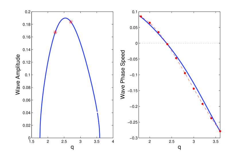
Figure 3: Solid curves correspond to the amplitudes and phase speeds $c_{p}$ of nonlinear wavetrains as functions of wavenumber $q$ for C-ring parameters: $\tau_{0}=0.175$ and $\mu=0.025$. In the second plot the wavespeeds of the linear BT modes are also plotted as data points joined by a dashed curve. Wavetrains between the two asterisks in the first panel are linearly stable (cf. Section 4).

In Fig. 4 we present two representative wavetrain profiles. The top panel corresponds to a comparatively large-amplitude wave with $q=2.615$. The variation in $\tau$ between peak and trough is roughly 0.2, similar to what is observed in the C-ring. We plot a comparatively low-amplitude wave in the lower panel with a shorter wavelength. Here $q=3.550$, meaning the wavetrain is very near the limiting $q$ beyond which no solutions exist. As a consequence, it is essentially the same as the marginal (and steady) linear BTI mode, and thus exhibits a sinusoidal profile.

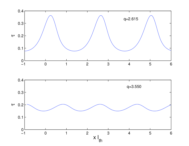
Figure 4: Profiles of two wavetrains corresponding to $q=2.615$ (top panel) and $q=3.550$ (bottom panel). The mean optical depth $\tau_{0}$ is $0.175$ and $\mu=0.025$.

These results suggest that the BTI when near marginality, as it is in the C-ring, tends to saturate in low-amplitude travelling waves. These wavetrains possess a wavelength $\lambda$ between approximately 1.5 and 3 throw lengths $l_{\text{th}}$, values which also bracket the set of unstable linear modes. Given their general sinusoidal appearance and the fair correspondence between the linear and nonlinear wave speeds (Fig. 3b), they invite a weakly nonlinear analysis, which yields their saturation amplitudes analytically. The calculation is outlined in Section 5 and the Appendix. There it is also shown that, in addition to wavetrain solutions, there also exist solutions that consist of long travelling modulations of these same wavetrains.

Our solutions probably correspond to the ‘ripples’ that appear in low-$\tau$ regions in some D92 simulations. Though those authors conjecture that the waves are driven by the B-ring edge, they also leave open the idea that they could be generated by an instability working in isolation, which is what we show here.

Because the characteristic throw length $l_{\text{th}}$ is poorly constrained, it is difficult to unambiguously compare ballistic transport results with the observed features in the C-ring. Do our solutions correspond to the 100-km plateaus or the 1000-km undulations? Given the two markedly different lengthscales of these features, and the fact that they can occur at the same radii, it is unlikely that the BTI generates both concurrently. We associate the BTI with the 1000-km undulations. The general morphology of the theoretical profiles (low amplitude and generally sinusoidal) bears a closer resemblance to the long undulations than to the plateaus and their characteristic ‘flat-top’ profile. A consequence of this identification is that $l_{\text{th}}\sim 500$ km, at least in the C-ring.

3.3 The B-ring: hysteresis

In this subsection we adopt a parameter regime corresponding to the inner B-ring. We take $\mu=0.025$ again and set $\tau_{0}=1.3$. This choice is suitable for a situation amidst a ‘wavy’ zone, rather than a ‘flat’ zone, in which the mean optical depth is slightly less (Colwell et al. 2009).

For these parameters the linear theory states there are no growing modes. The BTI is extinguished because the homogeneous state is too optically thick. When $\mu=0.025$, the largest $\tau_{0}$ that supports instability is $\tau_{0}\approx 1.2$. Nevertheless, we are able to compute wavetrain solutions of non-trivial amplitudes. Similarly to lower $\tau_{0}$, they occur in a finite interval of wavenumber: $q$ must lie between approximately 2 and 3. Moreover, we find two distinct families of solutions. For fixed $q$ there exist two wavetrains of differing amplitude and morphology. Note that as the stable homogeneous state $\tau=1.3$ is also a solution for these parameters, the system is potentially bistable.

The solution branches are plotted in the left panel of Fig. 5 as functions of wavenumber $q$. The right panel shows the associated phase speeds $c_{p}$. The solid line indicates the upper branch of solutions, and the dashed line describes the lower branch. Taken together the two families form an ‘isola’ in the solution space. Unlike the low $\tau_{0}$ case explored earlier, the amplitudes of the wavetrains are large, and the wavecrests propagate inwards, albeit extremely slowly. For fiducial values of $l_{\text{th}}$ and $t_{e}$, the phase speed lies between 1 and 100 mm/yr. We certainly expect no measurable difference in the wave positions since the first Voyager images of the B-ring. The group velocity $c_{g}$, though typically negative, can take positive values near the upper and lower limits of permitted $q$.

In Fig. 6 we present two examples of the solutions’ profiles. The top panel corresponds to a wavetrain from the upper wave branch, and the bottom panel from the lower branch. Note that $\tau$ in the upper branch waves varies between roughly 0.4 and 2.3, from trough to peak. In contrast, the lower branch exhibits a more narrow variation. Both profiles deviate appreciably from the sinusoidal shapes of the low-$\tau_{0}$ solutions of Section 3.2. The upper branch solution exhibits slight ‘ramp-like’ features to the right of its minima, a feature that becomes more evident at larger wave amplitude (see next subsection). The morphology of the upper branch matches fairly well with those produced by Durisen et al.’s simulations of the inner B-ring edge (D92); see for example their Fig. 6. Consequently, we regard the D92 waves as direct analogues of our solutions.

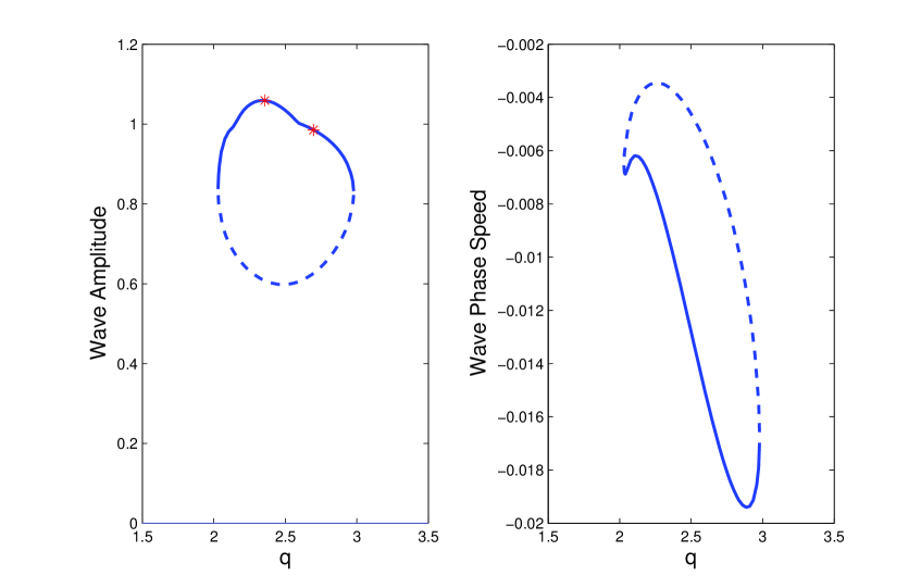
Figure 5: The amplitudes and phase speeds $c_{p}$ of wavetrain solutions as functions of wavenumber $q$ for parameters corresponding to the inner B-ring: $\tau_{0}=1.3$ and $\mu=0.025$. There are two branches of wave solutions which we distinguish by solid and dashed lines. In addition, the homogeneous state $\tau=1.3$ is also a solution. Upper branch solutions lying between the two asterisks are linearly stable. All the members of the lower branch are unstable (cf. Section 4). There also exists a very narrow band of stable upper branch solutions near $q=2.04$ which is not indicated by asterisks.

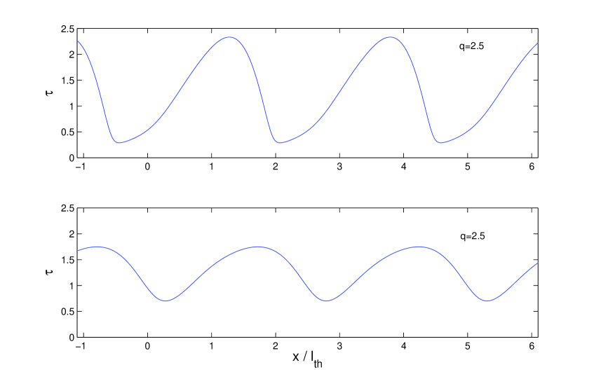
Figure 6: Two representative examples of wavetrain solutions for $\tau_{0}=1.3$ and the same wavenumber $q=2.5$. The top panel shows the stable wavetrain from the upper branch of solutions, while the bottom panel shows the unstable one from the lower branch.

From the structure of the solution space, we anticipate that the lower wave branch is linearly unstable. The system will prefer to migrate to either the ‘flat’ homogeneous state or one of the upper ‘wave’ states. We show this in some detail in Section 4. This, however, causes trouble when we compare the morphologies of the stable upper-branch waves with the observed waves in the inner B-ring. As mentioned, the former exhibit very deep troughs ($\tau\sim 0.4$) and large peaks ($\tau\sim 2.3$), while the latter’s optical depth variation is less marked, with $\tau$ ranging between roughly 0.8 and 1.9 (Colwell et al. 2009). Inconveniently, the unstable lower branch waves offer a much better fit! Of course, our theoretical profiles are framed in terms of dynamical optical depth, while the Cassini cameras measure photometric optical depth, and the likely presence of self-gravity wakes ensures the two quantities differ. It is unclear, though, if this can fully account for the discrepancy: obviously, further work is needed. Finally, it is worth mentioning that the more detailed Durisen et al. calculations also share the same deep troughs (D92), and so it is unlikely that the disagreement arises because of idealisations in our model.

Because two stable states are possible at any given location the spatial domain may split up into ‘flat’ and ‘wave’ zones, each separated by a ‘front’ that may itself move, but at a speed different from $c_{p}$. Such a partitioning is indeed what the observations show. In principle, it is possible to analytically explore families of such ‘homoclinic’ structures (Burke and Knobloch 2007). Unfortunately our system exhibits wave zones that spread as well as travel, and as a consequence are difficult to work with. They are more easily treated via numerical simulations, and we show detailed examples in Paper 3.

3.4 General structure of solution space

Having examined two representative examples in detail, we now summarise the general solution structure as $\tau_{0}$ and $\mu$ vary, in addition to the wavenumber $q$. We, however, give slightly more emphasis to the $\tau_{0}$ dependence because the solutions’ $\mu$ dependence is less interesting.

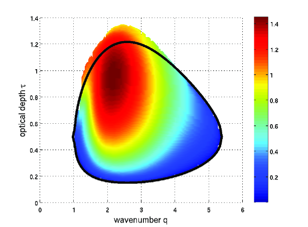
Figure 7: The amplitude of wavetrain solutions as a function of $\tau_{0}$ and $q$ for fixed $\mu=0.025$. White regions indicate that no wave solutions exist. The thick black line encompasses the region in parameter space that is linearly unstable. As wave solutions exist in regions that are linearly stable the system exhibits hysteresis. In bistable regions only the amplitude of the upper wave branch is plotted.

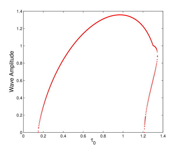
Figure 8: The wave amplitude as a function of $\tau_{0}$ for fixed $q=2.5$ and $\mu=0.025$. Both upper and lower wave branches are included. Between roughly $\tau_{0}=1.2$ and $1.35$ the system exhibits hysteresis.

Figure 7 presents coloured contours of the wave amplitude as a function of $q$ and $\tau_{0}$, with $\mu=0.025$. The white area indicates where no wave solutions exist. The thick black curve encompasses the region within which linear modes grow. For most values of $\tau_{0}$ and $q$, wave solutions are confined within the linear curve. But when $\tau_{0}$ is larger there exist solutions for parameters where the homogeneous state is stable. These regions exhibit bistability and admit two wave solutions with different amplitudes (as in Section 3.3), though we only plot the upper branch amplitudes in Fig. 7.

The maximum amplitude for a given $\tau_{0}$ always occurs at a $q$ smaller than that of the fastest growing linear mode. Furthermore, the $q$ that yields the maximum amplitude and the $q$ that gives $c_{p}=0$ are relatively close to each other. For example, at $\tau_{0}=1$, the former $q$ is $2.18$ and the latter is $2.32$, while the fastest growing linear mode possesses $q=3.02$. When $\tau=0.5$, the largest amplitude occurs at $q=2.12$, while $c_{p}=0$ occurs at $q=2.42$, and the fastest growing mode has $q=3.45$.

Near $\tau_{0}\approx 0.9$ and for $q\approx 1.3$ the solution surface is complicated and appears to ‘tear’, with nearby regions twisting upwards to either larger amplitudes or downwards to zero amplitude. This suggests there may be additional solution branches. We have not attempted to compute these additional (hypothetical) longer wavelength structures, and have not observed them in the simulations of Paper 3.

In Fig. 8 we plot the wave amplitude as a function of $\tau_{0}$, keeping both $q$ and $\mu$ constant. Both upper and lower solution branches are included and thus the figure clearly represents the hysteresis at larger $\tau_{0}$. When $\mu=0.025$, hysteresis occurs in a relatively small region in parameter space, between roughly $\tau_{0}=1.2$ and 1.35. Notable is the large amplitude of the upper wave state; this could mean that large disturbances are needed to transfer a portion of ring from the flat state to the wave state and vice versa. Perhaps the Janus/Epimetheus 2:1 inner Lindblad resonance, which falls within a wave region in the inner B-ring, could provide such a strong disturbance (Colwell et al. 2009).

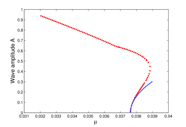
Figure 9: The red points represent the numerically computed amplitude as a function of $\mu$ for fixed $q=2.57453$ and $\tau_{0}=1$. Both upper and lower wave branches are included. The solid blue line represents amplitudes calculated from the weakly nonlinear analysis of Section 5 and the Appendix.

We explore the dependence of the solutions on $\mu$ in Fig. 9. There we plot amplitude versus $\mu$ while keeping $\tau_{0}$ and $q$ constant. Hysteresis is also observed near the critical $\mu$, but only at larger $\tau_{0}$, not at lower $\tau_{0}$. We also plot the amplitude computed from the weakly nonlinear analysis of the Appendix, namely Equation (83). This solution is discussed in Section 5.

Lastly, we examine hysteresis in the $\tau_{0}$—$\mu$ plane. In Figure 2, it is localised to Region ‘B’. The dashed curve is achieved by optimising the critical $\tau$ upon which the solution branches terminate, as $q$ varies but $\mu$ remains fixed. As is clear from the plot, hysteresis only occurs for higher optical depths, approximately $\tau>1$. But what is striking is how far the nonlinear solutions survive into the linearly stable high-$\tau$ regime. For $\mu=0.01$, the linear stability shuts down at $\tau_{0}=1.64$, but nonlinear waves persist up to $\tau_{0}=2.45$. For smaller $\mu$, BTI wavetrains occur at extremely large optical depths indeed. It is improbable, however, that the central and outer B-ring — the only venues exhibiting such high $\tau$ — possess $\mu<0.01$ (see discussion in Paper 1). Consequently, the linear or nonlinear BTI should not play a role there.

Figure 10: Two waveforms for $\tau_{0}=1$ and $\mu=0.025$. The top panel shows a wave possessing $q=2.4699$ and the lower panel a longer wave with $q=1.2824$.

Before moving on, we show two additional waveforms from different locations in Fig. 7. The upper panel of Fig. 10 shows the largest amplitude wavetrain possible, occurring for $\tau_{0}=1$ and $q\approx 2.47$. Its general morphology is similar to Fig. 6a, but it exhibits longer and deeper troughs, with $\tau$ dipping below $0.2$, as well as more conspicuous ramp features. In the lower panel we plot a long wavelength wavetrain from the region to the left of the dark line in Fig. 7 at $\tau_{0}=1$. This wave possesses $q\approx 1.28$. Its morphology is striking, consisting of a trough, plateau, and peak. Though interesting, it is difficult to connect this waveform with observations. Moreover, as we find in Section 4, such long wavelength waves are unstable and unlikely to play a role in the main dynamics.

4 Linear stability

Of all the previously computed wavetrains we expect the linearly stable ones to dominate the BTI’s nonlinear evolution. Linearly stable solutions serve as attractors in the system’s phase space: the ring is likely to settle on or around them, and hence exhibit their chief characteristics. In this section we determine the stability of the solutions computed in Section 3. Our main result is that, of all the various wavetrain solutions available, only a small subset are actually stable. For given $\tau_{0}$ and $\mu$, stable wavetrains usually occur on a narrow band of $q$ encompassing the values that yield $c_{p}=0$ and the maximum wave amplitude.

4.1 Modal analysis

First we set up the mathematical framework with which to determine stability. The underlying wavetrain is denoted, as before, by $\tau$ and a small perturbation on top of this solution by $\tau^{\prime}$. The system is transferred to a comoving coordinate system with spatial variable $\zeta$, as defined in Eq. (15). Once we approximate (1) for small $\tau^{\prime}$, we obtain a linear equation for $\tau^{\prime}$ in $t$ and $\zeta$ that is $\lambda$-periodic in $\zeta$. As a consequence, we make the Floquet ansatz and let $\tau^{\prime}$ take the following form:

$$\tau^{\prime}=\text{e}^{st+\text{i}k\zeta}\,\hat{\tau}(\zeta),$$ (18)

where $s$ is a (complex) growth rate, $k$ is the (real) wavenumber of the disturbance envelope, the Floquet exponent, and $\hat{\tau}$ is a $\lambda$-periodic function in $\zeta$. Recall that $\lambda=2\pi/q$. Generally, $s$ and $k$ differ from the linear growth rates that appear in Section 2.2, though in the limit in which the wavetrain amplitude $\to 0$ they do coincide. We need only examine values of $k$ between 0 and $q/2$; outside this range the solutions repeat.

The governing linearised equation for $\hat{\tau}$ is

$$s\,\hat{\tau} =\mathcal{I}^{\prime}-\mathcal{J}^{\prime}+\tfrac{1}{2}\left(\partial_{\zeta}+\text{i}k\right)\left[\mathcal{K}^{\prime}+\mathcal{L}^{\prime}\right]$$

$$\hskip 85.35826pt+\mu\left(\partial_{\zeta}^{2}+2\text{i}k\partial_{\zeta}-k^{2}\right)\hat{\tau}.$$ (19)

Using periodic summation, the four primed integral operators can be manipulated into the following forms, which are better suited to our numerical method:

$$\mathcal{I}^{\prime} =P^{\prime}(\zeta)\,\hat{\tau}(\zeta)\,\int_{0}^{\lambda}R(\zeta-\xi)f_{\Sigma}(0,\xi)\,d\xi$$

$$\hskip 28.45274pt+P(\zeta)\int_{0}^{\lambda}R^{\prime}(\zeta-\xi)\,\hat{\tau}(\zeta-\xi)\,f_{\Sigma}(k,\xi)\,d\xi,$$ (20)

$$\mathcal{J}^{\prime} =R^{\prime}(\zeta)\,\hat{\tau}(\zeta)\,\int_{0}^{\lambda}P(\zeta+\xi)f_{\Sigma}(0,\xi)\,d\xi$$

$$\hskip 28.45274pt+R(\zeta)\int_{0}^{\lambda}P^{\prime}(\zeta+\xi)\,\hat{\tau}(\zeta+\xi)\,f_{\Sigma}(-k,\xi)\,d\xi,$$ (21)

$$\mathcal{K}^{\prime} =-P^{\prime}(\zeta)\,\hat{\tau}(\zeta)\,\int_{0}^{\lambda}R(\zeta-\xi)\partial_{k}f_{\Sigma}(0,\xi)\,d\xi$$

$$\hskip 19.91684pt-P(\zeta)\int_{0}^{\lambda}R^{\prime}(\zeta-\xi)\,\hat{\tau}(\zeta-\xi)\,\partial_{k}f_{\Sigma}(k,\xi)\,d\xi,$$ (22)

$$\mathcal{L}^{\prime} =R^{\prime}(\zeta)\,\hat{\tau}(\zeta)\,\int_{0}^{\lambda}P(\zeta+\xi)\partial_{k}f_{\Sigma}(0,\xi)\,d\xi$$

$$\hskip 19.91684pt+R(\zeta)\int_{0}^{\lambda}P^{\prime}(\zeta+\xi)\,\hat{\tau}(\zeta+\xi)\,\partial_{k}f_{\Sigma}(-k,\xi)\,d\xi.$$ (23)

To ease the notation in the above, we have set $P(\zeta)=P[\tau(\zeta)]$, $P(\zeta-\xi)=P[\tau(\zeta-\xi)]$, $P^{\prime}(\zeta)=P^{\prime}[\tau(\zeta)]$, etc. We have also introduced the $\lambda$-periodic distribution function $f_{\Sigma}$, defined via

$$f_{\Sigma}(k,\xi)=\sum_{n=-\infty}^{\infty}\text{e}^{-\text{i}k(\xi+\lambda n)}f\left(\xi+\lambda n\right).$$ (24)

For the off-centred Gaussian profile of Eq. (10), the new distribution function can be re-expressed as

$$f_{\Sigma}=\frac{1}{2\pi}\text{e}^{-\text{i}\xi_{0}k-\frac{1}{2}d^{2}k^{2}}\Theta_{3}\left(\tfrac{1}{2}\text{i}k/q+\tfrac{1}{2}q(\xi-\xi_{0}),\,\text{e}^{-\frac{1}{2}d^{2}q^{2}}\right),$$

where $\Theta_{n}$ is the Jacobi theta function (Whitaker and Watson 1990). However, given the rapid convergence of the series in (24), it is more convenient in practice to use a truncated series expression for $f_{\Sigma}$.

Equation (19) is a linear eigenvalue problem for $\hat{\tau}$ with eigenvalue $s$. The main parameters comprise $\tau_{0}$, $\mu$, and $q$, which specify the nonlinear wavetrain whose stability we test, and $k$ the wavenumber of the linear mode attacking the wavetrain.

Because there are multiple modes that are potentially unstable we seek a numerical method that can retrieve more than one eigensolution at a time. We hence transform (19) into an algebraic eigenvalue problem by approximating the operator on the right side of the equation as a matrix. The variable $\zeta$ is discretised on the domain $[0,\,\lambda]$ into $N$ equally spaced points, and the spatial derivatives are represented by pseudo-spectral matrices (see Boyd 2002). We approximate by quadrature formulae the integrals with $\hat{\tau}$ in the integrand. Because the integrands are periodic, the trapezoidal rule offers spectral accuracy. We may write such integrals as finite sums, and hence as matrices operating on the discretised $\hat{\tau}$. Once the operator on the right side of (19) is reduced to an $N$-by-$N$ matrix, we extract the eigenvalues and eigenvectors using either the QR algorithm or an Arnoldi method (Golub and van Loan 1996).

4.2 Numerical results

We do not give an exhaustive stability analysis of all wave solutions; instead we focus on the wavetrains associated with the C-ring and B-ring, as explored in Sections 3.2 and 3.3.

We first check the stability of extremely low amplitude wavetrains, when the wavetrain amplitude approaches 0. Unstable modes in this limit should coincide with the BTI modes that attack the homogeneous state, as detailed in Section 2.2. This provides a useful numerical check on our eigensolver. In Fig. 1 we plot, with red dots, the growth rate of the unstable mode that attacks a short-wavelength low-amplitude wavetrain with $q=3.5724$, when $\tau_{0}=0.175$ and $\mu=0.025$. This wave possesses an amplitude of $8.7\times 10^{-3}$. The solid line is the growth rate computed from the linear theory of the homogeneous state. The agreement is excellent and thus verifies our mathematical and numerical apparatus.

When the wavetrain amplitude becomes larger the dispersion relation deviates from that of the homogeneous case in Fig. 1. Ultimately, more than one mode can possess a positive growth rate as $k$ varies. In Fig. 11, examples of growing modes for two different wavetrains are shown for a low $\tau_{0}$ ring. The top panel describes the sole growing mode that attacks a shorter wavelength wave. The bottom panel presents two potentially growing modes that destabilise a longer wave. Other wavetrains support similarly complicated dispersion relations, which we need not go into the details of. It is important to note that there is always a neutral mode $s=0$ when $k=0$. It is linked to the translational invariance of our model.

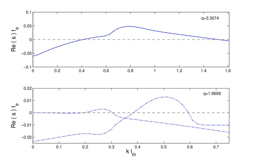
Figure 11: The dependence on wavenumber $k$ of the growth rates $s$ of secondary modes attacking two wavetrains. In both cases $\tau_{0}=0.2$ and $\mu=0.025$. The top panel is associated with a wavetrain with $q=3.3074$, the bottom panel with a wavetrain with $q=1.9699$. Note that the longer wave supports two growing modes.

Of more interest is a stability criterion in terms of $q$, for given $\tau_{0}$ and $\mu$. Essentially, which wavetrains are stable and which are not? In general, in a given family of wavetrains we find that both its shortest and longest members are unstable. At low $\tau_{0}$ this is expected: wavetrains near the upper and lower critical $q$’s have low amplitudes and thus will have similar stability properties to the (unstable) homogeneous state — cf. Fig. 3a. It is interesting that this is also the case for larger $\tau_{0}$ solutions, which can have large amplitudes at lower $q$.

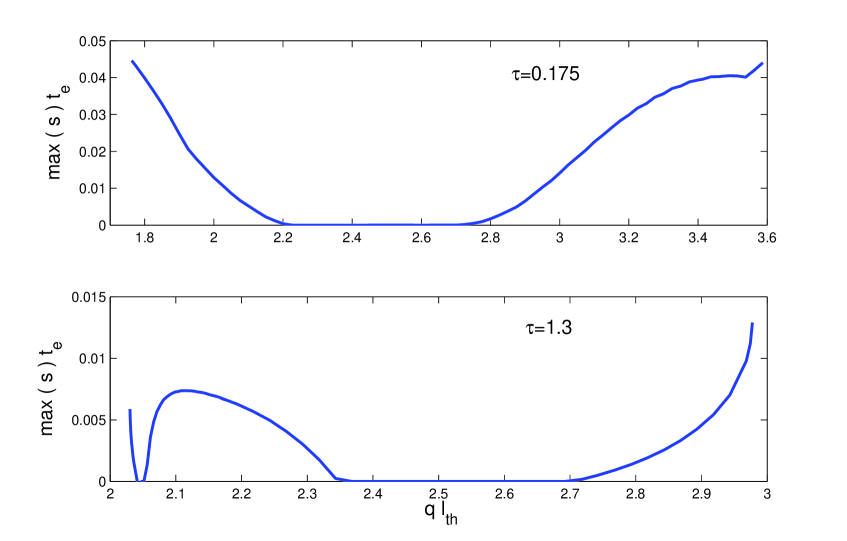
Figure 12: The maximum growth rate $s$ of the secondary instability as a function of the wavenumber $q$ of the underlying wavetrain. The first panel deals with wavetrains possessing $\tau_{0}=0.175$, and the second panel deals with upper-branch wavetrains possessing $\tau_{0}=1.3$. The ballistic Prandtl number is held fixed at $\mu=0.025$. When max($s$)$\leq 0$ the wavetrain is stable.

For our fiducial C-ring parameters of Section 3.2, only wavetrains with $2.225<q<2.705$ are linearly stable. This result is illustrated in the first panel of Fig. 12, which shows the growth rate $s$, maximised over $k$, as a function of wavetrain wavenumber $q$. We have stability when the curve takes values equal or less than 0. The stable band of wavenumbers encompasses waves with the largest amplitude and slowest wavespeed (see Fig. 3), a result that may have been anticipated. The most nonlinear solution will most effectively distort the background equilibrium state and hence mitigate the conditions favourable for BTI.

Note that the fastest growing linear BTI mode possesses a wavenumber ($q=2.84$) outside this narrow range. This mode will dominate all others in the initial phase of a ring’s evolution, and probably saturates by forming a nonlinear wavetrain of the same wavenumber. Being an unstable solution, however, the system eventually migrates away and probably undergoes a wavelength selection process as it seeks the stable set of solutions. Similar behaviour is witnessed during the saturation of the viscous overstability, with the ring hopping from one unstable solution to another until it finds a stable wavetrain (Latter & Ogilvie 2009, 2010).

For B-ring parameters with $\tau_{0}=1.3$ we find that the lower branch of solutions in Section 3.3 is unstable for all $q$. These waves are destabilised by a fast growing $k=0$ mode that seems to bear little resemblance to the classical BTI of the homogeneous state. The upper branch, however, possesses a band of stable solutions for $2.356<q<2.698$, which includes the waves with larger amplitudes (see Fig. 5). But there is also an unusual much narrower band of stable states around $q=2.05$. These results are summarised in the second panel of Fig. 12.

Overall this stability behaviour is reflected at other $\tau_{0}$. Almost always, stable solutions exist in a narrow band of $q$ bracketing the largest amplitude waves.

5 Dynamics of long and slow modulations

So far we have uncovered the invariant fixed points of the BTI dynamical system, i.e. steadily travelling wavetrains. These should control its nonlinear evolution, and we check exactly how in Paper 3 with numerical simulations. But it is possible to obtain an analytic handle on the full time-dependent dynamics in certain relevant limits, especially near marginal stability. Here we derive reduced equations for the long and slow dynamics of the waves’ modulations by exploiting the separation of scales between the modulations and their carrier waves. We find that the modulations of low-amplitude wavetrains are governed by the complex Ginzburg-Landau equation (CGLE), which is a partial differential equation that describes generic nonlinear wave phenomena in diverse settings (Aranson and Kramer 2002). The mathematical derivation is located in the Appendix, in this section we briefly summarise its main points and implications for the C-ring.

We select a point on the curve of marginal linear stability described in Fig. 2 in the parameter space of $(\tau_{0},\mu)$. Next we move off the stability curve, either by slightly perturbing $\mu$ or $\tau_{0}$. In the Appendix, we choose $\mu$ as it simplifies the mathematics somewhat. The perturbation’s proximity to marginality is quantified by the small dimensionless parameter $\epsilon$. It also serves to separate the scales of the (fast) underlying waves and the (slow) modulations. The former depend only on the short space and time variables of $x$ and $t$, while the latter depend only on the long space and time variables $X\sim\epsilon x$ and $T\sim\epsilon^{2}t$. In this limit, to leading order, the solution behaves as

$$\tau=\tau_{0}+A(X,\,T)\text{e}^{\text{i}k_{c}x-\text{i}\omega_{c}t}+\text{c.c.},$$ (25)

where $k_{c}$ and $\omega_{c}$ are the wavenumber and frequency of the marginal linear mode, $A$ is the complex-valued wavetrain amplitude, and ‘c.c.’ indicates the complex conjugate. The amplitude $A$ describes the modulations and obeys a version of the CGLE,

$$\partial_{T}A=\lambda A+\beta\,|A|^{2}A+\kappa\,\partial_{X}^{2}A,$$ (26)

where $\beta$ and $\kappa$ are (complex) constants, and $\lambda$ is a control parameter. In the Appendix we give expressions for $\beta$ and $\kappa$ in terms of the various parameters of the ring.

The set of solutions to Eq. (26) includes steady homogeneous solutions in which $A$ is a constant; these connect to the solutions computed in Section 3. But the CGLE also admits plane waves with $A\propto\text{exp}(\text{i}k_{m}X-\text{i}\omega_{m}T)$, where $k_{m}$ and $\omega_{m}$ are the wavenumber and frequency of long modulations. Some or all of these solutions may be unstable, in which case various time-dependent behaviours can emerge, including the aperiodic emergence and destruction of strong inhomogeneities in the carrier wavetrain (wherein its phase jumps abruptly) as well as low-level chaotic variations in the waves’ amplitude (Aranson and Kramer 2002). It is likely that low amplitude undulations in the C-ring could undergo some subset of these dynamics.

For the moment, we use (25) and (26) to compute steady wavetrains with no modulations in order to compare with some of the results in Section 3. In Figure 9 the solid curve represents the real wave amplitude from the nonlinear analysis in the Appendix, cf. Eqs (83)-(84). As expected, the agreement is good at low amplitudes, but the two solutions deviate as the lower branch curves upwards towards the saddle-node.

6 Discussion

In this final section we summarise our results and apply them to the observational problems of Saturn’s B- and C-rings. We also point towards future work.

First, we have shown that the BTI can saturate via the formation of steadily travelling nonlinear wavetrains. Near marginal stability at low $\tau$, these solutions inhabit an interval of intermediate wavenumber $q$. For example, when the mean optical depth $\tau_{0}=0.175$, wavetrains exist with a $q$ between 1.75 and 3.59 (in units of $1/l_{\text{th}}$). The amplitudes of these waves are relatively small, with $\tau$ varying by $\sim 0.1$ between peaks and troughs (cf. Fig. 4). For the most part, these solutions are close to sinusoidal in appearance and possess phase speeds approximately equal to the linear BTI modes (Fig. 3).

On the other hand, at large $\tau$ the system permits hysteresis: even if a homogeneous ring is linearly stable it can still support large-amplitude wavetrain solutions via the ballistic transport mechanism. Consequently, the ring will want to evolve to either the flat homogeneous state, or a stable wave state. The wavetrains do not resemble sinusoids, and the peak to trough variation is large, varying between 1 and 1.6 in $\tau$ (Fig. 6). Wavecrests in this marginal high-$\tau$ parameter regime propagate extremely slowly, at most with a phase speed $\sim 0.01\,l_{\text{th}}/t_{e}$ or 1-100 mm yr^-1 (see Fig. 5).

We tested the linear stability of these structures and found that for given parameters only a subset of the wavetrain solutions are stable. Generally, stable solutions possess the greatest amplitude and propagate the slowest. It is likely that the system will select one of these solutions if left to freely evolve. We also demonstrate that low-amplitude wavetrains undergo large-scale modulations which are governed by the complex Ginzburg-Landau equation. The amplitudes of our C-ring waves may then share in its interesting, sometimes disordered, dynamics.

These results are compatible with observations of B- and C-ring structure (Porco et al. 2005, Colwell et al. 2009), as well as previous simulations of the inner B-ring (D92). Turning to the B-ring first, it is likely that the observed adjoining flat and wave zones between 93,000 and 98,000 km (Fig. 13.13 in Colwell et al. 2009) are products of the hysteresis exhibited by our model. The flat regions correspond to where the ring has fallen into the stable homogeneous state, and the wave regions to where it has jumped into the stable wave state. These zones are connected by fronts, which should exhibit additional dynamics that time-dependent simulations may probe. Perturbations that may have thrust B-ring regions out of the homogeneous state’s basin of attraction might include the inner B-ring edge, the transition to extremely large $\tau$ at $r=99,000$ km, or the Janus/Epimetheus 2:1 inner Lindblad resonance.

There are two problems that this scenario faces. First is the deepness of the troughs in the theoretical wave profiles. Typically the theoretical troughs possess a dynamical optical depth of $\sim 0.4$. Meanwhile in the B-ring the troughs yield a photometric optical depth of $\sim 0.8$. It is true that self-gravity wakes complicate the relationship between dynamical and photometric optical depth, yet the discrepancy is concerning. Second, is the observed mean optical depth differs in the wave and in the flat zones: in the former it is approximately 0.8; in the latter is is closer to 1.3. This further complicates the mapping of our results to the observations, and indicates our theory requires additional refinement.

Comparison of our solutions to C-ring observations must first resolve one key question: does the free evolution of the BTI generate the low-amplitude 1000-km undulations, found between 77,000 km and 86,000 km, or the larger-amplitude 100-km plateaus, between 84,000 and 91,000 km (Fig. 13.17 in Colwell et al. 2009)? On account of the small amplitudes and morphology of our wavetrain solutions, we conclude that the 1000-km undulations are the result of the BTI working alone. The plateaus are probably caused by something else, though the ballistic transport process may influence their general shape (Estrada & Durisen 2010).

If both the 1000-km undulations in the C-ring and the 100-km waves in the B-ring are BTI wavetrains then it follows that $l_{\text{th}}$ could vary significantly between the two radial locations. This variation may arise from differences in the sizes, composition, or regolith properties of the ring particles, on the one hand, or the trajectories and speeds of the incoming meteoroids, on the other. For example, recent spectroscopic studies indicate that the sizes of regolith grains vary with radius (Morishima et al. 2012, Hedman et al. 2013). But it is unclear whether this means particles are more or less ‘fluffy’ (and hence $l_{\text{th}}$ smaller or greater) in different ring regions. We view this as a key question in the study of ballistic transport, deserving of further study.

In our following paper, the role of these invariant solutions is made clear through full time-dependent simulations. There we also run a suite of simulations of the inner B-ring edge, which itself could be unstable to the BTI. Further work will improve our basic model, through the addition of more physical processes. For instance, the ring’s viscosity should be an increasing function of $\tau$, not a constant as assumed here. Preliminary results, however, show no qualitative changes arises from this effect. Of greater importance may be the form of the absorption probability, $P$. Throughout this paper, we assume it only depends on the absorbing radius. But in lower optical depth regions it will also depend on the ejecta emitting radius. This effect will influence both the B and C-rings, the former on account of the low $\tau$ achieved in wavetrain troughs.

Appendix A Weakly nonlinear analysis

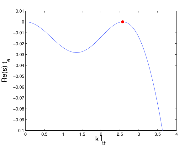
Figure 13: The linear dispersion relation of the BTI for a marginal case. Here the example is taken of $\tau=1$ and $\mu=0.0376287$. The critical $k$ in this situation is $k=2.57$, which is illustrated with a red dot.

A.1 Critical state

We first define the critical state for which the BT instability has zero growth rate for non-zero $k$. In Fig. 13 we plot the dispersion relation of the BTI at marginality when $\tau_{0}=1$ and $\mu\approx 0.0376$. Formally, a general marginal state is defined via

$$\text{Re}(s)=0,\qquad\text{Re}\left(\frac{ds}{dk}\right)=0.$$ (27)

We set $\tau_{0}$ as a free parameter, and solve these two equations for the critical $\mu$ and $k$, hence denoted by $\mu_{c}$ and $k_{c}$. A linear mode with the latter wavenumber has zero growth rate but non-zero wave frequency $\omega_{c}=\omega(k_{c})$. We define the linear wave frequency to be $\omega=-\text{Im}(s)$. The phase speed is hence $c_{p}=\omega_{c}/k_{c}$ and its group velocity is $c_{g}=(d\omega/dk)_{c}$.

A.2 Slow variables and expansions

We introduce the small dimensionless parameter $\epsilon$, so that $0<\epsilon\ll 1$. The critical $\mu$ is then perturbed very slightly so that

$$\mu=\mu_{c}-\epsilon^{2}\lambda/k_{c}^{2},$$ (28)

where $\lambda$ is a control parameter describing the proximity of the ring to marginality. When $\lambda<0$ the system is subcritical, and when it is $>0$ the system is supercritical. Next we consider the long space and slow time variables

$$X=\epsilon(x-c_{g}t),\qquad T=\epsilon^{2}t.$$ (29)

If $\tau$ depends independently on $x$, $t$, $X$, and $T$, we may replace the partial derivatives in our governing equation as follows:

$$\partial_{x}\to\partial_{x}+\epsilon\,\partial_{X},\qquad\partial_{t}\to\partial_{t}-\epsilon\,c_{g}\,\partial_{X}+\epsilon^{2}\partial_{T}.$$ (30)

We expand $\tau$ in small $\epsilon$ around the reference optical depth $\tau_{0}$:

$$\tau=\tau_{0}+\epsilon\,\tau_{1}+\epsilon^{2}\,\tau_{2}+\epsilon^{3}\,\tau_{3}+\dots.$$ (31)

Correspondingly we expand both $R$ and $P$, obtaining

$$P =P_{0}+\epsilon\,P_{0}^{\prime}\,\tau_{1}+\epsilon^{2}\left(P_{0}^{\prime}\tau_{2}+\tfrac{1}{2}P_{0}^{\prime\prime}\tau_{1}^{2}\right)$$

$$\hskip 28.45274pt\epsilon^{3}\left(P_{0}^{\prime}\tau_{3}+P_{0}^{\prime\prime}\tau_{1}\tau_{2}+\tfrac{1}{6}P_{0}^{\prime\prime\prime}\tau_{1}^{3}\right)+\dots,$$ (32)

where the subscript $0$ indicates evaluation at $\tau=\tau_{0}$ and a prime indicates differentiation with respect to $\tau$. An analogous expression exists for $R$.

A.2.1 Direct mass transfer integrals

Consider first the integral operator

$$\mathcal{I}=P[\tau(x)]\,\int R[\tau(x-\xi)]\,f(\xi)\,d\xi.$$ (33)

On placing the above expansion into the integral we are faced with integrals of the form

$$\int h(x-\xi)f(\xi)d\xi,$$ (34)

where $h$ is a nonlinear combination of the $\tau_{i}$.

According to the scale separation we treat $h$ as a function of both $x$ and $X$. At any given instant $t$ we replace $h(x-\xi)$ by $h(x-\xi,\,X-\epsilon\xi)$ in (34). Next $h$ is expanded as a Taylor series in its second argument,

$$h(x-\xi,\,X-\epsilon\xi)=\sum_{n=0}^{\infty}\epsilon^{n}(1/n!)(-\xi)^{n}(\partial_{X})^{n}h(x-\xi,\,X).$$ (35)

Expression (34) then becomes

$$\sum_{n=0}^{\infty}\epsilon^{n}I_{n}\left(\partial_{X}^{n}h\right),$$ (36)

where we have introduced the following family of integral operators

$$I_{n}(h)=\frac{1}{n!}\int(-\xi)^{n}\,h(x-\xi,X)\,f(\xi)\,d\xi.$$ (37)

We can do the same with the $\mathcal{J}$ operator, which throws up terms such as

$$\int h(x+\xi)\,f(\xi)\,d\xi=\sum_{n=0}^{\infty}\epsilon^{n}J_{n}\left(\partial_{X}^{n}h\right),$$ (38)

where

$$J_{n}(h)=\frac{1}{n!}\int\xi^{n}\,h(x+\xi,X)\,f(\xi)\,d\xi.$$ (39)

Putting all this together and collecting orders of $\epsilon$ we have the following expansions:

$$\int R[\tau(x-\xi)]f(\xi)d\xi =M_{0}+\epsilon M_{1}+\epsilon^{2}M_{2}+\epsilon^{3}M_{3}+\dots$$ (40)

$$\int P[\tau(x+\xi)]f(\xi)d\xi =N_{0}+\epsilon N_{1}+\epsilon^{2}N_{2}+\epsilon^{3}N_{3}+\dots,$$ (41)

where

$$M_{0} =R_{0},$$ (42)

$$M_{1} =R_{0}^{\prime}\,I_{0}(\tau_{1}),$$ (43)

$$M_{2} =R_{0}^{\prime}[I_{1}(\partial_{X}\tau_{1})+I_{0}(\tau_{2})]+\tfrac{1}{2}R_{0}^{\prime\prime}I_{0}(\tau_{1}^{2}),$$ (44)

$$M_{3} =R_{0}^{\prime}[I_{2}(\partial_{X}^{2}\tau_{1})+I_{1}(\partial_{X}\tau_{2})+I_{0}(\tau_{3})]$$

$$+R_{0}^{\prime\prime}[\tfrac{1}{2}I_{1}(\partial_{X}\tau_{1}^{2})+I_{0}(\tau_{1}\tau_{2})]+\tfrac{1}{6}R_{0}^{\prime\prime\prime}I_{0}(\tau_{1}^{3}),$$ (45)

and

$$N_{0} =P_{0},$$ (46)

$$N_{1} =P_{0}^{\prime}\,J_{0}(\tau_{1}),$$ (47)

$$N_{2} =P_{0}^{\prime}[J_{1}(\partial_{X}\tau_{1})+J_{0}(\tau_{2})]+\tfrac{1}{2}P_{0}^{\prime\prime}J_{0}(\tau_{1}^{2}),$$ (48)

$$N_{3} =P_{0}^{\prime}[J_{2}(\partial_{X}^{2}\tau_{1})+J_{1}(\partial_{X}\tau_{2})+J_{0}(\tau_{3})]$$

$$+P_{0}^{\prime\prime}[\tfrac{1}{2}J_{1}(\partial_{X}\tau_{1}^{2})+J_{0}(\tau_{1}\tau_{2})]+\tfrac{1}{6}P_{0}^{\prime\prime\prime}J_{0}(\tau_{1}^{3}).$$ (49)

For reference, the operation of the $I_{n}$ and $J_{n}$ on plane waves gives:

$$I_{n}(\text{e}^{\text{i}kx})=\frac{1}{n!}\,(-\text{i})^{n}\,F^{(n)}(k)\text{e}^{\text{i}kx},$$ (50)

$$J_{n}(\text{e}^{\text{i}kx})=\frac{1}{n!}\,(\text{i})^{n}\,F^{(n)}(-k)\text{e}^{\text{i}kx}.$$ (51)

A.2.2 Angular momentum transfer integrals

The integral operators $\mathcal{K}$ and $\mathcal{L}$ associated with the angular momentum terms are treated similarly. We derive the following expansions:

$$\int R[\tau(x-\xi)]\xi\,f(\xi)\,d\xi =U_{0}+\epsilon U_{1}+\epsilon^{2}U_{2}+\epsilon^{3}U_{3}+\dots$$ (52)

$$\int P[\tau(x+\xi)]\xi\,f(\xi)\,d\xi =V_{0}+\epsilon V_{1}+\epsilon^{2}V_{2}+\epsilon^{3}V_{3}+\dots.$$ (53)

Here

$$U_{0} =i\,R_{0}\,F^{\prime}(0),$$ (54)

$$U_{1} =R_{0}^{\prime}\,K_{0}(\tau_{1}),$$ (55)

$$U_{2} =R_{0}^{\prime}[K_{1}(\partial_{X}\tau_{1})+K_{0}(\tau_{2})]+\tfrac{1}{2}R_{0}^{\prime\prime}K_{0}(\tau_{1}^{2}),$$ (56)

$$U_{3} =R_{0}^{\prime}[K_{2}(\partial_{X}^{2}\tau_{1})+K_{1}(\partial_{X}\tau_{2})+K_{0}(\tau_{3})]$$

$$+R_{0}^{\prime\prime}[\tfrac{1}{2}K_{1}(\partial_{X}\tau_{1}^{2})+K_{0}(\tau_{1}\tau_{2})]+\tfrac{1}{6}R_{0}^{\prime\prime\prime}K_{0}(\tau_{1}^{3}),$$ (57)

where the $K_{i}$ are defined through

$$K_{n}(h)=\frac{1}{n!}\int(-1)^{n}\xi^{n+1}\,h(x-\xi,X)\,f(\xi)\,d\xi,$$ (58)

and

$$V_{0} =i\,P_{0}\,F^{\prime}(0),$$ (59)

$$V_{1} =P_{0}^{\prime}\,L_{0}(\tau_{1}),$$ (60)

$$V_{2} =P_{0}^{\prime}[L_{1}(\partial_{X}\tau_{1})+L_{0}(\tau_{2})]+\tfrac{1}{2}P_{0}^{\prime\prime}L_{0}(\tau_{1}^{2}),$$ (61)

$$V_{3} =P_{0}^{\prime}[L_{2}(\partial_{X}^{2}\tau_{1})+L_{1}(\partial_{X}\tau_{2})+L_{0}(\tau_{3})]$$

$$+P_{0}^{\prime\prime}[\tfrac{1}{2}L_{1}(\partial_{X}\tau_{1}^{2})+L_{0}(\tau_{1}\tau_{2})]+\tfrac{1}{6}P_{0}^{\prime\prime\prime}L_{0}(\tau_{1}^{3}),$$ (62)

where the $L_{i}$ are defined through

$$L_{n}(h)=\frac{1}{n!}\int\xi^{n+1}\,h(x+\xi,X)\,f(\xi)\,d\xi.$$ (63)

Note that

$$K_{n}(\text{e}^{\text{i}kx}) =-\frac{1}{n!}(-\text{i})^{n+1}\,F^{(n+1)}(k)\,\text{e}^{\text{i}kx},$$ (64)

$$L_{n}(\text{e}^{\text{i}kx}) =\frac{1}{n!}\text{i}^{n+1}\,F^{(n+1)}(-k)\,\text{e}^{\text{i}kx}.$$ (65)

A.3 Balances

We are now in a position to establish the various orders of Eq. (1).

A.3.1 Order $\epsilon$

To leading order we obtain $\mathcal{Z}(\tau_{1})=0$, where

$$\mathcal{Z}(\tau_{1}) =\partial_{t}\tau_{1}-P_{0}\,M_{1}-M_{0}\,P_{0}^{\prime}\tau_{1}+R_{0}N_{1}+R_{0}^{\prime}N_{0}\tau_{1}$$

$$\hskip 28.45274pt-\tfrac{1}{2}P_{0}^{\prime}U_{0}\,\partial_{x}\tau_{1}-\tfrac{1}{2}P_{0}\partial_{x}U_{1}-\tfrac{1}{2}R_{0}^{\prime}V_{0}\partial_{x}\tau_{1}$$

$$\hskip 56.9055pt-\tfrac{1}{2}R_{0}\partial_{x}V_{1}-\mu_{c}\partial_{x}^{2}\tau_{1}.$$ (66)

This is a linear equation for $\tau_{1}$ in the variables $t$ and $x$. It admits (by construction) solutions of the form

$$\tau_{1}=A(X,\,T)\,\text{e}^{\text{i}k_{c}x-\text{i}\omega_{c}t}.$$ (67)

So at this order the solution is the critical linear BTI mode with a complex amplitude $A$ that depends on the slow variables. We now define

$$a(x,t)=\text{e}^{\text{i}k_{c}x-\text{i}\omega_{c}t},$$

and take the general solution at this order to be

$$\tau_{1}=A(X,T)\,a(x,t)+\overline{A(X,T)}\,\overline{a(x,t)}.$$ (68)

A.3.2 Order $\epsilon^{2}$

At next order, after considerable algebra, we obtain the following for $\tau_{2}$:

$$\mathcal{Z}(\tau_{2})=G(k)\,A^{2}a^{2}+\overline{G(k)}\,\overline{A^{2}a^{2}},$$ (69)

where

$$G(k)= \tfrac{1}{2}P_{0}\,R_{0}^{\prime\prime}H(2k)-\tfrac{1}{2}R_{0}P_{0}^{\prime\prime}\overline{H(2k)}$$

$$+P_{0}^{\prime}R_{0}^{\prime}\left\{F(k)-\overline{F(k)}-k\left[F^{\prime}(k)+\overline{F^{\prime}(k)}\right]\right\}.$$ (70)

In the above we have dropped the subscript $c$ on $k_{c}$. Note that there are no terms on the right side of (69) that are linear in $a$; we are then assured that the equation is solvable for $\tau_{2}$.

We assume a solution of the form

$$\tau_{2}=B(X,T)a^{2}+\overline{B(X,T)}\,\overline{a^{2}},$$ (71)

where $B$ is a complex amplitude to be determined. Using the fact that

$$\mathcal{Z}(a^{2})=-[2\text{i}\omega_{c}+s(2k)]a^{2},$$ (72)

we obtain

$$B=-\frac{G(k)}{2\text{i}\omega_{c}+s(2k)}\,A^{2}.$$ (73)

A.3.3 Order $\epsilon^{3}$

The equation at next order can be put in the following form

$$\mathcal{Z}(\tau_{3})=Z_{1}\,a+Z_{2}\,a^{2}+Z_{3}\,a^{3}+\text{c. c.},$$ (74)

in which the $Z_{i}$ are complicated expressions. In order to solve this equation we require $Z_{1}=0$, because $a^{2}$, $a^{3}$, etc are orthogonal to $a$. This equation is a version of the CGLE for the complex amplitude $A$:

$$\partial_{T}A=\lambda\,A+\beta\,A|A|^{2}+\kappa\,\partial_{X}^{2}A.$$ (75)

Here the diffusion coefficient is

$$\kappa =\tfrac{1}{4}P_{0}R_{0}^{\prime}\,k\,F^{\prime\prime\prime}(k)+\tfrac{1}{4}R_{0}P_{0}^{\prime}\,kF^{\prime\prime\prime}(-k)+\mu_{c},$$ (76)

$$=-\frac{1}{2}\frac{\partial^{2}s}{\partial k^{2}},$$ (77)

in line with expectations from the linear dispersion relation. The coefficient of the nonlinear term is much more involved,

$$\beta =\tfrac{1}{2}\left[P_{0}R_{0}^{\prime\prime\prime}H(k)-R_{0}P_{0}^{\prime\prime\prime}\overline{H(k)}\right]$$

$$\hskip 28.45274pt+\tfrac{1}{2}\left[P_{0}^{\prime}R_{0}^{\prime\prime}C(k)-R_{0}^{\prime}P_{0}^{\prime\prime}\overline{C(k)}\right]$$

$$\hskip 28.45274pt-\frac{G(k)\left[P_{0}R_{0}^{\prime\prime}H(k)-R_{0}P_{0}^{\prime\prime}\overline{H(k)}+P_{0}^{\prime}R_{0}^{\prime}D(k)\right]}{2\text{i}\omega_{c}+s(2k)}.$$ (78)

Here we have introduced the following functions of $k$:

$$C(k) =F(2k)-F(k)+2F(0)-2F(-k)$$

$$\hskip 14.22636pt-\tfrac{1}{2}k\left[2F^{\prime}(0)+2F^{\prime}(-k)+F^{\prime}(2k)+F^{\prime}(k)\right],$$ (79)

$$D(k) =F(2k)-F(-2k)-\tfrac{1}{2}k\left[F^{\prime}(2k)+F^{\prime}(-2k)\right]$$

$$\hskip 14.22636pt+F(-k)-F(k)-\tfrac{1}{2}k\left[F^{\prime}(-k)+F^{\prime}(k)\right].$$ (80)

A.4 Plane wave modulations

Equation (75) admits plane wave solutions:

$$A=|A|\text{exp}\left(\text{i}k_{m}X-\text{i}\omega_{m}T\right),$$ (81)

where $k_{m}$ and $\omega_{m}$ are the wavenumber and (real) frequency of the amplitude modulation. The wavenumber $k_{m}$ is a free parameter, and the frequency can be determined from the ‘nonlinear dispersion relation’

$$\omega_{m}=-\beta_{i}|A|^{2}+k_{m}^{2}\,\kappa_{i},$$ (82)

where the subscript $i$ indicates imaginary part. The amplitude of the wave is set by the real part of (75) divided by $A$,

$$|A|^{2}=\frac{k_{m}^{2}\kappa_{r}-\lambda}{\beta_{r}},$$ (83)

where the subscript $r$ indicates real part. The unmodulated wavetrains computed in Section 3 have $k_{m}=0$. These solutions can then be written in a form more convenient for the comparison in Fig. 9,

$$\tau\approx\tau_{0}+2\sqrt{\frac{\mu-\mu_{c}}{\beta_{r}}}\,\cos\left(k_{c}x-\omega_{c}t\right).$$ (84)

References

- (1) Aranson, I.O., Kramer, L., 2002. RvMP, 74, 99.
- (2) Araki, S., Tremaine, S., 1986. Icarus, 65, 83.
- (3) Boyd, J.P., 2002. Chebyshev and Fourier Spectral Methods, 2nd ed, Dover Press, New York.
- (4) Burke, J., Knobloch, E., 2007. Chaos, 17, 037102.
- (5) Charnoz, S., Dones, L., Esposito, L.W., Estrada, P.R., Hedman, M.M., 2009. In: Dougherty, M. K., Esposito, L. W., Krimigis, S. M. (eds.), Saturn from Cassini-Huygens, Springer, Dordrecht Netherlands, p537.
- (6) Colwell, J. E., Nicholson, P. D., Tiscareno M. S., Murray, C. D., French, R. G., Marouf, E. A., 2009. In: Dougherty, M. K., Esposito, L. W., Krimigis, S. M. (eds.), Saturn from Cassini-Huygens, Springer, Dordrecht Netherlands, p375.
- (7) Cuzzi, J. N., Durisen, R. H., 1990. Icarus, 84, 467. (CD90)
- (8) Daisaka, H., Tanaka, H., Ida, S., 2001. Icarus, 154, 296.
- (9) Durisen, R. H., 1984. In: Greenberg, R., Brahic, A., (Eds), Planetary Rings, University if Arizona Press, Tucson, p416.
- (10) Durisen, R. H., 1995. Icarus, 115, 66. (D95)
- (11) Durisen, R. H., Cramer, N. L., Murphy, B. W., Cuzzi, J. N., Mullikin, T. L., Cederbloom, S. E., 1989. Icarus, 80, 136. (D89)
- (12) Durisen, R. H., Bode, P. W., Cuzzi, J. N., Cederbloom, S. E., Murphy, B. W., 1992. Icarus, 100, 364. (D92)
- (13) Estrada, P., Durisen, R., 2010. 41st Lunar and Planetary Science Conference Abstracts, p2686.
- (14) Hedman, M. M., Nicholson, P. D., Cuzzi, J. N., Clark, R. N., Filacchione, G., Capaccioni, F., Ciarniello, M., 2013. Icarus, 223, 105.
- (15) Horn, L., Cuzzi, J., 1996. Icarus, 119, 285.
- (16) Ip, W.-H, 1984. Icarus, 60, 547.
- (17) Latter, H. N., Ogilvie, G. I., 2009. Icarus, 202, 565.
- (18) Latter, H. N., Ogilvie, G. I., 2010. Icarus, 210, 318.
- (19) Latter, H. N., Ogilvie, G. I., Chupeau, M., 2012. MNRAS, 427, 2336. (Paper 1.)
- (20) Latter, H. N., Ogilvie, G. I., Chupeau, M., 2013. MNRAS, submitted. (Paper 3.)
- (21) Lissauer, J. J., 1984. Icarus, 57, 63.
- (22) Morishima, R., Edgington, S. G., Spilker, L., 2012. Icarus, 221, 888.
- (23) Porco, C. C. and 34 colleagues, 2005. Science, 307, 1226
- (24) Tiscareno, M. S., Mitchell, C. J., Murray, C. D., Di Nino, D., Hedman, M. M., Schmidt, J., Burns, J. A., Cuzzi, J. N., Porco, C. C., Beurle, K., Evans, M. W., 2013. Science, 340, 460.
- (25) Whitaker, E.T., Watson, G.N., 1990. A Course in Modern Analysis, 4th ed., Cambridge University Press, Cambridge UK.
- (26) Wisdom, J., Tremaine, S., 1988. The Astronomical Journal, 95, 925.