Pairing correlations in a trapped one-dimensional Fermi gas

Abstract

We use a BCS-type variational wavefunction to study attractively-interacting quasi one-dimensional (1D) fermionic atomic gases, motivated by cold-atom experiments that access the 1D regime using an anisotropic harmonic trapping potential (with trapping frequencies $\omega_{x}=\omega_{y}\gg\omega_{z}$) that confines the gas to a cigar-shaped geometry. To handle the presence of the trap along the $z$-direction, we construct our variational wavefunction from the harmonic oscillator Hermite functions that are the eigenstates of the single-particle problem. Using an analytic determination of the effective interaction among harmonic oscillator states along with a numerical solution of the resulting variational equations, we make specific experimental predictions for how pairing correlations would be revealed in experimental probes like the local density and the momentum correlation function.

I Introduction

In recent years there has been much interest in the phenomena of pairing and superfluidity of trapped fermionic atomic gasesBlochReview ; Giorgini ; Guan . The questions being addressed by experiments with ultracold fermions are quite general and concern the possible many-body phases of interacting fermions as a function of experimentally controllable parameters such as temperature, interaction strength and the densities of various species of fermion.

For the case of two species of fermions, relevant to the analogous problem of interacting spin-$\frac{1}{2}$ electrons in electronic materials, attractively interacting fermionic atomic gases are predicted to exhibit several interesting many-body phases. These include a homogeneous paired superfluid phase for equal densities of the two species (a “balanced” gas) that undergoes a crossover from Bose-Einstein condensation (BEC) to Bardeen-Cooper-Schrieffer (BCS) pairing as a function of interfermion interactions, and a spatially-inhomogeneous Fulde-Ferrell-Larkin-Ovchinnikov FF ; LO (FFLO) superfluid for unequal densities of the two species (an “imbalanced” gas).

Recent experiments LiaoRittner have explored two-species, attractively-interacting fermionic atomic gases in a quasi one-dimensional (1D) geometry, of interest since the regime of stability of the FFLO state is theoretically predicted Orso07 ; HuLiuDrummond to be much wider than in the 3D case Radzihovsky (at least within the simplest mean-field approximation RV ). These experiments showed a remarkable quantitative agreement between experiment and theory for the local densities $n_{\sigma}(z)$ of the two species ($\sigma=\uparrow,\downarrow$) of atoms within a theoretical approach that combined exact Bethe-Ansatz analysis of an infinite 1D gas with the local density approximation (LDA) to handle the spatial variation of the trap.

If the imbalanced superfluid phase of 1D fermion gases posseses FFLO-type pairing correlations (as indicated theoretically Feiguin ; LiuPRA2007 ; Batrouni ; HM2010 ; Sun ; SunBolech ), and if the LDA holds (so that the uniform case phase diagram is relevant for a trapped gas), then trapped 1D imbalanced Fermi gases may provide the best opportunity to observe signatures of the FFLO state.

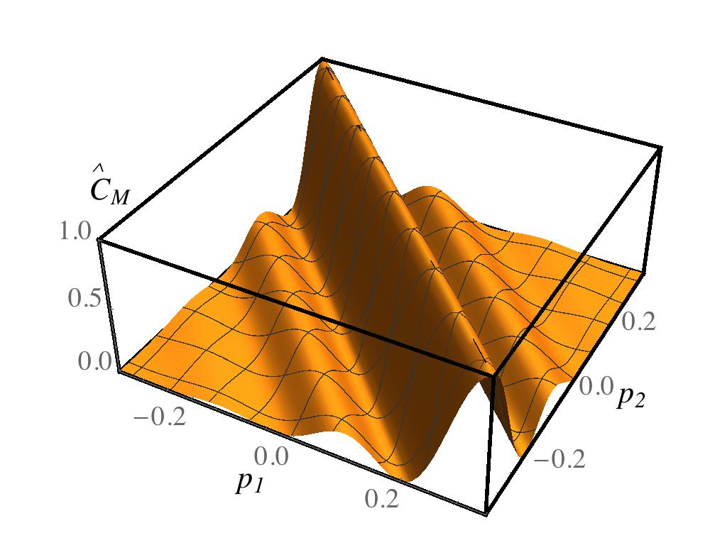
Figure 1: (Color Online) The in-trap momentum correlation function ${\cal C}_{M}(p_{1},p_{2})=\langle n_{p_{1}\uparrow}n_{p_{2}\downarrow}\rangle-\langle n_{p_{1}\uparrow}\rangle\langle n_{p_{2}\downarrow}\rangle$ of a balanced 1D trapped fermion gas with attractive interactions, normalized to its value at $p_{1}=p_{2}=0$ (which we call $\hat{{\cal C}}_{M}(p_{1},p_{2})$). This observable, which can be experimentally accessed by a measurement of noise correlations after free expansion of the gas Altman04 , shows a rapid dependence on the sum of the momenta $p_{1}+p_{2}$ (while being almost independent of $p_{1}-p_{2}$), providing a probe of fermionic pairing correlations.

However, a central outstanding question concerns how to directly probe pairing correlations in this system. To address this, we have studied trapped attractively-interacting Fermi gases in 1D using a variational wavefunction that accounts for the remaining trapping potential along the $z$-direction without using the LDA. Our variational wavefunction is of the BCS form, but in which the pairing is among harmonic oscillator states. An additional variational parameter of our wavefunction, beyond the usual BCS coherence factors, is the effective oscillator length of the single-particle states in our basis, which is allowed to be distinct from the actual oscillator length associated with the trapping potential. As discussed below, including this parameter is necessary for the wavefunction to have a physically sensible density profile, and we find a density profile that agrees reasonably well with Bethe Ansatz combined with LDA.

The purpose of this paper is to study pairing and interaction effects in quasi-1D trapped fermionic atomic gases. We find that a striking probe of pairing correlations is the in-trap momentum correlation function ${\cal C}_{M}(p_{1},p_{2})=\langle n_{p_{1}\uparrow}n_{p_{2}\downarrow}\rangle-\langle n_{p_{1}\uparrow}\rangle\langle n_{p_{2}\downarrow}\rangle$ with $p_{1}$ and $p_{2}$ momenta along the $z$-direction and $n_{p\sigma}$ the occupation of the state with momentum $p$ and spin $\sigma$. This quantity can be determined experimentally by measuring real space atom density correlations after free expansion of the gas, as shown theoretically Altman04 and implemented experimentally Greiner05 in the 3D case. In the present 1D case, the free expansion would be along the tube axis after lowering the confining potential along the $z$-direction.

Other recent theoretical work has analyzed expansion of 1D gases, focusing primarily on the imbalanced case Lu ; Bolech12 . Since our interest is understanding pairing correlations, here we study the balanced gas, using a novel oscillator-basis approach. A similar method can apply to imbalanced gases (relevant for the FFLO state), which we will present in a future work DGpaper . In Fig. 1 we plot our results for the normalized quantity $\hat{{\cal C}}_{\rm M}(p_{1},p_{2})\equiv{\cal C}_{M}(p_{1},p_{2})/{\cal C}_{M}(0,0)$ showing a strong dependence on $p_{1}$ and $p_{2}$, that we can connect to the nature of the underlying pairing correlations as discussed below.

This paper is organized as follows. In Sec. II we introduce the system Hamiltonian, describe our pairing wavefunction in the oscillator basis, and explain why we must allow the oscillator length associated with our single-particle states to differ from the trap oscillator length. In Sec. III we compute the variational ground-state energy and provide an analytic result for the effective interaction function appearing in this energy. In Sec. IV, we present the equations that come from minimizing the variational ground-state energy. In Sec. V, we describe our numerical solutions to these variational equations which yield our predictions for the local density and local pairing potential. In Sec. VI, we describe how we obtain the momentum correlation function for a trapped 1D fermion gas and obtain an approximate analytic formula for this quantity. In Sec. VII, we analyze our system using the Bethe ansatz along with the local density approximation, with the comparison to our variational method given in Fig. 3. Finally, we conclude in Sec. VIII.

II Model Hamiltonian and variational wavefunction

Our starting point is a Hamiltonian for an attractively interacting fermion gas confined to a harmonic trap $V({\bf r})=\frac{1}{2}m\big{[}\omega_{\perp}^{2}\rho^{2}+\omega_{z}^{2}z^{2}\big{]}$, with $\omega_{\perp}\gg\omega_{z}$, such that, at sufficiently low fermion density, we can restrict attention to the lowest oscillator level associated with $\omega_{\perp}$. The resulting quasi one-dimensional Hamiltonian, with $\Psi_{\sigma}(z)$ the field operator for spin-$\sigma$, is:

$${\cal H}=\int_{-\infty}^{\infty}dz\,\Big{(}\sum_{\sigma=\uparrow,\downarrow}\Psi_{\sigma}^{\dagger}(z)\Big{[}\frac{p_{z}^{2}}{2m}+V(z)\Big{]}\Psi_{\sigma}(z)$$

$$\qquad\qquad+\lambda\Psi_{\uparrow}^{\dagger}(z)\Psi_{\downarrow}^{\dagger}(z)\Psi_{\downarrow}^{\phantom{\dagger}}(z)\Psi_{\uparrow}^{\phantom{\dagger}}(z)\Big{)},$$ (1)

where $V(z)=\frac{1}{2}m\omega_{z}^{2}z^{2}$ is the trap along the $z$-direction, and the coupling parameter is $\lambda=-2\hbar^{2}/ma_{1D}$ with $a_{1D}$ the one-dimensional scattering length Olshanii98 . We proceed by expressing $\Psi_{\sigma}(z)$ in terms of harmonic oscillator eigenfunctions $\psi_{n}(z)$ (with $n=0,1,\cdots$ the oscillator level index) via:

$$\Psi_{\sigma}(z) = \sum_{n}\psi_{n}(z)a_{n\sigma},$$ (2)

$$\psi_{n}(z) = \frac{1}{\sqrt{2^{n}n!a_{z}}}\frac{1}{\pi^{1/4}}{\rm e}^{-z^{2}/2a_{z}^{2}}H_{n}(z/a_{z}),$$ (3)

with $H_{n}(z)$ the Hermite polynomial and

$$a_{z}=\sqrt{\frac{\hbar}{m\omega_{z}}},$$ (4)

the the oscillator length. The operator $a_{n\sigma}$ annihilates a fermion with spin $\sigma$ in the $n$th harmonic oscillator level with single-particle energy $\epsilon_{n}=\hbar\omega_{z}(n+\frac{1}{2})$. The system Hamiltonian in this basis is, defining $\hat{{\cal H}}={\cal H}/\hbar\omega_{z}$,

$$\hat{{\cal H}}=\sum_{n,\sigma}\hat{\epsilon}_{n}a_{n_{\sigma}}^{\dagger}a_{n_{\sigma}}^{\phantom{\dagger}}+\hat{\lambda}\sum_{n_{i}}\lambda_{\{n_{i}\}}a_{n_{1}\uparrow}^{\dagger}a_{n_{2}\downarrow}^{\dagger}a_{n_{3}\downarrow}^{\phantom{\dagger}}a_{n_{4}\uparrow}^{\phantom{\dagger}},$$ (5)

where the normalized single-particle energy is $\hat{\epsilon}_{n}=\epsilon_{n}/\hbar\omega_{z}$. Here, $\lambda_{\{n_{i}\}}$ is shorthand for

$$\lambda_{n_{1},n_{2},n_{3},n_{4}}\equiv\int_{-\infty}^{\infty}dz\,\psi_{n_{1}}(z)\psi_{n_{2}}(z)\psi_{n_{3}}(z)\psi_{n_{4}}(z),$$ (6)

characterizing interactions among the oscillator states, and we have have introduced

$$\hat{\lambda}=\frac{\lambda}{\hbar\omega_{z}a_{z}}=-2\frac{a_{z}}{a_{1D}},$$ (7)

the dimensionless coupling parameter.

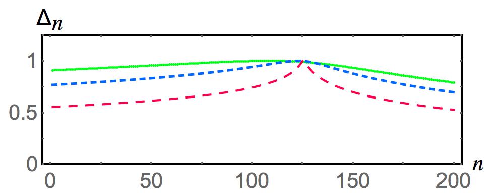
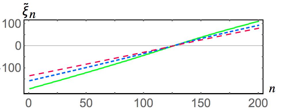
Figure 2: (Color Online) The top panel shows the pairing amplitude for harmonic oscillator level $n$ (normalized to its peak value) and the bottom panel shows the renormalized dispersion $\tilde{\xi}_{n}$ for $\hat{\lambda}=-4.8$ (red, long dashing), $\hat{\lambda}=-13.6$ (blue, short dashing) and $\hat{\lambda}=-22.8$ (green solid) with the total particle number fixed at $N=250$.

In the absence of interactions, the ground state of ${\cal H}$ is simply a Fermi gas in the oscillator basis, with harmonic oscillator levels $n\leq n_{F}$ occupied and $n>n_{F}$ empty. A physically sensible wavefunction that has this limiting case, but which also includes the possibility of pairing correlations among single-particle states, is the following BCS-type variational wavefunction:

$$|\Psi\rangle=\prod_{n}(u_{n}+v_{n}a_{n\uparrow}^{\dagger}a_{n\downarrow}^{\dagger})|0\rangle,$$ (8)

where the coherence factors $u_{n}$ and $v_{n}$ satisfy the constraint $|u_{n}|^{2}+|v_{n}|^{2}=1$. A trapped quasi 1D Fermi gas is not expected to exhibit long-range pairing order. Thus, Eq. (8) should break down on long length scales due to the absence of long-range phase coherence. However, this wavefunction can capture local pairing correlations and their impact on observables like the local density and density-density correlations in a trapped gas. An important task, that we leave for future work, is the investigation of how fluctuations around our variational solution will modify our predictions. For now, our goal is to understand the experimental predictions of Eq. (8).

Before proceeding, however, we note that a crucial drawback of our ansatz, Eq. (8), is that it yields a density profile corresponding to an atom cloud that increases in size along the axial direction in response to increasing attraction. To see the reason for this physically incorrect behavior, consider the noninteracting ($\hat{\lambda}\to 0$) exact ground state, which is a Fermi gas with oscillator states filled up to the Fermi level $n_{\rm F}$. Since the spatial extent of the harmonic oscillator wavefunction at level $n$ is $\simeq a_{z}\sqrt{n}$, we can estimate the cloud size to be approximately proportional to $\sqrt{n_{\rm F}}$ (fixed by the largest filled level). If we now turn on attractive interactions, the Pauli principle means that levels with $n<n_{\rm F}$ cannot increase their occupation, and that oscillator levels with $n>n_{\rm F}$, which have a larger spatial extent, will have a finite amplitude to become occupied. The occupation of such higher levels of course does not imply a spatially larger cloud, since the local axial density operator, expressed in the oscillator basis,

$$\hat{n}(z)=\sum_{n,m,\sigma}\psi^{*}_{n}(z)\psi_{m}(z)a_{n\sigma}^{\dagger}a_{m\sigma}^{\phantom{\dagger}},$$ (9)

has terms that are off-diagonal in the oscillator level. In the true ground state, these off-diagonal terms can lead to cancellations among the terms in Eq. (9), describing a 1D atomic gas that shrinks with increasing attractive interactions.

However, the approximate BCS wavefunction Eq. (8) projects out such off-diagonal terms, yielding the expectation value $n(z)=\langle\Psi|\hat{n}|\Psi\rangle$ given by:

$$n(z)=2\sum_{m=0}^{\infty}\,|\psi_{n}(z)|^{2}|v_{n}|^{2},$$ (10)

which will clearly exhibit a increased cloud size with increasing attractive interactions as higher oscillator levels become occupied, since all terms in the sum are positive.

Remedying this physically incorrect behavior of our variational wavefunction is crucial, since the axial density is a primary observable in cold atom experiments. However, we aim to do this in a way that preserves the simplicity of our BCS variational wavefunction. To accomplish this, we introduce an additional variational parameter, which is the oscillator length associated with our wavefunctions, by replacing $a_{z}\to a$ in Eq. (3) and considering $a$ to be a variational parameter to be minimized. Thus, while the noninteracting fermion gas occupies oscillator states with an oscillator length that is related to the trap potential via Eq. (4), in the interacting case the optimal (lowest energy) BCS-type state may involve oscillator states with $a<a_{z}$ that is smaller, allowing the cloud to shrink in spatial extent. We therefore introduce the parameter

$$\eta=\frac{a_{z}^{2}}{a^{2}},$$ (11)

where $a_{z}$ remains the true oscillator length. Note that we can also write $\eta=\omega/\omega_{z}$ with $\omega$ the frequency of a ficticious trap for which $a$ is the oscillator length. Then, it is convenient to split the trap potential into two pieces, via $V(z)=\frac{1}{2}m\omega^{2}z^{2}+\frac{1}{2}m(\omega_{z}^{2}-\omega^{2})z^{2}$, where the first term yields a contribution to ${\cal H}$ that is identical to Eq. (5) but with $\omega_{z}\to\omega$ and the second term yields a correction that we will evaluate using the properties of the oscillator wavefunctions. We find, upon repeating the preceding analysis for the case of $\eta\neq 1$, the effective Hamiltonian

$$\hat{{\cal H}}=\eta\sum_{n,\sigma}\hat{\epsilon}_{n}a_{n_{\sigma}}^{\dagger}a_{n_{\sigma}}^{\phantom{\dagger}}+\sqrt{\eta}\hat{\lambda}\sum_{n_{i}}\lambda_{\{n_{i}\}}a_{n_{1}\uparrow}^{\dagger}a_{n_{2}\downarrow}^{\dagger}a_{n_{3}\downarrow}^{\phantom{\dagger}}a_{n_{4}\uparrow}^{\phantom{\dagger}}$$

$$+\frac{1}{2}\Big{(}\frac{1}{\eta}-\eta\big{)}\int_{-\infty}^{\infty}dz\,z^{2}\sum_{n_{1},n_{2},\sigma}\hat{\psi}_{n_{1}}^{*}(z)\hat{\psi}_{n_{2}}(z)a_{n_{1}\sigma}^{\dagger}a_{n_{2}\sigma}^{\phantom{\dagger}},$$ (12)

with the second line coming from the abovementioned correction. Here, $\hat{\psi}_{n}(z)$ is a dimensionless Hermite function (Eq. (3) but with $a_{z}\to 1$) and we have once again normalized to $\hbar\omega_{z}$ (as in Eq. (5)).

To summarize this section, Eq. (12) is an expression of our system Hamiltonian in terms of creation and annihilation operators, $a_{n\sigma}$ and $a_{n_{\sigma}}^{\dagger}$, that correspond to harmonic oscillator states with oscillator length $a$ that is different from the physical oscillator length of our system. Here and below $a$ generally appears only via the parameter $\eta$ Eq. (11), and we typically normalize all length scales to $a_{z}$ and all energy scales by $\hbar\omega_{z}$ (for example in figures). Next we proceed by assuming that these oscillator states undergo pairing correlations described by Eq. (8) and determine the optimal coherence factors and value of $a$.

III Variational Energy

Upon taking the expectation value of the Hamiltonian using the wavefunction Eq. (8), in the second line of Eq. (12) the only nonzero contribution comes from $n_{1}=n_{2}$, allowing the $z$ integral to be easily evaluated. We then find that the normalized grand free energy $E_{G}=\langle\hat{{\cal H}}-\hat{\mu}\hat{N}\rangle$ (with $\hat{N}$ the number operator, and $\hat{\mu}=\mu/\hbar\omega_{z}$ the normalized chemical potential) is:

$$E_{G}=2\sum_{n}\xi_{n}|v_{n}|^{2}+\sqrt{\eta}\hat{\lambda}\sum_{n,m}\lambda_{n,m}\big{(}u_{n}^{*}v_{n}^{\phantom{*}}v_{m}^{*}u_{m}^{\phantom{*}}+|v_{n}|^{2}|v_{m}|^{2}\big{)},$$ (13)

where we defined $\xi_{n}=\frac{1}{2}\big{(}\eta+\eta^{-1}\big{)}n+\frac{1}{2}-\hat{\mu}$. Here and below we focus on zero temperature. In the interaction part of Eq. (13), the first term corresponds to pairing correlations and the second term corresponds to Hartree-Fock correlations. Here, $\lambda_{m,n}\equiv\lambda_{n,n,m,m}$ is the effective interaction resulting from our variational ansatz, explicitly given by:

$$\lambda_{m,n}=\frac{1}{2^{m+n}}\frac{1}{\pi n!m!}\int_{-\infty}^{\infty}dz\,{\rm e}^{-2z^{2}}H_{n}^{2}(z)H_{m}^{2}(z).$$ (14)

Integrals of this form have been of interest to the mathematical physics community Wang , and have also recently appeared in other cold-atom contexts Rey . Although it can be evaluated numerically, this becomes difficult for large $m$ and $n$. We next present our analytic result for Eq. (14), that greatly sped-up our calculations. To do this we use an identity for the square of a Hermite polynomial, $H_{n}^{2}(z)=2^{n}(n!)^{2}\sum_{s=0}^{n}\frac{H_{2s}(z)}{2^{s}(s!)^{2}(n-s)!}$, for the two factors $H_{n}^{2}(z)$ and $H_{m}^{2}(z)$ in Eq. (14). This leads to a $z$-integral involving a product of two Hermite polynomials multiplying the Gaussian factor ${\rm e}^{-2z^{2}}$ that appears in Gradshteyn and Ryzhik Gradshteynintegral ; Gradshteyn . Then, evaluating the remaining summations, we obtain:

$$\lambda_{m,n}=\frac{(-1)^{m}}{\sqrt{2}m!}\frac{{}_{3}F_{2}(\frac{1}{2},\frac{1}{2},-n;1,\frac{1}{2}-m;1\big{)}}{\Gamma[\frac{1}{2}-m]},$$ (15)

with ${}_{3}F_{2}$ the generalized hypergeometric function. Although it is not obvious from Eq. (15), $\lambda_{m,n}$ is indeed symmetric under interchange of its indices.

IV Variational equations

We now proceed with minimizing Eq. (13) with respect to our variational parameters. To minimize with respect to the $u_{n}$ and $v_{n}$, we must enforce the constraint $|u_{n}|^{2}+|v_{n}|^{2}=1$ with a Lagrange multiplier $E_{n}$. The resulting Euler-Lagrange equations take the form of a Bogoliubov-de Gennes (BdG) eigenvalue problem

$$\begin{pmatrix}\xi_{n}+U_{n}&\Delta_{n}\\ \Delta_{n}^{*}&-\xi_{n}-U_{n}\end{pmatrix}\begin{pmatrix}u_{n}\\ v_{n}\end{pmatrix}=E_{n}\begin{pmatrix}u_{n}\\ v_{n}\end{pmatrix},$$ (16)

where we defined the strength of pairing correlations $\Delta_{n}\equiv-\hat{\lambda}\sqrt{\eta}\sum_{m}\lambda_{n,m}v_{m}^{*}u_{m}$ and the Hartree-Fock energy shift $U_{n}\equiv\hat{\lambda}\sqrt{\eta}\sum_{m}\lambda_{n,m}|v_{m}|^{2}$. Defining the renormalized single-particle energy $\tilde{\xi}_{n}=\xi_{n}+U_{n}$, we obtain the BdG solution $u_{n}=\frac{1}{\sqrt{2}}\sqrt{1+\frac{\tilde{\xi}_{n}}{E_{n}}}$ and $v_{n}=\frac{1}{\sqrt{2}}\sqrt{1-\frac{\tilde{\xi}_{n}}{E_{n}}}$, with $E_{n}=\sqrt{\tilde{\xi}_{n}^{2}+\Delta_{n}^{2}}$. Inserting these solutions into the definitions of $\Delta_{n}$ and $U_{n}$ then leads to the self-consistency conditions

$$\Delta_{n} = -\hat{\lambda}\sqrt{\eta}\sum_{m=0}^{\infty}\lambda_{n,m}\frac{\Delta_{m}}{2E_{m}},$$ (17a)

$$U_{n} = \hat{\lambda}\sqrt{\eta}\sum_{m=0}^{\infty}\lambda_{n,m}\frac{1}{2}\big{(}1-\frac{\tilde{\xi}_{m}}{E_{m}}\big{)}.$$ (17b)

A third variational equation comes from minimizing $E_{G}$ with respect to the parameter $\eta$ that determines the optimal oscillator length characterizing our basis set. We find, differentiating $E_{G}$ with respect to $\eta$,

$$0=\sum_{n}|v_{n}|^{2}\big{(}n+\frac{1}{2}\big{)}\big{(}1-\frac{1}{\eta^{2}}\big{)}$$ (18)

$$\qquad+\frac{1}{2\sqrt{\eta}}\hat{\lambda}\sum_{n}\lambda_{n,m}\big{(}u_{n}^{*}v_{n}v_{m}u_{m}+|v_{n}|^{2}|v_{m}|^{2}\big{)}.$$

We see that the parameter $\eta$ multiplies $\hat{\lambda}$ in Eqs. (17) determining the $u_{n}$ and $v_{n}$. Since we expect $\eta>1$ in equilibrium, this implies an effectively larger coupling in equilibrium, consistent with the picture of the central density increasing due to the presence of attractive interactions.

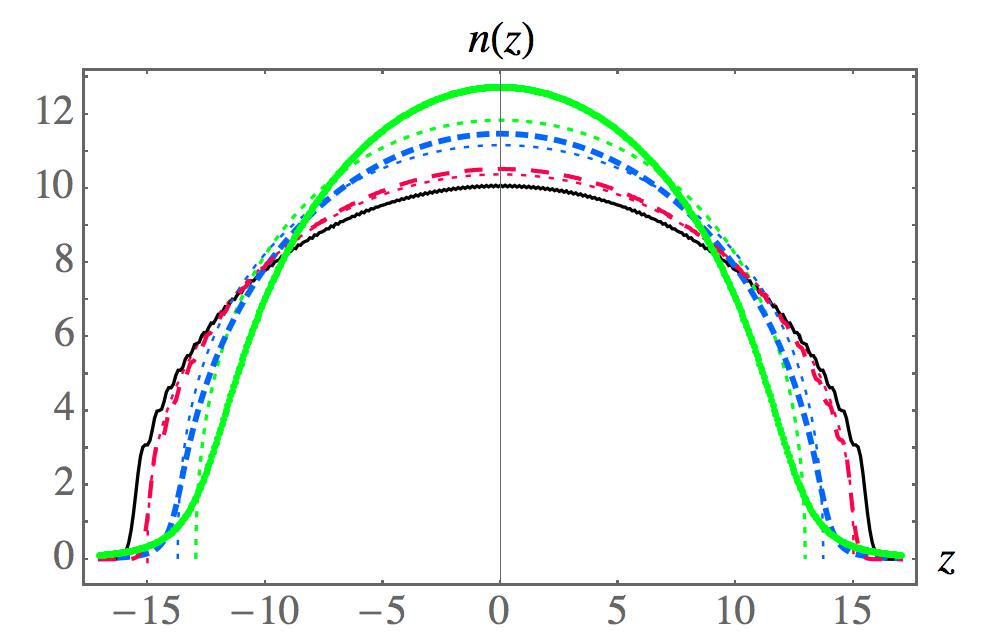
Figure 3: (Color Online) The thick lines show the axial density $n(z)$ (in dimensionless units) resulting from our variational approach, as a function of position (normalized to the inverse oscillator length) for the same parameters as Fig. 2 (total particle number $N=250$ with $\hat{\lambda}=-4.8$ being red, long dashing; $\hat{\lambda}=-13.6$ being blue, short dashing, and $\hat{\lambda}=-22.8$ solid green). Each such curve has a corresponding nearby dotted curve (with the same color scheme that, for $z=0$, is just below the variational result) that is the result of Bethe ansatz along with the local density approximation for the same values of the dimensionless coupling constant and particle number. The solid thin black curve that is the lowest at $z=0$ is the noninteracting case.

V Results

The simultaneous numerical solution of Eqs. (17) and Eq. (18), yielding the variational parameters describing our system ($\Delta_{n}$, $U_{n}$, and $\eta$), was done numerically, although an approximate analytic solution can be found in the extreme weak-coupling limit $\hat{\lambda}\to 0$ as described below. Our numerical calculations were conducted for three values of the dimensionless coupling ($\hat{\lambda}=-4.8$, $\hat{\lambda}=-13.6$ and $\hat{\lambda}=-22.8$) with the particle number held at $N=250$ (requiring an adjustment of the system chemical potential). For comparison, the coupling in Ref. LiaoRittner was $\hat{\lambda}\simeq-52$.

For our numerical procedure we truncated the sums in Eqs. (17) at an upper cutoff $n_{\rm max}=350$ (outside the plotted range of Fig. 2). An estimate of the error involved in this truncation comes from the value of $|v_{n_{\rm max}}|^{2}=(2.9\times 10^{-7},1.8\times 10^{-4},2.6\times 10^{-3})$ for $\hat{\lambda}=-4.8$, $\hat{\lambda}=-13.6$ and $\hat{\lambda}=-22.8$, respectively, which we argue to be negligible except perhaps in the $\hat{\lambda}=-22.8$ case. For this coupling, we fit $|v_{n}|^{2}$ to a power law for $n$ close to $n_{\rm max}$, and obtained a better error estimate by extrapolating this beyond $n_{\rm max}$ and determining the expected number of fermions in levels above $n_{\rm max}$, which we find to be $\Delta N\simeq 2\int_{n_{\rm max}}^{\infty}dn\,|v_{n}|^{2}\simeq 0.5$, much smaller than the total particle number.

In Fig. 2 (top panel), we plot our numerical results for the pairing amplitude ($\Delta_{n}$), normalized to its maximum value $\Delta_{\rm max}$. The maximum pairing amplitudes were $\Delta_{\rm max}=0.71$, $\Delta_{\rm max}=15.0$ and $\Delta_{\rm max}=57.1$, for the coupling values $\hat{\lambda}=-4.8$, $\hat{\lambda}=-13.6$ and $\hat{\lambda}=-22.8$ respectively, with the corresponding equilibrium $\eta$ values being $\eta=1.09$, $\eta=1.31$ and $\eta=1.67$, with the latter describing a cold-atom cloud that shrinks in the axial direction, effectively occupying oscillator states with $a<a_{z}$.

The weakest coupling $\hat{\lambda}=-4.8$ plot (red dashed) shows that $\Delta_{n}$ is narrowly peaked near the Fermi level $n_{F}\approx 125$ (defined by when $\tilde{\xi}_{n}$ comes closest to zero), consistent with the general expectation that pairing is strongest near $n_{F}$. We can approximately derive this behavior analytically in the weak coupling (small $|\hat{\lambda}|$) limit by noting that, in this limit, the sum on the right side of Eq. (17a) is dominated by terms near $n_{F}$. If we approximate $\eta\approx 1$, take the dispersion to have the form $\tilde{\xi}_{n}=n-n_{F}$, and keep only the term $n=n_{F}$ in the sum, we obtain $\Delta_{n}=\frac{1}{2}|\hat{\lambda}|\lambda_{n,n_{F}}$, so that the shape of $\Delta_{n}$ approximately reflects the shape of the coupling function Eq. (15). While this result qualitatively captures the $n$ dependence of the pairing amplitude, it is only quantitatively valid for $|\hat{\lambda}|\ll 1$ and does not approximately describe our results for any of the displayed coupling values. With increasing attraction, $\Delta_{n}$ broadens considerably as more levels participate in pairing, as seen by the $\hat{\lambda}=-13.6$ (blue, short-dashing) and $\hat{\lambda}=-22.8$ (green, solid) curves of Fig. 2 (top panel).

The bottom panel of Fig. 2 shows the renormalized dispersion $\tilde{\xi}_{n}$ for the same three coupling values, showing that this quantity is approximately linear near $n_{F}$ for all coupling values but with a renormalized slope, with $\tilde{\xi}_{n}=\alpha(n-n_{F})$ where $\alpha$ increases with increasing coupling strength.

We now turn to the question of how interaction effects would be revealed in experiments. A natural observable accessible in cold atom experiments is the axial density $n(z)$ as a function of position, given by Eq. (10) above and plotted in Fig. 3 for the same three coupling values (thick, with the same color and dashing scheme as in Fig. 2). The thin dotted curves that are adjacent to our variational wavefunction results (with the same color scheme) are the results of combining the Bethe ansatz with the local density approximation (for the same parameters and particle number, with details provided in Sec. VII), and the lowest solid curve is the noninteracting case.

This figure shows that our variational method agrees quantitatively with the Bethe ansatz plus LDA for the weakest coupling $\hat{\lambda}=-4.8$ case. Since both curves are clearly distinct from the noninteracting case, this is not merely due to the fact that they are all in the noninteracting limit, although both the variational method and the Bethe ansatz plus LDA methods agree with the noninteracting curve for smaller coupling (for example, $\hat{\lambda}\simeq-0.1$).

Increasing the magntitude of the coupling strength causes the cloud to shrink in size (as expected), although the discrepancy between our variational results and the Bethe ansatz plus LDA also increases. We note that, a priori, it is not clear which theoretical method is more accurate since both are approximate, although we expect the Bethe ansatz plus LDA to be more accurate in the limit of a more uniform local density (which, here, occurs for smaller $|\hat{\lambda}|$)

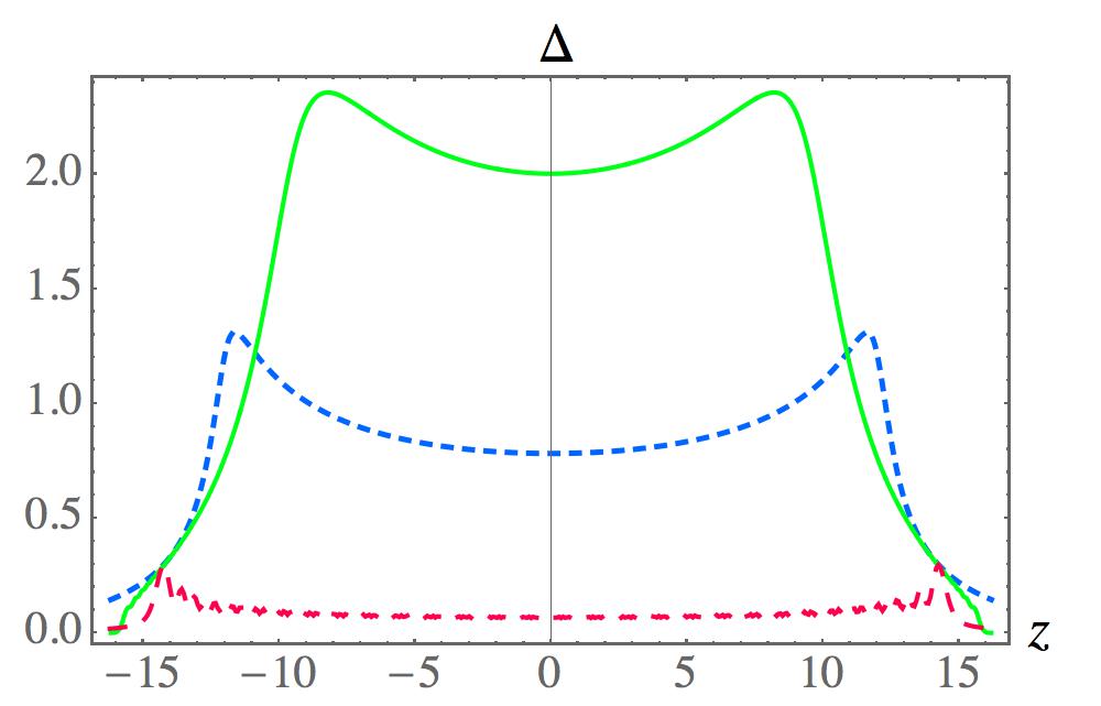
Figure 4: (Color Online) The local pairing amplitude $\Delta(z)$ (normalized to $\hbar\omega_{z}$), as a function of position (normalized to the oscillator length) for the same parameters as Fig. 2, showing a significant increase in the local pairing with increasing attraction.

We now turn to the local pairing amplitude $\Delta(z)\equiv\langle\Psi_{\uparrow}(z)\Psi_{\downarrow}(z)\rangle$, given, within the present variational approach, by:

$$\Delta(z)=\sum_{n=0}^{\infty}\big{(}\psi_{n}(z)\big{)}^{2}v_{n}u_{n},$$ (19)

which we plot in Fig. 4. Strictly speaking, $\Delta(z)$ is not directly observable since it is off-diagonal in fermion field operators. However, it does provide information about the increasing strength of pairing correlations with increasing magnitude of $\hat{\lambda}$.

One way to estimate the validity of our approach is to calculate the local BCS coherence length, given by $\xi=\frac{\hbar v_{\rm F}}{\pi\Delta}$ for a uniform system. If $\xi$ is much larger than the typical interparticle spacing, then one expects fluctuations around our solution to be relatively small. To determine this, we use the uniform-case result for the Fermi wavevector, $k_{\rm F}=\pi n/2$ (with $n$ the 1D atom density), in terms of which $v_{\rm F}=\hbar k_{\rm F}/m$. Combining these gives

$$\xi n=\hbar^{2}n^{2}/(2m\Delta),$$ (20)

for the coherence length normalized to the interparticle spacing $n^{-1}$. The quantities on the right side, $n$ and $\Delta$, are plotted in Figs. 3 and 4, but in dimensionless forms (normalized to $a_{z}^{-1}$ and $\hbar\omega_{z}$, respectively). Converting the right side of this formula to dimensionless form yields $\hbar^{2}n^{2}/(2m\Delta)\to n^{2}/(2\Delta)$ so that the normalized coherence length is simply the square of a curve in Fig. 3 divided by a curve Fig. 4. Thus, we find $\xi n\gtrsim 10$ for all coupling values, indicating that the coherence length is large compared to the interparticle spacing. This, along with the approximate agreement with Bethe ansatz along with the LDA, gives further confidence in the validity of our approach.

In the next section, we consider an observable, the momentum correlation function, which also probes the strength of pairing correlations in a balanced 1D fermion gas.

VI Momentum correlation function

To find a sensitive probe of pairing we turn to the momentum correlation function ${\cal C}_{M}(p_{1},p_{2})=\langle n_{p_{1}\uparrow}n_{p_{2}\downarrow}\rangle-\langle n_{p_{1}\uparrow}\rangle\langle n_{p_{2}\downarrow}\rangle$, with $n_{p\sigma}=c_{p\sigma}^{\dagger}c_{p\sigma}$ the momentum occupation operator. As shown by Altman et al, ${\cal C}_{M}(p_{1},p_{2})$ is probed by the real-space noise correlation function ${\cal C}(z_{1},z_{2})=\langle n_{\uparrow}(z_{1})n_{\downarrow}(z_{2})\rangle-\langle n_{\uparrow}(z_{1})\rangle\langle n_{\downarrow}(z_{2})\rangle$, of the freely-expanded gas. Thus, assuming the absence of interaction effects during expansion for time $t$, ${\cal C}(z_{1},z_{2})$ is directly proportional to ${\cal C}_{M}(p_{1},p_{2})$, with $p_{1}=mz_{1}/t$ and $p_{2}=mz_{2}/t$. Using our variational wavefunction, we find ${\cal C}_{M}(p_{1},p_{2})\propto|S(p_{1},p_{2})|^{2}$ with the sum

$$S(p_{1},p_{2})=\sum_{n=0}^{\infty}\chi^{\phantom{*}}_{n}\big{(}p_{1}\big{)}\chi^{\phantom{*}}_{n}\big{(}p_{2}\big{)}u_{n}^{*}v_{n}^{\phantom{*}},$$ (21)

where

$$\chi_{n}(p) = \int_{-\infty}^{\infty}dz\,{\rm e}^{-ipz}\psi_{n}(z),$$ (22)

$$= (-i)^{n}\frac{\pi^{1/4}\sqrt{a}}{\sqrt{2^{n-1}n!}}{\rm e}^{-a^{2}p^{2}/2}H_{n}(pa),$$ (23)

are the Fourier-transforms of the harmonic oscillator wavefunctions (that we emphasize contain $a$, the oscillator-length variational parameter).

Our results for the momentum correlation function look, qualitatively, like Fig. 1 for all coupling values, where we plotted the normalized function $\hat{{\cal C}}_{M}(p_{1},p_{2})\equiv{\cal C}_{M}(p_{1},p_{2})/{\cal C}_{M}(0,0)$. Thus, $\hat{{\cal C}}_{M}(p_{1},p_{2})$ is sharply peaked around $p_{1}+p_{2}=0$, and is, approximately, only a function of the sum $|p_{1}+p_{2}|$ of the momenta. To understand the rapid variation as a function of $|p_{1}+p_{2}|$, in Fig. 5, we plot the equal momenta correlator $\hat{{\cal C}}_{M}(p,p)$ for all three coupling values (using the same color and dashing scheme as above), along with a fourth curve (black dots) that is an approximate analytic evaluation of $\hat{{\cal C}}_{M}(p,p)$ for the case of $\hat{\lambda}=-22.8$ that we now describe.

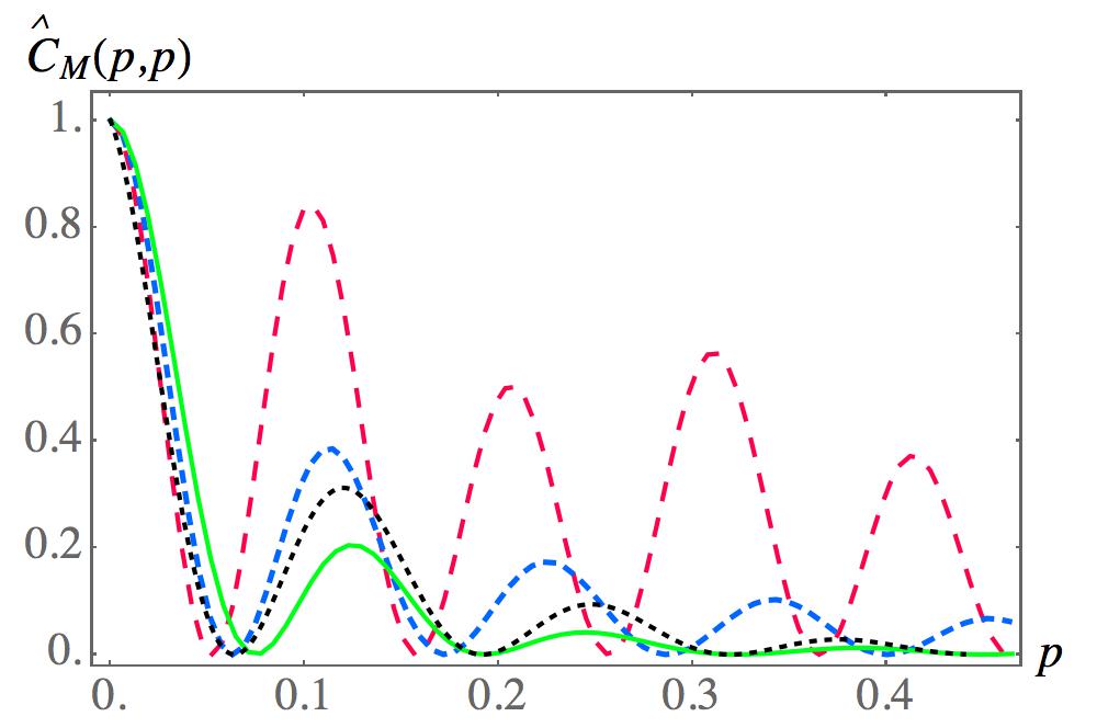
Figure 5: (Color Online) The normalized momentum correlation function, $\hat{{\cal C}}_{M}(p_{1},p_{2})$ in the limit $p_{1}=p_{2}=p$ (normalized to unity at $p\to 0$), for a trapped 1D fermionic superfluid, for the same three coupling values as Figs. 2 and 3. A fourth curve, black dots, depicts the approximate theoretical formula Eq. (25) for the case of $\hat{\lambda}=-22.8$ which should be compared to the green solid curve, our numerical result for this case. Here we chose units for the momentum axis such that $a_{z}=1$.

Our approximate form for the correlator follows by noting that the summand of Eq. (21), $u_{n}^{*}v_{n}^{\phantom{*}}=\frac{\Delta_{n}}{2E_{n}}$, is narrowly peaked for $n$ close to the Fermi level, with an approximate Lorentzian shape for $n\to n_{F}$ given by $u_{n}^{*}v_{n}^{\phantom{*}}\simeq\frac{1}{2}\frac{1}{1+(n-n_{F})^{2}/w^{2}},$ where $w=\sqrt{2}\Delta_{n_{F}}/\alpha$ approximately represents the number of harmonic oscillator levels that are paired. Here, we recall that $\alpha$ is the slope of the effective dispersion near the Fermi level, with $\tilde{\xi}_{n}=\alpha(n-n_{F})$. From the $\hat{\lambda}=-22.8$ results we find $\alpha\simeq 1.66$ and $\Delta_{n_{F}}\simeq 56.4$, yielding $w\simeq 48.0$.

Expressing the Lorentzian in an integral form, $[1+(n-n_{F})^{2}/w^{2}]^{-1}=w\int_{0}^{\lambda}d\lambda\,{\rm e}^{-\lambda w}\cos\lambda(n-n_{F})$, we can evaluate the sum to get (with being the real part):

$$S(p_{1},p_{2})=w\int_{0}^{\infty}d\lambda\,{\rm e}^{-\lambda w}\,\big{(}{\rm e}^{i\lambda n_{F}}K\big{[}{\rm e}^{-i\lambda}\big{]}\big{)},$$ (24)

where $K[x]\equiv\frac{\sqrt{\pi}}{\sqrt{1-x^{2}}}\exp\big{[}\frac{(p_{1}^{2}+p_{2}^{2})(1+x^{2})+4p_{1}p_{2}x}{2(x^{2}-1)}\big{]}$. The dominant contribution to this integral comes the regime where $\lambda\to 0$. Expanding $K\big{[}{\rm e}^{-i\lambda}\big{]}$ in this limit yields an integral that can be easily evaluated analytically. Finally taking the limit $w\ll n_{F}$ for simplicity, we find for the normalized correlator:

$$\!\!\!\hat{{\cal C}}_{\rm M}(p_{1},p_{2})=\cos^{2}\big{[}\sqrt{2n_{F}}|p_{1}+p_{2}|a\big{]}{\rm e}^{-\sqrt{2}w|p_{1}+p_{2}|a/\sqrt{n_{F}}},$$ (25)

which we find to be qualitatively accurate, as seen in Fig. 5, connecting the local pairing and Hartree-Fock correlations to this observable.

As shown in Fig. 1, our numerical evaluation of $\hat{{\cal C}}_{\rm M}(p_{1},p_{2})$ yields a result that is nearly independent of the difference in momenta $p_{1}-p_{2}$, a feature that appears in the approximate result Eq. (25). However, we find that the degree to which $\hat{{\cal C}}_{\rm M}(p_{1},p_{2})$ is independent of $p_{1}-p_{2}$ is rather sensitive to the choice of the upper cutoff $n_{\rm max}$ in our numerical summation, and leave further investigation of this to future work.

We also see that, within the approximations leading to Eq. (25), the oscillatory variation of this correlation function as a function of the sum of momenta measures the uppermost occupied oscillator state (Fermi level $n_{F}$), and the exponential decay measures the strength of pairing at the Fermi level (via the parameter $w$). Thus, the momentum correlation function indeed provides a direct probe of pairing correlations in a trapped 1D interacting Fermi gas.

VII Bethe ansatz and LDA

In the present paper, our goal was to pursue a variational wavefunction scheme, based on a BCS type wavefunction in the oscillator basis, to analyze attractively interacting fermions in a one-dimensional trapping potential. In this section, we re-analyze our model Hamiltonian Eq. (1) within a different approximation scheme, namely the Bethe ansatz (exact for an infinite system, or $V(z)=0$) along with the local density approximation to handle the trap. Such a method was used in Ref. LiaoRittner in the imbalanced case and found to exhibit remarkable agreement with experimental results for the density profile.

To implement the Bethe ansatz, we follow the recent review of Guan et al Guan , taking the limit $\rho_{1}(k)=0$ of Eqs.(13) of Ref. Guan (appropriate for the balanced case studied here). Then, the density of pairs at quasimomentum $k$, $\rho(k)$, satisfies the Fredholm equation

$$\rho(k)=\frac{1}{\pi}+\int_{-A}^{A}dk^{\prime}\,K(k-k^{\prime})\rho(k^{\prime}),$$ (26)

with $K(x)=\frac{1}{\pi}\frac{c}{c^{2}+x^{2}}$, where $c$ is proportional to the 1D coupling constant (as defined below) The parameter $A$ is chosen so that the system has the correct total number of particles.

To implement the Bethe ansatz, it is convenient to rescale coordinates in the Hamiltonian Eq. (1) via $z\to a_{z}z$ with $a_{z}$ the oscillator length and define new fields $\Psi_{\sigma}(a_{z}z)=\tilde{\Psi}_{\sigma}(z)/\sqrt{a_{z}}$. This leads to:

$${\cal H}=\int_{-\infty}^{\infty}dz\,\Big{(}\sum_{\sigma}\tilde{\Psi}_{\sigma}^{\dagger}(z)\Big{[}\frac{p_{z}^{2}}{2ma_{z}^{2}}+\frac{1}{2}ma_{z}^{2}\omega_{z}^{2}z^{2}\Big{]}\tilde{\Psi}_{\sigma}(z)$$

$$\qquad\qquad+\frac{\lambda}{a_{z}}\tilde{\Psi}_{\uparrow}^{\dagger}(z)\tilde{\Psi}_{\downarrow}^{\dagger}(z)\tilde{\Psi}_{\downarrow}^{\phantom{\dagger}}(z)\tilde{\Psi}_{\uparrow}^{\phantom{\dagger}}(z)\Big{)},$$ (27)

which we see describes fermions of effective mass $m_{\rm eff}=ma_{z}^{2}$ and effective coupling $\lambda/a_{z}$. Thus, while Guan et al quote the relation $\lambda=\hbar^{2}c/m$ between the coupling constant and the parameter $c$, in the present context we should use this formula with the replacement $\lambda\to\lambda/a_{z}$ and $m\to ma_{z}^{2}$. This leads to:

$$c=-\frac{2a}{a_{1D}},$$ (28)

conveniently equal to our dimensionless parameter $\hat{\lambda}$ defined in Eq. (7).

Once we determine $\rho(k)$, via a numerical solution of Eq. (26) for a chosen value of $A$, the total particle number density $n$ and the dimensionless internal energy density are given by Guan :

$$n = 2\int_{-A}^{A}dk\,\rho(k),$$ (29)

$$\hat{E} = \int_{-A}^{A}dk\,(2k^{2}-c^{2}/2)\rho(k).$$ (30)

Note that, to obtain the system chemical potential, we need the dimensionful energy density $E=\hbar^{2}/(2m_{\rm eff})\hat{E}$, in terms of which $\mu=\frac{\partial E}{\partial n}$. Then, the normalized chemical potential $\hat{\mu}=\mu/\hbar\omega_{z}$ will be given by:

$$\hat{\mu}=\frac{1}{2}\frac{\partial\hat{E}}{\partial n}.$$ (31)

To produce the curves in Fig. 3, then, we obtained $n$ and $\hat{E}$ as a function of the parameter $A$, which can be combined to yield $\hat{\mu}$ via Eq. (31) and hence $n$ as a function of $\hat{\mu}$. Note that the dimensionless density and coordinate comprising the vertical and horizontal axes of Fig. 3 are identical to $n$ and $z$ of this section (due to the abovementioned rescaling). Thus, to implement the LDA, we obtain $n(z)$ from

$$n(z)=n(\hat{\mu}-\frac{1}{2}z^{2}),$$ (32)

with the function on the right being $n(\hat{\mu})$ as described above. The central chemical potential in this formula is chosen to fix the total particle number $N\simeq 250$ for each case.

VIII Concluding remarks

To conclude, although quasi 1D trapped Fermi gases are not expected to exhibit long-range pairing order, short ranged pairing correlations will be induced by the tunable attractive interactions and can be modeled by the simple variational wavefunction Eq. (8). Our theoretical approach, which does not rely on the LDA (although it treats interaction effects approximately), can easily be implemented for experimentally realistic system parameters and, as shown here, leads to specific predictions for how such pairing correlations impact the momentum correlation function. Since our approach agrees with the results of Bethe ansatz plus LDA (at least in the weak coupling limit when the latter becomes more accurate), it provides a simple description of trapped interacting fermionic atomic gases.

We gratefully acknowledge useful discussions with A. Chubukov, R. Fernandes, F. Heidrich-Meisner, R. Hulet, A.M. Rey, and I. Vekhter. This work was supported by the National Science Foundation Grant No. DMR-1151717. This work was supported in part by the National Science Foundation under Grant No. PHYS-1066293 and the hospitality of the Aspen Center for Physics. DES acknowledges support from the German Academic Exchange Service (DAAD) and the hospitality of the Institute for Theoretical Condensed Matter physics at the Karlsruhe Institute of Technology.

References

- (1) I. Bloch, J. Dalibard, and W. Zwerger, Rev. Mod. Phys. 80, 885-964 (2008).
- (2) S. Giorgini, L.P. Pitaevskii, and S. Stringari, Rev. Mod. Phys. 80, 1215 (2008).
- (3) X.-W. Guan, M.T. Batchelor, and C. Lee, Rev. Mod. Phys. 85, 1633 (2013).
- (4) P. Fulde and R.A. Ferrell, Phys. Rev. 135, A550 (1964).
- (5) A.I. Larkin and Yu.N. Ovchinnikov, Zh. Eksp. Teor. Fiz 47, 1136 (1964) [Sov. Phys. JETP 20, 762 (1965)].
- (6) Y. Liao, A.S.C. Rittner, T. Paprotta, W. Li, G.B. Partridge, R.G. Hulet, S.K. Baur, and E.J. Mueller, Nature (London) 467, 567-569 (2010).
- (7) G. Orso, Phys. Rev. Lett. 98, 070402 (2007).
- (8) H. Hu, X.-J. Liu, and P.D. Drummond, Phys. Rev. Lett. 98, 070403 (2007).
- (9) For a review see L. Radzihovsky and D.E. Sheehy, Rep. Prog. Phys. 73, 076501 (2010).
- (10) L. Radzihovsky and A. Vishwanath, Phys. Rev. Lett. 103, 010404 (2009); L. Radzihovsky, Phys. Rev. A 84, 023611 (2011).
- (11) A. E. Feiguin and F. Heidrich-Meisner, Phys. Rev. B 76, 220508 (2007).
- (12) X.-J. Liu, H. Hu, and P. D. Drummond, Phys. Rev. A 76, 043605 (2007).
- (13) G. G. Batrouni, M.H. Huntley, V.G. Rousseau, and R.T. Scalettar, Phys. Rev. Lett. 100, 116405 (2008).
- (14) F. Heidrich-Meisner, A.E. Feiguin, U. Schollwöck, and W. Zwerger, Phys. Rev. A 81, 023629 (2010).
- (15) K. Sun, J.S. Meyer, D.E. Sheehy, and S. Vishveshwara, Phys. Rev. A 83, 033608 (2011).
- (16) K. Sun and C.J. Bolech, Phys. Rev. A 85, 051607 (2012).
- (17) E. Altman, E. Demler, and M.D. Lukin, Phys. Rev. A 70, 013603 (2004).
- (18) M. Greiner, C.A. Regal, J.T. Stewart, D.S. Jin, Phys. Rev. Lett. 94, 110401 (2005).
- (19) H. Lu, L.O. Baksmaty, C.J. Bolech, and H. Pu, Phys. Rev. Lett. 108, 225302 (2012).
- (20) C.J. Bolech, et al, Phys. Rev. Lett. 109, 110602 (2012).
- (21) D.M. Gautreau, S. Kudla, and D.E. Sheehy, in preparation.
- (22) M. Olshanii, Phys. Rev. Lett. 81, 938 (1998).
- (23) W.-M. Wang, Commun. Math. Phys. 277, 459 (2008); W.-M. Wang, preprint http://arxiv.org/abs/0901.3970
- (24) A.M. Rey, A.V. Gorshkov, C.V. Kraus, M.J. Martin, M. Bishof, M.D. Swallows, X. Zhang, C. Benko, J. Ye, N.D. Lemke, and A.D. Ludlow, Annals of Physics. 340, 311 (2014).
-
(25)
The necessary integral is (for and integers) Gradshteyn :
- (26) I.S. Gradshteyn and I.M. Ryzhik, Table of Integrals, Series, and Products.