Model-based clustering using copulas with applications

Abstract

The majority of model-based clustering techniques is based on multivariate Normal models and their variants. In this paper copulas are used for the construction of flexible families of models for clustering applications. The use of copulas in model-based clustering offers two direct advantages over current methods: i) the appropriate choice of copulas provides the ability to obtain a range of exotic shapes for the clusters, and ii) the explicit choice of marginal distributions for the clusters allows the modelling of multivariate data of various modes (either discrete or continuous) in a natural way. This paper introduces and studies the framework of copula-based finite mixture models for clustering applications. Estimation in the general case can be performed using standard EM, and, depending on the mode of the data, more efficient procedures are provided that can fully exploit the copula structure. The closure properties of the mixture models under marginalization are discussed, and for continuous, real-valued data parametric rotations in the sample space are introduced, with a parallel discussion on parameter identifiability depending on the choice of copulas for the components. The exposition of the methodology is accompanied and motivated by the analysis of real and artificial data.
Keywords: mixture models; dependence modelling; parametric rotations; multivariate discrete data; mixed-domain data.

1 Introduction

1.1 Finite Mixture models for real-valued data

The use of finite mixture models in clustering is finding a large number of applications, mainly because it allows standard statistical modelling tools to be used in order to assess and evaluate the clustering. The density or probability mass function of a finite mixture model is defined as

$$h({\bm{x}};{\bm{\theta}},{\bm{\pi}})=\sum_{j=1}^{k}\pi_{j}f_{j}({\bm{x}};{\bm{\theta}}_{j})\quad({\bm{x}}\in\Re^{p})\,,$$ (1)

where ${\bm{\theta}}=({\bm{\theta}}_{1}^{\top},\ldots,{\bm{\theta}}_{k}^{\top})^{\top}\in\Theta_{1}\times\ldots\times\Theta_{k}$, and $\pi_{j}\in(0,1)$ with $\sum_{j=1}^{k}\pi_{j}=1$. Appropriate choices of $f_{j}({\bm{x}};{\bm{\theta}}_{j})$ can result in flexible models of small complexity. Banfield and Raftery (1993) and the book of McLachlan and Peel (2000) provide a detailed treatment of the framework of finite mixture modelling for clustering.

For continuous data, a common choice for the component densities $f_{j}({\bm{x}};{\bm{\theta}}_{j})$ $(j=1,\ldots,k)$ is the density of the multivariate Normal distribution. This is mainly because of the convenience it offers in estimation (closed-form maximization steps in the EM algorithm) and interpretation (easy marginalization for visualising fitted components and the mixture density). The resultant clusters, though, are limited to be elliptical in shape, and as is demonstrated in Hennig (2010), one may need more than one multivariate Normal components, in order to fit a single non-elliptical cluster.

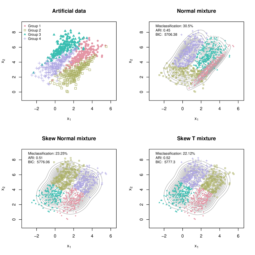
Figure 1: An artificial data set with observations on two continuous variables (top left), a fitted mixture of four 2-dimensional Normal distributions (top right), a fitted mixture of four 2-dimensional skew-Normal distributions (bottom left) and a fitted mixture of four 2-dimensional skew-t distributions (bottom right).

Such restrictions of multivariate Normal finite mixtures have resulted in an expanding literature where other special component distributions are considered. Prominent examples of alternative component densities include multivariate $t$ distributions (see, Andrews and McNicholas, 2011), multivariate skew-Normal and skew-$t$ distribution (see, for example, Frühwirth-Schnatter and Pyne, 2010; Lee and McLachlan, 2014), multivatiate skew student-$t$-Normal distributions (Lin et al., 2014), multivariate Normal inverse Gaussian distributions (Karlis and Santourian, 2009). Other attempts can be found in Forbes and Wraith (2014) for finite mixtures of multivariate scaled Normal distributions and (Morris and McNicholas, 2013) for mixtures of shifted asymmetric Laplace distributions. The results of such studies indicate that the introduction of heavy tails and/or skewness allows the construction of more parsimonious models than multivariate Normal mixtures, which can also bridge the gap between the number of clusters present in the data and the number of components used in the mixture.

Despite the added flexibility that such mixture models offer, all of them force the data to obey very specific marginal properties, and they are not appropriate, for example, in cases where the simultaneous treatment of real-valued observations, strictly positive and observations in $(0,1)$ is needed. In such cases one needs to either ignore the range of the variables and treat them as real-valued or apply appropriate transformations that map the original range of the observations on the real line. Furthermore, even for real-valued variables, as Example 1.1 illustrates, current methods can fail to capture certain dependence structures.

Example 1.1:

Consider the artificial data set shown in the top left plot of Figure 1. The data set is formed by four distinct clusters of observations each shown in a different colour on the plot. A Clayton and a survival Clayton copula with Normal marginals has been used for generating Groups 3 and 4, and then an exact copy of the latter has been translated appropriately in order to form Groups 1 and 2.

In an attempt to reconstruct the true groups, the data set was fitted using a bivariate Normal mixture model, a bivariate skew-Normal mixture model, and a bivariate skew-t mixture model. All fitting procedures were initialized by the best k-means clustering in four clusters after 1000 random starting points. The resulting classification plots are shown in Figure 1. Each plot also provides the value of the Bayesian Information Criterion (BIC) for each model and the corresponding misclassification rate. As is apparent none of the three models performs well in detecting the true shape of the underlying clusters with the misclassification rates ranging between $22.12\%$ to $30.5\%$ and adjusted Rand index (ARI) between $0.45$ and $0.51$.

The challenge with the artificial data set in Figure 1 is the tail behaviour that the true groups demonstrate. If we restrict the number of components to four, the demonstrated extreme tail dependence and the small distances between the true groups makes models based on elliptical components (like Normal mixtures) incapable of capturing the true shape of the clusters. Moreover, in this example, models that are based on non-elliptical components (like skew-Normal and skew-t distributions) seem to be not flexible enough to capture the true characteristics of the data. ∎

1.2 Finite mixture models for clustering non-continuous data

For non-continuous data, one needs to specify $f_{j}({\bm{x}};{\bm{\theta}}_{j})$ $(j=1,\ldots,k)$ in (1) through probability mass functions. While there is a wealth of choices for univariate non-continuous distributions, the use of multivariate non-continuous distributions for the definition of mixture models is limited due to the difficulty in constructing easy to work with models that allow practical flexibility on the dependence structure. Some successful, but limited in application examples, are finite mixtures of multivariate Poisson distributions (Karlis and Meligkotsidou, 2007), finite mixtures of multinomial distributions (Jorgensen, 2004) and models based on conditionally independent Poisson distributions (see, for example Alfo et al., 2011). Mixture models with latent structures have been considered in Browne and McNicholas (2012), but these can have limitations because of assumptions like conditional independence.

1.3 Setting and fitting flexible finite mixture models

Subsections 1.1 and 1.2 highlight the need for a new framework for setting and fitting mixture models, which can i) match the flexibility that current proposals offer, and ii) can accommodate the modelling of data with either continuous or non-continuous domains.

Copulas offer the means for constructing such a framework; their extensive use in the modelling of applications with multivariate data is due to the flexibility they offer in describing dependence and in that they allow the construction of multivariate models with prescribed marginals. Nelsen (2006) provides an introduction to the concept of copulas. Moreover, specifically for continuous data, common dependence measures like Kendall’s $\tau$ and Spearman’s $\rho$ are marginal-free and depend solely on the copula. This fact allows the easy construction of multivariate mixture models for continuous data by first selecting the marginal properties of the variables involved and then the dependence structure implied by the mixture components.

A few attempts have already been made in the direction of facilitating the flexibility that copulas offer in model-based clustering (see, for example Jajuga and Papla, 2006; Di Lascio and Giannerini, 2012; Vrac et al., 2012). The current paper sets a thorough framework for constructing mixture models using copulas, highlighting the benefits but also the challenges of their use in practice. The ingredients for constructing copula-based mixture models are described in Section 2. Section 3 provides the details for maximum likelihood estimation through Expectation-Maximization (EM) algorithm and proposes relevant procedures for obtaining starting values from the combination of a partitioning algorithm (like $k$-medoids) and of component-wise applications of the Inference Functions from Margins (IFM) method of Joe (1997, Chapter 10). Section 4 focuses on the case of modelling continuous multivariate data. The special structure of the complete-data log-likelihood is exploited for producing more efficient and stable variants of the Maximization step of the EM algorithm. Topics like the modelling of mixed-domain continuous data are discussed and a novel extension of the standard copula-based mixture model is presented that applies parametric component-wise rotations in the sample space and has effortless implementation. Section 5 examines the property of closure under marginalisation for copula-based mixture models and Section 6 provides a description of the use of the framework for modelling multivariate discrete data. The challenges in estimation and model specification compared to the continuous case are discussed. The exposition of the methodology is accompanied and motivated by the analysis of real and artificial data. The paper concludes in Section 7 with a discussion including descriptions of new research directions that the current work offers.

2 A flexible specification of mixture models

2.1 Mixture models through copulas

A copula $C(u_{1},\ldots,u_{p})$ is a distribution function with uniform marginals. The importance of copulas in statistical modelling stems from Sklar’s theorem (see, Nelsen, 2006, §2.3), which shows that every multivariate distribution can be represented via the choice of an appropriate copula and, more importantly, it provides a general mechanism to construct new multivariate models in a straightforward manner.

The copula-based mixture model is defined as in (1) but now ${\bm{\theta}}_{j}$ is partitioned as $({\bm{\gamma}}_{j}^{\top},{\bm{\psi}}_{j}^{\top})^{\top}$ and $f_{j}({\bm{x}};{\bm{\theta}}_{j})$ is the density (or probability mass function) corresponding to a distribution function

$$F_{j}({\bm{x}};{\bm{\psi}}_{j},{\bm{\gamma}}_{j})=C_{j}(G_{1}(x_{1};{\bm{\gamma}}_{j1}),\ldots,G_{p}(x_{p};{\bm{\gamma}}_{jp});{\bm{\psi}}_{j})\quad(j=1,\ldots,k)\,,$$ (2)

where $G_{1},\ldots,G_{p}$ are univariate marginal cumulative distribution functions. As far as the model parameters are concerned, ${\bm{\gamma}}_{j}$ contains the parameter vectors ${\bm{\gamma}}_{jt}$ for all marginals for $j$th component $(t=1,\ldots,p)$ and ${\bm{\psi}}_{j}$ contains the parameters of the copula used for the $j$-th component.

2.2 Construction of mixture models for any type of marginals

The definition of the component density $F_{j}$ through the choice of a copula $C_{j}$ and the choice of marginal distributions $G_{1},\ldots,G_{p}$ leads to a flexible framework for model-based clustering that according to Sklar’s theorem necessarily encompasses all known mixture models and allows the convenient construction of new mixture models that can handle any of continuous, discrete data.

Temporarily omitting the component index and suppressing the dependence on the parameters, assume that the density of the copula $C(u_{1},\ldots,u_{p})$ exists and is $c(u_{1},\ldots,u_{p})=\partial^{p}C(u_{1},\ldots,u_{p})/\partial u_{1}\ldots\partial u_{p}$. Then the component density for continuous marginals is

$$f({\bm{x}})=c(G_{1}(x_{1}),\ldots,G_{p}(x_{p}))\prod_{t=1}^{p}g_{t}(x_{t})\,,$$

where $g_{t}(x)=dG_{t}(x)/dx$ is the density function for the $t$th marginal distribution. For discrete data, the probability mass function is given in Panagiotelis et al. (2012, expression (1.2)), and results from finite differences of the distribution function as

$$P({\bm{x}})=\sum_{d}\mathop{\rm sgn}({\bm{d}})C(G_{1}(d_{1}),\ldots,G_{p}(d_{p}))\,,$$ (3)

with ${\bm{d}}=(d_{1},\ldots,d_{p})$ vertices, where each $d_{t}$ is equal to either $x_{t}$ or $x_{t}-1$ $(t=1,\ldots,p)$, and

$$\mathop{\rm sgn}({\bm{d}})=\left\{\begin{array}[]{rc}1\,,&\text{if }d_{t}=x_{t}-1\text{ for an even number of }t\text{'s}\\ -1\,,&\text{if }d_{t}=x_{t}-1\text{ for an odd number of }t\text{'s}\\ \end{array}\right.\,.$$

The model defined from (1) and (2) being a finite mixture allows for inferential procedures based on the standard theory of finite mixtures, like use of the EM algorithm for maximum likelihood estimation and the use of model selection criteria.

3 Model fitting

3.1 Full Expectation Maximization algorithm

Suppose that a sample of $n$ $p$-vectors ${\bm{x}}_{1},\ldots,{\bm{x}}_{n}$ is available, which are assumed to be realizations of independent random variables ${\bm{X}}_{1},\ldots,{\bm{X}}_{n}$ each with distribution with density or probability mass function as defined by (1) and (2). The maximization of the likelihood function based on that sample can be performed using the EM algorithm. At the $\ell$th iteration of the algorithm:

• E-step: Calculate

  $$w_{ij}^{(\ell+1)}=\frac{\pi_{j}^{(\ell)}f_{j}({\bm{x}}_{i};{\bm{\theta}}_{j}^{(\ell)})}{\sum_{j=1}^{k}\pi_{j}^{(\ell)}f_{j}({\bm{x}}_{i};{\bm{\theta}_{j}}^{(\ell)})}\quad(i=1,\ldots,n;~{}~{}j=1,\ldots,k)\,.$$

• M-step 1: Set $\pi_{j}^{(\ell+1)}=\sum_{i=1}^{n}w_{ij}^{(\ell+1)}/n$ $(j=1,\ldots,k)$.

• M-step 2: Maximize

  $$\sum_{j=1}^{k}\sum_{i=1}^{n}w_{ij}^{(\ell+1)}\log\left\{f_{j}({\bm{x}}_{i};{\bm{\theta}}_{j})\right\}\,,$$

  with respect to ${\bm{\theta}}$ to obtain an updated value ${\bm{\theta}}^{(\ell+1)}$ for the copula and marginal parameters.

The algorithm iterates between the E-step and the M-step until some convergence criterion is satisfied. In all the examples in the current paper the termination criterion that is used is that the relative increase $\{l(\theta^{(\ell+1)},\pi^{(\ell+1)})-l(\theta^{(\ell)},\pi^{(\ell)})\}/l(\theta^{(\ell)},\pi^{(\ell)})$ of the log-likelihood $l(\theta,\pi)$ in two successive iterations is less than $\epsilon=10^{-8}$.

3.2 Computational details

3.2.1 Maximization step

For the general model defined by (1) and (2), M-step 2 of the EM iteration is generally not available in closed-form and needs to be performed numerically. At the current level of generality, it is recommended to take advantage of the separable form of the complete-data log-likelihood for mixture models, which allows to break down the maximization task into $k$ independent maximizations of weighted likelihoods

$${\bm{\theta}}_{j}^{(\ell+1)}=\arg\max_{\Theta_{j}}\sum_{i=1}^{n}w_{ij}^{(\ell+1)}\log\left\{f_{j}({\bm{x}}_{i};{\bm{\theta}}_{j})\right\}\quad(j=1,\ldots,k)\,,$$

that can be performed in parallel.

3.2.2 Starting values

For calculating the starting values for ${\bm{\pi}}$ and ${\bm{\theta}}$ the following procedure is proposed which takes into account both the copula and the marginal specification of each component in the mixture model. The procedure is an application of the Inference Functions from Margins (IFM) method (Joe, 1997, Chapter 10) for each component, and relies on an initial classification vector that partitions the observation indices $A=\{1,\ldots,n\}$ into exclusive subsets $S_{1},\ldots,S_{k}$, with $\cup_{j=1}^{k}S_{j}=A$, of cardinality $N_{1},\ldots,N_{k}$, respectively. More specifically, the procedure for obtaining starting values consists of the following steps:

1. Set the starting values for ${\bm{\pi}_{j}}$ using ${\pi^{*}_{j}}=N_{j}/n$ $(j=1,\ldots,k)$.

2. Use maximum likelihood to fit the marginal $g_{t}$ on data $x_{it}$ for $i\in S_{j}$ in order to obtain starting values ${\bm{\gamma}}_{jt}^{*}$ for ${\bm{\gamma}}_{jt}$ $(t=1,\ldots,p)$.

3. Use maximum likelihood to fit the copula $C_{j}(u_{1},\ldots,u_{p};{\bm{\psi}}_{j})$ on observations $u_{it}=G_{t}(x_{it};{\bm{\gamma}}_{jt}^{*})$ $(i\in S_{j};~{}~{}t=1,\ldots,p)$, in order to get starting values ${\bm{\psi}}_{j}^{*}$ for the copula parameters ${\bm{\psi}}_{j}$.

The initial classification vector can be obtained either using a hard-partitioning distance-based algorithm (like $k$-means for continuous data or $k$-medoids more generally) or by randomly sampling $k$ observations and using the minimum distance of each to all other observations in order to form $S_{1},\ldots,S_{k}$.

3.2.3 Choice of component ordering

The possibility of using different copulas for the components of the mixture model defined by (1) and (2), and the fact that the likelihood function for mixture models generally has local maxima, make the solution of the EM algorithm to depend on the order that the copulas appear in the mixture.

A solution to this problem is to fit all models that result from all possible permutations of the component copulas. Then, for each one of the unique permutations of the components, the procedure in Subsection 3.2.2 is applied, taking care to use the same initial classification vector (and labelling) for $A$ across permutations. Then the fitted model with the largest value for the maximized log-likelihood is chosen. Example 4.1 below, uses this procedure for the choice of component ordering. Subsection 4.3.2 presents an alternative, less intensive solution, which can give rise to flexible mixture models without the need of considering many different candidate copulas for the components. That solution is based on extending the specification of the mixture model by allowing for component-wise parametric rotations.

If the same copula is used across the components of the mixture model, then the sensitivity that the result of the EM algorithm can have on the starting values can be alleviated by trying several of those. This can be done by choosing a number of sets of $k$ randomly sampled observations, and construct distinct classification vectors by minimum distance, as described in Subsection 3.2.2. Then, for each vector, component-wise IFM is used to get the corresponding set of starting values and initialize the EM iterations. The model fit with the largest maximized log-likelihood is the one that is kept. The above process is used to carry out the analyses in Example 4.2 and Example 6.1.

4 Continuous data

4.1 Maximization step

For the analysis of continuous data, M-step 2 in Subsection 3.1 takes the form

• M-step 2: Maximize the log-likelihood

  $$\sum_{j=1}^{k}\sum_{i=1}^{n}w_{ij}^{(\ell+1)}\left[\log c_{j}(G_{1}(x_{i1};{\bm{\gamma}}_{j1}),\ldots,G_{p}(x_{ip};{\bm{\gamma}}_{jp});{\bm{\psi}}_{j})+\sum_{t=1}^{p}\log g_{t}(x_{it};{\bm{\gamma}}_{jt})\right]\,,$$ (4)

with respect to ${\bm{\psi}}_{1},\ldots,{\bm{\psi}}_{k},{\bm{\gamma}}_{11},\ldots,{\bm{\gamma}}_{1p},{\bm{\gamma}}_{k1},\ldots,{\bm{\gamma}}_{kp}$, where ${\bm{\gamma}}_{jt}$ is the vector of parameters of the $t$th marginal distribution for the $j$th component of the mixture $(t=1,\ldots,p;j=1,\ldots,k)$.

As is apparent from (4) the only necessary ingredients for implementing the EM algorithm for mixtures of copulas for continuous data are the specification of the copula densities $c_{1},\ldots,c_{k}$ and the specification of the marginal density and distribution functions $g_{1},\ldots,g_{p}$ and $G_{1},\ldots,G_{p}$ , respectively.

The particular form of the complete data log-likelihood for continuous data allows here the use of the Expectation/Conditional Maximization (ECM) algorithm of Meng and Rubin (1993), where the full maximization of the complete data log-likelihood is relaxed to maximization in blocks; first with respect to the marginal parameters given the current value of the copula parameter and then with respect to the copula parameter given the updated values for the marginal parameters. In mathematical notation, M-step 2 in Subsection 3.1 is replaced by the steps

• CM-step 1: Maximize

  $$\sum_{j=1}^{k}\sum_{i=1}^{n}w_{ij}^{(\ell+1)}\left[\log c_{j}(G_{1}(x_{i1};{\bm{\gamma}}_{j1}),\ldots,G_{p}(x_{ip};{\bm{\gamma}}_{jp});{\bm{\psi}}^{(\ell)}_{j})+\sum_{t=1}^{p}\log g_{t}(x_{it};{\bm{\gamma}}_{jt})\right]\,,$$ (5)

  with respect to ${\bm{\gamma}}_{11}$, $\ldots$, ${\bm{\gamma}}_{1p}$, ${\bm{\gamma}}_{k1}$, $\ldots$, ${\bm{\gamma}}_{kp}$ to obtain updated values ${\bm{\gamma}}^{(\ell+1)}_{11}$, $\ldots$, ${\bm{\gamma}}^{(\ell+1)}_{1p}$, ${\bm{\gamma}}^{(\ell+1)}_{k1}$, $\ldots$, ${\bm{\gamma}}^{(\ell+1)}_{kp}$ for the marginal parameters.

• CM-step 2: Maximize

  $$\sum_{j=1}^{k}\sum_{i=1}^{n}w_{ij}^{(\ell+1)}\left[\log c_{j}(G_{1}(x_{i1};{\bm{\gamma}}^{(\ell+1)}_{j1}),\ldots,G_{p}(x_{ip};{\bm{\gamma}}^{(\ell+1)}_{jp});{\bm{\psi}}_{j})\right]\,,$$ (6)

  with respect to ${\bm{\psi}}_{1},\ldots,{\bm{\psi}}_{k}$ to obtain updated values ${\bm{\psi}}^{(\ell+1)}_{1},\ldots,{\bm{\psi}}^{(\ell+1)}_{k}$ for the copula parameters.

According to the definitions and results in Meng and Rubin (1993), the ECM algorithm that results by replacing M-step 2 with the pair CM-step 1 and CM-step 2 shares all the convergence properties of the full EM algorithm, and, in this particular case, is more computationally efficient and stable, because CM-step 2 consists of a simple maximization with respect to the copula parameters. Furthermore, CM-step 1 and CM-step 2 can each be broken down into parallel optimizations across components, as in the case of the full EM in Subsection 3.2, which significantly reduces computation time in multicore systems.

The pair of CM-step 1 and CM-step 2 is similar to the IFM method for fitting the complete data likelihood. Their difference lies in CM-step 1 where instead of maximizing the weighted sum of marginal log-likelihoods, a valid ECM algorithm requires the maximization of a penalized version of it where the penalty depends on the log copula density at the current value for the copula parameter.

Example 4.1:

Consider the setting of Example 1.1. The Normal mixture model failed to capture the dependence structure that is apparent in the true groups because of the strict elliptical shape of the component densities. Furthermore, two of the fashionable methods that allow non-elliptical clusters (mixtures of skew-Normals and skew-t distributions) were not able to recover the dependence structure of the groups in the artificial data.

The Gumbel copula and the Clayton copula can capture varying degrees of upper and lower tail dependence respectively and for the purposes of this example we consider a mixture model of two Gumbel copulas and two Clayton copulas with Normal marginals. The Gumbel copula is defined as

$$C^{(G)}(u_{1},u_{2};\psi)=\exp\left[-\left\{(-\log u_{1})^{\psi}+(-\log u_{2})^{\psi}\right\}^{1/\psi}\right]\,,\quad\psi\in[1,\infty)\,,$$ (7)

and the Clayton copula is defined as

$$C^{(C)}(u_{1},u_{2};\psi)=\left(u_{1}^{-\psi}+u_{2}^{-\psi}-1\right)^{-1/\psi}\,,\quad\psi\in(0,\infty)\,.$$ (8)

The associated densities $c^{(G)}(u_{1},u_{2};\psi)$ and $c^{(C)}(u_{1},u_{2};\psi)$ can be obtained by direct differentiation of $C^{(G)}(u_{1},u_{2};\psi)$ and $C^{(C)}(u_{1},u_{2};\psi)$, respectively. The closed form expressions of those copula densities are given in Hofert et al. (2012, Corollary 1) along with the corresponding expressions for other Archimedean copulas of arbitrary dimension. Then the density of the bivariate mixture model with two Gumbel and two Clayton components and Normal marginal distributions can be written as

$$h({\bm{x}};{\bm{\theta}},{\bm{\pi}}) =\sum_{j=1}^{2}\pi_{j}c^{(G)}\left\{\Phi\left(\frac{x_{1}-\mu_{j1}}{\sigma_{j1}}\right),\Phi\left(\frac{x_{2}-\mu_{j2}}{\sigma_{j2}}\right);\psi_{j}\right\}\prod_{t=1}^{2}\frac{1}{\sigma_{jt}}\phi\left(\frac{x_{t}-\mu_{jt}}{\sigma_{jt}}\right)$$ (9)

$$+\sum_{j=3}^{4}\pi_{j}c^{(C)}\left\{\Phi\left(\frac{x_{1}-\mu_{j1}}{\sigma_{j1}}\right),\Phi\left(\frac{x_{2}-\mu_{j2}}{\sigma_{j2}}\right);\psi_{j}\right\}\prod_{t=1}^{2}\frac{1}{\sigma_{jt}}\phi\left(\frac{x_{t}-\mu_{jt}}{\sigma_{jt}}\right)\,,$$

where $~{}~{}{\bm{\theta}}=~{}~{}(\mu_{11},\sigma_{11},\mu_{12},\sigma_{12},\psi_{1},\ldots,~{}~{}\mu_{41},\sigma_{41},\mu_{42},\sigma_{42},\psi_{4})^{\top}$ and $~{}~{}{\bm{\pi}}=(\pi_{1},\ldots,\pi_{4})^{\top}~{}~{}$ with
${\sum_{j=1}^{4}\pi_{j}=1}$. The functions $\Phi(.)$, $\phi(.)$ are the distribution and density function of a standard Normal random variable, respectively.

Then M-step 2 of the maximization step at the $\ell$th iteration of the EM algorithm in Subsection 3.1 consists of the maximization of each one of

$$\sum_{i=1}^{n}w_{ir}^{(\ell+1)}\left[\log c\left\{\Phi\left(\frac{x_{i1}-\mu_{r1}}{\sigma_{r1}}\right),\Phi\left(\frac{x_{i2}-\mu_{r2}}{\sigma_{r2}}\right);\psi_{r}\right\}-\sum_{t=1}^{2}\log\sigma_{rt}+\frac{1}{2}\sum_{t=1}^{2}\left(\frac{x_{it}-\mu_{rt}}{\sigma_{rt}}\right)^{2}\right]$$ (10)

for $r\in\{1,2,3,4\}$, where $c\equiv c^{(G)}$ for $r\in\{1,2\}$ and $c\equiv c^{(C)}$ for $r\in\{3,4\}$. For deriving the ECM algorithm in Subsection 4.1, each of those maximizations should be replaced by the maximization of the function given in (10), firstly on with respect to $\mu_{r1},\sigma_{r1},\mu_{r2},\sigma_{r2}$ at the current value $\psi^{(\ell)}_{r}$ of the copula parameter, in order to obtain updated marginal parameters $\mu^{(\ell+1)}_{r1},\sigma^{(\ell+1)}_{r1},\mu^{(\ell+1)}_{r2},\sigma^{(\ell+1)}_{r2}$, and, then, the maximization of

$$\sum_{i=1}^{n}w_{ir}^{(\ell+1)}\log c\left\{\Phi\left(\frac{x_{i1}-\mu^{(\ell+1)}_{r1}}{\sigma^{(\ell+1)}_{r1}}\right),\Phi\left(\frac{x_{i2}-\mu^{(\ell+1)}_{r2}}{\sigma^{(\ell+1)}_{r2}}\right);\psi_{r}\right\}\,,$$

with respect to $\psi_{r}$ to obtain an updated value $\psi^{(\ell+1)}_{r}$ for the copula parameter. The latter is simply a maximization with respect to the scalar parameter $\psi_{r}$ and can be performed using line search in the domain of definition of the copula parameter.

	Component 1	Component 2	Component 3	Component 4
	Gumbel	Gumbel	Clayton	Clayton
Mixing probabilities	$\hat{\pi}_{1}=0.24$	$\hat{\pi}_{2}=0.24$	$\hat{\pi}_{3}=0.25$	$\hat{\pi}_{4}=0.27$
Marginal parameters	$\hat{\mu}_{11}=2.31$	$\hat{\mu}_{21}=0.35$	$\hat{\mu}_{31}=2.79$	$\hat{\mu}_{41}=0.78$
	$\hat{\sigma}_{11}=0.95$	$\hat{\sigma}_{21}=0.97$	$\hat{\sigma}_{31}=1.00$	$\hat{\sigma}_{41}=1.02$
	$\hat{\mu}_{12}=2.73$	$\hat{\mu}_{22}=3.76$	$\hat{\mu}_{32}=4.77$	$\hat{\mu}_{42}=5.77$
	$\hat{\sigma}_{12}=1.03$	$\hat{\sigma}_{22}=1.05$	$\hat{\sigma}_{32}=1.05$	$\hat{\sigma}_{42}=1.07$
Copula parameters	$\hat{\psi}_{1}=2.86$	$\hat{\psi}_{2}=2.85$	$\hat{\psi}_{3}=3.56$	$\hat{\psi}_{4}=3.24$

Table 1: Maximum likelihood estimates for the parameters for the mixture (9).

In the current example, the possible permutations of the copulas for the components are $\{G,G,C,C\}$, $\{G,C,G,C\}$, $\{G,C,C,G\}$, $\{C,G,G,C\}$, $\{C,G,C,G\}$, and $\{C,C,G,G\}$, where $G$ and $C$ stand for Gumbel and Clayton, respectively. Table 1 shows the estimates for the parameters for that permutation of copulas which resulted in the largest maximized log-likelihood.

The resulting classification plot is shown in Figure 2. As is apparent the copula-based mixture model is performing very well in capturing the shape of the original clusters; the misclassification rate is $9.5\%$ and the BIC value ($5598.74$) has greatly improved from the models in Figure 1. The resultant clustering has ARI of 0.77 which dominates the clusterings obtained in 1.1.

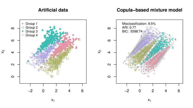
Figure 2: The artificial data set of Example 1.1 (left) and the contours of the fitted mixture of the bivariate mixture model with two Gumbel and two Clayton components and Normal marginal distributions (right).

∎

4.2 Bounded- and mixed-domain variables

The decoupling of the dependence properties from the marginal ones allows the easy construction of multivariate mixture models for bounded-domain data (like percentages or strictly positive variables).

Mixture models for such data are usually formed from component densities defined by the product of independent univariate densities of appropriate support. Those models imply that the univariate marginal distributions of the component densities are independent conditional on the component membership. In effect, such models attempt to capture the dependence in the data only through the mixing probabilities. For example, Dean and Nugent (2013) define multivariate Beta mixture models in this way, and use them highlighting that the implied conditional independence assumption can be rather restrictive in practice.

Under the current framework, models with more complex dependence can be defined by simply setting the component copula densities $c_{j}$ in (4), and choosing marginals with the required support.

More importantly, the current methodology can be used to construct multivariate mixture models for mixed-domain marginals. Example 4.2 below considers a mixture model with components that have seven Beta and one Gamma marginal distributions each.

Example 4.2:

Hoopdata.com is a website that was launched in 2009 and provides an extensive database for NBA statistics. We used Hoopdata.com’s database to gather data for the scoring behaviour of the $493$ NBA players that had more than $24$ minutes game time (which accounts for half a game played in full) in the 2011-2012 season. For each player, the data has observations for the season free throws percentage (“FTper”), the field goals percentage (“FGper”), the three point percentage (“ThreePper”), the percentage of field goals assisted, the percentage blocked, the percentage of “And1” field goals, and the total points scored in hundreds (“PointsHun”). The aim of the analysis is to form groups of players in terms of their performance.

For all players that had observation $0\%$ or $100\%$ in any of the percentages, the observation is replaced by $0.01\%$ and $99.99\%$, respectively. After making the substitutions, the free throws, the field goals and the three point percentages take values in $(0,1)$. Furthermore, the points scored are all positive. Plausible marginal specifications are a Beta distribution for modelling each of the percentage variables and a Gamma distribution for modelling the points scored. Then we use a 7-variate Gaussian copula for modelling the dependence between the 7 variables.

The multivariate Gaussian copula with correlation matrix $R$ is defined as

$$C^{(N)}(u_{1},\ldots,u_{p};R)=\Phi_{p}(\Psi(u_{1}),\ldots,\Psi(u_{p});R)\,,$$ (11)

where $\Phi_{p}(.,\ldots,.)$ is the distribution function of a standard $p$-variate Normal distribution with correlation matrix $R$ and $\Psi(.)=\Phi_{1}^{-1}(.)$ is the inverse distribution function of a standard Normal distribution. The matrix $R$ has the general form

$$R=\left[\begin{array}[]{cccc}1&\rho_{12}&\ldots&\rho_{1p}\\ \rho_{12}&1&\ldots&\rho_{2p}\\ \vdots&\vdots&\ddots&\vdots\\ \rho_{1p}&\rho_{2p}&\ldots&1\\ \end{array}\right]\,,$$ (12)

where $\rho_{tt^{\prime}}\in[-1,1]$ is the correlation between the $t$th and $t^{\prime}$th variable $(t,t^{\prime}\in\{1,\ldots,p\};t\neq t^{\prime})$.

For the current case the density of the mixture model to be fitted is

$$\sum_{j=1}^{k}\pi_{j}\phi_{7}\left[\Psi\left\{G_{j1}(x_{1})\right\},\ldots,\Psi\left\{G_{j7}(x_{7})\right\};R_{j}\right]\prod_{t=1}^{7}\frac{g_{jt}(x_{t})}{\phi_{1}[\Psi\{G_{jt}(x_{t})\}]}\,,$$ (13)

where $\phi_{p}$ is the density of a $p$-dimensional standard Normal distribution and $g_{jt}(x)=\partial{G_{jt}(x)}/\partial{x}$, where for $t\in\{1,\ldots,6\}$, $G_{jt}(x)$ is the distribution function of a Beta random variable with shape parameters $\alpha_{jt}$, and $G_{j7}(x)$ is the distribution function of a Gamma random variable with shape parameter $\kappa_{j}$ and scale $1/\lambda_{j}$. More specifically, the density functions for the marginals are

$$g_{jt}(z)=\left\{\begin{array}[]{ll}\displaystyle\frac{z^{\alpha_{jt}-1}(1-z)^{\beta_{jt}-1}}{B(\alpha_{jt},\beta_{jt})}\,,&t\in\{1,\ldots,6\}\\ \\ \displaystyle\frac{\lambda_{j}^{\kappa_{j}}}{\Gamma(\kappa_{j})}z^{\kappa_{j}-1}\exp(-\lambda_{j}z)\,,&t=7\end{array}\right.\quad(j=1,\ldots,k)\,.$$

The matrix $R_{j}$ has exactly the same structure as the matrix $R$ in (12) but the correlations depend on $j$ ensuring that each component in the mixture can accommodate different correlation structures. Hence, the parameters to be estimated are $\alpha_{j1}$, $\beta_{j1}$, $\ldots$, $\alpha_{j6}$, $\beta_{j6}$, $\kappa_{j}$ and $\lambda_{j}$ for the marginals of the $j$th component, $\rho_{12,j}$, $\ldots$, $\rho_{17,j}$, $\ldots$, $\rho_{67,j}$ for the copula of the $j$th component $(j=1,\ldots,k)$ and the mixing proportions $\pi_{1},\ldots,\pi_{k-1}$. Hence, the model in (13) has $q=36k-1$ free parameters. The number of free parameters can be further reduced by fitting models nested to (13) that have a structured correlation matrix. For example, a nested model to (13) with $16k-1$ parameters can be formed by considering exchangeable correlation for each component where all correlations appearing in $R_{j}$ are equal to $\rho_{j}$ $(j=1,\ldots,k)$.

For $k=2,\ldots,9$, density (13) is fitted to the data on the NBA players with both unstructured and exchangeable correlation. For the models with exchangeable correlation and for each $k$, $15$ sets of starting values were obtained by selecting $15$ sets of $k$ randomly selected observations for the intialization of the component-wise IFM procedure in Subsection 3.2.2. Then the model with the highest log-likelihood was chosen and was also used to initialise the model with unstructured correlation.

Furthermore, we restricted the variance of each of the Beta marginals involved in the mixture to be greater than $10^{-4}$. In this way, unbounded likelihood values relating to observations with the same percentage value can be avoided.

Table 2 lists the maximized log-likelihood, the number of parameters $q$ and the BIC value for the best $18$ fitted mixtures. The model with exchangeable correlation matrix and $k=6$ has the lowest BIC value.

k	Log-likelihood	$q$	BIC		Log-likelihood	$q$	BIC
	Exchangeable correlation				Unstructured correlation
$1$	$2414.56$	$15$	$-4736.12$		$2614.84$	$35$	$-5012.65$
$2$	$3146.45$	$31$	$-6100.68$		$3491.12$	$71$	$-6542.00$
$3$	$3734.31$	$47$	$-7177.19$		$3990.00$	$107$	$-7316.55$
$4$	$3900.49$	$63$	$-7410.34$		$4119.53$	$143$	$-7352.40$	($\star$)
$5$	$4002.73$	$79$	$-7515.62$		$4218.24$	$179$	$-7326.59$
$6$	$4053.61$	$95$	$-7518.17$	($\star$$\star$)	$4267.97$	$215$	$-7202.83$
$7$	$4073.36$	$111$	$-7458.47$		$4270.47$	$251$	$-6984.62$
$8$	$4146.57$	$127$	$-7505.68$		$4365.99$	$287$	$-6952.43$
$9$	$4159.01$	$143$	$-7431.35$		$4387.43$	$323$	$-6772.09$

Table 2: Maximum likelihood fits of the density (13) for the data on the NBA players with $k\in\{2,\ldots,9\}$ components for both unstructured and exchangeable correlation structure. A ($\star$) denotes the best BIC for each copula specification and a ($\star\star$) the best BIC overall.

The maximum of the weights $w_{i1},\ldots,w_{ik}$ at the last iteration of the EM algorithm (see step E1 in 3.1) is used to determine the cluster membership of each observation. For the model with exchangeable correlation matrices and $k=6$, Figure 3 shows the marginal histograms of the observations within each cluster along with the marginal densities $g_{jt}(.)$ at the maximum likelihood estimates for each cluster-variable combination. The agreement of the fitted marginals with the histograms of the variables indicates a good fit. Furthermore, Figure 3 shows that the fit has achieved some separation between the clusters, especially for “PointsHun”.

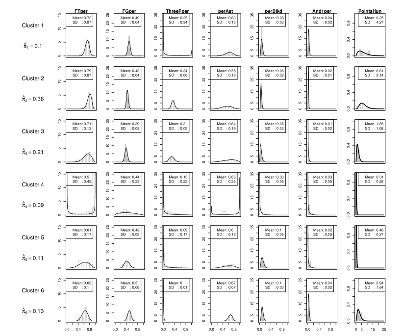
Figure 3: Mixture of $6$ $7$-dimensional Gaussian copulas with exchangeable correlation matrices and $6$ Beta and $1$ Gamma marginals each. The plots show the marginal histograms of the observations within each cluster along with the fitted marginal densities for each cluster-variable combination. The fitted mixing proportions $\hat{\pi}_{i}$ $(i=1,\ldots,6)$ are also reported.

A “true classification” of the players in terms of performance is not generally available, so it is hard to check how good the resultant classification is. However, there is a wealth of metrics that attempt to capture different characteristics of the player. A few representative metrics include the NBA Efficiency rating (“EFF”), the Usage Rate (“USG”), the True Shooting percentage (“TSper”), John Hollinger’s Player Efficiency Rating (“PER”) and Alternative Win Score (“AWS”). Hoopdata.com provides the values for these metrics for each player in the 2011-2012 season and we use these values to assess the comparative performance of the copula-based mixture model to that of a Normal mixture fitted using the mclust (Fraley et al., 2012) R package as follows: each metric is broken into $I$ intervals, whose endpoints are calculated using the empirical quantiles at $I+1$ equidistant probabilities ranging from $0$ to $1$. For each metric and for $I\in\{2,\ldots,30\}$, we calculate the ARI of the clustering with 6 Beta and 1 Gamma marginal, and the ARI of the clustering from the Normal mixture model with the lowest BIC ($4$ components with VEV parameterization with BIC $-5026.44$; VEV stands for “variable volume, equal shape, variable orientation” and characterizes a particular parameterization for the variance-covariance matrix of the multivariate Normal distribution for the component distributions; see, Fraley et al. 2012 for the VEV and the other parameterizations that mclust uses). Figure 4 shows the results for each metric. Despite the low ARI’s for both fits, all points fall below the $45^{o}$ line and, hence, the clustering from the copula-based mixture model clearly dominates the one from the optimal Normal mixture model with regards to those metrics.

Figure 4: Clustering quality of best copula-based mixture model versus the best Normal mixture model. The dashed line is the $45^{o}$ line from the origin.

As a reviewer correctly pointed out, another way to handle clustering of bounded- or mixed-domain data is to first appropriately transform the data and then use standard mixture models for continuous data, such as Normal mixtures. Dean and Nugent (2013) consider such an approach by taking the arcsine transformation of data in $[0,1]$ and then fitting Normal mixture models on the transformed data. Their results indicate that treating the bounded-domain data with distributions that are defined on that domain produces better results (see, for example Dean and Nugent, 2013, Table 1, for the results of the simulation study). Another important reason for working with the bounded-domain data directly is for avoiding the arbitrariness of choice of transformation before fitting a mixture model. Section 1 of the supplementary material extends Example 4.2 to illustrate that distinct sensible, transformations can lead to different results.

4.3 Real-valued variables

4.3.1 Invariance with respect to affine transformations

Suppose that the $n$ vectors ${\bm{x}}_{1},\ldots,{\bm{x}_{n}}$ of observations have real-valued components. Then, the fit of a copula-based mixture model with marginal distributions in the location-scale family (like Normal, skew-Normal, Cauchy, t, logistic and so on) is invariant with respect to the translation and component-wise scaling of ${\bm{x}}_{1},\ldots,{\bm{x}}_{n}$. This is because the location and scale of the components are determined only by the marginal distributions.

More formally, suppose that all marginals support the real line and that the fitted marginal means and variances of the $j$th component based on data ${\bm{x}}_{1},\ldots,{\bm{x}}_{n}$ are $\hat{\mu}_{j1},\ldots,\hat{\mu}_{jp}$ and $\hat{\sigma}^{2}_{j1},\ldots,\hat{\sigma}^{2}_{jp}$ $(j=1,\ldots,k)$, respectively. Then, if ${\bm{z}}_{i}=a+B{\bm{x}}_{i}$ $(i=1,\ldots,n)$, where $B$ is a diagonal matrix with non-zero diagonal entries, the fitted marginal means and variances of the $j$th component based on data ${\bm{z}}_{1},\ldots,{\bm{z}}_{n}$ will simply be $a+B_{11}\hat{\mu}_{j1},\ldots,a+B_{pp}\hat{\mu}_{jp}$ and $B_{11}^{2}\hat{\sigma}^{2}_{j1},\ldots,B_{pp}^{2}\hat{\sigma}^{2}_{jp}$ $(j=1,\ldots,k)$, respectively. This follows directly from the invariance properties of the maximum likelihood estimator.

However, depending on the choice of copulas, the same mixture will generally produce a different clustering for general affine transformations of the form $z^{i}=a+Bx^{i}$ $(i=1,\ldots,n)$, where $B$ is a general real-valued $p\times p$ matrix. This is because a copula-defined distribution is not necessarily closed under general affine transformations (for example rotations). In contrast closure under general affine transformations is satisfied for all mixture models that are based on elliptical distributions such as Normal and $t$ mixtures (Fang et al., 2002).

4.3.2 Rotated copulas

In two dimensions, the survival version of any copula $C(u_{1},u_{2})$ is $C_{180}(u_{1},u_{2})=u_{1}+u_{2}-1+C(u_{1},u_{2})$, where “180” denotes that the survival copula is a rotated version of $C(u_{1},u_{2})$ by $180^{o}$ clockwise. Similarly, counter-clockwise rotated versions of $C(u_{1},u_{2})$ by $90^{o}$ and $270^{o}$ can be defined as functions of $C(u_{1},u_{2})$ and $u_{1}$, $u_{2}$. Expression for those are given in Brechmann and Schepsmeier (2013). Hence, one can select an initial dictionary of copulas to be used and then to further enrich this dictionary with the rotated versions of the copulas.

Example 4.3:

In Example 4.1 we chose the copulas for the components by recognising the need for mixture components that can accommodate extreme tail dependence through inspection of the scatterplot of the data. In this respect, we chose to have two mixture components based on the Gumbel copula which exhibits upper tail dependence and two components based on the Clayton copula which exhibits lower tail-dependence. Since a rotated version of the Clayton copula by $180^{o}$ (survival Clayton) would exhibit upper tail dependence one might argue that a mixture model that uses the rotated version of the Clayton instead of Gumbel would have produced a fit of comparable quality. Indeed that is the case; fitting a model with two Clayton and two survival Clayton components gives misclassification error of $9.875\%$ and a BIC value of $5561.73$. Similarly, fitting a model with two Gumbel and two survival Gumbel components gives misclassification error of $11.25\%$ and a BIC value of $5644.36$. ∎

As is illustrated in Example 4.3, the ability to construct new copula families from known ones certainly adds great flexibility when constructing copula-based mixture models for clustering. However, it certainly does not simplify model selection in a mixture model framework; if we limit ourselves to a dictionary of $d$ copulas, then for finding the best model amongst the models with $k$ components we need to fit and select the best model from $\binom{d+k-1}{k}$ models. Furthermore, if the number of components is also considered as part of the model selection exercise, then one needs to fit and compare $\sum_{k=1}^{K}\binom{d+k-1}{k}$ where $K$ is a preset maximum number of components. Both these numbers increase quickly as either $K$ or $d$ increase possibly making the model selection exercise impractical.

4.3.3 Component-wise parametric rotations

Subsections 4.3.1 and 4.3.2 show that the added flexibility from the use of mixture of copulas may come with the price of two shortcomings from a practitioners point of view: the general lack of invariance with respect to general affine transformations of the data, and the fact that completely different copulas can result in fits of comparable quality. The latter issue is not so serious provided that the computational resources are enough for fitting many models and keeping in mind the target of the analysis is to find a good model. Though it certainly points towards the direction that if one had a more flexible specification for the mixture components, the number $\sum_{k=1}^{K}\binom{d+k-1}{k}$ of models that need to be fitted is significantly decreased because $d$ can be drastically reduced. The invariance issue is harder to tackle. However, a flexible enough model could alleviate some of the invariance issues by maintaining the translation and scaling invariance of the component densities, and by allowing the component densities to rotate based on the observations.

Consider the mixture of copulas specified by (1) and (2) with $p=2$. Temporarily omitting the component index, each component density has the form

$$f({\bm{x}}^{*};{\bm{\gamma}},{\bm{\psi}})=c(G_{1}(x_{1}^{*};{\bm{\gamma}}_{1}),G_{2}(x_{2}^{*};{\bm{\gamma}}_{2});{\bm{\psi}})g_{1}(x_{1}^{*};{\bm{\gamma}}_{1})g_{2}(x_{2}^{*};{\bm{\gamma}}_{2})\,,\quad{\bm{x}}^{*}\in\Re^{2}\,.$$

Now consider the transformation ${\bm{X}}=O(\omega){\bm{X}}^{*}$, where $O(\omega)$ is the rotation matrix

$$O(\omega)=\left[\begin{array}[]{cc}\cos\omega&-\sin\omega\\ \sin\omega&\cos\omega\\ \end{array}\right]\,,$$

with $\omega\in(0,2\pi]$. Then ${\bm{X}}$ is a counter-clockwise rotation of ${\bm{X}}^{*}$ at an angle $\omega$ and the density function of ${\bm{X}}$ is simply

$$f^{*}({\bm{x}};{\bm{\gamma}},{\bm{\psi}},\omega)=f(O(\omega)^{\top}{\bm{x}};{\bm{\gamma}},{\bm{\psi}})\,,\quad{\bm{x}}\in\Re^{2}\,,$$ (14)

because for any rotation matrix $O(\omega)^{-1}=O(\omega)^{\top}$ ($O(\omega)$ is orthonormal) and $|\det O(\omega)|=1$. Hence, the contours of $f^{*}$ will be a counter-clockwise rotation of the contours of $f$ at an angle $\omega$. Hence, in the two-dimensional case, an extended mixture model can be defined that has the form

$$h({\bm{x}};{\bm{\theta}},{\bm{\omega}})=\sum_{j=1}^{k}\pi_{j}f^{*}_{j}({\bm{x}};{\bm{\gamma}}_{j},{\bm{\psi}}_{j},{\bm{\omega}}_{j})\,.$$ (15)

The difference of the latter specification from the mixture model in (1) and (2) is that there are an extra $k$ rotation angles to be estimated, but the added flexibility is enormous. The practitioner can now select the marginals and a much smaller dictionary of copulas; notice that all versions of the rotated copulas by $90^{o}$, $180^{o}$ and $270^{o}$ are special cases for the components of model (15) for specific values of $\omega_{1},\ldots,\omega_{k}$ and that other exotic bivariate distributions may result for arbitrary angles.

The mixture model (15) can be fitted using the EM algorithm; the only modification from the general iteration in Subsection 3.1 is that at M-step 2 of the $\ell$th iteration, the function

$$\sum_{j=1}^{k}\sum_{i=1}^{n}w_{ij}^{(\ell+1)}\left[\log c_{j}(G_{1}(z_{i1}(\omega_{j});{\bm{\gamma}}_{j1}),\ldots,G_{p}(z_{ip}(\omega_{j});{\bm{\gamma}}_{jp});{\bm{\psi}}_{j})+\sum_{t=1}^{p}\log g_{t}(z_{it}(\omega_{j});{\bm{\gamma}}_{jt})\right]\,,$$ (16)

is maximized with respect to ${\bm{\gamma}}_{11},\ldots,{\bm{\gamma}}_{1p},\ldots,{\bm{\gamma}}_{k1},\ldots,{\bm{\gamma}}_{kp},{\bm{\psi}}_{1},\ldots,{\bm{\psi}}_{k},\omega_{1},\ldots,\omega_{k}$. In (16), ${\bm{z}}_{i}(\omega_{j})=O(\omega_{j})^{\top}{\bm{x}}_{i}$ where ${\bm{z}}_{i}(\omega_{j})=(z_{i1}(\omega_{j}),\ldots,z_{ip}(\omega_{j}))^{\top}$ $(i=1,\ldots,n;j=1,\ldots,k)$. This M-step can also be broken down into $k$ independent optimizations.

In order to avoid maximization over a large parameter space, the ECM algorithm in Subsection 4.1 can be extended for handling parametric rotations i) by replacing $x_{it}$ with $z_{it}(\omega_{j}^{(\ell)})$ $(t=1,\ldots,p)$ in CM-step 1 and CM-step 2, and ii) by including an additional last step to update the angles at the values of the marginal and copula parameters from CM-step 1 and CM-step 2. In that last step the objective

$$\sum_{j=1}^{k}\sum_{i=1}^{n}w_{ij}^{(\ell+1)} \Bigg{[}\log c_{j}(G_{1}(z_{i1}(\omega_{j});{\bm{\gamma}}^{(\ell+1)}_{j1}),\ldots,G_{p}(z_{ip}(\omega_{j});{\bm{\gamma}}^{(\ell+1)}_{jp});{\bm{\psi}}^{(\ell+1)}_{j})$$ (17)

$$+ \sum_{t=1}^{p}\log g_{t}(z_{it}(\omega_{j});{\bm{\gamma}}^{(\ell+1)}_{jt})\Bigg{]}\,,$$

is maximized with respect to $\omega_{1},\ldots,\omega_{k}$ to obtain updated values $\omega_{1}^{(\ell+1)},\ldots,\omega_{k}^{(\ell+1)}$. As is the case for CM-step 1 and CM-step 2, this last step can also be broken down into parallel optimizations across components, each of which consists of a one-dimensional maximization with respect to the respective angle.

Example 4.4:

As is illustrated in Example 4.3 one can fit a mixture of two Clayton and two survival Clayton, or a mixture of two Gumbel and two survival Gumbel, or a mixture of two Gumbel and two Clayton copulas to the artificial data of Example 1.1 and obtain comparable fits in all cases. Hence, we have considered the combinations of four different copulas for the components so far. The whole modelling exercise is much easier if we pick just one copula which exhibits tail-dependence (upper or lower), and Normal marginals and use those for setting up the mixture density (15).

For example, using the Clayton copula one obtains the estimated angles $\hat{\omega}_{1}=180.41$, $\hat{\omega}_{2}=180.78$, $\hat{\omega}_{3}=7.13$, $\hat{\omega}_{4}=359.99$ and a misclassification error of $9.875\%$. Figure 5 shows the contours of the fitted component densities across the iterations of the ECM algorithm and demonstrates the enormous flexibility that parametric rotations offer when setting copula-based mixture models. Iteration 0 (top left) refers to the starting values for the ECM algorithm.

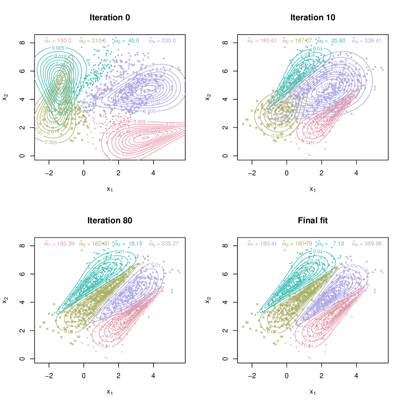
Figure 5: The contours of the fitted component densities across the iterations of the ECM algorithm when allowing for parametric rotations. The value of the component angles at the depicted iterations is given in the top of each plot. Iteration 0 (top left) refers to the starting values for the ECM algorithm.

The BIC value for the fit that allows parametric rotations is $5585.372$ which is larger the $5561.73$ of the mixture with two Clayton and two survival Clayton in Example 4.3. This slight inflation is due to the 4 extra parameters included in the model that allows for component-wise parametric rotations. ∎

4.3.4 Identifiability of rotations for elliptical distributions

It should be noted that when at least one of the component distributions is elliptical then the corresponding angles in (15) are not identifiable. To show that, suppose that ${\bm{X}}^{*}$ has density $f({\bm{x}}^{*};{\bm{\gamma}},{\bm{\psi}})$ with mean ${\bm{\mu}}^{*}$ and variance-covariance matrix $\Sigma^{*}$. If ${\bm{X}}$ has density (14), the variance-covariance matrix of ${\bm{X}}$ is

$${\rm Var}({\bm{X}}) =E_{f^{*}}\left[\left\{{\bm{X}}-{\bm{\mu}}(\omega)\right\}\left\{{\bm{X}}-{\bm{\mu}}(\omega)\right\}^{\top}\right]$$

$$=E_{f}\left\{O(\omega)({\bm{X}}^{*}-{\bm{\mu}}^{*})({\bm{X}}^{*}-{\bm{\mu}}^{*})^{\top}O(\omega)^{\top}\right\}$$

$$=O(\omega)\Sigma^{*}O(\omega)^{\top}\,.$$

The variance-covariance matrix $\Sigma^{*}$ admits the eigen-decomposition $\Sigma^{*}=Q_{j}\Lambda_{j}Q_{j}$ where $Q_{j}$ is an orthogonal matrix. Noting that the product of two-orthogonal matrices is orthogonal $O(\omega)\Sigma^{*}O(\omega)$ is also a variance covariance-matrix and given that we can only identify variances and covariances, the angle $\omega$ is not identifiable. For example, if Normal marginals are considered, then using a Gaussian copula for one of the components of (15) will result to identifiability issues.

4.3.5 Local rotation unidentifiability for general copulas

Furthermore, as is discussed in Nelsen (2006, Section 4.3), many Archimedean copulas have the product copula $C(u,v)=uv$ as a special case for specific values of their parameters (for example, the Clayton copula for $\psi\to 0$, the Gumbel for $\psi\to 1$, the Frank for $\psi\to 0$, and so on). The use of parametric rotations poses local identifiability problems, for those specific boundary values of the copula parameter.

5 Closure under marginalization

A desirable property that well-used mixture models such as mixtures of multivariate Normal, multivariate skew-Normal and multivariate skew-t distributions share is closure under marginalization. Such a property guarantees that the marginal of any dimension of the component distributions belongs to the same family of distributions as the component distribution itself, and allows the easy transition from the full mixture model to a marginal model of any order. For example, one can fit a mixture of multivariate Normal distributions and then plot the contours of all bivariate marginal densities by using the bivariate Normal density and the appropriate subsets of parameters from the full model without the need of integrating over the fitted density.

For $m<p$ and continuous random variables the requirement of closure under marginalization for the component density is that if

$$f_{j}^{(m)}(x_{1},\ldots,x_{m};\theta_{j})=\int_{\mathcal{X}_{m+1}}\ldots\int_{\mathcal{X}_{p}}f_{j}(x_{1},\ldots,x_{p};\theta_{j})dx_{m+1}\ldots dx_{p}\quad(j=1,\ldots,k)\,,$$

where $\mathcal{X}_{m+1},\ldots,\mathcal{X}_{p}$ are the supports of the random variables $X_{m+1},\ldots,X_{p}$, respectively, then $f_{j}^{(m)}$ has exactly the same functional form as the $p$ dimensional density $f_{j}$ does but in $m$ dimensions. For a copula-defined $p$-dimensional component density the requirement from the copula distribution is that, if

$$C_{j}^{(m)}(G_{1}(x_{1};\gamma_{j1}),\ldots,G_{m}(x_{m};\gamma_{jm});\psi_{j})=C_{j}(G_{1}(x_{1};\gamma_{j1}),\ldots,G_{m}(x_{m};\gamma_{jm}),1,\ldots,1;\psi_{j})\,,$$

then $C_{j}^{(m)}$ belongs to the same family of copulas as $C_{j}$ does. To derive this requirement, marginalization is performed by setting $x_{m+1},\ldots,x_{p}$ to the maximum of their range of definition. This property is satisfied for all elliptical copulas like the Gaussian copula and the $t$-copula (see Fang et al., 2002, for results on the family of elliptical copulas). Furthermore, closure under marginalization holds for every Archimedean and nested Archimedean copula, because its generator function necessarily takes value 0 at 1 (see, for example, Hofert et al., 2012, for definitions and results for multivariate Archimedean and nested Archimedean copulas).

The results here extend to the case of discrete data by replacing the integration of density functions with summations of probability mass functions of the form (3). Closure under marginalization is a particularly relevant property to be satisfied when building mixture models for discrete data, because, otherwise, the computational burden involved in the calculation of marginals of the mixture model can be prohibitive.

A class of copulas that does not satisfy the property of closure under marginalisation is the class of vine copulas (see, for example, Bedford and Cooke 2002).

Example 5.1:

In Example 4.2, the mixture components were defined using the Gaussian copula. Hence, the bivariate marginal density of $X_{t}$ and $X_{s}$ $(s,t=1,\ldots,7;s\neq t)$ corresponding to the density (13), are simply

$$\sum_{j=1}^{k}\pi_{j}\phi_{2}\left[\Psi\left\{G_{js}(x_{s})\right\},\Psi\left\{G_{jt}(x_{t})\right\};R_{j,st}\right]\frac{g_{js}(x_{s})g_{jt}(x_{t})}{\phi_{1}[\Psi\{G_{js}(x_{s})\}]\phi_{1}[\Psi\{G_{jt}(x_{t})\}]}\,,$$ (18)

where $R_{j,st}$ is the $2\times 2$ correlation matrix with the $(s,s)$th and $(t,t)$th components of $R_{j}$ in the diagonal and the $(s,t)$th component of $R_{j}$ in the off-diagonal $(j=1,\ldots,k)$.

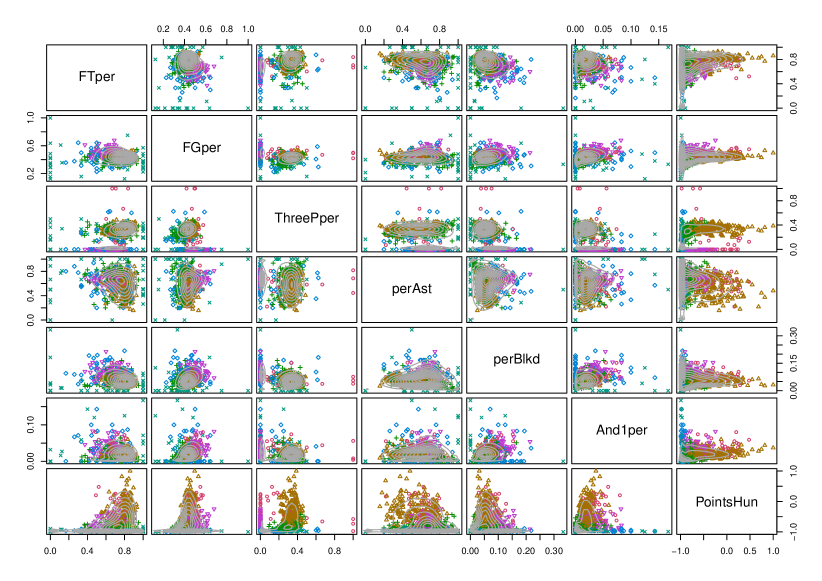
Figure 6: The contours of all the bivariate marginal densities of the mixture model with $6$ components and unstructured correlation matrices from Example 4.2. The observations are coloured according to their assigned cluster.

Figure 6 shows the contours of the bivariate marginals for the best model according to BIC in Table 2, with the data coloured according to their assigned cluster. ∎

6 Discrete data

6.1 Copula-based mixture models

The general mixture model specification and fitting framework set in Section 2 and Section 3 can directly be used for constructing and estimating mixture models with discrete marginal distributions. Nevertheless, in the discrete case, model specification and estimation need a more careful consideration than they do in the continuous case.

6.2 Model specification

The choice of the component copulas cannot be based entirely on dependence considerations (tail dependence, correlation, and so on) as is rather intuitively done in the continuous case. This is because the copula alone does not anymore characterize the dependence between the discrete marginals; the usual dependence measures, like Kendall’s $\tau$ and Spearman’s $\rho$, are not margin-free as they are in the continuous setting. Genest and Nešlehová (2007, §4) provide theoretical derivations and demonstrations of such issues, with detailed discussions of how they reflect in practice. Furthermore, as discussed in Section 5 and as is illustrated by Example 6.1 below, closure under marginalization is particularly relevant for mixture models for discrete data, if marginal assessments of the clustering or fit are to be obtained.

6.3 Estimation

For the analysis of discrete data, M-step 2 of Subsection 3.1 takes the form

• M-step 2: Maximize the log-likelihood

  $$\sum_{j=1}^{k}\sum_{i=1}^{n}w_{ij}^{(\ell+1)}\left[\log\sum_{{\bm{d}}_{i}}\mathop{\rm sgn}({\bm{d}}_{i})C(G_{1}(d_{i1};{\bm{\gamma}}_{j1}),\ldots,G_{p}(d_{ip};{\bm{\gamma}}_{jp});{\bm{\psi}}_{j})\right]\,,$$ (19)

with respect to ${\bm{\psi}}_{1},\ldots,{\bm{\psi}}_{k},{\bm{\gamma}}_{11},\ldots,{\bm{\gamma}}_{1p},{\bm{\gamma}}_{k1},\ldots,{\bm{\gamma}}_{kp}$, where ${\bm{d}}_{i}$ is as in expression (3) for an observation ${\bm{x}}_{i}$ $(t=1,\ldots,p;j=1,\ldots,k;i=1,\ldots,n)$. Note here that in the discrete case the ECM algorithm would offer no simplification over EM, since a copula-specified probability mass function cannot be decomposed as in the continuous case.

The combination of $\sum_{t=0}^{p}\binom{p}{t}$ summation terms in the right-most summation in (19) and the lack of closed-form expression for general copulas can result in the accumulation of numerical error that in turn can lead in calculated probability mass functions less than $0$ or greater than $1$ for certain parameter settings, which can result in computational problems in the M-step.

A partial resolution of those issues, at least for small to moderate $p$, exists for copulas that are derived from well-known distribution functions through the inverse probability transform. Let $C(u_{1},\ldots,u_{p})=H(H_{1}^{-1}(u_{1}),\ldots,H_{p}^{-1}(u_{p}))$, where $H(.,\ldots,.)$ is some $p$-variate distribution function with marginals $H_{1}(.),\ldots,H_{p}(.)$ and $H_{j}^{-1}(.)$ is the quantile function of $H_{j}(.)$ $(j=1,\ldots,p)$. Then, omitting the component index and suppressing the dependence on the parameters,

$$\sum_{{\bm{d}}}\mathop{\rm sgn}({\bm{d}})C(G_{1}(d_{1}),\ldots,G_{p}(d_{p}))=\int_{D(x_{1})}\ldots\int_{D(x_{p})}h(y_{1},\ldots,y_{p})dy_{p}\ldots dy_{1}\,,$$ (20)

where $D(x_{t})$ is the interval from $H_{t}^{-1}\{G_{t}(x_{t}-1)\}$ to $H_{t}^{-1}\{G_{t}(x_{t})\}$ $(t=1,\ldots,p)$, and $h(.,\ldots,.)$ is the density function corresponding to $H(.,\ldots,.)$.

Hence, a single evaluation of the rectangle probability in (20) is sufficient for calculating the probability mass function. For special but prominent copulas like the Gaussian and the $t$ copula and for not very large $p$, the probability mass function can be calculated through accurate approximation methods like those of Joe (1995). Such methods are implemented in the mprobit R package by Joe, Choy and Zhang and the mvtnorm R package (Genz et al., 2013). The following example concerns the use of copulas to construct mixtures of trivariate Binomial distributions that allow for dependence.

Example 6.1:

This example relates to cognitive diagnosis modelling. The data set consists of the responses of 536 middle school students on 20 items of a fraction subtraction test. Each item can belong to more than one attribute that one wants to measure. Hence, attribute scores for each student can be obtained by counting the number of successful items out of the total items that belong to each attribute. The data are available in the CDM R package (Robitzsch et al., 2014) and its documentation describes which items belong to which attribute. The aim of this example is to use some of the attribute scores of the students for the construction of performance clusters of the latter. The scores that are used in this example are for the attributes “separate a whole number from a fraction” (score $X_{1}$), “borrow from whole number part” (score $X_{2}$) and “subtract numerators” (score $X_{3}$), which are traced on 13, 8 and 19 items, respectively. Hence, a natural distributional choice for each of $X_{1}$, $X_{2}$ and $X_{3}$ is Binomial. More specifically, we assume that for the $j$th component, the $t$th marginal distribution is Binomial with index $m_{j}$ and probability of success $p_{jt}$ $(t=1,2,3;j=1,\ldots,k)$, where $m_{1}=13$, $m_{2}=8$ and $m_{3}=19$.

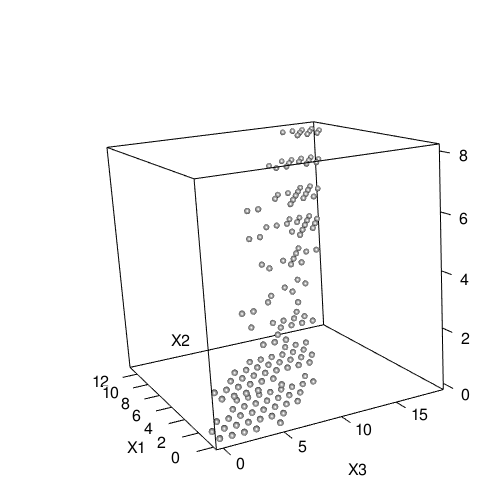
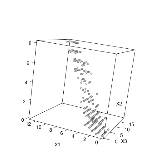
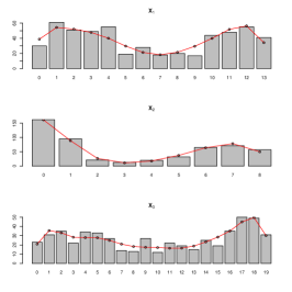
Figure 7: Different views of the three attribute scores for all students. The barplot at the rightmost plot shows the observed (bars) and the fitted (points) frequencies for the three attributes based on the selected model.

Figure 7 presents the data from two different angles and reveals that there is strong positive association between each pair of attribute scores. This is because the three attributes share items, and this association needs to be taken into account when clustering the students. The barplot at the rightmost plot shows the observed (bars) and the fitted (points) frequencies for the three attributes based on the selected model. Such data have also been analysed in the past via mixture models (see, Dean and Nugent, 2013) but only after transforming the scores into percentages and treating those as realizations of continuous random variables. Such transformations are not necessary when using copula-based mixture models; to accommodate for the apparent association, we construct $4$ different families of mixture models each with components that are trivariate Binomial distributions defined using i) one-parameter Frank copulas, ii) two-parameter Frank copulas (see, Zimmer and Trivedi, 2006), iii) trivariate Gaussian copulas as in (11) with unstructured correlation (one parameter each), and iv) trivariate Gaussian copulas with exchangeable correlation (three parameters each). Note here that defining multivariate Binomial distributions which allow for correlated marginals is not straightforward outside the copula framework (for a discussion on bivariate and multivariate Binomial distributions, see Johnson et al., 1997).

	One-parameter Frank				Gaussian - exchangeable correlation
$k$	Log-likelihood	$q$	BIC		Log-likelihood	$q$	BIC
1	-5899.71	4	11824.56		-5063.32	4	10151.78
2	-3098.11	9	6252.78		-3049.76	9	6156.08
3	-2843.22	14	5774.42		-2846.08	14	5780.14
4	-2758.64	19	5636.68		-2750.57	19	5620.54
5	-2720.35	24	5591.52		-2707.63	24	5566.08
6	-2693.26	29	5568.76	($\star$)	-2679.56	29	5541.36	($\star$$\star$)
7	-2678.67	34	5570.99		-2669.90	34	5553.45
8	-2666.62	39	5578.32		-2662.46	39	5570.00
	Two-parameter Frank				Gaussian - unstructured correlation
$k$	Log-likelihood	$q$	BIC		Log-likelihood	$q$	BIC
1	-5897.92	5	11827.261		-5010.11	6	10057.925
2	-3085.49	11	6240.11		-2990.15	13	6061.99
3	-2825.91	17	5758.65		-2773.45	20	5672.58
4	-2750.89	23	5646.32		-2709.79	27	5589.26
5	-2711.81	29	5605.86		-2674.92	34	5563.50	($\star$)
6	-2673.79	35	5567.52	($\star$)	-2671.35	41	5600.35
7	-2659.98	41	5577.60		-2662.37	48	5626.38
8	-2654.7	47	5604.76		-2658.42	55	5662.47

Table 3: Results from fitting finite mixtures with different number of components. A ($\star$) denotes the best BIC for each copula specification and a ($\star\star$) the best BIC overall.

The one-parameter Frank copula is defined as

$$C^{(F)}(u_{1},u_{2},u_{3};\psi)=-\frac{1}{\psi}\log\left\{1+\frac{(\exp^{-\psi u_{1}}-1)(\exp^{-\psi u_{2}}-1)(\exp^{-\psi u_{3}}-1)}{(\exp^{-\psi}-1)^{2}}\right\}\,,$$ (21)

where $\psi$ is an association parameter which is common for all marginals, implying symmetric dependence. The two-parameter Frank copula is a trivariate nested Archimedean copula which has been used in the applications in Zimmer and Trivedi (2006) and is defined as

$$C^{(F^{*})}(u_{1},u_{2},u_{3};{\bm{\psi}})=\\ -\frac{1}{\psi_{1}}\log\left[1-\frac{1}{\gamma_{1}}\left\{1-\big{(}1-\frac{1}{\gamma_{2}}\tau_{1}\tau_{2}\big{)}^{\psi_{1}/\psi_{2}}\right\}(1-\exp(-\psi_{1}u_{3}))\right]\,,$$ (22)

where $0<\psi_{1}<\psi_{2}$, $\zeta_{1}=1-\exp(-\psi_{1})$, $\zeta_{2}=1-\exp(-\psi_{2})$, $\tau_{1}=1-\exp(-\psi_{2}u_{1})$ and $\tau_{2}=1-\exp(-\psi_{2}u_{2})$. The two-parameter Frank copula has (21) as a special case, and with one extra parameter it allows for partial symmetry capturing more flexible associations between the marginals.

Since (21) and (22) are of closed-form, the calculation of the probability mass function for the components of the respective mixture models is performed using (3), which in the current case of $3$ variables consists of $8$ terms. For the multivariate Gaussian copula, the probability mass functions for the components are instead obtained via the approximation of the rectangle probability in (20) using the mprobit R package. In order to avoid overflows due to the approximation of the multivariate Normal integral, probabilities calculated as smaller than $10^{-12}$ were kept to this value.

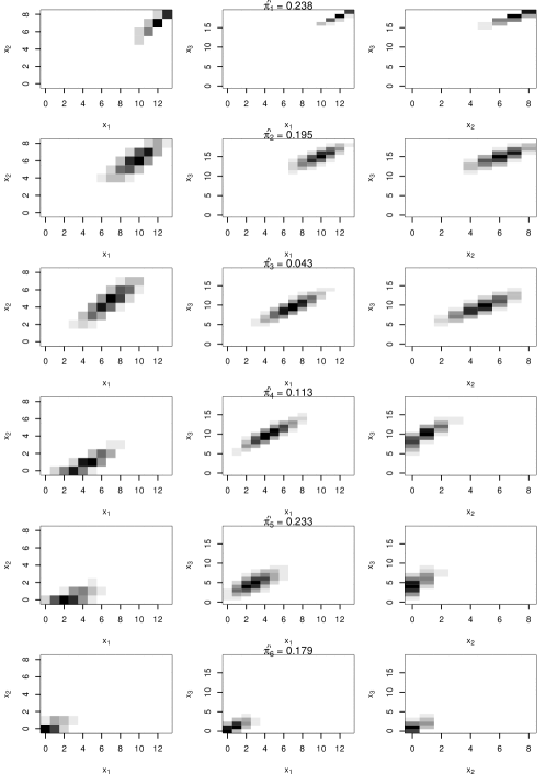
Figure 8: Fitted components from the model with the selected model with Gaussian copula with exchangeable correlation and 6 components.

The finite mixture given in (1) was fitted using the EM algorithm of Section 3.1, where now ${\bm{\theta}}_{j}=(\bm{\psi}_{j},p_{j1},p_{j2},p_{j3})$ $(j=1,\ldots,k)$. Starting values were obtained using the approach described in Subsection 3.2.2 with 10 sets of random starting values. In parallel to that the following sequential approach has been applied: for $k=1$, estimates for the Binomial proportions were obtained by the marginals, while the correlation parameters were set equal to the sample counterparts or their average in the cases when one correlation parameter is used for all pairs. For the two-parameter Frank copula, one parameter was set equal to the smallest of the three correlations and the other to the same value plus a small positive number in order to satisfy the restriction $\psi_{1}<\psi_{2}$. Then starting values for the model with $k+1$ components were obtained by using the parameters of the model with $k$ components and by adding a new component with parameter values those found when fitting a model with just one component. This new component was given a small mixing proportion (we used 0.05). This procedure worked well and provided the largest maximized log-likelihood for almost all $k$.

Table 3 shows the results from fitting a series of models. The maximized log-likelihood, the number of parameters $q$ and the value of BIC are reported for each model. The overall best model according to BIC is noted with ($\star\star$) and is the model with 6 components specified using Gaussian copulas with exchangeable correlation.

The Gaussian copula is closed under marginalisation and this allows the effortless calculation of bivariate marginals (see Section 5 for details). Each row of Figure 8 corresponds to one of the fitted trivariate Binomial components, and shows the $3$ possible bivariate marginals of that component. The label of each row gives the corresponding mixing proportion. The darker the color on each plot the larger is the probability mass for the corresponding combination of values of the Binomial variables. The component in the first row corresponds to the students that scored very well in the test in all attributes, and the component in the last to those with the worst results. As is apparent in the plots of Figure 8, there is a strong positive correlation in most of the components, which implies a general ability of different levels in all three attributes. A few components deviate from this pattern. For example, the component in the fourth row from the top corresponds to students that scored poorly in $X_{1}$ and $X_{2}$ but moderately in $X_{3}$. Also, the component in the fifth row from the top corresponds to students whose scores for $X_{1}$ and $X_{2}$ are very close to $0$ and the scores for $X_{3}$ are slightly higher. Lastly, the barplot in Figure 7 shows that the selected model fits satisfactorily the observed frequencies, despite the rather complicated behaviour they demonstrate.

7 Discussion and further work

7.1 Advantages

This paper introduces a general framework for model-based clustering where the component densities can be specified through copulas.The numerous examples in this paper both on real and artificial data illustrate the great flexibility that this framework offers.

For continuous data, Sklar’s theorem ensures that the copula fully describes the dependence structure separately from any marginal properties; this allows the construction of a bivariate mixture model in Example 4.1 that has Normal marginals and can accommodate extreme tail dependence in the clusters. Such flexibility allows the construction of mixture models that are capable of producing a variety of exotic shapes (for example, star-shaped or banana-shaped clusters), that are far from the cluster shapes that are supported from contemporary proposals in the literature.

For discrete multivariate data, usual dependence measures are not anymore margin-free, but the specification of the copula still allows the easy construction of flexible multivariate mixture models. This fact is used in Example 6.1 where a mixture of trivariate Binomial distributions with 4 alternative copula specifications was used for the construction of performance clusters for the students from their performance on a fraction subtraction test.

Furthermore, using copulas one may define mixture models that allow the joint modelling of mixed-domain variables. The advantages of this approach are illustrated in Example 4.2 where a mixture model with components that have six Beta distributions and one Gamma distribution as marginals each was fitted to NBA data, allowing at the same time the use of a full correlation specification amongst those.

7.2 Model selection

The ability to construct new copula families from known copulas certainly adds great flexibility when constructing copula-based mixture models for clustering. However, as mentioned in Subsection 4.3 it certainly does not simplify model selection in a mixture model framework; if we limit ourselves to a dictionary of $d$ copulas, then for finding the best model amongst the models with $k$ components we need to fit and select the best model from $\binom{d+k-1}{k}$ models. Furthermore, if the number of components is also considered as part of the model selection exercise, then one needs to fit and compare $\sum_{k=1}^{K}\binom{d+k-1}{k}$ where $K$ is a preset maximum number of components. Both these numbers increase quickly as either $K$ or $d$ increase possibly making the model selection exercise impractical.

In this respect, for data sets with real-valued observations, copula-based mixture models were extended by introducing component-wise parametric rotations and describing the ECM algorithm that can fit these models. Example 4.4 illustrates that parametric rotations in two dimensions allow the use of a single copula for capturing a range of dependence structures, which would otherwise require the use of copulas with different dependence properties.

The extension of the idea of rotations to many dimensions is possible following exactly the same prescription as in two dimensions, but using $p$-dimensional rotation matrices. An accessible account of rotations in arbitrary dimensions can be found in Hanson (1995). Nevertheless, in order to incorporate component-wise rotations in $p$ dimensions, $kp(p-1)/2$ extra parameters are necessary (the number of components times the number of free parameters in an $p$-dimensional orthogonal matrix) which can become quickly impractical. Current work focuses on using latent angular processes for the rotation angles which are characterized by only a few parameters.

7.3 Other special modelling settings and extensions

Using the framework that is outlined in this paper one can construct mixture models for the modelling of mixed-mode data; namely, data sets that have some continuous, some discrete and some ordinal variables. Despite the fact that this kind of data appears often, in practical applications their joint treatment has been largely overlooked, mainly because there are not any appropriate and easy to handle models. Typically, models based on latent variables are considered for such data (Browne and McNicholas, 2012) which may have limitations for practical purposes because of assumptions like conditional independence. A recent attempt for model-based clustering of mixed mode data using the Gaussian copula can be found in the pre-print of Marbac et al. (2014).

Furthermore, there are several practical scenarios, where the marginal distributions need to be the same and the dependence structure needs to be allowed to change. Such scenarios occur, for example, in finance (regarding the behaviour of a portfolio when information for the market comes), sports (scoring behaviour depends on the current score), marketing (purchase frequency patterns depend on household decomposition), etc. Different dependence structures can be captured by different copulas and hence mixtures of copulas with fixed marginals across components can be used to cluster data with respect to their dependence behavior.

Example 4.2 and Example 6.1 fitted mixture models with components with exchangeable and unstructured correlation matrices for the Gaussian copula. A wide-range of parsimonious parameterizations between exchangeable and unstructured correlation matrices can be obtained by adopting ideas for parsimonious parameterizations in Normal mixture models like the eigenvalue decomposition proposed in Celeux and Govaert (1995) and the factor analyzers proposed in McNicholas and Murphy (2008). These can be directly applied to any copula family that is parameterized in terms of a full variance-covariance matrix (like the Gausssian and the $t$ copulas), allowing the comparison of a wide range of parsimonious models. The study of such parsimonious parameterizations and the implications on the cluster shapes for various types of marginal distributions will be the focus of a future study.

7.4 Large dimensions

More investigations are needed for the application of the framework on scenarios with large $p$. Simple copula families, like Archimedean copulas, while attractive and easy to work with in small dimensions, can have limited dependence structure (for example, common dependence parameters, i.e., assuming that some correlations are the same) in large dimensions.

As a starting point one may consider vine copulas (see, for example, Bedford and Cooke, 2002) which use the fact that a $p$-dimensional density can be decomposed into products of marginal densities and bivariate copula-specified densities. This can lead to flexible distributions with computationally tractable densities, at the expense that the property of closure under marginalization is not satisfied in general, and numerical integration is necessary for the calculation of marginals (see Section 5). For discrete models one may use the construction defined in Panagiotelis et al. (2012) to construct flexible multivariate discrete distributions.

7.5 Computational effort

The implementation of the fitting procedures described in Section 3 has been done in R (R Core Team, 2015). The code was written having in mind the ability to fit a diverse variety of mixture models in terms of the choice of component copulas and marginal combinations, instead of computational efficiency and scalability. In this respect, the available implementation is nowhere close to optimal regarding the latter. We also had to make convenience choices and directly interface with other packages, including copula (Hofert et al., 2015) and maxLik (Henningsen and Toomet, 2011). Such interfacing has introduced bottlenecks, due to the necessary checks they need to be doing to the supplied inputs.

Keeping this in mind, Table 4 lists the time (in minutes) it took to fit the best models in Example 4.1, Example 4.2, Example 6.1 and Example 4.4, the characteristics of each model ($n$, $k$, $p$ and $q$), and the fitting algorithm that has been used. All timings took place on an iMac (Late 2014) with a 4 GHz Intel Core i7 with Hyper-Threading enabled, and 32 GB of RAM memory, running R version 3.1.3. Parallelization across components was used as described in Subsection 3.2. The fitting time that is reported in Table 4 is the average from 10 identical repetitions of the fitting process. This is done in an attempt to factor out as much as possible of the effect that other OS-specific processes can have on timing. All computing times shown can be drastically reduced by a slightly less stringent termination criterion (see Subsection 3.1), and, definitely, by a more optimised implementation of the fitting procedures.

Example	Algorithm	$n$	$k$	$p$	$q$	Iterations	Time
Example 4.1 (artificial data)	ECM	800	4	2	23	37	1.68
Example 4.2 (NBA)	ECM	493	6	7	95	60	3.57
Example 4.4 (artificial data, rotations)	ECM	800	4	2	27	680	28.76
Example 6.1 (cognitive diagnosis)	EM	536	6	3	29	47	16.82

Table 4: Computing times (in minutes) for fitting the best models in Example 4.1, Example 4.2, Example 6.1 and Example 4.4.

7.6 Supplementary material

Supplementary material extends Example 4.2 to illustrate that distinct sensible, transformations can lead to different results. R scripts that reproduce the analyses undertaken in this paper are available upon request to the authors.

See pages - of copulaMBC_supplementary.pdf

References

- Alfo et al. (2011) Alfo, M., A. Maruotti, and G. Trovato (2011). A finite mixture model for multivariate counts under endogenous selectivity. Statistics and Computing 21(2), 185–202.
- Andrews and McNicholas (2011) Andrews, J. L. and P. D. McNicholas (2011). Mixtures of modified t-factor analyzers for model-based clustering, classification, and discriminant analysis. Journal of Statistical Planning and Inference 141, 1479–1486.
- Banfield and Raftery (1993) Banfield, J. D. and A. E. Raftery (1993). Model-based Gaussian and non-Gaussian clustering. Biometrics 49, 803–821.
- Bedford and Cooke (2002) Bedford, T. and R. M. Cooke (2002). Vines - a new graphical model for dependent random variables. Annals of Statistics 30, 1031–1068.
- Brechmann and Schepsmeier (2013) Brechmann, E. C. and U. Schepsmeier (2013, 2). Modeling dependence with c- and d-vine copulas: The r package cdvine. Journal of Statistical Software 52(3), 1–27.
- Browne and McNicholas (2012) Browne, R. and P. McNicholas (2012). Model-based clustering, classification, and discriminant analysis of data with mixed type. Journal of Statistical Planning and Inference 142(11), 2976–2984.
- Celeux and Govaert (1995) Celeux, G. and G. Govaert (1995). Gaussian parsimonious clustering models. Pattern Recognition 28, 781–793.
- Dean and Nugent (2013) Dean, N. and R. Nugent (2013). Clustering student skill set profiles in a unit hypercube using mixtures of multivariate betas. Advances in Data Analysis and Classification 7(3), 339–357.
- Di Lascio and Giannerini (2012) Di Lascio, F. M. L. and S. Giannerini (2012). A copula-based algorithm for discovering patterns of dependent observations. Journal of Classification 29, 50–75.
- Fang et al. (2002) Fang, H.-B., K.-T. Fang, and S. Kotz (2002). The meta-elliptical distributions with given marginals. Journal of Multivariate Analysis 82(1), 1–16. [Corr.: Journal of Multivariate Analysis 94 (2005), 222–223.].
- Forbes and Wraith (2014) Forbes, F. and D. Wraith (2014). A new family of multivariate heavy-tailed distributions with variable marginal amounts of tailweight: application to robust clustering. Statistics and Computing 24(6), 971–984.
- Fraley et al. (2012) Fraley, C., A. E. Raftery, T. B. Murphy, and L. Scrucca (2012). mclust version 4 for R: Normal mixture modeling for model-based clustering, classification, and density estimation. Technical Report 597, Department of Statistics, University of Washington.
- Frühwirth-Schnatter and Pyne (2010) Frühwirth-Schnatter, S. and S. Pyne (2010). Bayesian inference for finite mixtures of univariate and multivariate skew-normal and skew-t distributions. Biostatistics 11(2), 317–336.
- Genest and Nešlehová (2007) Genest, C. and J. Nešlehová (2007). A primer on copulas for count data. Astin Bulletin 37(2), 475–515.
- Genz et al. (2013) Genz, A., F. Bretz, T. Miwa, X. Mi, F. Leisch, F. Scheipl, and T. Hothorn (2013). mvtnorm: Multivariate normal and t distributions. R package version 0.9-9996. http://cran.r-project.org/package=mvtnorm.
- Hanson (1995) Hanson, A. J. (1995). Rotations for -dimensional graphics. In A. W. Paeth (Ed.), Graphics Gems V, Number II.4 in The Graphics Gems, Chapter II, pp. 55–64. Academic Press.
- Hennig (2010) Hennig, C. (2010). Methods for merging Gaussian mixture components. Advances in Data Analysis and Classification 4(1), 3–34.
- Henningsen and Toomet (2011) Henningsen, A. and O. Toomet (2011). maxlik: A package for maximum likelihood estimation in R. Computational Statistics 26(3), 443–458.
- Hofert et al. (2015) Hofert, M., I. Kojadinovic, M. Maechler, and J. Yan (2015). copula: Multivariate Dependence with Copulas. R package version 0.999-13.
- Hofert et al. (2012) Hofert, M., M. Mächler, and A. J. McNeil (2012). Likelihood inference for Archimedean copulas in high dimensions under known margins. Journal of Multivariate Analysis 110, 133–150.
- Jajuga and Papla (2006) Jajuga, K. and D. Papla (2006). Copula functions in model based clustering. In From Data and Information Analysis to Knowledge Engineering Studies in Classification, Data Analysis, and Knowledge Organization, Volume 15, pp. 606–613. Springer Berlin Heidelberg.
- Joe (1995) Joe, H. (1995). Approximations to multivariate normal rectangle probabilities based on conditional expectations. Journal of the American Statistical Association 90(431), 957–964.
- Joe (1997) Joe, H. (1997). Multivariate Models and Dependence Concepts. Chapman & Hall Ltd.
- Johnson et al. (1997) Johnson, N., S. Kotz, and N. Balakrishnan (1997). Multivariate Discrete Distributions. New York: Wiley.
- Jorgensen (2004) Jorgensen, M. (2004). Using multinomial mixture models to cluster internet traffic. Australian and New Zealand Journal of Statistics 46(2), 205–218.
- Karlis and Meligkotsidou (2007) Karlis, D. and L. Meligkotsidou (2007). Finite multivariate Poisson mixtures with applications. Journal of Statistical Planning and Inference 137, 1942–1960.
- Karlis and Santourian (2009) Karlis, D. and A. Santourian (2009). Model-based clustering with non-elliptically contoured distributions. Statistics and Computing 19(1), 73–83.
- Lee and McLachlan (2014) Lee, S. and G. McLachlan (2014). Finite mixtures of multivariate skew t-distributions: some recent and new results. Statistics and Computing 24, 181–202.
- Lin et al. (2014) Lin, T.-I., H. Ho, and C.-R. Lee (2014). Flexible mixture modelling using the multivariate skew-t-normal distribution. Statistics and Computing 24(4), 531–546.
- Marbac et al. (2014) Marbac, M., C. Biernacki, and V. Vandewalle (2014, May). Model-based clustering of Gaussian copulas for mixed data. ArXiv e-prints. arXiv:1405.1299.
- McLachlan and Peel (2000) McLachlan, G. and D. Peel (2000). Finite Mixture Models. New York: John Wiley & Sons.
- McNicholas and Murphy (2008) McNicholas, P. D. and T. B. Murphy (2008). Parsimonious Gaussian mixture models. Statistics and Computing 18(3), 285–296.
- Meng and Rubin (1993) Meng, X.-L. and D. B. Rubin (1993). Maximum likelihood estimation via the ECM algorithm: A general framework. Biometrika 80, 267–278.
- Morris and McNicholas (2013) Morris, K. and P. McNicholas (2013). Dimension reduction for model-based clustering via mixtures of shifted asymmetric laplace distributions. Statistics and Probability Letters 83(9), 2088–2093.
- Nelsen (2006) Nelsen, R. (2006). An introduction to copulas (2nd ed.). Springer series in statistics. Springer.
- Panagiotelis et al. (2012) Panagiotelis, A., C. Czado., and M. Joe (2012). Pair copula constructions for multivariate discrete data. Journal of the American Statistical Association 107(499), 1063–1072.
- R Core Team (2015) R Core Team (2015). R: A Language and Environment for Statistical Computing. Vienna, Austria: R Foundation for Statistical Computing.
- Robitzsch et al. (2014) Robitzsch, A., T. Kiefer, A. C. George, and A. Uenlue (2014). CDM: Cognitive diagnosis modeling. R package version 2.6-13. http://cran.r-project.org/package=CDM.
- Vrac et al. (2012) Vrac, M., L. Billard, E. Diday, and A. Chèdin (2012). Copula analysis of mixture models. Computational Statistics 27, 427–457.
- Zimmer and Trivedi (2006) Zimmer, D. and P. Trivedi (2006). Using trivariate copulas to model sample selection and treatment effects: Application to family health care demand. Journal of Business and Economic Statistics 24(1), 63–72.