Wilberforce Rd., Cambridge CB3 0WA, UKbbinstitutetext: Institute of Theoretical Astrophysics, University of Oslo
P.O. Box 1029 Blindern, N-0315 Oslo, Norwayccinstitutetext: Nordita, KTH Royal Institute of Technology and Stockholm University
Roslagstullsbacken 23, SE-10691 Stockholm, Sweden
Linear growth of structure in massive bigravity
Abstract
The ghost-free theory of massive gravity with two dynamical metrics has been shown to produce viable cosmological expansion, where the late-time acceleration of the Universe is due to the finite range of the gravitational interaction rather than a nonzero cosmological constant. Here the cosmological perturbations are studied in this theory. The full perturbation equations are presented in a general gauge and analyzed, focusing on subhorizon scales in the quasistatic limit during the matter-dominated era. An evolution equation for the matter inhomogeneities and the parameters quantifying the deviations from general relativistic structure formation are expressed in terms of five functions whose forms are determined directly by the coupling parameters in the theory. The evolution equation has a similar structure to Horndeski-type scalar-tensor theories, exhibiting a modified growth rate and scale-dependence at intermediate wavenumbers. Predictions of the theory are confronted with observational data on both background expansion and large-scale structure, although care must be taken to ensure a model is stable. It is found that while the stable models fit the data well, they feature deviations from the standard cosmology that could be detected or ruled out by near-future experiments.
Keywords:
modified gravity, bigravity, massive gravity, cosmological perturbations, structure formation, cosmic acceleration, dark energy1 Introduction
There has recently been considerable progress in the development of massive gravity and, as a direct result, bimetric gravity. To give the graviton a mass in a covariant local field theory, one needs to introduce a reference metric. It is then natural to give this second metric its own dynamics.
The linear theory of massive gravity has been known since the seminal paper of Fierz and Pauli Fierz_et_Pauli1939 , and studies of interacting spin-2 field theories also have a long history Isham:1971gm . However, there had long been an obstacle to the construction of a fully nonlinear theory of massive gravity in the form of the notorious Boulware-Deser ghost Boulware_et_Deser1939 , a pathological mode that propagates in massive theories at the nonlinear order. This ghost mode was thought to be fatal to massive and interacting bimetric gravity, until a few years ago a way to avoid the ghost was discovered, by composing the interaction of the two metrics out of a very specific set of symmetric potential terms. These potentials are most elegantly understood in the tetrad formalism as the five possible invariant volume elements one can construct from the two sets of tetrads available deRham_et_Gabadadze2010b ; deRham_Gabadadze_et_Tolley2010 ; deRham_Gabadadze_et_Tolley2011b ; deRham_Gabadadze_et_Tolley2011c ; Hassan_et_Rosen2011a ; Hassan:2011hr (see also Refs. Golovnev:2011aa ; Hassan:2011ea ; Hassan:2012qv ; Kluson:2012wf ; Nomura:2012xr ; Golovnev:2013fj ; Kluson:2013cy ; Golovnev:2014upa , and Ref. deRham:2014zqa for a comprehensive and readable recent review on massive gravity and its bimetric generalizations). There are indications that these terms are the only ones that are allowed in order for the theory to be ghost-free; in particular, kinetic interactions between the two metrics do not appear to be consistent deRham:2013tfa ; Gao:2014jja . In the most promising version of the resultant theories, both metrics (or the tetrads associated to them) are dynamical Hassan_et_al2012a ; Hassan_et_Rosen2012a ; Hassan:2011ea , leaving us with a theory of massive bigravity.
Thus we have at hand a unique class of viable bimetric theories,111Possible problems with, e.g., superluminal propagation may need further study Deser:2013qza ; Deser:2013rxa . completely specified up to the magnitudes of the three interaction terms and two cosmological constants which cannot presently be inferred from first principles. An ambiguity arises in the presence of matter fields. They could in principle couple to both of the metrics, with the relative coupling strength introducing an additional free parameter. Here, however, we consider the “singly-coupled” realization of the theory in which matter is only coupled to one of the metrics. This metric then retains its usual role as the physical spacetime metric, used for measuring distances and time intervals, while the other metric can be interpreted as an additional tensor field whose nonminimal interactions with the first metric gives the graviton a nonzero mass. (A massless spin-2 mode also propagates; matter couples to a combination of the two modes.)
Matter could also in principle be allowed to couple to both metrics Akrami:2013ffa ; Tamanini:2013xia ; Akrami:2014lja . Such a multimetric matter coupling, also mentioned in Refs. Khosravi:2011zi ; Hassan_et_Rosen2012a , extends the metric-exchange symmetry of the vacuum theory to the full theory, and has interesting implications for the effective nature of spacetime Akrami:2014lja . Alternatively, one may double the matter content and consider two separate sectors of matter fields, each coupled exclusively to one of the metrics Baccetti:2012bk ; Baccetti:2012re ; Capozziello:2012re ; Comelli:2014bqa ; DeFelice:2014nja . Note, however, that many such doubly-coupled theories reintroduce the Boulware-Deser ghost Yamashita:2014fga ; deRham:2014naa , and the identification of a ghost-free double coupling requires further study. A theory has recently been constructed where matter couples to an effective metric built out of both metrics deRham:2014naa ; Noller:2014sta ; Schmidt-May:2014xla . This new double coupling has interesting cosmological implications Enander:2014xga ; Gumrukcuoglu:2014xba ; mgletter , is ghost-free up to at least the strong-coupling scale deRham:2014naa ; deRham:2014fha , and is potentially ghost-free at all energies Hassan:2014gta . Several other generalizations of the theory in which new fields are introduced have also been proposed in, for example, Refs. Nojiri:2012zu ; Nojiri:2012re ; Paulos_et_Tolley2012 ; Cai:2012ag ; Huang:2012pe ; Wu:2013ii ; Leon:2013qh . Various other recent considerations on bimetric spaces include Refs. Hossenfelder:2008bg ; Amendola:2010bk ; BeltranJimenez:2012sz , and biconnected spacetimes have been studied in Refs. Koivisto:2011vq ; Tamanini:2012mi ; Khosravi:2013kha . Finally, let us note that the graviton could acquire a mass without the presence of an additional metric if locality is violated; see Refs. Jaccard:2013gla ; Maggiore:2013mea ; Nesseris:2014mea and Maggiore:2014sia ; Modesto:2013jea for studies of two interesting realizations.222It remains to be understood whether these theories can be directly related to bimetric gravity as an effective theory after integrating out one of the metrics, along the lines of Ref. Hassan:2013pca . Initial steps in this direction — up to quadratic order in curvature invariants and taking the subset of bimetric gravity admitting flat-space vacua — have been taken in Ref. Cusin:2014zoa .
In this article we undertake a study of the cosmological large-scale structures (LSS) in the singly-coupled version of massive bimetric gravity, with the aim of understanding the deviations from the predictions of general relativity (GR) and the potentially testable cosmological signatures of the bimetric nature of gravity. We are motivated in particular by anticipation of the forthcoming Euclid mission which is expected to improve the accuracy of the present large-scale structure data by nearly an order of magnitude Laureijs:2011gra ; Amendola:2012ys . The cosmological background expansion in the bimetric theory has been solved and found to naturally produce the observed late-time acceleration of the Universe without introducing an explicit cosmological constant Volkov:2011an ; Comelli:2011zm ; vonStrauss:2011mq ; Volkov2012a ; Volkov:2012zb ; Berg:2012kn ; Akrami:2012vf ; Akrami:2013pna . Thus the dark energy problem could be connected to a finite mass of the graviton. The theory has also been shown to be consistent with the strong lensing properties of elliptical galaxies Enander:2013kza .
Parameter constraints have been derived by careful statistical analysis comparing the model predictions with the available background cosmological data, and the bimetric models have been shown to provide as good a fit as the standard CDM model, including one case (the minimal -only model) which has the same number of free parameters as CDM Akrami:2012vf ; Akrami:2013pna ; Konnig:2013gxa . However, the parameter constraints from the background expansion data have strong degeneracies within the theory itself and furthermore, as is well-known, a given background expansion can be reproduced by many different theories. To efficiently test the theory and distinguish its cosmology from others one needs to study the formation of structures. The first steps in this task were taken by Berg et al. Berg:2012kn , who derived the linear cosmological perturbation equations. Here we derive and study the (equivalent) set of equations in general terms and, more importantly, proceed to make the link to observable quantities. Recently, Könnig and Amendola explored large-scale structures in a one-parameter bigravity model Konnig:2014dna . Our results are in complete agreement with theirs. Cosmological perturbations in bimetric gravity have also been studied in Refs. Comelli:2012db ; Comelli:2014bqa ; DeFelice:2014nja . Note that these references claim the existence of an instability in the evolution of perturbations. Since the initial submission of this work, a subset of bigravity models with early-time instabilities were uncovered in Ref. Konnig:2014xva . This would invalidate the use of linear perturbation theory in those specific models at those early times. We will present our results for all models, stable or not, for illustrative purposes, and mention the stability properties when relevant.
This article is organized as follows. In section 2 we review the bimetric massive gravity theory and its cosmological self-accelerating background solutions. We then present the cosmological perturbation equations in section 3 and focus on the formation of structures in the matter-dominated era. The observationally relevant part of the matter power spectrum is at the subhorizon scales, and in this limit we arrive at a convenient closed-form evolution equation in section 4 that captures the modifications to the general relativistic growth rate of linear structures, as well as the leading order scale-dependence which modifies the shape of the spectrum at near-horizon scales. The full perturbation equations are detailed in appendix A, and the general form of the coefficients in the closed-form equation is given in appendix B. The results are analyzed numerically in section 4, where we discuss the general features of the models and confront them with the observational data. We conclude in section 5.
2 Theory and cosmological framework
2.1 Massive bigravity
The ghost-free theory of massive bigravity is defined by the action Hassan_et_Rosen2012a
| (1) |
where and are spin-2 tensor fields with metric properties. They are dynamical, and they define the gravitational sector of the theory. For conciseness we will frequently refer to the metrics as and , suppressing their indices. Their kinetic terms are the usual Einstein-Hilbert terms, and the fields interact through a potential comprising five terms which are particular functions of the fields and (but not their derivatives):
| (2) |
Here, are the elementary symmetric polynomials of the eigenvalues of the matrix , and the square brackets , , and denote traces of the matrices , , and , respectively. The quantities are the free parameters of the theory. Notice that and are just cosmological constant terms for the and metrics, respectively. and are the two Planck masses for and , respectively. The parameter is not an independent free parameter, although we will keep it explicit because it will help to keep track of the interaction terms in all equations. Finally, the last line of the action (1) contains the usual matter sector, minimally coupled to . The action (1) has the useful property that, excluding the matter coupling, it is symmetric Hassan_et_Rosen2012a ; Hassan:2012wr under the exchange of the two metrics up to parameter redefinitions,
| (3) |
The two interacting spin-2 fields have seven propagating degrees of freedom, corresponding to a massless and a massive graviton (two and five degrees of freedom, respectively) Hassan:2012wr . It has been shown to be free of the Boulware-Deser ghost instability Hassan_et_Rosen2012a . In the gravitational sector, the action (1) represents the most general ghost-free theory of two interacting spin-2 fields with interaction (mass) terms that are functions of the fields only (i.e., not of their derivatives).333Indeed, it has been suggested that this is the most general ghost-free theory even when derivative interactions are allowed deRham:2013tfa .
The existence of a consistent bimetric theory raises an intriguing question: which is the physical metric? In the original theory of ghost-free massive bigravity, only one of the two spin-2 fields, which we take to be , directly couples to matter, while the other dynamical spin-2 field, , only interacts with matter fields indirectly through its interactions with .444From this perspective, massive bigravity is not dissimilar to other commonly-considered modifications of GR, such as scalar-tensor theories Horndeski:1974wa ; Deffayet:2011gz or vector-tensor theories Jacobson:2008aj ; Solomon:2013iza , which have a single physical metric coupled nonminimally to some other field or fields. It is therefore natural to interpret in this case as the usual “metric” of spacetime, while is an extra spin-2 field that is required in order to give mass to the graviton. This is sometimes referred to as the “singly-coupled” theory of massive bigravity. Crucially, it is only in this case that the ghost-free nature of bigravity has been proven, and indeed many extensions to couple matter to both metrics bring back the Boulware-Deser ghost Yamashita:2014fga ; deRham:2014naa . Both for simplicity and to be certain we are working with a (Boulware-Deser) ghost-free theory, we restrict ourselves in this paper to the singly-coupled theory. However, since the fields and have metric properties, we will call both and “metrics,” even though strictly speaking, the singly-coupled theory could more accurately be called a theory of “gravity coupled to matter and a symmetric 2-tensor” Berg:2012kn .
By varying the action (1) with respect to and we obtain the generalized Einstein equations for the two metrics,
| (4) | ||||
| (5) |
where and are the Ricci tensors and and are the Ricci scalars corresponding to the metrics and , respectively. We have defined . The functions are defined as
| (6) |
The tensors and are symmetric Hassan:2012wr . Finally, is the stress-energy tensor defined with respect to the physical metric ,
| (7) |
General covariance of the matter sector implies conservation of the stress-energy tensor, as in GR:
| (8) |
Furthermore, by combining the Bianchi identities for the and metrics with the field equations (4) and (5), we obtain the following two Bianchi constraints on the mass terms:
| (9) | ||||
| (10) |
after using equation 8.
Finally we note that, as discussed in Berg:2012kn ; Akrami:2012vf , we can constantly rescale the metric and parameters in such a way that only changes. This means that is redundant and is not a free parameter. Herein we use this freedom to set .
2.2 Background cosmology and self-acceleration
In this subsection we review the homogeneous and isotropic cosmology of massive bigravity. Following Refs. vonStrauss:2011mq ; Akrami:2012vf ; Akrami:2013ffa we assume that, at the background level, the Universe can be described by Friedmann-Lemaître-Robertson-Walker (FLRW) metrics for both and . Specializing to a spatially flat universe and working in conformal time, we have
| (11) | ||||
| (12) |
Here, and are the spatial scale factors for and , respectively, and are functions of time. is the lapse function for the metric and is also a function of time.
With these choices of metrics, the generalized Einstein equations (4) and (5), assuming a perfect-fluid source with density , give rise to two Friedmann equations Akrami:2012vf ,
| (13) | ||||
| (14) |
where , , , and . Note that is the conformal-time, not cosmic-time, Hubble parameter. While all the expressions we present in this section hold for any perfect fluid, we will specialize in the following sections to pressureless dust, which obeys
| (15) |
The Bianchi constraints imply that can be written in terms of , , and as555The Bianchi identites are also satisfied if . This is not generic as it requires tuned initial conditions. Moreover, it leads to cosmologies which are exactly CDM at the background level Comelli:2011zm , which we would consider less interesting than the cases studied in this work. Hence we will assume that this condition is not satisfied, and equation 16 holds.
| (16) |
The Friedmann equations, (13) and (14), and the Bianchi identity (16) can be combined to find an algebraic, quartic equation for ,
| (17) |
Using this quartic equation and the -metric Friedmann equation (13), as well as the fluid conservation equation (15), we can express all background quantities solely in terms of and :
| (18) | ||||
| (19) | ||||
| (20) | ||||
| (21) |
These will be crucial in the rest of this paper, since they reduce the problem of finding any parameter — background or perturbation — to solving equation 18 for , where is the redshift.
As discussed in detail in Ref. Akrami:2012vf , equations 13 and 17 completely determine the expansion of the Universe. In the same study, the expansion history was compared to background observations, placing constraints on the free parameters, . This analysis showed that massive bigravity is able to account for the late-time acceleration of the Universe in agreement with present observations without resorting to a cosmological constant or vacuum energy, i.e., without turning on .666Some treatments of massive and bimetric gravity use an alternative set of parameters, , which are related linearly to the parameters Hassan_et_Rosen2011a . It is sometimes claimed (see, e.g., section 6 of Ref. deRham:2014zqa ) that is the -metric cosmological constant. To a certain extent this is a semantic distinction, but we choose to consider the cosmological constant, since it is this parameter which receives contributions from matter loops. See footnotes 5 and 8 of Ref. Akrami:2012vf for an involved discussion on this point. In other words, the theory provides self-accelerating solutions which yield a dynamical dark energy (i.e., a varying cosmological constant)777The singly-coupled version of the theory cannot mimic an exact CDM universe for generic initial conditions, although by additionally coupling matter minimally to the metric there are regions of parameter space which are exactly CDM at the level of the background Akrami:2013ffa . in excellent agreement with observations without an explicit cosmological constant. One of the reasons to go beyond background observations and towards cosmic structure is to break this degeneracy between bigravity and CDM.
One simple, but interesting, sub-model of the full bigravity theory is the case where all of the parameters (including the cosmological terms and ) are set to zero except for . (We emphasize here, however, that is not a cosmological term in the usual sense, as a -only model will not have any physical effects, and this term does not receive contributions from the vacuum energy.) It has been shown in Refs. Akrami:2012vf ; Konnig:2013gxa that this model provides a self-accelerating evolution which agrees with background cosmological observations and, as it possesses the same number of free parameters as the standard CDM model, is a viable alternative to it.888Indeed, it may be more viable than CDM if the graviton mass turns out to be stable to quantum corrections, as is suggested by, e.g., Ref. deRham:2013qqa . Famously, a small cosmological constant is highly unstable to quantum effects. The graviton mass in this case is given by . Note that in order to give rise to acceleration at the present era, the graviton mass typically should be comparable to the present-day Hubble rate, .
The minimal -only model is also distinctive for having a phantom equation of state, at small redshifts;999This prediction for is based on a best-fit value Konnig:2013gxa . Our best fit, (see Ref. Akrami:2012vf and section 4.2.1 of this work), would imply a slightly different value for . moreover, is related in a simple way to the matter density parameter Konnig:2013gxa . This provides a concrete and testable prediction of the model that can be verified by future LSS experiments, such as Euclid Laureijs:2011gra ; Amendola:2012ys , intensity mappings of neutral hydrogen Chang:2007xk ; Bull:2014rha , and combinations of LSS and cosmic microwave background (CMB) measurements Majerotto:2012mf . The model has also been proven in Fasiello:2013woa to satisfy an important stability bound, and is therefore a compelling candidate for explaining the cosmic acceleration. It is, however, worth noting that its linear cosmological perturbations are unstable until , as shown in Ref. Konnig:2014xva : as emphasized in that work, this fact does not rule out this model, but does impede our ability to use linear perturbation theory to describe perturbations at all times. This raises the interesting question of how to make predictions for structure formation during the unstable period.
The aforementioned studies have largely been restricted to the background cosmology of the theory. As the natural next step, in the rest of the present work we will extend the predictions of massive bigravity to the perturbative level, and study how consistent the models are with the observed growth of structures in the Universe. We restrict ourselves to the linear, subhorizon régime and examine whether there are any deviations from the standard model predictions which may be observable by future LSS experiments. Note that due to the aforementioned instability, some (though not all) bimetric models cannot be treated perturbatively; as such, structure formation must be studied nonlinearly in these models. We choose to study every model with a sensible background evolution and one or two free parameters, and so some unstable cases will be included. These should be seen as toy models, useful for illustrative purposes; throughout the paper we point out which theories do and do not suffer from this instability.
3 Linear perturbations, subhorizon limit and the choice of gauge
We define the perturbations to the FLRW metrics by extending equations 11 and 12 to
| (22) | ||||
| (23) |
where the perturbations are allowed to depend on both time and space. Spatial indices are raised and lowered with the Kronecker delta. The stress-energy tensor is defined up to linear order by
| (24) |
where and . We specialize immediately to dust () and define the velocity divergence .
We derive the perturbed Einstein and conservation equations in appendix A. These equations are quite complicated; in order to isolate the physics of interest, namely that of linear structures in the subhorizon régime, we focus on the subhorizon (or quasistatic) limit of the field equations. This limit is defined by taking for any variable , where we have expanded in Fourier modes with wavenumber , and assuming so we can take the same limit in the -metric equations. Moreover, we will take and to be of the same order as and , as these terms all appear this way in the linearized metric. Finally, we will work in Newtonian gauge for the metric, defined by setting . In the singly-coupled theory where is the “physical” metric, i.e., only couples (minimally) to matter, this is as sensible a gauge choice as it is in GR.101010Given two separate diffeomorphisms for the and metrics, only the diagonal subgroup of the two preserves the mass term. In practice, this means that we have a single coordinate system which we may transform by infinitesimal diffeomorphisms, exactly as in GR.
With these definitions, we can write down the subhorizon evolution equations. The energy constraint (the Einstein equation) for the metric is
| (25) |
The trace of the equation yields
| (26) |
The off-diagonal piece of the equation tells us
| (27) |
There is, additionally, the momentum constraint (the Einstein equation), which we have used along with the velocity conservation equation (36) to simplify the trace equation (26).111111In the approach of Ref. Konnig:2014dna , where a slightly different limit is taken by dropping all derivative terms, this step is crucial for the results to be consistent; in our case it is simply useful for rewriting derivatives of and in terms of , so that the equation is manifestly algebraic in the perturbations. Note also that we have used the off-diagonal piece, equation 27, to eliminate some redundant terms in the trace equation. In the above, we have made the definitions
| (28) | ||||
| (29) | ||||
| (30) | ||||
| (31) |
For the metric, the corresponding equations are
| (32) | ||||
| (33) | ||||
| (34) |
The fluid conservation equations are unchanged from GR,
| (35) | ||||
| (36) |
In GR the trace equation, (26), adds no new information: it becomes after using the Friedmann equation. In massive bigravity this equation does carry information and it is crucial that we use it. However, we can still simplify it by using the background equations, obtaining121212This equation holds beyond the subhorizon limit, in a particular gauge; see appendix A.
| (37) |
Note that the limit gives , as expected. There is one interesting feature: if we substitute the background equations into the -metric trace equation, (33), we obtain equation 37 again. Hence one of the two trace equations is redundant and can be discarded; so what looks like a system of six equations is actually a system of five.
With these relations, the system of equations presented in this section is closed.
4 Results: growth of structures and cosmological observables
In this section we study the linearized growth of subhorizon structures, first solving the Einstein equations for these structures and then comparing to data. Deviations from these relations due to modified gravity can be summarized by a few parameters which are observable by large-scale structure surveys such as Euclid Laureijs:2011gra ; Amendola:2012ys . The main aim of this section is to see under what circumstances these parameters are modified in the linear régime by massive bigravity.
4.1 Modified gravity parameters
We will focus on three modified growth parameters, defined in the Euclid Theory Working Group review Amendola:2012ys as (and its parametrization ), , and . They are:
- Growth rate () and index ():
-
These parameters measure the growth of structures, and are defined by
(38) where is the usual matter density parameter.
- Modification of Newton’s Constant ():
-
The function 131313Not to be confused with the defined in equation 29. parametrizes modifications to Newton’s constant in the Poisson equation,
(39) - Anisotropic Stress ():
-
Effective anisotropic stress leads the quantity to deviate from its GR value of zero, which we can parametrize by the parameter :
(40)
In GR, these parameters have the values and .
We have five independent Einstein equations (equations 25, 27, 32, 34 and 37) for five metric perturbations141414After gauge fixing there are six metric perturbations, but once we substitute the equations into the trace equations, drops out of our system. In a gauge where , as was used in Ref. Konnig:2014dna , the equivalent statement is that the and parameters are only determined up to their difference, , which is gauge invariant. and . Crucially, this system is algebraic. There are five equations for six variables, so we can only solve for any five of the perturbations in terms of the sixth. Of the modified growth parameters, and are ratios of perturbations so are insensitive to how we solve the system. However, to find we need to solve a differential equation for . It is therefore simplest to solve for the perturbations in terms of .
Solving the system, we find each perturbation can be written in the form , for some function . We do not display the solutions here as they are quite unwieldy, although we do note that in the limit with only studied in Ref. Konnig:2014dna , and taking into account differences in notation and gauge, our expressions for the perturbations match theirs.151515We thank the authors of Ref. Konnig:2014dna for providing us with these expressions, not all of which appeared in their paper.
With these solutions for in hand, we can immediately read off and . To calculate the growth index, , we need to solve a conservation equation for the density contrast, . The fluid conservation equations, (35) and (36), are unchanged from GR, so as in GR we can manipulate them to find the usual evolution equation for sourced by the gravitational potential,
| (41) |
At this point we diverge from the usual story. In GR, there is no anisotropic stress and the Poisson equation holds, so . Both of these facts are changed in massive bigravity, so there is a modified (and rather more complicated) relation between and . However, since we do have such a relation, still obeys a closed second-order equation which we can solve numerically.
Finally, we note that the three modified gravity parameters are encapsulated by five time-dependent parameters. The expressions for and can be written in the form
| (42) | ||||
| (43) |
where the are functions of time only and depend on . The same result has been obtained for Horndeski gravity DeFelice:2011hq ; Amendola:2012ky , which is the most general scalar-tensor theory with second-order equations of motion Horndeski:1974wa . This similarity was noticed in the -only model in Ref. Konnig:2014dna , where it was attributed to the fact that the field equations of ghost-free massive bigravity are also second order.
Furthermore, the structure growth equation, (41), can be written in terms of and and hence the coefficients as
| (44) |
The quantity , sometimes called in the literature Amendola:2012ky ; Amendola:2013qna ; Konnig:2014dna , represents deviations from Newton’s constant in structure growth, and is effectively given in the subhorizon régime by . We present the explicit forms of the coefficients in appendix B.
4.2 Numerical solutions
In this section we numerically solve for the background quantities and modified gravity parameters for one- and two-parameter bigravity models.161616We focus on these simpler models to illustrate bigravity effects on growth. Current growth data are not able to significantly constrain these models, so we would not gain anything by adding more free parameters. The study of the full parameter space is left to future work. We look in particular for potential observable signatures, as the growth data are currently not competitive with background data for these theories, although we expect future LSS experiments such as Euclid Laureijs:2011gra ; Amendola:2012ys to change this. The recipe is straightforward: using equation 18 we can solve directly for , which is all we need to find solutions for and using equations 42 and 43. Finally these can be used, along with equations 19 and 21, to solve equation 44 numerically for and hence for . We fit to the parametrization in the redshift range unless stated otherwise.
The likelihoods for these models were analyzed in detail in Ref. Akrami:2012vf , using the Union2.1 compilation of Type Ia supernovae Suzuki:2011hu , Wilkinson Microwave Anisotropy Probe (WMAP) seven-year observations of the CMB Komatsu:2010fb , and baryon acoustic oscillation (BAO) measurements from the galaxy surveys 2dFGRS, 6dFGS, SDSS and WiggleZ Beutler:2011hx ; Percival:2009xn ; Blake:2011en . We compute likelihoods based on growth data compiled in Ref. Macaulay:2013swa , including growth histories from the 6dFGS Beutler:2012px , LRG200, LRG60 Samushia:2011cs , BOSS Tojeiro:2012rp , WiggleZ Blake:2012pj and VIPERS delaTorre:2013rpa surveys.
Both the numerical solutions of background quantities and the likelihood computations are performed as in Ref. Akrami:2012vf , where they are described in detail. Following Ref. Akrami:2012vf , we will normalize the parameters to present-day Hubble rate, , by defining
| (45) |
Throughout, we will assume that the -metric cosmological constant vanishes, as we are interested in the solutions which accelerate due to modified gravity effects.
4.2.1 The minimal model
We begin with the “minimal” model in which only is nonzero. This is the only single- theory which is in agreement with background observations Akrami:2012vf (the other models also have theoretical viability issues Konnig:2013gxa ). Note, however, that the linear perturbations are unstable at early times until relatively recently, Konnig:2014xva . This restricts the real-world applicability of the results presented herein, as the quasi-static approximation we employ will not be viable. Our results will hold for observations within the stable period,171717Certainly our results for and will hold; the growth rate may vary if the initial conditions for are significantly changed from what we assume herein. and otherwise should be seen as an illustrative example.
The likelihoods for are plotted in the first panel of figure 1 based on supernovae, BAO/CMB, growth data, and all three combined, although the growth likelihood is so wide that it has a negligible effect on the combined likelihood. The point was raised in Ref. Konnig:2014dna that the WMAP analysis is performed assuming a CDM model and hence may not apply perfectly to these data. We will take an agnostic point of view on this and consider both the best-fit value of from supernovae alone () and from the combination of supernovae and CMB/BAO ().181818These differ slightly from the best-fit reported by Ref. Konnig:2013gxa , also based on the Union2.1 supernovae compilation. The results do not change qualitatively with either choice.
The growth rate at /Mpc is plotted in the second panel of figure 1, along with the parametrization with best fits for and for . This is in agreement with the results of Ref. Konnig:2014dna , who additionally found that is fit much more closely by a redshift-dependent parametrization, . In the third panel of figure 1 we plot the best-fit value of as a function of . All values of consistent with background observations give a value of that is far from the GR value (including CDM and minimally-coupled quintessence models) of . While present observations of LSS are unable to easily distinguish this model from CDM (cf. figure 1, first panel), the Euclid satellite expects to measure within Laureijs:2011gra ; Amendola:2012ys and should easily be able to rule out either the minimal massive bigravity model or GR. Note that there is a caveat, in that we have calculated by fitting over a redshift range () which includes the unstable period of this model’s history () during which linear theory breaks down. As emphasized above, these predictions should only be compared to data during the stable period. Therefore if this model does describe reality, Euclid may measure a different growth rate at higher redshifts; a nonlinear analysis is required to answer this with certainty.
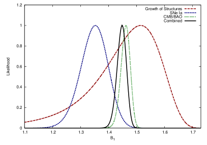
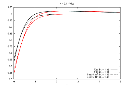
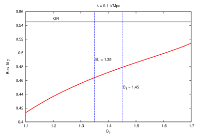
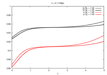
We next look at the modified gravity parameters and . In figure 2 they are plotted with respect to , , and , respectively, with the other two quantities fixed. deviates from the GR value by , while deviates from GR by up to . From the first panel of figure 2 we notice that and lose their dependence on momentarily around . This feature persists to other values of as well. Additionally, we can see from the third panel that and only depend extremely weakly on in the linear subhorizon régime. Future structure experiments like Euclid will be able to constrain and more tightly in a model-independent way because they are effectively scale-independent; in particular, because of scale independence they are expected to be able to measure within 10% Amendola:2013qna , which would bring this minimal model to the cusp of observability.
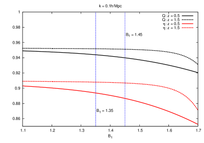
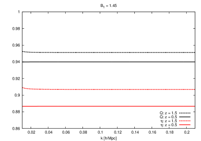
4.2.2 Two-parameter models
At the background level, four models with two nonzero parameters provide good fits to the data: –, –, –, and – Akrami:2012vf . Even though these models all possess a two-dimensional parameter space, only an effectively one-dimensional subspace matches the background data (cf. figures 7 and 8 of Ref. Akrami:2012vf and figure 4 of Ref. Konnig:2013gxa ). We will restrict ourselves to those subspaces by fixing one parameter in terms of another, usually . We do this by identifying the effective present-day dark energy density, , from the Friedmann equation (13):
| (46) |
and plugging that into the quartic equation for (17), evaluated at the present day () and using . This procedure fixes one parameter in terms of the other and . The value of can be determined by fitting to the data, as was done in Ref. Akrami:2012vf . However, for the – models we can also simply take the limit in which only is nonzero, recovering the single-parameter model discussed above; by then using the SNe/CMB/BAO combined best-fit value we find .
A detailed study of the conditions for a viable background was undertaken in Ref. Konnig:2013gxa . There are two results that are particularly relevant for the present study and bear mentioning. First, a viable model requires . Second, the two-parameter models are all (with one exception, which we discuss below) “finite branch” models, in which evolves from 0 at to a finite value at late times, which can be determined from equation 21 by setting at . Consequently, the present-day value of , which is generally simple to calculate, must always be smaller than (or above in a model with an infinite branch). In the – and – models this will rule out certain regions of the parameter space a priori.
All of the two-parameter models except for the infinite-branch – model (so-called “infinite-branch bigravity”) suffer from the early-time instability found in Ref. Konnig:2014xva ; therefore caution should be used when applying the results for any of the other models in this section to real-world data. We emphasize again that our quasistatic approximation is only valid at low redshifts, and that moreover the growth rate should be re-calculated using whatever initial conditions the earlier period ends with. (The predictions for and do not depend on solving any differential equation and therefore apply without change.) Modulo this caveat, we present the quasistatic results for the unstable models as proofs of concept, as examples of how to apply our methods. The infinite-branch bigravity predictions, presented at the end of this section, can be straightforwardly applied to data.
We evaluate all quantities at /Mpc. The modified gravity parameters in all of the two-parameter models we study depend extremely weakly on , as in the -only model.
As we have already mentioned, in these models the two parameters are highly degenerate at the background level. One of the main goals of this section is to see whether observations of LSS have the potential to break this degeneracy.
–:
The – models which fit the background data Akrami:2012vf live in the parameter subspace
| (47) |
with . This line has a slight thickness because we must rely on observations to fit . We can subsequently determine from equation 46.
This model possesses an instability when .191919A similar singular evolution of linear perturbations in a smooth background has been observed in the cosmology of Gauss-Bonnet gravity Kawai:1999pw ; Koivisto:2006xf . This instability is, however, different from the early-time instabilities discussed above, as those instabilities do not arise in the quasistatic limit which we are now taking. This is not entirely unexpected: the term is the coefficient of the quadratic interaction, and so a negative might lead to a tachyonic instability. However, the instability of the – model is somewhat unusual: in the subhorizon limit, and develop poles, but they only diverge during a brief period around a fixed redshift, as shown in the first panel of figure 3, regardless of wavenumber or initial conditions. We can find these poles using the expressions in appendix B. The exact solutions are unwieldy and not enlightening, but there are three notable features. First, as mentioned, the instability only occurs for . (When , these poles occur when is negative, which is not physical.) Second, the instability develops at high redshifts, . The redshift of the latest pole (which can be solved for by taking the limit ) is plotted as a function of in the second panel of figure 3. As a result, measurements of and at would generally not see divergent values. However, such measurements would see the main instabilities at much lower redshifts Konnig:2014xva . Finally, the most recent pole occurs at for (), and approaches as ().
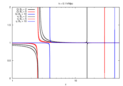
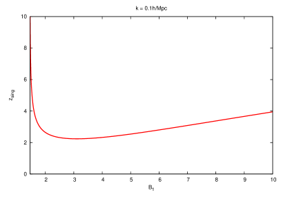
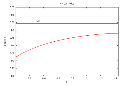
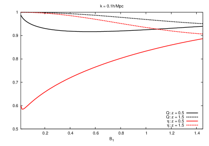
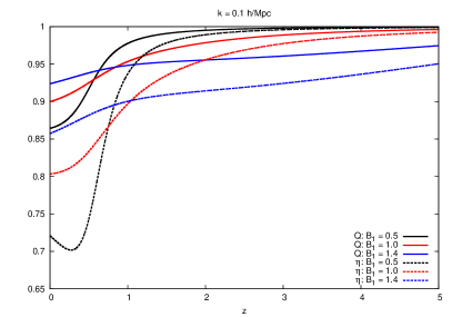
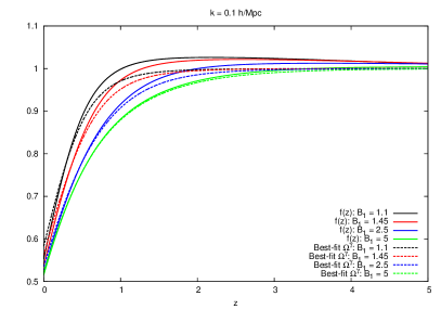
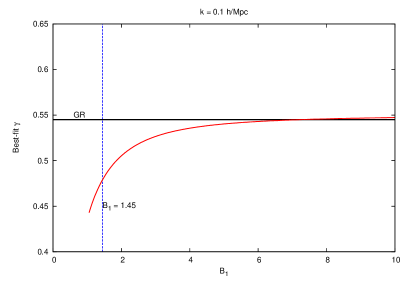
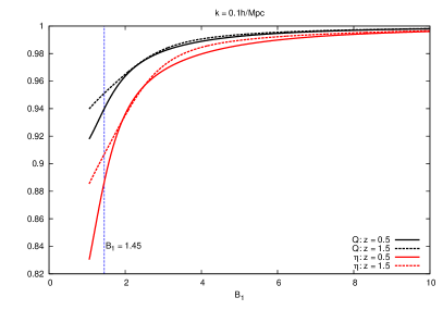
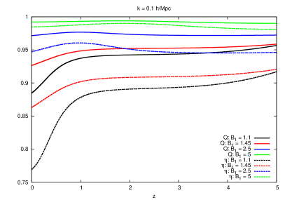
This particular instability is avoided if we restrict ourselves to the range , for which . Some typical results for this region of parameter space are plotted in figure 4. The first panel plots and the best-fit parametrization for selected values of (with given by equation 47), while the second panel shows the best-fit value of as a function of . For smaller values of this parametrization fits well, more so than in the -only model discussed in section 4.2.1 (which is the limit of this model). We find that is always well below the GR value of , especially at low .
In the final two panels we plot and , both in terms of at fixed and in terms of at fixed . In comparison to the -only model (the very right side of the third panel), lowering tends to make these parameters more GR-like, except for evaluated at late times (), which dips as low as . Because these quantities are all -independent in the linear, subhorizon régime, future LSS experiments like Euclid would be able to measure at these redshifts to within about 10% Amendola:2013qna and thus effectively distinguish between CDM and significant portions of the parameter space of the – model, testing the theory and breaking the background-level degeneracy.
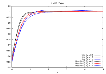
–:
The – models which are consistent with the background data Akrami:2012vf lie along a one-dimensional parameter space (up to a slight thickness) given by
| (48) |
with . There is a subtlety here: the physical branch is constructed in a piecewise fashion, taking the root for and the root otherwise Konnig:2013gxa . We solve for using the initial condition,202020There is also a positive root, but this is not physical. When , that root yields . When , which is only the case for a small range of parameters, then the positive root of is greater than the far-future value and hence is also not physical. derived from equation 17,
| (49) |
As discussed at the beginning of this section, should not be larger than the value of in the far future, . Demanding this, we find a maximum allowed value for ,212121Note, per equation 48, that this is equivalent to simply imposing , which must be true since we have chosen a spatially-flat universe a priori.
| (50) |
For this implies we need to restrict ourselves to . This sort of bound is to be expected: we know that the -only model is a poor fit to the data Akrami:2012vf , so we cannot continue to get viable cosmologies the entire way through the limit of the – model.
We plot the results for the – model in figure 5. These display the tendency, which we will also see in the – model, that large values lead to modified gravity parameters that are closer to GR. For example, can be as low as for the lowest allowed value of , but by it is practically indistinguishable from the GR value, assuming a Euclid-like precision of on Laureijs:2011gra . Again we note that this value of has been obtained assuming , which is not a valid range for observations because of the early-time instability. For lower values of , current growth data (see, e.g., Ref. Macaulay:2013swa ) are not sufficient to significantly constrain the parameter space, but these non-GR values of and should be well within Euclid’s window.
–:
This model comprises the lowest-order term in conjunction with a cosmological constant for the metric, .222222In the singly-coupled version of massive bigravity we are studying, matter loops only contribute to the -metric cosmological constant, . Note that does not contribute directly to the Friedmann equation (13), but only affects the dynamics through its effect on the evolution of .
The – model has two viable solutions for : a finite branch with , and an infinite branch with . The infinite-branch model is the only two-parameter bimetric model which is linearly stable at all times Konnig:2014xva . Therefore this infinite-branch bigravity should be considered the most viable bimetric massive gravity theory to date. In this section we will elucidate its predictions for subhorizon structure formation.
As discussed in the beginning of this section, is the value of in the asymptotic future and can be calculated by setting in equation 21. We will consider the two branches separately.
For a given , is related to by
| (51) |
while is given by
| (52) |
The finite-branch (infinite-branch) condition () imposes
| (53) |
The combination of equations 51 and 53 places a constraint on the allowed range of , as in the – model, which depends on the best-fit value of . The -only model (, ) is on the finite branch, so that on that branch we can use as we did in the other models. This implies for the finite branch. On the infinite branch, SNe observations are best fit by Konnig:2013gxa ; consequently we restrict ourselves to for the infinite branch.
We plot the results for the finite branch in figure 6. Qualitatively, this model predicts subhorizon behavior quite similar to that of the – model, discussed above and plotted in figure 5.
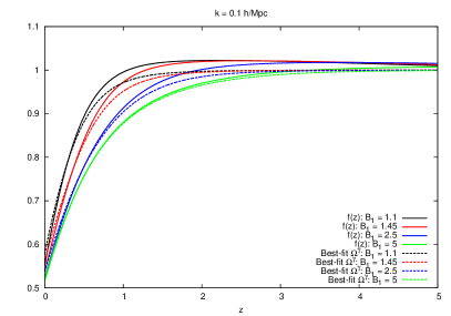
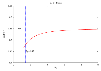
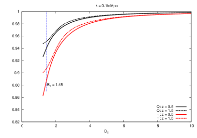
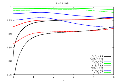
Results for the infinite branch are shown in figure 7. This is the only model we study which does not possess a limit to the minimal -only model, and it predicts significant deviations from GR. deviates from 1 by nearly a factor of 2 at all times and for all allowed values of , providing a clear observable signal of modified gravity.
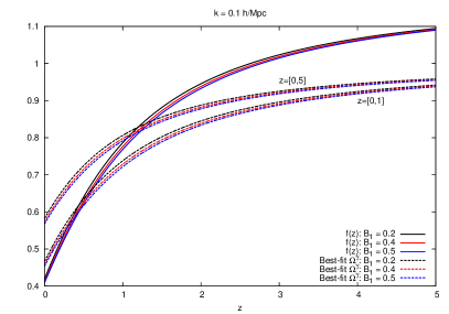
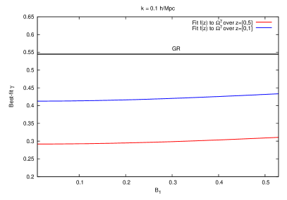
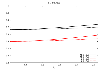
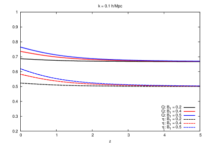
also deviates strongly from the GR value of , and is even lower than the values – which we found in the –only model and in the other two-parameter models. However, it is worth noting that the parametrization is an especially bad fit to in this case, and another parametrization (see, e.g., section 1.8.3 of Ref. Amendola:2012ys ) or even a direct comparison between (multiplied by the growth rate, Amendola:2012ys ; Macaulay:2013swa ) and the data would be more appropriate. We fit to in the redshift range (as in the rest of this paper) and (which is the redshift range of present observations Macaulay:2013swa ) in the first and second panels of figure 7, obtaining significantly different results.
–:
This is a “bouncing” model in the metric: becomes negative in finite time going towards the past, implying that the scale factor collapses to zero and then expands Konnig:2013gxa . This itself may not render the model cosmologically unviable. However, we have solved equation 18 numerically for , and found that generically goes to at finite , which means that at higher redshifts there is not a sensible background cosmology. This problem can be avoided by introducing new physics at those higher redshifts to modify the evolution of , or by increasing enough that the pole in occurs at an unobservably high redshift.232323For , and chosen to give an effective today, the pole occurs at . However, these are nonminimal solutions, and so we do not study the – model.
5 Conclusions
In this paper we have examined the evolution of cosmological perturbations on subhorizon scales, describing linear structure formation during the matter-dominated era, in the massive, ghost-free theory of two interacting metrics. We have studied the most common version of the theory in the literature, in which the matter fields couple to only one of the metrics and couple minimally. We derived the perturbed Einstein equations around FLRW backgrounds and then solved the linearized equations in the subhorizon limit after choosing an appropriate gauge. This gave us the evolution equations for cosmic structure, as well as equations that relate the metric perturbations to the density of matter.
The gauge freedom available to us is the diagonal subgroup of the two diffeomorphism groups for the two metrics; in practice, this means we have a single coordinate chart on which we are free to perform infinitesimal coordinate transformations as in GR, with the same amount of gauge freedom. We chose to work in a Newtonian gauge for the metric, although our results were not sensitive to this choice (for example, we were able to reproduce our results in the gauge of Ref. Konnig:2014dna , ). In the subhorizon limit, we found that the perturbations were described by a system of six algebraic equations for five variables, and obtained a consistent solution. This solution relates each of the metric perturbations appearing in the subhorizon Einstein equations to the matter density. This allowed us to derive a modified evolution equation for the density contrast, which differs from its GR counterpart by a varying effective Newton’s constant, as well as algebraic expressions for the anisotropic stress, , and the parameter measuring modifications to Newton’s constant in the Poisson equation, , purely in terms of background quantities. We then solved for the background numerically to obtain these parameters, and finally integrated the structure growth equation to derive the growth rate, and its best-fit parametrization, .
We have studied every subset of the theory which is a) viable at the background level, and b) contains one or two free parameters, while excluding the -metric cosmological constant as we are interested in self-accelerating theories that differ from CDM. Among the single-parameter models, only the case with the lowest-order interaction term, , is in agreement with the background data. We have found that it predicts modified gravity parameters that differ significantly from GR: – (in agreement with Ref. Konnig:2014dna ), –, and –. For reference, the CDM predictions are and . Future large-scale structure experiments such as Euclid Laureijs:2011gra ; Amendola:2012ys will easily be able to distinguish this simple model from GR. As emphasized in Refs. Akrami:2012vf ; Akrami:2013pna ; Konnig:2013gxa , this “minimal” bigravity model is especially appealing because it possesses late-time acceleration and fits the background data well with the same number of free parameters as CDM. It suffers from an early-time instability Konnig:2014xva ; however, if this can be overcome, or if observations are restricted to late times (), our results demonstrate that by going to the level of linear perturbations, this theory can be probed in the near future by multiple observables which deviate significantly from general relativity.
We additionally examined the four two-parameter models that are viable in the background, all of which keep while turning on a second, higher-order interaction term. Two models, in which either the cubic interaction or the -metric cosmological constant is nonzero (the latter specifically in the “finite branch,” which reduces to the minimal model in the limit), have similar behavior. They predict GR-like values for all three modified gravity parameters in the limit where is large, becoming indistinguishable from CDM (given a Euclid-like experiment) for . These reduce to the predictions of the minimal model in the limit (the best-fit value for in the minimal model). For lower values of (corresponding to positive or ) these models predict even more dramatic deviations from GR: can dip to , and at recent times can be as low as . Euclid is expected to measure these parameters to within about and , respectively Laureijs:2011gra ; Amendola:2012ys ; Amendola:2013qna , and therefore has the potential to break the degeneracies between and or and which is present at the level of background observations.
The – model has an instability when , the coefficient of the quadratic term, is negative. This instability does not necessarily rule out the theory, but it might signal the breakdown of linear perturbation theory, in which case nonlinear studies are required in order to understand the formation of structures. This is different from the early-time instability which is present in all but the infinite-branch – model and does not show up in the subhorizon, quasistatic régime. It is possible that these perturbations at some point become GR-like due to the Vainshtein mechanism. Moreover, because the instability occurs at a characteristic redshift (which depends on the parameters), there may be an observable excess of cosmic structure around that redshift. We leave this to future work.
The parameter range of the – model over which linear, subhorizon perturbations are stable, (corresponding to ), is quite small; near the large end the predictions recover those of the minimal -only model, while at the small end the perturbations can differ quite significantly from GR, with as low as and as low as 0.6. However, the exact limit of this theory is already ruled out by background observations Akrami:2012vf , so one should take care when comparing the model to observations in the very low region of this parameter space.
Finally, we examined the “infinite branch” of the – model, in which the ratio of the metric scale factor to the metric scale factor starts at infinity and monotonically decreases to a finite value. In the rest of the models we study, the ratio of the two scale factors starts at zero and then increases; consequently in the limit, this theory reduces to pure CDM, rather than to the -only model. The predictions of the infinite-branch – theory deviate strongly from GR. The model predicts a growth rate which is not well-parametrized by a fit, but has best-fit values of on the low side (–, depending on the fitting range). The anisotropic stress is almost always below and can even be as low as , a factor of two away from the GR prediction. Across its entire parameter space, this model has the most significantly non-GR values of any we study, and is almost certainly the bigravity model which is viable at the background level that structure observations will be able to rule out first.
Significantly, this infinite-branch – model, or infinite-branch bigravity, is stable at all times Konnig:2014xva . As the only two-parameter massive bigravity model which both self-accelerates and is always linearly stable around cosmological backgrounds, it is a prime target for observational study.
To summarize, the new ghost-free theory of massive bigravity, in which the graviton is given mass and coupled to a new, metric-like massless spin-2 field, predicts structure formation that deviates significantly from the predictions of general relativity, even while matching the cosmic expansion history as well as CDM does. These deviations are on the cusp of observability given the impending wave of large-scale structure experiments such as Euclid Laureijs:2011gra ; Amendola:2012ys . This leaves the exciting prospect of observations in the near future ruling out either the simplest theory of a massless graviton or the simplest theory of a massive one. It is worth noting, however, that by making the free parameters large enough, or perhaps by adding a third or fourth interaction term, these constraints can still in principle be evaded. The question remains how to address these remaining corners of the theory, and further — in the event that large-scale structure experiments observe deviations from GR — how to distinguish between certain regions of the bigravity parameter space which have similar predictions. Since the theory is an IR modification of gravity, i.e., its new effects are most significant near the horizon, we expect new observational signatures to exist at superhorizon scales. This may affect the inflationary primordial power spectrum at large scales and/or leave detectable effects on the CMB, such as in the integrated Sachs-Wolfe effect. We leave the investigation of such possible superhorizon signatures, as well as a study of the nonlinear structures in this framework, for future work.
Acknowledgements.
We thank Phil Bull, Jonas Enander, Fawad Hassan, and Edvard Mörtsell for helpful discussions. We are especially grateful to Luca Amendola and Frank Könnig for clarifying discussions during the preparation of an early draft of this paper. A.R.S. is supported by the David Gledhill Research Studentship, Sidney Sussex College, University of Cambridge; and by the Isaac Newton Fund and Studentships, University of Cambridge. Y.A. is supported by the European Research Council (ERC) Starting Grant StG2010-257080. We acknowledge the use of resources from the Norwegian national super-computing facilities, NOTUR.Appendix A Full perturbation equations
Defining the perturbed metrics as242424By leaving the lapse in the metric general, we retain the freedom to later work in cosmic or conformal time. There is a further practical benefit: since this choice makes the symmetry between the two metrics manifest, and the action is symmetric between and as described in section 2, this means the field equations can easily be derived from the equations by judicious use of ctrl-f.
| (54) | ||||
| (55) |
the linearized Einstein equations for the metric are
-
•
:
(56) -
•
:
(57) -
•
:
(58) (59) -
•
Off-diagonal :
(60)
where is the usual -metric Hubble parameter (in cosmic or conformal time, depending on ), in the spatial Einstein equation refers to derivatives w.r.t. the other two Cartesian coordinates, i.e., where the indices are not summed over, and
| (61) | ||||
| (62) | ||||
| (63) | ||||
| (64) | ||||
| (65) | ||||
| (66) | ||||
| (67) |
The linearized Einstein equations for the metric are
-
•
:
(68) -
•
:
(69) -
•
:
(70) (71) -
•
Off-diagonal :
(72)
where is the -metric Hubble parameter.
It is worth mentioning that the equation, (58), is identically zero in GR after taking into account the , off-diagonal , and fluid conservation equations and hence gives no information; in massive (bi)gravity, however, it is crucial, and is manifestly only important when . In a gauge with it has the simple form
| (73) |
This should be compared to equation 37. Moreover, performing the same steps on the equation, we arrive again at equation 73. Hence both equations carry the same information.
Since these equations are arrived at by a fairly lengthy calculation, for the convenience of future generations of bigravitists we now present some helpful intermediate relations. The metric determinants to linear order are
| (74) | ||||
| (75) |
The matrix is defined in terms of the two metrics as
| (76) |
Its background value is simply
| (77) |
Using this we can solve equation 76 to first order in perturbations to find
| (78) |
The trace of this is
| (79) |
Similarly we can solve for the matrix , although we do not write its components here as they can be found by simply substituting with and vice versa.252525It may also be calculated explicitly or by using the fact that is simply the matrix inverse of , which can be easily inverted to first order.
We now need the matrices and and their traces in order to compute the matrices appearing in the mass terms of the Einstein equations. For we find
| (80) |
with trace
| (81) |
is given by
| (82) |
with trace
| (83) |
and can be determined trivially from these.
With these we can determine the functions and . Two helpful intermediate results are
| (84) | ||||
| (85) |
To obtain those intermediate results and the and components of the matrices, it saves a lot of algebra to write the traces, components, and components of the various matrices in terms of
| (86) | |||||||
Finally, the matrices defined in equation 6 are given by:
-
•
:
(87) -
•
:
(88) -
•
:
(89) -
•
:
(90)
Plugging these matrices into the field equations 4 and 5, we obtain the full perturbation equations presented at the beginning of this appendix.
Appendix B Explicit solutions for the modified gravity parameters
As discussed in section 4, the modified gravity parameters and have the Horndeski form,
| (91) | ||||
| (92) |
while the growth of structures can be written in these terms as
| (93) |
Hence the five coefficients allow us to determine all three modified gravity parameters we consider in this paper. They are given explicitly by
| (94) | ||||
| (95) | ||||
| (96) | ||||
| (97) | ||||
| (98) | ||||
| (99) | ||||
| (100) |
While this notation is inspired by Refs. Amendola:2012ky ; Amendola:2013qna , we have defined differently.
References
- (1) M. Fierz and W. Pauli, On relativistic wave equations for particles of arbitrary spin in an electromagnetic field, Proceedings of the Royal Society of London. Series A, Mathematical and Physical Sciences (1939) 211–232.
- (2) C. Isham, A. Salam, and J. Strathdee, F-dominance of gravity, Phys.Rev. D3 (1971) 867–873.
- (3) S. Deser and D. G. Boulware, Can gravitation have a finite range?, Phys. Rev. D6 (1972) 3368–3382.
- (4) C. de Rham and G. Gabadadze, Generalization of the Fierz-Pauli Action, Phys.Rev. D82 (2010) 044020, [arXiv:1007.0443].
- (5) C. de Rham, G. Gabadadze, and A. J. Tolley, Resummation of Massive Gravity, Phys.Rev.Lett. 106 (2011) 231101, [arXiv:1011.1232].
- (6) C. de Rham, G. Gabadadze, and A. J. Tolley, Ghost free Massive Gravity in the Stúckelberg language, Phys.Lett. B711 (2012) 190–195, [arXiv:1107.3820].
- (7) C. de Rham, G. Gabadadze, and A. J. Tolley, Helicity Decomposition of Ghost-free Massive Gravity, JHEP 1111 (2011) 093, [arXiv:1108.4521].
- (8) S. F. Hassan and R. A. Rosen, On Non-Linear Actions for Massive Gravity, JHEP 07 (2011) 009, [arXiv:1103.6055].
- (9) S. Hassan and R. A. Rosen, Resolving the Ghost Problem in non-Linear Massive Gravity, Phys.Rev.Lett. 108 (2012) 041101, [arXiv:1106.3344].
- (10) A. Golovnev, On the Hamiltonian analysis of non-linear massive gravity, Phys.Lett. B707 (2012) 404–408, [arXiv:1112.2134].
- (11) S. Hassan and R. A. Rosen, Confirmation of the Secondary Constraint and Absence of Ghost in Massive Gravity and Bimetric Gravity, JHEP 1204 (2012) 123, [arXiv:1111.2070].
- (12) S. Hassan, A. Schmidt-May, and M. von Strauss, Proof of Consistency of Nonlinear Massive Gravity in the Stúckelberg Formulation, Phys.Lett. B715 (2012) 335–339, [arXiv:1203.5283].
- (13) J. Kluson, Non-Linear Massive Gravity with Additional Primary Constraint and Absence of Ghosts, Phys.Rev. D86 (2012) 044024, [arXiv:1204.2957].
- (14) K. Nomura and J. Soda, When is Multimetric Gravity Ghost-free?, Phys.Rev. D86 (2012) 084052, [arXiv:1207.3637].
- (15) A. Golovnev, ADM analysis and massive gravity, arXiv:1302.0687.
- (16) J. Kluson, Is Bimetric Gravity Really Ghost Free?, arXiv:1301.3296.
- (17) A. Golovnev, On non-perturbative analysis of massive and bimetric gravity, arXiv:1401.6343.
- (18) C. de Rham, Massive Gravity, arXiv:1401.4173.
- (19) C. de Rham, A. Matas, and A. J. Tolley, New Kinetic Interactions for Massive Gravity?, arXiv:1311.6485.
- (20) X. Gao, On derivative interactions for a spin-2 field at cubic order, arXiv:1403.6781.
- (21) S. F. Hassan, R. A. Rosen, and A. Schmidt-May, Ghost-free Massive Gravity with a General Reference Metric, JHEP 02 (2012) 026, [arXiv:1109.3230].
- (22) S. F. Hassan and R. A. Rosen, Bimetric Gravity from Ghost-free Massive Gravity, JHEP 02 (2012) 126, [arXiv:1109.3515].
- (23) S. Deser, K. Izumi, Y. Ong, and A. Waldron, Superluminal Propagation and Acausality of Nonlinear Massive Gravity, arXiv:1312.1115.
- (24) S. Deser and A. Waldron, Non-Einstein source effects in massive gravity, Phys.Rev. D89 (2014) 027503, [arXiv:1310.2675].
- (25) Y. Akrami, T. S. Koivisto, D. F. Mota, and M. Sandstad, Bimetric gravity doubly coupled to matter: theory and cosmological implications, JCAP 1310 (2013) 046, [arXiv:1306.0004].
- (26) N. Tamanini, E. N. Saridakis, and T. S. Koivisto, The Cosmology of Interacting Spin-2 Fields, arXiv:1307.5984.
- (27) Y. Akrami, T. S. Koivisto, and A. R. Solomon, The nature of spacetime in bigravity: two metrics or none?, arXiv:1404.0006.
- (28) N. Khosravi, N. Rahmanpour, H. R. Sepangi, and S. Shahidi, Multi-Metric Gravity via Massive Gravity, Phys.Rev. D85 (2012) 024049, [arXiv:1111.5346].
- (29) V. Baccetti, P. Martin-Moruno, and M. Visser, Massive gravity from bimetric gravity, Class.Quant.Grav. 30 (2013) 015004, [arXiv:1205.2158].
- (30) V. Baccetti, P. Martin-Moruno, and M. Visser, Null Energy Condition violations in bimetric gravity, JHEP 1208 (2012) 148, [arXiv:1206.3814].
- (31) S. Capozziello and P. Martin-Moruno, Bounces, turnarounds and singularities in bimetric gravity, Phys.Lett. B719 (2013) 14–17, [arXiv:1211.0214].
- (32) D. Comelli, M. Crisostomi, and L. Pilo, FRW Cosmological Perturbations in Massive Bigravity, arXiv:1403.5679.
- (33) A. De Felice, A. E. Gümrükçüoğlu, S. Mukohyama, N. Tanahashi, and T. Tanaka, Viable cosmology in bimetric theory, arXiv:1404.0008.
- (34) Y. Yamashita, A. De Felice, and T. Tanaka, Appearance of Boulware-Deser ghost in bigravity with doubly coupled matter, arXiv:1408.0487.
- (35) C. de Rham, L. Heisenberg, and R. H. Ribeiro, On couplings to matter in massive (bi-)gravity, arXiv:1408.1678.
- (36) J. Noller and S. Melville, The coupling to matter in Massive, Bi- and Multi-Gravity, arXiv:1408.5131.
- (37) A. Schmidt-May, Mass eigenstates in bimetric theory with ghost-free matter coupling, arXiv:1409.3146.
- (38) J. Enander, A. R. Solomon, Y. Akrami, and E. Mortsell, Cosmic expansion histories in doubly-coupled, ghost-free massive bigravity, arXiv:1409.2860.
- (39) A. E. Gümrükçüoğlu, L. Heisenberg, and S. Mukohyama, Cosmological perturbations in massive gravity with doubly coupled matter, arXiv:1409.7260.
- (40) A. R. Solomon, J. Enander, Y. Akrami, T. S. Koivisto, F. Könnig, et al., Does massive gravity have viable cosmologies?, arXiv:1409.8300.
- (41) C. de Rham, L. Heisenberg, and R. H. Ribeiro, Ghosts & Matter Couplings in Massive (bi-&multi-)Gravity, arXiv:1409.3834.
- (42) S. Hassan, M. Kocic, and A. Schmidt-May, Absence of ghost in a new bimetric-matter coupling, arXiv:1409.1909.
- (43) S. Nojiri and S. D. Odintsov, Ghost-free bigravity and accelerating cosmology, Phys.Lett. B716 (2012) 377–383, [arXiv:1207.5106].
- (44) S. Nojiri, S. D. Odintsov, and N. Shirai, Variety of cosmic acceleration models from massive bigravity, arXiv:1212.2079.
- (45) M. F. Paulos and A. J. Tolley, Massive Gravity Theories and limits of Ghost-free Bigravity models, JHEP 1209 (2012) 002, [arXiv:1203.4268].
- (46) Y.-F. Cai, C. Gao, and E. N. Saridakis, Bounce and cyclic cosmology in extended nonlinear massive gravity, JCAP 1210 (2012) 048, [arXiv:1207.3786].
- (47) Q.-G. Huang, Y.-S. Piao, and S.-Y. Zhou, Mass-Varying Massive Gravity, Phys.Rev. D86 (2012) 124014, [arXiv:1206.5678].
- (48) D.-J. Wu, Y.-S. Piao, and Y.-F. Cai, Dynamical analysis of the cosmology of mass-varying massive gravity, Phys.Lett. B721 (2013) 7–12, [arXiv:1301.4326].
- (49) G. Leon, J. Saavedra, and E. N. Saridakis, Cosmological behavior in extended nonlinear massive gravity, arXiv:1301.7419.
- (50) S. Hossenfelder, A Bi-Metric Theory with Exchange Symmetry, Phys.Rev. D78 (2008) 044015, [arXiv:0807.2838].
- (51) L. Amendola, K. Enqvist, and T. Koivisto, Unifying Einstein and Palatini gravities, Phys.Rev. D83 (2011) 044016, [arXiv:1010.4776].
- (52) J. Beltran Jimenez, A. Golovnev, M. Karciauskas, and T. S. Koivisto, The Bimetric variational principle for General Relativity, Phys.Rev. D86 (2012) 084024, [arXiv:1201.4018].
- (53) T. S. Koivisto, On new variational principles as alternatives to the Palatini method, Phys.Rev. D83 (2011) 101501, [arXiv:1103.2743].
- (54) N. Tamanini, Variational approach to gravitational theories with two independent connections, Phys.Rev. D86 (2012) 024004, [arXiv:1205.2511].
- (55) N. Khosravi, Geometric Massive Gravity in Multi-Connection Framework, Phys.Rev. D89 (2014) 024004, [arXiv:1309.2291].
- (56) M. Jaccard, M. Maggiore, and E. Mitsou, Nonlocal theory of massive gravity, Phys.Rev. D88 (2013), no. 4 044033, [arXiv:1305.3034].
- (57) M. Maggiore, Phantom dark energy from non-local infrared modifications of General Relativity, Phys.Rev. D89 (2014) 043008, [arXiv:1307.3898].
- (58) S. Nesseris and S. Tsujikawa, Cosmological perturbations and observational constraints on non-local massive gravity, arXiv:1402.4613.
- (59) M. Maggiore and M. Mancarella, Non-local gravity and dark energy, arXiv:1402.0448.
- (60) L. Modesto and S. Tsujikawa, Non-local massive gravity, arXiv:1307.6968.
- (61) S. Hassan, A. Schmidt-May, and M. von Strauss, Higher Derivative Gravity and Conformal Gravity From Bimetric and Partially Massless Bimetric Theory, arXiv:1303.6940.
- (62) G. Cusin, J. Fumagalli, and M. Maggiore, Non-local formulation of ghost-free bigravity theory, arXiv:1407.5580.
- (63) EUCLID Collaboration, R. Laureijs et al., Euclid Definition Study Report, arXiv:1110.3193.
- (64) Euclid Theory Working Group Collaboration, L. Amendola et al., Cosmology and fundamental physics with the Euclid satellite, Living Rev.Rel. 16 (2013) 6, [arXiv:1206.1225].
- (65) M. S. Volkov, Cosmological solutions with massive gravitons in the bigravity theory, JHEP 1201 (2012) 035, [arXiv:1110.6153].
- (66) D. Comelli, M. Crisostomi, F. Nesti, and L. Pilo, FRW Cosmology in Ghost Free Massive Gravity, JHEP 1203 (2012) 067, [arXiv:1111.1983].
- (67) M. von Strauss, A. Schmidt-May, J. Enander, E. Mortsell, and S. Hassan, Cosmological Solutions in Bimetric Gravity and their Observational Tests, JCAP 1203 (2012) 042, [arXiv:1111.1655].
- (68) M. S. Volkov, Cosmological solutions with massive gravitons in the bigravity theory, JHEP 1201 (2012) 035, [arXiv:1110.6153].
- (69) M. S. Volkov, Exact self-accelerating cosmologies in the ghost-free massive gravity – the detailed derivation, Phys.Rev. D86 (2012) 104022, [arXiv:1207.3723].
- (70) M. Berg, I. Buchberger, J. Enander, E. Mortsell, and S. Sjors, Growth Histories in Bimetric Massive Gravity, JCAP 1212 (2012) 021, [arXiv:1206.3496].
- (71) Y. Akrami, T. S. Koivisto, and M. Sandstad, Accelerated expansion from ghost-free bigravity: a statistical analysis with improved generality, JHEP 1303 (2013) 099, [arXiv:1209.0457].
- (72) Y. Akrami, T. S. Koivisto, and M. Sandstad, Cosmological constraints on ghost-free bigravity: background dynamics and late-time acceleration, arXiv:1302.5268.
- (73) J. Enander and E. Mörtsell, Strong lensing constraints on bimetric massive gravity, JHEP 1310 (2013) 031, [arXiv:1306.1086].
- (74) F. Koennig, A. Patil, and L. Amendola, Viable cosmological solutions in massive bimetric gravity, JCAP 1403 (2014) 029, [arXiv:1312.3208].
- (75) F. Könnig and L. Amendola, A minimal bimetric gravity model that fits cosmological observations, arXiv:1402.1988.
- (76) D. Comelli, M. Crisostomi, and L. Pilo, Perturbations in Massive Gravity Cosmology, JHEP 1206 (2012) 085, [arXiv:1202.1986].
- (77) F. Könnig, Y. Akrami, L. Amendola, M. Motta, and A. R. Solomon, Stable and unstable cosmological models in bimetric massive gravity, arXiv:1407.4331.
- (78) S. Hassan, A. Schmidt-May, and M. von Strauss, On Consistent Theories of Massive Spin-2 Fields Coupled to Gravity, arXiv:1208.1515.
- (79) G. W. Horndeski, Second-order scalar-tensor field equations in a four-dimensional space, Int.J.Theor.Phys. 10 (1974) 363–384.
- (80) C. Deffayet, X. Gao, D. Steer, and G. Zahariade, From k-essence to generalised Galileons, Phys.Rev. D84 (2011) 064039, [arXiv:1103.3260].
- (81) T. Jacobson, Einstein-aether gravity: A Status report, PoS QG-PH (2007) 020, [arXiv:0801.1547].
- (82) A. R. Solomon and J. D. Barrow, Inflationary Instabilities of Einstein-Aether Cosmology, Phys.Rev. D89 (2014) 024001, [arXiv:1309.4778].
- (83) C. de Rham, L. Heisenberg, and R. H. Ribeiro, Quantum Corrections in Massive Gravity, Phys.Rev. D88 (2013) 084058, [arXiv:1307.7169].
- (84) T.-C. Chang, U.-L. Pen, J. B. Peterson, and P. McDonald, Baryon Acoustic Oscillation Intensity Mapping as a Test of Dark Energy, Phys.Rev.Lett. 100 (2008) 091303, [arXiv:0709.3672].
- (85) P. Bull, P. G. Ferreira, P. Patel, and M. G. Santos, Late-time cosmology with 21cm intensity mapping experiments, arXiv:1405.1452.
- (86) E. Majerotto, L. Guzzo, L. Samushia, W. J. Percival, Y. Wang, et al., Probing deviations from General Relativity with the Euclid spectroscopic survey, Mon.Not.Roy.Astron.Soc. 424 (2012) 1392–1408, [arXiv:1205.6215].
- (87) M. Fasiello and A. J. Tolley, Cosmological Stability Bound in Massive Gravity and Bigravity, JCAP 1312 (2013) 002, [arXiv:1308.1647].
- (88) A. De Felice, T. Kobayashi, and S. Tsujikawa, Effective gravitational couplings for cosmological perturbations in the most general scalar-tensor theories with second-order field equations, Phys.Lett. B706 (2011) 123–133, [arXiv:1108.4242].
- (89) L. Amendola, M. Kunz, M. Motta, I. D. Saltas, and I. Sawicki, Observables and unobservables in dark energy cosmologies, Phys.Rev. D87 (2013) 023501, [arXiv:1210.0439].
- (90) L. Amendola, S. Fogli, A. Guarnizo, M. Kunz, and A. Vollmer, Model-independent constraints on the cosmological anisotropic stress, Phys.Rev. D89 (2014) 063538, [arXiv:1311.4765].
- (91) N. Suzuki, D. Rubin, C. Lidman, G. Aldering, R. Amanullah, et al., The Hubble Space Telescope Cluster Supernova Survey: V. Improving the Dark Energy Constraints Above and Building an Early-Type-Hosted Supernova Sample, Astrophys.J. 746 (2012) 85, [arXiv:1105.3470].
- (92) WMAP Collaboration, E. Komatsu et al., Seven-Year Wilkinson Microwave Anisotropy Probe (WMAP) Observations: Cosmological Interpretation, Astrophys.J.Suppl. 192 (2011) 18, [arXiv:1001.4538].
- (93) F. Beutler, C. Blake, M. Colless, D. H. Jones, L. Staveley-Smith, et al., The 6dF Galaxy Survey: Baryon Acoustic Oscillations and the Local Hubble Constant, Mon.Not.Roy.Astron.Soc. 416 (2011) 3017–3032, [arXiv:1106.3366].
- (94) SDSS Collaboration, W. J. Percival et al., Baryon Acoustic Oscillations in the Sloan Digital Sky Survey Data Release 7 Galaxy Sample, Mon.Not.Roy.Astron.Soc. 401 (2010) 2148–2168, [arXiv:0907.1660].
- (95) C. Blake, E. Kazin, F. Beutler, T. Davis, D. Parkinson, et al., The WiggleZ Dark Energy Survey: mapping the distance-redshift relation with baryon acoustic oscillations, Mon.Not.Roy.Astron.Soc. 418 (2011) 1707–1724, [arXiv:1108.2635].
- (96) E. Macaulay, I. K. Wehus, and H. K. Eriksen, A Lower Growth Rate from Recent Redshift Space Distortions than Expected from Planck, arXiv:1303.6583.
- (97) F. Beutler, C. Blake, M. Colless, D. H. Jones, L. Staveley-Smith, et al., The 6dF Galaxy Survey: measurement of the growth rate and , Mon.Not.Roy.Astron.Soc. 423 (2012) 3430–3444, [arXiv:1204.4725].
- (98) L. Samushia, W. J. Percival, and A. Raccanelli, Interpreting large-scale redshift-space distortion measurements, Mon.Not.Roy.Astron.Soc. 420 (2012) 2102–2119, [arXiv:1102.1014].
- (99) R. Tojeiro, W. Percival, J. Brinkmann, J. Brownstein, D. Eisenstein, et al., The clustering of galaxies in the SDSS-III Baryon Oscillation Spectroscopic Survey: measuring structure growth using passive galaxies, arXiv:1203.6565.
- (100) C. Blake, S. Brough, M. Colless, C. Contreras, W. Couch, et al., The WiggleZ Dark Energy Survey: Joint measurements of the expansion and growth history at , Mon.Not.Roy.Astron.Soc. 425 (2012) 405–414, [arXiv:1204.3674].
- (101) S. de la Torre, L. Guzzo, J. Peacock, E. Branchini, A. Iovino, et al., The VIMOS Public Extragalactic Redshift Survey (VIPERS). Galaxy clustering and redshift-space distortions at in the first data release, arXiv:1303.2622.
- (102) S. Kawai and J. Soda, Evolution of fluctuations during graceful exit in string cosmology, Phys.Lett. B460 (1999) 41–46, [gr-qc/9903017].
- (103) T. Koivisto and D. F. Mota, Cosmology and Astrophysical Constraints of Gauss-Bonnet Dark Energy, Phys.Lett. B644 (2007) 104–108, [astro-ph/0606078].