Deriving model-based T_e-consistent chemical abundances in ionised gaseous nebulae

Abstract

The derivation of abundances in gaseous nebulae ionised by massive stars using optical collisionally excited emission lines is studied in this work comparing the direct or $T_{e}$ method with updated grids of photoionisation models covering a wide range of input conditions of O/H and N/O abundances and ionisation parameter. The abundances in a large sample of compiled objects with at least one auroral line are re-derived and later compared with the $\chi^{2}$ weighted-mean abundances from the models. The agreement between the abundances using the two methods both for O/H and N/O is excellent with no additional assumptions about the geometry or physics governing the H ii regions. Although very inaccurate model-based O/H are obtained when no auroral lines are considered, this can be overcome assuming empirical laws between O/H, log $U$, and N/O to constrain the considered models. In this way, for 12+log(O/H) $>$ 8.0, a precision better than 0.1dex consistent with the direct method is attained. For very low-$Z$, models give higher O/H values and a high dispersion, possibly owing to the contamination of the low-excitation emission-lines. However, in this regime, the auroral lines are usually well-detected. The use of this procedure, in a publicly available script, hii-chi-mistry, leads to the derivation of abundances in faint/high redshift objects consistent with the direct method based on CELs.

1 Introduction

Metalllicity ($Z$) is one of the most relevant quantities to correctly characterize the nature of astrophysical objects, including from planets and stars up to galaxies. For instance, in the early Universe an accurate determination of $Z$ as a function of the cosmic age and other properties of galaxies renders very valuable information about the evolution of the Universe itself. At these distances, the collisionally excited lines (CELs) emitted by different chemical species in the gas ionised by massive episodes of star-formation is almost the unique way to access to this information. Owing to the strong dependence of CELs on electron temperature ($T_{e}$), the method used to derive chemical abundances using these lines relies necessarily on the previous determination of $T_{e}$, using the so-called direct method. In the case of the optical spectral range, the temperature can be estimated using specific auroral-to-nebular emission line ratios, such as [O iii] I(5007Å)/I(4363Å).

However, as auroral emission lines are much fainter than nebular strong lines, a direct estimation of $T_{e}$ is difficult in faint/distant objects or in the high-$Z$ regime, where the cooling is more efficient and the temperature is then lower. In this case, strong-line methods based only on the nebular CELs are used. In order to provide a $Z$ absolute scale consistent with the direct method, some authors have provided empirical calibration of these strong-line methods (e.g. Pilyugin & Thuan 2005; Pettini & Pagel 2004; Pérez-Montero & Díaz 2005). This methodology has the advantage that is well correlated with direct observations but, on the contrary, can lead to biases in the scale towards the objects with a good measurement of the auroral lines (Stasińska, 2010). In this case, a calibration of the strong-line methods based on models ensure that all conditions can be envisaged. The main problem is that many of the most widely used calibrations based on models (e.g. McGaugh 1991; Charlot & Longhetti 2001; Kewley & Dopita 2002) give systematic overabundances in relation with the direct method. These differences can be as high as 0.7dex depending on the models and the $Z$ regime (see for a discussion on this Kewley & Ellison 2008).

In the same sense, the direct method based on CELs has been widely questioned based on the controversial results coming from other observational techniques in the same objects where the CELs have been detected. For instance, the use of recombination lines (RLs) emitted by heavy elements, which are around 10⁴ times fainter than CELs, but they do not depend on temperature, lead to abundances 0.1-0.3dex higher both in Giant H ii regions (e.g. Esteban et al. 2009 and references therein) and even higher in planetary nebulae (e.g. Liu 2010 and references therein). This discrepancy is not probably due to the use of old sets of atomic data for the RLs (Fang & Liu, 2013). On the other hand, the abundances derived from OB supergiants give controversial results about the value of the discrepancy with abundances from CELs. Some works point to little difference with CELs (e.g. NGC300, Bresolin et al. 2009), and while some others point to values quite similar to those obtained from RLs (e.g. Simón-Díaz & Stasińska 2011; Firnstein & Przybilla 2012).

We can find different explanations in the literature to account for these differences, including the presence of fluctuations of temperature (Peimbert, 1967), which makes the integrated $T_{e}$ derived from CELs ratios to be systematically overestimated and, hence, lead to an underestimation of the metallicity. Other possible cause is found in the existence of chemical inhomogeneities (Tsamis & Péquignot, 2005; Dors et al., 2013) or, more recently, in a possible asymmetric energy distribution for the free electrons in the ionised gas (the $k$ distribution, Nicholls et al. 2012).

The existence of these discrepancies has been used as an argument to justify the disagreement found between the calibrations of strong-line methods based on models and based on observations of CELs. Nevertheless, the physical causes thought to be responsible for these discrepancies are not included in the models and even some tailor-made models for low-$Z$ objects, in which [O iii] 4363 Å is visible give chemical abundances in good agreement with those derived from the direct method (e.g. Pérez-Montero & Díaz 2007; Pérez-Montero et al. 2010; Dors et al. 2011).

This work studies if photoionisation models can lead to a determination of chemical abundances consistent with the calculations obtained using the direct method both with and without measuring auroral emission lines. To this aim, Section 2 presents a sample of ionised gaseous nebulae with good measurements of their CELs, including at least one auroral emission line, and their O/H and N/O are re-calculated using expressions consistent with the code pyneb and updated sets of atomic data. Section 3 describes a large grid of photoionisation models covering a wide range of properties in O/H, N/O, and log $U$. and a procedure based on a $\chi^{2}$-weighted mean is presented. Section 4 analyses the consistency of the abundances obtained using the two methods, and discusses what happens when the number of available emission lines is limited in the models. Finally, Section 5 summarises the results and presents the conclusions.

2 Data description

This study uses the compilation of emission-line fluxes in ionised gaseous nebulae carried out by Marino et al. (2013) to provide a data sample that can be later compared with the results obtained from models. This sample comprises 550 objects collected from the literature with the measurement with good S/N of at least one auroral emission-line and hence an empirical estimate of $T_{e}$. It is an heterogeneous sample of pure star-forming low-density (i.e. $n_{e}<$ 1000 cm^-3) emission-line objects in the Local Universe including H ii galaxies, giant extragalactic H ii regions, and diffuse H ii regions in our own Galaxy and in the Magellanic Clouds. This sample is the largest available so far with $T_{e}$ and covers a wide range in O/H from 12+log(O/H) = 7.1 (SBS0335-052) up to 9.1 (H13 in NGC628)] and N/O [from log(N/O) = -1.95 (NGC5253) up to -0.14 (NGC5236)]. The emission-lines measured by means of integrated spectroscopy of the brightest H ii regions were consistently reddening corrected by Marino et al. (2013) and later used to calculate chemical abundances according with the direct method.

In this sample, an empirical estimate of the [O iii] $T_{e}$ by means of the I(5007)/I(4363) can be performed in 497 objects. In 76 objects, 17 of them also belong to the sample with t[O iii], the [N ii]$T_{e}$ can be derived empirically using the I(6584)/I(5755). The leftover 37 objects have an estimate of $T_{e}$ of [S iii] by means of the ratio I(9532)/I(6312). Both t[N ii] and t[S iii] can be derived more easily than t[O iii] in high-$Z$ objects as the emissivity of the corresponding emission-lines depends less on $T_{e}$ (Bresolin, 2007).

2.1 Derivation of physical properties and chemical abundances

For this work, all $n_{e}$, $T_{e}$ and ionic abundances of O⁺, O²⁺ and N⁺ were re-calculated using expressions derived using non-linear fittings to the results obtained from the emission-line analysis software pyneb v0.9.3 (Luridiana et al., 2012) covering the conditions of the studied sample as described below and with the most updated sets of atomic coefficients in agreement with the photoionisation models. The expressions were obtained using arbitrary sets of input emission-line intensities covering the conditions of the data. These formulae are provided to ease the reproducibility of the calculations, the error analysis and their applicability for large data samples using different software.

Electron densities are necessary for the derivation of chemical abundances of ions of the type np², such as O⁺. These densities were derived using the following emission-line ratio:

$$R_{S2}=\frac{I(6716)}{I(6731)}$$ (1)

with all wavelengths in this and hereafter expressions are given in Angströms. As in Hägele et al. (2008) the following expression is proposed to derive the electron density:

$$\textrm{n${}_{e}$([S\,{ii}])}=10^{3}\cdot\frac{R_{S2}\cdot a_{0}(t)+a_{1}(t)}{R_{S2}\cdot b_{0}(t)+b_{1}(t)}$$ (2)

with $n_{e}$ in units of cm^-3 and $t$ in units of 10⁴ K. The $T_{e}$ used here is that of t(N⁺) calculated as described below. Using the appropriate fittings and pyneb with collision strengths from Tayal & Zatsarinny (2010) gives these polynomial fittings to the coefficients

$$a_{0}(t)=16.054-7.79/t-11.32\cdot t$$

$$a_{1}(t)=-22.66+11.08/t+16.02\cdot t$$

$$b_{0}(t)=-21.61+11.89/t+14.59\cdot t$$

$$b_{1}(t)=9.17-5.09/t-6.18\cdot t$$ (3)

This expression fits the density calculated by pyneb better than a 1% for temperatures in the range 0.6 $<t_{e}<$ 2.2 and densities in the range 10 $<n_{e}<$ 1000.

The $T_{e}$ of [O iii] was calculated from the emission-line ratio:

$$R_{O3}=\frac{I(4959)+I(5007)}{I(4363)}$$ (4)

Using pyneb the following non-linear fitting for $n_{e}$ = 100 cm^-3:

$$\textrm{t([O\,{iii}])}=0.7840-0.0001357\cdot R_{O3}+\frac{48.44}{R_{O3}}$$ (5)

in units of 10⁴, valid in the range $t$ = 0.7 - 2.5 and using collisional strengths from Aggarwal & Keenan (1999). This fit gives precisions better than 1% for 1.0$<$ t([O iii]) $<$ 2.5, and better than 3% for 0.7 $<$ t([O iii]) $<$ 1.0. It was calculated for a density of 100 cm^-3, but considering a density of 1000 cm^-3 reduces the temperature only in a 0.1%.

The$T_{e}$ of [N ii] was calculated using the ratio:

$$R_{N2}=\frac{I(6548)+I(6584)}{I(5755)}$$ (6)

that, with the corresponding fitting leads to the expression:

$$\textrm{t([N\,{ii}])}=0.6153-0.0001529\cdot R_{N2}+\frac{35.3641}{R_{N2}}$$ (7)

also in units of 10⁴ K, in the range $t$ = 0.6 - 2.2 using collision strengths from Tayal (2011). This fit gives a precision better than 1% in the range 0.7 $<$ t([N ii]) $<$ 2.2 and better than 3% in the range 0.6 $<$ t([N ii]) $<$ 0.7. It was calculated for a density of 100 cm^-3, but for a density of 1000 cm^-3, the temperature is reduced in less than a 1%.

The calculation of chemical abundances from collisionally excited lines (CELs) depends strongly on the adopted $T_{e}$. Therefore, it is fundamental to properly assign the temperature in the zone where each ion is. For this work the same criterion is adopted as Garnett (1992) and it is considered that the ion temperature can be taken as the corresponding line temperature, so t(O²⁺) $\approx$ t([OIII]) and t(N⁺) $\approx$ t([N ii]). In those objects without a direct estimation of t(N⁺) it is used the following expression derived from the same photoionisation models described in the next section:

$$\textrm{t(N}^{+})=\frac{1.452}{1/\textrm{t(O}^{2+})+0.479}$$ (8)

While the temperature of O⁺ was calculated using the following expression from the same set of models, valid for all electron densities lower than the critical value:

$$\textrm{t(O}^{+})=\frac{1.397}{1/\textrm{t(O}^{2+})+0.385}$$ (9)

In the case of the 37 objects whose unique auroral line is [S iii] 6312 Å it can be used the following emission-line ratio:

$$R_{S3}=\frac{I(9069)+I(9532)}{I(6312)}$$ (10)

what leads to the following fitting in the range $t$ = 0.6 - 2.5 using the collision strengths from Hudson et al. (2012)

$$\textrm{t([S\,{iii}])}=0.5147+0.0003187\cdot R_{S3}+\frac{23.64041}{R_{S3}}$$ (11)

with a precision better than 1% in the range 0.6 $<$ t([S iii]) $<$ 1.5, and better than 3% up to values t([S iii]) = 2.5. These values enhance in less than a 3% when the considered density goes from 100 to 1000 cm^-3. Then, assuming that t(S²⁺) $\approx$ t([S iii]) and considering the results from models:

$$\textrm{t(O}^{2+})=1.0807\cdot\textrm{t(S}^{2+})-0.0846$$ (12)

The chemical abundance of O⁺ was derived in all objects with the relative intensity of [O ii] 3726, 3729 Å emission lines to H$\beta$ and the corresponding temperature using the following expression obtained from fittings to pyneb using the default collision strengths from Pradhan et al. (2006) and Tayal (2007):

$$12+\log\left(\frac{O^{+}}{H^{+}}\right)=\log\left(\frac{I(3726)+I(3729)}{I(H\beta)}\right)+$$

$$+5.887+\frac{1.641}{t(O^{+})}-0.543\cdot\log(t(O^{+}))+0.000114\cdot n_{e}$$ (13)

with a precision better than 0.01dex in the temperature range 0.7 $<$ t(O⁺) $<$ 2.5 and density of 100 cm^-3. For a density of 1000 cm^-3 the precision is better than 0.02dex. Regarding O²⁺, its chemical abundance was derived using the relative intensity of [O iii] 4959, 5007 Å emission lines to H$\beta$ and the corresponding temperature using the following expression obtained from fittings to pyneb:

$$12+\log\left(\frac{O^{2+}}{H^{+}}\right)=\log\left(\frac{I(4959)+I(5007)}{I(H\beta)}\right)+$$

$$+6.1868+\frac{1.2491}{t(O^{2+})}-0.5816\cdot\log(t(O^{2+}))$$ (14)

with a precision better than 0.01dex in the temperature range 0.7 $<$ t(O²⁺) $<$ 2.5. A change in the density from 10 to 1000 cm^-3 implies a decrease of less than 0.01dex in the derived abundance.

Assuming that all the oxygen is in the two above mentioned states of ionisation, the total abundance of oxygen can be calculated adding these two abundances. In the case of nitrogen, N⁺ abundance can be estimated using relative intensity of [N ii] 6548, 6584 ÅÅ to H$\beta$ with its corresponding temperature and this expression:

$$12+\log\left(\frac{N^{+}}{H^{+}}\right)=\log\left(\frac{I(6548)+I(6584)}{I(H\beta)}\right)+$$

$$+6.291+\frac{0.90221}{t(N^{+})}-0.5511\cdot\log(t(N^{+}))$$ (15)

with a precision better than 0.01dex in the temperature range 0.6 $<$ t(N⁺) $<$ 2.2. It decreases less than 0.01dex when the considered density goes from 100 to 1000 cm^-3.

The N/O ratio was then derived assuming the approximation:

$$\frac{N^{+}}{O^{+}}\approx\frac{N}{O}$$ (16)

3 Model-based abundance derivation

3.1 Description of the models

A grid of photoionisation models was performed to provide a complete set of emission-line intensities as a function of O/H and N/O at different assumed conditions of excitation. This work uses the synthesis spectral code cloudy v13.03 (Ferland et al., 2013), which calculates the emergent spectrum from a one-dimensional distribution of gas and dust irradiated with an arbitrary input spectral energy distribution (SED). This study utilises popstar (Mollá et al., 2009) synthesis evolutionary models as cluster ionising SED assuming an instantaneous burst with an age of 1 Myr with an initial mass function of Chabrier (2003) and using in each model the metallicity assumed for the gas, as scaled to the solar value with the oxygen abundance. The models assume a distance between the ionising source and the inner face of the gas at which the geometry is plane-parallel with a constant electron density of 100 cm³. The calculation is stopped when the ratio of ionised hydrogen atoms is less than 98%. Possible excitation differences owing to varying age, mass, or geometrical conditions in a wide range of possible scenarios were covered using variations of the ionisation parameter, which can be defined as:

$$\log U=\frac{Q(H)}{4\pi r^{2}nc}$$ (17)

where $Q(H)$ is the number of ionising photons in s^-1, $r$ is the outer radius of the gas distribution in cm, $n$ is the density of particles in cm^-3, and $c$ is the speed of the light in cm$\cdot$s^-1. The grid considers values of log $U$ from -1.50 until -4.00 in steps of 0.25dex.

The models consider default grain properties and relative abundances (i.e. using a Mathis et al. (1977) size distribution and a dust-to-gas mass ratio of 7.5$\cdot$10^-3). The chemical composition of the gas is traced with the total oxygen abundance, for which 21 different values for which the models take values in the range 12+log(O/H) = [7.1,9.1] in steps of 0.1dex. The rest of elements were scaled following the solar proportions given by Asplund et al. (2009) and considering the Cloudy default depletion factors. Only in the case of nitrogen, the models consider variations of the N/O ratio to take the dependence of the [N ii] optical emission-lines on N/H abundance into account. This grid assumes 17 different values of the ratio log(N/O) in the range [0.0,-2.0] in steps of 0.125dex. Then the total number of models in this grid is 11 $\times$ 21 $\times$ 17 = 3927 .

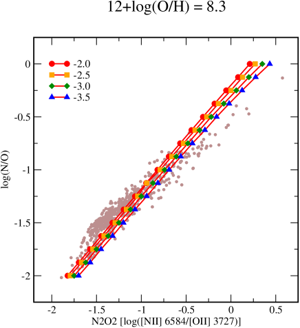
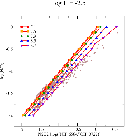
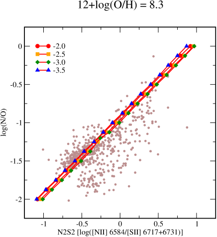
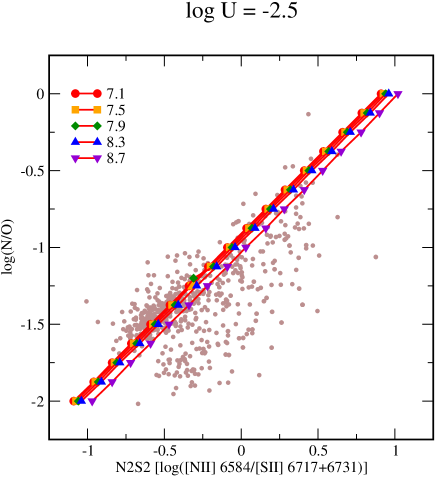
Figure 1: Relation between N/O and the N2O2 parameter in the upper row and the N2S2 parameter in the lower row for the sample of objects described in this work. Plots in the left column also show the results from models for different values of log $U$ at a fixed 12+log(O/H) = 8.3. In the right column, the models have different values of metallicity at a fixed log $U$ = -2.5.

3.2 Derivation of model-based properties

The grid of models described in the above subsection can be used to derive O/H, N/O, and log $U$ from the available optical CELs using a $\chi^{2}$-based methodology. The calculation of the model-based chemical abundances and ionisation parameter is based on the the predicted extinction-corrected intensities relative to H$\beta$ of the emission lines [O ii] 3727 Å, [O iii] 4363, 5007 Å, [N ii] 6584 Å, and [S ii] 6716+6731 Å . Notice that neither [O iii] 4959 Å nor [N ii] 6548 Å are included because the fluxes of these lines are in a fixed relation with other emission lines already considered [e.g. I(5007)/I(4959)=2.98, I(6584)/I(6548) = 3.05 (Storey & Zeippen, 2000)]

In a first step, for a given set of observed extinction-corrected emission line intensities, these are compared with the emission-lines from the models in order to estimate N/O. According to Pérez-Montero & Contini (2009), some emission-line ratios between [N ii] and other low-excitation emission-line, such as [O ii] (N2O2) or [S ii] (N2S2) depend basically on N/O. The apparent dependence of these calibrators on metallicity is mainly due to the O/H vs. N/O relation in the regime of production of secondary nitrogen. However, this relation presents a huge dispersion as N/O can also depend on star-formation history (Mollá et al., 2006) and its relation with O/H be altered with the action of hydrodynamical processes such as the inflow of metal-poor gas (Edmunds, 1990; Köppen & Hensler, 2005). These ratios also have the advantage that they do not depend on the excitation of the gas (Kewley & Dopita, 2002). In figure 1, it is shown the relation between the two considered ratios (N2O2 = log([N ii]/[O ii]); N2S2 = log([N ii]/[S ii]) and N/O for the sample of objects described in section 2 and showing the results of some models to illustrate the dependence of these ratios with O/H and with log U.

The final N/O value is then calculated as the weighted sum of the N/O values in each model using the following expression:

$$\log(N/O)_{f}=\frac{\sum_{i}\log(N/O)_{i}/\chi_{i}}{\sum_{i}1/\chi_{i}}$$ (18)

where $i$ are the different considered models from the grid, log(N/O)_i are the values of log(N/O) in each model and $\chi_{i}$ are calculated as:

$$\chi_{i}^{2}=\sum_{j}\frac{(O_{j}-T_{ji})^{2}}{O_{j}}$$ (19)

being $O_{j}$ and $T_{ji}$ the observed and model-based values, respectively, for the considered emission-line dependent ratios. In this case, N2O2, N2S2 and R_O3. R_O3 is also used since the N/O ratio also depends on $T_{e}$.

An error can also be derived using the following expression:

$$(\Delta\log(N/O))^{2}=\frac{\sum_{i}\log((N/O)_{f}-\log(N/O)_{i})^{2}/\chi_{i}}{\sum_{i}1/\chi_{i}}$$ (20)

In a second step, once N/O is estimated the grid is limited to those models with the closest N/O values to the N/O_f previously estimated (at this point, the number of models is reduced to 11$\times$21$\times$2 = 462) and a new iteration is made in order to derive the final values for O/H and log$U$ using a similar expression to that described above:

$$12+\log(O/H)_{f}=\frac{\sum_{k}(12+\log(O/H))_{k}/\chi_{k}}{\sum_{k}1/\chi_{k}}$$ (21)

$$\log U_{f}=\frac{\sum_{k}\log U_{k}/\chi_{k}}{\sum_{k}1/\chi_{k}}$$ (22)

with $k$ $<$ $i$, as the number of models was limited to those approaching the most to the derived N/O, and the values for $\chi$ are determined using the same expression as equation 19 but using as observables the ratios R_O3, [O ii]/H$\beta$, [O iii] 5007/H$\beta$, [N ii]/H$\beta$, and [S ii]/H$\beta$. The errors for the final values are also estimated using expressions similar to equation 20.

This procedure has been programmed in python language in a publicly available script called hii-chi-mistry.

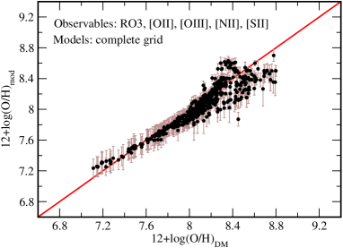
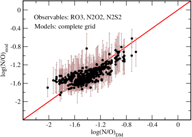
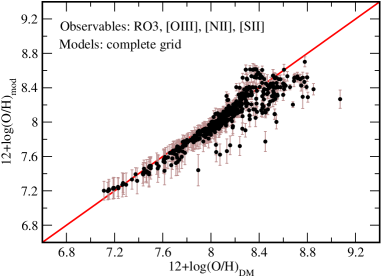
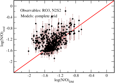
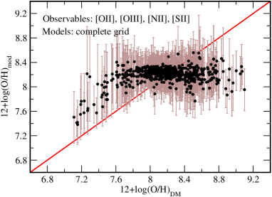
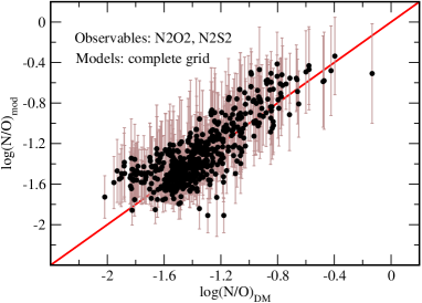
Figure 2: Comparison between the oxygen abundances (left column) and N/O ratio (right column) for the objects compiled as calculated following the direct method described in the text and using the complete grid of models. In the first row all lines ([O ii], [O iii] 4363, 5007, [N ii], and [S ii]) are used. In the middle, all lines except [O ii] and in the bottom row, all lines except [O iii] 4363. The red solid line indicates in all plots the 1:1 relation.

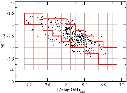
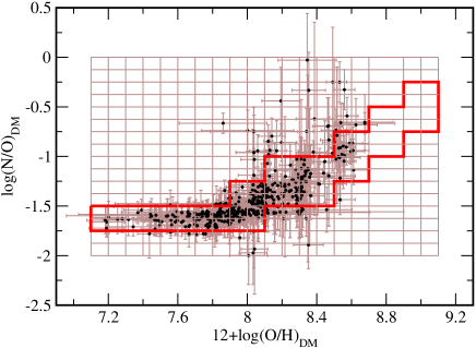
Figure 3: At left, relation between 12+log(O/H) and log $U$ for the sample of studied objects as derived using model-based values with the complete grid. At right it is shown the relation with log(N/O). The space inside the red solid line in both panels indicates the limits of the empirically limited space of models described in the text.

4 Results and discussion

4.1 Abundances using the complete grid of models

The procedure described in the previous section was followed to derive O/H, N/O, and log $U$ from the models. The derived abundances were later compared with those calculated using the direct method in the sample of objects compiled by Marino et al. (2013). The model-based abundances were estimated using the five available emission lines and the complete grid of models covering all possible excitation conditions. This excludes the objects with higher $Z$ in the sample, as their abundances were derived using other auroral lines than [O iii] 4363 Å.

In the upper panels of Figure 2 are shown the comparisons between O/H (at left) and N/O (at right) as derived using this method and the values obtained from the direct method as described in section 2. In the case of O/H, as can be seen, the agreement is very good. The average of the residuals to the 1:1 relation is lower than 0.1dex. The dispersion, estimated as the standard deviation of the residuals, is lower for low-$Z$ (0.07dex for 12+log(O/H)$<$8.0), even lower than the typical uncertainty in the derivation of the abundances following the direct method ($\sim$ 0.1dex). Howevr, this dispersion is higher for high-$Z$ (0.14dex at 12+log(O/H)$>$8.0), mainly because the determination of O/H depends strongly on the [O iii] lines, which are much brighter in the low-$Z$ regime. The dispersion in the case of N/O is of 0.15dex, and the models give slightly higher values for very low N/O values. This is likely due to deviations of the assumption made to derive this ratio (N/O $\approx$ N⁺/O⁺), which is not always valid and depends on low-excitation lines in a regime occupied mainly by low-$Z$ objects.

It is important to remark that no additional efforts were made to obtain this agreement between the abundances derived from the models and the abundances derived from the direct method, but it arises in a natural way when a consistent set of atomic data, realistic geometrical conditions and an updated code and SEDs are used.

In the middle panels of the same figure, it is shown the comparison plots of abundances when [O ii] 3727 Å is not considered in the model-based abundances. This situation happens in some spectral coverage configurations, such as, for instance, the Sloan Digital Sky Survey (SDSS) spectra for objects at a redshift lower than 0.02. As can be seen, for O/H the agreement is still very good and, in fact, the dispersions both for low-$Z$ (0.06dex) and high-$Z$ (0.12dex) are even better, always with an average value of the residuals better than 0.1dex. This is mainly due to the average O/H is not strongly affected by the relative emission of [O ii] when all the [O iii], both auroral and nebular, are available. The situation, however, is sensibly worst in the case of N/O, where a dispersion of 0.25dex is found, with a high dispersion for low N/O values. Since the main parameter to derive N/O is the N2S2 parameter, when [O ii] is not available, the contamination of the [S ii] emission lines in low-$Z$ objects make this determination very uncertain. Anyway, this dispersion is even better than the empirical dispersion of the N2S2 parameter found by Pérez-Montero & Contini (2009).

Since the main aim of this work is to provide alternative methodologies to derive abundances consistent with the direct method when no auroral line can be measured, the model-based abundances were calculated without considering the [O iii] 4363 Å emission line. Notice that in this case, all the objects compiled by Marino et al. (2013) with a direct determination of the abundance are now considered in the analysis, even those of very high-$Z$ with other auroral lines. The results of this exercise are shown both for O/H and N/O in the bottom panels of Figure 2. In the case of O/H this procedure is clearly not valid as most of the objects give a very similar value around 12+log(O/H) = 8.2 regardless of their real metallicity. Only in the case of extremely metal poor objects (XMP; 12+log(O/H) $<$ 7.65) a different trend appears. This behaviour demonstrates two things: i) [O iii] 4363 Å is the main discriminator between low-$Z$ and high-$Z$ objects independently of their excitation or geometrical conditions, and ii) very different conditions of metallicity and/or excitation lead to similar sets of emission-line fluxes if we consider with the same probability the whole space of possible values for each parameter. In the case of N/O, however, as the [O ii] emission line is now used, the agreement improves and a dispersion of 0.22dex is found, about 0.1dex better than any of the empirical calibrations of N2O2 or N2S2 found by Pérez-Montero & Contini (2009).

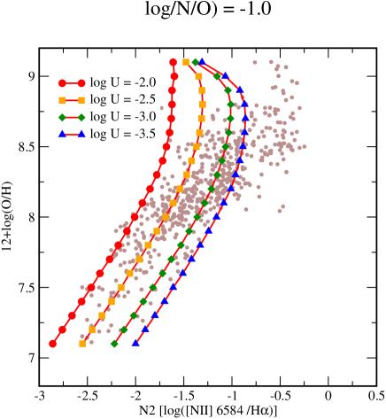
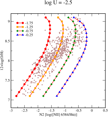
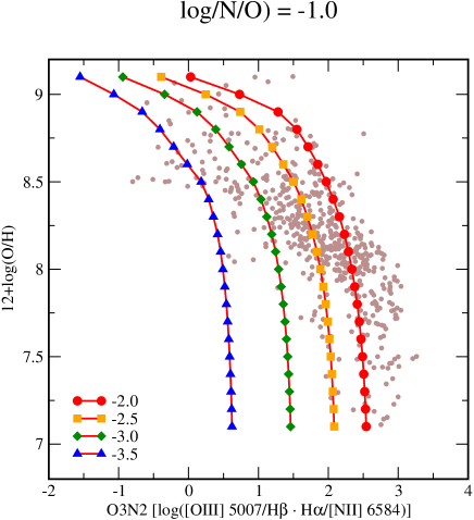
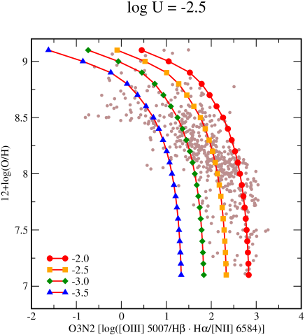
Figure 4: Relation between O/H and the N2 parameter in the upper row and with the O3N2 parameter in the lower row for the sample of objects described in this work. Plots at the left column also show the results from models for different values of log $U$ and a fixed log(N/O) = -1.0. In the right column, the models have different values of N/O at a fixed log $U$ = -2.5.

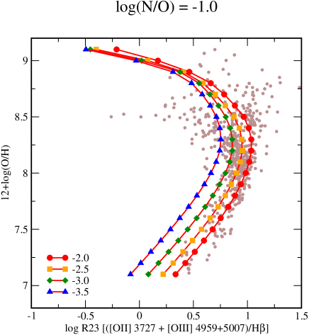
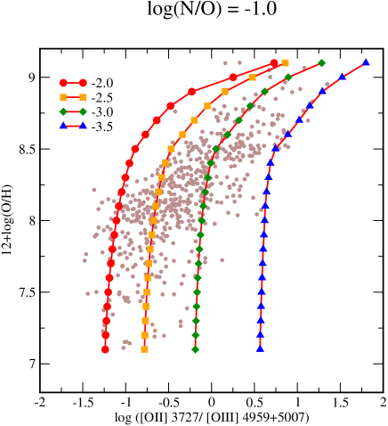
Figure 5: Relation between O/H and the R23 parameter at left and the O2O3 parameter at right for the sample of objects described in this work. Plots show the results from models for different values of log $U$ and a fixed log(N/O) = -1.0.

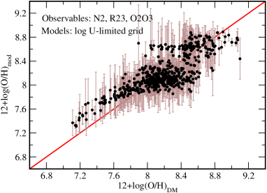
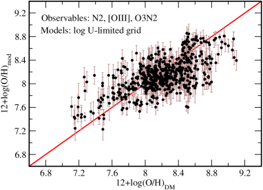
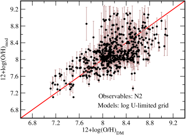
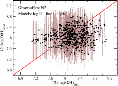
Figure 6: Comparison between the O/H derived from the direct method and the model-based values using a grid with a log $U$ empirically limited. The upper left panel uses N2, R23, and O2O3. The upper right plot uses N2, [O iii]/H$\beta$ and O3N2. The left lower panel only uses N2, but with a previous limitation of N/O using N2S2. Finally, the right lower panel shows the comparison using only N2 with no N/O restriction.

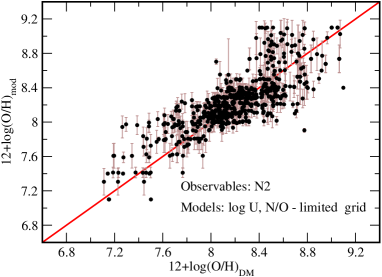
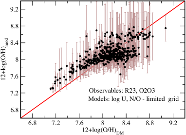
Figure 7: Comparison between O/H derived from the direct method and the model-based values using a grid empirically limited both for log $U$ and log (N/O). At left, using the N2 parameter, while at right using R23 and O2O3.

4.2 Abundances using a log $U$ empirically limited grid of models

In order to give reliable model-based abundances consistent with the direct method in absence of the [O iii] 4363 Å auroral line, and therefore let this method to work in high-$Z$, faint or high redshift star-forming objects two important assumptions are made. Firstly, the space of possible excitation conditions and metallicity is restricted empirically to fit the trend obtained for the studied sample, for which reliable values of log $U$ are obtained when using all the emission lines. This empirical relation between O/H and log $U$ is plotted in left panel of Figure 3 along with a solid line that encompasses the space of considered combinations. As can be seen, there is a trend to find higher values of log $U$ at lower metallicities, while the opposite is true at high-$Z$ (the coefficient of correlation is -0.63). Although there are objects that lie outside the assumed possible values, the majority of them lie in a region that minimizes the dispersion in the final derivation of O/H.

The second approximation that improves the agreement between the model-based O/H abundances and those derived from the direct method is to change the set of observables considered to calculate $\chi^{2}$ in equation 19. In this case, emission-line ratios known to have a clear dependence on $Z$ or log $U$ are used. This is the case of [N ii]/H$\beta$ (or equivalently [N ii]/H$\alpha$) defined as the N2 parameter (Storchi-Bergmann et al., 1994; Denicoló et al., 2002), which has a known dependence on $Z$ as can be seen in upper panels of Figure 4. The different grids of models to show the high dependence of this parameter on log $U$ and N/O as already pointed out by Pérez-Montero & Díaz (2005). Notice as well that although models predict that N2 is insensitive to O/H up to values 12+log(O/H) $\approx$ 8.5, the empirical calibrations of this parameter such as in Pettini & Pagel (2004) or Pérez-Montero & Contini (2009) can work up to values twice the solar value (around 12+log(O/H) = 9.0) because of the empirical relation between $Z$ and log $U$ or with N/O.

In the case of [O ii] and [O iii] lines the model-based abundances better agree with those from the direct method if combinations of these two lines are used as observables, such as R23 (Pagel et al., 1979), (([O ii]+[O iii])/H$\beta$), which has a bi-valuated behaviours in its dependence with $Z$ (see left panel of Figure 5) and also presents a high dependence on log $U$ and on the effective ionising temperature (Pérez-Montero & Díaz, 2005). This dependence can be partially reduced using the O2O3 parameter, defined as [O ii]/[O iii] as used by Kobulnicky et al. (1999) in their fittings of the McGaugh (1991) models or by Pilyugin & Thuan (2005) using a different formalism with their $P$ parameter. In right panel of Figure 5 it is shown the slight dependence of this ratio on $Z$ so it can be used to reduce the dependence of R23 on it.

In this way, using these three observables and the grid of models for those combinations of $Z$ and log $U$ limited by the studied sample, a much better agreement between the model-based abundances and those obtained from the direct method is obtained, as can be seen in upper left panel of Figure 6. Although the agreement is now much better, the situation is different in each metallicity regime. While for low-$Z$ (12+log(O/H) $<$ 8.0), the dispersion is lower (0.16dex), there is a systematic offset of about 0.2dex to find larger metallicities using the models. The disagreement at this regime can be possibly due to the low-excitation emission from the diffuse gas or perhaps low-velocity shocks that increase the expected flux of these lines. However, this is not critical taking into account that i) according to Pérez-Montero et al. (2013) less than 1 per cent of star-forming galaxies lie in this regime and ii) the [O iii] 4363 Å is prominent and easy to measure at these metallicities. On the contrary, for 12+log(O/H) $>$ 8.0, the agreement between the metallicities of the direct method and the model-based values is better than 0.05dex, the usual uncertainty associated with the abundances, but the dispersion enhances up to 0.19dex.

Considering again the case when [O ii] 3727 Å is not available (e.g. SDSS spectra of low-$z$ objects), the observables must be redefined. A good alternative to O2O3 is the O3N2 parameter, defined as the ratio of [O iii]/H$\beta$ and [N ii]/H$\alpha$ and used as a estimator of metallicity originally by Alloin et al. (1979). In the lower panels of Figure 4 it is shown the dependence of this parameter with oxygen abundance using the sample of compiled objects and exploring its behaviour for fixed values of log $U$ and log(N/O). The dependence of this parameter on N/O is reduced in the models for each object with the previous estimation of this ratio using the N2S2 parameter. Hence in this case for the estimation of oxygen abundance, assuming only certain values of log $U$ the observables are [N ii], [O iii], and O3N2. The metallicities obtained using this procedure are shown in the upper right panel of Figure 6. As in the case with [O ii], the agreement is better for high-$Z$ than for low-$Z$, where model-based O/H are in average 0.29dex larger. Besides, the dispersion is very similar in the two regimes (0.21dex and 0.24dex respectively), because O3N2 tends to overestimate O/H in the low-$Z$ regime.

In lower left panel of Figure 6 it is shown the comparison between the abundances from the direct method and those from the models when only [N ii] and [S ii] emission lines are used. In this case, N/O is firstly estimated using N2S2 and later, once the grid limited to the closest values of N/O and the empirical values of log $U$, O/H is also derived by means of only [N ii]/H$\beta$. The dispersion of this comparison is slightly better than the value obtained in the empirical calibration of the N2 parameter (0.31dex, Pérez-Montero & Contini (2009)), but as in the previous cases, the model-based O/H values in the low-$Z$ regime are systematically higher, with an average difference of 0.4dex, what supports the idea that low-excitation lines are overestimated in this regime.

Finally, in the right lower panel of Figure 6 it is shown the comparison using only [N ii]/H$\beta$, when no previous estimate of N/O is done. In this case, no linear correlation at all is found, as all possible values of N/O are considered in the weighted average of O/H. Therefore, no reliable estimation of O/H can be done using only [N ii] in relation to a Balmer hydrogen emission line if no previous guess about the value of N/O is done.

4.3 Abundances using a N/O empirically limited grid of models

In order to improve the agreement between the oxygen abundance derived using the direct method and the model-based values when only [N ii] emission line is available, what is the case for many high redshift star-forming objects observed in the IR, it is assumed that only certain values for N/O are valid in each metallicity regime. Of course, the use of this limited grid implies the implicit and not necessarily correct assumption that the studied object has in average the same properties that the sample studied here. However, there are cases in the literature, where combinations of N/O and O/H do not follow or lie out of the trends shown by the most part of star-forming regions/galaxies. This is the case, for instance, of green pea galaxies (Amorín et al., 2010, 2012), which present very low-$Z$ values and almost solar N/O. This, according to the authors, could be indicative that the massive star-formation processes taking place in these objects can be due to inflows of pristine gas and/or outflows of enriched material. The importance of these mechanisms should not be neglected as these are thought to be behind the empirical law found between metallicity and star formation rate (e.g. Lara-López et al. 2010; Mannucci et al. 2010; Pérez-Montero et al. 2013). Therefore, it is convenient to have a reliable estimation of N/O before deriving O/H only with the aid of [N ii] emission lines.

In the right panel of Figure 3 it is shown the relation between O/H and N/O derived using the direct method in the compiled sample of objects. The solid line encompasses the set of models considered to find abundances. As can be seen, very low values of log(N/O) at a constant value of -1.75-1.50 are obtained at 12+log(O/H) $<$ 8.0, consistently with the predictions of a production of primary N in this regime, while for high-$Z$ there is a dependence of N/O with O/H, as the main production of N has a secondary origin (e.g. Henry et al. 2000). Since no data populate the high-$Z$ regime of this diagram, it has been assumed that the linear relation between O/H and N/O extends in this regime.

Using this new limitation in the grid of models, added to that already considered between O/H and log $U$, new O/H values based only on [N ii] are derived and a better agreement is found but only for high-$Z$ with a dispersion of 0.24dex. At low-$Z$, however, a systematic offset of more than 0.4dex is found with a huge dispersion.

In the right panel of Figure 7 it is shown the comparison when only [O ii] and [O iii] strong emission lines are used, which are almost insensitive to N/O, so the N/O limited grid is more appropriate to derive reliable uncertainties. Taking again as observables R23 and O2O3 and with a previous limitation of the grid to the most probable values of log $U$, In this case, the dispersion is of only 0.19dex at all $Z$, but with an overestimation of O/H for the model-based values at 12+log(O/H) $<$ 8.0 of 0.26dex.

4.4 Application to the abundance gradient in M101

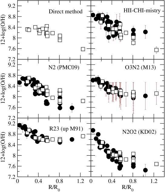
Figure 8: Galactocentric distribution of 12+log(O/H) as a function of the effective radius for the H ii regions in M101 observed by Kennicutt & Garnett (1996) (black circles) and Kennicutt et al. (2003) (white squares). The panels show the oxygen abundances as derived using the following methods from left to right and from top to bottom: the direct method, the model-based $\chi^{2}$ described in this work, the N2 parameter calibrated by Pérez-Montero & Contini (2009), the O3N2 parameter calibrated by Marino et al. (2013), the  R₂₃ calibrated by McGaugh (1991), and the N2O2 parameter calibrated by Kewley & Dopita (2002).

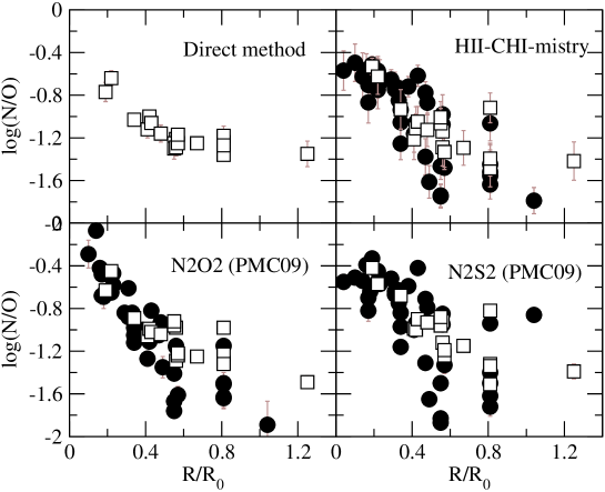
Figure 9: Galactocentric distribution of log(N/O) as a function of the effective radius for the H ii regions in M101 observed by Kennicutt & Garnett (1996) (black circles) and Kennicutt et al. (2003) (white squares). The panels show N/O ratios as derived using the following methods from left to right and from up to down: the direct method, the model-based $\chi^{2}$ described in this work, and the N2O2 and N2S2 parameters calibrated by Pérez-Montero & Contini (2009).

The study of gradients of metallicity across spiral galaxies is one of the issues where robust methods of determination of metallicity are needed, because its variation can involve in the same galaxy high- and low-$Z$ H ii regions. For instance, M101 is an object with a very prominent abundance gradient, with a variation of more than an order of magnitude in oxygen abundance from the inner to the outer regions. In order to evaluate the model-based $\chi^{2}$ method described in this work, emission-line data from the H ii regions observed by Kennicutt & Garnett (1996) and Kennicutt et al. (2003) were compiled. Later their O/H and N/O were obtained using different strong-line methods. In the case of 19 H ii regions described in Kennicutt et al. (2003) the direct method can also be applied, as these authors provide good signal-to-noise measures of different auroral lines. In this case, the expressions described in section 2 were used to re-calculate electron temperatures and ionic abundances for this sample.

In Figure 8 are shown the derived gradients in this galaxy using different methods. All of them show a prominent O/H gradient, but the behaviour can be very different depending on the used method. Using the $\chi^{2}$ model-based abundances, the maximum value is reached in the innermost regions, then the gradient is flattened for R$>$0.8$\cdot$R₀ (NGC 5471), but the oxygen abundance in the outermost position (SDH323, R/R₀ = 1.25) is sensibly lower. The oxygen abundances derived from the direct method for those H ii regions with at least one auroral line is totally consistent with this scenario, but not completely owing to the lack of points in the innermost regions and between NGC5471 and SDH323. In Figure 9 are shown the gradients for the same H ii regions for N/O. Again, the agreement between the direct method and the model-based abundances is very good, but the behaviour is sensibly different to that of O/H in the outer positions, because there is not apparent flattening and the N/O ratio for SDH323 is sensibly higher than expected. This very high N/O ratio could be consistent with an inflow of pristine gas, making the metallicity to decrease but keeping at a higher level N/O. This overabundance of N/O makes all gradients derived using [N ii] emission lines (e.g. N2, O3N2, N2O2) to very high values of $Z$ in this H ii region. In fact, the $Z$ gradient derived from N2O2 is totally similar to that of N/O. Besides, these parameters lead to strange behaviours (e.g. lower $Z$ values in the innermost regions for N2 and O3N2 and also higher $Z$ in the outer regions for O3N2) in those regimes of metallicity where they are not well calibrated. In the case of  R₂₃ , as it was calibrated using not empirically constrained models, the absolute value of oxygen is about 0.4dex higher than in the direct method. Besides, if [N ii] is used to select the upper branch calibration, the value for O/H can be even larger than in some inner positions. Finally, the N/O gradient derived from other strong-line methods, such as N2O2 or N2S2, is not very different from the models described here, but with a higher dispersion.

5 Summary and conclusions

This work analyses whether the predicted intensities of the strongest collisionally excited optical lines emitted by a gas ionised by massive stars made by photoionisation models can yield chemical abundances consistent with the direct method. For this purpose profiting the compilation made by Marino et al. (2013) of H ii regions and star-for galaxies with auroral emission-lines, their oxygen and nitrogen abundances were recalculated using the software pyneb (Luridiana et al., 2012). Besides, a large grid of cloudy (Ferland et al., 2013) photoionisation models was computed and their relative optical emission lines, O/H, N/O, and log $U$ were collected. Using a $\chi^{2}$ weighted mean procedure the chemical abundances for each observed object was recalculated using the models.

In a first step a model-based N/O is found using emission-line indicators sensitive only to this abundance ratio (i.e. N2O2, N2S2). Once N/O is enclosed, O/H and log $U$ are searched in a new iteration. This procedure, publicly available through a script called HII-CHI-mistry, leads to the following conclusions:

- The agreement between the model-based O/H and N/O abundances and those derived using the direct method is excellent when all explored lines are used ([O ii] 3727 Å, [O iii] 4363, 5007 ÅÅ, [N ii] 6584 Å, and [S ii] 6717+6731 Å all relative to H$\beta$). This agreement arises in a natural way and no additional efforts were made to force this match. The dispersion for O/H is slightly higher for 12+log(O/H) $>$ 8.0 probably owing to that the determination depends mostly on [O iii] emission lines. The agreement is quite similar even when [O ii] emission line are not considered.

- When using the grid of models covering all possible combinations of O/H, N/O, and log $U$ no reliable model-based estimation of O/H can be obtained if [O iii] 4363 Å is not taken into account. However, assuming an empirical relation between O/H and log $U$ and considering $Z$-sensitive observables in the $\chi^{2}$ method a very good agreement is obtained for 12+log(O/H) $>$ 8.0, where more than 99% of star-forming objects lie and where it is more difficult to detect the O iii] 4363Å). At low-$Z$ there is a systematic offset to obtain higher values of O/H according to models, possibly related with the contamination of the low excitation emission lines (diffuse gas and/or low velocity shocks).

- The dispersion in the comparison between model-based abundances and those obtained from the direct method is worse as a lower number of emission-lines is considered, but the obtained are always better than in other empirical calibrations using the same involved lines. When no previous estimation of N/O can be made by means of N2O2 or N2S2, additional assumptions about the O/H vs. N/O, not necessarily always true, should be made in order to obtain O/H values only from [N ii]/H$\alpha$.

- The recipes to enclose the grid of models to derive metallicities when no auroral lines are available are arbitrary and based on an empirical set of data of the local Universe. This problem is similar to the that pointed out by Stasińska (2010) for the empirical calibration of certain strong-line methods. Other recipes can be applied for the enclosing of the three input parameters (O/H, N/O, log $U$) if a limited set of lines is available and possible different scenarios are envisaged in order to arrive to realistic derivations of the chemical properties of the studied objects. Alternative recipes can be applied to the used SEDs and cluster ages used in this work.

- The use of this procedure in objects with no detection of any auroral line (faint objects, high redshift star-forming galaxies, high-$Z$ H ii regions) to derive chemical abundances can lead to values consistent with the direct method instead of strong-line methods. The use of these strong-line methods has the disadvantage that they are usually calibrated using a limited sample of objects or grids of models that do not cover all possible physical conditions. This implies that later comparisons with objects whose abundances were calculated using other methods are often inconsistent and present non-negligible offsets between them.

- The new method based on empirically constrained models was applied to study the gradients of O/H and N/O in M101. The results are totally consistent with the direct method in those regions with at least one auroral line and it is robust both in the innermost high-$Z$ and the outer low-$Z$ positions, where other strong-line methods are not well calibrated or suffer very high dependence on other ionic ratios, such as N/O.

References

- Aggarwal & Keenan (1999) Aggarwal K. M., Keenan F. P., 1999, ApJS, 123, 311
- Alloin et al. (1979) Alloin D., Collin-Souffrin S., Joly M., Vigroux L., 1979, A&A, 78, 200
- Amorín et al. (2012) Amorín R., Pérez-Montero E., Vílchez J. M., Papaderos P., 2012, ApJ, 749, 185
- Amorín et al. (2010) Amorín R. O., Pérez-Montero E., Vílchez J. M., 2010, ApJ, 715, L128
- Asplund et al. (2009) Asplund M., Grevesse N., Sauval A. J., Scott P., 2009, ARA&A, 47, 481
- Bresolin (2007) Bresolin F., 2007, ApJ, 656, 186
- Bresolin et al. (2009) Bresolin F., Gieren W., Kudritzki R.-P., Pietrzyński G., Urbaneja M. A., Carraro G., 2009, ApJ, 700, 309
- Chabrier (2003) Chabrier G., 2003, ApJ, 586, L133
- Charlot & Longhetti (2001) Charlot S., Longhetti M., 2001, MNRAS, 323, 887
- Denicoló et al. (2002) Denicoló G., Terlevich R., Terlevich E., 2002, MNRAS, 330, 69
- Dors et al. (2013) Dors O. L. et al., 2013, MNRAS, 432, 2512
- Dors et al. (2011) Dors, Jr. O. L., Krabbe A., Hägele G. F., Pérez-Montero E., 2011, MNRAS, 415, 3616
- Edmunds (1990) Edmunds M. G., 1990, MNRAS, 246, 678
- Esteban et al. (2009) Esteban C., Bresolin F., Peimbert M., García-Rojas J., Peimbert A., Mesa-Delgado A., 2009, ApJ, 700, 654
- Fang & Liu (2013) Fang X., Liu X.-W., 2013, MNRAS, 429, 2791
- Ferland et al. (2013) Ferland G. J. et al., 2013, RMxAA, 49, 137
- Firnstein & Przybilla (2012) Firnstein M., Przybilla N., 2012, A&A, 543, A80
- Garnett (1992) Garnett D. R., 1992, AJ, 103, 1330
- Hägele et al. (2008) Hägele G. F., Díaz Á. I., Terlevich E., Terlevich R., Pérez-Montero E., Cardaci M. V., 2008, MNRAS, 383, 209
- Henry et al. (2000) Henry R. B. C., Edmunds M. G., Köppen J., 2000, ApJ, 541, 660
- Hudson et al. (2012) Hudson C. E., Ramsbottom C. A., Scott M. P., 2012, ApJ, 750, 65
- Kennicutt et al. (2003) Kennicutt, Jr. R. C., Bresolin F., Garnett D. R., 2003, ApJ, 591, 801
- Kennicutt & Garnett (1996) Kennicutt, Jr. R. C., Garnett D. R., 1996, ApJ, 456, 504
- Kewley & Dopita (2002) Kewley L. J., Dopita M. A., 2002, ApJS, 142, 35
- Kewley & Ellison (2008) Kewley L. J., Ellison S. L., 2008, ApJ, 681, 1183
- Kobulnicky et al. (1999) Kobulnicky H. A., Kennicutt, Jr. R. C., Pizagno J. L., 1999, ApJ, 514, 544
- Köppen & Hensler (2005) Köppen J., Hensler G., 2005, A&A, 434, 531
- Lara-López et al. (2010) Lara-López M. A. et al., 2010, A&A, 521, L53
- Liu (2010) Liu X., 2010, ArXiv e-prints 1001.3715
- Luridiana et al. (2012) Luridiana V., Morisset C., Shaw R. A., 2012, in IAU Symposium, Vol. 283, IAU Symposium, pp. 422–423
- Mannucci et al. (2010) Mannucci F., Cresci G., Maiolino R., Marconi A., Gnerucci A., 2010, MNRAS, 408, 2115
- Marino et al. (2013) Marino R. A. et al., 2013, A&A, 559, A114
- Mathis et al. (1977) Mathis J. S., Rumpl W., Nordsieck K. H., 1977, ApJ, 217, 425
- McGaugh (1991) McGaugh S. S., 1991, ApJ, 380, 140
- Mollá et al. (2009) Mollá M., García-Vargas M. L., Bressan A., 2009, MNRAS, 398, 451
- Mollá et al. (2006) Mollá M., Vílchez J. M., Gavilán M., Díaz A. I., 2006, MNRAS, 372, 1069
- Morisset (2013) Morisset C., 2013, pyCloudy: Tools to manage astronomical Cloudy photoionization. Astrophysics Source Code Library
- Nicholls et al. (2012) Nicholls D. C., Dopita M. A., Sutherland R. S., 2012, ApJ, 752, 148
- Pagel et al. (1979) Pagel B. E. J., Edmunds M. G., Blackwell D. E., Chun M. S., Smith G., 1979, MNRAS, 189, 95
- Peimbert (1967) Peimbert M., 1967, ApJ, 150, 825
- Pérez-Montero & Contini (2009) Pérez-Montero E., Contini T., 2009, MNRAS, 398, 949
- Pérez-Montero et al. (2013) Pérez-Montero E. et al., 2013, A&A, 549, A25
- Pérez-Montero & Díaz (2005) Pérez-Montero E., Díaz A. I., 2005, MNRAS, 361, 1063
- Pérez-Montero & Díaz (2007) Pérez-Montero E., Díaz Á. I., 2007, MNRAS, 377, 1195
- Pérez-Montero et al. (2010) Pérez-Montero E., García-Benito R., Hägele G. F., Díaz Á. I., 2010, MNRAS, 404, 2037
- Pettini & Pagel (2004) Pettini M., Pagel B. E. J., 2004, MNRAS, 348, L59
- Pilyugin & Thuan (2005) Pilyugin L. S., Thuan T. X., 2005, ApJ, 631, 231
- Pradhan et al. (2006) Pradhan A. K., Montenegro M., Nahar S. N., Eissner W., 2006, MNRAS, 366, L6
- Simón-Díaz & Stasińska (2011) Simón-Díaz S., Stasińska G., 2011, A&A, 526, A48
- Stasińska (2010) Stasińska G., 2010, in IAU Symposium, Vol. 262, IAU Symposium, Bruzual G. R., Charlot S., eds., pp. 93–96
- Storchi-Bergmann et al. (1994) Storchi-Bergmann T., Calzetti D., Kinney A. L., 1994, ApJ, 429, 572
- Storey & Zeippen (2000) Storey P. J., Zeippen C. J., 2000, MNRAS, 312, 813
- Tayal (2007) Tayal S. S., 2007, ApJS, 171, 331
- Tayal (2011) Tayal S. S., 2011, ApJS, 195, 12
- Tayal & Zatsarinny (2010) Tayal S. S., Zatsarinny O., 2010, ApJS, 188, 32
- Tsamis & Péquignot (2005) Tsamis Y. G., Péquignot D., 2005, MNRAS, 364, 687