Scalable Matting: A Sub-linear Approach

Abstract

Natural image matting, which separates foreground from background, is a very important intermediate step in recent computer vision algorithms. However, it is severely underconstrained and difficult to solve. State-of-the-art approaches include matting by graph Laplacian, which significantly improves the underconstrained nature by reducing the solution space. However, matting by graph Laplacian is still very difficult to solve and gets much harder as the image size grows: current iterative methods slow down as $\mathcal{O}\left(n^{2}\right)$ in the resolution $n$. This creates uncomfortable practical limits on the resolution of images that we can matte. Current literature mitigates the problem, but they all remain super-linear in complexity. We expose properties of the problem that remain heretofore unexploited, demonstrating that an optimization technique originally intended to solve PDEs can be adapted to take advantage of this knowledge to solve the matting problem, not heuristically, but exactly and with sub-linear complexity. This makes ours the most efficient matting solver currently known by a very wide margin and allows matting finally to be practical and scalable in the future as consumer photos exceed many dozens of megapixels, and also relieves matting from being a bottleneck for vision algorithms that depend on it.

1 Introduction

The problem of extracting an object from a natural scene is referred to as alpha matting. Each pixel $i$ is assumed to be a convex combination of foreground and background colors $F_{i}$ and $B_{i}$ with $\alpha_{i}\in[0,1]$ being the mixing coefficient:

$$I_{i}=\alpha_{i}F_{i}+(1-\alpha_{i})B_{i}.$$ (1)

Besides the motivation to solve the matting problem for graphics purposes like background replacement, there are many computer vision problems that use matting as an intermediate step like dehazing [1], deblurring [2], and even tracking [3] to name a few.

Since there are 3 unknowns to estimate at each pixel, the problem is severely underconstrained. Most modern algorithms build complex local color or feature models in order to estimate $\alpha$. One of the most popular and influential works is [4], which explored graph Laplacians based on color similarity as an approach to solve the matting problem.

The model that most Laplacian-based matting procedures use is

$$p\left(I\mid\alpha\right) \propto\exp\left(-\frac{1}{2}\left\lVert\alpha\right\rVert^{2}_{L}\right)\;\text{and}$$ (2)

$$\alpha_{\text{MLE}} =\arg\max_{\alpha}p(I\mid\alpha),$$ (3)

where $L$ is a per-pixel positive semi-definite matrix that represents a graph Laplacian over the pixels, and $\left\lVert\alpha\right\rVert^{2}_{L}=\langle\alpha,L\alpha\rangle$ is the induced norm. Typically $L$ is also very sparse as the underlying graph representing the pixels is connected only locally to its immediate spatial neighbors, and $L$ is directly related to the adjacency matrix (see §2.1). However, $L$ always has positive nullity (several vanishing eigenvalues), meaning that the estimate (3) is not unique. So, user input is required to provide a prior to resolve the ambiguity. A crude prior that is frequently used is:

$$p(\alpha)\propto\begin{cases}1&\text{if}\;\alpha\;\text{is consistent with user input}\\ 0&\text{o.w.}\end{cases}.$$ (4)

This is often implemented by asking the user to provide “scribbles” to constrain some pixels of the matte to 1 (foreground) or 0 (background) by using foreground and background brushes to manually paint over parts of the image. We give an example in Fig. 1.

To get the constrained matting Laplacian problem into the linear form $A\alpha=f$, one can choose

$$A \stackrel{{\scriptstyle\Delta}}{{=}}(L+\gamma C),\;\text{and}$$

$$f \stackrel{{\scriptstyle\Delta}}{{=}}\gamma g,$$ (5)

where $C$ is diagonal, $C_{ii}=1$ if pixel $i$ is user-constrained to value $g_{i}$ and 0 o.w., and $\gamma$ is the Lagrange multiplier for those constraints. If there are $n$ pixels in the image $I$, then $A$ is $n\times n$ with $\operatorname{nnz}(A)\in\mathcal{O}\left(n\right)$.

Since $A$ is symmetric and positive definite (with enough constraints), it is tempting to solve the system by a Cholesky decomposition. However, this is simply impossible on a modest-size image on modern consumer hardware, since such decompositions are dense and rapidly exhaust gigabytes of memory when the resolution is larger than around 10,000 pixels ($316\times 316$). The reason is that these decompositions are dense, though the input matrix is sparse. So, if each entry is 8 B, then the number of GB required to store the decomposition of a sparse $10,000\times 10,000$ system is $8(10,000^{2})/(2(10^{9}))=40$ GB. Further, although they are fast for small systems, the time complexity is $\mathcal{O}\left(n^{3}\right)$, which will eventually dominate, even if we have unlimited memory.

It is also tempting to incorporate the user-provided equality constraints directly, which reduces the system size by the number of constrained pixels. In order to solve this reduced system in memory would still require the number of unconstrained pixels to be less than about 40k on a system with 8 GB memory. This is also impractical, because it places the burden on the user or some other automated algorithm to constrain at least 95% of a megapixel image, and much more at higher resolutions.

There are a number of methods to approximately solve the problem by relying on good heuristics about natural images and the extracted alpha mattes themselves. For example, [5] split the problem into multiple independent pieces, and [6] perform segmentation to reduce the problem size.

If we desire to avoid heuristics and obtain an exact solution, then it is necessary to resort to more memory-efficient iterative algorithms, which can take advantage of the sparsity of $A$. There are many traditional iterative methods for solving the full-scale matting problem such as the Jacobi method, succesive over-relaxation, gradient descent, and conjugate gradient descent. Although memory-efficient, they are all quite slow, especially as the resolution increases. There is a fundamental reason for this: the condition number of the system grows as $\mathcal{O}\left(n^{2}\right)$ in the number of pixels, making these linear solvers also slow down at something like $\mathcal{O}\left(n^{2}\right)$.

Even the “fast” matting methods only improve the complexity by a constant factor. For example, by splitting the problem into $k$ independently-solved pieces, [5] changes the complexity to $\mathcal{O}\left(k(n/k)^{2}\right)=\mathcal{O}\left(n^{2}/k\right)=\mathcal{O}\left(n^{2}\right)$. [6] at first seems to solve the problem efficiently by segmenting the problem into $m\ll n$ segments where $m$ is constant w.r.t. $n$. However, the complexity is hidden in performing the segmentation, which is still at least $\mathcal{O}\left(n^{2}\right)$. No matter what engineering we do to reduce these constant factors, it is the underlying solvers that prevent us from improving the overall complexity to get an algorithm that is truly scalable.

Iterative methods can be characterized by their per-iteration error reduction ratio, which is called the convergence rate. The closer to 0, the better, and the closer to 1, the worse the method is. Currently-used iterative methods are bound by the condition number of the system, and therefore have convergence rates like $1-\mathcal{O}\left(n^{-2}\right)$, slowing down dramatically as the problem gets large (§2.2).

There is a property of mattes of natural images that has not been fully exploited: they tend to be constant almost everywhere (Fig. 1.c). In fact, for opaque foreground objects, the only regions that contribute to the objective function are the pixels on the edge of the object. Computation on non-boundary pixels is wasteful. Further, as the resolution grows, the ratio of the number of edge pixels to the rest of the pixels goes to zero. This means if we can find a solver that exploits these properties to focus on the boundary, it should be more efficient as $n$ grows. Since these properties hold independent of the choice of the Laplacian, such a solver would be general and much more natural than the heuristics currently applied to the Laplacian itself.

In this paper, we propose the use of multigrid algorithms to efficiently solve the matting problem by fully exploiting these properties. Multigrid methods are briefly mentioned by [7] and [5] for solving the matting problem, concluding that the irregularity of the Laplacian is too much for multigrid methods to overcome. We thoroughly analyze those claims, and find that conclusion to be premature. This paper shows for the first time a solver of sub-linear time complexity, ($\mathcal{O}\left(n^{0.752}\right)$ average case) that solves the full-scale problem without heuristics, works on any choice of matting Laplacian, sacrifices no quality, and finally provides a scalable solution for natural image matting on ever larger images.

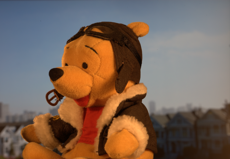
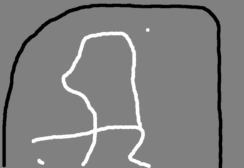
(a)	(b)
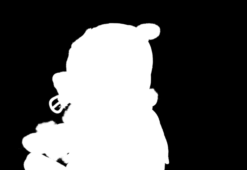
(c)

Figure 1: Input image (a). User constraints or “scribbles” (b). Desired output matte (c).

2 Background

2.1 The Matting Laplacian

Matting by graph Laplacian is a common technique in matting literature [4, 8, 5, 9]. Laplacians play a significant role in graph theory and have wide applications, so we will take a moment to describe them here. Given an undirected graph $G=(V,E)$, the adjacency matrix of $G$ is a matrix $A^{G}_{ij}$ of size $\lvert V\rvert\times\lvert V\rvert$ that is positive $\forall v_{i}v_{j}\in E$. $A^{G}_{ij}$ is the “weight” on the graph between $v_{i}$ and $v_{j}$. Further define $D^{G}_{ii}=d(v_{i})=\sum_{j\neq i}A^{G}_{ij}$ to be a diagonal matrix containing the degree of $v_{i}$, and let $x$ be a real-valued function $V\rightarrow\mathbb{R}$. The Laplacian $L^{G}=D^{G}-A^{G}$ defines the quadratic form on the graph

$$q(x)\stackrel{{\scriptstyle\Delta}}{{=}}x^{T}L^{G}x=\sum_{v_{i}v_{j}\in E}A^{G}_{ij}(x_{i}-x_{j})^{2}.$$ (6)

By construction, it is easy to see that $L^{G}$ is real, symmetric, and positive semi-definite, and has $\boldsymbol{1}$ (the constant vector) as its first eigenvector with eigenvalue $\lambda_{1}=0$.

This quadratic form plays a crucial role in matting literature, where the graph structure is the grid of pixels, and the function over the vertices is the alpha matte $\alpha\in[0,1]^{\lvert V\rvert}$. By designing the matrix $A^{G}_{ij}$ such that it is large when we expect $\alpha_{i}$ and $\alpha_{j}$ are the same and small when we expect they are unrelated, then minimizing $q(\alpha)$ over the alpha matte is finding a matte that best matches our expectations. The problem is that, as we have shown, one minimizer is always the constant matte $\boldsymbol{1}$, so extra constraints are always required on $\alpha$.

Many ways have been proposed to generate $A^{G}$ so that a good matte can be extracted. In [10], $A^{G}$ is constructed to represent simple 4-neighbor adjacency. In [4], $A^{G}_{ij}$ is given as

$$\sum_{k\mid(i,j)\in w_{k}}\frac{1}{\lvert w_{k}\rvert}\left(1+\langle I_{i}-\mu_{k},I_{j}-\mu_{k}\rangle_{(\Sigma_{k}+\epsilon I)^{-1}}\right),$$ (7)

where $w_{k}$ is a spatial window of pixel $k$, $\mu_{k}$ is the mean color in $w_{k}$, and $\Sigma_{k}$ is the sample color channel covariance matrix in $w_{k}$.

In [8], the color-based affinity in eq. (7) is extended to an infinite-dimensional feature space by using the kernel trick with a gaussian kernel to replace the RGB Mahalanobis inner product, and [9] does something similar on patches of colors instead of single colors, with more flexibility in the model and assumptions. [11] provides many other uses of graph Laplacians, not only in matting or segmentation, but also in other instances of transductive learning. [12] demonstrated that [4]’s Laplacian intrinsically has a nullity of 4, meaning that whatever prior is used, it must provide enough information for each of the 4 subgraphs and their relationships to each other in order to find a non-trivial solution.

No matter how we choose $A^{G}$, the objective is to minimize $q(x)$ subject to some equality constraints (e.g. the user scribbles mentioned above). Although it is simply a constrained quadratic program, it becomes very difficult to solve as the system size grows past millions of pixels, and necessitates investigation to be practical.

2.2 Relaxation

No matter what method we choose to construct the matting Laplacian, we end up with a large, sparse, ill-conditioned problem. There are a number of methods to solve large linear systems $Au=f$ for $u$. Traditional methods include Gauss-Seidel and successive over-relaxation (SOR). These are relaxation methods, where the iteration is of the affine fixed-point variety:

$$u\leftarrow G(u)\stackrel{{\scriptstyle\Delta}}{{=}}Ru+g.$$ (8)

If $\hat{u}$ is the solution, it must be the case that it is a fixed point of the iteration: $\hat{u}=R\hat{u}+g$. For analysis, we can define the error and residual vectors

$$e \stackrel{{\scriptstyle\Delta}}{{=}}\hat{u}-u\;\text{and}$$

$$r \stackrel{{\scriptstyle\Delta}}{{=}}f-Au$$

so that original problem is transformed to $Ae=r$. We can then see that

$$e \leftarrow Re\;\text{i.e.}$$

$$e^{\text{new}} =Re$$ (9)

is the iteration with respect to the error. This tells us that the convergence rate $\left\lVert e^{\text{new}}\right\rVert/\left\lVert e\right\rVert$ is bounded from above by the spectral radius $\rho(R)$. So, a simple upper bound for the error reduction at iteration $j$ is $\left\lVert e^{j}\right\rVert/\left\lVert e^{1}\right\rVert\leq\rho(R)^{j}$. So, for quickest convergence and smallest error, we want $\rho(R)$ to be much less than 1.

For our kind of problems (discrete Laplace operators), the Jacobi method’s iteration matrix $R_{J}$ gives a convergence rate of $\rho(R_{J})\leq 1-a/n^{2}$, where $n$ is the number of variables and $a$ is a constant. The Gauss-Seidel iteration matrix gives $\rho(R_{G})\leq\rho(R_{J})^{2}$, meaning it converges twice as fast as the Jacobi method. There are similar results for SOR, gradient descent, and related iterative methods.

Recall $\rho(R)=\max_{i}\left\lvert\mu_{i}\right\rvert$, where $\mu_{i}$ are the eigenvalues of $R$. So, to analyze the convergence, we need to understand the eigenvalues. We can decompose the error $e$ in the basis of eigenvectors $v_{i}$ of $R$:

$$e^{1}=\sum_{i=1}^{n}a_{i}v_{i}.$$ (10)

After $j$ iterations, we have

$$e^{j}=\sum_{i=1}^{n}\mu_{i}^{j}a_{i}v_{i}.$$ (11)

So, the closer $\mu_{i}$ is to zero, the faster the $v_{i}$ component of $e$ converges to 0. For Laplace operators, we explain in the example below that $i$ corresponds to a generalization of frequency, and $\rho(R)=\mu_{1}$, the lowest “frequency” eigenvalue.

Since $\mu_{1}$ is closest to 1, the $v_{1}$ (low-frequency) component dominates the convergence rate, while the higher-frequency components are more easily damped out (for this reason, relaxation is often called smoothing). Further, we explain that the convergence rate rapidly approaches 1 as $n$ grows. To break this barrier, we need a technique that can handle the low-frequencies just as well as the high frequencies.

2.2.1 Motivating Example

To understand why, let us take the 1D Laplace equation with Dirichlet boundary conditions as an example from [13]:

$$Au =f,\;\text{where}$$ (12)

$$A =-\nabla^{2},\;\text{and}$$

$$f =0$$

$$\text{s.t.}\;u_{0} =u_{n+1}=0.$$

This problem has two fixed variables $u_{0}$ and $u_{n+1}$, and $n$ free variables $u_{1},\dotsc,u_{n}$. $A$ is $n\times n$ and is the operator $-\nabla^{2}$ corresponding to convolution with the discrete Laplace kernel $[-1,2,-1]$. The underlying graph in this case has node $i$ adjacent to nodes $i-1$ and $i+1$. We use this example because it is directly analagous to matting, but easier to analyze. Notice that the problem has a unique solution $u=0$.

Without loss of generality, we assume that the $u_{i}$ are spaced $h=1/(n+1)$ units apart, corresponding to a continuous function $u$ whose domain is the unit interval $[0,1]$. We write the problem in Eq. (12) as

$$-u_{i-1}+2u_{i}-u_{i+1}=0,\;\forall 1\leq i\leq n,$$ (13)

which naturally incorporates the constraints, and gives us a symmetric, banded, positive-definite matrix,

$$A=\left[\begin{array}[]{rrrrr}2&-1&0&0&\\ -1&2&-1&0&\\ 0&-1&2&-1&\\ &&\ddots&\ddots&\ddots\end{array}\right].$$ (18)

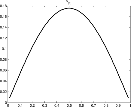
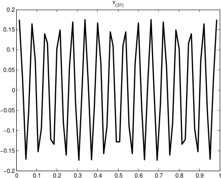
Figure 2: Eigenfunctions of $A$ when $n=64$.

For this problem, it is a simple exercise to show that the eigenfunctions and eigenvalues of $A$ are

$$v_{(k)i}^{h} =\sin(k\pi ih)/h,\;\text{and}$$ (19)

$$\lambda_{i}^{h} =2-2\cos(\pi ih).$$ (20)

Notice that $i$ directly corresponds to the frequency of the eigenfunctions. In fact, graph Laplacians always admit a decomposition into a basis of oscillatory mutually-orthogonal eigenfunctions. This gives us a general notion of frequency that applies to any graph. Two of the eigenfunctions of this particular example are depicted in Fig. 2, and exactly correspond to our usual interpretation of frequency as Eq. (19) shows.

The condition number $\kappa(A)$ tells us how difficult it is to accurately solve a problem involving $A$ (the smaller, the better). Using the small angle approximation, we can see that $\lambda_{1}^{h}\approx\pi^{2}h^{2}$ and $\lambda_{n}^{h}\approx 4-h^{2}$. This gives a condition number $\kappa(A)=\lambda_{n}^{h}/\lambda_{1}^{h}\approx 4/(\pi^{2}h^{2})=4(n+1)^{2}/\pi^{2}$, meaning that the condition number is $\mathcal{O}\left(n^{2}\right)$. This implies the difficulty of solving the problem gets much worse the more variables we have. Notice the cause is that the lowest-frequency eigenvalue $\lambda_{1}^{h}\rightarrow 0$ as $n\rightarrow\infty$, which makes the condition number grow unbounded with $n$. These low-frequency modes are the primary problem we have to grapple if we wish to solve large graph problems efficiently.

For the Jacobi relaxation, the iteration matrix is

$$R_{J}=D^{-1}(L+U),$$ (21)

where $D$, $L$ (not to be confused with the Laplacian) and $U$ are the diagonal, lower-, and upper-triangular parts of $A$. It is a simple exercise to prove that $\rho(R_{J})\approx 1-\pi^{2}h^{2}/2$ since its eigenvalues are $\mu_{i}^{h}=\cos(\pi ih)$, where $i$ again corresponds to the frequency of the eigenfunction $i$. Recall from §2.2, we want $\rho(R)\ll 1$ for fast convergence. Due to Eq. (9), this means that if the error $e$ has any low-frequency components, they will converge like $(1-\pi^{2}h^{2}/2)^{j}$ (if $j$ is the iteration). This becomes extremely slow as $n\rightarrow\infty$, $h\rightarrow 0$, and the spectral radius $\rho(R_{J})\rightarrow 1$.

Gauss-Seidel is somewhat better. Its iteration matrix is

$$R_{G}=(D-L)^{-1}U.$$ (22)

Its eigenvalues are $\mu_{i}^{h}=\cos^{2}(\pi ih)$ for this problem, giving $\rho(R_{G})\leq\rho(R_{J})^{2}$. However, it still has the same basic issue of slow convergence on low-frequency modes, which gets worse with increasing problem size $n$.

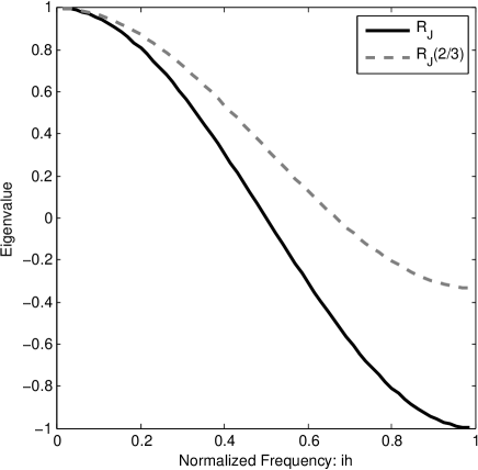
Figure 3: Eigenvalues of $R_{J}$ and $R_{J}(2/3)$. The latter has high-frequency eigenvalues much closer to 0, giving improved high-frequency convergence.

As given, both of these methods also have problems with high-frequency modes. This can be ameliorated with damping:

$$R(\omega) \stackrel{{\scriptstyle\Delta}}{{=}}(1-\omega)I+\omega R,\;\text{giving}$$ (23)

$$\mu_{i}(\omega) =1-\omega+\omega\mu_{i},$$ (24)

where $\omega$ is the damping parameter, and $\mu_{i}$ are the eigenvalues of $R$. By choosing $\omega=2/3$ for the Jacobi method, the convergence rate for the high-frequency modes significantly improves as the corresponding eigenvalues decrease in magnitude from near unity to about $1/3$, as demonstrated in Fig. 3. A similar effect occurs with Gauss Seidel.

Gradient descent behaves quite similarly to the Jacobi iteration, and while conjugate gradient (CG) is a bit harder to analyze in this fashion, it also displays the same problems in practice. The low-frequency eigenmodes of this problem are a serious issue if we want to develop a fast solver.

Though we have described a very simple system, we have analagous problems in matting, just that the constraints are user-supplied and the Laplacian is usually data-dependent. For matting, most methods have sidestepped this problem by relying on very dense constraints to resolve most of the low-frequency components. No one has yet proposed a solver for Laplacian-based matting which can handle the low-frequency modes efficiently as the resolution increases and as constraints become sparse.

2.3 Multigrid Methods

Multigrid methods are a class of solvers that attempt to fix the problem of slow low-frequency convergence by integrating a technique called nested iteration. The basic idea is that, if we can downsample the system, then the low-frequency modes in high-resolution will become high-frequency modes in low-resolution, which can be solved with relaxation. A full treatment is given in [13].

Without loss of generality, we can assume for simplicity that the image is square, so that there are $N$ pixels along each axis, $n=N^{2}$ total pixels, with $h=1/(N-1)$ being the spacing between the pixels, corresponding to a continuous image whose domain is $[0,1]^{2}$. Since we will talk about different resolutions, we will let $n_{h}=(1/h+1)^{2}$ denote the total number of pixels when the resolution is $h$. We will also assume for simplicity that the spacings $h$ differ by powers of 2, and therefore the number of pixels differ by powers of 4. The downsample operators are linear and denoted by $I_{h}^{2h}:\mathbb{R}^{n_{h}}\rightarrow\mathbb{R}^{n_{2h}}$, and the corresponding upsample operators are denoted by $I_{2h}^{h}=(I_{h}^{2h})^{T}$. The choice of these transfer operators is application-specific, and we will discuss that shortly.

The idea of nested iteration is to consider solutions to

$$I_{h}^{2h}Au^{h}=I_{h}^{2h}f^{h},$$ (25)

that is to say a high-resolution solution $u^{h}$ that solves the downsampled problem exactly. Such a system is over-determined, so we can restrict our search to coarse-grid interpolants $u^{h}=I_{2h}^{h}u^{2h}$. So, we get

$$I_{h}^{2h}AI_{2h}^{h}u^{2h}=I_{h}^{2h}f^{h}.$$ (26)

Since $I_{2h}^{h}=(I_{h}^{2h})^{T}$, we can see that $A^{2h}\stackrel{{\scriptstyle\Delta}}{{=}}I_{h}^{2h}AI_{2h}^{h}$ is the equivalent coarse system. Of course we can repeat this to get $A^{4h}$ and so on. The advantage of a smaller system is two-fold: first, the system is smaller and therefore is more efficient to iterate on, and second, the smaller system will converge faster due to better conditioning.

So, supposing we can exactly solve, say, $u^{16h}$, then we can get an initial approximation $u_{0}^{h}=I_{2h}^{h}I_{4h}^{2h}\ldots I_{16h}^{8h}u^{16h}$. This is the simple approach taken by many pyramid schemes, but we can do much better. The strategy is good if we have no initial guess, but how can this be useful if we are already given $u_{0}^{h}$? The modification is subtle and important: iterate on the error $e$ instead of the solution variable $u$.

Algorithm 1 Nested Iteration

1:$r^{h}\leftarrow f^{h}-A^{h}u^{h}$

2:$r^{2h}\leftarrow I_{h}^{2h}r^{h}$

3:Estimate $A^{2h}e^{2h}=r^{2h}$ for $e^{2h}$ using $e_{0}^{2h}=0$.

4:$u^{h}\leftarrow u^{h}+I_{2h}^{h}e^{2h}$

Of course, step 3 suggests a recursive application of Alg. 1. Notice that if the error is smooth ($e^{h}\approx I_{2h}^{h}e^{2h}$), then this works very well since little is lost by solving on the coarse grid. But, if the error is not smooth, then we make no progress. In this respect, nested iteration and relaxation are complementary, so it makes a lot of sense to combine both. This is called v-cycle, and is given in Alg. 2. A visualization of the algorithm is shown in Fig. 4.

Algorithm 2 V-Cycle

1:function vcycle($u^{h}$,$f^{h}$)

2:     if $h=H$ then return exact solution $u^{h}$

3:     end if

4:     Relax on $A^{h}\mathbf{u}^{h}=f^{h}$

5:     $r^{h}\leftarrow f^{h}-A^{h}u^{h}$ (compute residual)

6:     $e^{2h}\leftarrow$ VCYCLE($e^{2h}=0$,$I_{h}^{2h}r^{h}$) (estimate correction)

7:     $u^{h}\leftarrow u^{h}+I_{2h}^{h}e^{2h}$. (apply correction)

8:     Relax on $A^{h}\mathbf{u}^{h}=f^{h}$

9:     return $u^{h}$

10:end function

The idea of multigrid is simple: incorporating coarse low-resolution solutions to the full-resolution scale. The insight is that the low-resolution parts propagate information quickly, converge quickly, and are cheap to compute due to reduced system size.

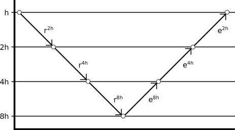
Figure 4: Visualization of the v-cycle schedule. The iteration recursively passes down the residual to the next lowest resolution and retrieves the error (corresponding to lines 6 & 7 in Alg. 2). The V shape is the reason for the name.

When the problem has some underlying geometry, multigrid methods can provide superior performance. It turns out that this is not just heuristic, but also has nice analytic properties. On regular grids, v-cycle is provably optimal, and converges in a constant number of iterations with respect to the resolution [14].

It is also important to see that the amount of work done per iteration is $\mathcal{O}\left(n\right)$ in the number of variables. To see this, we can take relaxation on the highest resolution to be 1 unit of work. Looking at Alg. 2, there is one relaxation call, followed by recursion, followed by another relaxation call. In our case, the recursion operates on a problem at $1/4$ size, so we have the total work as $W(n)=1+W(\frac{n}{4})+1=2+W(\frac{n}{4})$. In general, the relaxation costs $n_{h}/N$, and the expression becomes $W(n_{h})=2\frac{n_{h}}{n}+W(\frac{n_{h}}{4})$. If we continue the expression, $W(n)=2+2\frac{1}{4}+2\frac{1}{16}+\cdots=2\sum_{i=0}^{\infty}\frac{1}{4}^{n}$, which converges to $W(n)=8/3$. In other words, the work done for v-cycle is just a constant factor of the work done on a single iteration of the relaxation at full resolution. Since the relaxation methods chosen are usually $\mathcal{O}\left(n\right)$, then a single iteration of v-cycle is also $\mathcal{O}\left(n\right)$. So, we get a lot of performance without sacrificing complexity.

V-cycle (and the similar w-cycle) multigrid methods work well when the problem has a regular geometry that allows construction of simple transfer operators. When the geometry becomes irregular, the transfer operators must also adapt to preserve the performance benefits. When the geometry is completely unknown or not present, algebraic multigrid algorithms can be useful, which attempt to automatically construct problem-specific operators, giving a kind of “black box” solver.

2.4 Multigrid (Conjugate) Gradient Descent

Here, we describe a relatively new type of multigrid solver from [15] that extends multigrid methods to gradient and conjugate gradient descent. Please note that our notation changes here to match that of [15] and to generalize the notion of resolution.

If the solution space has a notion of resolution on $\ell$ total levels, with downsample operators $I_{\ell}^{i}:\mathbb{R}^{n_{\ell}}\rightarrow\mathbb{R}^{n_{i}}$, and upsample operators $I_{i}^{\ell}:\mathbb{R}^{n_{i}}\rightarrow\mathbb{R}^{n_{\ell}}$ ($n_{i}<n_{\ell}\;\forall i<\ell$), then define the multi-level residuum space on $x^{k}$ at the $k^{\text{th}}$ iteration as

$$\mathcal{R}^{k} =\operatorname{span}\left\{r_{\ell}^{k},\dotsc,r_{1}^{k}\right\},\;\text{where}$$ (27)

$$r_{i}^{k} =I_{i}^{\ell}I_{\ell}^{i}r_{\ell}^{k},\;\forall i<\ell\;\text{and}$$ (28)

$$r_{\ell}^{k} =f-Au^{k},$$ (29)

where $r_{\ell}^{k}$ is the residual at the finest level at iteration $k$, and $r_{i}^{k}$ is the projection of the fine residual to the coarser levels. This residuum space changes at each iteration $k$. Gradient descent in this multi-level residuum space would be to find correction direction $d\in\mathcal{R}^{k}$ s.t. $\langle u^{k}+d,q\rangle_{A}=f^{T}q\;\forall q\in\mathcal{R}^{k}$. In other words, the correction direction is a linear combination of low-resolution residual vectors at iteration $k$, forcing the low-resolution components of the solution to appear quickly.

To find step direction $d$ efficiently, one needs to orthogonalize $\mathcal{R}^{k}$ by the Gram-Schmidt procedure:

$$\hat{d}_{i} =r_{i}^{k}-\sum_{j=1}^{i-1}\langle r_{i}^{k},d_{j}\rangle_{A}d_{j},\;\forall i\in 1,\dotsc,\ell$$ (30)

$$d_{i} =\frac{\hat{d}_{i}}{\left\lVert\hat{d}_{i}\right\rVert_{A}},$$ (31)

$$d =\sum_{i=1}^{\ell}\langle r_{\ell}^{k},d_{i}\rangle d_{i}.$$ (32)

These equations give an $\mathcal{O}\left(n_{\ell}\times\ell\right)$ algorithm if implemented naïvely. But, since all of the inner products can be performed at their respective downsampled resolutions, the efficiency can be improved to $\mathcal{O}\left(n_{\ell}\right)$. To get an idea how this can be done, consider computing the inner product $\langle d_{i},d_{i}\rangle_{A}$. First see that [15] guarantees the existence of the low-resolution correction direction vector $d_{i}^{\text{co}}\in\mathbb{R}^{n_{i}}$ such that it can reconstruct the full-resolution direction by upsampling, i.e. $d_{i}=I_{i}^{\ell}d_{i}^{\text{co}}$. Now, notice that

$$\langle d_{i},d_{i}\rangle_{A} =d_{i}^{T}Ad_{i}$$

$$=(I_{i}^{\ell}d_{i}^{\text{co}})^{T}A(I_{i}^{\ell}d_{i}^{\text{co}})$$ (33)

$$=(d_{i}^{\text{co}})^{T}(I_{\ell}^{i}AI_{i}^{\ell})d_{i}^{\text{co}}$$ (34)

$$=(d_{i}^{\text{co}})^{T}A_{i}d_{i}^{\text{co}},$$ (35)

Where $A_{i}$ is a lower-resolution system. Since $A_{i}$ is only $n_{i}\times n_{i}$, and $n_{i}\ll n_{\ell}$ if $i<\ell$, then working directly on the downsampled space allows us to perform such inner products much more efficiently.

Standard gradient descent is simple to implement, but it tends to display poor convergence properties. This is because there is no relationship between the correction spaces in each iteration, which may be largely redundant, causing unnecessary work. This problem is fixed with conjugate gradient (CG) descent.

In standard conjugate gradient descent, the idea is that the correction direction for iteration $k$ is $A$-orthogonal (conjugate) to the previous correction directions, i.e.

$$\mathcal{D}^{k}\perp_{A}\mathcal{D}^{k-1},$$ (36)

where $\mathcal{D}^{k}$ is iteration $k$’s correction space analagous to $\mathcal{R}^{k}$. This leads to faster convergence than gradient descent, due to never performing corrections that interfere with each other.

The conjugate gradient approach can also be adapted to the residuum space. It would require that $d\in\mathcal{D}^{k}$, where $\operatorname{span}\{\mathcal{D}^{k},\mathcal{D}^{k-1}\}=\operatorname{span}\{\mathcal{R}^{k},\mathcal{D}^{k-1}\}$ and $\mathcal{D}^{k}\perp_{A}\mathcal{D}^{k-1}$. However, as shown by [15], the resulting orthogonalization procedure would cause the algorithm complexity to be $\mathcal{O}\left(n_{\ell}\times\ell\right)$, even when performing the multiplications in the downsampled resolution spaces. By slightly relaxing the orthogonality condition, [15] develops a multigrid conjugate gradient (MGCG) algorithm with complexity $\mathcal{O}\left(n_{\ell}\right)$.

$$\mathcal{D}^{k} =\operatorname{span}\left\{d_{1}^{k},\dotsc,d_{l}^{k}\right\}$$ (37)

$$\left\lVert d_{i}^{k}\right\rVert_{A} =1\;\forall i\in 1,\dotsc,\ell$$ (38)

$$d_{i}^{k} \perp_{A}d_{j}^{k}\;\forall i\neq j$$ (39)

$$\mathcal{D}^{1} =\mathcal{R}^{1}$$ (40)

$$d_{i}^{k-1} \perp_{A}d_{j}^{k}\;\forall k>1,i\leq j$$ (41)

$$\mathcal{R}^{k}+\mathcal{D}^{k-1} =\mathcal{D}^{k}+\mathcal{D}^{k-1}$$ (42)

We present Alg. 4 in the appendix, which fixes some algorithmic errors made in [15].

In multigrid algorithms such as these, we have freedom to construct the transfer operators. If we want to take full advantage of such algorithms, we must take into account our prior knowledge of the solution when designing the operators.

3 Evaluated Solution Methods

3.1 Conjugate Gradient

CG and variants thereof are commonly used to solve the matting problem, so we examine the properties of the classic CG method alongside the multigrid methods.

3.2 V-cycle

In order to construct a v-cycle algorithm, we need to choose a relaxation method and construct transfer operators. We chose Gauss-Seidel as the relaxation method, since it is both simple and efficient. Through experiment, we found that simple bilinear transfer operators (also called full-weighting) work very well for the matting problem. The downsample operator $I_{h}^{2h}$ is represented by the stencil

$$\begin{bmatrix}\frac{1}{16}&\frac{1}{8}&\frac{1}{16}\\ \frac{1}{8}&\frac{1}{4}&\frac{1}{8}\\ \frac{1}{16}&\frac{1}{8}&\frac{1}{16}\end{bmatrix}.$$

If the stencil is centered on a fine grid point, then the numbers represent the contribution of the 9 fine grid points to their corresponding coarse grid point. The corresponding upsample operator $I_{2h}^{h}$ is represented by the stencil

$$\left]\begin{matrix}\frac{1}{4}&\frac{1}{2}&\frac{1}{4}\\ \frac{1}{2}&1&\frac{1}{2}\\ \frac{1}{4}&\frac{1}{2}&\frac{1}{4}\end{matrix}\right[.$$

This stencil is imagined to be centered on a fine grid point, and its numbers represent the contribution of the corresponding coarse grid value to the 9 fine grid points. The algorithm is then given by Alg. 2.

3.3 Multigrid Conjugate Gradient

We also examine the multigrid conjugate gradient algorithm of [15], which is a more recent multigrid variant, and seems like a natural extension of CG. For this algorithm, we find that the bilinear (full-weighting) transfer operators also work very well. The algorithm is given by Alg. 4, where we give the full pseudo-code as the original pseudo-code given in [15] is erroneous.

4 Experiments

Figure 5: Convergence on a 4 Mpx image. Horizontal line denotes proposed termination value of $10^{-4}$.

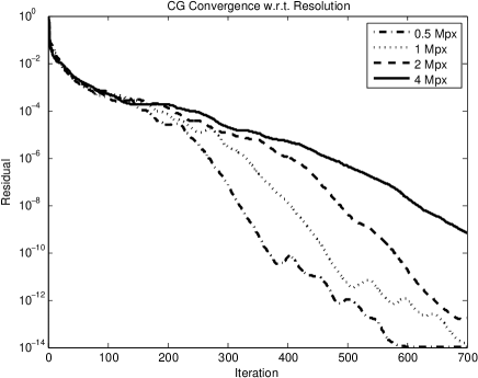
(a)

(b)

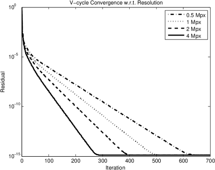
(c)

Figure 6: CG (a) & MGCG (b) slow down as resolution increases, while v-cycle (c) speeds up.

Resolution	CG	MGCG	v-cycle
0.5 Mpx	0.594	0.628	0.019
1 Mpx	0.357	0.430	0.017
2 Mpx	0.325	0.725	0.017
4 Mpx	0.314	0.385	0.015

TABLE I: Initial convergence rates $\rho_{0}$ on image 5 in [16]. Lower is better.

	CG			MGCG			v-cycle
Image	1 Mpx	2 Mpx	4 Mpx	1 Mpx	2 Mpx	4 Mpx	1 Mpx	2 Mpx	4 Mpx
1	143	159	179	81	81	94	12	11	11
2	151	176	185	73	86	99	12	10	10
3	215	280	334	103	108	118	12	9	8
4	345	439	542	143	171	230	16	14	11
5	180	211	236	44	120	95	13	12	10
6	126	148	180	65	91	61	11	10	9
7	152	179	215	86	84	96	11	10	8
8	314	385	468	135	167	180	16	12	9
9	237	285	315	87	119	91	12	11	8
10	122	149	180	72	72	95	10	9	8
11	171	192	78	77	96	32	12	11	7
12	127	151	179	65	86	77	9	8	7
13	266	291	317	143	156	159	18	15	11
14	125	145	175	76	79	83	13	12	11
15	129	156	190	67	69	105	12	12	11
16	292	374	468	123	171	178	15	14	12
17	153	190	230	63	81	86	10	8	7
18	183	238	289	86	104	107	26	22	16
19	91	104	116	52	58	61	12	10	8
20	137	164	199	81	82	101	12	9	7
21	195	288	263	118	83	137	22	16	15
22	118	139	161	62	75	72	11	9	7
23	140	166	196	64	77	74	11	9	8
24	213	266	325	76	131	104	14	14	10
25	319	455	629	142	170	249	39	31	24
26	370	432	478	167	192	229	41	32	24
27	271	304	349	121	144	147	17	15	12

TABLE II: Iterations to convergence (residual less than $10^{-4}$) at 1, 2, and 4 Mpx on images from [16]. CG and MGCG require more iterations as resolution increases while v-cycle requires less.

Image	$a$	$p$
1	11.8	-0.065
2	11.7	-0.140
3	11.8	-0.309
4	16.2	-0.261
5	13.2	-0.183
6	11.0	-0.144
7	11.2	-0.220
8	16.0	-0.415
9	12.3	-0.270
10	10.0	-0.160
11	12.5	-0.343
12	9.02	-0.180
13	18.2	-0.340
14	13.0	-0.120
15	12.2	-0.061
16	15.2	-0.156
17	9.90	-0.265
18	26.4	-0.333
19	12.1	-0.289
20	12.0	-0.394
21	21.4	-0.300
22	11.1	-0.321
23	10.9	-0.236
24	14.6	-0.216
25	39.1	-0.347
26	41.2	-0.381
27	17.2	-0.243

TABLE III: Fitting of v-cycle required iterations to $an^{p}$ (power law), with $n$ being problem size in Mpx. Average $p$ is $E[p]=-0.248$, meaning this solver is sublinear in $n$.

In order to compare the solution methods, we choose the matting Laplacian proposed by [4], as it is popular and provides source code. Please note that we are comparing the solvers, and not the performance of the matting Laplacian itself, as these solvers would equally apply to other matting Laplacians. We set their $\epsilon$ parameter to $10^{-3}$, and we form our linear system according to Eq. (5) with $\gamma=1$.

All methods are given the initial guess $\alpha_{0}=0$. To make the objective value comparable across methods and resolutions, we take $\left\lVert f-A\alpha_{i}\right\rVert_{2}/\left\lVert f-A\alpha_{0}\right\rVert_{2}=\left\lVert f-A\alpha_{i}\right\rVert_{2}/\left\lVert f\right\rVert_{2}$ as the normalized residual at iteration $i$, or residual for short. We set the termination condition for all methods at all resolutions to be the descent of the residual below $10^{-4}$.

First, we evaluate the convergence of conjugate gradient, multigrid conjugate gradient, and v-cycle. Typical behavior on the dataset [16] is shown in Fig. 5 at 4 Mpx resolution. CG takes many iterations to converge, MGCG performs somewhat better, and v-cycle performs best.

Next, we demonstrate in Fig. 6 that the number of iterations v-cycle requires to converge on the matting problem does not increase with the resolution. In fact, we discover that v-cycle requires fewer iterations as the resolution increases. This supports a sub-linear complexity of v-cycle on this problem in practice since each iteration is $\mathcal{O}\left(n\right)$.

We list a table of the convergence behavior of the algorithms on all images provided in the dataset in Table II. This demonstrates that MGCG performs decently better than CG, and that v-cycle always requires few iterations as the resolution increases. By fitting a power law to the required iterations in Table III, we find the average number of required v-cycle iterations is $\mathcal{O}\left(n^{-0.248}\right)$. Since each iteration is $\mathcal{O}\left(n\right)$, this means that this is the first solver demonstrated to have sublinear time complexity on the matting problem. Specifically, the time complexity is $\mathcal{O}\left(n^{0.752}\right)$ on average. Theoretical guarantees [14] ensure that the worst case time complexity is $\mathcal{O}\left(n\right)$.

Though surprising, the sub-linear behavior is quite understandable. Most objects to be matted are opaque with a boundary isomorphic to a line segment. The interior and exterior of the object have completely constant $\alpha$ locally, which is very easy for v-cycle to handle at its lower levels, since that is where the low frequency portions of the solution get solved. This leaves the boundary pixels get handled at the highest resolutions, since edges are high-frequency. These edge pixels contribute to the residual value, but since the ratio of boundary to non-boundary pixels is $\mathcal{O}\left(n^{-0.5}\right)$, tending to 0 with large $n$, the residual tends to decrease more rapidly per iteration as the resolution increases as proportiontely more of the problem gets solved in lower resolution.

Another way to view it is that there is a fixed amount of information present in the underlying image, and increasing the number of pixels past some point does not really add any additional information. V-cycle is simply the first algorithm studied to exploit this fact by focusing its effort preferentially on the low resolution parts of the solution.

Perhaps if we had enough computational resources and a high-enough resolution, v-cycle could drop the residual to machine epsilon in a single iteration. At that point, we would again have a linear complexity solver, as we would always have to do 1 iteration at $\mathcal{O}\left(n\right)$ cost. In any case, $\mathcal{O}\left(n\right)$ is worst case behavior as guaranteed by [14], which is still much better than any solver proposed to date like [5] and [6] (which are at best $\mathcal{O}\left(n^{2}\right)$). We would also like to mention that the per-iteration work done by the proposed method is constant with respect to the number of unknowns, unlike most solvers including [5] and [6].

Table I lists the initial convergence rates $\rho_{0}$ (the factor by which the residual is reduced per iteration). [14] guarantees that the convergence rate for v-cycle is at most $\mathcal{O}\left(1\right)$ and bounded away from 1. We discover that on the matting problem the convergence rate is sub-constant. Yet again, v-cycle dramatically overshadows other solvers.

Although a MATLAB implementation of [4] is available, we found it to use much more memory than we believe it should. We therefore developed our own implementation in C++ using efficient algorithms and data structures to run experiments at increasing resolution. Since there are 25 bands in the Laplacian, and 4 bytes per floating point entry, the storage required for the matrix in (5) is 95 MB/Mpx, and the total storage including the downsampled matrices is about 127 MB/Mpx. The time to generate the Laplacian is 0.8 s/Mpx. The CPU implementation runs at 46 Gauss-Seidel iterations/s/Mpx and 11 v-cycle iterations/s/Mpx. Assuming 10 iterations of v-cycle are run, which is reasonable from Table II, our solver runs in about 1.1 s/Mpx, which is nearly 5 times faster than [5] at low resolutions, and even faster at higher resolutions. Upon acceptance of this paper, we will post all the code under an open-source license.

Method	SAD	MSE	Gradient	Connectivity
Ours	11.1	10.8	12.9	9.1
[4]	14	13.9	14.5	6.4
[5]	17	15.8	16.2	9.2

TABLE IV: Average rank in benchmark [16] on 11 Mar 2013 with respect to different error metrics.

Although we consider this to be a matting solver rather than a new matting algorithm, we still submitted it to the online benchmark [16] using [4]’s Laplacian. The results presented in Table IV show some improvement over the base method [4], and more improvement over another fast method [5]. In theory, we should reach the exact same solution as [4] in this experiment, so we believe any performance gain is due to a different choice of their $\epsilon$ parameter.

5 Conclusion

We have thoroughly analyzed the performance of two multigrid algorithms, discovering that one exhibits sub-linear complexity on the matting problem. The $\mathcal{O}\left(n^{0.752}\right)$ average time complexity is by far the most efficient demonstrated to date. Further benefits of this approach include the ability to directly substitute any matting Laplacian of choice, and the capability to solve the original full-scale problem exactly without heuristics.

Appendix A Multigrid Algorithms

Algorithm 3 Multigrid gradient descent.

1:while  $numIter>0$  do

2:     $numIter\leftarrow numIter-1$

3:     $r_{\ell}\leftarrow b-Ax$

4:     $d_{\ell}\leftarrow r_{\ell}$

5:     for  $i=\ell-1..1$  do

6:         $r_{i}\leftarrow I_{i+1}^{i}r_{i+1}$

7:         $d_{i}\leftarrow r_{i}$

8:     end for

9:     for  $i=1..\ell$  do

10:         $k_{i}\leftarrow A_{i}d_{i}$

11:         for  $j=i..2$  do

12:              $k_{j-1}\leftarrow I_{j}^{j-1}k_{j}$

13:         end for

14:         $s_{1}=0$

15:         for  $j=1..i-1$  do

16:              $s_{j}\leftarrow s_{j}+(k_{j}^{T}d_{j})d_{j}$

17:              $s_{j+1}\leftarrow I_{j}^{j+1}s_{j}$

18:         end for

19:         $d_{i}\leftarrow d_{i}-s_{i}$

20:         $k_{i}\leftarrow A_{i}d_{i}$

21:         $d_{i}\leftarrow d_{i}(k_{i}^{T}d_{i})^{-\frac{1}{2}}$

22:     end for

23:     $s_{1}\leftarrow(d_{1}^{T}r_{1})d_{1}$

24:     for  $i=2..\ell$  do

25:         $s_{i}\leftarrow I_{i-1}^{i}s_{i-1}$

26:         $s_{i}\leftarrow s_{i}+d_{i}$

27:     end for

28:     $x\leftarrow x+s_{\ell}$

29:end while

Algorithm 4 Multigrid CG descent.

1:Do one iteration of multigrid gradient descent.

2:while  $numIter>0$  do

3:     $numIter\leftarrow numIter-1$

4:     $r_{\ell}\leftarrow b-Ax$

5:     $d_{\ell}^{\text{new}}\leftarrow r_{\ell}$

6:     for  $i=\ell-1..1$  do

7:         $r_{i}\leftarrow I_{i+1}^{i}r_{i+1}$

8:         $d_{i}^{\text{new}}\leftarrow r_{i}$

9:     end for

10:     for  $i=1..\ell$  do

11:         $k_{i}\leftarrow A_{i}d_{i}$

12:         for  $j=i..2$  do

13:              $k_{j-1}\leftarrow I_{j}^{j-1}k_{j}$

14:         end for

15:         $s_{1}=0$

16:         for  $j=1..i-1$  do

17:              $s_{j}\leftarrow s_{j}+(k_{j}^{T}d_{j}^{\text{new}})d_{j}^{\text{new}}$

18:              $s_{j+1}\leftarrow I_{j}^{j+1}s_{j}$

19:         end for

20:         $d_{i}\leftarrow d_{i}-s_{i}$

21:         $k_{i}\leftarrow A_{i}d_{i}$

22:         $d_{i}\leftarrow d_{i}(k_{i}^{T}d_{i})^{-\frac{1}{2}}$

23:         $k_{i}\leftarrow A_{i}d_{i}^{\text{new}}$

24:         for  $j=i..2$  do

25:              $k_{j-1}\leftarrow I_{j}^{j-1}k_{j}$

26:         end for

27:         $s_{1}\leftarrow 0$

28:         for  $j=1..i-1$  do

29:              $s_{j}\leftarrow s_{j}+d_{j}^{\text{new}}(k_{j}^{T}d_{j}^{\text{new}})$

30:              $s_{j}\leftarrow s_{j}+d_{j}(k_{j}^{T}d_{j}^{\text{new}})$

31:              $s_{j+1}\leftarrow I_{j}^{j+1}s_{j}$

32:         end for

33:         $d_{i}^{\text{new}}\leftarrow d_{i}^{\text{new}}-s_{i}$

34:         $s_{i}\leftarrow d_{i}^{\text{new}}-d_{i}(k_{i}^{T}d_{i})$

35:         if  $\left\lVert s_{i}\right\rVert_{\infty}>\epsilon\left\lVert d_{i}^{\text{new}}\right\rVert_{\infty}$  then

36:              $d_{i}^{\text{new}}\leftarrow s_{i}$

37:         else

38:              $d_{i}^{\text{new}}\leftarrow d_{i}$

39:              $d_{i}\leftarrow 0$

40:         end if

41:         $k_{i}\leftarrow A_{i}d_{i}^{\text{new}}$

42:         $d_{i}^{\text{new}}\leftarrow d_{i}^{\text{new}}(k_{i}^{T}d_{i}^{\text{new}})^{-1/2}$

43:     end for

44:     $d_{1}\leftarrow d_{1}^{\text{new}}$

45:     $s_{1}\leftarrow d_{1}(d_{1}^{T}r_{1})$

46:     for  $i=2..\ell$  do

47:         $d_{i}\leftarrow d_{i}^{\text{new}}$

48:         $s_{i}\leftarrow I_{i-1}^{i}s_{i-1}$

49:         $s_{i}\leftarrow s_{i}+d_{i}(d_{i}^{T}r_{i})$

50:     end for

51:     $x\leftarrow x+s_{\ell}$

52:end while

Philip Greggory Lee obtained his B.S. in Mathematics from Clemson University in 2008, where he published his first work in analytic number theory. He is currently pursuing a Ph.D. at Northwestern University in the Image and Video Processing Laboratory focusing on efficiency and scalability of computer vision algorithms. He is also involved with Northwestern’s Neuroscience & Robotics lab, working on high-speed vision systems for robotic manipulation.

Ying Wu received the B.S. from Huazhong University of Science and Technology, Wuhan, China, in 1994, the M.S. from Tsinghua University, Beijing, China, in 1997, and the Ph.D. in electrical and computer engineering from the University of Illinois at Urbana-Champaign (UIUC), Urbana, Illinois, in 2001. From 1997 to 2001, he was a research assistant at the Beckman Institute for Advanced Science and Technology at UIUC. During summer 1999 and 2000, he was a research intern with Microsoft Research, Redmond, Washington. In 2001, he joined the Department of Electrical and Computer Engineering at Northwestern University, Evanston, Illinois, as an assistant professor. He was promoted to associate professor in 2007 and full professor in 2012. He is currently full professor of Electrical Engineering and Computer Science at Northwestern University. His current research interests include computer vision, image and video analysis, pattern recognition, machine learning, multimedia data mining, and human-computer interaction. He serves as associate editors for IEEE Transactions on Pattern Aanlysis and Machine Intelligence, IEEE Transactions on Image Processing, IEEE Transactions on Circuits and Systems for Video Technology, SPIE Journal of Electronic Imaging, and IAPR Journal of Machine Vision and Applications. He received the Robert T. Chien Award at UIUC in 2001, and the NSF CAREER award in 2003. He is a senior member of the IEEE.

References

- [1] K. He, J. Sun, and X. Tang, “Single image haze removal using dark channel prior,” in Computer Vision and Pattern Recognition, 2009. CVPR 2009. IEEE Conference on. IEEE, 2009, pp. 1956–1963.
- [2] S. Dai and Y. Wu, “Motion from blur,” in Computer Vision and Pattern Recognition, 2008. CVPR 2008. IEEE Conference on. IEEE, 2008, pp. 1–8.
- [3] J. Fan, X. Shen, and Y. Wu, “Closed-loop adaptation for robust tracking,” in Computer Vision–ECCV 2010. Springer, 2010, pp. 411–424.
- [4] A. Levin, D. Lischinski, and Y. Weiss, “A closed-form solution to natural image matting,” IEEE Transactions on Pattern Analysis and Machine Intelligence, vol. 30, no. 2, pp. 228–242, 2008.
- [5] K. He, J. Sun, and X. Tang, “Fast matting using large kernel matting laplacian matrices,” in Computer Vision and Pattern Recognition (CVPR), 2010 IEEE Conference on. IEEE, 2010, pp. 2165–2172.
- [6] C. Xiao, M. Liu, D. Xiao, Z. Dong, and K.-L. Ma, “Fast closed-form matting using a hierarchical data structure,” Circuits and Systems for Video Technology, IEEE Transactions on, vol. 24, pp. 49–62, 2014.
- [7] R. Szeliski, “Locally adapted hierarchical basis preconditioning,” in ACM Transactions on Graphics (TOG), vol. 25, no. 3. ACM, 2006, pp. 1135–1143.
- [8] Y. Zheng and C. Kambhamettu, “Learning Based Digital Matting,” in ICCV, 2009.
- [9] P. G. Lee and Y. Wu, “Nonlocal matting,” in 2011 IEEE Conference on Computer Vision and Pattern Recognition. IEEE, 2011, pp. 2193–2200.
- [10] J. Sun, J. Jia, C.-K. Tang, and H.-Y. Shum, “Poisson matting,” in ACM Transactions on Graphics (ToG), vol. 23, no. 3. ACM, 2004, pp. 315–321.
- [11] O. Duchenne, J. Audibert, R. Keriven, J. Ponce, and F. Segonne, “Segmentation by transduction,” in IEEE Conference on Computer Vision and Pattern Recognition, 2008. CVPR 2008, 2008, pp. 1–8.
- [12] D. Singaraju, C. Rother, and C. Rhemann, “New appearance models for natural image matting,” 2009.
- [13] S. F. McCormick, Ed., Multigrid Methods. Society for Industrial and Applied Mathematics, 1987.
- [14] J. Gopalakrishnan and J. E. Pasciak, “Multigrid convergence for second order elliptic problems with smooth complex coefficients,” Computer Methods in Applied Mechanics and Engineering, vol. 197, no. 49, pp. 4411–4418, 2008.
- [15] C. Pflaum, “A multigrid conjugate gradient method,” Applied Numerical Mathematics, vol. 58, no. 12, pp. 1803–1817, 2008.
- [16] C. Rhemann, C. Rother, J. Wang, M. Gelautz, P. Kohli, and P. Rott, “A perceptually motivated online benchmark for image matting,” in Proc. CVPR. Citeseer, 2009, pp. 1826–1833.