Tensor completion in hierarchical tensor representations

Abstract

Compressed sensing extends from the recovery of sparse vectors from undersampled measurements via efficient algorithms to the recovery of matrices of low rank from incomplete information. Here we consider a further extension to the reconstruction of tensors of low multi-linear rank in recently introduced hierarchical tensor formats from a small number of measurements. Hierarchical tensors are a flexible generalization of the well-known Tucker representation, which have the advantage that the number of degrees of freedom of a low rank tensor does not scale exponentially with the order of the tensor. While corresponding tensor decompositions can be computed efficiently via successive applications of (matrix) singular value decompositions, some important properties of the singular value decomposition do not extend from the matrix to the tensor case. This results in major computational and theoretical difficulties in designing and analyzing algorithms for low rank tensor recovery. For instance, a canonical analogue of the tensor nuclear norm is NP-hard to compute in general, which is in stark contrast to the matrix case. In this book chapter we consider versions of iterative hard thresholding schemes adapted to hierarchical tensor formats. A variant builds on methods from Riemannian optimization and uses a retraction mapping from the tangent space of the manifold of low rank tensors back to this manifold. We provide first partial convergence results based on a tensor version of the restricted isometry property (TRIP) of the measurement map. Moreover, an estimate of the number of measurements is provided that ensures the TRIP of a given tensor rank with high probability for Gaussian measurement maps.

1 Introduction

As outlined in the introductory chapter of this book, compressed sensing allows the recovery of (approximately) sparse vectors from a small number of linear random measurements via efficient algorithms including $\ell_{1}$-minimization and iterative hard thresholding, see also rauhut ; elku12 for introductory material. This theory was later extended to the reconstruction of low rank matrices from random measurements in brecht ; cata10 ; capl11 ; gr11 . An important special case includes the matrix completion problem, where one seeks to fill in missing entries of a low rank matrix care09 ; cata10 ; gr11 ; re12 . Corresponding algorithms include nuclear norm minimization brecht ; cata10 ; fa02-2 and versions of iterative hard thresholding tanner .

In the present article we pursue a further extension of compressed sensing. We consider the recovery of a low rank tensor from a relatively small number of measurements. In contrast to already existing work in this direction recht ; goldfarb , we will understand low rank tensors in the framework of recently introduced hierarchical tensor formats hackbusch . This concept includes the classical Tucker format tucker ; kolda ; hosvd as well as tensor trains oseledets ; oseledets1 . These hierarchical tensors can be represented in a data sparse way, i.e., they require only a very low number of data for their representation compared to the dimension of the full tensor space.

Let us recall the setup of low rank matrix recovery first. Given a matrix $\mathbf{X}\in\mathbf{R}^{n_{1}\times n_{2}}$ of rank at most $r\ll\mbox{ min }\{n_{1},n_{2}\}$, the goal of low rank matrix recovery is to reconstruct $\mathbf{X}$ from linear measurements $b_{i}=1,\ldots,m$, i.e., $\mathbf{b}=\mathcal{A}(\mathbf{X})$, where $\mathcal{A}:\mathbb{R}^{n_{1}\times n_{2}}\to\mathbb{R}^{m}$ with $m\ll n_{1}n_{2}$ is a linear sensing operator.

This problem setting can be transferred to the problem to recover higher order tensors $\mathbf{u}\in\mathcal{H}_{d}:=\mathbb{R}^{n_{1}\times n_{2}\times\cdots\times n_{d}}$, $\boldsymbol{\mu}=(\mu_{1},\ldots,\mu_{d})\mapsto\mathbf{u}(\mu_{1},\ldots,\mu_{d})$ from the linear measurements $\mathbf{b}=\mathcal{A}(\mathbf{u})$, where $\mathcal{A}:\mathbb{R}^{n_{1}\times n_{2}\times\cdots\times n_{d}}\to\mathbb{R}^{m}$, is a sensing operator $m\ll n_{1}n_{2}\cdots n_{d}$. Here $d$ denotes the order of the tensor (number of modes of a tensor) and we remark that, for easier readability, we use the notation $\mathbf{u}(\mu_{1},\ldots,\mu_{d})$ referring to the entries of the tensor. In the present article we assume that the tensors to be reconstructed belong to a class of hierarchical tensors of a given low multi-linear rank $\mathbf{r}=(r_{j})_{j=1}^{p}$, where $p$ depends on the specific tensor format dasilva , see also below. Of particular interest is the special case of tensor completion, where the measurement operator samples entries of the tensor, i.e.,

$$\big{(}\mathcal{A}\mathbf{u}\big{)}_{i}=\mathbf{u}({\boldsymbol{\mu}_{i}})=\mathbf{u}(\mu_{1,i},\ldots,\mu_{d,i})=b_{i}\ \ ,\ \ i=1,\ldots,m\ ,$$

where the $\boldsymbol{\mu}_{i}\in\Omega$, $|\Omega|=m$, are given (multi-)indices mohlenkamp ; signoretto1 ; kressner . Tensors, even of high order $d\gg 3$, appear frequently in data and signal analysis. For example, a video signal is a tensor of order $d=3$. High order tensors of relatively low rank may also arise in vector-tensorization hackbusch-tensorisation ; oseledets-qtt of a low dimensional signal. The present article tries to present a framework for tensor recovery from the perspective of recent developments in tensor product approximation kolda ; belmol ; hackbusch , in particular the development of hierarchical tensors hackbusch ; oseledets . The canonical format (CANDECOMP, PARAFAC) representing a tensor of order $d$ as a sum of elementary tensor products, or rank one tensors (see kolda ; belmol )

$$\mathbf{u}(\mu_{1},\ldots,\mu_{d}) = \sum_{k=1}^{r}\big{(}\mathbf{c}^{1}_{k}\otimes\cdots\otimes\mathbf{c}^{d}_{k}\big{)}(\mu_{1},\ldots,\mu_{d})$$

$$= \sum_{k=1}^{r}\mathbf{c}^{1}_{k}(\mu_{1})\cdots\mathbf{c}^{d}_{k}(\mu_{d})\ \ ,\ \ \mu_{i}=1,\ldots,n_{i}\ ,\ i=1,\ldots,d\ ,$$

with $\mathbf{c}^{i}_{k}\in\mathbb{R}^{n_{i}}$, suffers from severe difficulties, unless $d\leq 2$. For example, the tensor rank is not well defined, and the set of tensors of the above form with fixed $r$ is not closed lim and does not form an algebraic variety. However, we obtain a closed subset, if we impose further conditions. Typical examples for such conditions are e.g. symmetry landsberg or bounds $\left|\mathbf{c}_{k}^{i}\right|\leq\alpha$ for some fixed $\alpha$ usch .

However, it has been experienced that computations within the Tucker tensor format behave relatively robust and stable, whereas the complexity unfortunately still suffers from the curse of dimensionality. A first important observation may be summarized in the fact that the set of Tucker tensors with a Tucker rank at most $\mathbf{r}=(r_{1},\ldots,r_{d})$ forms an algebraic variety, i.e., a set of common zeros of multi-variate polynomials. Recently developed hierarchical tensors, introduced by Hackbusch and coworkers (HT tensors) hackbusch-kuehn ; lars and the group of Tyrtyshnikov (tensor trains, TT) oseledets ; oseledets1 have extended the Tucker format tucker ; kolda ; hosvd into a multi-level framework, that no longer suffers from high order scaling w.r.t. the order $d$, as long as the ranks are moderate. For $d=3$ there is no essential difference, whereas for larger $d\geq 4$ one benefits from the use of the novel formats. This makes the Tucker format signoretto1 ; goldfarb ; yin and, in particular, its hierarchical generalization dasilva ; kressner ; rss1 , the hierarchical tensor format, a proper candidate for tensor product approximation in the sense that it serves as an appropriate model class in which we would like to represent or approximate tensors of interest in a data sparse way. Several algorithms developed in compressed sensing and matrix recovery or matrix completion can be easily transferred to this tensor setting (with the exception of nuclear norm minimization, which poses some fundamental difficulties). However, we already note at this point that the analysis of algorithms is much harder for tensors than for matrices as we will see below.

Historically, the hierarchical tensor framework has evolved in the quantum physics community hidden in the renormalization group ideas white , and became clearly visible in the framework of matrix product and tensor network states schollwoeck . An independent source of these developments can be found in quantum dynamics as the multi-layer multiconfigurational time-dependent Hartree (MCTDH) method mayer ; wang ; lubich-blau . Only after the recent introduction of hierarchical tensor representations in numerics, namely Hierarchical Tucker (HT) hackbusch ; hackbusch-kuehn and Tensor Trains (TT) oseledets ; oseledets1 , its relationship to already existing concepts in quantum physics has been realized lrss . We refer the interested reader to the recent survey articles hackbuschAN ; grasedyck-kressner ; lrss ; hs and the monograph hackbusch . In the present paper we would like to provide a fairly self-contained introduction, and demonstrate how these concepts can be applied for tensor recovery.

There are several essential difficulties when passing from matrix to tensor recovery. In matrix recovery, the original problem can be reformulated to finding the solution of the optimization problem

$$\mbox{minimize rank}({\bf Z})\mbox{ s.t. }\mathcal{A}({\bf Z})={\bf b}\ ,\ {\bf Z}\in\mathbb{R}^{n_{1}\times n_{2}},$$

i.e., to finding the matrix $\mathbf{Z}$ with the lowest rank consistent with the measurements. While this problem is NP-hard fa02-2 , it can be relaxed to the convex optimization problem of constrained nuclear norm minimization

$$\mbox{ minimize }\|{\bf Z}\|_{*}\mbox{ s.t. }\mathcal{A}({\bf Z})={\bf b}\ ,\ {\bf Z}\in\mathbb{R}^{n_{1}\times n_{2}}\ .$$

Here, the nuclear norm is the sum of the singular values $\sigma_{j}({\bf Z})$ of ${\bf Z}$, i.e., $\|{\bf Z}\|_{*}=\sum_{j}\sigma_{j}({\bf Z})$. The minimizer of this problem reconstructs ${\bf X}$ exactly under suitable conditions on $\mathcal{A}$ brecht ; capl11 ; care09 ; gr11 ; rauhut .

In the hierarchical tensor setting, we are dealing with a rank tuple $\mathbf{r}=(r_{1},\ldots,r_{p})$, which we would like to minimize simultaneously. However, this is not the only difficulty arising from the non-linear tensor ansatz. In fact, the tensor nuclear norm is NP-hard to compute NPcomplete ; Fried and therefore, tensor nuclear norm minimization is computationally prohibitive. Another difficulty arises because in contrast to the matrix case, also the best rank ${\mathbf{r}}$-approximation to a given tensor is NP-hard to compute NPcomplete ; Fried .

Our model class of hierarchical tensors of fixed multi-linear rank $\mathbf{r}$ is a smooth embedded manifold, and its closure constitutes an algebraic variety. These are properties on which one can built local optimization methods absil ; lrsv ; su2 , subsumed under the moniker Riemannian optimization. Moreover, for hierarchical tensor representation efficient numerical tools for finding at least a quasi-best approximation are available, namely the higher order singular value decomposition (HOSVD), related to the Tucker model hosvd , or the hierarchical singular value decomposition (HSVD), which is an extension of the HOSVD to hierarchical Tucker models oseledets2 ; hackbusch ; lars ; vidal . All these methods proceed via successive computations of the SVD of certain matricisations of the original tensor.

The HSVD (and the HOSVD as a special case) enables us to compute rank ${\mathbf{r}}$ approximations to a given tensor via truncation of the decomposition. This allows to extend a particular class of greedy type algorithms, namely iterative hard thresholding algorithms to the present tensor setting. In a wider sense, this class of techniques includes also related Riemannian manifold techniques kressner ; dasilva and alternating least squares methods hrs-als . First numerical tests show promising results dasilva ; kressner ; rss1 ; rss2 . For a convergence analysis in the tensor case, and in applications, however, we have to struggle with more and harder difficulties than in the matrix case. The most fundamental of these consists in the fact, that truncations of the HSVD only provide quasi-best low rank approximations. Although bounds of the approximation error are known lars , they are not good enough for our purposes, which is the main reason why we are only able to provide partial convergence results in this chapter. Another difficulty with iterative hard thresholding algorithms is that the rank, here a rank tuple $\mathbf{r}=(r_{1},\ldots,r_{p})$, has to be fixed a priori. In practice this rank tuple is not known in advance, and a strategy for specifying appropriate ranks is required. Well known strategies borrowed from matrix recovery consist in increasing the rank during the approximation or starting with overestimating the rank and reduce the ranks through the iteration wutao . For our seminal treatment, we simply assume that the multi-linear rank $\mathbf{r}$ is known in advance, i.e., the sought tensor $\mathbf{u}$ is of exact rank $\mathbf{r}$. Moreover, we assume noiseless measurements $\big{(}\mathcal{A}\mathbf{u}\big{)}_{j}=b_{j}\in\mathbb{R}$, $j=1,\ldots,m$. The important issues of adapting ranks and obtaining robustness will be deferred to future research rss2 .

Our chapter is related to the one on two algorithms for compressed sensing of sparse tensors by S. Friedland, Q. Li, D. Schonfeld and E.E. Bernal. The latter chapter also considers the recovery of mode $d$-tensors from incomplete information using efficient algorithms. However, in contrast to our chapter, the authors assume usual sparsity of the tensor instead of the tensor being of low rank. The tensor structure is used in order to simplify the measurement process and to speed up the reconstruction rather than to work with the smallest possible number of measurements and to exploit low-rankness.

2 Hierarchical Tensors

2.1 Tensor product spaces

We start with some preliminaries. In the sequel, we consider only the real field $\mathbb{K}=\mathbb{R}$, but most parts are easy to extend to the complex case as well. We will confine ourselves to finite dimensional linear spaces $V_{i}=\mathbb{R}^{n_{i}}$ from which the tensor product space

$$\mathcal{H}_{d}=\bigotimes_{i=1}^{d}V_{i}:=\bigotimes_{i=1}^{d}\mathbb{R}^{n_{i}}\ \ ,$$

is built hackbusch . If it is not stated explicitly, the $V_{i}=\mathbb{R}^{n_{i}}$ are supplied with the canonical basis $\{\mathbf{e}^{i}_{1},\ldots,\mathbf{e}^{i}_{n_{i}}\}$ of the vector space $\mathbb{R}^{n_{i}}$. Then any $\mathbf{u}\in\mathcal{H}_{d}$ can be represented as

$$\mathbf{u} = \sum_{\mu_{1}=1}^{n_{1}}\ldots\sum_{\mu_{d}=1}^{n_{d}}\mathbf{u}(\mu_{1},\ldots,\mu_{d})\;\mathbf{e}^{1}_{\mu_{1}}\otimes\cdots\otimes\mathbf{e}^{d}_{\mu_{d}}\ .$$

Using this basis, with a slight abuse of notation, we can identify $\mathbf{u}\in\mathcal{H}_{d}$ with its representation by a d-variate function, often called hyper matrix,

$$\boldsymbol{\mu}=(\mu_{1},\ldots,\mu_{d})\mapsto\mathbf{u}(\mu_{1},\ldots,\mu_{d})\in\mathbb{R}\ \ ,\ \ \mu_{i}=1,\ldots,n_{i}\ ,\ i=1,\ldots,d\ ,$$

depending on discrete variables, usually called indices $\mu_{i}=1,\ldots,n_{i}$, and $\boldsymbol{\mu}$ is called a multi-index. Of course, the actual representation $\mathbf{u}(\cdots)$ of $\mathbf{u}\in\mathcal{H}_{d}$ depends on the chosen bases of $V_{1},\ldots,V_{d}$. With $n=\max\{n_{i}:i=1,\ldots,d\}$, the number of possibly non-zero entries in the representation of $\mathbf{u}$ is $n_{1}\cdots n_{d}=\mathcal{O}(n^{d})$. This is often referred to as the curse of dimensions. We equip the linear space $\mathcal{H}_{d}$ with the $\ell_{2}$-norm $\|\mathbf{u}\|=\sqrt{\langle\mathbf{u},\mathbf{u}\rangle}$ and the inner product

$$\langle\mathbf{u},\mathbf{v}\rangle:=\sum_{\mu_{1}=1}^{n_{1}}\cdots\sum_{\mu_{d}=1}^{n_{d}}{\mathbf{u}(\mu_{1},\ldots,\mu_{d})}\mathbf{v}(\mu_{1},\ldots,\mu_{d})\ .$$

We distinguish linear operators between vector spaces and their corresponding representation by matrices, which are written by capital bold letters $\mathbf{U}$. Throughout this chapter, all tensor contractions or various tensor–tensor products are either defined explicitly, by summation over corresponding indices, or by introducing corresponding matricisations of the tensors and performing matrix–matrix products.

2.2 Subspace approximation

The essence of the classical Tucker format is that, given a tensor $\mathbf{u}$ and a rank-tuple $\mathbf{r}=(r_{j})_{j=1}^{d}$, one is searching for optimal subspaces $U_{i}\subset\mathbb{R}^{n_{i}}$ such that

$$\min\|\mathbf{u}-\mathbf{v}\|,\mbox{ where }\mathbf{v}\in U_{1}\otimes\cdots\otimes U_{d},$$

is minimized over $U_{1},\ldots,U_{d}$ with $\dim U_{i}=r_{i}$. Equivalently, we are looking for corresponding bases $\mathbf{b}^{i}_{k_{i}}$ of $U_{i}$, which can be written in the form

$$\mathbf{b}^{i}_{k_{i}}:=\sum_{\mu_{i}=1}^{n_{i}}\mathbf{b}^{i}(\mu_{i},k_{i})\mathbf{e}^{i}_{\mu_{i}}\ \ ,\ \ \ k_{i}=1,\ldots,r_{i}<n_{i}\ ,$$ (2)

where $\mathbf{b}^{i}(k_{i},\mu_{i})\in\mathbb{R}$, for each coordinate direction $i=1,\ldots,d$. With a slight abuse of notation we often identify the basis vector with its representation

$$\mathbf{b}^{i}_{k_{i}}\simeq\big{(}\mu_{i}\mapsto\mathbf{b}^{i}(\mu_{i},k_{i})\big{)}\ ,\ \mu_{i}=1,\ldots,n_{i}\ ,\ \ k_{i}=1,\ldots,r_{i}\ ,$$

i.e., a discrete function or an $n_{i}$-tuple. This concept of subspace approximation can be used either for an approximation $\mathbf{u}$ of a single tensor, as well as for an ensemble of tensors $\mathbf{u}_{j}$, $j=1,\dots,m$, in tensor product spaces. Given the bases $\mathbf{b}^{i}_{k_{i}}$, $\mathbf{u}_{j}$ can be represented by

$$\mathbf{u}_{j}=\sum_{k_{1}=1}^{r_{1}}\ldots\sum_{k_{d}=1}^{r_{d}}\mathbf{c}(j,k_{1},\ldots,k_{d}){\bf b}^{1}_{k_{1}}\otimes\cdots\otimes{\bf b}^{d}_{k_{d}}\in\bigotimes_{i=1}^{d}U_{i}\subset\mathcal{H}_{d}=\bigotimes_{i=1}^{d}{\mathbb{R}}^{n_{i}}\ .$$ (3)

In case $\mathbf{b}^{i}$’s form orthonormal bases, the core tensor $\mathbf{c}\in\mathbb{R}^{m}\otimes\bigotimes_{i=1}^{d}\mathbb{R}^{r_{i}}$ is given entry-wise by

$$\mathbf{c}(j,k_{1},\ldots,k_{d})=\langle\mathbf{u}_{j},\mathbf{b}^{1}_{k_{1}}\otimes\cdots\otimes\mathbf{b}^{d}_{k_{d}}\rangle\ .$$

We call a representation of the form (3) with some $\mathbf{b}_{k_{i}}^{i},\mathbf{c}$ a Tucker representation, and the Tucker representations the Tucker format. In this formal parametrization, the upper limit of the sums may be larger than the ranks and $\{\mathbf{b}_{k_{i}}^{i}\}_{k_{i}}$ may not be linearly independent. Noticing that a Tucker representation of a tensor is not uniquely defined, we are interested in some normal form.

Since the core tensor contains $r_{1}\cdots r_{d}\sim r^{d}$, $r:=\max\{r_{i}:i=1,\ldots,d\}$, possibly nonzero entries, this concept does not prevent the number of free parameters from scaling exponentially with the dimensions $\mathcal{O}(r^{d})$. Setting $n:=\max\{n_{i}:i=1,\ldots,d\}$, the overall complexity for storing the required data (including the basis vectors) is bounded by $\mathcal{O}(ndr+r^{d})$. Since $n_{i}$ is replaced by $r_{i}$, one obtains a dramatical compression $\frac{r_{1}}{n_{1}}\cdots\frac{r_{d}}{n_{d}}\sim\big{(}\frac{r}{n}\big{)}^{d}$. Without further sparsity of the core tensors the Tucker format is appropriate for low order tensors $d<4$.

2.3 Hierarchical tensor representation

The hierarchical Tucker format (HT) in the form introduced by Hackbusch and Kühn in hackbusch-kuehn , extends the idea of subspace approximation to a hierarchical or multi-level framework. Let us proceed in a hierarchical way. We first consider $V_{1}\otimes V_{2}=\mathbb{R}^{n_{1}}\otimes\mathbb{R}^{n_{2}}$ or preferably the subspaces $U_{1}\otimes U_{2}$ introduced in the previous section. For the approximation of $\mathbf{u}\in\mathcal{H}_{d}$ we only need a subspace $U_{\{1,2\}}\subset U_{1}\otimes U_{2}$ with dimension $r_{\{1,2\}}<r_{1}r_{2}$. Indeed, $V_{\{1,2\}}$ is defined through a new basis

$$V_{\{1,2\}} = \mbox{span }\{\mathbf{b}^{\{1,2\}}_{k_{\{1,2\}}}:k_{\{1,2\}}=1,\ldots,r_{\{1,2\}}\}\ ,$$

with basis vectors given by

$$\mathbf{b}^{\{1,2\}}_{k_{\{1,2\}}}=\sum_{{k}_{1}=1}^{r_{1}}\sum_{{k}_{2}=1}^{r_{2}}\mathbf{b}^{\{1,2\}}(k_{1},k_{2},k_{\{1,2\}})\;{\bf b}^{1}_{k_{1}}\otimes{\bf b}^{2}_{k_{2}},\quad k_{\{1,2\}}=1,\ldots,r_{\{1,2\}}.$$

One may continue in several ways, e.g. by building a subspace $U_{\{1,2,3\}}\subset U_{\{1,2\}}\otimes U_{3}\subset U_{1}\otimes U_{2}\otimes U_{3}\subset V_{1}\otimes V_{2}\otimes V_{3}$, or $U_{\{1,2,3,4\}}\subset U_{\{1,2\}}\otimes U_{\{3,4\}}$, where $U_{\{3,4\}}$ is defined analogously to $U_{\{1,2\}}$ and so on.

For a systematic treatment, this approach can be cast into the framework of a partition tree, with leaves $\{1\},\ldots\{d\}$, simply abbreviated here by $1,\ldots,d$, and vertices $\alpha\subset D:=\{1,\ldots,d\}$, corresponding to the partition $\alpha=\alpha_{1}\cup\alpha_{2}$ , $\alpha_{1}\cap\alpha_{2}=\emptyset$. Without loss of generality, we can assume that $i<j$, for all $i\in\alpha_{1}$, $j\in\alpha_{2}$. We call $\alpha_{1},\alpha_{2}$ the sons of the father $\alpha$ and $D$ is called the root of the tree. In the example above we have $\alpha:=\{1,2,3\}=\alpha_{1}\cup\alpha_{2}=\{1,2\}\cup\{3\}$, where $\alpha_{1}:=\{1,2\}$ and $\alpha_{2}:=\{3\}$.

In general, we do not need to restrict the number of sons, and define the coordination number by the number of sons $+1$ (for the father). Restricting to a binary tree so that each node contains two sons for non-leaf nodes (i.e. $\alpha\not=\{i\}$), is often the common choice, which we will also consider here. Let $\alpha_{1},\alpha_{2}\subset D$ be the two sons of $\alpha\subset D$, then $U_{\alpha}\subset U_{\alpha_{1}}\otimes U_{\alpha_{2}}$, is defined by a basis

$$\mathbf{b}^{\alpha}_{\ell}=\sum_{i=1}^{r_{\alpha_{1}}}\sum_{j=1}^{r_{\alpha_{2}}}\mathbf{b}^{\alpha}(i,j,\ell)\mathbf{b}^{\alpha_{1}}_{i}\otimes\mathbf{b}^{\alpha_{2}}_{j}\ .$$ (4)

They can also be considered as matrices $(\mu_{\alpha},\ell)\mapsto\mathbf{B}^{\alpha}(\mu_{\alpha},\ell)\in\mathbb{R}^{n_{\alpha}\times r_{\alpha}}$ with $n_{\alpha}=\prod_{\ell\in\alpha}n_{\ell}$, for $\alpha\neq\{i\}$. Without loss of generality, all basis vectors, e.g. $\{\mathbf{b}^{\alpha}_{\ell}:\ell=1,\ldots,r_{\alpha}\}$, can be constructed to be orthonormal, as long as $\alpha\not=D$ is not the root. The tensors $(\ell,i,j)\mapsto\mathbf{b}^{\alpha}(i,j,\ell)$ will be called transfer or component tensors. For a leaf $\{i\}\simeq i$, the tensor $(\mu_{i},k_{i})\mapsto\mathbf{b}^{i}(\mu_{i},k_{i})$ in (2) denotes a transfer or component tensor. The component tensor $\mathbf{b}^{D}=\mathbf{b}^{\{1,\ldots,d\}}$ at the root is called the root tensor.

Since the matrices $\mathbf{B}^{\alpha}$ are too large, we avoid computing them. We store only the transfer or component tensors which, for fixed $\ell=1,\ldots,r_{\alpha}$, can also be casted into transfer matrices $(i,j)\mapsto\mathbf{B}_{\alpha}(\ell)_{i,j}\in\mathbb{R}^{r_{\alpha_{1}}\times r_{\alpha_{2}}}$.

Proposition 1 (hackbusch )

A tensor $\mathbf{u}\in\mathcal{H}_{d}$ is completely parametrized by the transfer tensors $\mathbf{b}^{\alpha}$, $\alpha\in\mathbb{T}$, i.e., by a multi-linear function $\tau$

$$\big{(}\mathbf{b}^{\alpha}\big{)}_{\alpha\in\mathbb{T}}\mapsto\mathbf{u}=\tau\big{(}\{\mathbf{b}^{\alpha}:\alpha\in\mathbb{T}\}\big{)}\ .$$

Indeed $\tau$ is defined by applying (4) recursively. Since $\mathbf{b}^{\alpha}$ depends bi-linearly on $\mathbf{b}^{\alpha_{1}}$ and $\mathbf{b}^{\alpha_{2}}$, the composite function $\tau$ is multi-linear in its arguments $\mathbf{b}^{\alpha}$.

Hierarchical Tensor representation of an order $5$ tensor

Data complexity Let $n:=\max\{n_{i}:i=1,\ldots,d\}$, $r:=\max\{r_{\alpha}:\alpha\in\mathbb{T}\}$. Then the number of data required for the representation is $\mathcal{O}(ndr+dr^{3})$, in particular does not scale exponentially w.r.t. the order $d$.

2.4 Tensor trains and matrix product representation

We now highlight another particular case of hierarchical tensor representations, namely Tyrtyshnikov tensors (TT) or tensor trains and matrix product representations defined by taking $U_{\{1,\ldots,p+1\}}\subset U_{\{1,\ldots,p\}}\otimes V_{\{p+1\}}$, developed as TT tensors (tensor trains) by oseledets1 ; oseledets2 and known as matrix product states (MPS) in physics. Therein, we abbreviate $i\simeq\{1,\ldots,i\}$ and consider the unbalanced tree $\mathbb{T}=\{\{1\},\{2\},\{1,2\},\{3\},\{1,2,3\},\ldots,\{d\},\{1,\ldots,d\}\}$ and setting $r_{0}=r_{d}=1$. The transfer tensor $\mathbf{b}^{\alpha}$ for a leaf $\alpha\in\{\{2\},\{3\},\ldots,\{d\}\}$ is usually defined as identity matrix of appropriate size and therefore the tensor $\mathbf{u}\in\mathcal{H}_{d}$ is completely parametrized by transfer tensors $\left(\mathbf{b}^{\alpha}\right)_{\alpha\in\mathbb{T}^{\prime}}$, where $\mathbb{T}^{\prime}=\{1,\ldots,d\}=\{\{1\},\{1,2\},\ldots$, $\{1,2,\ldots,d\}\}$. Applying the recursive construction, the tensor $\mathbf{u}$ can be written as

$$(\mu_{1},\ldots,\mu_{d}) \mapsto \mathbf{u}(\mu_{1},\ldots,\mu_{d})$$ (5)

$$= \sum_{k_{1}=1}^{r_{1}}\ldots\sum_{k_{d-1}=1}^{r_{d-1}}{\mathbf{b}^{1}(\mu_{1},k_{1})\mathbf{b}^{2}(k_{1},\mu_{2},k_{2})\cdots\mathbf{b}^{d}(k_{d-1},\mu_{d})}\ .$$

Introducing the matrices $\mathbf{B}_{i}(\mu_{i})\in\mathbb{R}^{r_{i-1}\times r_{i}}$,

$$\big{(}\mathbf{B}_{i}(\mu_{i})\big{)}_{k_{i-1},k_{i}}=\mathbf{b}^{i}(k_{i-1},\mu_{i},k_{i})\ ,\ 1\leq i\leq d\ ,$$

and with the convention $r_{0}=r_{d}=1$

$$\big{(}\mathbf{B}_{1}(\mu_{1})\big{)}_{k_{1}}^{*}=\mathbf{b}^{1}(\mu_{1},k_{1})\ \ \text{and}\ \ \big{(}\mathbf{B}_{d}(\mu_{d})\big{)}_{k_{d-1}}=\mathbf{b}^{d}(k_{d-1},\mu_{d})\ ,$$

the formula (5) can be rewritten entry-wise by matrix–matrix products

$$\mathbf{u}(\mu_{1},\ldots,\mu_{d})={\mathbf{B}_{1}(\mu_{1})\cdots\mathbf{B}_{i}(\mu_{i})\cdots\mathbf{B}_{d}(\mu_{d})}=\tau(\mathbf{b}^{1},\ldots,\mathbf{b}^{d})\ .$$ (6)

This representation is by no means unique. In general, there exist $\mathbf{b}^{\alpha}\neq\mathbf{c}^{\alpha}$ such that $\tau(\{\mathbf{b}^{\alpha}:\alpha\in\mathbb{T}\})=\tau(\{{\mathbf{c}}^{\alpha}:\alpha\in\mathbb{T}\})$.

TT representation of an order $5$ tensor with abbreviation $i\simeq\{1,\ldots,i\}$

The tree is ordered according to the father-son relation into a hierarchy of levels, where $\mathbf{b}^{d}$ is the root tensor. Let us observe that we can rearrange the hierarchy in such a way that any node $p=1,\ldots,{d}$ can form the root of the tree, i.e., $\mathbf{b}^{p}$ becomes the root tensor. Using only orthogonal basis vectors, which is the preferred choice, this ordering reflects left and right hand orthogonalization in matrix product states hrs-tt .

A tensor in canonical form

$$\mathbf{u}=\sum_{k=1}^{R}\mathbf{u}_{k}^{1}\otimes\cdots\otimes\mathbf{u}_{k}^{d}$$

can be easily written in the TT form, by setting $r_{i}=R$, for all $i=1,\ldots,d-1$ and

$$\mathbf{b}^{i}(k_{i-1},\mu_{i},k_{i})=\begin{cases}\begin{array}[]{cl}\mathbf{u}^{i}_{k}(\mu_{i})&\mbox{if }k_{i-1}=k_{i}=k,\,i=2,\ldots,d-1\\ 0&\mbox{if }k_{i-1}\not=k_{i},\,i=2,\ldots,d-1\\ \mathbf{u}^{i}_{k}(\mu_{i})&\mbox{if }k_{i}=k,\,i=1\\ \mathbf{u}^{i}_{k}(\mu_{i})&\mbox{if }k_{i-1}=k,\,i=d\end{array}\end{cases}\ .$$

Data complexity: Let $n:=\max\{n_{i}:i=1,\ldots,d\}$, $r:=\max\{r_{j}:j=1,\ldots,d-1\}$. Then the number of data required for the presentation is $\mathcal{O}(dnr^{2})$. Computing a single entry of a tensor requires the matrix multiplication of $d$ matrices of size at most $r\times r$. This can be performed in $\mathcal{O}(ndr^{3})$ operations.

Since the parametrization $\tau$ can be written in the simple matrix product form (6), we will consider the TT format often as a prototype model, and use it frequently for our explanations. We remark that most properties can easily be extended to the general hierarchical case with straightforward modifications hackbusch , and we leave those modifications to the interested reader.

2.5 Matricisation of a tensor and its multi-linear rank

Let $\mathbf{u}$ be a tensor in $\mathcal{H}_{d}$. Given a fixed dimension tree $\mathbb{T}$, for each node $\alpha\in\mathbb{T}$, $\alpha\not=D$, we can build a matrix $\mathbf{U}^{\alpha}$ from $\mathbf{u}$ by grouping the indices $\mu_{i}$, with $i\in\alpha$ into a row index $I$ and the remaining indices $\mu_{j}$ with $j\in D\backslash\alpha$ into the column index $J$ of the matrix $\mathbf{U}^{\alpha}=\big{(}\mathbf{U}^{\alpha}_{I,J}\big{)}$. For the root $\alpha=D$ we simply take the vectorized tensor $\mathbf{U}^{D}\in\mathbb{R}^{n_{1}\cdots n_{d}\times 1}$. Since the rank of this matrix is one, it is often omitted.

For example, in the Tucker case, for $\alpha=\{i\}$ being a leaf, we set $I=\mu_{i}$ and $J=(\mu_{1},\ldots,\mu_{i-1},\mu_{i+1},\ldots,\mu_{d})$ providing a matrix

$$\mathbf{U}^{\alpha}_{\mu_{i};(\mu_{1},\ldots,\mu_{i-1},\mu_{i+1},\ldots,\mu_{d})}=\mathbf{u}(\mu_{1},\ldots,\mu_{d})\ .$$

Similar, in the TT-format, with the convention that $i\simeq\{1,\ldots,i\}$, we obtain matrices $\mathbf{U}^{i}\in\mathbb{R}^{n_{1}\cdots n_{i}\times n_{i+1}\cdots n_{d}}$ with entries

$$\mathbf{U}^{i}_{(\mu_{1},\ldots,\mu_{i});(\mu_{i+1},\ldots,\mu_{d})}=\mathbf{u}(\mu_{1},\ldots,\mu_{d})\ .$$

Definition 1

Given a dimension tree $\mathbb{T}$ with $p$ nodes, we define the multi-linear rank by the $p$-tuple $\mathbf{r}=(r_{\alpha})_{\alpha\in\mathbb{T}}$ with $r_{\alpha}=\operatorname{rank}(\mathbf{U}^{\alpha})$, $\alpha\in\mathbb{T}$. The set of tensors $\mathbf{u}\in\mathcal{H}_{d}$ of given multi-linear rank $\mathbf{r}$ will be denoted by $\mathcal{M}_{\mathbf{r}}$. The set of all tensors of rank $\mathbf{s}$ at most $\mathbf{r}$, i.e., $s_{\alpha}\leq r_{\alpha}$ for all $\alpha\in\mathbb{T}$ will be denoted by $\mathcal{M}_{\leq\mathbf{r}}$.

Unlike the matrix case, it is possible that for some tuples $\mathbf{r}$, $\mathcal{M}_{\mathbf{r}}=\emptyset$ Carlini . However, since our algorithm works on a closed nonempty set $\mathcal{M}_{\leq\mathbf{r}}$, this issue does not concern us.

In contrast to the canonical format (1), also known as CANDECOMP/PARAFAC, see LimSilva ; kolda and the border rank problem landsberg , in the present setting the rank is a well defined quantity. This fact makes the present concept highly attractive for tensor recovery. On the other hand, if a tensor $\mathbf{u}$ is of rank $\mathbf{r}$ then there exists a component tensor $\mathbf{b}^{\alpha}$ of the form (4) where $\ell=1,\ldots,r_{\alpha}$.

It is well known that the set of all matrices $\mathbf{A}\in\mathbb{R}^{n\times m}$ of rank at most $r$ is a set of common zeros of multi-variate polynomials, i.e., an algebraic variety. The set $\mathcal{M}_{\leq\mathbf{r}}$ is the set of all tensors $\mathbf{u}\in\mathcal{H}_{d}$, where the matrices $\mathbf{U}^{\alpha}$ have a rank at most $r_{\alpha}$. Therefore, it is again a set of common zeros of multivariate polynomials.

2.6 Higher order singular value decomposition

Let us provide more details about the rather classical higher order singular value decomposition. Above we have considered only binary dimension trees $\mathbb{T}$, but we can extend the considerations also to $N$-ary trees with $N\geq 3$. The $d$-ary tree $\mathbb{T}$ (the tree with a root with $d$ sons $i\simeq\{i\}$) induces the so-called Tucker decomposition and the corresponding higher order singular value decomposition (HOSVD). The Tucker decomposition was first introduced by Tucker in $1963$ Tucker and has been refined later on in many works, see e.g. levin ; Tucker2 ; Tucker .

Definition 2 (Tucker decomposition)

Given a tensor $\mathbf{u}\in\mathbb{R}^{n_{1}\times\cdots\times n_{d}}$, the decomposition

$$\mathbf{u}\left(\mu_{1},\ldots,\mu_{d}\right)=\sum_{k_{1}=1}^{r_{1}}\ldots\sum_{k_{d}=1}^{r_{d}}\mathbf{c}\left(k_{1},\ldots,k_{d}\right)\mathbf{b}^{1}_{k_{1}}\left(\mu_{1}\right)\cdots\mathbf{b}^{d}_{k_{d}}\left(\mu_{d}\right),$$

$r_{i}\leq n_{i}$, $i=1,\ldots,d$, is called a Tucker decomposition. The tensor $\mathbf{c}\in\mathbb{R}^{r_{1}\times\cdots\times r_{d}}$ is called the core tensor and the $\mathbf{b}^{i}_{k_{i}}\in\mathbb{R}^{n_{i}}$, for $i=1,\ldots,d$, form a basis of the subspace $U_{i}\subset\mathbb{R}^{n_{i}}$. They can also be considered as transfer or component tensors $(\mu_{i},k_{i})\mapsto\mathbf{b}^{i}(\mu_{i},k_{i})\in\mathbb{R}^{n_{i}\times r_{i}}$.

Tucker representation of an order $d$ tensor

Notice that the Tucker decomposition is highly non-unique. For an $i\in\{1,\ldots,d\}$ and invertible matrix $\mathbf{Q}_{i}\in\mathbb{R}^{r_{i}\times r_{i}}$, one can define a matrix $\overline{\mathbf{B}}^{i}=\mathbf{B}^{i}\mathbf{Q}_{i}$ and the tensor $\overline{\mathbf{c}}_{i}$

$$\overline{\mathbf{c}}_{i}\left(k_{1},\ldots,k_{d}\right)=\sum_{\overline{k}_{i}=1}^{r_{i}}\mathbf{c}_{i}\left(k_{1},\ldots,\overline{k}_{i},\ldots k_{d}\right)\mathbf{Q}_{i}^{-1}\left(\overline{k}_{i},k_{i}\right)$$

such that the tensor $\mathbf{u}$ can also be written as

$$\mathbf{u}\left(\mu_{1},\ldots,\mu_{d}\right)=\sum_{k_{1}=1}^{r_{1}}\ldots\sum_{k_{d}=1}^{r_{d}}\overline{\mathbf{c}}_{i}\left(k_{1},\ldots,k_{d}\right)\mathbf{b}^{1}_{k_{1}}\left(\mu_{1}\right)\cdots\overline{\mathbf{b}}^{i}_{k_{i}}\left(\mu_{i}\right)\cdots\mathbf{b}^{d}_{k_{d}}\left(\mu_{d}\right).$$

Similarly to the matrix case and the singular value decomposition, one can impose orthogonality conditions on the matrices $\mathbf{B}^{i}$, for all $i=1,\ldots,d$, i.e., we assume that $\{\mathbf{b}^{i}_{k_{i}}:k_{i}=1,\ldots,r_{i}\}$ are orthonormal bases. However, in this case one does not obtain a super-diagonal core tensor $\mathbf{c}$.

Definition 3 (HOSVD decomposition)

The HOSVD decomposition of a given tensor $\mathbf{u}\in\mathcal{H}_{d}$ is a special case of the Tucker decomposition where

• the bases $\{\mathbf{b}^{i}_{k_{i}}\in\mathbb{R}^{n_{i}}:k_{i}=1,\ldots,r_{i}\}$ are orthogonal and normalized, for all $i=1,\ldots,d$,

• the tensor $\mathbf{c}\in\mathcal{H}_{d}$ is all orthogonal, i.e., $\langle\mathbf{c}_{k_{i}=p},\mathbf{c}_{k_{i}=q}\rangle=0$, for all $i=1,\ldots,d$ and whenever $p\neq q$,

• the subtensors of the core tensor $\mathbf{c}$ are ordered according to their $\ell_{2}$ norm, i.e., $\left\|\mathbf{c}_{k_{i}=1}\right\|\geq\left\|\mathbf{c}_{k_{i}=2}\right\|\geq\cdots\geq\left\|\mathbf{c}_{k_{i}=n_{i}}\right\|\geq 0$.

Here, the subtensor $\mathbf{c}_{k_{i}=p}\in\mathbb{R}^{n_{1}\times\cdots\times n_{i-1}\times n_{i+1}\times\cdots\times n_{d}}$ is a tensor of order $d-1$ defined as

$$\mathbf{c}_{k_{i}=p}\left(\mu_{1},\ldots,\mu_{i-1},\mu_{i+1},\ldots,\mu_{d}\right)=\mathbf{c}\left(\mu_{1},\ldots,\mu_{i-1},p,\mu_{i+1},\ldots,\mu_{d}\right).$$

The HOSVD can be computed via successive SVDs of appropriate unfoldings or matricisations $\mathbf{U}^{\{i\}}=\mathbf{U}^{i}$, see e.g. kolda and below for the more general HSVD. For more information on this decomposition, we refer the interested reader to hosvd ; hackbusch .

2.7 Hierarchical singular value decomposition and truncation

The singular value decomposition of the matricisation $\mathbf{U}^{\alpha}$, $\alpha\in\mathbb{T}$, is factorizing the tensor into two parts. Thereby, we separate the tree into two subtrees. Each part can be treated independently in an analogous way as before by applying a singular value decomposition. This procedure can be continued in a way such that one ends up with an explicit description of the component tensors. There are several sequential orders one can proceed including top-down and bottom-up strategies. We will call every decomposition of the above type a higher order singular value decomposition (HOSVD) or in the hierarchical setting a hierarchical singular value decomposition (HSVD). As long as no approximation, i.e., no truncation, has been applied during the corresponding SVDs, one obtains an exact recovery of the original tensor at the end. The situation changes if we apply truncations (via thresholding). Then the result may depend on the way and the order we proceed as well as on the variant of the HSVD.

In order to become more explicit let us demonstrate an HSVD procedure for the model example of a TT-tensor oseledets , already introduced in vidal for the matrix product representation. Without truncations this algorithm provides an exact reconstruction with a TT representation provided the multi-linear rank ${\mathbf{s}}=(s_{1},\ldots,s_{d-1})$ is chosen large enough. In general, the $s_{i}$’s can be chosen to be larger than the dimensions $n_{i}$. Via inspecting the ranks of the relevant matricisations, the multilinear rank $\mathbf{s}$ may be determined a priori.

1. Given: $\mathbf{u}\in{\cal H}_{d}$ of multi-linear rank ${\bf s}=(s_{1},\ldots,s_{d-1})$, $s_{0}=s_{d}:=1.$

2. Set $\mathbf{v}^{1}=\mathbf{u}$.

3. For $i=1,\ldots,d-1$ do

   • Form matricisation $\mathbf{V}^{i}\in\mathbb{R}^{s_{i-1}n_{i}\times n_{i+1}\cdots n_{d}}$ via

     $$\mathbf{V}^{i}_{(k_{i-1},\mu_{i});(\mu_{i+1},\ldots,\mu_{d})}=\mathbf{v}^{i}(k_{i-1},\mu_{i},\mu_{i+1},\ldots,\mu_{d}).$$

   • Compute the SVD of $\mathbf{V}^{i}$:

     $$\mathbf{V}^{i}_{(k_{i-1},\mu_{i});(\mu_{i+1},\ldots,\mu_{d})}=\sum_{k_{i}=1}^{s_{i}}\sigma_{k_{i}}^{i}\mathbf{b}^{i}(k_{i-1},\mu_{i},k_{i})\mathbf{d}^{i+1}(k_{i},\mu_{i+1},\ldots,\mu_{d}),$$

     
     

     where the $\mathbf{b}^{i}(\cdot,\cdot,k_{i})$ and the $\mathbf{d}^{i+1}(k_{i},\cdots)$ are orthonormal (i.e., the left and right singular vectors) and the $\sigma_{k_{i}}^{i}$ are the nonzero singular values of $\mathbf{V}^{i}$.

   • Set $\mathbf{v}^{i+1}(k_{i},\mu_{i+1},\cdots,\mu_{d})=\sigma_{k_{i}}^{i}\mathbf{d}^{i+1}(k_{i},\mu_{i+1},\ldots,\mu_{d})$

4. Set $\mathbf{b}^{d}(k_{d-1},\mu_{d}):=\mathbf{v}^{d}(k_{d-1},\mu_{d})$ and $\mathbf{B}_{i}(\mu_{i})_{k_{i-1},k_{i}}=\mathbf{b}^{i}(k_{i-1},\mu_{i},k_{i})$ for $i=1,\ldots,d$.

5. Decomposition $\mathbf{u}(\boldsymbol{\mu})=\mathbf{B}_{1}(\mu_{1})\cdots\mathbf{B}_{d}(\mu_{d})$.

Above, the indices $k_{i}$ run from $1$ to $n_{i}$ and, for notational consistency, $k_{0}=k_{d}=1$. Let us notice that the present algorithm is not the only way to use multiple singular value decompositions in order to obtain a hierarchical representation of $\mathbf{u}$ for the given tree, here a TT representation. For example, one may start at the right end separating $\mathbf{b}^{d}$ first and so on. The procedure above provides some normal form of the tensor.

Let us now explain hard thresholding on the example of a TT tensor and the HSVD defined above. This procedure remains essentially the same with the only difference that we apply a thresholding to a target rank $\mathbf{r}=(r_{i})_{i=1}^{d-1}$ with $r_{i}\leq s_{i}$ at each step by setting $\sigma^{i}_{k_{i}}=0$ for all $k_{i}>r_{i}$, $i=1,\ldots,d-1$, where the $\left(\sigma^{i}_{k_{i}}\right)_{k_{i}}$ is the monotonically decreasing sequence of singular values of $\mathbf{V}^{i}$. This leads to an approximate right factor $\mathbf{v}^{i}_{\epsilon}$, within a controlled $\ell_{2}$ error $\epsilon_{i}=\sqrt{\sum_{k_{i}>r_{i}}(\sigma^{i}_{k_{i}})^{2}}$. By the hard thresholding HSVD procedure presented above, one obtains a unique approximate tensor

$$\mathbf{u}_{\epsilon}:=\mathbf{H}_{\mathbf{r}}(\mathbf{u})$$ (7)

of multi-linear rank $\mathbf{r}$ within a guaranteed error bound

$$\|\mathbf{u}_{\epsilon}-\mathbf{u}\|\leq\sum_{i=1}^{d-1}\epsilon_{i}\ .$$

In contrast to the matrix case, this approximation $\mathbf{u}_{\epsilon}$, however, may not be the best rank $\mathbf{r}$ approximation of $\mathbf{u}$, which is in fact NP hard to compute NPcomplete ; Fried . A more evolved analysis shows the following quasi-optimal error bound.

Theorem 2.1

Let $\mathbf{u}_{\epsilon}=\mathbf{H}_{\mathbf{r}}(\mathbf{u})$. Then there exists $C(d)=\mathcal{O}(\sqrt{d})$, such that $\mathbf{u}_{\epsilon}$ satisfies the quasi-optimal error bound

$$\inf\{\|\mathbf{u}-\mathbf{v}\|:\mathbf{v}\in\mathcal{M}_{\leq\mathbf{r}}\}\leq\|\mathbf{H}_{\mathbf{r}}(\mathbf{u})\|\leq C(d)\inf\{\|\mathbf{u}-\mathbf{v}\|:\mathbf{v}\in\mathcal{M}_{\leq\mathbf{r}}\}\ .$$ (8)

The constant satisfies $C(d)=\sqrt{d}$ for the Tucker format lars $,C(d)=\sqrt{d-1}$ for the TT format oseledets1 and $C(d)=\sqrt{2d-3}$ for a balanced tree in the HSVD of lars .

The procedure introduced above can be modified to apply for general hierarchical tensor representations. When we consider the HSVD in the sequel, we have in mind that we have fixed our hierarchical SVD method choosing one of the several variants.

2.8 Hierarchical tensors as differentiable manifolds

It has been shown that, fixing a tree $\mathbb{T}$, the set of hierarchical tensors of exactly multi-linear rank $\mathbf{r}$ forms an analytical manifold hrs-tt ; uv ; falco-hackbusch-nouy ; lrsv . We will describe its essential features using the TT format or the matrix product representation. For an invertible $r_{1}\times r_{1}$ matrix $\mathbf{G}_{1}$, it holds

$$\mathbf{u}(\boldsymbol{\mu}) = {\mathbf{B}^{1}(\mu_{1})\mathbf{B}^{2}(\mu_{2})\cdots\mathbf{B}^{i}(\mu_{i})\cdots\mathbf{B}^{d}(\mu_{d})}$$

$$= {\mathbf{B}^{1}(\mu_{1})\mathbf{G}_{1}\mathbf{G}_{1}^{-1}\mathbf{B}^{2}(\mu_{2})\cdots\mathbf{B}^{i}(\mu_{i})\cdots\mathbf{B}^{d}(\mu_{d})}$$

$$= {\widetilde{\mathbf{B}}^{1}(\mu_{1})\widetilde{\mathbf{B}}^{2}(\mu_{2})\cdots\mathbf{B}^{i}(\mu_{i})\cdots\mathbf{B}^{d}(\mu_{d})},$$

where $\widetilde{\mathbf{B}}^{1}(\mu_{1})=\mathbf{B}^{1}(\mu_{1})\mathbf{G}_{1}$ and $\widetilde{\mathbf{B}}^{2}(\mu_{2})=\mathbf{G}_{1}^{-1}\mathbf{B}^{2}(\mu_{2})$. This provides two different representations of the same tensor $\mathbf{u}$. In order to remove the redundancy in the above parametrization of the set $\mathcal{M}_{\bf r}$, let us consider the linear space of parameters $(\mathbf{b}^{1},\ldots,\mathbf{b}^{d})\in\mathcal{X}:=\times_{i=1}^{d}{X}_{i}$, ${X_{i}}:=\mathbb{R}^{r_{i-1}r_{i}n_{i}}$, or equivalently $\mathcal{U}:=\big{(}\mathbf{B}^{1}(.),\ldots,\mathbf{B}^{d}(.)\big{)}$, together with a Lie group action. For a collection of invertible matrices $\mathcal{G}=(\mathbf{G}_{1},\ldots,\mathbf{G}_{d-1})$ we define a transitive group action by

$$\mathcal{G}\circ\mathcal{U}:=\big{(}\mathbf{B}^{1}\mathbf{G}_{1},\mathbf{G}_{1}^{-1}\mathbf{B}^{2}\mathbf{G}_{2},\ \ldots,\mathbf{G}_{d-1}^{-1}\mathbf{B}^{d}\big{)}\ .$$

One observes that the tensor $\mathbf{u}$ remains unchanged under this transformation of the component tensors. Therefore, we will identify two representations $\mathcal{U}_{1}\sim\mathcal{U}_{2}$, if there exists $\mathcal{G}$ such that $\mathcal{U}_{2}=\mathcal{G}\circ\mathcal{U}_{1}$. It is easy to see that the equivalence classes $[\mathcal{U}]:=\{\mathcal{V}:\mathcal{U}\sim\mathcal{V}\}$ define smooth manifolds in $\mathcal{X}$. We are interested in the quotient manifold $\mathcal{X}/\sim$, which is isomorphic to $\mathcal{M}_{\mathbf{r}}$. This construction gives rise to an embedded analytic manifold absil ; lrsv ; uv where a Riemannian metric is canonically defined.

The tangent space $\mathcal{T}_{\mathbf{u}}$ at $\mathbf{u}\in\mathcal{M}_{\bf r}$ is of importance for calculations. It can be easily determined by means of the product rule as follows. A generic tensor $\delta\mathbf{u}\in\mathcal{T}_{\mathbf{u}}$ of a TT tensor $\mathbf{u}$ is of the form

$$\delta\mathbf{u}(\mu_{1},\ldots,\mu_{d}) = \mathbf{t}^{1}(\mu_{1},\ldots,\mu_{d})+\ldots+\mathbf{t}^{d}(\mu_{1},\ldots,\mu_{d})$$

$$= \delta{\bf B}^{1}(\mu_{1}){\bf B}^{2}(\mu_{2})\cdots{\bf B}^{d}(\mu_{d})+\ldots$$

$$+ {\bf B}^{1}(\mu_{1})\cdots{\bf B}^{i-1}(\mu_{i-1})\delta{\bf B}^{i}(\mu_{i}){\bf B}^{i+1}(\mu_{i+1})\cdots{\bf B}^{d}(\mu_{d})+\ldots$$

$$+ {\bf B}^{1}(\mu_{1})\cdots{\bf B}^{d-1}(\mu_{d-1})\delta{\bf B}^{d}(\mu_{d})\ .$$

This tensor is uniquely determined if we impose gauging conditions onto $\delta\mathbf{B}^{i}$, $i=1,\ldots,d-1$ hrs-tt ; uv . There is no gauging condition imposed onto $\delta\mathbf{B}^{d}$. Typically these conditions are of the form

$$\sum_{k_{i-1}=1}^{r_{i-1}}\sum_{\mu_{i}=1}^{n_{i}}{\mathbf{b}^{i}(k_{i-1},\mu_{i},k_{i})}\,\delta\mathbf{b}^{i}(k_{i-1},\mu_{i},k^{\prime}_{i}) = 0\ ,\ \forall\,k_{i},k_{i}^{\prime}=1,\ldots,r_{i}\ .$$ (9)

With this condition at hand an orthogonal projection $P_{\mathcal{T}_{\mathbf{u}}}$ onto the tangent space $\mathcal{T}_{\mathbf{u}}$ is well defined and computable in a straightforward way.

The manifold $\mathcal{M}_{\bf r}$ is open and its closure is $\mathcal{M}_{\leq\mathbf{r}}$, the set of all tensors with ranks at most ${r}_{\alpha}$, $\alpha\in\mathbb{T}$,

$$\mbox{clos }\big{(}\mathcal{M}_{\bf r}\big{)}=\mathcal{M}_{\leq\mathbf{r}}\ .$$

This important result is based on the observation that the matrix rank is an upper semi-continuous function hackbusch-falco . The singular points are exactly those for which at least one rank $\tilde{r}_{\alpha}<r_{\alpha}$ is not maximal, see e.g su2 . We remark that, for the root $D$ of the partition tree $\mathbb{T}$, there is no gauging condition imposed onto $\delta\mathbf{B}^{D}$. We highlight the following facts without explicit proofs for hierarchical tensors.

Proposition 2

Let $\mathbf{u}\in\mathcal{M}_{\mathbf{r}}$. Then

• the corresponding gauging conditions (9) imply that the tangential vectors $\mathbf{t}^{i}$ are pairwise orthogonal;

• the tensor $\mathbf{u}$ is included in its own tangent space $\mathcal{T}_{\mathbf{u}}$;

• the multi-linear rank of a tangent vector is at most $2\mathbf{r}$, i.e., $\delta\mathbf{u}\in\mathcal{M}_{\leq 2\mathbf{r}}$.

Curvature estimates are given in lrsv .

3 Tensor completion for hierarchical tensors

3.1 The low rank tensor recovery problem

We pursue on extending methods for solving optimization problems in the calculus of hierarchical tensors to low rank tensor recovery and to tensor completion as a special case. The latter builds on ideas from the theory of compressed sensing rauhut , which predicts that sparse vectors can be recovered efficiently from incomplete linear measurements via efficient algorithms. Given a linear measurement mapping $\mathcal{A}:\mathcal{H}_{d}=\bigotimes_{i=1}^{d}\mathbb{R}^{n_{i}}\to\mathbb{R}^{m}$ our aim is to recover a tensor $\mathbf{u}\in\mathcal{H}_{d}$ from $m\ll N:=n_{1}\cdot n_{2}\cdots n_{d}$ measurements $\mathbf{b}\in\mathbb{R}^{m}$ given by

$$\mathbf{b}=(b_{i})_{i=1}^{m}=\mathcal{A}\mathbf{u}\ .$$

Since this problem is underdetermined we additionally assume that $\mathbf{u}$ is of low rank, i.e., given a dimension tree $\mathbb{T}$ and a multi-linear rank $\mathbf{r}$, we suppose that the tensor is contained in the corresponding tensor manifold, $\mathbf{u}\in\mathcal{M}_{\mathbf{r}}$.

The tensor completion problem – generalizing the matrix completion problem care09 ; cata10 ; gr11 – is the special case where the measurement map subsamples entries of the tensor, i.e., $b_{i}=\big{(}\mathcal{A}\mathbf{u}\big{)}_{i}=\mathbf{u}(\boldsymbol{\mu}_{i})=\mathbf{u}(\mu_{1,i},\ldots,\mu_{d,i})$, $i=1,\ldots,m$, with the multi-indices $\boldsymbol{\mu}_{i}$ being contained in a suitable index set $\Omega\subset[n_{1}]\times\cdots\times[n_{d}]$ of cardinality $m\ll n_{1}\cdots n_{d}$.

We remark that in practice the desired rank $\mathbf{r}$ may not be known in advance and/or the tensor $\mathbf{u}$ is only close to $\mathcal{M}_{\mathbf{r}}$ rather than being exactly contained in $\mathcal{M}_{\mathbf{r}}$. Moreover, the left hand side $\mathbf{b}$ may not be known exactly because of noise on the measurements. In the present paper we defer from tackling these important stability and robustness issues and focus on the problem in the above form.

The problem of reconstructing ${\mathbf{u}}\in\mathcal{H}_{d}$ from $\mathbf{b}={\cal A}{\mathbf{u}}$ can be reformulated to finding the minimizer of

$$\mathcal{J}(\mathbf{v})=\frac{1}{2}\|\mathcal{A}\mathbf{v}-\mathbf{b}\|^{2}\quad\mbox{ subject to }\mathbf{v}\in\mathcal{M}_{\mathbf{r}}\ .$$ (10)

In words, we are looking for a tensor of multi-linear rank $\mathbf{r}$, which fits best the given measurements. A minimizer over $\mathcal{M}_{\leq\mathbf{r}}$ always exists, but a solution of the above problem may not exist in general since $\mathcal{M}_{\mathbf{r}}$ is not closed. However, assuming ${\mathbf{u}}\in\mathcal{M}_{\mathbf{r}}$ and $\mathbf{b}={\cal A}\mathbf{u}$ as above, existence of a minimizer is trivial because setting $\mathbf{v}=\mathbf{u}$ gives $\mathcal{J}(\mathbf{v})=0$. We note that finding a minimizer of (10) is NP-hard in general NPcomplete ; Fried .

The necessary first order condition for a minimizer of the problem (10) can be formulated as follows, see e.g. lrsv . If $\mathbf{u}\in\mathcal{M}_{\bf r}$ is a solution of $\mbox{argmin}_{\mathbf{v}\in\mathcal{M}_{\mathbf{r}}}\mathcal{J}\left(\mathbf{v}\right)$, then

$$\langle\nabla\mathcal{J}(\mathbf{u}),\delta\mathbf{u}\rangle=0\ ,\ \ \mbox{ for all }\delta\mathbf{u}\in\mathcal{T}_{\mathbf{u}},$$

where $\nabla\mathcal{J}$ is the gradient of $\mathcal{J}$.

3.2 Optimization approaches

In analogy to compressed sensing and low rank matrix recovery where convex relaxations ($\ell_{1}$-minimization and nuclear norm minimization) are very successful, a first idea for a tractable alternative to (10) may be to find an analogue of the nuclear norm for the tensor case. A natural approach is to consider the set $Q$ of unit norm rank one tensors in ${\cal H}_{d}$,

$$Q=\{\mathbf{u}=\mathbf{b}_{1}\otimes\mathbf{b}_{2}\cdots\otimes\mathbf{b}_{d}:\|\mathbf{u}\|=1\}\ .$$

Its closed convex hull $B=\overline{\operatorname{conv}Q}$ is taken as the unit ball of the tensor nuclear norm, so that the tensor nuclear norm is the gauge function of $B$,

$$\|\mathbf{u}\|_{*}=\inf\{t:\mathbf{u}\in tB\}\ .$$

In fact, for the matrix case $d=2$ we obtain the standard nuclear norm. Unfortunately, for $d\geq 3$, the nuclear tensor norm is NP hard to compute NPcomplete ; Fried .

The contributions recht ; goldfarb ; liu1 proceed differently by considering the matrix nuclear norm of several unfoldings of the tensor ${\mathbf{u}}$. Given a dimension tree $\alpha\in\mathbb{T}$ and corresponding matricisations $\mathbf{U}^{\alpha}$ of ${\mathbf{u}}$, we consider the Schatten norm

$$\|\mathbf{U}^{\alpha}\|_{p}:=\bigg{(}\sum_{k_{\alpha}}(\sigma^{\alpha}_{k_{\alpha}})^{p}\bigg{)}^{\frac{1}{p}},\ \alpha\in\mathbb{T},\quad 1\leq p<\infty\ ,$$

where the $\sigma^{\alpha}_{k_{\alpha}}$ are the singular values of $\mathbf{U}^{\alpha}$, see e.g.  bh97 ; su1 . Furthermore, for $1\leq q\leq\infty$ and given $a_{\alpha}>0$, e.g. $a_{\alpha}=1$, a norm on $\mathcal{H}_{d}$ can be introduced by

$$\|\mathbf{u}\|_{p,q}^{q}:=\sum_{\alpha\in\mathbb{T}}a_{\alpha}\|\mathbf{U}^{\alpha}\|_{p}^{q}\,.$$

A prototypical choice of a convex optimization formulation used for tensor recovery consists in finding

$$\mbox{argmin}\{\mathcal{J}(\mathbf{u}):=\|\mathbf{u}\|_{1,q}:\mathcal{A}\mathbf{u}=\mathbf{b}\}\ .$$

For $a_{\alpha}=1$ and $q=1$ this functional was suggested in recht ; liu1 for reconstructing tensors in the Tucker format. Although the numerical results are reasonable, it seems that conceptually this is not the “right” approach and too simple for the present purpose, see corresponding negative results in goldfarb2 . For the Tucker case first rigorous results have been shown in goldfarb . However the approach followed there is based on results from matrix completion and does not use the full potential of tensor decompositions. In fact, their bound on the number of required measurements is $\mathcal{O}(rn^{d-1})$. A more “balanced” version of this approach is considered in goldfarb2 , where the number of required measurements scales like $\mathcal{O}(r^{d/2}n^{d/2})$, which is better but still far from the expected linear scaling in $n$, see also Theorem 3.1 below.

3.3 Iterative hard thresholding schemes

Rather than following the convex optimization approach which leads to certain difficulties as outlined above, we consider versions of the iterative hard thresholding algorithm well-known from compressed sensing blda08 ; rauhut and low rank matrix recovery tanner . Iterative hard thresholding algorithms fall into the larger class of projected gradient methods. Typically one performs a gradient step in the ambient space $\mathcal{H}_{d}$ , followed by a mapping $\mathcal{R}$ onto the set of low rank tensors $\mathcal{M}_{\mathbf{r}}$ or $\mathcal{M}_{\leq\mathbf{r}}$, formally

$$\mathbf{y}^{n+1} := \mathbf{u}^{n}-\alpha_{n}\nabla\mathcal{J}(\mathbf{u}^{n})\quad\mbox{(gradient step)}$$

$$= \mathbf{u}^{n}-\alpha_{n}\big{(}\mathcal{A}^{*}(\mathcal{A}\mathbf{u}^{n}-\mathbf{b})\big{)}\ ,$$

$$\mathbf{u}^{n+1} := \mathcal{R}(\mathbf{y}^{n+1})\quad\mbox{(projection step)}\ .$$

Apart from specifying the steplength $\alpha_{n}$, the above algorithm depends on the choice of the projection operator $\mathcal{R}:\mathcal{H}_{d}\to\mathcal{M}_{\leq\mathbf{r}}$. An example would be

$$\mathcal{R}(\mathbf{y}^{n+1}):=\mbox{argmin}\{\|\mathbf{y}^{n+1}-\mathbf{z}\|:\mathbf{z}\in\mathcal{M}_{\leq\mathbf{r}}\}\ .$$

Since this projection is not computable in general NPcomplete ; Fried , we may rather choose the hierarchical singular value (HSVD) thresholding procedure (7)

$$\mathbf{u}^{n+1}:=\mathcal{R}(\mathbf{y}^{n+1})=\mathbf{H}_{\mathbf{r}}(\mathbf{y}^{n+1})\quad\mbox{ (hard thresholding)}\ ,$$

which is only quasi-optimal (8). We will call this procedure tensor iterative hard thresholding (TIHT), or shortly iterative hard thresholding (IHT).

Another possibility for the projection operator relies on the concept of retraction from differential geometry absil . A retraction maps $\mathbf{u}+\boldsymbol{\xi}$, where $\mathbf{u}\in\mathcal{M}_{\mathbf{r}}$ and $\boldsymbol{\xi}\in\mathcal{T}_{\mathbf{u}}$, smoothly to the manifold. For $R:(\mathbf{u},\boldsymbol{\xi})\to R(\mathbf{u},\boldsymbol{\xi})\in\mathcal{M}_{\mathbf{r}}$ being a retraction it is required that $R$ is twice differentiable and $R(\cdot,\mathbf{0})=\mathbf{I}$ is the identity. Moreover, a retraction satisfies, for $\|\xi\|$ sufficiently small,

$$\|\mathbf{u}+\boldsymbol{\xi}-R(\mathbf{u},\boldsymbol{\xi})\| = \mathcal{O}(\|\boldsymbol{\xi}\|^{2})\ ,$$ (11)

$$\|\mathbf{u}-R(\mathbf{u},\boldsymbol{\xi})\| = \mathcal{O}(\|\boldsymbol{\xi}\|)\ .$$

Several examples of retractions for hierarchical tensors are known lrsv ; kressner , which can be efficiently computed. If a retraction is available, then a nonlinear projection $\mathcal{R}$ can be realized in two steps. First we project (linearly) onto the tangent space $\mathcal{T}_{\mathbf{u}^{n}}$ at $\mathbf{u}^{n}$, and afterwards we apply a retraction $R$. This leads to the so-called Riemaniann gradient iteration method (RGI) defined formally as

$$\mathbf{z}^{n+1} := P_{\mathcal{T}_{\mathbf{u}^{n}}}\big{(}\mathbf{u}^{n}-\alpha_{n}P_{\mathcal{T}_{\mathbf{u}^{n}}}\big{(}\mathcal{A}^{*}(\mathcal{A}\mathbf{u}^{n}-\mathbf{b})\big{)}\big{)}\ \ \mbox{(projected gradient step)}$$

$$= P_{\mathcal{T}_{\mathbf{u}^{n}}}\big{(}\mathbf{u}^{n}-\alpha_{n}\mathcal{A}^{*}(\mathcal{A}\mathbf{u}^{n}-\mathbf{b})\big{)}=:\mathbf{u}^{n}+\boldsymbol{\xi}^{n}$$

$$\mathbf{u}_{n+1} := {R}(\mathbf{u}^{n},\mathbf{z}^{n+1}-\mathbf{u}^{n})={R}(\mathbf{u}^{n},\boldsymbol{\xi}^{n})\ \ \mbox{(retraction step)}.$$

With a slight abuse of notation we will write

$$\mathcal{R}(\mathbf{y}^{n+1})=R\circ P_{\mathcal{T}_{\mathbf{u}^{n}}}\mathbf{y}^{n+1}$$

for the RGI.

It may happen that an iterate $\mathbf{u}^{n}$ is of lower rank, i.e., $\mathbf{u}^{n}\in\mathcal{M}_{\mathbf{s}}$ with $s_{\alpha}<r_{\alpha}$ at least for one $\alpha\in\mathbb{T}$. In this case $\mathbf{u}^{n}\in\mathcal{M}_{\leq\mathbf{r}}$ is a singular point and no longer on our manifold, i.e., $\mathbf{u}^{n}\not\in\mathcal{M}_{\mathbf{r}}$, and our RGI algorithm fails. However, since $\mathcal{M}_{\mathbf{r}}$ is dense in $\mathcal{M}_{\leq\mathbf{r}}$, for arbitrary $\epsilon>0$, there exists $\mathbf{u}_{\epsilon}^{n}\in\mathcal{M}_{\mathbf{r}}$, with $\|\mathbf{u}^{n}-\mathbf{u}_{\epsilon}^{n}\|<\epsilon$. Practically such a regularized $\mathbf{u}^{n}_{\epsilon}$ is not hard to choose. Alternatively, the algorithm described above may be regularized in a sense that it automatically avoids the situation being trapped in a singular point kressner . Here, we do not go into these technical details.

3.4 Restricted isometry property for hierarchical tensors

A crucial sufficient condition for exact recovery in compressed sensing is the restricted isometry property (RIP), see Chapter 1. It has been applied in the analysis of iterative hard thresholding both in the compressed sensing setting blda08 ; rauhut as well as in the low rank matrix recovery setting tanner . The RIP can be easily generalized to the present tensor setting. As common, $\|\cdot\|$ denotes the Euclidean norm below.

Definition 4

Let $\mathcal{A}:\mathcal{H}_{d}=\bigotimes_{i=1}^{d}\mathbb{R}^{n_{i}}\rightarrow\mathbb{R}^{m}$ be a linear measurement map, $\mathbb{T}$ be a dimension tree and for $\mathbf{r}=(r_{\alpha})_{\alpha\in\mathbb{T}}$, let ${\mathcal{M}}_{\mathbf{r}}$ be the associated low rank tensor manifold. The tensor restricted isometry constant (TRIC) $\delta_{\mathbf{r}}$ of $\mathcal{A}$ is the smallest number such that

$$(1-\delta_{\mathbf{r}})\|\mathbf{u}\|^{2}\leq\|\mathcal{A}\mathbf{u}\|^{2}\leq(1+\delta_{\mathbf{r}})\|\mathbf{u}\|^{2},\quad\mbox{ for all }\mathbf{u}\in{\mathcal{M}}_{\mathbf{r}}.$$ (12)

Informally, we say that a measurement map ${\cal A}$ satisfies the tensor restricted isometry property (TRIP) if $\delta_{\mathbf{r}}$ is small (at least $\delta_{\mathbf{r}}<1$) for some “reasonably large” $\mathbf{r}$.

Observing that $\mathbf{u}+\mathbf{v}\in\mathcal{M}_{\leq 2\mathbf{r}}$ for two tensors $\mathbf{u},\mathbf{v}\in\mathcal{M}_{\leq\mathbf{r}}$ the TRIP (12) of order $2\mathbf{r}$ implies that $\mathcal{J}$ has a unique minimizer on $\mathcal{M}_{\mathbf{r}}$. Indeed, for two tensors $\mathbf{u}_{1},\mathbf{u}_{2}\in\mathcal{M}_{\mathbf{r}}$ satisfying $\mathcal{A}\mathbf{u}_{1}-\mathbf{b}=\mathcal{A}\mathbf{u}_{2}-\mathbf{b}=\mathbf{0}$, it follows that $\mathcal{A}(\mathbf{u}_{1}-\mathbf{u}_{2})=\mathbf{0}$ in contradiction to the TRIP and $\mathbf{u}_{1}-\mathbf{u}_{2}\in\mathcal{M}_{\leq 2\mathbf{r}}$.

For Gaussian (or more generally subgaussian) measurement maps, the TRIP holds with high probability for both the HOSVD and the TT format under a suitable bound on the number of measurements rss1 ; rss2 , which basically scales like the number of degrees of freedom of a tensor of multi-linear rank $\mathbf{r}$ (up to a logarithmic factor in $d$). In order to state these results, let us introduce Gaussian measurement maps. A measurement map ${\cal A}:\mathcal{H}_{d}\rightarrow\mathbb{R}^{m}$ can be identified with a tensor in $\mathbb{R}^{m}\otimes\bigotimes_{i=1}^{d}\mathbb{R}^{n_{i}}$ via

$$({\cal A}{\mathbf{u}})_{\ell}=\sum_{\mu_{1}=1}^{n_{1}}\sum_{\mu_{2}=1}^{n_{2}}\cdots\sum_{\mu_{d}=1}^{n_{d}}{\mathbf{a}}(\ell,\mu_{1},\mu_{2},\ldots,\mu_{d})\mathbf{u}(\mu_{1},\ldots,\mu_{d}),\quad\ell=1,\ldots,m\ .$$

If all entries of ${\cal A}$ are independent realizations of normal distributed random variables with mean zero and variance $1/m$, then ${\mathcal{A}}$ is called a Gaussian measurement map.

Theorem 3.1 (rss1 ; rss2 )

For $\delta,\varepsilon\in\left(0,1\right)$, a random draw of a Gaussian measurement map $\mathcal{A}:\mathcal{H}_{d}=\bigotimes_{i=1}^{d}\mathbb{R}^{n_{i}}\rightarrow\mathbb{R}^{m}$ satisfies $\delta_{\mathbf{r}}\leq\delta$ with probability at least $1-\varepsilon$ provided

• HOSVD format: $m\geq C\delta^{-2}\max\left\{\left({r}^{d}+d{n}{r}\right)\log(d),\log\left(\varepsilon^{-1}\right)\right\},$

• TT format: $m\geq C\delta^{-2}\max\left\{\left(d{n}{r}^{2}\right)\log\left(d{r}\right),\log\left(\varepsilon^{-1}\right)\right\},$

where ${n}=\max\left\{n_{i}:i=1,\ldots,d\right\}$ and ${r}=\max\left\{r_{i}:i=1,\ldots,d\right\}$ and $C>0$ is a universal constant.

The above result extends to subgaussian and in particular to Bernoulli measurement maps, see e.g. rauhut ; Vershynin for the definition of subgaussian random variables and matrices. Presently, it is not clear whether the logarithmic factor in $d$ above is necessary or whether it is an artefact of the proof. We conjecture that similar bounds hold also for the general hierarchical tensor format. We note that in practice, the application of Gaussian sensing operators acting on the tensor product space $\mathcal{H}_{d}$ seems to be computationally too expensive except for relatively small dimensions $d$, (e.g. $d=2,3,4$), and small $n_{i}$. A more realistic measurement map for which TRIP bounds can be shown rss2 is the decomposition of random sign flips of the tensor entries, a $d$-dimensional Fourier transform and random subsampling. All these operations can be performed quickly (exploiting) the FFT. For further details we refer to rss1 ; rss2 .

We finally remark that the TRIP does not hold in the tensor completion setup because sparse and low rank tensor may belong to the kernel of the measurement map. In this scenario, additional incoherence properties on the tensor to be recovered like in the matrix completion scenario care09 ; gr11 ; re12 are probably necessary.

3.5 Convergence results

Unfortunately, a full convergence (and recovery) analysis of the TIHT and RGI algorithms under the TRIP is not yet available. Nevertheless, we present two partial results. The first concerns the local convergence of the RGI and the second is a convergence analysis of the TIHT under an additional assumption on the iterates.

We assume that $\mathbf{u}\in{\mathcal{M}}_{\mathbf{r}}$, where the low rank tensor manifold is associated to a fixed hierarchical tensor format. Measurements are given by

$${\mathbf{b}}={\mathcal{A}}\mathbf{u}\ ,$$

where $\mathcal{A}$ is assumed to satisfy the TRIP of order $3\mathbf{r}$ below. Recall that our projected gradient scheme starts with an initial guess $\mathbf{u}^{0}$ and forms the iterates

$$\mathbf{y}^{n+1} :=\mathbf{u}^{n}+\mathcal{A}^{*}(\mathbf{b}-\mathcal{A}\mathbf{u}^{n})\ ,$$ (13)

$$\mathbf{u}^{n+1} :=\mathcal{R}(\mathbf{y}^{n+1})\ ,$$ (14)

where either $\mathcal{R}(\mathbf{u}^{n+1}):=\mathbf{H}_{\mathbf{r}}\left(\mathbf{y}^{n+1}\right)$ (TIHT) or $\mathcal{R}(\mathbf{u}^{n+1}):=R\circ P_{\mathcal{T}_{\mathbf{u}^{n}}}\mathbf{y}^{n+1}\$ (RGI).

We first show local convergence, in the sense that the iterates ${\mathbf{u}}^{n}$ converge to the original tensor $\mathbf{u}$ if the initial guess is sufficiently close to the solution $\mathbf{u}\in\mathcal{M}_{\mathbf{r}}$. Of course, this analysis also applies if one of the later iterates comes close enough to $\mathbf{u}$.

Theorem 3.2 (Local convergence)

Let $\mathbf{b}=\mathcal{A}\mathbf{u}$ for $\mathbf{u}\in\mathcal{M}_{\leq\mathbf{r}}$ and let ${\mathbf{u}^{n}}$ be the iterates (13), (14) of the Riemannian gradient iterations, i.e., $\mathcal{R}(\mathbf{u}^{n+1}):=R\circ P_{\mathcal{T}_{\mathbf{u}^{n}}}\mathbf{y}^{n+1}$, where $R$ is a retraction. In addition, let’s assume that $\mathcal{A}$ satisfies the TRIP of order ${3\mathbf{r}}$, i.e., $\delta_{3\mathbf{r}}\leq\delta<1$. Suppose that

$$\|\mathbf{u}-\mathbf{u}^{0}\|\leq\varepsilon$$

is sufficiently small and the distance to the singular points $\varepsilon<\mbox{dist}(\mathbf{u}^{0},\partial\mathcal{M}_{\bf r})$ is sufficiently large. Then, there exists $0<\rho<1$ (depending on $\delta$ and $\varepsilon$) such that the series $\mathbf{u}^{n}\in\mathcal{M}_{\leq\mathbf{r}}$ convergences linearly to $\mathbf{u}\in\mathcal{M}_{\leq\mathbf{r}}$ with rate $\rho$,

$$\|\mathbf{u}^{n+1}-\mathbf{u}\|\leq\rho\|\mathbf{u}^{n}-\mathbf{u}\|.$$

Proof

We consider the orthogonal projection $P_{\mathcal{T}_{\mathbf{u}^{n}}}$ onto the tangent space $\mathcal{T}_{\mathbf{u}^{n}}$. There exists $1<\gamma=\gamma(\varepsilon)$ and $\kappa>0$ depending on the curvature of $\mathcal{M}_{\mathbf{r}}$, such that, for all $\|\mathbf{v}-\mathbf{u}^{n}\|<\varepsilon$, it holds that lrsv

$$\gamma^{-1}\ \|\mathbf{u}^{n}-\mathbf{v}\| \leq\|P_{\mathcal{T}_{\mathbf{u}^{n}}}(\mathbf{u}^{n}-\mathbf{v})\|\leq\gamma\ \|\mathbf{u}^{n}-\mathbf{v}\|$$ (15)

$$\|(I-P_{\mathcal{T}_{\mathbf{u}^{n}}})(\mathbf{u}^{n}-\mathbf{v})\| \leq\kappa\ \|P_{\mathcal{T}_{\mathbf{u}^{n}}}(\mathbf{u}-\mathbf{v})\|^{2}\ .$$ (16)

Using the triangle inequality we estimate

$$\left\|\mathbf{u}^{n+1}-\mathbf{u}\right\|=\left\|R\left(\mathbf{u}^{n},P_{\mathcal{T}_{\mathbf{u}^{n}}}\mathbf{y}^{n+1}-\mathbf{u}^{n}\right)-\mathbf{u}\right\|$$

$$\leq\left\|R\left(\mathbf{u}^{n},P_{\mathcal{T}_{\mathbf{u}^{n}}}\mathbf{y}^{n+1}-\mathbf{u}^{n}\right)-P_{\mathcal{T}_{\mathbf{u}^{n}}}\mathbf{y}^{n+1}\right\|+\left\|P_{\mathcal{T}_{\mathbf{u}^{n}}}\mathbf{y}^{n+1}-P_{\mathcal{T}_{\mathbf{u}^{n}}}\mathbf{u}\right\|+\left\|P_{\mathcal{T}_{\mathbf{u}^{n}}}\mathbf{u}-\mathbf{u}\right\|.$$ (17)

We will bound each of the three terms in (17) separately. We start with the first term, where we exploit the property (11) of retractions. Moreover, $W^{n}:=\mathcal{T}_{\mathbf{u}^{n}}\subset\mathcal{M}_{\leq 2\mathbf{r}}$ by Proposition 2(c) and $P_{\mathcal{T}_{\mathbf{u}^{n}}}\mathbf{y}^{n+1}=P_{\mathcal{T}_{\mathbf{u}^{n}}}\mathbf{u}^{n}+P_{\mathcal{T}_{\mathbf{u}^{n}}}\mathbf{u}^{n}{\mathcal{A}}^{*}{\mathcal{A}}(\mathbf{u}-\mathbf{u}^{n})=\mathbf{u}^{n}+P_{\mathcal{T}_{\mathbf{u}^{n}}}{\mathcal{A}}^{*}{\mathcal{A}}(\mathbf{u}-\mathbf{u}^{n})$ because $P_{\mathcal{T}_{\mathbf{u}^{n}}}\mathbf{u}^{n}=\mathbf{u}^{n}$ by Proposition 2(a). Since $\mathbf{u}-\mathbf{u}^{n}\in{\cal M}_{\leq 2\mathbf{r}}$ we may apply the TRIP of order $2{\mathbf{r}}<3\mathbf{r}$ to obtain

$$\left\|R\left(\mathbf{u}^{n},P_{\mathcal{T}_{\mathbf{u}^{n}}}\mathbf{y}^{n+1}-\mathbf{u}^{n}\right)-P_{\mathcal{T}_{\mathbf{u}^{n}}}\mathbf{y}^{n+1}\right\|\leq C\left\|P_{\mathcal{T}_{\mathbf{u}^{n}}}\mathbf{y}^{n+1}-\mathbf{u}^{n}\right\|^{2}$$

$$=C\left\|P_{\mathcal{T}_{\mathbf{u}^{n}}}\mathcal{A}^{*}\mathcal{A}\left(\mathbf{u}-\mathbf{u}^{n}\right)\right\|^{2}\leq C\left(1+\delta_{3\mathbf{r}}\right)^{2}\varepsilon\left\|\mathbf{u}-\mathbf{u}^{n}\right\|,$$ (18)

where in the last estimate we also used that $\left\|\mathbf{u}-\mathbf{u}^{n}\right\|\leq\varepsilon$.

For the second term in (17) observe that $(I-P_{\mathcal{T}_{\mathbf{u}^{n}}})(\mathbf{u}-\mathbf{u}^{n})=\mathbf{u}-P_{\mathcal{T}_{\mathbf{u}^{n}}}\mathbf{u}\in\mathcal{M}_{\leq 3\mathbf{r}}$ by Proposition 2. The TRIP implies therefore that the spectrum of $P_{\mathcal{T}_{\mathbf{u}^{n}}}(I-\mathcal{A}^{*}\mathcal{A})|_{W^{n}}$ is contained in the interval $[-\delta_{3\mathbf{r}},\delta_{3\mathbf{r}}]$. With these observations and (16) we obtain

$$\|P_{\mathcal{T}_{\mathbf{u}^{n}}}(\mathbf{y}^{n+1}-\mathbf{u})\| = \|P_{\mathcal{T}_{\mathbf{u}^{n}}}\big{(}(\mathbf{u}-\mathbf{u}^{n})-\mathcal{A}^{*}(\mathbf{b}-\mathcal{A}\mathbf{u}^{n})\big{)}\|$$

$$\leq \|P_{\mathcal{T}_{\mathbf{u}^{n}}}\big{(}(\mathbf{u}-\mathbf{u}^{n})-\mathcal{A}^{*}\mathcal{A}\big{(}P_{\mathcal{T}_{\mathbf{u}^{n}}}(\mathbf{u}-\mathbf{u}^{n})\big{)}\big{)}\|$$

$$+ \|P_{\mathcal{T}_{\mathbf{u}^{n}}}\mathcal{A}^{*}\mathcal{A}\big{(}(I-P_{\mathcal{T}_{\mathbf{u}^{n}}})(\mathbf{u}-\mathbf{u}^{n})\big{)}\|$$

$$\leq \|P_{\mathcal{T}_{\mathbf{u}^{n}}}\big{(}(\mathbf{u}-\mathbf{u}^{n})-\mathcal{A}^{*}\big{(}\mathcal{A}P_{\mathcal{T}_{\mathbf{u}^{n}}}(\mathbf{u}-\mathbf{u}^{n})\big{)}\big{)}\|$$

$$+ (1+\delta_{3\mathbf{r}})\|(I-P_{\mathcal{T}_{\mathbf{u}^{n}}})(\mathbf{u}-\mathbf{u}^{n})\|\$$

$$\leq \|P_{\mathcal{T}_{\mathbf{u}^{n}}}\left(I-\mathcal{A}^{*}\mathcal{A}P_{\mathcal{T}_{\mathbf{u}^{n}}}\right)(\mathbf{u}-\mathbf{u}^{n})\|$$

$$+ (1+\delta_{3\mathbf{r}})\kappa\|P_{\mathcal{T}_{\mathbf{u}^{n}}}(\mathbf{u}-\mathbf{u}^{n})\|^{2}$$

$$\leq \delta_{3\mathbf{r}}\|P_{\mathcal{T}_{\mathbf{u}^{n}}}(\mathbf{u}-\mathbf{u}^{n})\|+(1+\delta_{3\mathbf{r}})\kappa\|P_{\mathcal{T}_{\mathbf{u}^{n}}}(\mathbf{u}-\mathbf{u}^{n})\|^{2}.$$

Hence, for $\varepsilon$ sufficiently small, there exists a factor $0<\tilde{\rho}<1$ such that

$$\|P_{\mathcal{T}_{\mathbf{u}^{n}}}(\mathbf{y}^{n+1}-\mathbf{u}^{n})\|\leq\tilde{\rho}\|P_{\mathcal{T}_{\mathbf{u}^{n}}}(\mathbf{u}-\mathbf{u}^{n})\|\ .$$ (19)

For the third term in (17), first notice that by the Pythagorean theorem

$$\left\|\mathbf{u}^{n}-\mathbf{u}\right\|^{2}=\left\|\mathbf{u}^{n}-P_{\mathcal{T}_{\mathbf{u}^{n}}}\mathbf{u}\right\|^{2}+\left\|P_{\mathcal{T}_{\mathbf{u}^{n}}}\mathbf{u}-\mathbf{u}\right\|^{2}.$$

Since $P_{\mathcal{T}_{\mathbf{u}^{n}}}\mathbf{u}^{n}=\mathbf{u}^{n}$, using (15) one obtains

$$\left\|P_{\mathcal{T}_{\mathbf{u}^{n}}}\mathbf{u}-\mathbf{u}\right\|\leq\sqrt{1-\gamma^{-2}}\left\|\mathbf{u}^{n}-\mathbf{u}\right\|.$$ (20)

Combining the estimates (18), (19) and (20) yields

$$\left\|\mathbf{u}^{n+1}-\mathbf{u}\right\|\leq\rho\left\|\mathbf{u}-\mathbf{u}^{n}\right\|,$$

where $\rho=C\left(1+\delta_{3\mathbf{r}}\right)\varepsilon+\tilde{\rho}+\sqrt{1-\gamma^{-2}}<1$ for $\varepsilon$ and $\kappa$ small and $\gamma$ close enough to $1$. Consequently, the sequence $\mathbf{u}^{n}$ converges linearly to $\mathbf{u}$.

The weak point of the previous theorem is that this convergence can be guaranteed only in a very narrow neighborhood of the solution. To obtain global convergence, now for TIHT, we ask for an additional assumption on the iterates.

Theorem 3.3 (Conditionally global convergence)

Let $\mathbf{b}=\mathcal{A}\mathbf{u}$ for $\mathbf{u}\in\mathcal{M}_{\leq\mathbf{r}}$ and let ${\mathbf{u}^{n}}$ be the iterates (13), (14) of the tensor iterative hard thresholding algorithm, i.e., $\mathcal{R}(\mathbf{u}^{n+1}):=\mathbf{H}_{\mathbf{r}}\left(\mathbf{y}^{n+1}\right)$. In addition, let’s assume that $\mathcal{A}$ satisfies the TRIP of order ${3\mathbf{r}}$, i.e., $\delta_{3\mathbf{r}}\leq 1/2$. We further assume that the iterates satisfy, for all $n\in\mathbb{N}$,

$$\|\mathbf{u}^{n+1}-\mathbf{y}^{n+1}\|\leq\|\mathbf{u}-\mathbf{y}^{n+1}\|.$$ (21)

Then the sequence $\mathbf{u}^{n}\in\mathcal{M}_{\leq\mathbf{r}}$ converges linearly to a unique solution $\mathbf{u}\in\mathcal{M}_{\leq\mathbf{r}}$ with rate $\rho<1$, i.e.,

$$\|\mathbf{u}^{n+1}-\mathbf{u}\|\leq\rho\|\mathbf{u}^{n}-\mathbf{u}\|.$$

For details of the proof, we refer to rss2 . We note that the above result can be extended to robustness under noise on the measurements and to tensors being only approximately of low rank, i.e., being close to ${\mathcal{M}}_{\mathbf{r}}$ but not necessarily on ${\mathcal{M}}_{\mathbf{r}}$.

Let us comment on the essential condition (21). In the case that ${\mathcal{R}}$ computes the best rank ${\mathbf{r}}$ approximation then this condition holds since

$$\inf\{\|\mathbf{v}-\mathbf{y}^{n+1}\|:\mathbf{v}\in\mathcal{M}_{\leq\mathbf{r}}\}\leq\|\mathbf{u}-\mathbf{y}^{n+1}\|$$

is trivially true. However, the best approximate is not numerically available and the truncated HSVD only ensures the worst case error estimate

$$\|\mathbf{u}^{n+1}-\mathbf{y}^{n+1}\|\leq C(d)\inf\{\|\mathbf{v}-\mathbf{y}^{n+1}\|:\mathbf{v}\in\mathcal{M}_{\leq\mathbf{r}}\}.$$

Nevertheless, in practice this bound may be pessimistic for a generic tensor so that (21) may be likely to hold. In any case, the above theorem may at least explain why we observe recovery by TIHT in practice.

3.6 Alternating least squares scheme (ALS)

An efficient and fairly simple method for computing (at least a local) minimizer of $\|\mathbf{u}-\mathbf{v}\|$ subject to $\mathbf{v}\in{\mathcal{M}}_{\mathbf{r}}$ is based on alternating least squares (ALS), which is a variant of block Gauß-Seidel optimization. In contrast to poor convergence experienced with the canonical format (CANDECOMP, PARAFAC) kolda , ALS implemented appropriately in the hierarchical formats has been observed to be surprisingly powerful hrs-als . Furthermore, and quite importantly, it is robust with respect to over-fitting, i.e., allows optimization in the set $\mathcal{M}_{\leq{\bf r}}$ hrs-als . As a local optimization scheme, like the Riemannian optimization it converges only to a local minimum at best. This scheme applied to TT tensors is basically a one-site DMRG (density matrix renormalization group) algorithm introduced for quantum spin systems in white ; schollwoeck . The basic idea for computing $\mathbf{u}=\tau(\{\mathbf{b}_{\alpha}:\alpha\in\mathbb{T}\})$ by the ALS or block Gauß-Seidel method is to compute the required components $\mathbf{b}_{\alpha}$, one after each other. Fixing the components $\mathbf{b}_{\alpha}$, $\alpha\in\mathbb{T}$, $\alpha\not=t$, only the component $\mathbf{b}_{t}$ is left to be optimized in each iteration step. Before passing to the next iteration step, the new iterate has to be transformed into the normal form $\mathbf{b}_{t}^{n+1}$ by orthogonalization e.g. by applying an SVD (without truncation) or simply by QR factorization.

Let us assume that the indices $\alpha\in\mathbb{T}$ are in a linear ordering $<$, which is consistent with the hierarchy. The components given by the present iterate are denoted by $\mathbf{b}_{\alpha}^{n}$, if $\alpha\geq t$ respectively, $\mathbf{b}_{\alpha}^{n+1}$ for $\alpha<t$. We optimize over $\mathbf{b}_{t}$ and introduce a corresponding tensor by

$$\mathbf{u}^{n+1}_{-t}:=\tau\big{(}\{\mathbf{b}_{\alpha}^{n+1}:\alpha<t\}\cup\{\mathbf{b}_{t}\}\cup\{\mathbf{b}_{\alpha}^{n}:\alpha>t\}\big{)}\in\mathcal{H}_{d}\ .$$

Since the parametrization $\tau\big{(}\{\mathbf{b}_{\alpha}:{\alpha\in\mathbb{T}}\}\big{)}\in\mathcal{M}_{\leq\mathbf{r}}$ is multi-linear in its arguments $\mathbf{b}_{\alpha}$, the map $\tau_{t}^{n+1}$ defined by $\mathbf{b}_{t}\mapsto\tau_{t}^{n+1}(\mathbf{b}_{t}):=\mathbf{u}^{n+1}_{-t}$ is linear. The first order optimality condition for the present minimization is

$$0=\nabla\mathcal{J}\circ\tau_{t}^{n}(\mathbf{b}_{t})=(\tau_{t}^{n})^{*}\mathcal{A}^{*}\big{(}\mathcal{A}\,\tau^{n}_{t}(\mathbf{b}_{t})-\mathbf{b}\big{)}\ ,$$

which constitutes a linear equation for the unknown $\mathbf{b}_{t}$. It is not hard to show the following facts.

Theorem 3.4

1. Suppose that $\mathcal{A}$ satisfies the TRIP of order $\mathbf{r}$ with TRIC $\delta_{\mathbf{r}}<1$ and that $\{\mathbf{b}_{\alpha}:\alpha\not=t\}$ is orthogonalized as above. Then, since $\|\tau_{t}^{n}(\mathbf{b}_{t})\|=\|\mathbf{b}_{t}\|$, the TRIP reads as

   $$(1-\delta_{\mathbf{r}})\|\mathbf{b}_{t}\|^{2}\leq\|\mathcal{A}\tau_{t}^{n}(\mathbf{b}_{t})\|^{2}\leq(1+\delta_{\mathbf{r}})\|\mathbf{b}_{t}\|^{2}\ .$$

   In addition, the functional $\mathcal{J}\circ\tau_{t}^{n}$ is strictly convex, and $\mathcal{J}\circ\tau_{t}^{n}$ possesses a unique minimizer $\mathbf{b}_{t}^{n}$.

2. For $\mathbf{u}^{n}_{-t}:=\tau^{n}_{t}(\mathbf{b}^{n}_{t})$, the sequence $\mathbf{J}(\mathbf{u}^{n}_{-t})$ is nonincreasing with $n$, and it is decreasing unless $\mathbf{u}^{n}_{-t}$ is a stationary point, i.e., $\nabla\mathbf{J}(\mathbf{u}^{n}_{-t})\perp\mathcal{T}_{\mathbf{u}^{n}_{-t}}$: In the latter case the algorithm stagnates.

3. The sequence of iterates $\mathbf{u}^{n}_{-t}$ is uniformly bounded.

This result implies at least the existence of a convergent subsequence. However, no conclusion can be drawn whether this algorithm recovers the original low rank tensor ${\mathbf{u}}$ from ${\mathbf{b}}={\mathcal{A}}\mathbf{u}$. For further convergence analysis of ALS, we refer e.g. to ru .

In wutao convergence of a Block Gauß Seidel method was shown by means of the Lojasiewicz-Kurtyka inequality. Also nonnegative tensor completion has been discussed there. It is likely that these arguments apply also to the present setting. The ALS is simplified if one rearranges the tree in each micro-iteration step such that one optimizes always the root. This can be easily done for TT tensors with left and right-orthogonalization hrs-tt ; hrs-als , and can be modified for general hierarchical tensors as well. Often, it is preferable to proceed in an opposite order after the optimization of all components (half-sweep). For the Gauss–Southwell variant, where one optimizes the component with the largest defect, convergence estimates from gradient based methods can be applied su2 . Although the latter method converges faster, one faces a high computational overhead.

Let us remark that the Block Gauß-Seidel method and ALS strategy can be used in various situations, in particular, as one ingredient in the TIHT and RGI algorithms from the previous section. For instance, ALS can be applied directly after a gradient step defining the operator $\mathcal{R}$ or one can use a simple half-sweep for approximating the gradient correction $\mathbf{y}^{n+1}$ by a rank $\mathbf{r}$ tensor in order to define the nonlinear projection $\mathcal{R}$.

4 Numerical results

For numerical tests, we concentrate on the HOSVD and the tensor iterative hardthresholding (TIHT) algorithm for recovering order $d=3$ tensors from Gaussian measurement maps ${\mathcal{A}}:\mathcal{H}_{3}=\bigotimes_{i=1}^{3}\mathbb{R}^{n_{i}}\to\mathbb{R}^{m}$, i.e., the entries of ${\mathcal{A}}$ identified with a tensor in $\mathbb{R}^{m}\otimes\bigotimes_{i=1}^{3}\mathbb{R}^{n_{i}}$ are i.i.d. $\mathcal{N}\big{(}0,\frac{1}{m}\big{)}$ random variables.

For these tests, we generate tensors $\mathbf{u}\in\mathcal{H}_{3}$ of rank $\mathbf{r}=(r_{1},r_{2},r_{3})$ via its Tucker decomposition. Let us suppose that

$$\mathbf{u}(\mu_{1},\mu_{2},\mu_{3})=\sum_{k_{1}=1}^{r_{1}}\sum_{k_{2}=1}^{r_{2}}\sum_{k_{3}=1}^{r_{3}}\mathbf{c}(k_{1},k_{2},k_{3})\mathbf{b}_{k_{1}}^{1}(\mu_{1})\mathbf{b}_{k_{2}}^{2}(\mu_{2})\mathbf{b}_{k_{3}}^{3}(\mu_{3})$$

is the corresponding Tucker decomposition. Each entry of the core tensor $\mathbb{c}$ is taken independently from the normal distribution, $\mathcal{N}(0,1)$, and the component tensors $\mathbf{b}^{j}\in\mathbb{R}^{n_{j}\times r_{j}}$ are the first $r_{j}$ left singular vectors of a matrix $\mathbf{M}^{j}\in\mathbb{R}^{n_{j}\times n_{j}}$ whose elements are also drawn independently from the normal distribution $\mathcal{N}(0,1)$.

We then form the measurements ${\mathbf{b}}={\mathcal{A}}\mathbf{u}$ and run the TIHT algorithm with the specified multi-linear rank $\mathbf{r}=(r_{1},r_{2},r_{3})$ on ${\mathbf{b}}$. We test whether the algorithm successfully reconstructs the original tensor and say that the algorithm converged if $\|\mathbf{u}-\hat{\mathbf{u}}\|<10^{-4}$. We stop the algorithm if it did not converge after $5000$ iterations.

Figures 4–4 present the recovery results for low rank tensors of size $10\times 10\times 10$ (Figures 4 and Figure 4) and $6\times 10\times 15$ (Figure 4). The horizontal axis represents the number of measurements taken with respect to the number of degrees of freedom of an arbitrary tensor of this size. To be more precise, for a tensor of size $n_{1}\times n_{2}\times n_{3}$, the number $\overline{n}$ on the horizontal axis represents $m=\lceil n_{1}n_{2}n_{3}\frac{\overline{n}}{100}\rceil$ measurements. The vertical axis represents the percentage of the successful recovery. For fixed tensor dimensions $n_{1}\times n_{2}\times n_{3}$, fixed HOSVD-rank $\mathbf{r}=\left(r_{1},r_{2},r_{3}\right)$ and fixed number of measurements $m$, we performed $200$ simulations.

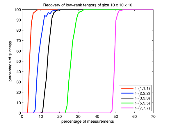
Figure 1: Numerical results for $10\times 10\times 10$ tensors with same $k$-ranks.

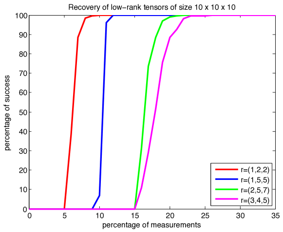
Figure 2: Numerical results for $10\times 10\times 10$ tensors with different $k$-ranks.

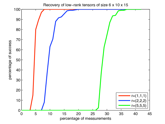
Figure 3: Numerical results for $6\times 10\times 15$ tensors with same $k$-ranks.

Figure 4: Numerical results for tensor IHT algorithm.

Table 1 complements Figure 4. With $\%_{\max}$ we denote the maximal percentage of measurements for which we did not manage to recover even one tensor out of $200$. The minimal percentage of measurements for full recovery is denoted by $\%_{\min}$. The last column represents the number of iterations needed for full recovery with $m=\lceil n_{1}n_{2}n_{3}\frac{\%_{\min}}{100}\rceil$ number of measurements.

Table 1: Numerical results for tensor IHT algorithm.

$\,n_{1}\times n_{2}\times n_{3}\,$	rank	$\%_{\max}$	$\%_{\min}$	# of iterations for $\%_{\min}$
$10\times 10\times 10\,$	$\,(1,1,1)\,$	$3$	$9$	$321$
$10\times 10\times 10$	$(2,2,2)$	$6$	$20$	$185$
$10\times 10\times 10$	$(3,3,3)$	$10$	$21$	$337$
$10\times 10\times 10$	$(5,5,5)$	$23$	$33$	$547$
$10\times 10\times 10$	$(7,7,7)$	$47$	$54$	$1107$
$10\times 10\times 10$	$(1,2,2)$	$5$	$10$	$588$
$10\times 10\times 10$	$(1,5,5)$	$9$	$12$	$1912$
$10\times 10\times 10$	$(2,5,7)$	$15$	$22$	$696$
$10\times 10\times 10$	$(3,4,5)$	$15$	$26$	$384$
$6\times 10\times 15$	$(1,1,1)$	$3$	$8$	$511$
$6\times 10\times 15$	$(2,2,2)$	$7$	$20$	$214$
$6\times 10\times 15$	$(5,5,5)$	$26$	$37$	$501$

5 Concluding remarks

In this chapter we considered low rank tensor recovery for hierarchical tensors extending the classical Tucker format to a multi-level framework. For low ranks, this model can break the curse of dimensionality. Its number of degrees of freedom scale like $\mathcal{O}(ndr+dr^{3})\ll\mathcal{O}(n^{d})$ and $\mathcal{O}(ndr^{2})$ for TT tensors instead of $\mathcal{O}(n^{d})$. Under the assumption of a tensor restricted isometry property, we have shown local convergence for Riemannian gradient iterations and global convergence under a certain condition on the iterates of the tensor iterative hard thresholding algorithm for hierarchical tensors, including the classical Tucker format as well as tensor trains. For instance for TT tensors, an estimate of the TRIP for Gaussian measurement maps was provided that requires the number of measurements to scale like $m\sim ndr^{2}\log(dr)$. However, it is still not clear whether the logarithmic factor is needed.

Let us finally mention some open problems. One important task is to establish global convergence to the original tensor of any of the discussed algorithms, without additional assumptions such as (21) on the iterates. In addition, robustness and stability for the Riemannian gradient method are still open. Further, also the TRIP related to general HT tensors for Gaussian measurement maps is not yet established. Since the TRIP does not hold for the completion problem, it is not clear yet whether a low rank tensor can be recovered from less than $\mathcal{O}(n^{d/2})$ entries.

References

- (1) Absil, P.-A., Mahony, R.E., Sepulchre, R.: Optimization algorithms on matrix manifolds. Foundations of Computational Mathematics 10, 241–244 (2010)
- (2) Arnold, A., Jahnke, T.: On the approximation of high-dimensional differential equations in the hierarchical Tucker format. BIT Numerical Mathematics 54, 305–341 (2014)
- (3) Beck, M.H., Jäckle, A., Worth, G.A., Meyer, H.-D.: The multi-configuration time-dependent Hartree (MCTDH) method: a highly efficient algorithm for propagating wavepackets. Phys. Reports 324, 1–105 (2000)
- (4) Beylkin, G., Garcke, J., Mohlenkamp, M.J.: Multivariate regression and machine learning with sums of separable functions. SIAM J. Sci. Comput. 31, 1840–1857 (2009)
- (5) Beylkin, G., Mohlenkamp, M.J.: Algorithms for numerical analysis in high dimensions. SIAM J. Sci. Comput. 26, 2133–2159 (2005)
- (6) Bhatia, R.: Matrix Analysis. Graduate Texts in Mathematics 169, Springer (1997)
- (7) Blumensath, T., Davies, M.: Iterative hard thresholding for compressed sensing. Applied and Computational Harmonic Analysis 27, 265–274 (2009)
- (8) Blumensath, T., Davies, M.: Iterative thresholding for sparse approximations. J. Fourier Anal. Appl. 14, 629–654 (2008)
- (9) Candès, E.J., Recht, B.: Exact matrix completion via convex optimization. Found. Comput. Math. 9, 717-772 (2009)
- (10) Candès, E.J., Tao, T.: The power of convex relaxation: near-optimal matrix completion. IEEE Trans. Inform. Theory 56, 2053–2080 (2010)
- (11) Candès, E.J., Plan, Y.: Tight oracle bounds for low-rank matrix recovery from a minimal number of random measurements. IEEE Trans. Inform. Theory 57, 2342-2359 (2011)
- (12) Carlini, E., Kleppe, J.: Ranks derived from multilinear maps. Journal of Pure and Applied Algebra 215, 1999–2004 (2011)
- (13) Da Silva, C., Herrmann, F.J.: Hierarchical Tucker tensor optimization - Applications to tensor completion. In Proc. 10th International Conference on Sampling Theory and Applications (2013)
- (14) De Lathauwer, L., De Moor, B., Vandewalle, J.: A multilinear singular value decomposition. SIAM J. Matrix Anal. Appl. 21: 1253–1278 (2000)
- (15) Eldar, Y.C., Kutyniok, K. (Eds.): Compressed Sensing : Theory and Applications. Cambridge Univ. Press (2012)
- (16) Falcó, A., Hackbusch, W.: On minimal subspaces in tensor representations. Found. Comput. Math. 12, 765–803 (2012)
- (17) Falcó, A., Hackbusch, W., Nouy, A.: Geometric structures in tensor representations. Tech. Rep. 9, MPI MIS Leipzig (2013)
- (18) Fazel, M.: Matrix rank minimization with applications. PhD thesis, Stanford University, CA (2002)
- (19) Foucart, S., Rauhut, H.: A Mathematical Introduction to Compressive Sensing. Applied and Numerical Harmonic Analysis, Birkhäuser (2013)
- (20) Friedland, S., Lim, L.-H.: Tensor nuclear norm and bipartite separability. In preparation
- (21) Friedland, S., Ottaviani, G.: The number of singular vector tuples and uniqueness of best rank-one approximation of tensors. To appear in Foundations of Computational Mathematics
- (22) Gandy, S., Recht, B., Yamada, I.: Tensor completion and low-n-rank tensor recovery via convex optimization. Inverse Problems 27, 025010 (2011)
- (23) Grasedyck, L.: Hierarchical singular value decomposition of tensors. SIAM. J. Matrix Anal. & Appl. 31, 2029–2054 (2010)
- (24) Grasedyck, L., Kressner, D., Tobler, C.: A literature survey of low-rank tensor approximation techniques. GAMM-Mitteilungen 36, 53–78 (2013)
- (25) Gross, D.: Recovering low-rank matrices from few coefficients in any basis. IEEE Trans. Inform. Theory 57, 1548-1566 (2011)
- (26) Hackbusch, W.: Numerical tensor calculus. Acta Numerica 23, 651–742 (2014)
- (27) Hackbusch, W.: Tensor spaces and numerical tensor calculus. Springer series in computational mathematics 42 (2012)
- (28) Hackbusch, W.: Tensorisation of vectors and their efficient convolution. Numer. Math. 119, 465–488 (2011)
- (29) Hackbusch, W., Kühn, S.: A new scheme for the tensor representation. J. Fourier Anal. Appl. 15, 706–722 (2009)
- (30) Hackbusch, W., Schneider, R.: Tensor spaces and hierarchical tensor representations. In preparation
- (31) Haegeman, J., Osborne, T., Verstraete, F.: Post-matrix product state methods: to tangent space and beyond. Physical Review B 88, 075133 (2013)
- (32) Hastad, J.: Tensor rank is NP-complete. J. of Algorithms 11, 644–654 (1990)
- (33) Hillar, C.J., Lim, L.-H.: Most tensor problems are NP hard. J. ACM 60, 45:1–45:39 (2013)
- (34) Holtz, S., Rohwedder, T., Schneider, R.: On manifolds of tensors of fixed TT rank. Numer. Math. 120, 701–731 (2012)
- (35) Holtz, S., Rohwedder, T., Schneider, R.: The alternating linear scheme for tensor optimisation in the tensor train format. SIAM J. Sci. Comput. 34, A683 – A713 (2012)
- (36) Huang, B., Mu, C., Goldfarb, D., Wright, J.: Provable low-rank tensor recovery. http://www.optimization-online.org/DB_FILE/2014/02/4252.pdf (2014)
- (37) Lim, L.-H., De Silva, V.: Tensor rank and the ill-posedness of the best low-rank approximation problem. SIAM J. Matrix Anal. & Appl. 30, 1084–1127 (2008)
- (38) Kolda, T.G., Bader, B.W.: Tensor decompositions and applications. SIAM Review 51, 455–500 (2009)
- (39) Kreimer N., Sacchi, M.D.: A tensor higher-order singular value decomposition for prestack seismic data noise reduction and interpolation. Geophysics 77, V113-V122 (2012)
- (40) Kressner, D., Steinlechner, M., Vandereycken, B.: Low-rank tensor completion by Riemannian optimization. BIT Numerical Mathematics 54, 447–468 (2014)
- (41) Landsberg, J.M.: Tensors: geometry and applications. Graduate Studies in Mathematics 128, AMS, Providence, RI (2012)
- (42) Legeza, Ö., Rohwedder, T., Schneider, R., Szalay, S.: Tensor product approximation (DMRG) and coupled cluster method in quantum chemistry. Many-Electron Approaches in Physics, Chemistry and Mathematics, 53–76, Springer (2014)
- (43) Levin, J.: Three-Mode Factor Analysis. Ph.D. thesis, University of Illinois, Urbana (1963)
- (44) Liu, J., Musialski, P., Wonka, P., Ye, J.: Tensor completion for estimating missing values in visual data. Transactions of Pattern Analysis & Machine Inteligence (PAMI) 35, 208–220 (2012)
- (45) Liu, Y., Shang, F.: An efficient matrix factorization method for tensor completion. IEEE Signal Processing Letters 20, 307–310 (2013)
- (46) Lubich, C.: From quantum to classical molecular dynamics: Reduced methods and numerical analysis. Zürich Lectures in advanced mathematics 12, EMS (2008)
- (47) Lubich, C., Rohwedder, T., Schneider, R., Vandereycken, B.: Dynamical approximation by hierarchical Tucker and Tensor-Train tensors. SIAM J. Matrix Anal. Appl. 34, 470–494 (2013)
- (48) Mu, C., Huang, B., Wright, J., Goldfarb, D.: Square deal: Lower bounds and improved relaxations for tensor recovery. arxiv.org/abs/1307.5870v2 (2013)
- (49) Oseledets, I.V.: A new tensor decomposition. Doklady Math. 80, 495–496 (2009)
- (50) Oseledets, I.V.: Tensor-train decomposition. SIAM J. Sci. Comput. 33, 2295–2317 (2011)
- (51) Oseledets, I.V., Tyrtyshnikov, E.E.: Algebraic wavelet transform via quantics tensor train decomposition. SIAM J. Sci. Comput. 33, 1315–1328 (2011)
- (52) Oseledets, I.V., Tyrtyshnikov, E.E.: Breaking the curse of dimensionality, or how to use SVD in many dimensions. SIAM J. Sci. Comput. 31, 3744–3759 (2009)
- (53) Rauhut, H., Schneider, R., Stojanac, Ž.: Tensor recovery via iterative hard thresholding. In Proc. 10th International Conference of Sampling Theory and Appl. (2013)
- (54) Rauhut, H., Schneider, R., Stojanac, Ž.: Low rank tensor recovery via iterative hard thresholding. In preparation
- (55) Recht, B., Fazel, M., Parrilo, P.A.: Guaranteed minimum-rank solution of linear matrix equations via nuclear norm minimization. SIAM Rev. 52, 471–501 (2010)
- (56) Recht, B.: A simpler approach to matrix completion. J. Mach. Learn. Res. 12, 3413-3430 (2011)
- (57) Rohwedder, T., Uschmajew, A.: On local convergence of alternating schemes for optimization of convex problems in the tensor train format. SIAM J. Numer. Anal. 51, 1134–1162 (2013)
- (58) Romera-Paredes, B., Pontil, M.: A new convex relaxation for tensor completion. NIPS 26, 2967–2975 (2013)
- (59) Schneider, R., Uschmajew, A.: Approximation rates for the hierarchical tensor format in periodic Sobolev spaces. Journal of Complexity 30, 56–71 (2014)
- (60) Schneider, R., Uschmajew, A.: Convergence results for projected line-search methods on varieties of low-rank matrices via Łojasiewicz inequality. arxiv.org/abs/1402.5284v1
- (61) Schollwöck, U.: The density-matrix renormalization group in the age of matrix product states, Annals of Physics (NY) 326, 96-192 (2011)
- (62) Signoretto, M., De Lathauwer, L., Suykens, J.A.K.: Nuclear norms for tensors and their use for convex multilinear estimation. Int. Rep. 10–186, ESAT-SISTA, K. U. Leuven (2010)
- (63) Signoretto, M., Tran Dinh, Q. , De Lathauwer, L., Suykens, J.A.K.: Learning with tensors: a framework based on convex optimization and spectral regularization. Machine Learning 94, 303–351 (2014)
- (64) Tanner, J., Wei, K.: Normalized iterative hard thresholding for matrix completion. SIAM J. Scientific Computing 35, S104–S125 (2013)
- (65) Tucker, L.R.: Some mathematical notes on three-mode factor analysis. Psychometrika 31, 279–311 (1966)
- (66) Tucker, L.R.: Implications of factor analysis of three-way matrices for measurement of change. Problems in Measuring Change. Harris, C.W. (Eds.), University of Wisconsin Press, 122–137 (1963)
- (67) Tucker, L.R.: The extension of factor analysis to three-dimensional matrices. Contributions to Mathematical Psychology. Gulliksen, H., Frederiksen N. (Eds.), Holt, Rinehart & Winston, New York, 110–127 (1964)
- (68) Uschmajew, A.: Well-posedness of convex maximization problems on Stiefel manifolds and orthogonal tensor product approximations. Numer. Math. 115, 309–331 (2010)
- (69) Uschmajew, A. and Vandereycken, B.: The geometry of algorithms using hierarchical tensors. Linear Algebra and its Appl. 439, 133–166 (2013)
- (70) Vandereycken, B.: Low-rank matrix completion by Riemannian optimization. SIAM J. Optim. 23, 1214–1236 (2013)
- (71) Vershynin, R.: Introduction to the non-asymptotic analysis of random matrices. Compressed sensing: Theory and Applications. Eldar, C.Y., Kutyniok, G. (Eds.), Cambridge Univ. Press, Cambridge, 210–268 (2012)
- (72) Vidal, G.: Efficient classical simulation of slightly entangled quantum computations. Phys. Rev. Lett. 91, 147902 (2003)
- (73) Wang, H., Thoss, M.: Multilayer formulation of the multi-configuration time-dependent Hartree theory. J. Chem. Phys. 119, 1289–1299 (2003)
- (74) Wen, Z., Yin, W., Zhang, Y.: Solving a low-rank factorization model for matrix completion by a nonlinear successive over-relaxation algorithm. Math. Prog. Comp. 4, 333–361 (2012)
- (75) White, S.: Density matrix formulation for quantum renormalization groups. Phys. Rev. Lett. 69, 2863–2866 (1992)
- (76) Xu, Y., Hao, R., Yin, W., Su, Z.: Parallel matrix factorisation for low-rank tensor completion. UCLA CAM, 13-77 (2013)
- (77) Xu, Y., Yin, W.: A block coordinate descent method for regularized multiconvex optimization with applications to nonnegative tensor factorization and completion. SIAM Journal on Imaging Sciences 6, 1758–1789 (2013)