Optimizing Passive Quantum Clocks

Abstract

We describe protocols for passive atomic clocks based on quantum interrogation of the atoms. Unlike previous techniques, our protocols are adaptive and take advantage of prior information about the clock’s state. To reduce deviations from an ideal clock, each interrogation is optimized by means of a semidefinite program for atomic state preparation and measurement whose objective function depends on the prior information. Our knowledge of the clock’s state is maintained according to a Bayesian model that accounts for noise and measurement results. We implement a full simulation of a running clock with power-law noise models and find significant improvements by applying our techniques.

I Introduction

Atomic clocks continue to make great strides in accuracy and stability. Passive atomic clocks compare the frequency of an external, “flywheel” oscillator to that of a reference transition in an atom, the atomic standard. In view of the increasing impact of quantum information science and the associated rapid growth of quantum control capabilities, there has been substantial interest in the possibility of exploiting quantum effects and quantum algorithms for further improvements in clock precision. Whereas measurements with $N$ atoms in independent states yield errors that scale as $1/\sqrt{N}$ (the so called “standard quantum limit”, SQL), protocols using entangled quantum states can yield errors that scale as $1/N$, the fundamental “Heisenberg limit”. Here, we are interested in optimizing such quantum protocols and evaluating their performance in clocks subject to realistic noise.

The first proposals to beat the SQL used spin squeezed states Wineland et al. (1992); Kitagawa and Ueda (1993); Wineland et al. (1994). Not long afterward, Bollinger et. al. Bollinger et al. (1996) demonstrated that the Heisenberg bound could be achieved by using maximally entangled states. Even though such states achieve optimal scaling in the noiseless regime, it was shown Huelga et al. (1997) that such states cannot beat the SQL in the presence of atomic decoherence. This spurred research into protocols that perform well even in noisy systems; for example, see Refs. Berry et al. (2009); Higgins et al. (2007); Huver et al. (2008); Luis (2002); Dorner (2012); Dorner et al. (2009). However, in most modern clocks, the dominant sources of noise are random fluctuations of the external oscillator (see below) and not atomic decoherence. Refs. Wineland et al. (1998); André et al. (2004) were among the first to study clock optimization in the presence of this type of noise. In Ref. André et al. (2004), an error scaling of $1/N^{2/3}$ is obtained by optimizing over a family of spin squeezed states.

The standard approach to the clock optimization problem involves optimizing individual measurements of the atomic standard with respect to fixed objective functions. In this spirit, Refs. Bužek et al. (1999); Demkowicz-Dobrzański (2011); van Dam et al. (2007); Macieszczak et al. (2013) derive states and measurements that are optimal under certain sets of assumptions by optimizing a cost function that approximates a clock’s performance. In Ref. Rosenband (2012), various such measurement protocols are compared in a Monte Carlo simulation of a clock subject to $1/\omega$ noise. For a two qubit clock, it was estimated that the best protocol would result in a $15$-$20\,\%$ improvement in Allan variance, a standard measure of long-term clock performance. However, none of the simulated protocols were optimal, so despite this work and other work in quantum metrology (for a review, see Giovannetti et al. (2011)), it is yet to be seen how much can be gained by fully utilizing quantum resources.

Clocks are used to construct a time scale by marking, or timestamping, a set of events labeled $\{1,2,\ldots n\}$ with time values $\{t_{1},t_{2}\ldots t_{n}\}$. Time is defined in terms of a transition frequency $\Omega$ of a chosen atomic frequency standard; if the standard could be measured directly, these assignments could be made trivially by counting cycles of the selected transition. However, in practice, such a measurement is often difficult, and therefore, an external oscillator or “flywheel” at frequency $\omega$ near $\Omega$ is measured rather than the standard. Clocks that use such an oscillator are referred to as “passive” atomic clocks. A measurement of the phase deviation of the external oscillator is then required to assign timestamps accurately. Such a measurement involves interactions between the external oscillator and the standard. The part of the protocol involving one state preparation followed by evolution and a measurement is called an interrogation. Our goal here, and the goal of the work discussed above, is to optimize passive clocks by deriving protocols that maximize the information gained during each interrogation.

Here we consider interrogations involving a state preparation, a free evolution and a measurement, where the state preparation and measurement take negligible time. We gain information about the time-averaged frequencies during interrogations. Because the interrogations necessarily yield incomplete information and the external oscillator is subject to noise, the frequencies are described by probability distributions. Given a model of the noise affecting our systems, our knowledge of the state of the system after $n$ interrogations is described by the probability distribution $p(\langle\omega\rangle_{1},\langle\omega\rangle_{2},\ldots\langle\omega\rangle_{n}|a_{1},a_{2},\ldots a_{n})$, where $\langle\omega\rangle_{k}$ is the time-averaged frequency of the external oscillator during interrogation $k$ and $a_{k}$ is the measurement outcome obtained at the end of the $k$’th interrogation. To avoid confusion between time-averaging for a particular instance of the noise model and computing expected values based on the noise model’s probability distribution, we drop the averaging brackets and identify $\omega_{k}$ with the time-averaged frequency during the $k$’th interrogation. Note that the $\omega_{k}$ are random variables that can be expressed as integrals over the instantaneous frequencies. We abbreviate their distributions as $p(\omega_{1},\omega_{2},\ldots\omega_{n}|a_{1},a_{2},\ldots a_{n})=p(\bm{\omega_{n}}|\bm{a_{n}})$, where $\bm{\omega_{n}}$ and $\bm{a_{n}}$ refer to the sequence of time-averaged frequencies and the sequence of measurement outcomes obtained during interrogations $1$ through $n$. Unless required for clarity, we drop the adjective “time-averaged” when referring to the $\omega_{k}$.

Our approach improves on prior work in several ways. First, observe that the optimal choice for the $n+1$’th interrogation depends on $p(\bm{\omega_{n}}|\bm{a_{n}})$. Given a good model of the noise, it is possible to keep track of these conditional probability distributions. Traditional interrogations do not take advantage of this information; many use the same, fixed strategy for each interrogation. Furthermore, most analyses related to the Heisenberg limit apply only in the absence of preexisting information. In contrast, our interrogations are dynamic. They are tailored to our knowledge of the clock’s state by making use of available prior information. Second, we jointly derive quantum state preparations and measurements with a semidefinite program. We refer to the quantum state preparation and measurement as the quantum algorithm used by the interrogation. The semidefinite program gives us freedom in choosing our optimization criteria, which are expressed in the form of state-dependent cost functions. Given such a function, the semidefinite program determines the optimal quantum algorithm without being limited to specific cost functions or a restrictive class of states and measurements. Third, we prove that this flexibility in choosing cost functions is required in order to minimize the error in the total elapsed-time estimates. For most noise models, memory effects imply that a simple criterion based on the difference between the current frequency of the oscillator and the estimated one does not suffice.

The remainder of this paper is structured as follows: We discuss atomic interrogation and detail the properties of the types of noise assumed to affect the external oscillator. We then describe our optimization criteria and explain how we dynamically derive the quantum algorithm for the next interrogation. Finally, we implement our protocol on full simulations of clocks subject to various power-law noise models and demonstrate improvements over prior, fixed protocols. Throughout, we assume full quantum control over the atomic system and that the only source of noise is statistical fluctuations of the external oscillator. While this latter assumption is sensible for many modern clocks, if necessary, our scheme can be adapted to account for decoherence Mullan and Knill (2012). We conclude with a discussion of further work needed to apply our theoretical methods to experimental passive clocks.

II Interrogations

Here, we consider the atoms as idealized two-level systems with standard basis ${|}{0}{\rangle}$ and ${|}{1}{\rangle}$ and use the usual conventions for operators acting on these systems. Once a quantum algorithm has been decided on, an interrogation prepares the atoms in an initial state ${|}{\psi}{\rangle}$ via the application of a chosen unitary, ${|}{\psi}{\rangle}=U{|}{\mathbf{0}}{\rangle}$ to the standard starting state ${|}{\mathbf{0}}{\rangle}$. The inital state preparation is followed by a period of free evolution of duration $T$, which effects a $z$ rotation $R_{z}((\omega-\Omega)T)$ by an angle of $(\omega-\Omega)T$. Thus we transform ${|}{\psi}{\rangle}$ to ${|}{\psi^{\prime}}{\rangle}=R_{z}((\omega-\Omega)T)U{|}{\textbf{0}}{\rangle}$. The angle of the rotation relates the external oscillator’s frequency to that of the atomic standard. We assume that the time needed to apply unitaries is negligible compared to the period of free evolution. Afterward, the atomic state ${|}{\psi^{\prime}}{\rangle}$ is measured with a complete positive operator-valued measure (POVM) $\{P_{a}\}_{a}$. Traditional interrogations choose the same initial state and, except for a phase, the same POVM every time. For example, the widely used Ramsey method prepares $N$ atoms in the state $\left(\begin{smallmatrix}1/\sqrt{2}\\ -i/\sqrt{2}\end{smallmatrix}\right)^{\otimes N}$ and, after a period of free evolution, measures each atom independently in the ${|}{+}{\rangle}$, ${|}{-}{\rangle}$ basis. Here we allow $U$ and the POVM to be chosen differently in each interrogation. Note that the quantum algorithm of an interrogation can be generalized to ${|}{\psi^{\prime}}{\rangle}=R_{z}((\omega-\Omega)T)U(t_{f})\ldots U(1)R_{z}((\omega-\Omega)T)U(0){|}{\mathbf{0}}{\rangle}$, followed by a measurement of ${|}{\psi^{\prime}}{\rangle}$ with a POVM. These multi-round algorithms can outperform single-round ones. However, they are more difficult to implement in practice. Although our optimization procedures can derive such algorithms, we do not consider them here.

Since all measurements will be referenced to $\Omega$, from now on we take $\omega$ to be the frequency deviation from $\Omega$ rather than the absolute frequency. We normally omit the modifier “deviation”.

III Noise Models

Noise affects the external oscillator at all times, competing with the knowledge gained from measurements. The noise model determines the prior distributions to be used for the frequencies. Here, we assume that it can be approximated by a continuous, multivariate Gaussian random process characterized by a spectral density, $S(\omega)$. It has been determined that power law noise is a good approximation on relevant frequency ranges, in which case $S(\omega)\propto\omega^{\alpha}$. Relevant exponents are $\alpha\in[-4,2]$ Allan (1966); Riley (2008). For example, $1/\omega$ noise is common for cavity-locked optical oscillators Numata et al. (2004). Gaussian noise processes are characterized by their means and covariances. For our applications, the unconditional means are assumed to be zero. The $\omega_{k}$ can then be characterized as joint Gaussian random variables characterized by their covariances. We denote the covariance between the external oscillator’s frequencies at times $s$ and $s^{\prime}$ as $\mathbf{Cov}(\omega(s),\omega(s^{\prime}))$. Strictly speaking, $\omega$ and the covariances need to be interpreted as generalized functions of time. As we define them below, their domain is restricted to test functions with zero mean. In particular, we compute covariances only for differences between interval averages. For point values or for other averages, the expressions given may be undefined or fail to give non-negative variances. We focus on frequency changes relative to an initial frequency, where for the purpose of defining our priors, the initial frequency is taken to be zero. With respect to the experimentally relevant frequencies, we define the covariance matrix $C$ according to

$$\begin{array}[b]{rl@{}l}\displaystyle C_{i,j}&=\mathbf{Cov}(&\omega_{i}-\omega_{0},\omega_{j}-\omega_{0})\\ &=\mathbf{Cov}(&\langle\omega(s)\rangle_{s\in I_{i}}-\langle\omega(s)\rangle_{s\in I_{0}},\\ &&\langle\omega(s)\rangle_{s\in I_{j}}-\langle\omega(s)\rangle_{s\in I_{0}}),\end{array}$$ (1)

where $I_{i}$ is the $i$’th interrogation interval $I_{i}=[t_{i},t_{i+1}]$, and $I_{0}=[t_{0},t_{1}]$ is an interval before the first interrogation. The length of the $i$’th interval is defined as $T_{i}$.

To compute $C_{i,j}$ for $-3<\alpha<-1$ we can formally express $\mathbf{Cov}(\omega(s),\omega(s^{\prime}))=-\frac{h_{\alpha}}{2}|s-s^{\prime}|^{-\alpha-1}$ where $h_{\alpha}$ is an $\alpha$ dependent scale factor. For $\alpha=-1$, $\mathbf{Cov}(\omega(s),\omega(s^{\prime}))=-2h_{-1}\ln|s-s^{\prime}|$ Fyodorov et al. (2009). The $C_{i,j}$ can then be computed by expanding to a sum of terms of the form

$$\mathbf{Cov}(\langle\omega(s)\rangle_{s\in I_{k}},\langle\omega(s)\rangle_{s\in I_{l}})$$ (2)

$$= \frac{1}{T_{k}}\frac{1}{T_{l}}\int_{t_{k}}^{t_{k+1}}ds\int_{t_{l}}^{t_{l+1}}ds^{\prime}\mathbf{Cov}(\omega(s),\omega(s^{\prime})).$$

For $\alpha\leq-3$, one can view the power spectrum as a $2r$’th distributional derivative of a power spectrum with $\alpha\in(-3,-1]$ and multiply the formal expression for $\mathbf{Cov}(\omega(s),\omega(s^{\prime}))$ by $(-1)^{r}(s-s^{\prime})^{2r}$ to apply similar techniques. For $\alpha>-1$, the distributional derivatives are applied to $\mathbf{Cov}(\omega(s),\omega(s^{\prime}))$. In both cases, care must be taken to ensure that covariances are computed only for quantities in the appropriate domain where they are well-defined and positive-definite.

IV Optimizing Interrogations

The quality of our true-time estimates depends on how well we estimate the phase difference between the external oscillator and an ideal oscillator with frequency that of the atomic standard. We therefore wish to choose phase estimates, $\theta^{*}_{n}$, that minimize the expectation

$$\mathbf{E}\left(\left(\theta_{n}-\theta^{*}_{n}\right)^{2}\right),$$ (3)

where $\theta_{n}$ is the cumulative phase difference of the external oscillator after interrogation $n$, $\theta_{n}=\omega_{1}T_{1}+\omega_{2}T_{2}\ldots+\omega_{n}T_{n}$, and $\theta^{*}_{n}$ is our estimate of this phase. The expectation is taken over the noise model and we use the symbol $\mathbf{E}$ to denote the expectation. The expression in (3) is evaluated according to

$$\mathbf{E}\left(\left(\theta_{n}-\theta^{*}_{n}\right)^{2}\right)=\int(\theta_{n}-\theta_{n}^{*})^{2}p(\theta_{n}|\bm{a_{n}})d\theta_{n},$$ (4)

where $p(\theta_{n}|\bm{a_{n}})$ can be obtained from $p(\bm{\omega_{n}}|\bm{a_{n}})$. The choice $\theta^{*}_{n}=\mathbf{E}(\theta_{n}|\bm{a_{n}})$ minimizes Eq. (4), giving a value equal to the posterior variance, $V_{n}=\mathbf{V}(\theta_{n}|\bm{a_{n}})$. Here, we use the symbol $\mathbf{V}$ to denote the variance. Our goal is therefore to construct quantum algorithms that minimize the expected posterior variance increase $\Delta V_{n}$ given by

$$\Delta V_{n} =\sum_{a_{n}}(V_{n}-V_{n-1})p(a_{n}|a_{1}\ldots a_{n-1})$$

$$=\sum_{a_{n}}\mathbf{V}(\theta_{n-1}+\omega_{n}T_{n}|a_{1}\ldots a_{n})p(a_{n}|a_{1}\ldots a_{n-1})-\mathbf{V}(\theta_{n-1}|a_{1}\ldots a_{n-1})$$ (5)

after the $n$’th interrogation.

For each interrogation, we obtain the optimal quantum algorithm by extending the procedure described in Ref. Mullan and Knill (2012). There, we relate the operation of an atomic clock to quantum complexity theory, specifically a generalization of the adversary method, and use this relationship to calculate quantum algorithms that optimize the expected posterior cost of an interrogation,

$$\mathbf{E}(C)=\sum_{a}\int C(\omega,a)p(\omega,a)d\omega.$$ (6)

Here, $\omega$ is the frequency deviation of the external oscillator during the interrogation of interest. While we can optimize the cost for any reasonable cost function, the choice is determined by how we quantify clock performance. A traditional choice and the one emphasized in Ref. Mullan and Knill (2012) is $C(\omega,a)=(\omega-g(a))^{2}$, where the $g(a)$ are frequency estimates depending on the (arbitrarily labeled) measurement outcomes $a$. The estimates can be chosen so that minimization of $\mathbf{E}(C)$ for the $n$’th interrogation minimizes the expected posterior variance of $\omega_{n}T_{n}$. However, for noise models with memory, this does not minimize the expected posterior total variance increase $\Delta V_{n}$. This is because in general, $\mathbf{V}(\theta_{n}|\bm{a_{n}})$ is not the same as $\mathbf{V}(\omega_{1}T_{1}|a_{1})+\mathbf{V}(\omega_{2}T_{2}|a_{2})+\ldots\mathbf{V}(\omega_{n}T_{n}|a_{n})$, due to correlations between the $\omega_{i}$’s. In App. A, we prove that the following adaptively chosen cost function has the desired effect of minimizing $\Delta V_{n}$:

$$C(\omega,a)=(\omega T-g(a))^{2}+2(\omega T-g(a))\mathbf{E}(\theta-\mathbf{E}(\theta)|\omega),$$ (7)

where $\theta$ is the phase deviation just before the interrogation of interest and $\omega$ is the frequency of the oscillator during this interrogation. The expectations in the cost function are implicitly conditioned on every earlier measurement outcome. The minimum $\Delta V_{n}$ is achieved in the continuum limit of the SDP, where the measurement outcome labels are possible average frequencies $\omega_{n}$ and $g$ is the identity function. The implemented SDPs involve discretization. Ref. Mullan and Knill (2012) shows that the discretization error can be made arbitrarily small and how to bound it.

In order to derive algorithms that minimize $\Delta V_{n}$, we need access to $p(\bm{\omega_{n}}|\bm{a_{n-1}})$ before the $n$’th interrogation. This requires that we correctly maintain and update such a distribution as a clock runs. For the moment, we assume that it is possible to keep track of these continous and high-dimensional distributions exactly. Later, we discuss how to discretize and truncate them in practice. Fig. 1 depicts the evolution of this probability distribution associated with the first interrogation. In general, before the $n$’th interrogation, we have access to $p(\bm{\omega_{n-1}}|\bm{a_{n-1}})$ as computed from the previous interrogation or, for $n=1$, from the initial conditions. The $n$’th interrogation requires that we (1) compute the prior $p(\bm{\omega_{n}}|\bm{a_{n-1}})$ according to the noise model and previously determined priors and measurement outcomes, (2) derive and apply a quantum algorithm based on this distribution, and (3) compute the posterior distribution $p(\bm{\omega_{n}}|\bm{a_{n}})$ from the prior and measurement outcome $a_{n}$. In more detail, the procedure is:

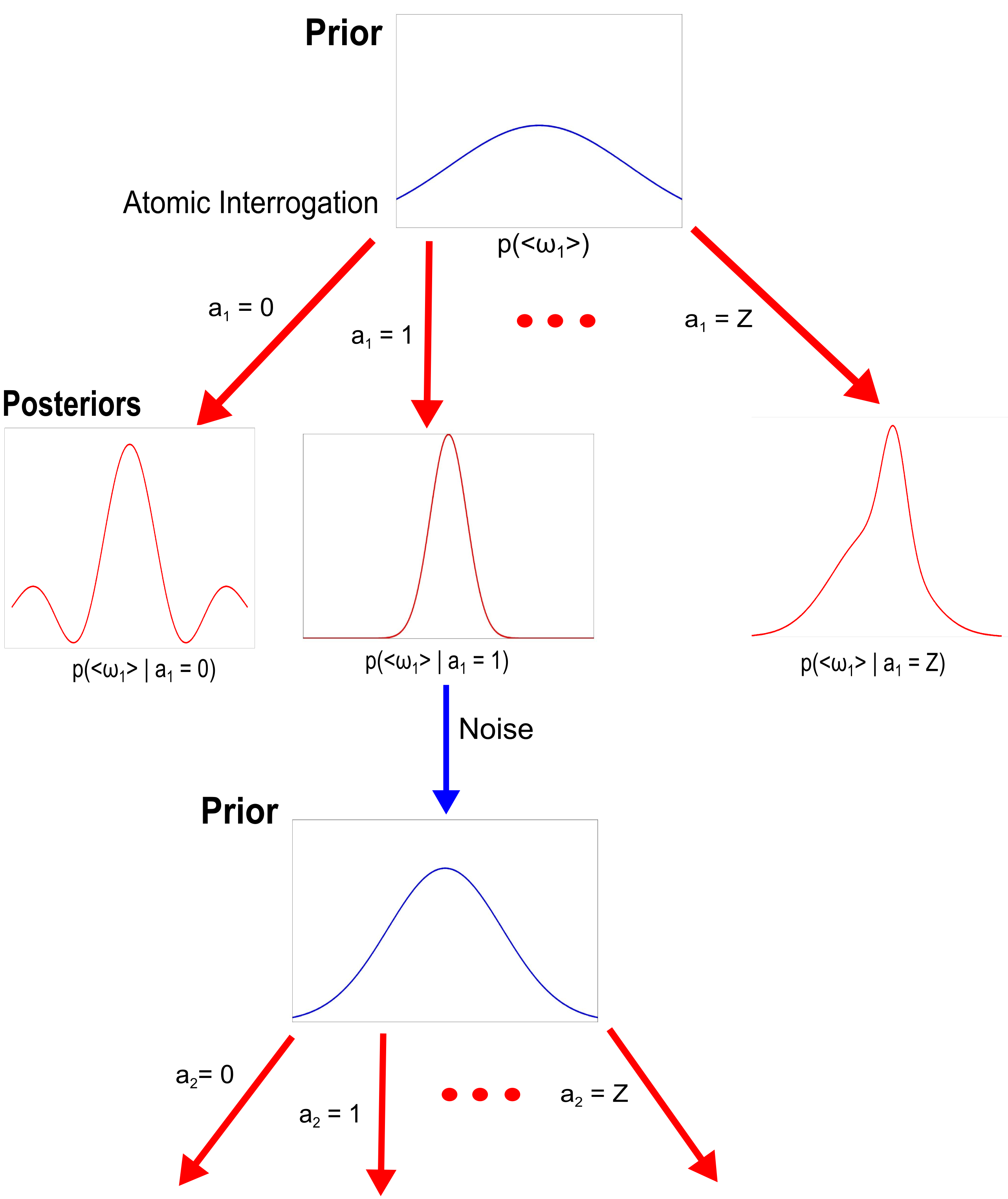
Figure 1: Evolution of the external oscillator’s posterior probability distribution in a clock protocol. The probability distribution at the top characterizes the frequency of the clock during interrogation $1$. A measurement of the atomic standard at time $t_{1}$, with $Z$ element POVM $\{P_{a}\}_{a}$ then yields measurement outcome $a_{1}$ with probability $p(a_{1})$. This can be used to compute the posterior distribution $p(\omega_{1}|a_{1})$. (In the figure, we imagine that we obtain measurement outcome $a_{1}=1$.) Noise then affects the clock for duration $T_{2}$; this decreases our knowledge of the external oscillator’s frequency, widening the probability distribution. The resulting prior probability distribution corresponds to the frequency of the classical oscillator during interrogation $2$. This procedure is repeated indefinitely.

1. Compute the prior probability distribution $p(\bm{\omega_{n}}|\bm{a_{n-1}})$ according to

   $$p(\bm{\omega_{n}}|\bm{a_{n-1}})=p(\omega_{n}|\bm{\omega_{n-1}},\bm{a_{n-1}})p(\bm{\omega_{n-1}}|\bm{a_{n-1}}).$$ (8)

   For this purpose, note that $p(\omega_{n}|\bm{\omega_{n-1}},\bm{a_{n-1}})=p(\omega_{n}|\bm{\omega_{n-1}})$, so that it can be computed directly from the noise model’s covariance matrix.

2. From $p(\bm{\omega_{n}}|\bm{a_{n-1}})$, determine the cost function of Eq. (7) and apply the SDP of Ref. Mullan and Knill (2012) to compute an optimal algorithm consisting of a unitary matrix $U$ and a POVM $\{P_{a}\}_{a}$.

3. Given this algorithm, fill in the collection of distributions $p(a_{n}|\omega_{n})$ for each $\omega_{n}$.

4. Use the algorithm to interrogate the frequency standard for a time $T_{n}$. Obtain the actual measurement outcome $a^{*}_{n}$.

5. Assign $a_{n}=a^{*}_{n}$ and compute the posterior distribution needed for the next timestep according to

   $$p(\bm{\omega_{n}}|\bm{a_{n}}) =p(\omega_{n},\bm{\omega_{n-1}}|a_{n},\bm{a_{n-1}})$$

   $$=p(\omega_{n},\bm{\omega_{n-1}},a_{n}|\bm{a_{n-1}})/p(a_{n}|\bm{a_{n-1}})$$

   $$=p(\omega_{n},\bm{\omega_{n-1}}|\bm{a_{n-1}})p(a_{n}|\omega_{n},\bm{\omega_{n-1}},\bm{a_{n-1}})/p(a_{n}|\bm{a_{n-1}})$$

   $$=p(\bm{\omega_{n}}|\bm{a_{n-1}})p(a_{n}|\omega_{n})/p(a_{n}|\bm{a_{n-1}}).$$ (9)

   Here, we used the fact that $a_{n}$ is independent of $\bm{\omega_{n-1}}$ and $\bm{a_{n-1}}$ given $\omega_{n}$. The term $p(a_{n}|\bm{a_{n-1}})$ can be computed as

   $$p(a_{n}|\bm{a_{n-1}}) =\int d{\bm{\omega^{\prime}_{n}}}p(a_{n}|\bm{\omega^{\prime}_{n}},\bm{a_{n-1}})p(\bm{\omega^{\prime}_{n}}|\bm{a_{n-1}})$$

   $$=\int d{\bm{\omega^{\prime}_{n}}}p(a_{n}|\omega^{\prime}_{n})p(\bm{\omega^{\prime}_{n}}|\bm{a_{n-1}}).$$ (10)

6. Compute the posterior expectation $\mathbf{E}(\theta_{n}|\bm{a_{n}})$ of the phase $\theta_{n}=\theta_{n-1}+\omega_{n}T_{n}$. This is our estimate of the external oscillator’s phase after interrogation $n$ and may be used to assign timestamps.

Note that this procedure can be readily generalized if other information becomes available during an interrogation. Here, the part of the clock’s state relevant to timekeeping given the interrogation history is determined by the (true) frequencies $\omega_{n}$. In general, there may be other state variables we can exploit, in which case the relevant part of the state is given by more fundamental variables $s_{n}$ describing the state during the $n$’th interrogation. Also, after each interrogation, the best estimates of the phases $\theta_{k}$ for $k<n$ based on current information can change. Thus, it is beneficial to retroactively update these estimates also.

V Systematic Errors

There are three sources of error that arise in the above interrogation procedure: (1) Discretization error in the SDP used to construct each unitary and POVM, (2) discretization and truncation of $p(\bm{\omega_{n}}|\bm{a_{n}})$, and (3) incomplete knowledge of the true duration of each interrogation. The first issue was discussed in Ref. Mullan and Knill (2012); here, we discuss the other two.

To address the second source of error, note that the distributions of the $\omega_{n}$ are inherently continuous and must be discretized sufficiently finely. However, if we discretize the domain of $\omega_{n}$ with $P$ points, then the representation of the joint probability distribution grows by a factor of $P$ at every step; if $P$ is large, the strategy described above quickly becomes computationally infeasible. We therefore truncate the clock history by storing only a limited number of $\omega_{n}$, and marginalizing out old distributions as the clock progresses. Since most of the noise models discussed above contain long-term correlations, this procedure no longer represents these models faithfully. But the correlations typically fall off as a power law, so we may be justified in concluding that the impact on the performance of our protocol is limited, provided enough memory is maintained. The truncation indirectly affects the SDP. While the SDP does not explicitly require the full joint distribution, the cost function of Eq. (7) involves expectations of the cumulative phase $\theta_{n-1}$ and depends on the $\omega_{k}$ lost in truncation. In App. C we show how this expectation, and more generally, $\mathbf{E}(\theta_{n}^{k}|\omega_{n+1},\bm{a_{n}})$ for arbitrary $k$ can be updated without keeping full track of all $\omega_{k}$.

With regard to the third issue, so far we have fixed the duration of interrogation $n$ at $T_{n}$ and assumed that $T_{n}$ is the “real” duration. However, the end points of the interrogation are chosen by the experimenter based on the external oscillator or an auxiliary clock locked to the oscillator. In addition, the implementations of state preparation and measurement take finite time, adding additional uncertainty concerning the true duration of the implemented interrogation. The standard interrogation methods are normally insensitive to variations in $T_{n}$ and non-zero preparation and measurement intervals because the external oscillator’s frequency is constantly controlled to match the frequency standard. For our protocols, explicitly changing the external oscillator’s frequency within the memory time of the noise model would complicate the algorithm for keeping track of the relevant posterior probability distributions. With a free-running external oscillator, it is necessary to adapt the interrogation algorithms to minimize the effect of timing deviations. One adaptation involves simulating the effect of a locked oscillator. We also suggest that it is beneficial to adapt the SDP used to optimize the interrogations. How to implement both adaptations and the size of residual errors is discussed in the App. D.

VI Simulations

To test our protocol, we implemented a general-purpose Monte Carlo simulation of the external oscillator and used it in a simulated clock with the above protocol and update strategy. In these simulations, we used a constant interrogation duration $T$ throughout. To evaluate the simulated clocks, we compute the average square difference between the estimated average frequency and the true average frequency of the simulated external oscillator (the “square frequency error”), where both are cumulative time-averages from the start of the clock. We also compute the overlapping Allan variances given by

$$\sigma^{2}(mT)= \frac{1}{2(M-2m+1)}\times$$

$$\sum_{j=1}^{M-2m+1}(\langle\omega^{*}\rangle_{(j+m,m)}-\langle\omega^{*}\rangle_{(j,m)})^{2},$$ (11)

where $M$ is the total number of interrogations, each of equal duration $T$, $\langle\omega^{*}\rangle_{k,m}=\sum_{l=k}^{k+m-1}\omega^{*}_{l}/m$ and $\omega^{*}_{j}$ is the best estimate of $\omega_{j}$ given by the computed mean of the relevant posterior probability distributions. The Allan variance is what would actually be reported in an experimental realization of these clocks and does not depend on knowing the true frequencies.

Below (see Fig. 2), we compare our protocol to the Ramsey protocol, which is utilized by most atomic clocks today, and to that of Buzek et. al. Bužek et al. (1999). The latter is a fully quantum technique optimized for a uniform prior probability distribution of external oscillator frequencies. We limit our comparisons to clocks with low noise in order to reduce phase-slip errors that result in random frequency hops of size $2\pi/T$.

The traditional Ramsey protocol is used with an external oscillator that is controlled to have a frequency matching the atomic standard as closely as possible. To simplify noise model calculations, we do not adjust the external oscillator. Instead we compute the measurement phase directly, according to the computed means of the prior probability distribution for the frequencies. See the discussion of timing errors in App. D. Provided the noise model is a good representation of the external oscillator’s behavior, this is expected to perform better than the standard control strategies, so that our comparison is fair.

Fig. 2 compares our protocol to that of Ramsey and that of Buzek for a two-atom clock subject to Brownian motion ($\alpha=-2$) with $h_{-2}=.03$ and $100$ interrogations. Since Brownian motion is memoryless, keeping a history of just the last interrogation suffices. Fig. 3 shows the comparison for a three-atom clock subject to $1/\omega$ noise, ($\alpha=-1$), with $h_{-1}=.05$. We cannot maintain the infinite history required by this noise model and truncate the frequency history after one step. Note that we expect Buzek’s protocol to perform significantly better in clocks with large numbers of atoms. Table 1 summarizes the improvements achieved by our technique. These results are consistent with those predicted in Ref. Rosenband (2012). We expect greater improvements by storing a more complete frequency history, by using multi-round strategies, and in clocks with additional atoms.

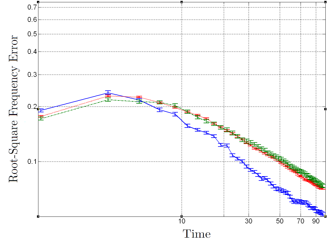
(a)  Root-Square Frequency Error

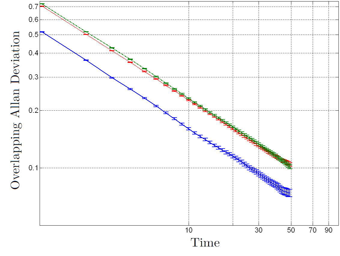
(b)   Overlapping Allan Deviation

Figure 2: A comparison of our protocol (bottom blue solid line), the standard Ramsey protocol (middle red dotted line), and Buzek’s protocol Bužek et al. (1999) (top green dashed line) on a two atom clock subject to standard Brownian motion with $h_{-2}=.03$. We fix the length of the interrogation to $T=1$. Figure (a) is a log-log plot of the root-square error of the frequency averaged over cumulative time, while (b) is a log-log plot of the overlapping Allan deviation with respect to $m$. These are computed with $200$ runs of our method and $1000$ of each of Ramsey’s and Buzek’s protocol.

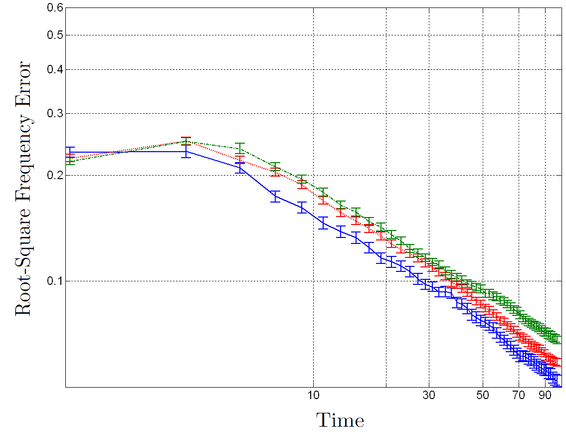
(a)  Root-Square Frequency Error

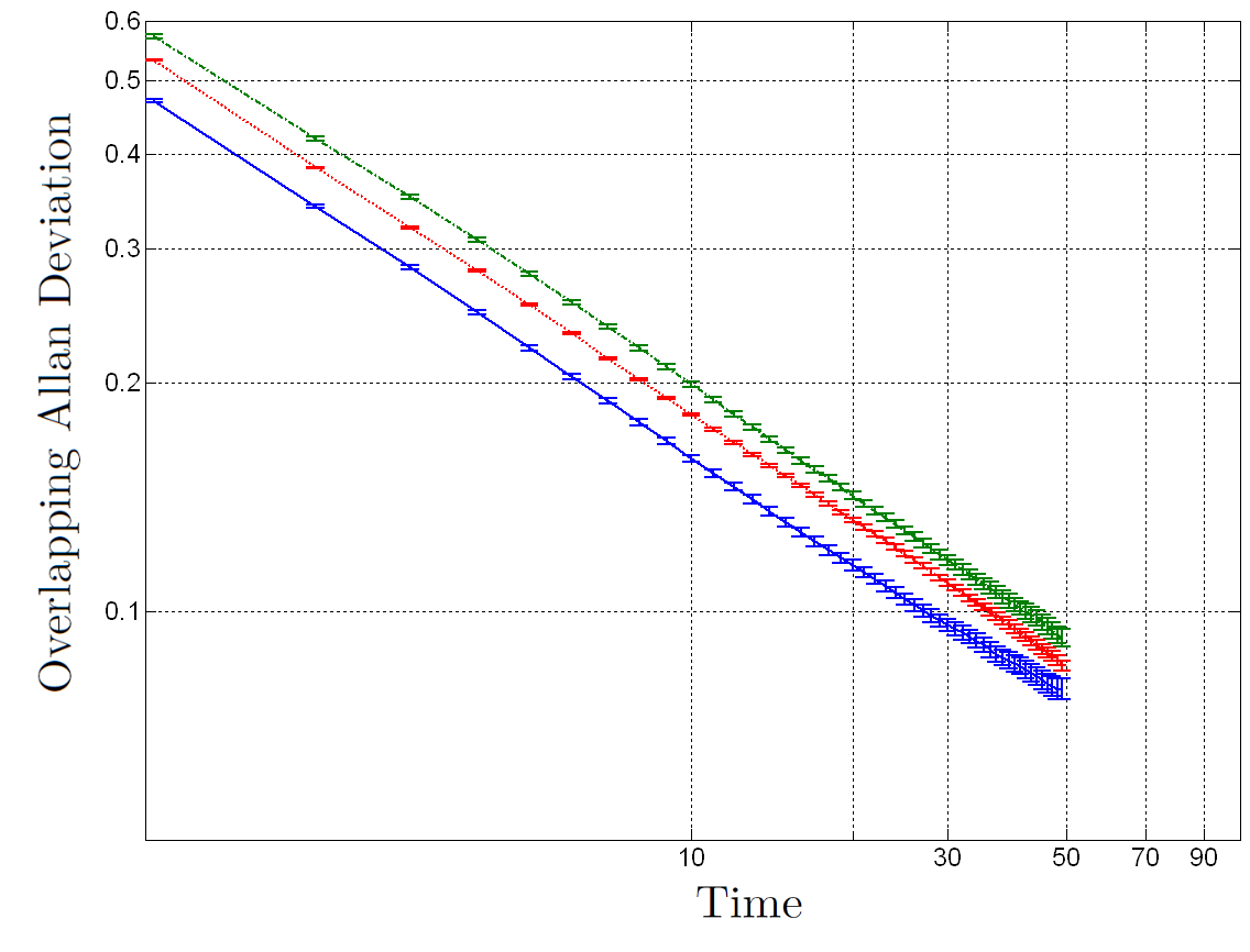
(b)   Overlapping Allan Deviation

Figure 3: A comparison of our protocol (bottom blue solid line), the standard Ramsey protocol (middle red dotted line), and Buzek’s protocol (top green dashed line) on a three atom clock subject to $1/\omega$ noise with $h_{-1}=.05$. Plots (a) and (b) are as described in Fig. 2 and are computed via $400$ iterations of our protocol and $800$ iterations of each of Ramsey’s and Buzek’s protocols.

Noise Type		Ramsey	Buzek
Brownian	Square Error	$46.9\pm.51$	$51.7\pm.46$
Brownian	Allan Variance	$49.3\pm.43$	$50.9\pm.42$
$1/f$	Square Error	$18.9\pm.40$	$39.8\pm.38$
$1/f$	Allan Variance	$21.6\pm.55$	$33.0\pm.48$

Table 1: Percent improvement of our protocol over those of Ramsey and Buzek. We average the gains in square error over the last twenty timesteps and those in Allan variance across all averaging times.

VII Conclusion

While the protocols discussed here already significantly outperform traditional clock protocols, we can obtain further improvements by choosing the interrogation duration $T$ optimally at every step. Longer interrogation durations can provide more information, but if $T$ is chosen too large the clock’s frequency can slip. While this issue is beyond the scope of this paper, we believe our protocol can be adjusted to choose $T$ adaptively. Also, while our protocol performs well even when used with a significantly truncated frequency history, additional storage would, nonetheless, be advantageous. Unfortunately, this often requires a dramatic increase in computation time. It will be helpful to investigate this tradeoff in more detail, and ideally, develop a systematic way to determine when to cut off the clock’s history.

The protocols we have developed were implemented on simulated clocks as a proof-of-principle. Application to an experimental setting requires that the interrogation algorithms obtained be converted to the elementary quantum control operations actually available. Since the interrogation algorithms are different for each timestep, they need to be converted to atom-control operations on the fly. The conversion should optimize control-related decoherence, accuracy of the implemented evolutions, and time. This seems feasible for small numbers of atoms in a sufficiently controllable setting. For more atoms, the optimal interrogation algorithms obtained may be too complex to be implemented with sufficiently low error. It will be necessary to optimize the interrogations in view of limited experimental resources. In practice, it is possible that most of the gains achieved by the protocols can be realized with a restricted set of pre-optimized interrogation algorithms. The effects of the necessary compromises on clock performance need to be investigated.

We conclude by noting that some of the most accurate clocks now being developed use a small number of ions Diddams et al. (2004); Chou et al. (2010). Full quantum control over systems of comparable size has already been demonstrated in ion traps Hanneke et al. (2009). We therefore expect quantum techniques to be experimentally applicable relatively soon. This is in contrast to other domains in which quantum algorithms have been theoretically shown to offer advantages, but where solving useful instances of interesting problems requires control over quantum systems of sizes far beyond what is currently achievable experimentally. Indeed, clocks may be among the first systems where a nontrivial quantum algorithmic gain is realized.

Appendix A Cost Function

To simplify the notation, in the following theorem we write $\theta=\theta_{n-1}$, $a=a_{n}$ and suppress the conditioning on earlier measurement outcomes.

Theorem 1.

Consider a fixed interrogation duration $T$ and use measurement outcomes with labels $a$ denoting arbitrary frequencies. An ideal SDP with the cost function $C=(\omega T-a)^{2}+2(\omega T-a)\mathbf{E}(\theta-\mathbf{E}(\theta)|\omega)$ achieves the minimum expected posterior variance increase of the cumulative phase $\Delta V=\sum_{a}\mathbf{V}(\theta+\omega T|a)p(a)-\mathbf{V}(\theta)$.

Ref. Mullan and Knill (2012) shows that it makes sense to talk about such an ideal SDP, and that the objective values of its discretizations converge to the ideal SDP’s value. The discretization errors are well behaved and can be effectively estimated.

Proof.

For now, we consider fixed algorithms $\mathcal{A}$ and do not identify measurement outcome labels with frequencies. For clarity, we express integrals over measurement outcomes as discrete sums. Consider the expression for $\Delta V$ and expand it as follows:

$$\begin{array}[b]{rl@{}l}\Delta V&=\hbox to0.0pt{$\displaystyle\sum_{a}\mathbf{V}(\theta+\omega T|a)p(a)-\mathbf{V}(\theta)$\hss}&\\ &=\displaystyle\sum_{a}\int\int&\left(\theta^{\prime}+\omega^{\prime}T-\mathbf{E}\left(\theta+\omega T|a\right)\right)^{2}\\ &&p(\theta^{\prime},\omega^{\prime}|a)p(a)d\omega^{\prime}d\theta^{\prime}-\mathbf{V}(\theta).\end{array}$$ (12)

Since, in general,

$$\operatornamewithlimits{argmin}_{y}\mathbf{E}\left(\left(X-y\right)^{2}\right)=\mathbf{V}(X),$$ (13)

we can rewrite Eq. (12) as

$$\begin{array}[b]{rl@{}l}\Delta V&=\displaystyle\min_{g}\sum_{a}\int\int&\left(\theta^{\prime}+\omega^{\prime}T-g(a)\right)^{2}\\ &&p(\theta^{\prime},\omega^{\prime}|a)p(a)d\omega^{\prime}d\theta^{\prime}-\mathbf{V}(\theta),\end{array}$$ (14)

where the minimum is over all functions $g$ of measurement outcomes. We can subtract any constant from inside the square of Eq. (14) without changing its value, as any constant shift will get absorbed in the minimum over $g$. We choose to subtract the constant $\mathbf{E}(\theta)$, yielding

$$\begin{array}[b]{rl@{}l}\Delta V&=\displaystyle\min_{g}\sum_{a}\int\int&\left(\theta^{\prime}-\mathbf{E}\left(\theta\right)+\omega^{\prime}T-g(a)\right)^{2}\\ &&p(\theta^{\prime},\omega^{\prime}|a)p(a)d\omega^{\prime}d\theta^{\prime}-\mathbf{V}(\theta).\end{array}$$ (15)

Expanding the square gives

$$\begin{array}[b]{rl@{}l}\Delta V&=\displaystyle\min_{g}\sum_{a}\int\int\Big{(}&\left(\theta^{\prime}-\mathbf{E}\left(\theta\right)\right)^{2}\\ &&{}+\left(\omega^{\prime}T-g(a)\right)^{2}\\ &&{}+2(\theta^{\prime}-\mathbf{E}\left(\theta\right))\left(\omega^{\prime}T-g(a)\right)\Big{)}\\ &&p(\theta^{\prime},\omega^{\prime}|a)p(a)d\omega^{\prime}d\theta^{\prime}-\mathbf{V}(\theta).\end{array}$$ (16)

Integrating out $\omega^{\prime}$ in the first term gives a summand of $\mathbf{V}(\theta)$ that cancels the subtracted $\mathbf{V}(\theta)$. We can then factor $p(\theta^{\prime},\omega^{\prime}|a)=p(\theta^{\prime}|\omega^{\prime},a)p(\omega^{\prime}|a)$. We know that $\theta^{\prime}$ is conditionally independent of $a$ given $\omega^{\prime}$, that is $p(\theta^{\prime}|\omega^{\prime},a)=p(\theta^{\prime}|\omega^{\prime})$, since $a$’s distribution is completely determined by $\omega^{\prime}$ and the algorithm. We can therefore rewrite Eq. (15) as

$$\begin{array}[b]{rll@{}l}\Delta V&=&\displaystyle\min_{g}\sum_{a}\int&\bigg{(}\displaystyle\int\left(\omega^{\prime}T-g(a)\right)^{2}p(\theta^{\prime}|\omega^{\prime})d\theta^{\prime}\\ &\hbox to0.0pt{$\displaystyle{}+2\left(\omega^{\prime}T-g(a)\right)\int\left(\theta^{\prime}-\mathbf{E}\left(\theta\right)\bigg{)}p(\theta^{\prime}|\omega^{\prime})d\theta^{\prime}\right)$\hss}\\ &&&p(\omega^{\prime}|a)p(a)d\omega^{\prime}.\end{array}$$ (17)

We carry out the integral over $\theta^{\prime}$ and obtain

$$\begin{array}[b]{l}\Delta V=\displaystyle\min_{g}\sum_{a}\int\\ \displaystyle\left(\left(\omega^{\prime}T-g(a)\right)^{2}+2\left(\omega^{\prime}T-g(a)\right)\mathbf{E}\left(\theta-\mathbf{E}\left(\theta\right)|\omega^{\prime}\right)\right)\\ \hphantom{\Delta V=\displaystyle\min_{g}\sum_{a}\int}p(\omega^{\prime},a)d\omega^{\prime}.\end{array}$$ (18)

Define $\bar{C}(g,\mathcal{A})$ to be the expression minimized over $g$ in this identity. It is of the form required by Eq. (6) for the cost function $C$ of the theorem. Here, $\mathcal{A}$ denotes the previously implicit algorithm used for the interrogation. The SDP for $C$ optimizes $\bar{C}(g,\mathcal{A})$ for a fixed $g$ over choices for $\mathcal{A}$. Its objective value is therefore an upper bound on $\Delta V$ for the algorithm found.

Consider now the ideal SDP where the outcomes $a$ are arbitrary frequencies and $g(a)=a$. The optimization over $g$ is now redundant, because this SDP can realize any $\bar{C}(g,\mathcal{A})$ by relabeling the measurement outcomes. Thus, its objective value is the minimum variance increase. ∎

If we consider a discretized version of the SDP in the theorem with fixed $g$, from Eqs. (12), (13) and (14) we deduce that $\Delta V$ for the SDP’s algorithm $\mathcal{A}$ can be computed by replacing $g$ with $g^{\prime}$ defined by $g^{\prime}(a)=\mathbf{E}(\theta+\omega T|a)$ in the expression for $\bar{C}$. Since $\bar{C}(g^{\prime},\mathcal{A})\leq\bar{C}(g,\mathcal{A})$, one can re-evaluate the SDP with $g^{\prime}$ in place of $g$. Iterating this procedure in the limit yields an algorithm for which $g=g^{\prime}$. Whether the resulting algorithm achieves the optimal $\Delta V$ may depend on the starting choices and the number of measurement outcome labels. But the bounds on discretization error from Ref. Mullan and Knill (2012) guarantee that the solution can be made arbitrarily close to optimal.

Observe that the two terms of Eq. (18) resemble $\mathbf{V}(\omega T)$ and $2\mathbf{Cov}(\omega T,\theta)$, respectively, except that for the optimal choice of $g$, the offset for $\omega T$ is not its mean. The dependence of the second term on $\mathbf{E}(\theta|\omega)$ prevents the cost from being a simple quadratic.

Appendix B Conditional Multivariate Gaussians

For the noise models used here, the prior distribution $p(\omega_{1},\omega_{2}\ldots\omega_{N})\equiv p(\bm{\omega_{N}})$ is a multivariate Gaussian with means given by $\bm{\mu}=(\mathbf{E}(\omega_{1}),\mathbf{E}(\omega_{2}),\ldots\mathbf{E}(\omega_{N}))$ and covariance matrix $\bm{C}_{i,j}=\mathbf{Cov}(\omega_{i},\omega_{j})$. These means and covariances completely characterize the distribution. The clock updates require computing $p(\omega_{N}|\bm{\omega_{N-1}})$. This conditional probability distribution is also Gaussian and it suffices to compute its mean and variance. Denote the submatrix of $\bm{C}$ containing rows $r$ through $s$ and columns $c$ through $d$ as $\bm{C}_{[r,s],[c,d]}$, and define subvectors $\bm{\mu}_{[r,s]}$ of $\bm{\mu}$ in the same way. The desired mean is given by Eaton and Eaton (1983)

$$\mu^{\prime}=\mu_{N}+\bm{C}_{N,[1,N-1]}\bm{C}_{[1,N-1],[1,N-1]}^{-1}(\bm{f}-\bm{\mu}_{[1,N-1]}),$$ (19)

and the variance by

$$C^{\prime}=C_{N,N}-\bm{C}_{N,[1,N-1]}\bm{C}_{[1,N-1],[1,N-1]}^{-1}\bm{C}_{[1,N-1],N}.$$ (20)

Appendix C Expectation Updates

Before we can obtain the quantum algorithm for the next interrogation, it is necessary to compute the parameters of the cost-function of Eq. (7). These parameters depend on conditional expectations of $\theta_{n}$. Because $\theta_{n}$ depends on all frequencies since the clock was started, it is not clear how to compute these expectations when the history is truncated to keep the memory requirements manageable. Here we show that the relevant expectations can be updated correctly with respect to the noise model implied by the truncation strategy and without requiring additional distributions to be maintained.

Truncation converts the ideal noise model into one with finite memory as far as the frequencies $\omega_{n}$ are concerned. The prior distribution for $\omega_{n+1}$ is computed taking into account only its covariances with $\omega_{n},\ldots,\omega_{n-m+1}$, where the history is truncated after $m$ interrogations. The truncated noise model satisfies that $\omega_{n+1}$ is conditionally independent of $\omega_{l}$ for $l<n-m+1$ given $\omega_{n},\ldots,\omega_{n-m+1}$. Here we consider the more general situation, where the relevant state of the oscillator after the $n$’th interrogation is parameterized by $s_{n}$. For the truncated history and resulting noise models used here, $s_{n}=(\omega_{n},\ldots,\omega_{n-m+1})$. Given this setup and the accordingly modified (though not ideal) noise model, we can ensure that the distributions of $\omega_{n+k}$ ($k>0$) are conditionally independent of $s_{n-l}$ ($l>0$) and $\theta_{n}$ given $s_{n}$ and $\mathbf{a}_{n}$. We also assume that the values of all the relevant random variables have been discretized, so that integrals are replaced by sums.

We now show how to keep track of the conditional moments $M_{k,n}=\mathbf{E}(\theta_{n}^{k}|s_{n},\bm{a_{n}})$ for $k\leq K$ as we update the various conditional distributions needed to compute priors and posteriors. The cost function needed to optimize the $n{+}1$’th interrogation requires the expectations $\mathbf{E}(\theta_{n}|\omega_{n+1},\mathbf{a}_{n})$ and $\mathbf{E}(\theta_{n}|\mathbf{a}_{n})$. The second can be obtained from the first by integrating over $\omega_{n+1}$ with respect to the distribution $p(\omega_{n+1}|\mathbf{a}_{n})=\sum_{s_{n}}p(\omega_{n+1}|s_{n},\mathbf{a}_{n})p(s_{n}|\mathbf{a}_{n})$. These conditional distributions are available and updated by the protocol after each interrogation. Given $M_{1,n}$, the first expectation can be computed by setting $k=1$ in the following:

$$\begin{array}[b]{l}\displaystyle\mathbf{E}(\theta_{n}^{k}|\omega_{n+1},\bm{a_{n}})\\ \displaystyle\quad{}=\sum_{s_{n}}\mathbf{E}(\theta_{n}^{k}|\omega_{n+1},s_{n},\bm{a_{n}})p(s_{n}|\omega_{n+1},\bm{a_{n}})\\ \displaystyle\quad{}=\sum_{s_{n},\theta_{n}}\theta_{n}^{k}p(\theta_{n}^{k}|\omega_{n+1},s_{n},\bm{a_{n}})p(s_{n}|\omega_{n+1},\bm{a_{n}})\\ \displaystyle\quad{}=\sum_{s_{n},\theta_{n}}\theta_{n}^{k}p(\theta_{n}^{k}|s_{n},\bm{a_{n}})p(s_{n}|\omega_{n+1},\bm{a_{n}})\\ \displaystyle\quad{}=\sum_{s_{n}}\mathbf{E}(\theta_{n}^{k}|s_{n},\bm{a_{n}})p(s_{n}|\omega_{n+1},\bm{a_{n}})\\ \displaystyle\quad{}=\sum_{s_{n}}M_{k,n}p(s_{n}|\omega_{n+1},\bm{a_{n}}).\end{array}$$

In the third identity we applied the conditional independence of $\omega_{n+1}$ and $\theta_{n}$ given $s_{n}$ and $\mathbf{a}_{n}$. The factor in the last sum is determined by the noise model and is available to the protocol. We observe that the mean-square-errors needed for evaluating protocol performance can be obtained from the second moments ($k=2$) without the need for a full Monte Carlo simulation.

For computing $M_{k,n+1}$ from the $M_{k^{\prime},n}$, we are given $p(s_{n}|\bm{a_{n}})$ and can compute $p(\omega_{n+1},s_{n}|\bm{a_{n}})$ and all derived conditionals and marginals. At this point we also know the outcome $a_{n+1}$. Expand $M_{k,n+1}$ as follows:

$$\begin{array}[b]{l}\displaystyle\mathbf{E}(\theta_{n+1}^{k}|s_{n+1},\bm{a_{n+1}})\\ \displaystyle\quad{}=\mathbf{E}\left(\left(\theta_{n}+\omega_{n+1}T_{n+1}\right)^{k}|s_{n+1},\bm{a_{n+1}}\right)\\ \displaystyle\quad{}=\sum_{j=0}^{k}\mathbf{E}\left({k\choose j}T_{n+1}^{j}\omega_{n+1}^{j}\theta_{n}^{k-j}|s_{n+1},\bm{a_{n+1}}\right).\end{array}$$ (21)

To evaluate the $j$’th term of this sum we can compute

$$\begin{array}[b]{l}\displaystyle\mathbf{E}(\omega_{n+1}^{j}T^{j}_{n+1}\theta_{n}^{k-j}|s_{n+1},\bm{a_{n+1}})\\ \displaystyle\quad{}=\sum_{\omega_{n+1}}\omega_{n+1}^{j}T^{j}_{n+1}\mathbf{E}(\theta_{n}^{k-j}|\omega_{n+1},s_{n+1},\bm{a_{n+1}})\\ \displaystyle\hphantom{\quad{}={}\sum_{\omega_{n+1}}\omega_{n+1}^{j}T^{j}_{n+1}}\times p(\omega_{n+1}|s_{n+1},\bm{a_{n+1}}).\end{array}$$ (22)

We have that $\theta_{n}$ is conditionally independent of $\omega_{n+1}$, $s_{n+1}$, and $a_{n+1}$ given $s_{n}$ and $\bm{a}_{n}$. Therefore,

$$\begin{array}[b]{l}\displaystyle\mathbf{E}(\theta_{n}^{k-j}|\omega_{n+1},s_{n+1},\bm{a_{n+1}})\\ \displaystyle\quad{}=\sum_{s_{n}}\mathbf{E}(\theta_{n}^{k-j}|\omega_{n+1},s_{n+1},s_{n},\bm{a_{n+1}})\\ \displaystyle\phantom{\quad{}=\sum_{s_{n}}\mathbf{E}(\theta_{n}^{k-j}|}\times p(s_{n}|\omega_{n+1},s_{n+1},\bm{a_{n+1}})\\ \displaystyle\quad{}=\sum_{s_{n}}\mathbf{E}(\theta_{n}^{k-j}|s_{n},\bm{a_{n}})p(s_{n}|\omega_{n+1},s_{n+1},\bm{a_{n+1}})\\ \displaystyle\quad{}=\sum_{s_{n}}M_{k-j,n}p(s_{n}|\omega_{n+1},s_{n+1},\bm{a_{n+1}}).\end{array}$$ (23)

The last factor in the summand is determined by the noise model and the algorithm used for the $n+1$’th interrogation. It is can therefore be computed from the posteriors maintained by the protocol.

Appendix D Timing Error Suppression

We describe methods for suppressing the errors due to differences between $T_{n}$ and the true interrogation duration determined from the external oscillator, and the errors from non-instantaneous state preparation and measurement. We argue that with proper implementation design, uncertainties in these durations are a small fraction of the intended interrogation duration $T$, which results in relatively small biases when inferring external oscillator frequencies. This requires that the change in actual interrogation duration does not significantly affect the noise accumulated according to the noise model and that there is little change in the conditional probability distributions of the measurement outcomes given the true frequency $\omega$ of the oscillator for the duration of the interrogation. Relative to the accumulated noise for the total interrogation duration $T$, the contribution associated with differences between $T$ and the effective interrogation duration $T^{\prime}$ relates to $(T-T^{\prime})/T$ with a corresponding small effect on the clock. The conditional probability distributions are determined by the measurement procedure, which our protocol specifies in the frame of the atomic standard at the end of the interrogation period. The implementation must use the frame of the external oscillator instead, so the measurement is adjusted for the experimenter’s best estimate of the relative phases. Because the oscillator is classical, the experimenter has access to the absolute oscillator phase $\phi$ relative to the beginning of the interrogation. This phase relates to the true time difference $s$ according to $\phi=(\omega+\Omega)s$, where, for current purposes, $\omega$ is the true average frequency deviation from $0$ to $s$, and $\Omega$ is the (unchanging) frequency of the atomic standard. The quantum algorithm obtained in the procedure expects that the measurement is at time $s=T$ and the relative phase of the atomic standard compared to the oscillator at this time is $-\omega T$. For $s\not=T$ the actual relative phase is $-\omega s$, which can be substantially different if the oscillator has drifted and the measurement duration is non-negligible. The experimenter can compensate for this issue by modifying the measurement phase in time according to the best estimate $\omega^{*}$ of $\omega$. If $s$ is known, a good compensating phase is $\omega^{*}(s-T)$, and with this compensation, the phase error is reduced to $\epsilon=(\omega^{*}-\omega)(s-T)$, so the measurement is not sensitive to long term drift of the oscillator. Note that this procedure is equivalent to offsetting the oscillator frequency by $-\omega^{*}$, which corresponds to the standard practice of controlling the oscillator to stay close to the atomic standard. To avoid having to modify our noise model and representations of probability distributions, we find it convenient to perform this control in software instead.

The above compensating phase $\omega^{*}(s-T)$ cannot be used directly since $s$ is not known. The experimenter’s best estimate for $s$ is $s^{*}=\phi/(\omega^{*}+\Omega)$. If this is used, the compensating phase at the time of measurement is $\omega^{*}(s^{*}-T)$, or $\phi\,\omega^{*}/(\omega^{*}+\Omega)-\omega^{*}T$ in terms of the external oscillator phase $\phi$. The phase error is

$$\epsilon =-\omega T-(-\omega s+\omega^{*}(s^{*}-T))$$

$$=(\omega^{*}-\omega)(T-s)+\omega^{*}(s-s^{*})$$

$$=(\omega^{*}-\omega)(T-s)+\omega^{*}s\left(1-\frac{\omega+\Omega}{\omega^{*}+\Omega}\right)$$

$$=(\omega^{*}-\omega)\left((T-s)+\frac{\omega^{*}}{\omega^{*}+\Omega}s\right).$$ (24)

To avoid phase slip, it is necessary to choose $T$ such that $(\omega^{*}-\omega)T<\pi$ with high probability. If this inequality holds, then the phase error is bounded by

$$E_{1}=\pi|T-s|/T+\pi(s/T)(\omega^{*}/(\omega^{*}+\Omega)),$$ (25)

both of which are expected to be small. Furthermore, even without controlling the oscillator to avoid large excursions, we expect the first term to dominate.

To avoid problems from finite preparation and measurement durations, the compensating phase must be applied continuously in time. A direct way to do this is by providing an auxilliary oscillator locked to the external oscillator and offset by $-\omega^{*}$. Specifically, the phase of the auxilliary oscillator is given by $-\phi\omega^{*}/(\omega^{*}+\Omega)$ with respect to the phase $\phi$ of the external oscillator. For state preparation, operations applied to the atom have phase $0$ with respect to the auxilliary oscillator. For measurement, the phase with respect to the auxilliary oscillator and added to the phases of the measurement computed by the SDP is given by $T\omega^{*}$. The measurement period is centered around the time when the phase of the external oscillator is $\phi=T(\omega^{*}+\Omega)$. With this procedure, the error due to preparation and measurement durations of order $\Delta T$ is directly related to the phase error due to non-ideal true measurement durations of the same order.

Large excursions of $\omega$ compared to $\Omega$ are not normally expected. Nevertheless, it may be desirable to eliminate the second term contributing to the phase error in Eq. (25). For this purpose, one can modify the SDP used to compute the optimal protocol. If the experimenter determines the end of the interrogation according to $\phi_{T}=T(\omega^{*}+\Omega)$, the true time at the end is $\phi_{T}/(\omega+\Omega)=T(\omega^{*}+\Omega)/(\omega+\Omega)$. The relative phase is $\rho(\omega)T=\omega T(\omega^{*}+\Omega)/(\omega+\Omega)$ instead of $\omega T$. This changes the relationship between $\omega$ and the phase of the interrogation unitary, since the construction of the SDP as given in the text assumes that the accumulated phase difference is $-\omega T$. The modified phase difference can be accommodated by a re-parameterization of the frequencies in the SDP. This is accomplished by defining $\omega^{\prime}=\rho(\omega)$, computing the prior needed by the SDP for $\omega^{\prime}$ from that for $\omega$ accordingly and using the cost function $C^{\prime}$ defined by $C^{\prime}(\omega^{\prime},a)=C(\rho^{-1}(\omega^{\prime}),a)$ in Eq. (6). The continuously applied measurement phase compensation to account for the non-instantaneous and inexact measurement is then given by $(\phi-\phi_{T})\omega^{*}/(\omega^{*}+\Omega)$ as a function of the oscillator phase $\phi$, which is identical to that given by the earlier method that simulates a locked oscillator, previously expressed as $\phi\omega^{*}/(\omega^{*}+\Omega)-\omega^{*}T$. With the reparametrized cost function and this phase compensation, the remaining phase error compared to protocol expectation is given by

$$\epsilon =(\phi-\phi_{T})\left(\frac{\omega}{\omega+\Omega}-\frac{\omega^{*}}{\omega^{*}+\Omega}\right)$$

$$=(\omega-\omega^{*})\frac{\phi-\phi_{T}}{\omega+\Omega}\;\frac{\Omega}{\omega^{*}+\Omega}.$$ (26)

To explicitly compare this to the earlier error, note that $s-T=(\phi-\phi_{T})/(\omega+\Omega)$ corresponds to the difference between the ideal interrogation duration and the implemented one, and $(\omega-\omega^{*})T<\pi$, so the error is bounded by $\pi(|T-s|/T)\Omega/(\omega^{*}+\Omega)$. This is expected to be small but shows that low absolute oscillator frequencies require correspondingly more precise interrogation durations. Note that in general, low-frequency oscillators do not make good clocks and real noise models are not frequency independent.

References

- Wineland et al. (1992) D. Wineland, J. Bollinger, W. Itano, F. Moore, and D. Heinzen, Physical Review A 46, 6797 (1992).
- Kitagawa and Ueda (1993) M. Kitagawa and M. Ueda, Physical review. A 47, 5138 (1993).
- Wineland et al. (1994) D. Wineland, J. Bollinger, W. Itano, and D. Heinzen, Physical Review A 50, 67 (1994).
- Bollinger et al. (1996) J. J. Bollinger, W. M. Itano, D. J. Wineland, and D. J. Heinzen, Phys. Rev. A 54, R4649 (1996).
- Huelga et al. (1997) S. Huelga, C. Macchiavello, T. Pellizzari, A. Ekert, M. Plenio, and J. Cirac, Phys. Rev. Lett. 79, 3865 (1997).
- Berry et al. (2009) D. Berry, B. Higgins, S. Bartlett, M. Mitchell, G. Pryde, and H. Wiseman, Physical Review A 80, 052114 (2009).
- Higgins et al. (2007) B. Higgins, D. Berry, S. Bartlett, H. Wiseman, and G. Pryde, Nature 450, 393 (2007).
- Huver et al. (2008) S. D. Huver, C. F. Wildfeuer, and J. P. Dowling, Phys. Rev. A 78, 063828 (2008), URL http://link.aps.org/doi/10.1103/PhysRevA.78.063828.
- Luis (2002) A. Luis, Phys. Rev. A 65, 025802 (2002), URL http://link.aps.org/doi/10.1103/PhysRevA.65.025802.
- Dorner (2012) U. Dorner, New Journal of Physics 14, 043011 (2012).
- Dorner et al. (2009) U. Dorner, R. Demkowicz-Dobrzanski, B. J. Smith, J. S. Lundeen, W. Wasilewski, K. Banaszek, and I. A. Walmsley, Phys. Rev. Lett. 102, 040403 (2009), URL http://link.aps.org/doi/10.1103/PhysRevLett.102.040403.
- Wineland et al. (1998) D. J. Wineland, C. Monroe, W. M. Itano, D. Leibfried, B. E. King, and D. M. Meekhof, J. Res. NIST 103, 259 (1998).
- André et al. (2004) A. André, A. S. Sørensen, and M. D. Lukin, Phys. Rev. Lett. 92, 230801 (2004).
- Bužek et al. (1999) V. Bužek, R. Derka, and S. Massar, Phys. Rev. Lett. 82, 2207 (1999), eprint arXiv:quant-ph/9808042.
- Demkowicz-Dobrzański (2011) R. Demkowicz-Dobrzański, Phys. Rev. A 83, 061802 (2011), URL http://link.aps.org/doi/10.1103/PhysRevA.83.061802.
- van Dam et al. (2007) W. van Dam, G. D Ariano, A. Ekert, C. Macchiavello, and M. Mosca, Phy. Rev. Lett. 98, 90501 (2007).
- Macieszczak et al. (2013) K. Macieszczak, R. Demkowicz-Dobrzanski, and M. Fraas, arXiv preprint arXiv:1311.5576 (2013).
- Rosenband (2012) T. Rosenband (2012), arXiv:1203.0288v2.
- Giovannetti et al. (2011) V. Giovannetti, S. Lloyd, and L. Maccone, Nat. Phot. 5, 222 (2011).
- Mullan and Knill (2012) M. Mullan and E. Knill, Quantum Information and Computation 12, 553 (2012).
- Allan (1966) D. Allan, Proceedings of the IEEE 54, 221 (1966), ISSN 0018-9219.
- Riley (2008) W. J. Riley, Handbook of Frequency Stability Analysis, vol. NIST Special Publication 1065 (NIST, Boulder, CO, 2008).
- Numata et al. (2004) K. Numata, A. Kemery, and J. Camp, Phys. Rev. Lett. 93, 250602 (2004), URL http://link.aps.org/doi/10.1103/PhysRevLett.93.250602.
- Fyodorov et al. (2009) Y. V. Fyodorov, P. L. Doussal, and A. Rosso, Journal of Statistical Mechanics: Theory and Experiment 2009, P10005 (2009), URL http://stacks.iop.org/1742-5468/2009/i=10/a=P10005.
- Diddams et al. (2004) S. A. Diddams, J. C. Bergquist, S. R. Jefferts, and C. W. Oates, Science 306, 1318 (2004), eprint http://www.sciencemag.org/content/306/5700/1318.full.pdf, URL http://www.sciencemag.org/content/306/5700/1318.abstract.
- Chou et al. (2010) C. W. Chou, D. B. Hume, J. C. J. Koelemeij, D. J. Wineland, and T. Rosenband, Phys. Rev. Lett. 104, 070802 (2010), URL http://link.aps.org/doi/10.1103/PhysRevLett.104.070802.
- Hanneke et al. (2009) D. Hanneke, J. P. Home, J. D. Jost, J. M. Amini, D. Leibfried, and D. J. Wineland, Nature Physics 6, 13 (2009).
- Eaton and Eaton (1983) M. L. Eaton and M. Eaton, Multivariate statistics: a vector space approach (Wiley New York, 1983).