Final state interaction in $D^{+}\to K^{-}\pi^{+}\pi^{+}$ with $K\pi$ I=1/2 and 3/2 channels

Abstract

The final state interaction contribution to $D^{+}$ decays is computed for the $K^{-}\pi^{+}\pi^{+}$ channel within a light-front relativistic three-body model for the final state interaction. The rescattering process between the kaon and two pions in the decay channel is considered. The off-shell decay amplitude is a solution of a four-dimensional Bethe-Salpeter equation, which is decomposed in a Faddeev form. The projection onto the light-front of the coupled set of integral equations is performed via a quasi-potential approach. The S-wave $K\pi$ interaction is introduced in the resonant isospin $1/2$ and the non-resonant isospin $3/2$ channels. The numerical solution of the light-front tridimensional inhomogeneous integral equations for the Faddeev components of the decay amplitude is performed perturbatively. The loop-expansion converges fast, and the three-loop contribution can be neglected in respect to the two-loop results for the practical application. The dependence on the model parameters in respect to the input amplitude at the partonic level is exploited and the phase found in the experimental analysis, is fitted with an appropriate choice of the real weights of the isospin components of the partonic amplitude. The data suggests a small mixture of total isospin $5/2$ to the dominant $3/2$ one. The modulus of the unsymmetrized decay amplitude, which presents a deep valley and a following increase for $K\pi$ masses above $1.5$ GeV, is fairly reproduced. This suggests the assignment of the quantum numbers $0^{+}$ to the isospin 1/2 $K^{*}(1630)$ resonance.

I Introduction

Weak decays of heavy flavoured hadrons provide unique opportunities to probe the interplay of the electroweak theory and Quantum Chromodynamics (QCD). The weak part of these decays involve short-distance transitions at the quark-level, whereas the hadron formation is governed by the long-distance, low-energy strong interactions.

Due to the non-perturbative character of the strong interactions involved in heavy flavour decays, the hadronization is not calculable from first principles. In the kaon sector, chiral perturbation methods are applicable, given the small value of the $s$ quark mass. In the opposite extreme, the mass of the $b$ quark is heavy enough to allow for reliable calculations based on effective field theories. The charm quark is in between these two cases, which makes the computation of decay rates a challenging task.

The study of the Charge-Parity (CP) violation CPV1 ; CPV2 is an important example where the hadronic part of the decay amplitude needs to be quantitatively understood. CP) violation is phenomenon where manifestations of new physics are expected. In the Standard Model (SM), CP violation processes are related to the complex phase in Cabibbo-Kobayashi-Maskawa matrix (CKM) CKM1 ; CKM2 , which describes the mixture between different generations of quarks. SM predicts very small CP violation effects in charm decays, in spite of large uncertainties. This makes charm decays a very interesting place to search for new sources of CP violation. New physics would introduce additional CP-violating phases, but disentangling these from the SM CP violation require the control of the overwhelming strong phases.

We emphasize the advantages of the experimental investigation of the three-body charm meson decays. These decays are, in general, dominated by resonant intermediate states, with a small non-resonant component Bianco . With three-body decays one can search for local CP violation effects, but the description of the decay dynamics requires the understanding of hadronic effects such as the three-body final state interactions and the role of the S-wave component.

In this paper we address the issue of three-body final state interactions (FSI) in the decay $D^{+}\rightarrow K^{-}\pi^{+}\pi^{+}$, with emphasis on the S-wave component of the $K^{-}\pi^{+}$ amplitude. This channel is chosen for several reasons: it is abundant, being studied by different experiments like E791 Aitala12 ; Aitala3 , FOCUS FOCUS1 ; FOCUS2 and CLEO CLEO ; it has a dominant S-wave component and a small non-resonant amplitude; it allows the continuously study of the $K\pi$ S-wave amplitude from threshold, at $633$ MeV/c², up to $1.7$ GeV/c², covering the whole elastic regime. With the $D^{+}\rightarrow K^{-}\pi^{+}\pi^{+}$ decay one can fill the gap of the existing data on $K\pi$ scattering from the LASS experiment LASS (LASS data for the $K\pi$ scattering starts only at 825 MeV/c²).

The resonant structure of three-body decays are determined by the analysis of the Dalitz plot Dalitz . In this two-dimensional diagram, the probability density of a pseudo-scalar particle $P$, decaying into three pseudoscalar particles ($d_{1},d_{2},d_{3}$), is given by

$$d\Gamma(P\to d_{1}d_{2}d_{3})\propto\frac{1}{M^{3}_{P}}\,|\mathcal{M}(s_{12},s_{13})|^{2}\,ds_{12}\,ds_{13}$$ (1)

where $M_{P}$ is the mass of the parent particle. The phase-space density, ${M^{-3}_{P}}$, is constant, so the structures reveal the decay dynamics, forming the resonances, which are also affected by final state interactions. The goal of the Dalitz plot analysis is to determine the matrix element $\mathcal{M}(s_{12},s_{13})$.

The Dalitz plot analysis of the $D^{+}\rightarrow K^{-}\pi^{+}\pi^{+}$ was performed by different experiments, such as MARK III Adler1987a ; Adler1987b ; Adler1987c ; Adler1987d , NA14 Alvarez ; Alvarez2 , E691 Anjos ; Anjos2 , E687 Frabetti ; Frabetti2 , E791Aitala12 and FOCUS FOCUS1 ; FOCUS2 , using different decay models. These decay models differ in the way the S-wave is described: the sum of Breit-Wigners plus a constant nonresonant term, refered to as the Isobar Model, the K-matrix formalism and a model independent partial wave analysis (MIPWA), to which we give special attention.

The MIPWA technique, developed by E791 Aitala2006 , is intended to extract, in a independent way, the S-wave $K\pi$ amplitude of the $D^{+}\rightarrow K^{-}\pi^{+}\pi^{+}$ decay. In the MIPWA, the S-wave $K\pi$ amplitude is a generic function, $A_{0}(s)=a_{0}e^{i\phi_{0}(s)}$, given by the fit of the Dalitz plot. The P and D wave are determined according the Isobar Model. Although the MIPWA is the most model-independent approach, the extraction of the phase is an inclusive measurement, comprising different isospin amplitudes and FSI.

As a matter of fact, the comparison between the S-wave from scattering and from $D$ decays show important differences which need to be understood. In addition to an overall shift of approximately 150 degrees, the two amplitudes have different shapes.

The S-wave $K\pi$ amplitude depends on the isospin and orbital angular momentum of the system. There are two isospin states possible for this system, namely, $I=1/2$ and $I=3/2$. In the case of the LASS experiment, it was shown that resonances and the corresponding scattering amplitude poles are present only in the isospin 1/2 channel, as verified in the analysis of the phase $\delta_{I=1/2}(m_{K\pi})$ Alberto . It is expected that this phase would be common to all processes having a $K\pi$ system, in the absence of rescattering involving other particles in the final state. This should be valid to all angular momentum states, according to the Watson theorem Watson .

The S-wave phase-shift obtained from the $D^{+}\to K^{-}\pi^{+}\pi^{+}$ decay with the MIPWA (FOCUS and E791) differ from that obtained from $K\pi$ scattering (LASS). There is an energy dependent discrepancy that cannot be cured by any combination of $\delta_{I=1/2}$ and $\delta_{I=3/2}$. Indeed, up to an overall shift of $\sim 150^{\circ}$ , such an energy dependence was reproduced quite nicely below $K^{*}_{0}(1430)$ in a chiral three-body model of the $K\pi\pi$ decay with S-wave $K\pi$ interaction, in the resonant isospin $1/2$ channel and computed up to two-loops MagPRD11 . We should mention that a previous attempt BoitoPRD09 ; Boito:2010qe to describe the decay $D^{+}\rightarrow K^{-}\pi^{+}\pi^{+}$ considering only two-body FSI (no 3-body FSIs and factorization of the weak vertex) was also quite successful phenomenologically below $K^{*}_{0}(1430)$.

Our aim is to further explore theoretically the three-body final state interaction in the $D^{+}\rightarrow K^{-}\pi^{+}\pi^{+}$ decay. The motivation of our study is the possibility of three-body rescattering in $D^{+}\rightarrow K^{-}\pi^{+}\pi^{+}$ decay for $K\pi$ interactions in both isospin channels, while fitting the LASS data in the whole kinematical region of the experiment up to $1.89$ GeV. Our study is based in a relativistic model for the three-body final state interaction in $D^{+}\rightarrow K^{-}\pi^{+}\pi^{+}$ decay, starting with the three-meson Bethe-Salpeter equation karinnpb ; pos ; MagPRD11 .

In the model developed here, the decay amplitude is separated into a smooth term and a three-body fully interacting contribution, which is factorized in the standard two-meson resonant amplitude times a reduced complex amplitude for the bachelor meson, that carries the effect of the three-body rescattering mechanism. The off-shell bachelor reduced amplitude is a solution of an inhomogeneous Faddeev type integral equation, that has as input the S-wave isospin $1/2$ and $3/2$ $K^{-}\pi^{+}$ transition matrix. The theoretical contribution of the present work is to use in the three-body rescattering equations the S-wave two-body $K\pi$ amplitude in both isospin states, $1/2$ and $3/2$, fitted up to $1.89$ GeV. We neglect the interaction between the identical charged pions.

The three-body model of the decay amplitude is recasted in a Bethe-Salpeter like equation, which is conveniently rewritten in terms of a Faddeev expansion. The contribution of the final state interaction in the three-body decay of a heavy-meson in our model of the S-wave $K\pi$ transition amplitude is encoded by a bachelor amplitude associated with each Faddeev component of the full decay amplitude. The bachelor function modulates the $K\pi$ scattering amplitude in the final decay channel and in general carries a phase. The advantage of using the Faddeev decomposition of the decay amplitude, is that (i) the integral equation for the bachelor function has a connected kernel, and (ii) the kernel is written in terms of the two-body scattering amplitude directly, instead of the potential. We use a parametrization of the $K\pi$ scattering amplitude in $I=1/2$ and $3/2$, which is input to the bachelor integral equations, and constitutes one source of the energy dependence seen in the $D^{+}\rightarrow K^{-}\pi^{+}\pi^{+}$ S-wave phase shift, besides the phase of the $K\pi$ amplitude. Technically, we perform the light-front projection of the equations sales00 ; MarPRD07 ; MarPoS08 ; MarFBS08 ; MarPRD08 ; FredFBS11 ; FreFBS14 , to simplify the numerical computation of the observables by three-dimensional integrations. These techniques are well exemplified in the reviews of applications of light-front field theory to nuclear and hadron physics Karmanov1 ; brodsky . In particular, we should mention the application of light-front quantization to describe three-body systems, see e.g. BakNPB79 ; FudPRC87 ; FrePLB92 ; AdhAP94 ; CarPRC03 .

The work is organized as follows. In Sec. II, we present our fitting model for the $K\pi$ $I=1/2$ S-wave phase-shift up to about $1.89$ GeV of the LASS data LASS . In the following sections, the relativistic formalism to compute the contribution of three-body final state interaction in heavy-meson decays is developed. In Sec. III, we present the derivation of a covariant and four-dimensional Bethe-Salpeter equation for the three-body decay with rescattering effects. In Sec. IV, we present the light-front projection technique and derive the three-dimensional equations for the bachelor amplitude. In Sec. V, the isospin projection of the LF equations for the bachelor amplitudes derived in the preceding section is performed. The perturbative solution of the LF integral equations are constructed in Sec. VI for the bachelor amplitude up to three-loops, namely, up to terms in third order in the two-body transition matrix to check convergence. In Sec. VII the numerical results for the $D^{+}\rightarrow K^{-}\pi^{+}\pi^{+}$ with three-body final state interaction and $K\pi$ interactions in $I=1/2$ and $3/2$ states are presented. In Sec. VIII, we summarize the main contributions of this work to both the experimental and theoretical analysis of the $D^{+}\rightarrow K^{-}\pi^{+}\pi^{+}$ decay.

II $K\pi$ S-wave amplitude

The S-wave amplitudes of the $K\pi$ elastic scattering in the resonant $I_{K\pi}=1/2$ and the non-resonant one $I_{K\pi}=3/2$ states are the inputs of our model of the $3\to 3$ T-matrix, which brings the final state interaction between the three mesons to the $D^{+}\to K^{-}\pi^{+}\pi^{+}$ decay. As we already mentioned, the interaction of the identical pions is neglected. Here, we just follow karinnpb ; FreFBS14 for the parametrization of the LASS data LASS in the S-wave resonant $I_{K\pi}$=1/2 channel. In addition to the $K^{*}_{0}(1430)$, we use the resonances $K_{0}^{*}(1630)$ (in Particle Data Group PDG there is no assignment of spin to $K(1630)$) and $K_{0}^{*}(1950)$). The lowest resonance and broad one $K_{0}^{*}(800)$ comes with the effective range parameters. In Ref. MagPRD11 , it was the result of the low energy chiral dynamics and unitarity, appearing naturally as a pole in the S-channel.

The motivation to include the higher radial excitations of $K^{*}_{0}$ comes from recent proposal to interpret the scalar meson family ($f_{0}$) as radial excitations of the $\sigma$ meson as proposed in Refs. dePaulaPLB10 ; dePaula:2010yu . This result was obtained by using a Dynamical AdS/QCD modeldePaula:2008fp , where the backreaction between the dilaton field and a deformed anti-de Sitter metric is taken into account. Using a different approach, in MasPRD12 it was also proposed a systematics of radial Regge trajectories for light scalars, which couples these resonances to the $\pi\pi$ channels. By analogy, if these analyses are extended to the strange sector it would suggest a mass spectrum ($M^{2}\times n$) for the kappa family with a rough slope of $\sim 0.6$ GeV², and also the decay of these mesons in the $K\pi$ S-wave $I_{K\pi}=1/2$ channel. The fitting of the LASS data in this isospin channel is the main reason to use more resonances, namely, $K_{0}^{*}(1630)$ and $K_{0}^{*}(1950)$ besides $K_{0}^{*}(1430)$. Being conservative, these further resonances can be considered at the moment as a practical way to fit the data in the whole kinematical range up to $1.89$ GeV.

The parametrization of our relativistic model of the S-wave $I_{K\pi}=1/2$ scattering amplitude extends the one used in Ref. BABAR , where we introduce also $K_{0}^{*}(1630)$ and $K_{0}^{*}(1950)$. The relativistic scattering amplitude as a function of $M^{2}_{K\pi}$ is written in terms of the S-matrix ($S^{\mbox{\tiny{1/2}}}_{K\pi}$) as:

$$\tau_{\mbox{\tiny{1/2}}}\left(M^{2}_{K\pi}\right)=4\pi\,\frac{M_{K\pi}}{k}\left(S^{\mbox{\tiny{1/2}}}_{K\pi}-1\right)$$ (2)

where

$$S^{\mbox{\tiny{1/2}}}_{K\pi}=\frac{k\cot\delta+i\,k}{k\cot\delta-i\,k}\,\prod_{r=1}^{3}\frac{M^{2}_{r}-M^{2}_{K\pi}+iz_{r}\bar{\Gamma}_{r}}{M^{2}_{r}-M^{2}_{K\pi}-iz_{r}\Gamma_{r}}$$ (3)

and $z_{r}=k\,M^{2}_{r}/(k_{r}\,M_{K\pi})$, with the c. m. momentum of each meson of the $K\pi$ pair given by

$$k=\left[\left(\frac{M^{2}_{K\pi}+m_{\pi}^{2}-m_{K}^{2}}{2\,M_{K\pi}}\right)^{2}-m_{\pi}^{2}\right]^{1/2}\ .$$ (4)

For each resonance, we associate the parameters $M_{r}$, $\Gamma_{r}$, $\bar{\Gamma}_{r}$ and $k_{r}$. The momentum $k_{r}$ corresponds to Eq. (4) at the resonance position. The inelasticity in $K\pi$ S-matrix comes by allowing $\bar{\Gamma}_{r}$ and $\Gamma_{r}$ distinct, such that $-\Gamma_{r}<\bar{\Gamma}_{r}<\Gamma_{r}$. The resonance parameters $(M_{r},\Gamma_{r},\bar{\Gamma}_{r})$ in GeV for $K_{0}^{*}(1430)$, $K_{0}^{*}(1630)$ and $K_{0}^{*}(1950)$ are (1.48,0.25,0.25), (1.67, 0.1,0.1) and (1.9, 0.2, 0.14), respectively karinnpb ; FreFBS14 . The non-resonant component of the S-matrix is parameterized by the effective range expansion:

$$k\cot\delta=\frac{1}{a}+\frac{1}{2}r_{0}\,k^{2}$$ (5)

with $a=1.6$ GeV^-1 and $r_{0}=3.32$ GeV^-1.

Figure 1: Magnitude (a) and phase (b) obtained from both, $I=1/2$, and $I=3/2$ $K\pi$ S-wave amplitude, Eq. (2) and Eq. (6), respectively. Circles: LASS phase-shift data LASS for $I_{K\pi}=1/2$.

The S-wave $I=3/2$ K$\pi$ amplitude is given by

$$\tau_{\mbox{\tiny{3/2}}}\left(M^{2}_{K\pi}\right)=4\pi\,\frac{M_{K\pi}}{k}\left(S^{\mbox{\tiny{3/2}}}_{K\pi}-1\right),$$ (6)

where

$$S^{\mbox{\tiny{3/2}}}_{K\pi}=\frac{k\cot\delta+i\,k}{k\cot\delta-i\,k},$$ (7)

where the effective range expansion of $k\cot\delta$ comes from Eq. (5), and parameters $a=-1.00$ GeV^-1 and $r_{0}=-1.76$ GeV^-1 from Ref. estabrooks . The relative momentum of the $K\pi$ pair is written in Eq. (4).

The results from the three-resonance model Eq. (3) are shown in Fig. 1 up to $2$ GeV. The $I_{K\pi}=1/2$ S-wave phase-shift is compared to the LASS. We privileged the fit of the phase-shift and the model parametrization from karinnpb ; FreFBS14 is able to reproduce the LASS data for the phase reasonably well. The results of the parametrization for $|S^{\mbox{\tiny{1/2}}}_{K\pi}-1|/2$ as shown in the upper panel of Fig.  1, which reproduce the data up to about $K^{*}(1430)$, present structure not observed in the LASS phase-shift analysis.

On the other hand as shown in Fig. 2, the phase-shift analysis for the $D^{+}\to K^{-}\pi^{+}\pi^{+}$ decay from E791 Aitala12 ; Aitala3 and FOCUS  FOCUS1 ; FOCUS2 collaborations, considering the dominance of this isospin channel in the final state interaction of this decay MagPRD11 , suggest that the magnitude from the model parametrization (2), with the structure shown in Fig.  1 may be possible. The deep minimum observed in Fig. 2 around 1.53 GeV, is consistent with the zero of $|\tau_{\mbox{\tiny{1/2}}}\left(M^{2}_{K\pi}\right)|$, as clearly depicted in the figure. As we are going to show in detail by calculations of three-body final state interactions in sections VI and VII, this feature is kept.

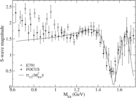
Figure 2: Magnitude of the $I_{K\pi}=1/2$ S-wave amplitude as a function of the $K\pi$ mass. Solid line: $|\tau_{\mbox{\tiny{1/2}}}\left(M^{2}_{K\pi}\right)|$ from Eq. (2) with arbitrary normalization. The data come from the phase-shift analysis of E791 (empty squares) Aitala12 ; Aitala3 and FOCUS collaboration (full inverted triangles) FOCUS1 ; FOCUS2 .

To be complete both isospin $1/2$ and $3/2$ are shown in Fig.  1 for comparison, and close to the minima of the magnitude of the $I_{K\pi}=1/2$ amplitude, the $3/2$ one becomes important, just anticipating what would come from the $D$ decay. The data for $I_{K\pi}=3/2$ is not shown as the effective range parametrization is the fit of the phase-shifts of this channel already presented in estabrooks .

III $D^{+}\to K^{-}\pi^{+}\pi^{+}$ decay with FSI

The collisions between the mesons in the final state of the $D^{+}\to K^{-}\pi^{+}\pi^{+}$ is represented diagrammatically in Fig. 3. The rescattering series is summed up in the $3\to 3$ transition matrix, which composes the full decay amplitude as (see MagPRD11 ):

$${\cal A}(k_{\pi},k_{\pi^{\prime}})=D(k_{\pi},k_{\pi^{\prime}})+\int\frac{d^{4}q_{\pi}d^{4}q_{\pi^{\prime}}}{(2\pi)^{8}}T(k_{\pi},k_{\pi^{\prime}};q_{\pi},q_{\pi^{\prime}})S_{\pi}(q_{\pi})\,S_{\pi}(q_{\pi^{\prime}})S_{K}(K-q_{\pi^{\prime}}-q_{\pi})D(q_{\pi},q_{\pi^{\prime}})\ ,$$ (8)

where the momentum of the pions are $k_{\pi}$ and $k_{\pi^{\prime}}$.

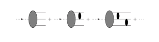
Figure 3: $D$ decay process into $K\pi\pi$ in the three-body ladder approximation. The source term (partonic amplitude) is represented by the gray blob. The fully off-shell $K\pi$ transition matrix is represented by the black blob.

The source of the mesons in the final state is given by the partonic amplitude expressed by the function $D(k_{\pi},k_{\pi^{\prime}})$, which is the first term of (8) and the gray blob in Fig. 3. It corresponds to a smooth amplitude given by the direct partonic decay amplitude determined by short-distance physics.

The second term of (8) brings the long range physics, which is represented by the sum of rescattering diagrams in the figure, has the $3\to 3$ transition matrix $T(k_{\pi},k_{\pi^{\prime}};q_{\pi},q_{\pi^{\prime}})$ convoluted with the source term, including the off-shell mesonic Feynman propagators $S_{i}(q_{i})=i(q_{i}^{2}-m_{i}^{2}+i\varepsilon)^{-1}$ , where the masses are $m_{i}$ $(i=\pi,K,\pi^{\prime})$ and the self-energies are disregarded. In the approximation considered in our work, the $3\to 3$ transition matrix sums the connected scattering series from ladder graphs. All possible $2\to 2$ collision terms are summed up in the $K\pi$ transition matrix, represented by the black blobs in Fig. 3. As a matter of fact, in the model we develop the T-matrix operator acts on the isospin space of the $K\pi\pi$ system, while ${D}(k_{\pi},k_{\pi^{\prime}})$ is an amplitude in the isospin space of the $K\pi\pi$ system.

III.1 Three-body Bethe-Salpeter approach

The final state interaction between the mesons in the three-body decay channel, are given by the full three-body T-matrix. It is a solution of the Bethe-Salpeter (BS) equation, which will be written in the Faddeev form. We consider spinless particles, disregard self-energies and three-body irreducible diagrams. Under these assumptions, the interactions between the mesons are assumed to be only due to two-body interactions. To be concise the momentum dependences will be omitted in the discussion below.

The three-particle BS equation for the T-matrix can be written as

$$T=\sum V_{i}+\sum V_{i}G_{0}\,T,$$ (9)

where the sum runs over the three two-body subsystems $i=(j,k)$. Formally, the potential in the four-dimensional equation is built by multiplying the two-body interaction $V^{(2)}_{jk}$ from all two-particle irreducible diagrams in which particles j and k interact, and by the inverse of the individual propagator of the spectator particle $i$, $S_{i}$

$$V=\sum_{i=1}^{3}V_{i}\ ;~{}~{}V_{i}=V_{(2)jk}S^{-1}_{i}~{}.$$ (10)

The propagator of particle $i$ is $S_{i}=\imath\left[k_{i}^{2}-m_{i}^{2}+\imath\epsilon\right]^{-1}$, $k_{i}$ being its four-momentum. The three-particle free Green’s function is

$$G_{0}=S_{i}S_{j}S_{k}\,.$$ (11)

Eq. (9) can now be rewritten in the Faddeev form. The transition matrix is decomposed as $T=T^{1}+T^{2}+T^{3}$ with the components $T^{i}=V_{i}+V_{i}\,G_{0}\,T$.

The relativistic generalization of the connected Faddeev equations is

$$T^{i}=T_{i}+T_{i}G_{0}\left(T^{j}+T^{k}\right),$$ (12)

where the two-body T-matrices are solutions of

$$T_{i}=V_{i}+V_{i}G_{0}T_{i},$$ (13)

within the three-body system. The full $3\to 3$ ladder scattering series is summed up by solving the integral equations for the Faddeev decomposition of the scattering matrix. Therefore, the three-body unitarity holds for the 3$\to$3 transition matrix built from the solution of the set of Faddeev equations (12) below the threshold of particle production from two-body collisions, where the two-body amplitude is unitary.

The full decay amplitude, Eq. (8), can be decomposed according to Eq. (12) as

$${\mathcal{A}}=D+\sum D^{i}\ ,$$ (14)

where the Faddeev components of the decay vertex are

$$D^{i}=T^{i}\,G_{0}\,D\ .$$ (15)

They are solutions of the connected equations

$$D^{i}=D_{i}+T_{i}G_{0}\left(D^{j}+D^{k}\right),$$ (16)

with

$$D_{i}=T_{i}\,G_{0}\,D.$$ (17)

The Faddeev equations for the decay vertex, Eqs. (16)-(17) are general once self-energies and three-body irreducible diagrams are disregarded. In the following they will be particularized to allow a separable form of the three-body decay amplitude.

III.2 s-channel two-meson amplitude

The matrix elements of the two-particle transition matrix is assumed to depend only on the Mandelstam s-variable and, within the three-body system, they read

$$T_{i}(k^{\prime}_{j},k^{\prime}_{k};k_{j},k_{k})=(2\pi)^{4}\tau_{i}(s_{i})\,S^{-1}_{i}(k_{i})\,\delta(k^{\prime}_{i}-k_{i})\ ,$$ (18)

where a delta of four-momentum conservation has been factorized out. The S-wave scattering amplitude $\tau_{i}(s_{i})$ of particles $i$ and $j$, depends on the Mandelstam variable $s_{i}=(k_{j}+k_{k})^{2}$. The three-body unitarity in our formulation is maintained, once the amplitude $\tau(s)$ is unitary.

Introducing Eq. (18) in Eqs. (16)-(17), one gets that

$$D^{i}(k_{j},k_{k})=\tau_{i}(s_{i})\xi^{i}(k_{i}),$$ (19)

where

$$\xi^{i}(k_{i})=\xi_{0}^{i}(k_{i})+\int\frac{d^{4}q_{j}d^{4}q_{k}}{(2\pi)^{4}}\delta(k_{i}-q_{i})S_{j}(q_{j})S_{k}(q_{k})\left(D^{j}(q_{k},q_{i})+D^{k}(q_{i},q_{j})\right)\,,$$ (20)

and

$$\xi_{0}^{i}(k_{i})=\int\frac{d^{4}q_{j}}{(2\pi)^{4}}S_{j}(q_{j})S_{k}(K-k_{i}-q_{j})\,D(q_{i},q_{j})\,,$$ (21)

with $q_{k}=K-k_{i}-q_{j}$. One can simplify the form of Eq. (20) by using the separation of the momentum dependences given by Eq. (19),

$$\xi^{i}(k_{i})=\xi_{0}^{i}(k_{i})+\int\frac{d^{4}q_{j}d^{4}q_{k}}{(2\pi)^{4}}\delta(k_{i}-q_{i})S_{j}(q_{j})S_{k}(q_{k})\left(\tau_{j}(s_{j})\xi^{j}(q_{j})+\tau_{k}(s_{k})\xi^{k}(q_{k})\right)\ ,$$ (22)

and, integrating the $\delta$’s, the formula is simplified to

$$\xi^{i}(k_{i})=\xi^{i}_{0}(k_{i})+\int\frac{d^{4}q_{j}}{(2\pi)^{4}}S_{j}(q_{j})S_{k}(K-k_{i}-q_{k})\tau_{j}(s_{j})\xi^{j}(q_{j})+\int\frac{d^{4}q_{k}}{(2\pi)^{4}}S_{j}(K-k_{i}-q_{k})S_{k}(q_{k})\tau_{k}(s_{k})\xi^{k}(q_{k})\ .$$ (23)

The separable form of the two-body T-matrix allows to simplify the integral equation for the Faddeev components of the vertex function, reducing it to a four-dimensional integral equation in one momentum variable.

The full decay amplitude considering the final state interaction computed with Eq. (19) reduces to the expression

$${\mathcal{A}}_{0}(k_{i},k_{j})=D(k_{i},k_{j})+\sum_{\alpha}\tau(s_{\alpha})\xi^{\alpha}(k_{\alpha})\ ,$$ (24)

where all the mesons in the three-body decay channel interact. The subindex in ${\cal A}_{0}$ just denotes the s-wave two-meson scattering.

The complex function $\xi(k_{i})$ in Eq. (24) carries the three-body rescattering effect by an amplitude and phase depending on the bachelor meson on-mass-shell momentum, while $\tau(s_{i})$ takes into account two-meson resonances. In the particular case of the $D^{+}\to K^{-}\pi^{+}\pi^{+}$ decay, and assuming that the identical pions do not interact, Eq. (8) reduces to Eq. (24) under the assumption that the matrix elements of the $K\pi$ transition matrix depend only on the Mandelstam s-variable.

III.3 $D^{+}\to K^{-}\pi^{+}\pi^{+}$ problem

The $K\pi\pi\to K\pi\pi$ rescattering process is accounted by the $D^{\pm}$ decay amplitude expressed by Eq. (24), where the bachelor amplitudes $\xi(k)$ are solutions of the connected Faddeev-like equations (23). Furthermore, we simplify the problem and disregard the interaction between the equal charged pions. The effective S-wave interaction between the kaon and pion is local on the fields with the $K\pi$ scattering amplitude $\tau_{i}(M^{2}_{K\pi})$ parameterized to reproduce the $K\pi$ S-wave phase-shift in the isospin $1/2$ and $3/2$ channels from the LASS experiment LASS , as presented in Sec. II.

The model assumptions for the $D^{+}\to K^{-}\pi^{+}\pi^{+}$ decay amplitude together with the chosen $K\pi$ S-wave amplitude, reduces Eq. (24) to

$${\mathcal{A}}_{0}(k_{\pi},k_{\pi^{\prime}})=D(k_{\pi},k_{\pi^{\prime}})+\tau(M^{2}_{K\pi})\xi(k_{\pi^{\prime}})+\tau(M^{2}_{K\pi^{\prime}})\xi(k_{\pi})\ ,$$ (25)

where the interaction between the identical pions is suppressed. The amplitude given in Eq. (25) is a sensible representation of the decay process, where the $K\pi$ resonant and nonresonant scattering phases are shifted by the momentum dependent bachelor phase from the three-body rescattering. The bachelor pion on-mass-shell momentum is given by

$$|{\mathbf{k}}_{\pi}|=\left[\left(\frac{M_{D}^{2}+m_{\pi}^{2}-M^{2}_{K\pi^{\prime}}}{2\,M_{D}}\right)^{2}-m_{\pi}^{2}\right]^{\frac{1}{2}}\ ,$$ (26)

with an analogous expression for $|{\mathbf{k}}_{\pi^{\prime}}|$. This implies that each rescattering term in Eq. (25) is a function only of $M^{2}_{K\pi}$ or $M^{2}_{K\pi^{\prime}}$.

The resummation of the three-body scattering series results in an inhomogeneous integral equation for the function $\xi(k)$ of the bachelor momentum,

$$\xi(k)=\xi_{0}(k)+\int\frac{d^{4}q}{(2\pi)^{4}}\tau\left((K-q)^{2}\right)\,S_{K}(K-k-q)\,S_{\pi}(q)\,\xi(q),$$ (27)

derived from Eq. (23) and shown diagrammatically in Fig. 4. Note that for convenience, the diagrammatic representation of the integral equation for the product $\tau\left(M^{2}_{K\pi^{\prime}}\right)\xi(k_{\pi})$ in presented in the figure.

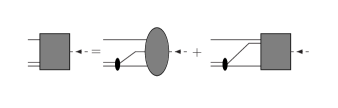
Figure 4: Diagrammatic representation of the integral equation for the three-body function $\tau(M^{2}_{K\pi^{\prime}})\xi(k_{\pi})$ (gray box). The driving term contains the partonic amplitude convoluted with the two-body scattering amplitude (black).

The driving term

$$\xi_{0}(k)=\int\frac{d^{4}q}{(2\pi)^{4}}S_{\pi}(q)S_{K}(K-k-q)D(k,q),$$ (28)

carries the partonic decay amplitude to the rescattering process. The second term in the rhs of Eq. (27) comes from three-body connected diagrams. For example, the lowest order rescattering term is the connected amplitude given by the third diagram in Fig. 3.

Physically, the three-body rescattering in Eq. (27) is built by mixing resonances of the two possible $K\pi$ pairs, and it is a function of the momentum of the bachelor pion. Therefore, we can say that the decay amplitude has two contributions: one that is a smooth function of the momentum of the pions, $D(k_{\pi},k_{\pi^{\prime}})$, and another one, $\tau\left(M^{2}_{K\pi^{\prime}}\right)\xi(k_{\pi})$, that contains the result of the three-body rescattering, which modulates the $K\pi$ scattering amplitude.

The $K\pi$ S-wave amplitude $\tau$ is an isospin conserving operator acting on the isospin states $1/2$ and $3/2$. The second and third terms in the rhs of Eq. (25) carry the full effect of the final state interaction through the $K\pi$ scattering amplitude, considered an operator in isospin space, $\tau$, times a spectator amplitude, $\xi$, that contains the three-body rescattering contributions. The solution of Eq. (27) built the rescattering series, and the term $\tau(M^{2}_{K\pi})\xi(k_{\pi^{\prime}})+\tau(M^{2}_{K\pi^{\prime}})\xi(k_{\pi})$ of the decay correspond to the sum of the second, third and higher order diagrams depicted in Fig. 3. They represent the full hadronic rescattering series of the $K\pi\pi$ system, disregarding three-body irreducible diagrams.

III.4 Phase and Amplitude Separation

The S-wave decay amplitude for the $D\to K^{-}\pi^{+}\pi^{+}$ from Eq. (25) can be written as a Bose-symmetrized complex function with respect to the identical pions,

$${\cal A}_{0}=A_{0}(M^{2}_{K\pi},M^{2}_{K\pi^{\prime}})+A_{0}(M^{2}_{K\pi^{\prime}},M^{2}_{K\pi}).$$ (29)

where $A_{0}$ are complex functions of the two invariant masses squared, $M^{2}_{K\pi}=(K-k_{\pi^{\prime}})^{2}$ and $M^{2}_{K\pi^{\prime}}=(K-k_{\pi})^{2}$, which specify the decay kinematics.

For the $D\to K^{-}\pi^{+}\pi^{+}$ S-wave amplitude in our model, the dependence on the $K\pi$ subsystem mass of $A_{0}(M^{2}_{K\pi^{\prime}},M^{2}_{K\pi})$ can be reduced to a complex function of only one variable $M^{2}_{K\pi^{\prime}}$ as

$$A_{0}(M^{2}_{K\pi^{\prime}})=a_{0}(M^{2}_{K\pi^{\prime}})e^{i\Phi_{0}(M^{2}_{K\pi^{\prime}})}=\frac{1}{2}\langle K\pi\pi|D\rangle+\langle K\pi\pi|\tau(M^{2}_{K\pi^{\prime}})|\xi(k_{\pi})\rangle,$$ (30)

where the bachelor pion on-mass-shell momentum is written as a function $M^{2}_{K\pi^{\prime}}$ as given by Eq. (26), and $|K\pi\pi\rangle$ represents the state in isospin space.

IV FSI Light-Front Dynamics in Heavy Meson Decay

The projection onto the light-front (LF) of the four-dimensional field-theoretical heavy meson three-particle decay amplitude with FSI, as expressed by Eq. (8), reduces it to a three-dimensional form. The coupled set of Eqs. (16) for the Faddeev components of the decay amplitude are turned into three-dimensional forms, simplifying the numerical treatment to solve them. We follow the LF projection technique of four-dimensional Bethe-Salpeter like equations as developed in Ref. sales00 based on the quasi-potential approach (QPA). The reduced amplitudes derived using the tools developed in a series of works sales00 ; MarPRD07 ; MarPoS08 ; MarFBS08 ; MarPRD08 and reviewed in FredFBS11 , depends only three-dimensional variables, namely, the kinematical LF momentum $\underline{k}\equiv(k^{+},\vec{k}_{\perp})$, defined by $k^{+}=k^{0}+k^{3}$ and $\vec{k}_{\perp}=\{k_{x},k_{y}\}$. The phase-space integration is normalized according to $dk^{+}d^{2}k_{\perp}/2(2\pi)^{3}$.

IV.1 QPA and Decay Amplitude

The potential in the four-dimensional equation for the three-boson BSE is given by Eq. (10) and in terms of the quasi-potential formulation, the BSE for the transition matrix Eq. (9), is substituted by

$$T=W+W\widetilde{G}_{0}T\ .$$ (31)

The quasi-potential $W$ and auxiliary Green’s function $(\widetilde{G}_{0})$ keep the dynamical content of the original BSE, when $W$ is the solution of

$$W=V+V\Delta_{0}W\ ,$$ (32)

with $\Delta_{0}:=G_{0}-\widetilde{G}_{0}$. The decay amplitude given by Eqs. (14) and (15), can be written in terms of the full three-body T-matrix as

$${\cal A}=D+T\,G_{0}\,D\ ,$$ (33)

and inserting the QP equation (31) in Eq. (33), one has that

$$T\,G_{0}\,D=W\,G_{0}\,D+W\,\widetilde{G}_{0}\,T\,G_{0}\,D\ .$$ (34)

The QPA allows to perform a three-dimensional reduction of the four-dimensional equation (33). In particular, the auxiliary Green’s function $\widetilde{G}_{0}$ can be conveniently chosen to project the four-dimensional three-body equation (34) onto the light-front hypersurface (see sales00 ), and formally it reads

$$\widetilde{G}_{0}:=G_{0}|~{}{g_{0}^{-1}}~{}|G_{0}\ ,$$ (35)

where $g_{0}=|G_{0}|$ is the free light-front resolvent, including phase-space factors. The “bar” operation on the right or on the left of a four-dimensional matrix element corresponds to the integration over $k^{-}=k^{0}+k^{3}$, which eliminates the relative light-front time between the particles. In our three-particle case, the elimination of the relative LF time requires an integration over two independent momenta $k^{-}$, due to four-momentum conservation, and we introduce the following operation

$$|A := \int dk_{1}^{-}dk_{2}^{-}\langle k_{1}^{-}k_{2}^{-}|A,$$

$$A| := \int dk_{1}^{-}dk_{2}^{-}A|k_{1}^{-}k_{2}^{-}\rangle,$$ (36)

with $A$ being a matrix element of an operator that has matrix elements function of two independent momenta after the center of mass motion is factorized.

Explicitly the free three-particle Green’s function is given by

$$\langle k_{1}^{-},k_{2}^{-}|G_{0}|k_{1}^{\prime-},k_{2}^{\prime-}\rangle=\frac{-i}{(2\pi)^{2}}\frac{\delta(k_{1}^{-}-k_{1}^{\prime-})}{\hat{k}_{1}^{+}\hat{k}_{2}^{+}(K^{+}-{\hat{k}_{1}}^{+}-\hat{k}_{2}^{+})(k_{1}^{-}-\hat{k}_{1on}^{-})}\\ \times\frac{\delta(k_{2}^{-}-k_{2}^{\prime-})}{(k_{2}^{-}-\hat{k}_{2on}^{-})(K^{-}-k_{1}^{-}-k_{2}^{-}-(K-\hat{k}_{1}-\hat{k}_{2})_{on}^{-})}~{},$$ (37)

where the hat means operator character and the on-minus-shell momentum $k^{-}_{ion}=(\vec{k}^{2}_{\perp}+m^{2}_{i})/k^{+}$. The on-minus-shell momentum $(K-\hat{k}_{1}-\hat{k}_{2})_{on}^{-}$ carries the mass of the third particle $m_{3}$. By performing the LF projection using Eq. (36), the free LF Green’s function comes as

$$g_{0}(\underline{k}_{1},\underline{k}_{2})=\frac{i\theta(K^{+}-k_{1}^{+}-k_{2}^{+})\theta(k_{1}^{+})\theta(k_{2}^{+})}{k_{1}^{+}k_{2}^{+}(K^{+}-{k_{1}}^{+}-k_{2}^{+})(K^{-}-k_{1on}^{-}-k_{2on}^{-}-(K-k_{1}-k_{2})_{on}^{-})}~{},$$ (38)

In Refs. sales00 ; FredFBS11 the reader can follow the details of the formal manipulations within QPA used to project onto the light-front the BSE. Two convenient operators were introduced in Ref. MarPRD08 , which helps to make the notation more transparent, namely the so-called free light-front reversed operators

$$\overline{\Pi}_{0}=G_{0}|~{}g_{0}^{-1}\,,\,\,\Pi_{0}=g_{0}^{-1}~{}|G_{0}\ ,$$ (39)

which can only be applied to the right and to left of a three-body four-dimensional quantity, respectively. These operators also transforms a tridimensional quantity to four dimensional ones, when acting on the left and on the right of an amplitude dependent on the kinematical light-front momenta, respectively. For example, with these operators, we have that the auxiliary Green’s function (35) is simply written as

$$\widetilde{G}_{0}=\overline{\Pi}_{0}\,g_{0}\,\Pi_{0}.$$ (40)

Our aim is to obtain the decay amplitude of the heavy meson in three mesons in the final state, using the three-dimensional projection onto the LF of Eq. (34). By applying the projection operator $\Pi_{0}$ in Eq. (34), we get that

$$\Pi_{0}T\,G_{0}\,D=\Pi_{0}W\,G_{0}\,D+\Pi_{0}W\,\widetilde{G}_{0}\,T\,G_{0}\,D\ ,$$ (41)

which translates to

$$D_{LF}\equiv|G_{0}TG_{0}D=|G_{0}WG_{0}D+w\,g_{0}D_{LF},$$ (42)

after the explicit form given in Eq. (39) is used. The function $D_{LF}$ depends only on the independent kinematical LF momenta of the particles, and the key dynamical ingredient is the effective LF potential $w=|G_{0}\,W\,G_{0}|$ containing the interaction among the three particles.

IV.2 Effective LF interaction for three-particles

In order to calculate $w$, we decompose the QP Eq. (32) in three terms, each given by

$$W_{i}=V_{i}+V_{i}\,\Delta_{0}\,W~{}$$ (43)

with $W$ being the sum over the Faddeev components, i.e., $W=\sum_{i}W_{i}$, and $w=\sum_{i}w_{i}=\sum_{i}|G_{0}\,W_{i}\,G_{0}|$.

The integral equation for the Faddeev component of the quasi-potential is obtained from the classical form by reintroducing $W$ as a sum of three terms in Eq. (43), giving

$$W_{i}=V_{i}+V_{i}\Delta_{0}(W_{i}+W_{j}+W_{k})\,$$ (44)

which can be rewritten as $(1-V_{i}\Delta_{0})W_{i}=V_{i}+V_{i}\Delta_{0}(W_{j}+W_{k})$, and multiplying to the right by $(1-V_{i}\Delta_{0})^{-1}$, one has that

$$W_{i}=W_{(2)i}+W_{(2)i}\Delta_{0}(W_{j}+W_{k}),$$ (45)

where the two-body quasi-potential within the three-body system is

$$W_{(2)i}=V_{i}+V_{i}\Delta_{0}W_{(2)i},$$ (46)

for particle $i$ acting as a spectator.

The solution of Eq. (45) is obtained in a form of an expansion in powers of $V_{i}$ where the series for the two-body quasi-potential, $W_{(2)i}=V_{i}+V_{i}\Delta_{0}V_{i}+V_{i}\Delta_{0}V_{i}\Delta_{0}V_{i}+\cdots$, is used, and terms in $V_{i}$ collected. The result is

$$W_{i}=V_{i}+V_{i}\Delta_{0}(V_{i}+V_{j}+V_{k})+V_{i}\Delta_{0}(V_{i}+V_{j}+V_{k})\Delta_{0}(V_{i}+V_{j}+V_{k})+\dots\,.$$ (47)

The leading order (LO) and next-to-leading-order (NLO) terms, the first and second power in the interaction $V_{i}$, are given by $W^{LO}_{i}=V_{i}$ and by $W^{NLO}_{i}=V_{i}+V_{i}\Delta_{0}(V_{i}+V_{j}+V_{k})$, respectively. Therefore, the Faddeev components of LF effective potential in LO and NLO are written in terms of the above expansion as

$$w^{LO}_{i} ={g_{0}^{-1}}~{}|G_{0}V_{i}G_{0}|~{}g_{0}^{-1}\ ,$$ (48)

$$w^{NLO}_{i} =w^{LO}_{i}+{g_{0}^{-1}}|G_{0}V_{i}\Delta_{0}(V_{i}+V_{j}+V_{k})G_{0}|~{}g_{0}^{-1}~{}.$$ (49)

The effective interactions $w_{i}$ builds the dynamical equation for the decay amplitude $D_{LF}$, Eq. (42), and the leading order calculation corresponds to a truncation at the valence states, which will be used in the next to built model for the heavy meson decay. We should note that the NLO interaction includes induced light-front three-body forces, namely terms like $g_{0}^{-1}|G_{0}\,V_{i}\Delta_{0}\,V_{j}\,G_{0}|~{}g_{0}^{-1}$, and already pointed out in KarFBS09 .

IV.3 LF Faddeev equations for $D_{LF}$

The LF projected decay amplitude solution of Eq. (42) is decomposed in a sum $D_{LF}=\sum_{i}D^{i}_{LF}$, where the Faddeev components are

$$D^{i}_{LF}=|G_{0}W_{i}G_{0}D+w_{i}\,g_{0}D_{LF}.$$ (50)

The standard manipulation leads to

$$D^{i}_{LF}=d^{i}_{LF,0}+t_{i}\,g_{0}\left(D^{j}_{LF}+D^{k}_{LF}\right),$$ (51)

where $d^{i}_{LF,0}=(1-w_{i}g_{0})^{-1}|G_{0}W_{i}G_{0}D$ and the reduced LF transition matrix $t_{i}$ is the solution of $t_{i}=w_{i}-w_{i}g_{0}t_{i}$. Assuming, that the partonic amplitude $D$ is weakly dependent in $k^{-}$ and the main dependence on $k^{-}$ in the integrand comes from the free propagator and $W_{i}$, we can write that

$$d^{i}_{LF,0}=(1-w_{i}g_{0})^{-1}|G_{0}W_{i}G_{0}|D=(1-w_{i}g_{0})^{-1}g_{0}w_{i}g_{0}D=t_{i}g_{0}D,$$ (52)

which will be exactly valid if $D$ is constant, as in our numerical application. The LF Faddev equation for the component of the vertex simply becomes

$$D^{i}_{LF}=t_{i}g_{0}D+t_{i}\,g_{0}\left(D^{j}_{LF}+D^{k}_{LF}\right),$$ (53)

and in next the model for $t_{i}$ is considered.

The LF front model for the two-body scattering amplitude comes from Eq. (18), using the relation $t_{i}=\overline{\Pi}_{0}T_{i}\Pi_{0}$:

$$\langle\underline{k}^{\prime}_{j},\underline{k}^{\prime}_{k}|g_{0}t_{i}g_{0}|\underline{k}_{j},\underline{k}_{k}\rangle=\langle\underline{k}^{\prime}_{j},\underline{k}^{\prime}_{k}|\,|G_{0}T_{i}G_{0}|\,|\underline{k}_{j},\underline{k}_{k}\rangle=\\ =(2\pi)^{4}\int dk_{j}^{\prime-}dk_{k}^{\prime-}\int dk_{j}^{-}dk_{k}^{-}\int dq_{j}^{-}dq_{k}^{-}\int dq_{j}^{\prime-}dq_{k}^{\prime-}\,S^{-1}_{i}(q_{i})\,\delta(q^{\prime}_{i}-q_{i})\langle k_{j}^{\prime-}k_{k}^{\prime-}|G_{0}|q_{j}^{\prime-}q_{k}^{\prime-}\rangle\,\\ \times\tau_{i}(s_{i})\,\langle q_{j}^{-}q_{k}^{-}|\ G_{0}|k_{j}^{-}k_{k}^{-}\rangle\\ =2\delta(\underline{K}-\underline{k}^{\prime}_{j}-\underline{k}^{\prime}_{k}-\underline{k}_{i})\int dk_{j}^{\prime-}dk_{j}^{-}dk_{i}^{-}i^{6}\,S_{j}(k^{\prime}_{j})S_{k}(K-k^{\prime}_{j}-k_{i})\\ \times\tau_{i}((K-k_{i})^{2})S_{i}(k_{i})S_{j}(k_{j})S_{k}(K-k_{j}-k_{i}).$$ (54)

Performing the Cauchy integration in each variable $k_{j}^{\prime-}$, $k_{j}^{-}$ and $k_{i}^{-}$, and given that $\tau_{i}((K-k_{i})^{2})$ is analytical in the lower-half of the $k^{-}_{i}$ complex-plane, the result is

$$\langle\underline{k}^{\prime}_{j},\underline{k}^{\prime}_{k}|t_{i}|\underline{k}_{j},\underline{k}_{k}\rangle=2(2\pi)^{3}k^{+}_{i}\delta(\underline{k}^{\prime}_{i}-\underline{k}_{i})\tau_{i}\left(M^{2}_{jk}\right)\ ,$$ (55)

where $M^{2}_{jk}=(K-k_{ion})^{2}$. Owing to the separable form of the two-body amplitude, the Faddeev component of the decay amplitude separates as

$$D^{i}_{LF}(\underline{k}_{j},\underline{k}_{k})=\tau_{i}\left(M_{jk}^{2}\right)\xi^{i}(\underline{k}_{i}),$$ (56)

as also happens for the four-dimensional case shown in Eq. (19).

The integral equation for the reduced decay amplitude, $\xi^{i}(\underline{k}_{i})$ becomes

$$\xi^{i}(\underline{k}_{i})=\xi^{i}_{0}(\underline{k}_{i})+\frac{i}{2(2\pi)^{3}}\int_{0}^{K^{+}-k^{+}_{i}}\frac{dq^{+}_{j}}{q^{+}_{j}(K^{+}-k^{+}_{i}-q^{+}_{j})}\int d^{2}q_{j\perp}\frac{\tau_{j}\left((K-q_{jon})^{2}\right)\xi^{j}(\underline{q}_{j})}{K^{-}-k^{-}_{ion}-q^{-}_{jon}-(K-k_{i}-q_{j})^{-}_{on}+i\varepsilon}\\ +\frac{i}{2(2\pi)^{3}}\int_{0}^{K^{+}-k^{+}_{i}}\frac{dq^{+}_{k}}{q^{+}_{k}(K^{+}-k^{+}_{i}-q^{+}_{k})}\int d^{2}q_{k\perp}\frac{\tau_{k}\left((K-q_{kon})^{2}\right)\xi^{k}(\underline{q}_{k})}{K^{-}-k^{-}_{ion}-(K-k_{i}-q_{k})^{-}_{on}-q^{-}_{kon}+i\varepsilon},$$ (57)

where

$$\xi^{i}_{0}(\underline{k}_{i})=\frac{i}{2(2\pi)^{3}}\int_{0}^{K^{+}-k^{+}_{i}}\frac{dq^{+}_{j}}{q^{+}_{j}(K^{+}-k^{+}_{i}-q^{+}_{j})}\int d^{2}q_{j\perp}\frac{D(\underline{q}_{j};\underline{k}_{i})}{K^{-}-k^{-}_{ion}-q^{-}_{jon}-(K-k_{i}-q_{j})^{-}_{on}+i\varepsilon}.$$ (58)

Rewriting Eqs. (57) and (58) in terms of momentum fractions, one gets

$$\xi^{i}(y,\vec{k}_{\perp})=\xi^{i}_{0}(y,\vec{k}_{\perp})+\frac{i}{2(2\pi)^{3}}\int_{0}^{1-y}\frac{dx}{x(1-x-y)}\int d^{2}q_{\perp}\left[\frac{\tau_{j}\left(M^{2}_{ik}(x,q_{\perp})\right)\xi^{j}(x,\vec{q}_{\perp})}{M^{2}-M_{0}^{2}(x,\vec{q}_{\perp};y,\vec{k}_{\perp})+i\varepsilon}+(j\leftrightarrow k)\right],$$ (59)

where $M^{2}=K^{\mu}K_{\mu}$, $y=k^{+}_{i}/K^{+}$, $x=q^{+}_{j}/K^{+}$ or $x=q^{+}_{k}/K^{+}$ in the first or second integral in the right-hand side of the equation. The free three-body squared mass is

$$M_{0}^{2}(x,\vec{q}_{\perp};y,\vec{k}_{\perp})=\frac{k_{\perp}^{2}+m^{2}_{i}}{y}+\frac{q_{\perp}^{2}+m^{2}_{j}}{x}+\frac{(\vec{k}_{\perp}+\vec{q}_{\perp})^{2}+m^{2}_{k}}{1-x-y}.$$ (60)

The argument of the two-body amplitude $\tau_{j}\left(M^{2}_{ik}(x,q_{\perp})\right)$ should be understood as

$$M_{ik}^{2}(x,q_{\bot})=(1-x)\left(M^{2}-\frac{q_{\bot}^{2}+m_{j}^{2}}{x}\right)-q_{\bot}^{2}\ .$$ (61)

The driven term in Eq. (59) is rewritten as

$$\xi^{i}_{0}(y,\vec{k}_{\perp})=\frac{i}{2(2\pi)^{3}}\int_{0}^{1-y}\frac{dx}{x(1-y-x)}\int d^{2}q_{\perp}\frac{D(x,\vec{q}_{\perp};y,\vec{k}_{\perp})}{M^{2}-M_{0}^{2}(x,\vec{q}_{\perp};y,\vec{k}_{\perp})+i\varepsilon}.$$ (62)

The LF model for the three-body heavy meson decay modeled by Eqs. (56) and (59) assumes the dominance of the valence state in the intermediate state propagations and the $s$-channel description of the two-meson amplitude. To be complete, the LF counterpart of the decay amplitude in Eq. (24) is

$${\mathcal{A}}_{0}=D+\sum_{\alpha}\tau(s_{\alpha})\xi^{\alpha}(y,\vec{k}_{\perp})\ ,$$ (63)

where $s_{\alpha}=(K-k_{\alpha on})^{2}$ and the partonic function $D$ is a function on the momentum of the on-mass-shell particles in the decay channel. We concluded the general formalism for the calculation of the heavy meson decay amplitude in three spinless mesons. For the $D^{+}\to K^{-}\pi^{+}\pi^{+}$ process Eq. (63) reduces to

$${\mathcal{A}}_{0}(k_{\pi},k_{\pi^{\prime}})=D(k_{\pi},k_{\pi^{\prime}})+\tau(M^{2}_{K\pi})\xi(\underline{k}_{\pi^{\prime}})+\tau(M^{2}_{K\pi^{\prime}})\xi(\underline{k}_{\pi})\,,$$ (64)

where as we have assumed, also in the four-dimensional case, see Eq. (25), the interaction between the identical pions is suppressed. In order to keep the rotation invariance of the calculation, the $z-$direction is chosen transverse to the decay plane in the rest frame of the $D^{\pm}$ meson. This choice makes optimal use of the kinematical nature of the rotation in the transverse plane, adopted as the plane where the momentum of each meson in the final state are.

V LF model for $D^{+}\to K^{-}\pi^{+}\pi^{+}$ decay

The light-front model for the $D^{+}\to K^{-}\pi^{+}\pi^{+}$ decay with FSI is given by the inhomogeneous integral equation for the bachelor meson amplitude (59), with the driven term (62), and full decay amplitude written in Eq. (64). Besides the partonic amplitude, which defines the driven term for the bachelor amplitude, the two-meson scattering amplitude is the input for the calculations. We disregard the $\pi\pi$ interaction in isospin $1$ charged states, and consider only the neutral channels $K\pi$ states. The isospin states for $K^{\mp}\pi^{\pm}$ are $I_{K\pi}=1/2$ and $I_{K\pi}=3/2$, the parametrization of the S-waves amplitudes given in Sec. II. The dominant $K\pi$ amplitude is the resonant $I_{K\pi}=1/2$ one below $K^{*}_{0}(1430)$, but above it the $I_{K\pi}=3/2$ amplitude has a comparable contribution for the scattering LASS . Therefore, to explore the available phase-space for the $D$ decay above $K^{*}_{0}(1430)$, one has to consider not only $I_{K\pi}=1/2$ but also $I_{K\pi}=3/2$. Indeed, below $K^{*}_{0}(1430)$ the calculations were previously performed in Ref. MagPRD11 . It was also included the $I_{K\pi}=3/2$ interaction in the $D$ decay amplitude up to two-loops in Ref. MagPoS12 .

In this section, we present a isospin conserving light-front model, including interaction in both $K\pi$ isospin states, and perform calculations up to three-loops, in order to check the convergence of the results. The possible total isospin states $(I_{T})$ are $5/2$ and $3/2$ with $I_{T}^{z}=\pm 3/2$. The bachelor amplitude, solution of Eq. (59), carries the total isospin index, and the interacting pair isospin, namely $\xi^{I_{T}^{z}}_{I_{T},I_{K\pi}}(y,k_{\bot})$, we keep for convenience, the isospin projection. We restrict our calculations only to s-wave states and the bachelor amplitude depends only on $|\vec{k}_{\perp}|\equiv k_{\perp}$. The partonic decay amplitude has now to be projected on two $K\pi$ isospin states, and total isospin, i.e.,

$$\left|D\right>=\sum_{I_{T},I_{K\pi}}\alpha^{I_{T}^{z}}_{I_{T},I_{K\pi}}\left|I_{T},I_{K\pi},I_{T}^{z}\right>+\sum_{I_{T},I_{K\pi^{\prime}}}\alpha^{I_{T}^{z}}_{I_{T},I_{K\pi^{\prime}}}\left|I_{T},I_{K\pi^{\prime}},I_{T}^{z}\right>.$$ (65)

The projected LF inhomogeneous integral equations for the bachelor amplitudes $\xi^{I_{T}^{z}}_{I_{T},I_{K\pi}}$ built from Eq. (59), are given by a set of isospin coupled systems, with the driven term weighted by the partonic amplitude (65), and written as

$$\xi^{I_{T}^{z}}_{I_{T},I_{K\pi}}(y,k_{\bot})=\left<I_{T},I_{K\pi},I_{T}^{z}|D\right>\xi_{0}(y,k_{\bot})+\frac{i}{2}\sum_{I_{K\pi^{\prime}}}R^{I_{T}^{z}}_{I_{T},I_{K\pi},I_{K\pi^{\prime}}}\int_{0}^{1-y}\frac{dx}{x(1-y-x)}\int_{0}^{\infty}\frac{dq_{\bot}}{(2\pi)^{3}}\\ \times K_{I_{K\pi^{\prime}}}(y,k_{\bot};x,q_{\bot})\,\xi^{I_{T}^{z}}_{I_{T},I_{K\pi^{\prime}}}(x,q_{\bot}),$$ (66)

where the kernel carrying the isospin of the interacting pair is

$$K_{I_{K\pi^{\prime}}}(y,k_{\bot};x,q_{\bot})=\int_{0}^{2\pi}d\theta\,\,{q_{\bot}\,\tau_{I_{K\pi^{\prime}}}\left(M_{K\pi^{\prime}}^{2}(x,q_{\bot})\right)\over M_{D}^{2}-M_{0,K\pi\pi}^{2}(x,q_{\bot},y,k_{\bot})+i\varepsilon}.$$ (67)

The isospin recoupling coefficients in Eq. (66) are $R^{I_{T}^{z}}_{I_{T},I_{K\pi},I_{K\pi^{\prime}}}=\left<I_{T},I_{K\pi},I_{T}^{z}|I_{T},I_{K\pi^{\prime}},I_{T}^{z}\right>$. The free squared mass of the $K\pi\pi$ system is

$$M_{0,K\pi\pi}^{2}(x,q_{\bot},y,k_{\bot})=\frac{k_{\bot}^{2}+m_{\pi}^{2}}{y}+\frac{q_{\bot}^{2}+m_{\pi}^{2}}{x}+\frac{q_{\bot}^{2}+k_{\bot}^{2}+2q_{\bot}k_{\bot}\cos\theta+m_{K}^{2}}{1-x-y},$$ (68)

and the squared-mass of the virtual $K\pi$ system is

$$M_{K\pi}^{2}(z,p_{\bot})=(1-z)\left(M_{D}^{2}-\frac{p_{\bot}^{2}+m_{\pi}^{2}}{z}\right)-p_{\bot}^{2}.\,\,\,$$ (69)

The driving term is regularized by one subtraction, at the scale $\mu$, and one finite subtraction constant $\lambda(\mu^{2})$, and is written as

$$\xi_{0}(y,k_{\bot})=\lambda(\mu^{2})+\frac{i}{2}\int_{0}^{1}\frac{dx}{x(1-x)}\int_{0}^{2\pi}d\theta\int_{0}^{\infty}\frac{dq_{\bot}q_{\bot}}{(2\pi)^{3}}\left[\frac{1}{M_{K\pi}^{2}(y,k_{\bot})-M_{0,K\pi}^{2}(x,q_{\bot})+i\varepsilon}-\frac{1}{\mu^{2}-M_{0,K\pi}^{2}(x,q_{\bot})}\right],$$ (70)

where the free squared-mass of the virtual $K\pi$ system in the driven term is

$$M_{0,K\pi}^{2}(x,q_{\bot})=\frac{q_{\bot}^{2}+m_{\pi}^{2}}{x}+\frac{q_{\bot}^{2}+m_{K}^{2}}{1-x}.$$ (71)

Performing the angular and radial integrations one gets that

$$\xi_{0}(y,k_{\bot})=\lambda(\mu^{2})+\frac{i}{4}\int_{0}^{1}\frac{dx}{(2\pi)^{2}}\ln\frac{\Lambda_{1}}{\Lambda_{2}},$$ (72)

where

$$\Lambda_{1} =(1-x)(xM_{K\pi}^{2}(y,k_{\bot})-m_{\pi}^{2}+ix\varepsilon)-xm_{K}^{2}\ ,$$ (73)

$$\Lambda_{2} =(1-x)(x\mu^{2}-m_{\pi}^{2})-xm_{K}^{2}\ .$$ (74)

The light-front $D$ decay model with isospin dependence on the $K\pi$ pair will be explored further in two situations: $i)$ only $K\pi$ s-wave interaction in the resonant $I=1/2$ state (single-channel model); and $ii)$ $K\pi$ s-wave interaction in $I=1/2$ and 3/2 (coupled-channel model). In both cases we disregard the pion-pion interaction in $I=2$ states.

V.1 Phase and Amplitude Separation

The full $D\to K^{-}\pi^{+}\pi^{+}$ S-wave decay amplitude from the solution of Eq. (25) is symmetrized in respect to the identical pions as given in Eq. (29), and written as

$${\cal A}_{0}=A_{0}(M^{2}_{K\pi^{\prime}})+A_{0}(M^{2}_{K\pi}).$$ (75)

as each amplitude depends only on the Mandelstam s-variable of each $K\pi$ subsystem. In detail, each amplitude in Eq. (75) has the bachelor amplitude and $K\pi$ scattering amplitude, i.e.,

$$A_{0}(M^{2}_{K\pi^{\prime}}) = \sum_{I_{T},I_{K\pi^{\prime}},I_{T}^{z}}\left<K^{-}\pi^{+}\pi^{+}\right|\left.I_{T},I_{K\pi^{\prime}},I_{T}^{z}\right>\left[\frac{1}{2}\left<I_{T},I_{K\pi^{\prime}},I_{T}^{z}\right|\left.D\right>+\tau_{I_{K\pi}}(M^{2}_{K\pi^{\prime}})\xi^{I_{T}^{z}}_{I_{T},I_{K\pi^{\prime}}}(k_{\pi})\right]$$ (76)

$$= a_{0}(M^{2}_{K\pi^{\prime}})e^{i\Phi_{0}(M^{2}_{K\pi^{\prime}})}\ ,$$

where the projection onto the final $K\pi\pi$ isospin state is performed. In the bachelor amplitude the pion momentum is on-mass-shell and, due to the total momentum conservation, its modulus is defined by Eq. (26) as a function of $M^{2}_{K\pi^{\prime}}$.

VI Perturbative solutions

The perturbative solution of the integral equations for the bachelor amplitudes (66) in the different isospin channels, is found by iteration starting from the driving term. The terms in the perturbative series are obtained by loop integrations. The bachelor amplitude found from the driving term corresponds to a one-loop calculation. In Ref. MagPRD11 , a calculation up to two-loops were performed. For the single-channel model, we calculate up to three-loops to check the convergence of the perturbative series. For the coupled-channel, where the total isospin states $I=3/2$ can be formed either by coupling $I_{K\pi}=1/2$ or $I_{K\pi}=3/2$, we also perform calculations up to three-loops. Also the $I_{T}=5/2$ is considered, where the only contribution from the $K\pi$ interaction happens in the isospin 3/2 states. Indeed such contributions to the $K\pi\pi$ phase are marginal.

VI.1 Interaction in $I_{K\pi}=1/2$ state

Our aim in the single channel example is to solve numerically the light-front Eq. (66) for the bachelor amplitude when we consider only $K\pi$ interaction in the resonant isospin 1/2 states. In this case, Eq. (66) reduces to

$$\xi^{\mbox{\tiny{3/2}}}_{\mbox{\tiny{3/2,1/2}}}(y,k_{\bot})=\frac{1}{6}\sqrt{\frac{2}{3}}\xi_{0}(y,k_{\bot})-\frac{i}{3}\int_{0}^{1-y}\frac{dx}{x(1-y-x)}\int_{0}^{\infty}\frac{dq_{\bot}}{(2\pi)^{3}}K_{\mbox{ \tiny{1/2}}}(y,k_{\bot};x,q_{\bot})\,\xi^{\mbox{ \tiny{3/2}}}_{\mbox{\tiny{3/2,1/2}}}(x,q_{\bot}),$$ (77)

where the driving term is computed by considering only $\alpha^{3/2}_{3/2,1/2}$ in Eq. (65) nonvanishing and equal to unity, and the partonic decay amplitude is assumed momentum independent.

The perturbative solution of the integral equation (77) up to three-loops is given by

$$\xi^{\mbox{\tiny{3/2}}}_{\mbox{\tiny{3/2,1/2}}}(y,k_{\bot})=\frac{1}{6}\sqrt{\frac{2}{3}}\xi_{0}(y,k_{\bot})-\frac{i}{3}\left(\frac{1}{6}\sqrt{\frac{2}{3}}\right)\int_{0}^{\infty}\frac{dq_{\bot}}{(2\pi)^{3}}\int_{0}^{1-y}dx\,K_{\mbox{\tiny 1/2}}(y,k_{\bot};x,q_{\bot})\,\xi_{0}(x,q_{\bot})+\\ -\frac{1}{9}\left(\frac{1}{6}\sqrt{\frac{2}{3}}\right)\int_{0}^{\infty}\frac{dq_{\bot}}{(2\pi)^{3}}\int_{0}^{1-y}dx\,K_{\mbox{\tiny 1/2}}(y,k_{\bot};x,q_{\bot})\int_{0}^{\infty}\frac{dq_{\bot}^{\prime}}{(2\pi)^{3}}\int_{0}^{1-x}dx^{\prime}\,K_{\mbox{\tiny 1/2}}(x,q_{\bot};x^{\prime},q_{\bot}^{\prime})\,\xi_{0}(x^{\prime},q_{\bot}^{\prime})+\cdots$$ (78)

where $K_{\mbox{\tiny 1/2}}(x,q_{\bot},y,k_{\bot})$ is defined by Eq. (67).

For the numerical calculation of the bachelor amplitude up to three-loops in Eq. (78), we introduce a momentum cut-off, $\Lambda=2$ GeV for numerical convenience. Note that the imaginary part of the s-wave $K\pi$ amplitude from Eqs. (2) and (3) in the unphysical region, as plotted in Fig. 5, goes fast enough to zero for large momentum and shows that the momentum loop integrals in the perturbative calculation in Eq. (78) are finite. In the figure, we plot the real and imaginary parts of the $K\pi$ amplitude as a function of $z$ and $p_{\bot}$, which are the arguments of the squared mass of the interacting virtual $K\pi$ system given in Eq. (69), and corresponds to $x$ and $q_{\bot}$ in the kernel of Eq. (78), respectively.

Figure 5: Real and imaginary parts of the $I=1/2$ S-wave $K\pi$ amplitude as a function of $p_{\bot}$ for some $z$ values in the unphysical mass region. The $M^{2}_{K\pi}$ value is related to $p_{\bot}$ and $z$ through Eq. (69).

The analytic continuation of the s-wave isospin $1/2$ $K\pi$ scattering amplitude to the unphysical region of the $K\pi$ amplitude, i.e., for $M^{2}_{K\pi}<(m_{K}+m_{\pi})^{2}$, is chosen as the imaginary part of $\tau_{1/2}$, with the effective range in Eq. (5) turned off. For the isospin $3/2$ case, also the effective range in Eq. (6) is disregarded in the unphysical region in order to avoid bound states poles in the S-matrix. Note that in the kernel of the integral equations only the imaginary part of the $K\pi$ amplitude is used in the unphysical region, which corresponds to a real scattering amplitude, as it should be.

In our calculations of Eq. (78), we have considered finite values of for $\varepsilon$ in the meson propagators, we use 0.2 and 0.3 GeV, which induces absorption and mimics coupling to other decay channels. The subtraction constant in the driving term is chosen for $\mu^{2}=0$ to be $\lambda(0)=0.12+i0.06$, which matches the driving term computed in Ref. MagPRD11 . We test the change in the subtraction parameter, by keeping $\lambda(\mu^{2})$ fixed to $\lambda(0)$, while moving $\mu^{2}$.

In Fig. 6, we study the convergence of the loop expansion for the phase and amplitude of the bachelor function up to three-loops. We choose $\mu^{2}=(0.4,-0.1,-1)$ GeV² with $\varepsilon=0.3$ GeV². The values of $|\mu|$ are chosen within the hadronic scale between $\sim$ 0.3 to 1 GeV, spanning values of $\mu^{2}$ above and below zero in order to verify the sensitivity of the bachelor function. Irrespectively to the value of $\mu^{2}$, the 2-loops solution is good enough and can be used to compute the bachelor amplitude. However, the phase can be either positive or negative, but it increases with $M^{2}_{K\pi}$. For $\mu^{2}=-0.4$ GeV² and $\mu^{2}=-1$  GeV², the phase difference between the threshold and the maximum for the mass of the $K\pi$ system, the phase shows a quite large variation of about $60^{o}$. The modulus increases with $M^{2}_{K\pi}$ for all $\mu^{2}$ values.

Figure 6: Modulus and phase of $\xi^{\mbox{\tiny{3/2}}}_{\mbox{\tiny{3/2,1/2}}}$ for $\varepsilon=0.3$ GeV² and different $\mu^{2}$ values.

VI.2 Interaction in $I_{K\pi}=1/2$ and 3/2 states

The inclusion of the two possible isospin channels for the $K\pi$ interacting system, namely, $1/2$ and $3/2$, results in a coupled set of inhomogeneous integral equations from Eq. (66) for $I_{T}=3/2$, which reads

$$\xi^{\mbox{\tiny{3/2}}}_{\mbox{\tiny{3/2,1/2}}}(y,k_{\bot})=A_{w}\,\xi_{0}(y,k_{\bot})+\frac{iR^{\mbox{\tiny{3/2}}}_{\mbox{\tiny{3/2,1/2,1/2}}}}{2}\int_{0}^{1-y}\frac{dx}{x(1-y-x)}\int_{0}^{\infty}\frac{dq_{\bot}}{(2\pi)^{3}}K_{\mbox{\tiny 1/2}}(y,k_{\bot};x,q_{\bot})\,\xi^{\mbox{\tiny{3/2}}}_{\mbox{\tiny{3/2,1/2}}}(x,q_{\bot})+\\ +\frac{iR^{\mbox{\tiny{3/2}}}_{\mbox{\tiny{3/2,1/2,3/2}}}}{2(2\pi)^{3}}\int_{0}^{1-y}\frac{dx}{x(1-y-x)}\int_{0}^{\infty}\frac{dq_{\bot}}{(2\pi)^{3}}\,K_{\mbox{\tiny 3/2}}(y,k_{\bot};x,q_{\bot})\,\xi^{\mbox{\tiny{3/2}}}_{\mbox{\tiny{3/2,3/2}}}(x,q_{\bot}),$$ (79)

$$\xi^{\mbox{\tiny{3/2}}}_{\mbox{\tiny{3/2,3/2}}}(y,k_{\bot})=B_{w}\,\xi_{0}(y,k_{\bot})+\frac{iR^{\mbox{\tiny{3/2}}}_{\mbox{\tiny{3/2,3/2,1/2}}}}{2}\int_{0}^{1-y}\frac{dx}{x(1-y-x)}\int_{0}^{\infty}\frac{dq_{\bot}}{(2\pi)^{3}}\,K_{\mbox{\tiny 1/2}}(y,k_{\bot};x,q_{\bot})\,\xi^{\mbox{\tiny{3/2}}}_{\mbox{\tiny{3/2,1/2}}}(x,q_{\bot})+\\ +\frac{iR^{\mbox{\tiny{3/2}}}_{\mbox{\tiny{3/2,3/2,3/2}}}}{2}\int_{0}^{1-y}\frac{dx}{x(1-y-x)}\int_{0}^{\infty}\frac{dq_{\bot}}{(2\pi)^{3}}\,K_{\mbox{\tiny 3/2}}(y,k_{\bot};x,q_{\bot})\,\xi^{\mbox{\tiny{3/2}}}_{\mbox{\tiny{3/2,3/2}}}(x,q_{\bot}).$$ (80)

For $I_{T}=5/2$ Eq. (66) is single channel and interaction only in $I_{K\pi}=$3/2 is possible. In this case, the inhomogeneous equation for the bachelor amplitude is

$$\xi^{\mbox{\tiny{3/2}}}_{\mbox{\tiny{5/2,3/2}}}(y,k_{\bot})=C_{w}\,\xi_{0}(y,k_{\bot})+\frac{iR^{\mbox{\tiny{3/2}}}_{\mbox{\tiny{5/2,3/2,3/2}}}}{2}\int_{0}^{1-y}\frac{dx}{x(1-y-x)}\int_{0}^{\infty}\frac{dq_{\bot}}{(2\pi)^{3}}\,K_{\mbox{\tiny 3/2}}(y,k_{\bot};x,q_{\bot})\,\xi^{\mbox{\tiny{3/2}}}_{\mbox{\tiny{5/2,3/2}}}(x,q_{\bot}),$$ (81)

where the weights $A_{w}$, $B_{w}$ and $C_{w}$ appearing in the driving terms are computed from the initial distribution of isospin states from the partonic amplitude (65).

The weights in the driven terms of Eqs. (80) and (81) are computed from the overlap of isospin state with the initial isospin distribution of the decay from the partonic amplitude,

$$A_{w}=\frac{1}{2}\left<I_{T}=3/2,I_{K\pi}=1/2,I_{T}^{z}=3/2\right|\left.D\right>,\qquad$$ (82)

$$B_{w}=\frac{1}{2}\left<I_{T}=3/2,I_{K\pi}=3/2,I_{T}^{z}=3/2\right|\left.D\right>,\qquad$$ (83)

$$C_{w}=\frac{1}{2}\left<I_{T}=5/2,I_{K\pi}=3/2,I_{T}^{z}=3/2\right|\left.D\right>,\qquad$$ (84)

and, evaluating in details the isospin coefficients, one gets

$$A_{w} = \alpha^{\mbox{\tiny{3/2}}}_{\mbox{\tiny{3/2,1/2}}}(1+R^{\mbox{\tiny{3/2}}}_{\mbox{\tiny{3/2,1/2,1/2}}})+\alpha^{\mbox{\tiny{3/2}}}_{\mbox{\tiny{3/2,3/2}}}R^{\mbox{\tiny{3/2}}}_{\mbox{\tiny{3/2,1/2,3/2}}},\qquad$$ (85)

$$B_{w} = \alpha^{\mbox{\tiny{3/2}}}_{\mbox{\tiny{3/2,3/2}}}(1+R^{\mbox{\tiny{3/2}}}_{\mbox{\tiny{3/2,3/2,3/2}}})+\alpha^{\mbox{\tiny{3/2}}}_{\mbox{\tiny{3/2,1/2}}}R^{\mbox{\tiny{3/2}}}_{\mbox{\tiny{3/2,3/2,1/2}}},\qquad$$ (86)

$$C_{w} = \alpha^{\mbox{\tiny{3/2}}}_{\mbox{\tiny{5/2,3/2}}}(1+R^{\mbox{\tiny{3/2}}}_{\mbox{\tiny{5/2,3/2,3/2}}}).$$ (87)

The coefficients $\alpha$ appearing above comes from the initial decay amplitude (65), and now we define them in terms of the parameters $W_{i}$ ($i=1,2,3$), such that

$$\alpha^{\mbox{\tiny{3/2}}}_{\mbox{\tiny{3/2,1/2}}} = \frac{W_{1}}{2}\,C^{\mbox{\tiny{1/2 1 3/2}}}_{\mbox{\tiny{1/2 1 3/2}}}\,C^{\mbox{\tiny{1 1/2 1/2}}}_{\mbox{\tiny{1 -1/2 1/2}}}\,,$$ (88)

$$\alpha^{\mbox{\tiny{3/2}}}_{\mbox{\tiny{3/2,3/2}}} = \frac{W_{2}}{2}\,C^{\mbox{\tiny{3/2 1 3/2}}}_{\mbox{\tiny{1/2 1 3/2}}}\,C^{\mbox{\tiny{1 1/2 3/2}}}_{\mbox{\tiny{1 -1/2 1/2}}}\,,$$ (89)

$$\alpha^{\mbox{\tiny{3/2}}}_{\mbox{\tiny{5/2,3/2}}} = \frac{W_{3}}{2}\,C^{\mbox{\tiny{3/2 1 5/2}}}_{\mbox{\tiny{1/2 1 3/2}}}\,C^{\mbox{\tiny{1 1/2 3/2}}}_{\mbox{\tiny{1 -1/2 1/2}}}\,,$$ (90)

which in the particular case of $\left|D\right>=\left|K^{-}\pi^{+}\pi^{+}\right>$ one has that $W_{1}=W_{2}=W_{3}=1$.

To be complete, the respective Clebsch-Gordan and recoupling coefficients necessary for all computations are $\,C^{\mbox{\tiny{1/2 1 3/2}}}_{\mbox{\tiny{1/2 1 3/2}}}=1\,$, $\,C^{\mbox{\tiny{1 1/2 1/2}}}_{\mbox{\tiny{1 -1/2 1/2}}}=\sqrt{2/3}\,$, $\,C^{\mbox{\tiny{3/2 1 3/2}}}_{\mbox{\tiny{1/2 1 3/2}}}=-\sqrt{2/5}\,$, $\,C^{\mbox{\tiny{1 1/2 3/2}}}_{\mbox{\tiny{1 -1/2 1/2}}}=1/\sqrt{3}\,$, $\,C^{\mbox{\tiny{3/2 1 5/2}}}_{\mbox{\tiny{1/2 1 3/2}}}=\sqrt{3/5}\,$, $\,R^{\mbox{\tiny{3/2}}}_{\mbox{\tiny{3/2,1/2,1/2}}}=-2/3\,$, $\,R^{\mbox{\tiny{3/2}}}_{\mbox{\tiny{3/2,1/2,3/2}}}=\sqrt{5}/3\,$, $\,R^{\mbox{\tiny{3/2}}}_{\mbox{\tiny{3/2,3/2,3/2}}}=2/3\,$, $\,R^{\mbox{\tiny{3/2}}}_{\mbox{\tiny{3/2,3/2,1/2}}}=\sqrt{5}/3\,$, and $\,R^{\mbox{\tiny{3/2}}}_{\mbox{\tiny{5/2,3/2,3/2}}}=1\,$.

In terms of $W_{1}$, $W_{2}$, and $W_{3}$, the constants $A_{w}$, $B_{w}$, and $C_{w}$ are written as

$$A_{w} = \sqrt{\frac{1}{54}}(W_{1}-W_{2}),$$ (91)

$$B_{w} = \sqrt{\frac{5}{54}}(W_{1}-W_{2}),$$ (92)

$$C_{w} = \frac{W_{3}}{\sqrt{5}},$$ (93)

which implies that if $A_{w}=B_{w}$ only total isospin $5/2$ contributes to the decay. This happens, in particular, for the initial state of $\left|D\right>=\left|K^{-}\pi^{+}\pi^{+}\right>$. Therefore, the initial state should have be a mixture of states. Indeed, the fittings we will show suggest $W_{1}\neq W_{2}$ and $W_{3}$ smaller than $W_{1}$ or $W_{2}$.

Figure 7: Modulus and phase of $\xi^{I_{T}^{z}}_{I_{T},I_{K\pi}}$ for $\varepsilon=0.3$ GeV² and $\mu^{2}=-0.1$ GeV². The parameters in the the expansion of the initial state are $W_{1}=1$, $W_{2}=2$ and $W_{3}=0.2$.

We compute up to three-loops the bachelor amplitude from the coupled equations for $I_{T}=3/2$, Eq. (79), and for the single channel equation for $I_{T}=5/2$, Eq. (81), with momentum cut-off of $2$ GeV. In Fig. 7, we show results for $\varepsilon=0.3$ GeV² and $\mu^{2}=-0.1$ GeV², with $W_{1}=1$, $W_{2}=2$ and $W_{3}=0.2$. The convergence $\xi^{I_{T}^{z}}_{I_{T},I_{K\pi}}$ regarding the loop expansion is evident, and two-loop calculations are enough for our purposes. The bachelor amplitudes, present a considerable change in the phase and modulus, both increasing with $M_{K\pi}$.

VII Results for the Phase and Amplitude in the $D^{+}\to K^{-}\pi^{+}\pi^{+}$ decay

We will restrict our calculations up to two-loops as it was already shown in Sec. VI to be enough to compute bachelor amplitudes. Results for two cases will be given, for the single channel model with interaction restricted to $I_{K\pi}=1/2$, and the case where $I_{K\pi}=$ 1/2 and 3/2 interactions are present in the $K\pi\pi$ system.

VII.1 Single-channel with $I_{K\pi}=1/2$ interaction

The physical amplitude for the s-wave $D^{+}\to K^{-}\pi^{+}\pi^{+}$ decay is obtained by considering only $K\pi$ scattering in isospin $1/2$ states, with the bachelor amplitude calculated by collecting the appropriate contributions up to two-loops in Eq. (78). It is parametrized according to Eq. (76) and written as

$$A_{0}(M^{2}_{K\pi})=\sqrt{\frac{2}{3}}\left[\frac{1}{12}\sqrt{\frac{2}{3}}+\tau_{\mbox{\tiny{1/2}}}(M^{2}_{K\pi})\xi^{\mbox{\tiny{3/2}}}_{\mbox{\tiny{3/2,1/2}}}(k_{\pi^{\prime}})\right].$$ (94)

The modulus and phase of this amplitude is shown in Fig. 8 and compared to the experimental analysis from E791 Aitala12 ; Aitala3 and FOCUS collaboration FOCUS1 ; FOCUS2 . The $K\pi$ isospin $1/2$ s-wave amplitude is fitted to the LASS data in Sec. II. To obtain the bachelor amplitude a small and finite imaginary term ($\epsilon=0.2$ GeV) was introduced in the three-meson propagator, it also represents absorption to other decay channels, which is beyond the model. An arbitrary normalization point was chosen for Eq. (94). Even though, there is some sensitivity to the subtraction scale $\mu$ of the driving term, but as already concluded in Ref. MagPRD11 , no fittings to the data was found.

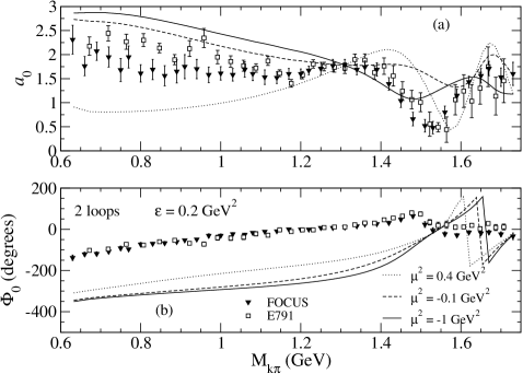
Figure 8: (a) Modulus and (b) phase of the $D^{+}\to K^{-}\pi^{+}\pi^{+}$ S-wave amplitude obtained from Eq. (94). Values for $\mu^{2}$ in GeV²: $0.4$ (dotted line), $-0.1$ (dashed-line), and $-1$ (solid line). The data come from the phase-shift analysis of E791 Aitala12 ; Aitala3 and FOCUS collaboration FOCUS1 ; FOCUS2 .

The fit found in Ref. MagPRD11 below $K^{*}_{0}(1430)$ suggested that the partonic amplitude has little overlap with the $K^{\mp}\pi^{\pm}\pi^{\pm}$ final state channel, i. e., the first term in left-hand-side of Eq. (94) should vanishes. Here, we also show in Fig. 9, results computed only by considering $A_{0}(M^{2}_{K\pi})\approx\tau_{\mbox{\tiny{1/2}}}(M^{2}_{K\pi})\xi^{\mbox{\tiny{3/2}}}_{\mbox{\tiny{3/2,1/2}}}(k_{\pi^{\prime}})$. As in the previous work MagPRD11 , a better fit to the experimental data below $K^{*}_{0}(1430)$ is found, compared to the results showed in Fig. 8. However, note that a structure in the phase is seen in the model which incorporates $K^{*}_{0}(1630)$ and $K^{*}_{0}(1950)$, as also verified in the LASS data. A better fit of the LASS data above $K^{*}_{0}(1430)$ seems necessary to find a better agreement with the valley in the modulus and the structure in the phase, as well. The conclusion is somewhat independent on the subtraction point, at least for those small values given in the figure.

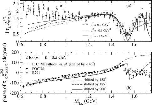
Figure 9: (a) Modulus and (b) phase of $\tau_{\mbox{\tiny{1/2}}}\xi^{\mbox{\tiny{3/2}}}_{\mbox{\tiny{3/2,1/2}}}$. Values for $\mu^{2}$ in GeV²: $0.4$ (dotted line), $-0.1$ (dashed-line), and $-1$ (solid line). For reference, the dotted-dashed line gives the previous covariant calculation up to two-loops from P. C. Magalhães, et. al. of Ref. MagPRD11 . The data come from the phase-shift analysis of E791 Aitala12 ; Aitala3 and FOCUS collaboration FOCUS1 ; FOCUS2 .

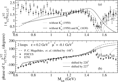
Figure 10: (a) Modulus and (b) phase of $\tau_{\mbox{\tiny{1/2}}}\xi^{\mbox{\tiny{3/2}}}_{\mbox{\tiny{3/2,1/2}}}$ for two cases: i) without $K^{*}_{0}(1950)$ and ii) without $K^{*}_{0}(1950)$ and $K^{*}_{0}(1630)$. Dotted-dashed line: theoretical calculation from P. C. Magalhães, et. al. of Ref. MagPRD11 . Data from the phase-shift analysis of E791 Aitala12 ; Aitala3 and FOCUS collaboration FOCUS1 ; FOCUS2 .

In order to check the effect of the fitting to LASS data above $K^{*}_{0}(1430)$, we remove from the $K\pi$ s-wave amplitude the $K^{*}_{0}(1950)$ and $K^{*}_{0}(1630)$ resonances, as shown in Fig. 10. For this study, we fix the subtraction point at $\mu^{2}=-0.1$ GeV². In the two sets of calculations, we turned off: (i) $K^{*}_{0}(1950)$ (dotted line), (ii) and both $K^{*}_{0}(1950)$ and $K^{*}_{0}(1630)$ (solid line). In case (i), both the structure of the valley in the modulus and phase is somewhat kept, and make distinct the results from Ref. MagPRD11 , while in case (ii) as happens for the reference calculation, the valley and mainly the phase, loose part of their structure. We should note that for calculation (ii), the parameters of $\tau_{\mbox{\tiny{1/2}}}$ were not refitted to the LASS data, and this can be observed by the shift in the valley position of the modulus. Essentially, we restate that the on-shell $K\pi$ amplitude should be represented well in order to compute the rescattering three-body effects. Also, a simple fitting of the low-energy $K\pi$ amplitude without the detailed physics of chiral symmetry, which leads to the broad $\kappa^{*}$ resonance, is somewhat poor below $0.8$ GeV, as the figure suggests.

VII.2 Coupled-channels with $I_{K\pi}=$ 1/2 and 3/2 interactions

We calculated the bachelor amplitudes iterating the coupled equations (79)-(80) and the single channel equation for total isospin $5/2$, Eq. (81), up to two-loops. In this case the amplitude for the s-wave $D^{+}\to K^{-}\pi^{+}\pi^{+}$ decay is written as

$$A_{0}(M^{2}_{K\pi}) = C_{1}\left[\frac{A_{w}}{2}+\tau_{\mbox{\tiny{1/2}}}(M^{2}_{K\pi})\xi^{\mbox{\tiny{3/2}}}_{\mbox{\tiny{3/2,1/2}}}(k_{\pi^{\prime}})\right]+C_{2}\left[\frac{B_{w}}{2}+\tau_{\mbox{\tiny{3/2}}}(M^{2}_{K\pi})\xi^{\mbox{\tiny{3/2}}}_{\mbox{\tiny{3/2,3/2}}}(k_{\pi^{\prime}})\right]+$$ (95)

$$+ C_{3}\left[\frac{C_{w}}{2}+\tau_{\mbox{\tiny{3/2}}}(M^{2}_{K\pi})\xi^{\mbox{\tiny{3/2}}}_{\mbox{\tiny{5/2,3/2}}}(k_{\pi^{\prime}})\right]=a_{0}(M^{2}_{K\pi})e^{i\Phi_{0}(M^{2}_{K\pi})},$$

where the constants $A_{w}$, $B_{w}$ and $C_{w}$ are defined in Eqs. (82). The constants $C_{i}$ are given by

$$C_{1} = \left<K^{-}\pi^{+}\pi^{+}\right|\left.I_{T}=3/2,I_{K\pi}=1/2,I_{T}^{z}=3/2\right>,\qquad$$ (96)

$$C_{2} = \left<K^{-}\pi^{+}\pi^{+}\right|\left.I_{T}=3/2,I_{K\pi}=3/2,I_{T}^{z}=3/2\right>,\qquad$$ (97)

$$C_{3} = \left<K^{-}\pi^{+}\pi^{+}\right|\left.I_{T}=5/2,I_{K\pi}=3/2,I_{T}^{z}=3/2\right>,\qquad$$ (98)

which comes from Eq. (76). The driving terms of the integral equations for $\xi^{I_{T}^{z}}_{I_{T},I_{K\pi}}$, see Eqs. (79)-(81), and the functional form of the amplitude given in Eq. (95), depend on only two free parameters, namely, $W_{1}-W_{2}$ and $W_{3}$. Actually, if we set $W_{3}=0$, there are no free parameters anymore, since $W_{1}-W_{2}$ became an overall constant in the amplitude.

The first striking result is that for $W_{1}=W_{2}$ and $W_{3}$ nonzero, which is also the case for $\left|W\right>=\left|K^{-}\pi^{+}\pi^{+}\right>$ ($W_{i}=1$) is shown in Fig. 11. Only total isospin $5/2$ is allowed and the $K\pi$ pair interacts in isospin $3/2$ state. All the structure in the phase and amplitude is washed out, as the figure shows, excluding that possibility as dominant for the partonic amplitude.

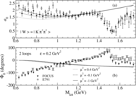
Figure 11: (a) Modulus and (b) phase of the $D^{+}\to K^{-}\pi^{+}\pi^{+}$ amplitude for a initial state with $W_{1}=W_{2}$ and $W_{3}=1$ in Eqs. (90). The data come from the phase-shift analysis of E791 Aitala12 ; Aitala3 and FOCUS collaboration FOCUS1 ; FOCUS2 .

The relevant partonic weight $W_{i}$ should be guided by the difference $W_{1}-W_{2}$, which means dominance of the total isospin $3/2$ in the initial state. In Fig. 12, we present results for $W_{1}=1$ and $W_{2}=W_{3}=0$, which corresponds to a partonic amplitude given by

$$\left|D\right>=\alpha^{\mbox{\tiny{3/2}}}_{\mbox{\tiny{3/2,1/2}}}\left|I_{T}=3/2,I_{K\pi}=1/2,I^{z}_{T}=3/2\right>+\alpha^{\mbox{\tiny{3/2}}}_{\mbox{\tiny{3/2,1/2}}}\left|I_{T}=3/2,I_{K\pi^{\prime}}=1/2,I^{z}_{T}=3/2\right>\ .$$ (99)

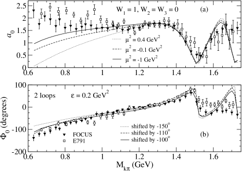
Figure 12: Modulus (a) and phase (b) of the $D^{+}\to K^{-}\pi^{+}\pi^{+}$ amplitude for an initial state with $W_{1}=1$, $W_{2}=W_{3}=0$ in Eqs. (90). The data come from the phase-shift analysis of E791 Aitala12 ; Aitala3 and FOCUS collaboration FOCUS1 ; FOCUS2 .

In the figure, we present results for $\mu^{2}=0.4,-0.1$ and $1$ GeV² and $\epsilon=0.2$ GeV². A reasonable account of the experimental phase and modulus is given by $\mu^{2}=-1$ GeV² and $\mu^{2}=-0.1$ GeV². At low $M_{K\pi}$ below 1 GeV, the model does not describe the modulus, where the different analysis of E791 and FOCUS present a large dispersion. The model tends to underestimate the modulus in the low mass region. The bachelor amplitude increases with $M_{K\pi}$ (see e.g. Fig. 7), which leads model to underestimate the modulus of the decay amplitude for low $K\pi$ masses. The characteristics valley and the follow-up height is somewhat described by the model, with exception of the region close to the boundary of the decay phase-space, where the data seems to indicates an increase of the amplitude and the model presents a noticeable decrease.

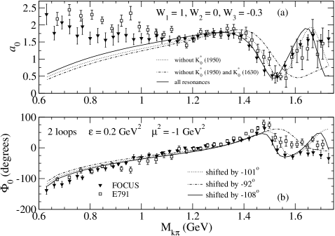
Figure 13: (a) Modulus and (b) phase of the $D^{+}\to K^{-}\pi^{+}\pi^{+}$ amplitude for two cases: i) without $K^{*}_{0}(1950)$ and ii) without $K^{*}_{0}(1950)$ and $K^{*}_{0}(1630)$. In all cases we considered $W_{1}=1$, $W_{2}=0$ and $W_{3}=-0.3$. The data come from the phase-shift analysis of E791 Aitala12 ; Aitala3 and FOCUS collaboration FOCUS1 ; FOCUS2 .

We performed variations of the weight parameters and verified that a small mixture of total isospin $5/2$ improves the fittings. We have used $W_{1}=1$, $W_{2}=0$ and $W_{3}=-0.3$ to obtain the results shown by the solid lines in Fig. 13 for $\mu^{2}=-1$ GeV². Notice also that the effect of the resonances in the fit of the $K\pi$ isospin $1/2$ amplitude to the LASS data, in the last model results, is similar to the single channel case we have already discussed. The region close to the valley appearing in the modulus is sensitive mainly to our fit of the LASS data in the neighborhood of $K^{*}_{0}(1630)$, while $K^{*}_{0}(1950)$ presents a smaller effect in part due to the competition with the interaction in the $I_{K\pi}=3/2$ state. The pronounced minimum in the modulus of the decay amplitude, which appears in the $D-$decay phase-shift data at 1.53 GeV, should be contrasted with the LASS phase-shift in Fig.  1, where the deep in not well pronounced and placed at 1.65 GeV.

VIII Summary and Conclusions

We have investigated the three-body final state interaction effects in $D^{+}$ decays focusing in the $K^{-}\pi^{+}\pi^{+}$ channel. In order to formulate the final state interaction contribution to the decay, we used a relativistic three-body model for the final state interaction in a heavy meson decay based on an approximation of the Bethe-Salpeter-Faddeev equations proposed in Ref. MagPRD11 and generalized to include different isospin channels of the interacting pair. The numerical calculations were performed in three-dimensions, corresponding to the projection of the Bethe-Salpeter like equations for the Faddeev components of decay amplitude to the light-front. We generalized the quasi-potential approach applied to the light-front projection of the Bethe-Salpeter equation to account for the three-body final state interaction in heavy-meson decays. The calculations were performed with a truncated light-front equation to the valence states and rotational symmetry was putted under control. The particular kinematics of the decay in three-mesons, allows to choose the transverse plane as the decay plane. This particular rotation around the z-direction is of kinematical nature and therefore preserved by the truncation of the Fock-space.

The $K\pi$ S-wave amplitude model is fitted to the LASS data for isospin $1/2$, including the resonances $K^{*}_{0}(1430)$, $K^{*}_{0}(1630)$ and $K^{*}_{0}(1950)$. The isospin $3/2$ amplitude is taken from an effective range formula already presented in Ref. LASS . We allowed the partonic amplitude to have nonzero weight in the three possible isospin states with $I_{T}$ equal to 3/2 and 5/2. A small contribution of $I_{T}=5/2$ seems to improve the fit of the data of amplitude and phase from E791 Aitala12 ; Aitala3 and FOCUS FOCUS1 ; FOCUS2 collaborations.

We showed that the loop-expansion to calculate three-body rescattering effects in the $K\pi\pi$ channel converges fast, and the solution of the integral equations for the bachelor amplitudes by iteration at the three-loop level gives a contribution that can be neglected in respect to the two-loop results. We explored the dependence on the model parameters in respect to the partonic amplitude.

We found that the negative value of the phase seen in the data Aitala12 ; Aitala3 ; FOCUS1 ; FOCUS2 , can be obtained by an appropriate choice of the real weights of the three isospin components of the partonic amplitude, with a small mixture of total isospin 5/2. The feature of the modulus of the unsymmetrized decay amplitude presenting a deep valley and a following increase, for $K\pi$ masses above 1.5 GeV, is fairly reproduced, which indicates an assignment of $0^{+}$ to the isospin 1/2 $K^{*}(1630)$ PDG omitted from the PDG summary table. Below 1 GeV the model underestimate the data for the modulus, as happens close to the end of the available phase-space around 1.8 GeV.

Certainly, a better comprehension of the $K\pi$ amplitude in the physical and unphysical region, and in particular above $K^{*}(1430)$ can bring more realism to the description of the three-body final state interaction in $D$ decays. The challenge of applying the formalism to $B$ decays and CP violation LHCb1 by extending Ref. CPT to include three-body FSI, is let to a future work.

- (1) I. I. Bigi, A. I. Sanda, CP Violation (Cambridge University Press, Cambridge, England, 2009), Ed. 2.
- (2) M. Sozzi, Discrete Symmetries and CP Violation From Experiment to Theory (Oxford University Press, New York, 2008).
- (3) M. Kobayashi and T. Maskawa, CP Violation in the Renormalizable Theory of Weak Interaction, Prog. Theor. Phys. 49 (1973) 652.
- (4) K. Nakamura et al. [Particle Data Group Collaboration], Review of particle physics, J. Phys. G37 (2010) 075021.
- (5) S. Bianco, F. L. Fabbri, D. Benson and I. Bigi, A Cicerone for the physics of charm, Riv. Nuovo Cim. 26N7 (2003) 1 [hep-ex/0309021].
- (6) E. M. Aitala et al. [E791 Collaboration], Study of the decay and measurement of masses and widths, Phys. Rev. Lett. 86 (2001) 765 [hep-ex/0007027].
- (7) E. M. Aitala et al. [E791 Collaboration], Dalitz plot analysis of the decay and indication of a low-mass scalar resonance, Phys. Rev. Lett. 89 (2002) 121801 [hep-ex/0204018].
- (8) J. M. Link et al. [FOCUS Collaboration], Dalitz plot analysis of and decay to using the K matrix formalism, Phys. Lett. B585 (2004) 200 [hep-ex/0312040].
- (9) J. M. Link et al. [FOCUS Collaboration], The S-wave from the decay, Phys. Lett. B681 (2009) 14 [arXiv:0905.4846 [hep-ex]].
- (10) G. Bonvicini et al. [CLEO Collaboration], Dalitz plot analysis of the decay, Phys. Rev. D78 (2008) 052001 [arXiv:0802.4214 [hep-ex]].
- (11) D. Aston, N. Awaji, T. Bienz, F. Bird, J. D’Amore, W. M. Dunwoodie, R. Endorf and K. Fujii et al., A Study of Scattering in the Reaction at 11-GeV/c, Nucl. Phys. B296 (1988) 493.
- (12) R. H. Dalitz, On the analysis of tau-meson data and the nature of the tau-meson, Phil. Mag. 44 (1953) 1068.
- (13) J. Adler et al. [MARK-III Collaboration], Resonant Substructure in K pi pi Decays of Charmed d Mesons, Phys. Lett. B196 (1987) 107.
- (14) J. Adler et al. [MARK-III Collaboration], A Reanalysis of Charmed d Meson Branching Fractions, Phys. Rev. Lett. 60 (1988) 89.
- (15) J. Adler et al. [Mark-III Collaboration], Resonant Substructure in Decays of D0 Mesons, Phys. Rev. Lett. 64 (1990) 2615.
- (16) J. Adler et al. [MARK-III Collaboration], Upper Limit on the Absolute Branching Fraction for , Phys. Rev. Lett. 64 (1990) 169.
- (17) M. P. Alvarez et al. [NA14/2 Collaboration], Measurement of and Cabibbo suppressed decays, Phys. Lett. B246 (1990) 261.
- (18) M. P. Alvarez et al. [NA14/2 Collaboration], Branching ratios and properties of D meson decays, Z. Phys. C50 (1991) 11.
- (19) J. C. Anjos, J. A. Appel, A. Bean, S. B. Bracker, T. E. Browder, L. M. Cremaldi, J. R. Elliott and C. O. Escobar et al., Measurement of and Decays to Nonstrange States, Phys. Rev. Lett. 62 (1989) 125.
- (20) J. C. Anjos et al. [E691 Collaboration], A Dalitz plot analysis of decays, Phys. Rev. D48 (1993) 56.
- (21) P. L. Frabetti et al. [E687 Collaboration], A Measurement of ), Phys. Lett. B313 (1993) 253.
- (22) P. L. Frabetti et al. [E687 Collaboration], Analysis of the , Dalitz plots, Phys. Lett. B407 (1997) 79.
- (23) E. M. Aitala et al. [E791 Collaboration], Model independent measurement of S-wave systems using decays from Fermilab E791, Phys. Rev. D73 (2006) 032004 [Erratum-ibid. D74 (2006) 059901] [hep-ex/0507099].
- (24) A. C. dos Reis, The Kpi and pipi S-wave from D decays, contribution to the CHARM09 Proceedings, Leimen, Germany.
- (25) K. M. Watson, The Effect of final state interactions on reaction cross-sections, Phys. Rev. 88 (1952) 1163.
- (26) P. C. Magalhães, M. R. Robilotta, K. S. F. F. Guimaraes, T. Frederico, W. de Paula, I. Bediaga, A. C. d. Reis and C. M. Maekawa et al., Towards three-body unitarity in , Phys. Rev. D84 (2011) 094001 [arXiv:1105.5120 [hep-ph]].
- (27) D. R. Boito and R. Escribano, Kpi form-factors and final state interactions in decays, Phys. Rev. D80 (2009) 054007 [arXiv:0907.0189 [hep-ph]].
- (28) D. R. Boito and R. Escribano, K pi form factors, final state interactions and decays, AIP Conf. Proc. 1257 (2010) 370 [arXiv:1003.5232 [hep-ph]].
- (29) K. S. F. F. Guimaraes, I. Bediaga, A. Delfino, T. Frederico, A. C. dos Reis and L. Tomio, Three-body model of the final state interaction in heavy meson decay, Nucl. Phys. Proc. Suppl. 199 (2010) 341.
- (30) T. Frederico, K. S. F. F. Guimaraes, W. de Paula, I. Bediaga, A. C. dos Reis, P. C. Magalhaes, M. Robilotta and A. Delfino et al., Relativistic three-body model for final state interaction in decay, PoS LC 2010 (2010) 005.
- (31) J. H. O. Sales, T. Frederico, B. V. Carlson and P. U. Sauer, Light front Bethe-Salpeter equation, Phys. Rev. C61 (2000) 044003 [nucl-th/9909029].
- (32) J. A. O. Marinho, T. Frederico and P. U. Sauer, Light-front Ward-Takahashi identity and current conservation, Phys. Rev. D76 (2007) 096001.
- (33) J. A. O. Marinho and T. Frederico, Next-to-leading order light-front three-body dynamics, PoS LC 2008 (2008) 036.
- (34) J. A. O. Marinho, T. Frederico and P. U. Sauer, Ward-Takahashi identity for the electromagnetic current of two-particle systems on the light front, Few Body Syst. 44 (2008) 307.
- (35) J. A. O. Marinho, T. Frederico, E. Pace, G. Salme and P. Sauer, Light-front Ward-Takahashi Identity for Two-Fermion Systems, Phys. Rev. D77 (2008) 116010 [arXiv:0805.0707 [hep-ph]].
- (36) T. Frederico and G. Salme, Projecting the Bethe-Salpeter Equation onto the Light-Front and back: A Short Review, Few Body Syst. 49 (2011) 163 [arXiv:1011.1850 [nucl-th]].
- (37) T. Frederico, K. S. F. F. Guimaraes, O. Lourenco, W. de Paula, I. Bediaga and A. C. d. Reis, Heavy meson decay in three-mesons and FSI, arXiv:1402.6975 [hep-ph].
- (38) J. Carbonell, B. Desplanques, V. A. Karmanov and J. F. Mathiot, Explicitly covariant light front dynamics and relativistic few body systems, Phys. Rept. 300 (1998) 215 [nucl-th/9804029].
- (39) S. J. Brodsky, H. -C. Pauli and S. S. Pinsky, Quantum chromodynamics and other field theories on the light cone, Phys. Rept. 301 (1998) 299 [hep-ph/9705477].
- (40) B. L. G. Bakker, L. A. Kondratyuk and M. V. Terentev, On The Formulation Of Two-body And Three-body Relativistic Equations Employing Light Front Dynamics, Nucl. Phys. B158 (1979) 497.
- (41) M. G. Fuda, Covariant Time Ordered Perturbation Theory, Phys. Rev. C33 (1986) 996.
- (42) T. Frederico, Null plane model of three bosons with zero range interaction, Phys. Lett. B282 (1992) 409.
- (43) S. K. Adhikari, T. Frederico and L. Tomio, Relativistic three particle dynamical equations. 1. Theoretical development, Annals Phys. 235 (1994) 77 [nucl-th/9311035].
- (44) J. Carbonell and V. A. Karmanov, Three boson relativistic bound states with zero range interaction, Phys. Rev. C67 (2003) 037001 [nucl-th/0207073].
- (45) J. Beringer et al. [Particle Data Group Collaboration], Review of Particle Physics (RPP), Phys. Rev. D86 (2012) 010001.
- (46) W. de Paula and T. Frederico, Scalar mesons within a dynamical holographic QCD model, Phys. Lett. B693 (2010) 287 [arXiv:0908.4282 [hep-ph]].
- (47) W. de Paula and T. Frederico, Scalar Spectrum from a Dynamical Gravity/Gauge model, Int. J. Mod. Phys. D19 (2010) 1351 [arXiv:1004.0709 [hep-ph]].
- (48) W. de Paula, T. Frederico, H. Forkel and M. Beyer, Dynamical AdS/QCD with area-law confinement and linear Regge trajectories, Phys. Rev. D79 (2009) 075019 [arXiv:0806.3830 [hep-ph]].
- (49) P. Masjuan, E. Ruiz Arriola and W. Broniowski, Systematics of radial and angular-momentum Regge trajectories of light non-strange -states, Phys. Rev. D85 (2012) 094006 [arXiv:1203.4782 [hep-ph]].
- (50) B. Aubert et al. [BaBar Collaboration], Time-dependent amplitude analysis of B0 —¿ K0(S) pi+ pi-, Phys. Rev. D80 (2009) 112001 [arXiv:0905.3615 [hep-ex]].
- (51) P. Estabrooks, R. K. Carnegie, A. D. Martin, W. M. Dunwoodie, T. A. Lasinski and D. W. G. S. Leith, Study of K pi Scattering Using the Reactions and at 13-GeV/c, Nucl. Phys. B133 (1978) 490.
- (52) V. A. Karmanov and P. Maris, Manifestation of three-body forces in three-body Bethe-Salpeter and light-front equations, Few Body Syst. 46 (2009) 95 [arXiv:0811.1100 [hep-ph]].
- (53) P. C. Magalhães and M. C. Birse, A model for final state interactions in D+ —¿ K- pi+ pi+, PoS QNP 2012 (2012) 144.
- (54) R. Aaij et al. [LHCb Collaboration], Measurement of CP violation in the phase space of and decays, Phys. Rev. Lett. 111 (2013) 101801 [arXiv:1306.1246 [hep-ex]].
- (55) I. Bediaga, T. Frederico and O. Lourenço, CP violation and CPT invariance in decays with final state interactions, arXiv:1307.8164 [hep-ph].