Unlearning Quantum Information

Abstract

Quantum dynamics can be driven by measurement. By constructing measurements that gain no information, effective unitary evolution can be induced on a quantum system, for example in ancilla driven quantum computation. In the non-ideal case where a measurement does reveal some information about the system, it may be possible to “unlearn” this information and restore unitary evolution through subsequent measurements. Here we analyse two methods of quantum “unlearning” and present a simplified proof of the bound on the probability of successfully applying the required correction operators. We find that the probability of successful recovery is inversely related to the ability of the initial measurement to exclude the possibility of a state.

I Introduction

In quantum information processing schemes such as measurement-based quantum computation MBQC2003 , ancilla-driven quantum computation Twisted2009 ; ADQC2010 ; Twisted2012 , and holonomic degenerate projections AP1989 ; Oi2014 , unitary quantum dynamics are driven by measurements that learn nothing about the system. Previous work has studied several issues including non-ideal coupling between system and ancilla MK2010 , preparation, gate, storage and measurement errors RHG2007 . Here, we address the issue of “unlearning” information gained from a non-ideal generalized measurement by subsequent conditional measurements to restore the unitary evolution of the system. This question has been addressed before in the context of reversing measurement UIN1996 ; KU1999 ; ParaoanuPRA2011 ; CL2012 , experimental proposals KJ2006 ; JK2010 ; ParaoanuEPL2011 and demonstrations Katz2008 ; Kim2009 . We present a simplified proof of the bound on the success probability of such corrective measures and relate it to the spectrum of the measurement operators corresponding to non-unitary evolution as well as describing finite and asymptotic correction schemes achieving this limit.

II Preliminaries

A generalized measurement, or positive operator valued measure (POVM), can be described by a set of positive operators $\{M_{j}\}$ that sum to the identity, $\sum_{j}M_{j}=\mathbb{I}$. The probability of obtaining outcome $j$ when measuring system described by density operator $\rho$ is $p_{j}=\text{Tr}[M_{j}\rho]$. The post-measurement state is not uniquely defined by $M_{j}$ in general, but is given by $\rho_{j}=\frac{K_{j}\rho K_{j}^{\dagger}}{\text{Tr}[K_{j}^{\dagger}K_{j}\rho]}$ where $M_{j}=K_{j}^{\dagger}K_{j}$, and $\{K_{j}\}$ are Kraus operators. In this paper, we will always consider the post-measurement state to be of the same dimensionality as the input.

Figure 1: Two-level binary POVM tree. Each bifurcation represents a binary POVM with two Kraus operators labeling the arrows. The nodes of the tree represent the cumulative measurement operator corresponding to the sequence of results leading to that node. The cumulative Kraus operator consists of the product of all the Kraus operators along the path down the branch. The sum of the $\tilde{M}$ children of a branch sum up to parent node.

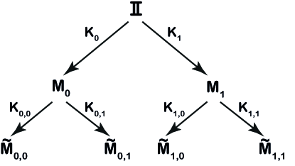
A cascaded sequence of measurements (Fig. 1) results in a cumulative Kraus operator that is the product of the individual Kraus operators associated with each sequential result, e.g. if a first measurement has Kraus operators $\{K_{j}\}$, and depending on the result $j$, a second measurement is performed with Kraus operators $\{K_{j,k}\}$, the total Kraus operator associated with joint result $j$ and then $k$ is given by $\tilde{K}_{j,k}=K_{j,k}K_{j}$, and the POVM element is given by $\tilde{M}_{j,k}=(\tilde{K}_{j,k})^{\dagger}\tilde{K}_{j,k}$.

We will consider the case where ideally we would like the Kraus operators to be proportional to a unitary, $K_{j}=q_{j}U_{j}$ where $0<q_{j}\leq 1$ for some unitary $U_{j}$. This results in $M_{j}=q_{j}^{2}\mathbb{I}$, hence the measurement probabilities are independent of $\rho$, i.e. obtaining outcome $j$ reveals no information about the state of the system. This ensures that $\rho_{j}=U_{j}\rho U_{j}^{\dagger}$.

In ADQC Twisted2009 ; ADQC2010 ; Twisted2012 , the coupling and measurement of a ancilla qubit to the system results in a two-outcome POVM where the alternative Kraus operators are unitary and are related by a Pauli correction. This requires the coupling between system and ancilla to be of a special form, and that the ancilla qubit be prepared and measured in particular directions ADQC2010 . Should this not be the case, then the effective Kraus operators may not result in the desired unitary conditional evolution but may reveal information about the system.

Without loss of generality, we may just consider two-outcome POVMs since a multiple outcome POVM can be considered as the result of multiple cascaded two-outcome POVMS AO2008 . Using the singular value decomposition, we can ignore the unitary transformations and only consider the singular values which encode the (non)unitary properties of the operator DBN2013 .

The question we will answer is thus, given an initial POVM with Kraus operators whose singular values are not equal, how can we perform subsequent operations so that at least some of the outcomes result in conditional unitary evolution of the initial state, and what is the maximum probability of such corrective action?

We show that simple filtering or procrustean operations are sufficient to “equalize” the cumulative singular values and thus unlearn the information gained in prior steps. The maximum probability of enacting conditional unitary evolution after an initial information-gaining binary outcome measurement is related to the spectral width, i.e. the difference between the largest and smaller singular values of the Kraus operators.

III Procrustean Filtering

We shall show how we can correct an initial non-unitary inducing measurement by a filtering operation similar to that used for entanglement concentration Procrust1996 . Let us assume that after the first measurement, we obtain the outcome associated with Kraus operator $K_{0}=\text{diag}(q_{0}^{k})$ where the $q_{0}^{k}$ are not all the same. The probability of this result is $p_{0}=\text{Tr}[K_{0}^{\dagger}K_{0}\rho]$ and varies from $(q_{0}^{k_{min}})^{2}\leq p_{0}\leq(q_{0}^{j_{max}})^{2}$. Since the probability depends on the state, we gain information through this measurement and the state evolves non-unitarily.

We now try to correct the evolution with another measurement with diagonal Kraus operators $K_{0,j}=\text{diag}(q_{0,j}^{k}),\;j=0,1$ resulting in the conditional cumulative Kraus operators, $K_{0,j}K_{0}=\text{diag}(q_{0,j}^{k}q_{0}^{k})$. We can choose the singular values so that for one of the outcomes, the resultant evolution is restored to being unitary.

Let us choose $K_{0,0}$ to correct $K_{0}$. If $q_{0}^{k_{min}}$ is the smallest singular value of $K_{0}$, then setting $q_{0,0}^{k}=q_{0}^{k_{min}}/q_{0}^{k}$ results in the cumulative operation $K_{0,0}K_{0}=q_{0}^{k_{min}}\mathbb{I}$. The other outcome $K_{0,1}$ will have at least one vanishing singular value, hence will have a non-trivial nullspace and it will be impossible to further correct this branch of the measurement tree. The probability of arriving at $\tilde{K}_{0,0}=q_{0}^{k_{min}}\mathbb{I}$ is $p_{0,0}=(q_{0}^{k_{min}})^{2}$ independent of the initial state as required.

If at the first measurement we obtained the complementary result $K_{1}=\text{diag}(q_{1}^{k})$, then a subsequent correction would result in outcome $\tilde{K}_{1,1}=q_{1}^{k_{min}}\mathbb{I}$ with probability $p_{1,1}=(q_{1}^{k_{min}})^{2}$. The completeness of the measurement operators implies that $(q_{1}^{k_{min}})^{2}=1-(q_{0}^{k_{max}})^{2}$, hence the total probability of a successful correction after the initial measurement is $p_{tot}=1-[(q_{0}^{k_{max}})^{2}-(q_{0}^{k_{min}})^{2}]$, or one minus the visibility.

We can generalize the result to the case where the first measurement has more than two outcomes. In this case, the probability of successful correction is given by $p_{tot}=\sum_{j}(q_{j}^{k_{min}})^{2}$. Hence the uncorrectable non-unitary action of the initial measurement is determined by how much an outcome excludes a state compared with others.

IV Partial Filtering

Figure 2: Partial Filtering. Instead of succeeding or failing outright after one step, we can partially filter out corrected portions of the evolution, represented by the paths leading out to the sides. The vertical downward arrows represent partial failures, upon which we can retry recovery. The failure probability is given by the sum of the limiting residual cumulative measurement operators, $p_{fail}\mathbb{I}=\tilde{M}_{\infty}^{0}+\tilde{M}_{\infty}^{1}$.

We saw in the above section that we can choose our corrective measurements to either succeed, or fail entirely with no further recourse. An alternate strategy would be to succeed on one outcome, but the alternative could still be further correctable. We shall illustrate this in the case of a single qubit system.

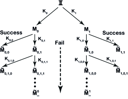
Let the initial binary outcome measurement have Kraus operators, $K_{0}=\text{diag}(a,b)$ and $K_{1}=\sqrt{\mathbb{I}-K_{0}^{\dagger}K_{0}}$ where $0<b<a<1$. Suppose that we obtain outcome $K_{0}$, we can choose to correct the evolution using the method in the previous section or else we can choose, for example, the operators $K_{0,0}=\text{diag}(b,a)$ and $K_{0,1}=\sqrt{\mathbb{I}-K_{0,0}^{\dagger}K_{0,0}}$. In the case of the result $K_{0,0}$, we achieve the cumulative evolution $\tilde{K}_{0,0}=ab\mathbb{I}$, but the unsuccessful outcome $\tilde{K}_{0,1}$ still has full rank and could be further processed. The situation reduces to that of before but with a new effective Kraus operator $\tilde{K}_{0,1}=\text{diag}(a^{(1)}=a\sqrt{1-b^{2}},b^{(1)}=b\sqrt{1-a^{2}})$ and we can try to apply another round of corrections (Fig. 2).

This gives a recursive formula for the success probability for the $K_{0}$ branch,

$$p_{tot}^{2}=\sum_{j}p_{j}^{0},\quad p_{j}^{0}=\left(a^{(j)}b^{(j)}\right)^{2}$$

$$a^{(j+1)}=a^{(j)}\sqrt{1-{b^{(j)}}^{2}},\quad b^{(j+1)}=b^{(j)}\sqrt{1-{a^{(j)}}^{2}},$$ (1)

and for the $K_{1}$ branch,

$$p_{tot}^{1}=\sum_{j}p_{j}^{1},\quad p_{j}^{1}=\left(c^{(j)}d^{(j)}\right)^{2}$$

$$c^{(j+1)}=c^{(j)}\sqrt{1-{d^{(j)}}^{2}},\quad d^{(j+1)}=d^{(j)}\sqrt{1-{c^{(j)}}^{2}},$$ (2)

where $c=\sqrt{1-a^{2}}$ and $d=\sqrt{1-b^{2}}$, and $a^{(0)}=a$ etc. It is simple to check that $a^{(j)}=d^{(j)}$ and $b^{(j)}=c^{(j)}$ $\forall j\geq 1$.

In order to compute the limiting value of the success probability, it is easier to compute the probability of failure. This can be found by finding the limit of the unsuccessful Kraus operators given by

$$\tilde{K}_{\infty}^{0}=\text{diag}(a^{(\infty)},b^{(\infty)}),\quad\tilde{K}_{\infty}^{1}=\text{diag}(c^{(\infty)},d^{(\infty)}),$$ (3)

and the total failure probability is

$$p_{fail}\mathbb{I}=\tilde{M}_{\infty}^{0}+\tilde{M}_{\infty}^{1}=\left({a^{(\infty)}}^{2}+{b^{(\infty)}}^{2}\right)\mathbb{I},$$ (4)

where $\tilde{M}_{\infty}^{0,1}=(\tilde{K}_{\infty}^{0,1})^{\dagger}\tilde{K}_{\infty}^{0,1}$

To solve the recursion formula, we first note that ${a^{(j+1)}}^{2}-{b^{(j+1)}}^{2}={a^{(j)}}^{2}-{b^{(j)}}^{2}=a^{2}-b^{2}$. We also note that the fixed points of the recursion relation are when $b^{(\infty)}=0$ leading to the limit

$$K_{\infty}^{0}=\text{diag}(a^{2}-b^{2},0),\quad K_{\infty}^{1}=\text{diag}(0,a^{2}-b^{2}),$$ (5)

hence $p_{fail}=a^{2}-b^{2}$, conversely $p_{tot}=1-(a^{2}-b^{2})$, the same as for the Procrustean method.

V Success Bound

We show that the Procrustean method achieves the maximum probability of success. In general, assume that at some stage of the measurement tree the effective Kraus operator is given by $K_{j}=\text{diag}(q_{j}^{k})$. Any corrective set of Kraus operators has to satisfy $\mathbb{I}=\sum_{k}K_{j,k}^{\dagger}K_{j,k}$ which implies that

$$\sum_{k}\tilde{K}_{j,k}^{\dagger}\tilde{K}_{j,k}=K_{j}^{\dagger}K_{j},$$ (6)

where $\tilde{K}_{j,k}=K_{j,k}K_{j}$ is the cumulative Kraus operator for the outcome $k$.

If we consider all branches $k^{\prime}$ that result in conditional unitary evolution, then these add up to $\sum_{k\in\{k^{\prime}\}}\tilde{K}_{j,k}^{\dagger}\tilde{K}_{j,k}=p_{j}^{succ}\mathbb{I}$, hence the branches that do not succeed sum to $K_{j}^{\dagger}K_{j}-p_{j}^{succ}\mathbb{I}$. As this has to be a positive operator, $p_{j}^{succ}$ cannot be larger than the square of the minimum singular value of $K_{j}$. The procrustean method saturates this bound. We note that this result is independent of the use of the singular value decomposition (one may work just with the measurement operators) hence encompasses any general set of correction Kraus operators, not just those “aligned” with the bases of previous results.

When considering all of the initial branches of an non-ideal measurement $\{M_{j}\}$, the maximum total probability of recovery is given by $\sum_{j}p_{j}^{min}$ where $p_{j}^{min}$ is the minimum probability to obtain outcome $j$ when taken over all possible input states. Measurement operators of the form $M_{j}=q_{j}^{2}(\mathbb{I}-|\psi_{j}\rangle\langle\psi_{j}|)$ reveal little information, especially as the dimensionality of the space increases, but are not recoverable.

VI Application to probabilistic teleportation

We apply the results to the well studied problem of probabilistic quantum teleportation as an illustration. Alice and Bob share a non-maximally entangled state of the form $|\Psi(\theta)\rangle=\cos\frac{\theta}{2}|00\rangle+\sin\frac{\theta}{2}|11\rangle$ where $0\leq\theta\leq\pi/2$. Charlie gives Alice a qubit in the state $|\phi\rangle=\alpha|0\rangle+\beta|1\rangle$ to teleport to Bob with the proviso that it either arrives with unit fidelity, or else it fails. The standard solution AP2002 is for Alice to measure in a non-maximally entangled basis,

$$|\Psi^{(0)}\rangle = \sin\frac{\theta}{2}|00\rangle+\cos\frac{\theta}{2}|11\rangle$$

$$|\Psi^{(1)}\rangle = \sin\frac{\theta}{2}|10\rangle+\cos\frac{\theta}{2}|01\rangle$$

$$|\Psi^{(2)}\rangle = \cos\frac{\theta}{2}|00\rangle-\sin\frac{\theta}{2}|00\rangle$$

$$|\Psi^{(3)}\rangle = \cos\frac{\theta}{2}|10\rangle-\sin\frac{\theta}{2}|01\rangle.$$ (7)

The first two outcomes will be obtained each with probability $\frac{1}{4}\sin^{2}\theta$ and result in (reversible) unitary quantum channels between Alice and Bob.

For the other two results, Alice obtains some information about Charlie’s state resulting in operations with singular values $\{\cos^{2}\frac{\theta}{2},\sin^{2}\frac{\theta}{2}\}$. Bob can choose to reverse the non-unitary dynamics by filtering with probability $\sin^{4}\frac{\theta}{2}$ in both cases. The total probability of Alice and Bob to succeed in teleporting $|\phi\rangle$ is $p=2\left(\frac{1}{4}\sin^{2}\theta\right)+2\left(\sin^{2}\frac{\theta}{2}\right)^{2}=1-\cos\theta$. This recovery is optimal as it matches the sums of the squares of the minimal singular values of the initial $4$-outcome POVM on $|\phi\rangle$. We note that this probability matches that of initially filtering $|\Psi(\theta)\rangle$ to obtain a maximally entangled state prior to conventional teleportation.

VII Conclusion and Discussion

These results answer a question about general binary measurement trees and the form that they can take AO2008 . The extension of the success bound to arbitrary measurement trees implies that trees with all the final operators conditionally unitary cannot have any non-unitary branch within it. This places strong constraints on the allowed couplings in ADQC-like architectures as all ancilla-driven dynamics much be unitary to maintain the continuing coherence of the register Oi2014 . Even relaxing the requirement for determinism SO2013A , the Cartan decomposition of the system-ancilla interaction must remain rank deficient, i.e. not of the SWAP form Cartan2003 .

The maximum probability of recovery takes on a simple form when restricted to a binary outcome POVM, being the one minus the difference between the maximum and minimum measurement probabilities. In the case of a multiple outcome POVM, it becomes the sum of the minimum probabilities of each measurement operator.

The results presented recreate those given in Refs. KU1999 and CL2012 but we make minimal reference to states, the emphasis here is entirely on the Kraus operators and elements of the effective POVM. In this way, the proof presented in Sec. V is considerably shortened and simplified compared with previous papers. Also in contrast, instead of information gain in terms of estimation fidelity, the results suggest that reversibility is better characterized by the ability to discount the possibility of a state or subspace BJOP2014 . For example in the continuous variable case, an overcomplete POVM with uncountably many elements all that are proportional to $\mathbb{I}-|\alpha\rangle\langle\alpha|$ ($|\alpha\rangle$ is a coherent state) OPJ2013 , would reveal little information about an input state, but would not be reversible for any of its outcomes.