Reconstruction of the primordial power spectra with Planck and BICEP2
Abstract
By using the cubic spline interpolation method, we reconstruct the shape of the primordial scalar and tensor power spectra from the recently released Planck temperature and BICEP2 polarization cosmic microwave background data. We find that the vanishing scalar index running () model is strongly disfavored at more than confidence level on the Mpc-1 scale. Furthermore, the power-law parameterization gives a blue-tilt tensor spectrum, no matter using only the first 5 bandpowers or the full 9 bandpowers of BICEP2 data sets. Unlike the large tensor-to-scalar ratio value () under the scale-invariant tensor spectrum assumption, our interpolation approach gives by using the first 5 bandpowers of BICEP2 data. After comparing the results with/without BICEP2 data, we find that Planck temperature with small tensor amplitude signals and BICEP2 polarization data with large tensor amplitude signals dominate the tensor spectrum reconstruction on the large and small scales, respectively. Hence, the resulting blue tensor tilt actually reflects the tension between Planck and BICEP2 data.
I Introduction
Recently BICEP2 experiment Ade:2014xna reported an excess of Cosmic Microwave Background (CMB) B-mode polarization power spectrum over the base lensed-CDM expectation in the range , inconsistent with the null hypothesis at a significance of . Since the single field slow-roll inflationary model predicts a peak around multipole in the B-mode auto-correlation (BB) spectrum seeded by the primordial gravitational wave/tensor perturbation mode, the BICEP2 results are believed as the first indirect detection of the primordial gravitational wave. Under the assumption of power-law scalar and scale-invariant tensor spectra, the observed B-mode power spectrum is well-described by a lensed-CDM+tensor theoretical model with tensor-to-scalar ratio with disfavored at confidence level.
However, the scientific results of BICEP2 data are in tension with those from other CMB experiments, such as Planck Ade:2013uln . The first discrepancy is in the amplitude of the scale-invariant tensor spectrum, which is described by the tensor-to-scalar ratio . Unlike the scalar perturbatoins, due to the absence of acoustic oscillation mechanism the tensor contributions to the temperature CMB spectrum are rapidly washed out inside the horizon at electron-proton recombination epoch () Hu:1997hp . Hence, the temperature anisotropies on the large scales are the mixture of scalar and tensor contributions. Furthermore, if one assumes the simple power-law form of the primordial scalar power spectrum, i.e., no scalar index running , the precisely measured higher multipoles by Planck put stringent constraints on the scalar amplitude and index . Therefore, in order to explain the observed power deficit in the low- regime by Planck, one has to suppress the tensor spectrum amplitude. Consequently, from only the temperature anisotropy measured by Planck, one has at , which is in a “very significant” tension (around unlikely) with BICEP2 results Smith:2014kka . As stressed by the BICEP2 team, however, this tension could be reconciled by adding the running of the scalar index which is the degree of freedom to suppress the scalar temperature anisotropy in low- regime. Then, combining Planck with WMAP low- polarization Hinshaw:2012aka and ACT Das:2013zf /SPT Keisler:2011aw ; Story:2012wx ; Reichardt:2011yv high- data, one could get at . Besides that, several other possible solutions to this tension have been proposed, such as step feature spectra Bousso:2014jca ; Miranda:2014wga ; Hazra:2014aea , fast-slow roll model Hazra:2014jka , anti-correlation scalar iso-curvature initial condition Kawasaki:2014lqa ; Kawasaki:2014fwa , sterile neutrino species Giusarma:2014zza ; Zhang:2014dxk ; Dvorkin:2014lea , sudden change in speed of inflaton or Lorentz violation Contaldi:2014zua . And see also Freivogel:2014hca ; Firouzjahi:2014fda ; Cai:2014bda ; Cheng:2014bta ; Choudhury:2014kma ; Hotchkiss:2011gz for other possibilities.
The second tension is between the observed blue-tilt tensor spectrum () Gerbino:2014eqa ; Wu:2014qxa ; Cheng:2014ota ; Li:2014cka ; Chang:2014loa by BICEP2 and the red-tilt one () predicted by the standard inflationary paradigm. Generally, the blue tensor spectrum asks for violation of Null Energy Condition (NEC), which is equivalent to (or ) in the flat universe. There exist several NEC violation inflationary models in the literature, such as super-inflation Baldi:2005gk , phantom inflation Piao:2004tq , G-inflation Kobayashi:2010cm etc. Some alternative paradigm of inflation, such as “string gas cosmology” Brandenberger:2014faa , bouncing universe Creminelli:2006xe ; Creminelli:2007aq ; Buchbinder:2007ad ; Xia:2014tda ; Qiu:2014nla ; Piao:2003zm ; Liu:2013kea or other possibilities Gong:2014qga ; Wang:2014kqa (see the references therein) might be helpful to solve this tension.
In this paper, we start from a purely phenomenological point of view to reconstruct the shape of primordial scalar and tensor spectra from Planck temperature and BICEP2 polarization data.
II Parameterization of primordial spectra and Datasets
In order to reconstruct a smooth spectrum with the continuous first and second derivatives, in this paper we adopt the cubic spline interpolation method, which has been used to analyze WMAP or Planck temperature and polarization data Sealfon:2005em ; Verde:2008zza ; Peiris:2009wp ; Guo:2011re ; Guo:2011hy ; Guo:2012jn ; Aslanyan:2014mqa ; Abazajian:2014tqa . Beside the cubic spline interpolation reconstruction, there also exist other model independent algorithms, such as Bayesian evidence selected linear interpolation, Vazquez:2012ux ; Vazquez:2013dva etc. Due to the fact that the amplitude of CMB anisotropy is so tiny, , and CMB observational windows cover several orders of magnitude in spatial scale, it is reasonable to parameterize the logarithms of primordial spectra, which seed the CMB anisotropy, in the logarithms of fluctuation wavenumber, . The method of cubic spline interpolation can be summarized as follows.
First, we uniformly sample points in the logarithmic scale of wavenumber. Second, inside of the sampled bins , we use the cubic spline interpolation to determine logarithmic values of the primordial power spectrum. Third, the boundary conditions are adopted, where the second derivative is set to zero. For or we fix the slope of the primordial power spectrum at the boundaries and linearly extrapolate to the outside regimes. Mathematically, the corresponding formula could be written as
| (5) |
This reconstruction method has three advantages: first of all, it is easy to detect deviations from a scale-invariant or a power-law spectrum because both the scale-invariant and power-law spectra are just straight lines in the - plane. Second, negative values of the spectrum can be avoided by using instead of for splines with steep slopes. Finally, the shape of the power spectrum reduces to the scale-invariant or power-law spectrum as a special case when , respectively.
Since the purpose of this work is to reconstruct the scalar and tensor spectra, we need to adopt different sampling logarithms based on the different observational windows. For the primordial scalar curvature spectrum, its constraints are mainly driven by the CMB temperature modes. With Planck sensitivities, we uniformly sample 3 bins ranged in , which corresponds to Mpc-1. For the tensor spectrum, we adopt two uniformly logarithmic sampling strategies, one is corresponding to the scales Mpc-1, the other is Mpc-1. This is because the BICEP2 B-mode polarization data, which is a very sensitive probe for the primordial tensor spectrum, have an excess of B-mode power in all the range of polar angle mulitpoles (). And moreover, compared with the first 5 bandpowers, which is in the range of (), the power in the second 4 bandpowers has extraordinary excess over the base lensed-CDM expectation. This extraordinary excess might arise from exotic physical origin beyond standard inflationary paradigm or from some unresolved foreground contaminations. Given this consideration, in this work we take two different choices of BICEP2 data, the first is using the full 9 bandpowers, and the second is to use the selected first 5 bandpowers. Hence, we have to adjust our sampling logarithms as mentioned above.
In the left part of this section, we would like to briefly review the data sets we used. First of all, we utilize the Planck TT power spectra, namely, for low- modes () via all the 9 frequency channels ranged from GHz, for high- modes () through , , and GHz frequency channels 111http://pla.esac.esa.int/pla/aio/planckProducts.html Ade:2013zuv . Second, in order to break the well-known parameter degeneracy between the re-ionization optical depth and the amplitude of CMB temperature anisotropy, we also include WMAP9 low- temperature/polarization spectra () Hinshaw:2012aka . In addition, we use BICEP2 polarization (EE,EB,BB) spectra from 9 (or 5) bandpowers of multipoles in () of 150 GHz channels Ade:2014xna 222http://www.cfa.harvard.edu/CMB/bicep2/papers.html. For the data analysis numerical package, we compute the CMB angular power spectra by using the public Einstein-Boltzmann solver CAMB Lewis:1999bs and explore the cosmological parameter space with a Markov Chain Monte Carlo sampler, namely CosmoMC Lewis:2002ah .
III Results and Discussions
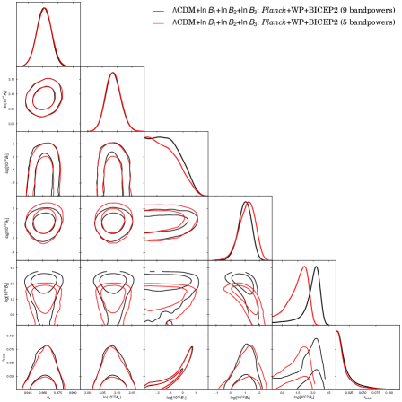
In this section we will start with the scalar spectrum reconstruction, and then turn to the tensor spectrum case. The prior ranges of the primordial spectrum parameters we studied are listed in Tab.1. Here we emphasize that the differences in the prior of tensor spectra amplitude at our cubic spline sampling knots when BICEP2 data are included, lie in the tension between Planck and BICEP2 data (we will show later). When our MCMC sampler investigates the wide parameter space spanned by (), at some points the resulting spectra are inconsistent with Planck TE cross-correlation data, in order to avoid this problem we have to adjust the prior ranges. But still the width of the priors are large enough and also the tensor amplitudes () get well constrained in these prior ranges as shown in Fig.9. So, we conclude that our prior choices will not affect the results significantly.
| Parameter | Range (min, max) |
|---|---|
III.1 Scalar spectrum reconstruction
Since the main capability of scalar spectrum reconstruction is driven by the CMB temperature data, we firstly study the case without BICEP2 polarization, i.e. only with Planck temperature and WMAP9 low- polarization (WP) data sets. As mentioned in the previous section, here we uniformly sample 3 points in the logarithmic scale of wavenumber, which are located at , and Mpc-1 with the logarithmic amplitudes , and , respectively. And then, we sample the parameter space spanned by vanilla CDM parameters without the scalar amplitude and its index tilt and replacing them with , and , hereafter we call this parameter compilation as CDM--+++.
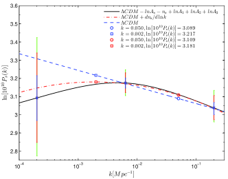
The marginalized mean scalar spectrum reconstructed from Planck+WP data is represented by the black solid curve in Fig. 1 and the corresponding error bars at the sampling points are denoted by the blue, red and green segments, respectively. For comparison, we also show the primordial scalar spectrum from the Planck marginalized mean vanilla CDM and CDM+ (scalar index running) with blue dashed and red dotted-dashed curves. From Fig. 1, we can see that, first, our cubic spline interpolation result mimics the CDM+ case; second, on Mpc-1 scale, the simplest vanilla model is disfavored at nearly level.
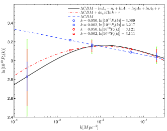
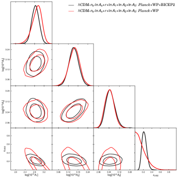
Adding the BICEP2 polarization data, we show the results in Fig. 2 for models including the tensor-to-scalar ratio , i.e. CDM--++++. We find that, first of all, due to the anti-correlation between scalar and tensor amplitudes (see the bottom left sub-panel of Fig. 8 in Appendix A), the large value of tensor-to-scalar ratio discovered by BICEP2 data will lead to the suppression of scalar amplitude on the large scales. This is also explicitly demonstrated in the top sub-panel of Fig. 8 in Appendix A. As a result of deficit of scalar power on the large scales, as shown in Fig. 2 the vanilla CDM model (blue curve) is strongly disfavored with confidence level on the Mpc-1 scale. A similar result is obtained by authors of Abazajian:2014tqa . By using Planck and BICEP2 data, they found a distinct preference for a suppression of power in the scalar spectrum at large scales, Mpc-1 via a linear spline reconstruction method. Second, by assuming the scale invariant tensor spectrum, our scalar spectrum cubic spline interpolation parameterization still gives a large tensor-to-scalar ratio at C.L., see Tab. 2 in Appendix A.
III.2 Tensor spectrum reconstruction
In the previous subsection, we have assumed the tensor spectrum is scale-invariant. In this subsection we relax the assumption and use the same cubic spline interpolation method to reconstruct the shape of tensor spectrum. Unlike the CMB temperature spectrum which is mainly sourced by the primordial scalar perturbations, the B-mode polarization anisotropy seeded by tensor perturbation is only detected by BICEP2 on the large scales with the polar spherical harmonic mulitpoles ranged (9 bandpowers). As the case for the scalar spectrum, here the tensor spectrum is also uniformly sampled with 3 points in the logarithmic scale of wavenumber, but only on the scales covered by BICEP2 observations. Consequently, we sample them at , and Mpc-1, respectively. The cosmological parameters we estimated are the 6 vanilla CDM model parameters plus the extra 3 tensor amplitudes , and .
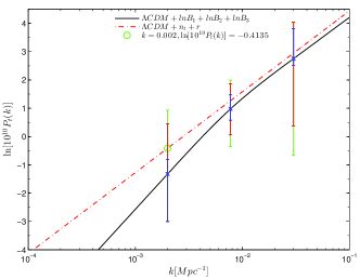
In Fig. 3 we plot the primordial tensor spectra from the best-fit model of CDM+++ (black solid curve) and CDM++ (red dotted-dashed curve) as well as the error bars at the sampling points of the cubic spline interpolation method. First of all, both the standard power-law and our cubic spline parameterizations favor a blue-tilt tensor spectrum. The former (see Tab.3 in AppendixB) reports
| (6) | |||||
| (7) |
and our cubic spline interpolation method gives
| (8) |
Second, we notice that in our cubic spline interpolation method the slope of the tensor spectrum becomes larger in the low- regime, but still is consistent with the power-law parameterization in confidence level.
As we argued in the previous section, there exists an extraordinary power excess in the higher wavenumber regimes of BICEP2 data. Given this consideration, in what follows we only adopt the selected first 5 bandpower data of BICEP2 for our reconstruction. Based on the multipole ranges covered by these powerbands (), we sample points at , and Mpc-1, respectively.
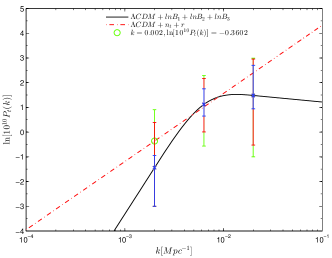
The reconstructed tensor spectra as well as error bars are shown in Fig. 4. First, from the power-law parameterization, we can see that the blue tensor spectra are still favored but with the tilt becomes smaller as expected
| (9) | |||||
| (10) |
Second, with only the first 5 bandpower data, unlike the simplest power-law parameterization, a non-trivial shape of tensor spectrum is obtained. Concretely, in the range of BICEP2 data favor a large tensor blue-tilt, while when Mpc-1 the spectrum becomes almost flat. This is due to the fact that we do not use the last 4 bandpower data. The resulting tensor-to-scalar ratio in our cubic spline interpolation method is
| (11) |
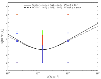
Because the above blue tensor tilt is significantly inconsistent with the standard inflationary prediction, we have to figure out its reason on the data analysis level. Notice that for now we always utilize Planck+WP+BICEP2 data compilation, so one natural guess is that this blue tensor tilt might reflect the tension among Planck, WMAP polarization and BICEP2 data sets. In order to justify our conjecture, we have to remove the above data sets one by one. Since we vary both the primordial spectrum and standard CDM parameters, such as baryon (), cold dark matter density () etc, we have to keep the robust Planck temperature data in order to get well estimations of the CDM parameters. Hence, we first remove the BICEP2, i.e. using Planck+WP, and further discard WMAP polarization data, i.e. only using Planck temperature data. However, due to the fact that CMB temperature data are insensitive to the reionization optical depth (), if we discard WMAP polarization data we have to include gaussian prior on to break the well-known degeneracy between and the scalar amplitude . Here we take the gaussian prior as
| (12) |
Besides this, because the contribution of tensor spectra to CMB temperature anisotropies is only significant in the mulitpole range (), when we use Planck+WP or Planck+ prior data sets, we sample the knots of tensor spectra in the range of .
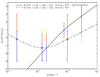
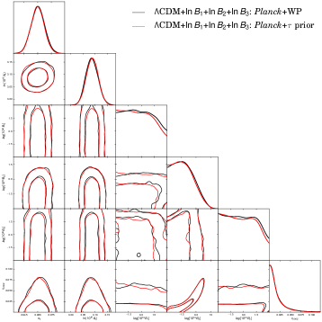
The resulting primordial tensor spectrum shape, corresponding marginalized 1D/2D posterior distributions and parameter regimes are shown in Fig.5, Fig.10 and Tab.5. First, we can see that the reconstructed tensor spectra from Planck+WP and Planck+ prior are very similar, both the central values and the marginalized error bars. So, we can draw the conclusion that WMAP low- polarization data are not crucial for the tensor reconstruction results. Second, as shown in Fig.6 the error bars from Planck temperature data are quite large compared with those from the data compilation Planck+WP+BICEP2 (see the error bars at sampling knot Mpc-1 in the dashed black curve and those at the second knot in the black solid curve in Fig.6). It means that the current Planck temperature data are not rubost to determine the shape of the primordial tensor spectrum. The resulting tensor spectrum from only Planck temperature data could be any shape among red, blue or scale-invariant types. Third, when we compare the second knot in Planck+WP (dashed black curve) and the first left knot Planck+WP+BICEP2 results (solid black curve), Fig.6 shows that both their central value and marginalized error bars are very close. It reflects the fact that the reconstructed tensor spectrum in the low- regime is actually driven by Planck temperature data. Furthermore, considering the fact that the BICEP2 data dominate the high- part, we conclude that our reconstructed blue tensor tilt are due to the tension between Planck and BICEP2 data sets, i.e. the fact that small tensor amplitude signals from Planck temperature data dominates the large scale reconstruction, while the large tensor amplitude signals from BICEP2 B-mode polarization data dominates the small scale reconstruction, leads to the resulting blue tensor tilt.
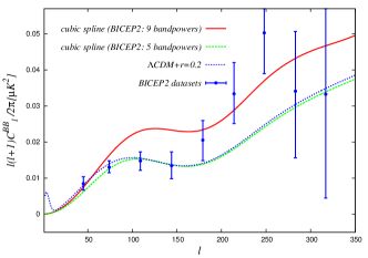
Finally, in order to give an intuitive impression of our reconstruction result, in Fig. 7 we plot the BB auto-correlation power spectrum of our marginalized mean models (listed in Tab. 4 of Appendix B) as well as the scale-invariant tensor spectrum with model against the BICEP2 bandpowers data sets. We can see that in order to fit the BICEP2 data in the last 4 bandpowers, compared with the 5 bandpower reconstruction result (green curve) and the scale-invariant one (blue), the 9 bandpower (red) curve grows up in the high- regime significantly.
IV Conclusions
Starting with a purely phenomenological point of view, in this paper we have reconstructed the shape of the primordial scalar and tensor spectra by using the cubic spline interpolation method with Planck temperature and BICEP2 B-mode polarization data sets. We find that, due to the anti-correlation between scalar and tensor amplitudes on the large scales, the large value of tensor-to-scalar ratio discovered by BICEP2 data will lead to the suppression of scalar amplitude in this regime. Concretely, the vanishing scalar index running model is strongly disfavored by Planck+WP+BICEP2 data compilation with more than confidence level on the Mpc-1 scale. Furthermore, for the tensor spectrum reconstruction, a blue-tilt spectrum is obtained no matter using only the first 5 bandpowers or the full 9 bandpowers of BICEP2 data sets. Because of the large tensor tilt, compared with the large tensor-to-scalar ratio value () under the scale-invariant assumption, our cubic spline interpolation method gives and by using the data sets Planck+WP+BICEP2 (5 bandpowers) and (9 bandpowers), respectively. Finally, we also studied the data without BICEP2, we found that our resulting blue tensor tilt actually reflects the tension in the tensor amplitude between Planck (small amplitude but dominate the reconstruction on the large scale) and BICEP2 (large amplitude but dominate the reconstruction on the small scale) data sets.
Our results show that the conclusion of the blue-tilt tensor spectrum is very significant and independent of using power-law or cubic spline parameterizations. More important, this blue-tilt spectrum is not consistent with the prediction of the standard single field inflationary paradigm . On the one hand, it asks for a more careful cross-check with future experiments, such as the polarization data of Planck and Keck Array. On the other hand, once this discovery is confirmed, it will lead to a paradigm revolution about our understanding of the early universe.
Acknowledgements.
BH are indebted to Ana Achúcarro, Sabino Matarrese, Nicola Bartolo, Wessel Valkenburg and Frederico Arroja for various helpful discussions. BH is supported by the Dutch Foundation for Fundamental Research on Matter (FOM). JWH, ZKG and RGC are partially supported by the project of Knowledge Innovation Program of Chinese Academy of Science, NSFC under Grant No.11175225, No.11335012, and National Basic Research Program of China under Grant No.2010CB832805 and No.2010CB833004.Appendix A Marginalized statistics in scalar spectrum reconstruction
Here we list the various marginalized statistical results for cubic spline interpolation and power-law parameterizations of scalar spectrum, including 1D, 2D marginalized posterior distribution, marginalized mean values as well as the (or ) confidence levels.
| CDM--++++ | CDM++ | ||
|---|---|---|---|
| Planck+WP | Planck+WP+BICEP2 (9 bandpowers) | Planck+WP+BICEP2 (9 bandpowers) | |
| Parameters | mean C.L. | mean C.L. | mean C.L. |
| 2.2240.031 | 2.2240.030 | 2.2380.028 | |
| 0.12040.0028 | 0.12020.0027 | 0.11860.0017 | |
| 1.041250.00065 | 1.041330.00063 | 1.041500.00057 | |
| 0.1030.016 | 0.1060.017 | 0.1050.016 | |
| 3.1220.033 | |||
| 0.96000.0063 | |||
| (CL) | |||
| (CL) | (CL) | (CL) | |
| 2.890.20 | 2.830.15 | ||
| 3.1570.032 | 3.1540.029 | ||
| 3.0450.034 | 3.0500.034 | ||
| 0.3180.018 | 0.3160.017 | 0.3060.010 | |
| 67.221.27 | 67.341.22 | 68.060.79 | |
| 4901.833 | 4921.868 | 4924.052 | |
Appendix B Marginalized statistics in tensor spectrum reconstruction
Here we list the various marginalized statistical results for cubic spline interpolation and power-law parameterizations of tensor spectrum, including 1D, 2D marginalized posterior distribution, marginalized mean values as well as the (or ) confidence levels.
| CDM++ | ||
|---|---|---|
| Planck+WP+BICEP2 (9 bandpowers) | Planck+WP+BICEP2 (5 bandpowers) | |
| Parameters | mean C.L. | mean C.L. |
| 2.2000.028 | 2.2040.028 | |
| 0.11940.0026 | 0.11950.0027 | |
| 1.041290.00064 | 1.041270.00063 | |
| 0.0900.013 | 0.0890.013 | |
| 0.96110.0073 | 0.96150.0073 | |
| 3.0870.025 | 3.0860.025 | |
| (CL) | (CL) | |
| (CL) | (CL) | |
| 0.3130.016 | 0.3130.016 | |
| 67.381.19 | 67.401.11 | |
| (CL) | (CL) | |
| 4920.773 | 4909.861 | |
| CDM+++ | ||
|---|---|---|
| Planck+WP+BICEP2 (9 bandpowers) | Planck+WP+BICEP2 (5 bandpowers) | |
| Parameters | mean C.L. | mean C.L. |
| 2.2020.028 | 2.2020.028 | |
| 0.11940.0026 | 0.11950.0026 | |
| 1.041300.00063 | 1.041250.00062 | |
| 0.0900.013 | 0.0900.013 | |
| 0.96100.0071 | 0.96140.0072 | |
| 3.0870.025 | 3.0870.025 | |
| (CL) | (CL) | |
| (CL) | (CL) | |
| (CL) | (CL) | |
| 0.3130.016 | 0.3140.016 | |
| 67.431.17 | 67.371.17 | |
| (CL) | (CL) | |
| 4920.558 | 4909.799 | |
| CDM+++ | ||
|---|---|---|
| Planck+WP | Planck+ Prior | |
| Parameters | mean C.L. | mean C.L. |
| 2.2040.028 | 2.2030.028 | |
| 0.12000.0028 | 0.12010.0027 | |
| 1.041220.00063 | 1.041190.00063 | |
| 0.0890.013 | 0.0900.012 | |
| 0.96030.0074 | 0.95990.0071 | |
| 3.0870.025 | 3.0890.024 | |
| (CL) | (CL) | |
| (CL) | (CL) | |
| (CL) | (CL) | |
| 0.3170.017 | 0.3170.016 | |
| 67.201.22 | 67.141.17 | |
| (CL) | (CL) | |
| 4902.387 | 3895.305 | |
References
- (1) P. A. R. Ade et al. [BICEP2 Collaboration], arXiv:1403.3985 [astro-ph.CO].
- (2) P. A. R. Ade et al. [Planck Collaboration], arXiv:1303.5082 [astro-ph.CO].
- (3) W. Hu and M. J. White, Phys. Rev. D 56, 596 (1997) [astro-ph/9702170].
- (4) K. M. Smith, C. Dvorkin, L. Boyle, N. Turok, M. Halpern, G. Hinshaw and B. Gold, arXiv:1404.0373 [astro-ph.CO].
- (5) G. Hinshaw et al. [WMAP Collaboration], Astrophys. J. Suppl. 208, 19 (2013) [arXiv:1212.5226 [astro-ph.CO]].
- (6) S. Das, T. Louis, M. R. Nolta, G. E. Addison, E. S. Battistelli, J R. Bond, E. Calabrese and D. C. M. J. Devlin et al., arXiv:1301.1037 [astro-ph.CO].
- (7) R. Keisler, C. L. Reichardt, K. A. Aird, B. A. Benson, L. E. Bleem, J. E. Carlstrom, C. L. Chang and H. M. Cho et al., Astrophys. J. 743, 28 (2011) [arXiv:1105.3182 [astro-ph.CO]].
- (8) K. T. Story, C. L. Reichardt, Z. Hou, R. Keisler, K. A. Aird, B. A. Benson, L. E. Bleem and J. E. Carlstrom et al., Astrophys. J. 779, 86 (2013) [arXiv:1210.7231 [astro-ph.CO]].
- (9) C. L. Reichardt, L. Shaw, O. Zahn, K. A. Aird, B. A. Benson, L. E. Bleem, J. E. Carlstrom and C. L. Chang et al., Astrophys. J. 755, 70 (2012) [arXiv:1111.0932 [astro-ph.CO]].
- (10) V. íc. Miranda, W. Hu and P. Adshead, arXiv:1403.5231 [astro-ph.CO].
- (11) D. K. Hazra, A. Shafieloo, G. F. Smoot and A. A. Starobinsky, arXiv:1403.7786 [astro-ph.CO].
- (12) R. Bousso, D. Harlow and L. Senatore, arXiv:1404.2278 [astro-ph.CO].
- (13) D. K. Hazra, A. Shafieloo and G. F. Smoot, arXiv:1404.0360 [astro-ph.CO].
- (14) M. Kawasaki and S. Yokoyama, arXiv:1403.5823 [astro-ph.CO].
- (15) M. Kawasaki, T. Sekiguchi, T. Takahashi and S. Yokoyama, arXiv:1404.2175 [astro-ph.CO].
- (16) E. Giusarma, E. Di Valentino, M. Lattanzi, A. Melchiorri and O. Mena, arXiv:1403.4852 [astro-ph.CO].
- (17) J. -F. Zhang, Y. -H. Li and X. Zhang, arXiv:1403.7028 [astro-ph.CO].
- (18) C. Dvorkin, M. Wyman, D. H. Rudd and W. Hu, arXiv:1403.8049 [astro-ph.CO].
- (19) C. R. Contaldi, M. Peloso and L. Sorbo, arXiv:1403.4596 [astro-ph.CO].
- (20) B. Freivogel, M. Kleban, M. R. Martinez and L. Susskind, arXiv:1404.2274 [astro-ph.CO].
- (21) H. Firouzjahi and M. H. Namjoo, arXiv:1404.2589 [astro-ph.CO].
- (22) Y. -F. Cai, J. -O. Gong and S. Pi, arXiv:1404.2560 [hep-th].
- (23) C. Cheng, Q. -G. Huang and W. Zhao, arXiv:1404.3467 [astro-ph.CO].
- (24) S. Choudhury and A. Mazumdar, arXiv:1403.5549 [hep-th].
- (25) S. Hotchkiss, A. Mazumdar and S. Nadathur, JCAP 1202, 008 (2012) [arXiv:1110.5389 [astro-ph.CO]].
- (26) M. Gerbino, A. Marchini, L. Pagano, L. Salvati, E. Di Valentino and A. Melchiorri, arXiv:1403.5732 [astro-ph.CO].
- (27) F. Wu, Y. Li, Y. Lu and X. Chen, arXiv:1403.6462 [astro-ph.CO].
- (28) C. Cheng and Q. -G. Huang, arXiv:1403.7173 [astro-ph.CO].
- (29) H. Li, J. -Q. Xia and X. Zhang, arXiv:1404.0238 [astro-ph.CO].
- (30) B. Chang and L. Xu, arXiv:1404.1558 [astro-ph.CO].
- (31) M. Baldi, F. Finelli and S. Matarrese, Phys. Rev. D 72, 083504 (2005) [astro-ph/0505552].
- (32) Y. -S. Piao and Y. -Z. Zhang, Phys. Rev. D 70, 063513 (2004) [astro-ph/0401231].
- (33) T. Kobayashi, M. Yamaguchi and J. ’i. Yokoyama, Phys. Rev. Lett. 105, 231302 (2010) [arXiv:1008.0603 [hep-th]].
- (34) R. H. Brandenberger, A. Nayeri and S. P. Patil, arXiv:1403.4927 [astro-ph.CO].
- (35) P. Creminelli, M. A. Luty, A. Nicolis and L. Senatore, JHEP 0612, 080 (2006) [hep-th/0606090].
- (36) P. Creminelli and L. Senatore, JCAP 0711, 010 (2007) [hep-th/0702165].
- (37) E. I. Buchbinder, J. Khoury and B. A. Ovrut, Phys. Rev. D 76, 123503 (2007) [hep-th/0702154].
- (38) J. -Q. Xia, Y. -F. Cai, H. Li and X. Zhang, arXiv:1403.7623 [astro-ph.CO].
- (39) T. Qiu, arXiv:1404.3060 [gr-qc].
- (40) Y. -S. Piao, B. Feng and X. -m. Zhang, Phys. Rev. D 69, 103520 (2004) [hep-th/0310206].
- (41) Z. -G. Liu, Z. -K. Guo and Y. -S. Piao, Phys. Rev. D 88, 063539 (2013) [arXiv:1304.6527 [astro-ph.CO]].
- (42) J. -O. Gong, arXiv:1403.5163 [astro-ph.CO].
- (43) Y. Wang and W. Xue, arXiv:1403.5817 [astro-ph.CO].
- (44) C. Sealfon, L. Verde and R. Jimenez, Phys. Rev. D 72, 103520 (2005) [astro-ph/0506707].
- (45) L. Verde and H. V. Peiris, JCAP 0807, 009 (2008) [arXiv:0802.1219 [astro-ph]].
- (46) H. V. Peiris and L. Verde, Phys. Rev. D 81, 021302 (2010) [arXiv:0912.0268 [astro-ph.CO]].
- (47) Z. -K. Guo, D. J. Schwarz and Y. -Z. Zhang, JCAP 1108, 031 (2011) [arXiv:1105.5916 [astro-ph.CO]].
- (48) Z. -K. Guo and Y. -Z. Zhang, JCAP 1111, 032 (2011) [arXiv:1109.0067 [astro-ph.CO]].
- (49) Z. -K. Guo and Y. -Z. Zhang, Phys. Rev. D 85, 103519 (2012) [arXiv:1201.1538 [astro-ph.CO]].
- (50) G. Aslanyan, L. C. Price, K. N. Abazajian and R. Easther, arXiv:1403.5849 [astro-ph.CO].
- (51) K. N. Abazajian, G. Aslanyan, R. Easther and L. C. Price, arXiv:1403.5922 [astro-ph.CO].
- (52) J. A. Vazquez, M. Bridges, M. P. Hobson and A. N. Lasenby, JCAP 1206, 006 (2012) [arXiv:1203.1252 [astro-ph.CO]].
- (53) J. A. Vazquez, M. Bridges, Y. -Z. Ma and M. P. Hobson, JCAP 1308, 001 (2013) [arXiv:1303.4014 [astro-ph.CO]].
- (54) P. A. R. Ade et al. [Planck Collaboration], arXiv:1303.5075 [astro-ph.CO].
- (55) P. A. R. Ade et al. [Planck Collaboration], arXiv:1303.5076 [astro-ph.CO].
- (56) A. Lewis, A. Challinor and A. Lasenby, Astrophys. J. 538, 473 (2000) [astro-ph/9911177].
- (57) A. Lewis and S. Bridle, Phys. Rev. D 66, 103511 (2002) [astro-ph/0205436].