Parametrizing the transition to the phantom epoch with Supernovae Ia and Standard Rulers

Abstract

The reconstruction of a (non)canonical scalar field Lagrangian from the dark energy Equation of State (EoS) parameter is studied, where it is shown that any EoS parametrization can be well reconstructed in terms of scalar fields. Several examples of EoS parameters are studied and the particular scalar field Lagrangian is reconstructed. Then, we propose some new parametrizations that may present a (fast) transition to a phantom dark energy EoS (where $w_{DE}<-1$) and the scalar field Lagrangian is also reconstructed numerically. Furthermore, the properties of these parametrizations of the dark energy EoS are studied by using supernovae Ia data (HST Cluster Supernova Survey) combined with Standard Ruler datasets [Cosmic Microwave Background (CMB) and Baryon Acoustic Oscillations (BAO)] and its comparison with the $\Lambda$CDM model is analyzed. Then, the best fit of the models is obtained, which provides some information about whether a phantom transition may be supported by the observations. In this regard, the crossing of the phantom barrier is allowed statistically but the occurrence of a future singularity seems unlikely.

I Introduction

In 1998 a deviation on the luminosity distance of Supernovae Ia (Sne Ia) was observed by two independent groups SN1 , a fact that was interpreted as the acceleration of the universe expansion. Later on, other independent observations such as the Cosmic Microwave Background (CMB) WMAP -Ade:2013zuv or the Baryon Acoustic Oscillations (BAO) Eisenstein:2005su have confirmed such hypothesis, which has been widely accepted by the scientific community since then. Then, a large number of candidates, enclosed under the name of dark energy, have been proposed in order to understand the mechanism that produces such accelerating expansion (for a review on dark energy candidates see R-DE ). The list of models includes a cosmological constant, canonical/phantom scalar fields Quintessence , vector fields VT or modifications of General Relativity (GR) modified-gravity , among others.

Moreover, an interesting and useful approach for analyzing dark energy models is aimed to study the dark energy equation of state (EoS) as an effective description instead of reconstructing theoretical models. In this sense, dynamical EoS’s that deviate from the cosmological constant have been widely studied, where perfect fluids with inhomogeneous EoS and redshift-dependent parameters have been proposed which may accomplish the late-time acceleration, and even the entire cosmological history by unifying the dark energy epoch and the inflationary phase (see Ref. Nojiri:2005sr ). Moreover, an effective description of the behavior of the dark energy EoS simplifies the fit of the free parameters while comparing with observational data, such that theoretical models, as modified gravities or scalar-tensor theories, can be tested by using effective parametrizations of the EoS along the period of interest of the universe evolution. In this regard, several parametrizations of the dark energy EoS have been proposed over the last decade and its comparison with observational data has been studied (see Refs. Huterer:2000mj -Lazkoz:2007cc ). Some of these models lead to $\Lambda$CDM as the one with major statistical support but also other possibilities are allowed. Furthermore, the possibility that dark energy behaves as a phantom fluid, whose effective EoS parameter would turn out $w_{DE}<-1$, has been also widely explored in the literature (see Ref. phantom ) in spite of that such transition may lead to large instabilities in some particular phantom models vikman . Such kind of EoS produces a phase of super-accelerating expansion that may end in a future singularity (for a classification of future singularities, see Refs. Nojiri:2005sx -barrow1 ), whose analysis has attracted much interest, as may content important information on the structure of spacetime and its topology (see Ref. barrow ). Hence, singular cosmologies have been explored within several frameworks, including modified gravities (see Ref. Nojiri:2008fk ). Furthermore, observations seem not to discard every phantom scenario and even some analysis highly support such possibility when studying carefully the observational data Lazkoz:2006gp .

In the present paper, we present a reconstruction method for the action of a (non)canonical scalar field by just specifying the EoS parameter. Then, some examples of parametrizations of the dark energy EoS are reconstructed in terms of the scalar field. Such reconstruction method may be extended to other theoretical models as modified gravities to obtain the gravitational action from the dark energy EoS. The aim of such reconstruction is to provide a method to relate a phenomenological description, as the dark energy EoS, with the underlying theory that leads to such phenomenological behavior. Then, we propose some new EoS parametrizations that experience fast changes, and which may give rise to fast crossings of the phantom barrier and eventually to the occurrence of a future singularity. The best fit of the free parameters of the models are found by using some observational datasets from Standard rulers (CMB Spergel:2006hy and BAO Eisenstein:2005su ) and Sne Ia Suzuki:2011hu . The comparison of the results obtained by using each dataset is analyzed as well as the comparison with the $\Lambda$CDM model. The value of the relative matter density $\Omega_{m}^{0}$ is found to be very close to the $\Lambda$CDM model, while the best fit of the EoS parameters does not discard the transition to the phantom epoch but disfavor the occurrence of future singularities.

The paper is organized as follows: section II deals with the reconstruction of scalar field models from the dark energy EoS. Then, section III is devoted to the analysis of some new parametrizations of the EoS, where a preliminary study of the cosmological evolution and the occurrence of future singularities are analyzed. Section IV deals with the fit of the free parameters of the model with observational data and its comparison with $\Lambda$CDM. Finally, in section V, we discuss the results of the paper.

II Reconstructing scalar field models from the dark energy EoS

Let us consider a simple model with a scalar field besides the matter content. Such an action can be expressed as follows Quintessence

$$S=\int dx^{4}\sqrt{-g}\left[\frac{1}{2\kappa^{2}}R-\frac{1}{2}\gamma(\phi)\partial_{\mu}\phi\partial^{\mu}\phi-V(\phi)+\mathcal{L}_{m}\right]\ ,$$ (1)

where $\kappa^{2}=8\pi G$, $\mathcal{L}_{m}$ is the matter Lagrangian density whereas $\gamma(\phi)$ and $V(\phi)$ represent the kinetic term and the potential of the scalar field $\phi$ respectively. By assuming a spatially flat Friedmann-Lemaître-Robertson-Walker (FLRW) metric $ds^{2}=-dt^{2}+a^{2}(t)\sum_{i=1}^{3}dx_{i}^{2}$, the resulting equations are given by

$$H^{2}=\left(\frac{\dot{a}}{a}\right)^{2}=\frac{\kappa^{2}}{3}\left(\rho_{m}+\rho_{\phi}\right)\ ,\quad\quad\dot{H}=-\frac{\kappa^{2}}{2}\left(\rho_{m}+p_{m}+\rho_{\phi}+p_{\phi}\right)\ ,$$ (2)

where

$$\rho_{\phi}=\frac{1}{2}\gamma(\phi)\,{\dot{\phi}}^{2}+V(\phi)\ ,\quad\quad p_{\phi}=\frac{1}{2}\gamma(\phi)\,{\dot{\phi}}^{2}-V(\phi)\ ,$$ (3)

while the scalar field equation yields,

$$\ddot{\phi}+3H\dot{\phi}+\frac{1}{2\gamma(\phi)}\left[\gamma^{\prime}(\phi)\dot{\phi}^{2}+2V^{\prime}(\phi)\right]=0\ .$$ (4)

The matter content is described by a perfect fluid with a constant EoS $p_{m}=w_{m}\rho_{m}$, such that the continuity equation $\dot{\rho}_{m}+3H(1+w_{m})\rho_{m}=0$ can be easily solved leading to

$$\rho_{m}=\rho_{0}a^{-3(1+w_{m})}=\rho_{0}(1+z)^{3(1+w_{m})}\ ,$$ (5)

where $1+z=1/a$ is the redshift and $a_{0}=1$ is the value of the scale factor evaluated today. Furthermore, the EoS parameter for the scalar field $\phi$ is defined as follows

$$w_{\phi}=\frac{p_{\phi}}{\rho_{\phi}}=-1+\frac{\gamma(\phi)\dot{\phi}^{2}}{\frac{1}{2}\gamma(\phi)\dot{\phi}^{2}+V(\phi)}\ ,$$ (6)

where $w_{\phi}$ depends in general on the cosmic time, or equivalently on the redshift. Note that any phantom transition gives rise to change the sign of the kinetic term $\gamma(\phi)$ as $\rho_{\phi}$ is defined positive. In addition, the assumption of the kinetic factor $\gamma(\phi)$ allows to redefine the scalar field, so that the scalar Lagrangian density can be easily reconstructed, as shown below. Then, introducing (5-6) in the FLRW equations (2) and rewriting the equations in terms of the redshift instead of the cosmic time, the equation for the Hubble parameter reduces to

$$2H(1+z)H^{\prime}-3H^{2}(1+w_{\phi}(z))+3H^{2}_{0}\Omega_{m}^{0}(1+z)^{3(1+w_{m})}w_{\phi}(z)=0\ ,$$ (7)

where $\Omega_{m}^{0}=\frac{\rho_{m0}}{3H_{0}^{2}/\kappa^{2}}$ is the relative matter density and $H_{0}$ is the experimental value of the Hubble parameter evaluated today ($z=0$). In order to simplify the equation (7) the Hubble parameter can be redefined as $H(z)=H_{0}\ E(z)$. Then, the equation (7) becomes

$$2E(z)(1+z)E^{\prime}(z)-3E^{2}(z)(1+w_{\phi}(z))+3\Omega_{m}^{0}(1+z)^{3(1+w_{m})}w_{\phi}(z)=0\ .$$ (8)

Hence, by specifying the EoS parameter (6), the Hubble evolution $E(z)$ is obtained by solving the equation (8). Note that in the case $w_{\phi}=-1$, the kinetic term becomes null $\gamma(\phi)=0$ and the scalar field turns out constant, such that the action is reduced to the $\Lambda$CDM model with a cosmological constant given by $2\Lambda=V_{0}$. Let us now consider the dynamical case, where the EoS parameter (6) evolves with time. In such a case the following scalar potential and kinetic term are assumed,

$$\gamma(\phi) = -\frac{2}{\kappa^{2}}\frac{g^{\prime}(\phi)}{\phi g(\phi)}-\frac{1+w_{m}}{g^{2}}\rho_{m0}\phi^{-(5+3w_{m})}\ ,$$

$$V(\phi) = -\left(\frac{1-w_{\phi}(\phi)}{2(w_{\phi}(\phi)+1)}\right)\left(\frac{2}{\kappa^{2}}\phi g^{\prime}(\phi)g(\phi)+\rho_{m0}(1+w_{m})\phi^{-3(1+w_{m})}\right)\ ,$$ (9)

which lead to the general solution,

$$H=g\left(\frac{1}{1+z}\right)\ \quad\text{and}\quad\phi=\frac{1}{1+z}\ .$$ (10)

Let us illustrate the above reconstruction by considering some examples. Firstly, the well known parametrization of the dark energy EoS suggested in Huterer:2000mj , which is given by

$$w(z)=w_{0}+w_{1}z,\quad w_{1}=\left(\frac{dw}{dz}\right)_{z=0}\ .$$ (11)

This parametrization, also called Linear Redshift Parametrization, initially proposed by Huterer and Turner in 2001 and by Weller and Albrecht in 2002, is only compatible with low redshift data ($z<1$) since grows linearly in redshift. In this case, the equation (8) can be solved exactly by considering a pressureless matter fluid $w_{m}=0$, and it yields

$$H(z)=H_{0}\left(1+z\right)^{\frac{3}{2}(1-w_{1})}\sqrt{\Omega_{m}^{0}(1+z)^{3w_{1}}+C_{1}{\rm e}^{3w_{1}(1+z)}(1+z)^{3w_{0}}}\ ,$$ (12)

where $C_{1}$ is an integration constant. Then, the kinetic term and the scalar potential (9) can be obtained, where $g(\phi)=H(\frac{1-\phi}{\phi})$ given by (12),

$$\gamma(\phi)=\frac{3C_{1}}{\kappa^{2}}\frac{w_{1}\left(1-\phi\right)+(1+w_{0})\phi}{C_{1}{\rm e}^{\frac{3w_{1}}{\phi}}\phi^{3}+\Omega_{m}\phi^{3(1+w_{0}-w_{1})}}{\rm e}^{\frac{3w_{1}}{\phi}}\ ,$$

$$V(\phi)=\frac{3C_{1}H_{0}^{2}}{2\kappa^{2}}\left[w_{1}(-1+\phi)+(1-w_{0})\phi\right]{\rm e}^{\frac{3w_{1}}{\phi}}\phi^{-4+3(w_{1}-w_{0})}\ .$$ (13)

Hence the scalar field Lagrangian (1) is fully reconstructed. Moreover, the best fit of the EoS parameters (11) when set with SNe Ia data are given by $w_{0}=-1.4$ and $w_{1}=1.67$, Dicus:2004cp , which presents a phantom transition which is well described by the kinetic term and scalar potential (13), where $\gamma(\phi)$ changes its sign along the universe evolution. Let us consider now a slightly modified parametrization,

$$w(z)=w_{0}+w_{1}z+w_{2}z^{2}\ ,$$ (14)

where a second order correction is included. Then, by solving the FLRW equations (8), the Hubble parameter is given by

$$H(z)=H_{0}\left(1+z\right)^{\frac{3}{2}(1-w_{1})}\sqrt{\Omega_{m}^{0}(1+z)^{3w_{1}}+C_{1}{\rm e}^{\frac{3}{2}(1+z)[2w_{1}+w_{2}(z-3)]}(1+z)^{3(w_{0}+w_{2})}}\ ,$$ (15)

And then, the kinetic term and the scalar potential yield

$$\gamma(\phi)=\frac{3C_{1}}{\kappa^{2}}\frac{w_{2}\left(1-\phi\right)^{2}+\phi\left[w_{1}+\phi(1+w_{0}-w_{1})\right]}{C_{1}{\rm e}^{\frac{3(w_{2}+2w_{1}\phi)}{2\phi^{2}}}\phi^{4}+\phi^{3(1+w_{0}-w_{1})}}{\rm e}^{\frac{3(w_{2}+2w_{1}\phi)}{2\phi^{2}}}\ ,$$

$$V(\phi)=-\frac{3C_{1}H_{0}^{2}}{2\kappa^{2}}\left[w_{2}(-1+\phi)^{2}+w_{1}\phi+(-1+w_{0}-w_{1})\phi^{2}\right]{\rm e}^{\frac{3(w_{2}+(2w_{1}-4w_{2})\phi)}{2\phi^{2}}}\phi^{-4+3(w_{0}-w_{1}+w_{2})}\ .$$ (16)

Then, finally let us consider the following, also well known, parametrization Chevallier:2000qy ,

$$w(z)=w_{0}+w_{1}\frac{z}{1+z}\ .$$ (17)

Here the dark energy EoS tends to a constant for large redshifts while its dynamical behavior becomes important at small redshifts. Then, the Hubble parameter yields,

$$H(z)=H_{0}^{2}(1+z)^{3/2}\sqrt{\Omega_{m}+C_{1}(1+z)^{3(w_{0}+w_{1})}{\rm e}^{\frac{3w_{1}}{(1+z)}}}\ .$$ (18)

And as in the previous examples, the kinetic term and the scalar potential (9) which described the EoS parameter (17) are reconstructed leading to

$$\gamma(\phi)=\frac{3C_{1}}{\kappa^{2}}\frac{1+w_{0}+w_{1}(-1+\phi)}{C_{1}{\rm e}^{3w_{1}\phi}+\Omega_{m}\phi^{3(w_{0}+w_{1})}}{\rm e}^{3w_{1}\phi}\phi^{-2}\ ,$$

$$V(\phi)=\frac{3C_{1}H_{0}^{2}}{2\kappa^{2}}\left[1-w_{0}+w_{1}(-1+\phi)\right]{\rm e}^{3w_{1}\phi}\phi^{-3(1+w_{0}+w_{1})}\ .$$ (19)

Hence, the reconstruction method explained above provides a way to get the underlying scalar field action for a particular dark energy EoS. However, note that in general, more complex EoS parametrizations would not lead to exact expressions for scalar field Lagrangian, but numerical resources are required. In the next section, a new parametrization that also may transit to the phantom epoch is proposed and the best fit is found by using Sne Ia, CMB and BAO data. The reconstruction of the scalar field Lagrangian is analyzed by using numerical methods.

III Parametrizing the transition to the phantom epoch

Let us now assume a new parametrization for $w_{DE}(z)$ that may cross the phantom barrier ($w<-1$) along the universe evolution,

$$w_{1}(z)=-1+w_{0}\left[\tanh\left(z-z_{0}\right)-1\right]\ .$$ (20)

where $w_{0}$ and $z_{0}$ are free parameters. Specifically, $z_{0}$ displaces the turning point of the function along the $z$ axis and $w_{0}$ controls the value of the EoS parameter when $z\leq z_{0}$, and indeed how far the phantom barrier is crossed and the time for the occurrence of future singularities, as discussed below. Note also that for $w_{0}<0$, there will not be phantom epoch as $w_{1}>-1$ at any redshift.

Moreover, the above parametrization can be slightly modified to become a transition parametrization centered around $w=-1$, leading to the second parametrization that is analyzed here,

$$w_{2}(z)=-1+w_{0}\tanh\left(z-z_{0}\right)\ ,$$ (21)

where in this case $w_{0}$ controls the width of the strip around $w=-1$ in which the parametrization can evolve. Nevertheless, both parametrizations behaves as $\Lambda$CDM for $w_{0}=0$. Moreover, the EoS parameter (20) tends to $w_{1}\sim-1$ at large redshifts and the model (21) leads to $w_{2}\sim-1+w_{0}$, whereas $w_{1}=-1-w_{0}$ and $w_{2}=-1$ at $z=z_{0}$, the EoS transition point. Both parametrizations describe deviations from $\Lambda$CDM. Furthermore, the reconstruction of the scalar field Lagrangian studied in the previous section can be applied to both EoS but numerical resources have to be applied in order to obtain the kinetic term and the scalar potential, since the FLRW equation (7) does not lead to an exact solution in this case (see the Appendix for an exact solution using approximation methods). Then, for an illustrative purpose, the kinetic term and the scalar potential for a sample of the EoS models (20) and (21) are shown in Fig. 1. In both models, the scalar field rolls down along the potential at small redshifts when the dynamics of the scalar field becomes important, reaching a plato at the current time ($\phi=1$). The kinetic term presents also a similar asymptotic behavior. Consequently, both models tend to a constant EoS asymptotically.

(a)

(b)

Figure 1: Reconstruction of the kinetic term and the scalar potential for the parametrization $w_{1}$ (solid line) and $w_{2}$ (dashed line). Here we have assumed $w_{0}=-0.05$ and $z_{0}=12.14$ for the model (20) and $w_{0}=0.1$ and $z_{0}=-10$ for the model (21).

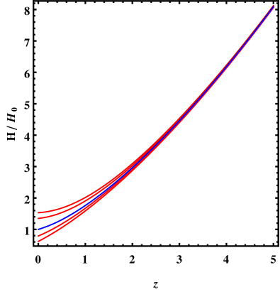
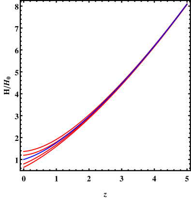
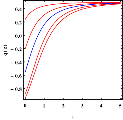
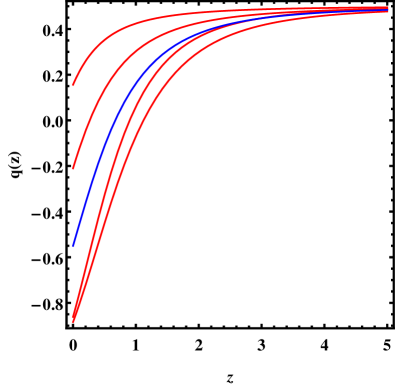
Let us now analyze the cosmological evolution in a qualitative way for both models (20) and (21). By assuming $\Omega_{m}^{0}=0.3$ and setting the initial conditions in order to fit $\Lambda$CDM at $z=2000$, the equation (8) is solved numerically for different values of the parameters $w_{0}$ and $z_{0}$, where we have assumed those values which approach closely to the $\Lambda$CDM model. Then, in Fig. 2, the evolution of the Hubble parameter is depicted, where the blue line corresponds to the $\Lambda$CDM model, whereas Fig. 3 shows the evolution of the deceleration parameter. At large redshifts, the functions match the $\Lambda$CDM model as expected, whereas at small redshifts, where the dynamical behavior of the EoS parameters (20) and (21) becomes important, both the Hubble parameter as the deceleration may provide differences with respect the $\Lambda$CDM model, as shown in Figs. 2-3.

(a)

(b)

Figure 2: Evolution of the Hubble parameter assuming the EoS parametrizations (20) and (21) in comparison with $\Lambda$CDM (blue line). For the first model (left panel), the parameter values are $(w_{0},z_{0})=\{(0.05,34.28),(0.05,12.14),(-0.05,12.14),(-0.1,34.28)\}$ from the upper to bottom. For the second model (right panel) the values in the same order are $(w_{0},z_{0})=\{(0.1,12.14),(0.15,12.14),(0.1,-10),(0.15,-10)\}$.

(a)

(b)

Figure 3: Evolution of the Hubble parameter for the EoS (20) and (21) in comparison with $\Lambda$CDM (blue line). For the first model (left panel), the parameter values are $(w_{0},z_{0})=\{(0.05,34.28),(0.05,12.14),(-0.05,12.14),(-0.1,34.28)\}$ from the bottom to upper. For the second model (right panel) the values in the same order are $(w_{0},z_{0})=\{(0.1,12.14),(0.15,12.14),(0.1,-10),(0.15,-10)\}$.

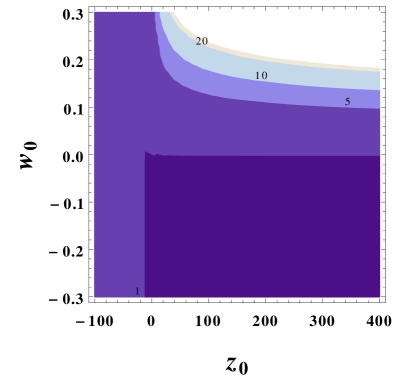
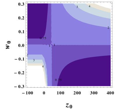
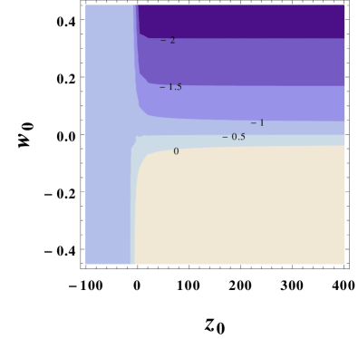
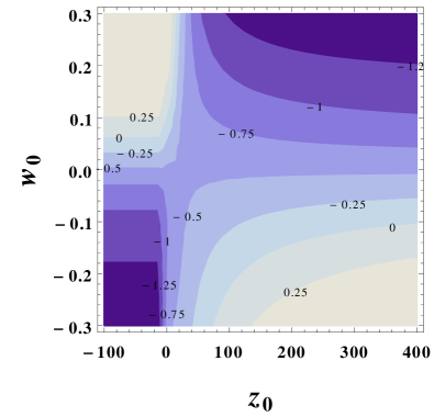
In order to analyze these differences with more accuracy, Figs. 4-5 show the values of $E(0)=H(0)/H_{0}$ and $q(0)$ evaluated today. Recalling that $E_{\Lambda CDM}(0)=1$ and $q_{\Lambda CDM}(0)=-0.5$ (with $\Omega_{m}^{0}=0.3$), the different predictions at $z=0$ can be easily compared.

(a)

(b)

Figure 4: Values of $E_{0}=H(0)/H_{0}$ as a function of the parameters $w_{0}$ and $z_{0}$ for the EoS parameters (20) and (21).

(a)

(b)

Figure 5: Values of $q_{0}$ as a function of the parameters $w_{0}$ and $z_{0}$ for the parametrizations (20) and (21).

Hence, the cosmological evolution is well reproduced by the EoS given in (20) and (21), where the free parameters can be restricted to avoid a large deviation from $\Lambda$CDM. However, note that the above models, and in general models with an EoS parameter $w<-1$ may imply the occurrence of future singularities. The study of future singularities has drawn much attention over the last years, mainly because of under certain conditions some realistic models with an appropriate cosmological evolution that satisfy the observational constraints, may give rise to some type of future singularity (see Ref. phantom ), but also because of theoretical implications since possible quantum effects close to the singularity become important. A classification of future singularities was proposed in Ref. Nojiri:2005sx ,

• Type I (“Big Rip”): For $t\rightarrow t_{s}$, $a\rightarrow\infty$ and $\rho\rightarrow\infty$, $|p|\rightarrow\infty$.

• Type II (“Sudden”): For $t\rightarrow t_{s}$, $a\rightarrow a_{s}$ and $\rho\rightarrow\rho_{s}$, $|p|\rightarrow\infty$ (see Ref. barrow1 ).

• Type III: For $t\rightarrow t_{s}$, $a\rightarrow a_{s}$ and $\rho\rightarrow\infty$, $|p|\rightarrow\infty$.

• Type IV: For $t\rightarrow t_{s}$, $a\rightarrow a_{s}$ and $\rho\rightarrow\rho_{s}$, $p\rightarrow p_{s}$ but higher derivatives of Hubble parameter diverge.

Nevertheless, the fact that the universe crosses the phantom barrier is not a sufficient condition for the occurrence of a future singularity, and may lead to other kind of non singular scenarios LittleRip . For a non constant EoS parameter $w$, the presence of future singularities depends on the asymptotic behavior of the EoS parameter. Then, by assuming a large value of the scale factor in comparison with the one today, $a\ggg 1$, when pressureless matter becomes negligible, the above models (20) and (21) can be approximated as follows

$$w_{1}(a)=-1+w_{0}\left[\tanh\left(\frac{1}{a}-1-z_{0}\right)-1\right]\sim-1-w_{0}\left[\tanh\left(1+z_{0}\right)+1\right]=\tilde{w_{1}}\ ,$$

$$w_{2}(a)=-1+w_{0}\tanh\left(\frac{1}{a}-1-z_{0}\right)\sim-1-w_{0}\tanh\left(1+z_{0}\right)=\tilde{w_{2}}\ .$$ (22)

Hence, the EoS parameters (20) and (21) become constant in the far future, whose value depends on the parameters $w_{0}$ and $z_{0}$. This coincides with the above analysis regarding the potential and the kinetic term of the scalar field that reproduces such models, where was found that the scalar field leads to a constant EoS asymptotically. Then, it is straightforward to solve the FLRW equations (2) which yield

$$H\sim\frac{2}{3|1+\tilde{w}|}\frac{1}{t_{s}-t}\ ,$$ (23)

where $1+\tilde{w}<0$ has been assumed and $t_{s}$ is the so called Rip time, the remained time for the occurrence of the Big Rip singularity. Hence, a future singularity will occur in case that $w_{0}>0$ in (20), whereas the expansion would evolute smoothly for $w_{0}<0$. Moreover, $\tilde{w}_{1}$ approaches $-1$ at low redshifts in case that $z_{0}$ takes negatives values independently of $w_{0}$ leading effectively to $\Lambda$CDM. In the second parametrization, the value of $\tilde{w}_{2}$ is greater than -1 for negative (positive) values of $w_{0}$ and $z_{0}>-1$ ($z_{0}<-1$), so there is no singularity. For positive (negative) values of $w_{0}$ and $z_{0}>-1$ ($z_{0}<-1$), the value of $\tilde{w}_{2}$ is below $-1$ and a singularity emerges, whereas $\tilde{w}_{2}$ tends asymptotically to $-1$ for $w_{0}=0$ and/or $z_{0}=-1$.

Thus, depending on the free parameters, the above models may lead to some kind of future singularity.

IV Fitting the models with SNe Ia data and standard rulers

Firstly we compute the best fit for the above parametrizations by using the SNe dataset of $557$ SN stars of union2 (see Ref. Suzuki:2011hu ). Here we use the technique of the maximum likelihood to find the best fit of the parameters (see for instance Lazkoz:2005sp ). Then, for a particular set of the free parameters, the Hubble parameter $H(z;\Omega_{m}^{0},w_{0},z_{0})$ can be computed by solving the equation (8), and the corresponding Hubble free luminosity distance is obtained,

$$D_{L}^{th}(z;\Omega_{m}^{0},w_{0},z_{0})=(1+z)\int_{0}^{z}dz^{\prime}\frac{H_{0}}{H(z^{\prime};\Omega_{m}^{0},w_{0},z_{0})}\ .$$ (24)

Whereas the apparent magnitude is connected to the free luminosity distance by

$$m(z;\Omega_{m}^{0},w_{0},z_{0})={\bar{M}}(M,H_{0})+5log_{10}(D_{L}(z;\Omega_{m}^{0},w_{0},z_{0}))\ ,$$ (25)

where ${\bar{M}}$ is the magnitude zero point offset and depends on the absolute magnitude $M$ and on the present Hubble parameter $H_{0}$ as

$${\bar{M}}=M+5log_{10}(\frac{c\;H_{0}^{-1}}{Mpc})+25\ .$$ (26)

Hence by using the observational data from Suzuki:2011hu , where the apparent magnitudes $m(z)$ of the SN Ia with the corresponding redshifts $z$ and errors $\sigma_{m(z)}$ are obtained, the best fit corresponding to our parameters $\{\Omega_{m}^{0},w_{0},z_{0}\}$ is determined by the probability distribution

$$P({\bar{M}},\Omega_{m}^{0},w_{0},z_{0})={\cal N}e^{-\chi^{2}({\bar{M}},\Omega_{m}^{0},w_{0},z_{0})/2}\ ,$$ (27)

where

$$\chi^{2}({\bar{M}},\Omega_{m}^{0},w_{0},z_{0})=\sum_{i=1}^{557}\frac{(m^{obs}(z_{i})-m^{th}(z_{i};{\bar{M}},\Omega_{m}^{0},w_{0},z_{0}))^{2}}{\sigma_{m^{obs}(z_{i})}^{2}}\ ,$$ (28)

and ${\cal N}$ is a normalization factor. The parameters $\{{{\bar{\Omega}}_{m}^{0},\bar{w}}_{0},{\bar{z}}_{0}\}$ that minimize the $\chi^{2}$ expression (28) are the ‘best fit’ and the corresponding $\chi^{2}({\bar{\Omega}}_{m}^{0},{\bar{w}}_{0},{\bar{z}}_{0})\equiv\chi_{min}^{2}$ gives an indication of the quality of the particular parametrization: the smaller $\chi_{min}^{2}$ is, the better the parametrization.

We can trivially minimize the parameter $\bar{M}$ by expanding the $\chi^{2}$ in equation (28) with respect to $\bar{M}$ as

$$\chi^{2}(\Omega_{m}^{0},w_{0},z_{0})=A-2{\bar{M}}B+{\bar{M}}^{2}C\ ,$$ (29)

where

$$A(\Omega_{m}^{0},w_{0},z_{0}) = \sum_{i=1}^{557}\frac{(m^{obs}(z_{i})-m^{th}(z_{i};{\bar{M}}=0,\Omega_{m}^{0},w_{0},z_{0}))^{2}}{\sigma_{m^{obs}(z_{i})}^{2}}$$

$$B(\Omega_{m}^{0},w_{0},z_{0}) = \sum_{i=1}^{557}\frac{(m^{obs}(z_{i})-m^{th}(z_{i};{\bar{M}}=0,\Omega_{m}^{0},w_{0},z_{0}))}{\sigma_{m^{obs}(z_{i})}^{2}}$$

$$C = \sum_{i=1}^{557}\frac{1}{\sigma_{m^{obs}(z_{i})}^{2}}$$ (30)

Then, equation (29) has a minimum at ${\bar{M}}={B}/{C}$ given by

$${\tilde{\chi}}^{2}(\Omega_{m}^{0},w_{0},z_{0})=A(\Omega_{m}^{0},w_{0},z_{0})-\frac{B(\Omega_{m}^{0},w_{0},z_{0})^{2}}{C}$$ (31)

Hence, instead of minimizing $\chi^{2}({\bar{M}},\Omega_{m}^{0},w_{0},z_{0})$ we can minimize ${\tilde{\chi}}^{2}(\Omega_{m}^{0},w_{0},z_{0})$ independently of ${\bar{M}}$. Obviously $\chi_{min}^{2}={\tilde{\chi}}_{min}^{2}$ and in what follows the tilde is omitted for simplicity. Furthermore, the reduced $\chi^{2}_{red}$ is also computed in order to compare both models with $\Lambda$CDM.

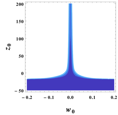
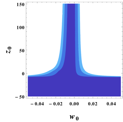
Let us consider an initial computation by assuming the best fit $\Omega_{m}^{0}=0.27$ for the $\Lambda$CDM model. Then, $\chi^{2}=\chi^{2}(w_{0},z_{0})$ and the results are shown in Table 1 and Fig. 6, where the $\chi_{min}^{2}$ value have a similar value in both parametrizations in comparison with the $\Lambda$CDM model and even lower for the parametrization $w_{1}$. the reduced $\chi^{2}$, defined as

$$\chi^{2}_{red}=\dfrac{\chi^{2}_{min}}{N_{data}-dof-1}$$ (32)

where $N_{data}$ is the number of experimental points used and the degree of freedom $dof$ is the number of parameters of the model, shows a better fit for the $\Lambda$CDM model. In both cases, $w_{0}=0$ corresponds to a cosmological constant, but does not coincide with the best fit, which is slightly displaced from that point whereas the $z_{0}$ parameter presents a large error since the second part of both parametrizations does not contribute when setting $w_{0}=0$. In both cases there are possibilities for the occurrence of a Big Rip singularity within the confidence region.

Table 1: Best fit for the models (20) and (21) with $\Omega_{0m}=0.27$ by using the Sne Ia dataset Suzuki:2011hu . The result for the $\Lambda$CDM model is also shown.

Model	$\bf{\chi_{min}^{2}}$	$\bf{w_{0}}$	$\bf{z_{0}}$	$\bf{\Omega_{0m}}$	$\bf{\chi_{red}^{2}}$
$\Lambda$CDM	$542.685$	-	-	$0.27\pm 0.02$	$0.978$
$w_{1}(z)$	$542.683$	$0.0045\pm 0.1$	$-25\pm 30$	$0.27$	$0.981$
$w_{2}(z)$	$541.583$	$-0.03\pm 0.07$	$22\pm 45$	$0.27$	$0.979$

(a)

(b)

Figure 6: Contour plots for the parameters $w_{0}$ and $z_{0}$ for the first (left) and second (right) models taking $\Omega_{0m}=0.27$.

(a)

(b)

Figure 7: Contour plots of the parameters $w_{0}$ and $z_{0}$ for $w_{1}$ (left) and $w_{2}$ (right) models using Standard Rulers data.

Figure 8: Contour plots for the first model (20) when using Sne Ia data and Standard Rulers.

Figure 9: Contour plots for the second model (21) when combining Sne Ia data and Standard Rulers.

Let us now use the Standard Ruler data to test the models (20) and (21). Standard Rulers are objects of known comoving size which may be used to measure the angular diameter distance. This data comes from two different sources: the Cosmic Microwave Background (CMB) Spergel:2006hy and the Baryon Acoustic Oscillations (BAO) Eisenstein:2005su .

In order to compute the theoretical points at early times it is necessary to consider the radiation contribution, $p_{rad}=\frac{1}{3}\rho_{rad}$, so that the FLRW equations (2) yield

$$H^{2}=\frac{\kappa^{2}}{3}\left(\rho_{m}+\rho_{rad}+\rho_{{}_{\phi}}\right)\ ,\quad\dot{H}=-\frac{\kappa^{2}}{2}\left[\rho_{m}+\frac{4}{3}\rho_{rad}+(1+w_{\phi})\rho_{{}_{\phi}}\right]\ .$$ (33)

By using the expressions of relative densities $\Omega_{i}^{0}=\rho_{0i}/\rho_{c}$, the FLRW equations (33) are describe as

$$E^{2}=\left[\Omega_{m}^{0}\ a^{-3}+\Omega_{rad}^{0}\ a^{-4}+\Omega_{\phi}^{0}X(a)\right]\$$ (34)

$$\dot{E}=-\frac{3}{2}\left[\Omega_{m}^{0}\ a^{-3}+\frac{4}{3}\Omega_{rad}^{0}\ a^{-4}+(1+w_{\phi})\Omega_{\phi}^{0}X(a)\right]\ ,$$ (35)

where $E=H/H_{0}$, $\Omega_{m}^{0}+\Omega_{rad}+\Omega_{\phi}=1$ for a flat universe and $X(a)$ is defined in terms of the scale factor as follows

$$X(a)={\rm exp}\left[-3\int_{1}^{a}\!\frac{(1+w(a^{\prime}))}{a^{\prime}}da^{\prime}\right]\ .$$ (36)

Since $\Omega_{m}^{0}$ and $\Omega_{rad}^{0}$ can be related, the above equations may be rewritten as follows

$$E^{2}(a)=\Omega_{m}(a+a_{eq})a^{-4}+\Omega_{de}{X(a)}$$ (37)

$$\dot{E}=-\frac{3}{2}\left[\Omega_{m}^{0}(a+\frac{4}{3}a_{eq})a^{-3}+(1+w_{DE})\Omega_{DE}^{0}X(a)\right]\ ,$$ (38)

where $a_{eq}=\Omega_{rad}/\Omega_{m}$, which can be expressed in terms of the redshift $a_{eq}=1/(1+z_{eq})$, where the equilibrium redshift is defined as the redshift when matter (baryons, electrons, and CDM) and radiation (photons and massless neutrinos) had the same density, $z_{eq}=2.5\times 10^{4}\Omega_{m}h^{2}(T_{CMB}/2.7\,{\rm K})^{-4}$, being $T_{CMB}$ the photon temperature of the CMB (see Eisenstein:1997ik ).

The $\chi^{2}_{CMB}$ is computed by using the dataset $(R,l_{a},\Omega_{b}h)$, Spergel:2006hy , where the first point is the scaled distance to recombination given by

$$R=\sqrt{\Omega_{0m}\frac{H_{0}^{2}}{c^{2}}}\;r(z_{CMB})\ ,$$ (39)

where $r(z_{CMB})$ is the comoving distance,

$$r(z)=\frac{c}{H_{0}}\int_{0}^{z}\frac{dz}{E(z)}\ .$$ (40)

The second point corresponds to the angular scale of the sound horizon at recombination,

$$l_{a}=\pi\frac{r_{(}a_{CMB})}{r_{s}(a_{CMB})}\ ,$$ (41)

where $a_{CMB}=\frac{1}{1+z_{CMB}}$ with $z_{CMB}=1089$ and being $r_{s}(a_{CMB})$ the comoving sound horizon at recombination,

$$r_{s}(a_{CMB})=\frac{c}{H_{0}}\int_{0}^{a_{CMB}}\frac{c_{s}(a)}{a^{2}E(a)}da\ ,$$ (42)

with the speed of sound $c_{s}(a)=1/\sqrt{3(1+\bar{R}_{b}a)}$, $\bar{R}_{b}=\frac{3}{4}\frac{\Omega_{b}h^{2}}{\Omega_{\gamma}h^{2}}=31500\Omega_{b}h^{2}(T_{CMB}/2.7K)^{-4}$ being the photon-baryon energy-density ratio and $\Omega_{b}$ the baryon density. The observational data is given by Spergel:2006hy

$$\bf{{\bar{V}}_{CMB}} = \left(\begin{array}[]{c}{\bar{R}}\\ {\bar{l}_{a}}\\ {\bar{\Omega}_{b}h}\end{array}\right)=\left(\begin{array}[]{c}1.70\pm 0.03\\ 302.2\pm 1.2\\ 0.022\pm 0.00082\end{array}\right)$$ (49)

Whereas the inverse covariance matrix is

$${\bf C_{CMB}}^{-1}=\left(\begin{array}[]{ccc}1131.32&4.8061&5234.42\\ 4.8061&1.1678&1077.22\\ 5234.42&1077.22&2.48145\times 10^{6}\end{array}\right).$$ (53)

Then, as usual the $\chi^{2}$ can be constructed by the difference between the experimental and theoretical points

$$\bf{X_{CMB}} = \left(\begin{array}[]{c}R-1.70\\ l_{a}-302.2\\ \Omega_{b}h^{2}-0.022\end{array}\right),$$ (57)

and the contribution to the $\chi^{2}$ by using the CMB dataset yields

$$\chi^{2}_{CMB}=\bf{X_{CMB}}^{T}{\bf C_{CMB}}^{-1}\bf{X_{CMB}}\ .$$ (58)

On the other hand, Table 2 contains the experimental points coming from the analysis of BAO, whereas the inverse covariant matrix is given by Eisenstein:2005su

$${\bf C_{BAO}}^{-1}=\left(\begin{array}[]{cccccc}4444.44&0&0&0&0&0\\ 0&30317&-17312&0&0&0\\ 0&-17312&87046&0&0&0\\ 0&0&0&1040.3&-807.5&336.8\\ 0&0&0&-807.5&3720.3&-1551.9\\ 0&0&0&336.8&-1551.9&2914.9\end{array}\right).$$ (65)

Table 2: Experimental BAO points: here $A(z)$ is the acoustic parameter and $d_{z}=r_{s}(z_{d})/D_{V}(z)$, being $D_{V}(z)$ is the dilation scale, Ref. Eisenstein:2005su . Points used for parameter fitting are bold font.

Sample		$\bf{z}$		$\bf{d_{z}}$		$\bf{A(z)}$
6dFGS		$0.106$		$\bf{0.336\pm 0.015}$		$0.526\pm 0.028$
SDSS		$0.2$		$\bf{0.1905\pm 0.0061}$		$0.488\pm 0.016$
SDSS		$0.35$		$\bf{0.1097\pm 0.0036}$		$0.484\pm 0.016$
WiggleZ		$0.44$		$0.0916\pm 0.0071$		$\bf{0.474\pm 0.034}$
WiggleZ		$0.6$		$0.0726\pm 0.0034$		$\bf{0.442\pm 0.020}$
WiggleZ		$0.73$		$0.0592\pm 0.0032$		$\bf{0.424\pm 0.021}$

Then, the contribution of BAO to the $\chi^{2}$ leads to

$$\chi^{2}_{BAO}=\bf{X_{BAO}}^{T}{\bf C_{BAO}}^{-1}\bf{X_{BAO}}\ ,$$ (66)

where $\bf{X_{BAO}}$ is the difference vector among the observational data in Table 2 and the theoretical points $\{d_{z}i$ and $A_{i}(z)\}$,

$${\bf{X_{BAO}}}^{\bf{T}}=\left(d_{z}1-0.336,\;d_{z}2-0.1905,\;d_{z}3-0.1097,\;A_{4}(z)-0.474,\;A_{5}(z)-0.442,\;A_{6}(z)-0.424\right)\ .$$ (67)

Hence, by minimizing $\chi^{2}=\chi_{CMB}^{2}+\chi_{BAO}^{2}$, the best fit for the above parametrizations is found. In the case of $\Lambda$CDM, the best fit leads to $\Omega_{0m}=0.249\pm 0.009$ and $\Omega_{b}=0.0428\pm 0.001$ which are then used for the calculation of $\chi^{2}$ for the models (20) and (21). The results are shown in Table 3 and Figure 7, where the best fit of the parameters $\{w_{0},z_{0}\}$ is quite close to the previous one obtained by using Sne Ia data, or at least within the confidence region. The large indetermination of the parameter $z_{0}$ is also appreciated because of the same point as above.

Table 3: Best fit for the models (20) and (21) by using BAO and CMB data, where $\Omega_{0m}=0.249$ and $\Omega_{b}=0.0428$ are assumed. The $\Lambda$CDM model gives $\chi^{2}_{min}=4.33$ and $\chi^{2}_{red}=0.619$.

Models		$\bf{\chi^{2}_{min}}$		$\bf{w_{0}}$		$\bf{z_{0}}$		$\chi^{2}_{red}$
$w_{1}$		$4.36$		$-0.09\pm 0.1$		$-18\pm 10$		$0.872$
$w_{2}$		$4.31$		$-0.009\pm 0.06$		$0.689654\pm 14$		$0.862$

Table 4: Best fit for the models (20) and (21) by combining Sne Ia data and standard rulers. The best fit for $\Lambda$CDM is also shown.

Model		$\bf{\chi^{2}_{min}}$		$\bf{\Omega_{0m}}$		$\bf{w_{0}}$		$\bf{z_{0}}$		$\chi^{2}_{red}$
$w_{1}$		$545.3$		$0.250\pm 0.002$		$-0.006\pm 0.03$		$8\pm 60$		$0.970$
$w_{2}$		$544.5$		$0.253\pm 0.005$		$-0.03\pm 0.02$		$40\pm 70$		$0.969$
$\Lambda$CDM		$548.1$		$0.250\pm 0.005$		$-$		$-$		$0.972$

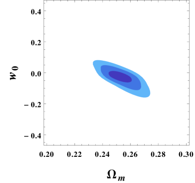
Finally, let us combine both datasets from previous analysis in order to get a better fit of the free parameters. The resulting grid of the free parameters $\chi(\Omega_{m}^{0},w_{0},z_{0})$, is analyzed where now $\Omega_{m}^{0}$ is kept as a free parameter. The results are shown in Table 4, where the best fit of the $\Lambda$CDM model is also included, whereas the resulting contour plots are depicted in Figs. 8-9. As shown, the best fit for the free parameters are within the confidence regions analyzed previously, whereas the reduced $\chi^{2}_{red}$ is smaller than the one obtained for the $\Lambda$CDM model. Nevertheless, the indetermination of the parameter $z_{0}$ remains very large as well as the error on the $w_{0}$ parameter in both models. In addition, the best fit for all the models gives a similar value for the relative matter density $\Omega_{m}^{0}\sim 0.25$, which state the high dependence of the cosmological evolution on matter density independently of the dark energy EoS.

V Discussions

In this paper, we have focused on the analysis of some parametrizations of the dark energy EoS, where we have implemented a new method to reconstruct a scalar field Lagrangian that gives rise to a particular EoS parameter. Parametrizing the dark energy EoS is commonly used to describe effectively the underlying theoretical model, since it facilitates the analysis of the dark energy EoS and its confrontation with the observational data. Within this aim we have focused on the reconstruction of a simple theoretical model, a (non)canonical scalar field, starting from the EoS parameter, where several examples have been studied. Then, two new parametrizations have been proposed, analyzed in terms of a scalar field and compared with the observational data. The aim of the proposed parametrizations has been to study the possibility of a fast transition and in particular the possibility of crossing the phantom barrier. Note that both models contain $\Lambda$CDM as a special case, when $w_{0}=0$, in which case the scalar field action reduces to a cosmological constant term, as shown in section II

Then, by using Supernova Ia and Standard Ruler data, both models have been analyzed and also compared with $\Lambda$CDM. The results show that both parametrizations leads to a $\chi^{2}_{min}$ value that is in general slightly smaller than the $\Lambda$CDM model whereas the value of the matter density yields $\Omega_{m}^{0}=0.25$ at the best fit. Besides, the resulting $\chi^{2}_{red}$ value within both models is below respect the resulting one for the $\Lambda$CDM model when using both standard candles as standard ruler data. In addition, the second parametrization (21) leads to better results regarding the value of the $\chi^{2}_{min\ (red)}$ in comparison with the parametrization (20).

Nevertheless, both parametrizations contain more free parameters than the $\Lambda$CDM model and specifically the parameter $z_{0}$ presents a large indetermination, specially when dealing with $z_{0}$ values that can not be constrained with experimental data. Furthermore, by analyzing the different approaches computed along the paper, the contour plots of both models show that $w_{0}\sim 0$ is very likely, in spite of the best fit is slightly displaced from $\Lambda$CDM. In addition, it is remarkable that both models do not lead to future singularities at the best fit, as shown in Table 4, and neither in most of the previous results, although the possibility of the occurrence of a future singularity is not excluded within the confidence region of the contour plots, as depicted in Figs. 6-9.

Indeed, while analyzing the first model with Sne Ia, the best fit yields $w_{0}$ very close to $0$ and Fig. 6 shows that a phantom transition is not excluded but unlikely. The fit with Standard Rulers leads to a similar result as well as when combining both datasets, as shown in Fig. 8, where specially the $w_{0}-\Omega_{m}^{0}$ contour plot favors $w_{0}\sim 0$. Nevertheless, the best fit for $w_{1}$ shows that the EoS parameter tends to an effective cosmological constant in the past ($z\gg 0$) whereas ends up slightly above the phantom barrier at small redshifts. Regarding the second parametrization (21), the $w_{0}$ parameter is always negative at the best fit independently of the data source used, which gives rise to an EoS parameter $w_{2}$ that crosses the phantom barrier at large redshifts $z\gg z_{0}$ for the best fit, whereas remains above the phantom barrier at small redshifts. In addition, $w_{0}\sim 0$ is also favored, as shown in the right panels of Figs. 6-7 and Fig. 9, but a phantom transition is within the confidence region of the contour plots, specifically the best fit leads to a phantom dark energy fluid in the past that tends to a non-phantom regime at small redshifts as pointed out above.

On the other hand, it is remarkable that neither models leads to future singularities at the best fit, as shown in Table 4, although the possibility of the occurrence of a future singularity is not excluded within the confidence region of the contour plots, as depicted in Figs. 6-9.

Hence, the analysis of the present manuscript shows that dealing with effective descriptions of the dark energy EoS can be well connected with the reconstruction of the underlying theory. In addition, both new parametrizations studied here show that a phantom epoch is compatible with the observational data in spite of that $\Lambda$CDM model is still very likely, although the best fit deviates a little bit from a cosmological constant. Moreover, the analysis shows that a singularity in the future is not excluded but also unlikely in both parametrizations.

Appendix

Here we reconstruct explicitly the scalar field Lagrangian by approximating the EoS’s (20) and (21) by Padé expansions, specifically the Padé approximation to the exponential function is used, which is given by

$$\exp(z)\approx\dfrac{p_{n}(z)}{p_{n}(-z)}\ ,$$ (68)

where

$$p_{n}(z)=\sum_{j=0}^{n}\frac{\binom{a}{b}}{j!\binom{a}{b}}z^{j}\;.$$ (69)

Then, the function $\tanh(z)=\dfrac{\exp(z)-\exp(-z)}{\exp(z)+\exp(-z)}$ can be expressed in terms of a Padé series as follows

$$\tanh(z)\approx F_{n}(z)=\frac{p_{n}(z)^{2}-p_{n}(-z)^{2}}{p_{n}(z)^{2}+p_{n}(-z)^{2}}\;.$$ (70)

In order to solve exactly the FLRW equation (8), which is not possible for the EoS’s (20) and (21), the above Padé approximation is assumed. The series (70) reproduces the behavior of (20) and (21) with a great accuracy, and in particular the fast transition that the EoS experiences. Hence, by assuming the $3^{rd}$ order of the Padé approximation (70),

$$\tanh(z-z_{0})\approx(z-z_{0})\frac{\left(z-z_{0}\right)^{2}+15}{6\left(z-z_{0}\right)^{2}+15}\;,$$ (71)

the scalar field Lagrangian can be reconstructed. Higher orders in (70) hold the same problem as the exact EoS, but third order is enough accurate. Hence, the Hubble parameter for the parametrization (20) by using the Padé approximation is given by

$$H(z)=A(z){\rm e}^{B(z)}\sqrt{C(z)}\ ,$$

where

$$A(z) = H_{0}\left(2z^{2}-4zz_{0}+2z_{0}^{2}+5\right)^{-\frac{25w_{0}(z_{0}+1)}{8\left(2z_{0}^{2}+4z_{0}+7\right)}}\ ,$$

$$B(z) = \frac{25w_{0}(z_{0}+1)\log\left[2(z-z_{0})^{2}+5\right]-4w_{0}\left\{z_{0}\left[z_{0}(z_{0}+9)+30\right]+37\right\}\log(z+1)}{8[2z_{0}(z_{0}+2)+7]}\ ,$$

$$C(z) = c_{1}\left[2(z-z_{0})^{2}+5\right]^{\frac{25w_{0}(z_{0}+1)}{4(2z_{0}(z_{0}+2)+7)}}\exp\left\{\frac{1}{4}w_{0}\left[\frac{25\sqrt{10}\tan^{-1}\left(\sqrt{\frac{2}{5}}(z-z_{0})\right)}{2z_{0}(z_{0}+2)+7}+2z+2\right]\right\}$$ (72)

$$+\Omega_{m}(z+1)^{\frac{w_{0}\{z_{0}[z_{0}(z_{0}+9)+30]+37\}}{2z_{0}(z_{0}+2)+7}+3}\ .$$

Note that the approximation (70) at third order fits the EoS (20) very accurately around the $z_{0}$, while far from this point, the deviation grows linearly by $\sim 6\%$ every $100z$. Nevertheless, the main feature of the above EoS (a fast transition at $z=z_{0}$) is greatly achieved by (70), while far away from $z_{0}$, the EoS (20) becomes constant (22). Then, the corresponding scalar field Lagrangian is reconstructed, where the kinetic term yields

$$\gamma(\phi)=\frac{c_{1}w_{0}}{\kappa^{2}\phi^{2}}\frac{a(\phi){\rm e}^{b(\phi)}}{c(\phi){\rm e}^{b(\phi)}+d(\phi)}\ ,$$

where

$$a(\phi) = \left\{-\left[z_{0}(z_{0}(z_{0}+9)+30)+37\right]\phi^{3}+3\left[z_{0}(z_{0}+6)+10\right]\phi^{2}-3(z_{0}+3)\phi+1\right\}$$

$$\times \left\{\frac{\left[2z_{0}(z_{0}+2)+7\right]\phi^{2}-4(z_{0}+1)\phi+2}{\phi^{2}}\right\}^{\frac{25w_{0}(z_{0}+1)}{4(2z_{0}(z_{0}+2)+7)}-1}\ ,$$

$$b(\phi) = \frac{1}{4}w_{0}\left\{\frac{2}{\phi}-\frac{25\sqrt{10}\tan^{-1}\left[\frac{\sqrt{\frac{2}{5}}(z_{0}\phi+\phi-1)}{\phi}\right]}{2z_{0}(z_{0}+2)+7}\right\}\ ,$$

$$c(\phi) = c_{1}\phi^{3}\left\{\frac{[2z_{0}(z_{0}+2)+7]\phi^{2}-4(z_{0}+1)\phi+2}{\phi^{2}}\right\}^{\frac{25w_{0}(z_{0}+1)}{4(2z_{0}(z_{0}+2)+7)}}\ ,$$

$$d(\phi) = \Omega_{m}\left(\frac{1}{\phi}\right)^{\frac{w_{0}\{z_{0}[z_{0}(z_{0}+9)+30]+37\}}{2z_{0}(z_{0}+2)+7}}\ .$$ (73)

While the potential scalar leads to

$$V(\phi)=-\frac{c_{1}H_{0}^{2}}{2\kappa^{2}}f(\phi){\rm e}^{j(\phi)}\ ,$$

where

$$f(\phi) = \left\{\phi^{3}\left[-(w_{0}(z_{0}(z_{0}(z_{0}+9)+30)+37)+6(2z_{0}(z_{0}+2)+7))\right]+3\phi^{2}(w_{0}(z_{0}(z_{0}+6)+10)+8(z_{0}+1))\right.$$

$$\left.-3\phi(w_{0}(z_{0}+3)+4)+w_{0}\right\}\times\left[\frac{2(z_{0}\phi+\phi-1)^{2}}{\phi^{2}}+5\right]^{\frac{25w_{0}(z_{0}+1)}{4(2z_{0}(z_{0}+2)+7)}-1}\left(\frac{1}{\phi}\right)^{3-\frac{w_{0}(z_{0}(z_{0}(z_{0}+9)+30)+37)}{2z_{0}(z_{0}+2)+7}}\ ,$$

$$j(\phi) = \frac{1}{4}w_{0}\left\{\frac{25\sqrt{10}\tan^{-1}\left[\sqrt{\frac{2}{5}}\left(-z_{0}+\frac{1}{\phi}-1\right)\right]}{2z_{0}(z_{0}+2)+7}+\frac{2}{\phi}\right\}\ .$$ (74)

In the same way, let us now consider the second parametrization (21). As above, by considering the Padé approximation at third order, the FLRW equation is solved exactly and the resulting Hubble parameter yields

$$H(z)=A(z)\exp^{B(z)}\sqrt{C(z)}\ ,$$

where,

$$A(z) = H_{0}\left(2z^{2}-4zz_{0}+2z_{0}^{2}+5\right)^{-\frac{25w_{0}(z_{0}+1)}{8\left(2z_{0}^{2}+4z_{0}+7\right)}}\ ,$$

$$B(z) = \frac{w_{0}(z_{0}+1)\left\{25\log\left[2(z-z_{0})^{2}+5\right]-4\left[z_{0}(z_{0}+2)+16\right]\log(z+1)\right\}}{8(2z_{0}(z_{0}+2)+7)}\ ,$$

$$C(z) = c_{1}\left[2(z-z_{0})^{2}+5\right]^{\frac{25w_{0}(z_{0}+1)}{4(2z_{0}(z_{0}+2)+7)}}\exp\left\{\frac{1}{4}w_{0}\left[\frac{25\sqrt{10}\tan^{-1}\left(\sqrt{\frac{2}{5}}(z-z_{0})\right)}{2z_{0}(z_{0}+2)+7}+2z+2\right]\right\}$$ (75)

$$+\Omega_{m}(z+1)^{\frac{w_{0}(z_{0}+1)[z_{0}(z_{0}+2)+16]}{2z_{0}(z_{0}+2)+7}+3}\ .$$

Then, the scalar Lagrangian for the parametrization $w_{2}$ can be reconstructed, where the kinetic term leads to

$$\gamma(\phi)=\frac{c_{1}w_{0}}{\kappa^{2}\phi^{2}}\frac{a(\phi){\rm e}^{b(\phi)}}{c_{1}\phi^{3}c(\phi){\rm e}^{b(\phi)}+d(\phi)}\ ,$$

where

$$a(\phi) = -(z_{0}\phi+\phi-1)\left\{[z_{0}(z_{0}+2)+16]\phi^{2}-2(z_{0}+1)\phi+1\right\}\left\{\frac{[2z_{0}(z_{0}+2)+7]\phi^{2}-4(z_{0}+1)\phi+2}{\phi^{2}}\right\}^{\frac{25w_{0}(z_{0}+1)}{4[2z_{0}(z_{0}+2)+7]}-1}\ ,$$

$$b(\phi) = \frac{1}{4}w_{0}\left\{\frac{2}{\phi}-\frac{25\sqrt{10}\tan^{-1}\left[\frac{\sqrt{\frac{2}{5}}(z_{0}\phi+\phi-1)}{\phi}\right]}{2z_{0}(z_{0}+2)+7}\right\}\ ,$$

$$c(\phi) = \left\{\frac{[2z_{0}(z_{0}+2)+7]\phi^{2}-4(z_{0}+1)\phi+2}{\phi^{2}}\right\}^{\frac{25w_{0}(z_{0}+1)}{4(2z_{0}(z_{0}+2)+7)}}\ ,$$

$$d(\phi) = \Omega_{m}\left(\frac{1}{\phi}\right)^{\frac{w_{0}(z_{0}+1)[z_{0}(z_{0}+2)+16]}{2z_{0}(z_{0}+2)+7}}\ .$$ (76)

And the scalar potential yields

$$V(\phi)=\frac{c_{1}H_{0}^{2}}{2\kappa^{2}}f(\phi){\rm e}^{j(\phi)}$$ (77)

where

$$f(\phi) = \left\{\left(-z_{0}+\frac{1}{\phi}-1\right)\left[w_{0}\left(\left(z_{0}-\frac{1}{\phi}+1\right)^{2}+15\right)+12\left(z_{0}-\frac{1}{\phi}+1\right)\right]-30\right\}\left[\frac{2(z_{0}\phi+\phi-1)^{2}}{\phi^{2}}+5\right]^{\frac{25w_{0}(z_{0}+1)}{4(2z_{0}(z_{0}+2)+7)}-1}$$

$$\times\left(\frac{1}{\phi}\right)^{-\frac{w_{0}(z_{0}+1)(z_{0}(z_{0}+2)+16)}{2z_{0}(z_{0}+2)+7}}\ ,$$

$$j(\phi) = \frac{1}{4}w_{0}\left\{\frac{25\sqrt{10}\tan^{-1}\left[\sqrt{\frac{2}{5}}\left(-z_{0}+\frac{1}{\phi}-1\right)\right]}{2z_{0}(z_{0}+2)+7}+\frac{2}{\phi}\right\}\ .$$ (78)

Hence, the parametrizations analyzed along this work can be constructed analytically in terms of the scalar field Lagrangian (1) by using Padé series.

References

• (1) S. Perlmutter et al. [SNCP Collaboration], Astrophys. J.  517, 565 (1999) [arXiv:astro-ph/9812133]; A. G. Riess et al. [Supernova Search Team Collaboration], Astron. J.  116, 1009 (1998) [arXiv:astro-ph/9805201].
• (2) D. N. Spergel et al. [WMAP Collaboration], Astrophys. J. Suppl.  148, 175 (2003) [arXiv:astro-ph/0302209]; E. Komatsu et al. [WMAP Collaboration], ibid180, 330 (2009) [arXiv:0803.0547 [astro-ph]]; ibid192, 18 (2011) [arXiv:1001.4538 [astro-ph.CO]];
• (3) D. N. Spergel et al. [WMAP Collaboration], Astrophys. J. Suppl.  170, 377 (2007) [astro-ph/0603449].
• (4) P. A. R. Ade et al. [Planck Collaboration], arXiv:1303.5076 [astro-ph.CO].
• (5) D. J. Eisenstein et al. [SDSS Collaboration], Astrophys. J.  633, 560 (2005) [arXiv:astro-ph/0501171]; W. J. Percival, S. Cole, D. J. Eisenstein, R. C. Nichol, J. A. Peacock, A. C. Pope and A. S. Szalay, Mon. Not. Roy. Astron. Soc.  381, 1053 (2007) [arXiv:0705.3323 [astro-ph]]. C. Blake, E. Kazin, F. Beutler, T. Davis, D. Parkinson, S. Brough, M. Colless and C. Contreras et al., Mon. Not. Roy. Astron. Soc.  418, 1707 (2011) [arXiv:1108.2635 [astro-ph.CO]].
• (6) Y. -F. Cai, E. N. Saridakis, M. R. Setare and J. -Q. Xia, Phys. Rept.  493, 1 (2010) [arXiv:0909.2776 [hep-th]]; K. Bamba, S. Capozziello, S. Nojiri and S. D. Odintsov, Astrophys. Space Sci.  342, 155 (2012) [arXiv:1205.3421 [gr-qc]]; E. J. Copeland, M. Sami and S. Tsujikawa, Int. J. Mod. Phys. D 15, 1753 (2006) [hep-th/0603057].
• (7) R.R. Caldwell, R. Dave, and P.J. Steinhardt, Phys. Rev. Lett. 80, 1582 (1998); E. Elizalde, S. Nojiri and S. D. Odintsov, Phys. Rev. D 70, 043539 (2004) [hep-th/0405034]. S. Capozziello, S. Nojiri, and S. D. Odintsov, Phys. Lett. B 632, 597 (2006) [arXiv:hep-th/0507182]; S. Nojiri and S. D. Odintsov, Gen. Rel. Grav. 38, 1285 (2006) [arXiv:hep-th/0506212]; S. Nojiri, S. D. Odintsov and H. Stefancic, Phys. Rev. D 74, 086009 (2006) [hep-th/0608168]; E. Elizalde, S. Nojiri, S. D. Odintsov, D. Saez-Gomez and V. Faraoni, Phys. Rev. D 77, 106005 (2008), [arXiv:0803.1311 [hep-th]]; S. Carloni, S. Capozziello, J. A. Leach and P. K. S. Dunsby, Class. Quant. Grav.  25, 035008 (2008) [gr-qc/0701009]. E. N. Saridakis and S. V. Sushkov, Phys. Rev. D 81, 083510 (2010) [arXiv:1002.3478 [gr-qc]]. T. Harko, F. S. N. Lobo and M. K. Mak, Eur. Phys. J. C 74, 2784 (2014) [arXiv:1310.7167 [gr-qc]];
• (8) L. H. Ford, Phys. Rev. D 40 (1989) 967. J. Beltrán Jiménez and A. L. Maroto, Phys. Rev. D 78 (2008) 063005; JCAP 0903 (2009) 016; Phys. Rev. D 80 (2009) 063512; T. Koivisto and D. F. Mota, JCAP 0808, 021 (2008); J. A. R. Cembranos, C. Hallabrin, A. L. Maroto, S. J. Nunez Jareno, Phys. Rev. D 86, 021301 (2012); arXiv:1212.3201 [astro-ph.CO].
• (9) S. Nojiri and S. D. Odintsov, eConf C0602061, 06 (2006) [Int. J. Geom. Meth. Mod. Phys. 4, 115-146 (2007)]; hep-th/0601213; arXiv: 0807.0685; Phys. Rept.  505, 59 (2011); Phys. Rev. D 68, 123512 (2003); [hep-th/0307288]; Phys. Lett. B 631 1 (2005); [arxiv:hep-th/0508049]; J. A. R. Cembranos, Phys. Rev.  D 73, 064029 (2006); Phys. Rev. Lett.  102, 141301 (2009); S. Capozziello and M. De Laurentis, Phys. Rept.  509, 167 (2011); S. Carloni, P. K. S. Dunsby, S. Capozziello and A. Troisi, Class. Quant. Grav.  22, 4839 (2005) [gr-qc/0410046]; S. Carloni, P. K. S. Dunsby and A. Troisi, Phys. Rev. D 77, 024024 (2008) [arXiv:0707.0106 [gr-qc]]; S. Nojiri, S. D. Odintsov and D. Sáez-Gómez, Phys. Lett. B 681, 74 (2009), arXiv:0908.1269 [hep-th]; A. de la Cruz-Dombriz and A. Dobado, Phys. Rev. D 74, 087501 (2006), gr-qc/0607118; T. P. Sotiriou and V. Faraoni, Rev. Mod. Phys.  82, 451 (2010); T. P. Sotiriou, J. Phys. Conf. Ser.  189, 012039 (2009); A. de la Cruz-Dombriz and D. Sáez-Gómez, Entropy 14, 1717 (2012), [arXiv:1207.2663 [gr-qc]]; F. D. Albareti et al., JCAP 1212, 020 (2012); arXiv:1212.4781 [gr-qc]. S. Capozziello and V. Faraoni, Beyond Einstein Gravity, Fundamental Theories of Physics Vol. 170, Springer Ed., Dordrecht (2011). S. Capozziello and M. Francaviglia, Gen. Rel. Grav.  40, 357 (2008), arXiv:0706.1146 [astro-ph]; G. Cognola, E. Elizade, S. Nojiri, S. D. Odintsov and S. Zerbini, Phys. Rev. D 73 084007 (2006), [arxiv:hep-th/0601008]; E. Elizalde, R. Myrzakulov, V. V. Obukhov and D. Sáez-Gómez, Class. Quant. Grav. 27 095007 (2010), [arXiv:1001.3636 [gr-qc]]; A. de la Cruz-Dombriz and D. Sáez-Gómez, Class. Quantum Grav. 29 245014, (2012), arXiv:1112.4481 [gr-qc].
• (10) S. Nojiri and S. D. Odintsov, Phys. Rev. D 72, 023003 (2005) [hep-th/0505215]; S. Capozziello, S. Nojiri and S. D. Odintsov, Phys. Lett. B 634, 93 (2006) [hep-th/0512118]; S. Capozziello, V. F. Cardone, E. Elizalde, S. Nojiri and S. D. Odintsov, Phys. Rev. D 73, 043512 (2006) [astro-ph/0508350]; D. F. Mota and C. van de Bruck, Astron. Astrophys.  421, 71 (2004) [astro-ph/0401504]; I. Brevik, O.G. Gorbunova and A. V. Timoshkin, Eur.Phys.J.C51:179-183,(2007) [arxiv:gr-qc/0702089] S. Nojiri and S. D. Odintsov, Phys. Lett. B 571, 1 (2003) [hep-th/0306212]; J. Sola and H. Stefancic, J. Phys. A 39, 6753 (2006) [gr-qc/0601012].
• (11) D. Huterer and M. S. Turner, Phys. Rev. D 64, 123527 (2001) [astro-ph/0012510]; J. Weller and A. Albrecht, Phys. Rev. D 65, 103512 (2002) [astro-ph/0106079].
• (12) D. A. Dicus and W. W. Repko, Phys. Rev.  D70 083527 (2004) [astro-ph/0407094].
• (13) M. Chevallier and D. Polarski, Int. J. Mod. Phys. D 10, 213 (2001) [gr-qc/0009008]; E. V. Linder, Phys. Rev. D 70, 023511 (2004) [astro-ph/0402503]; Rept. Prog. Phys.  71, 056901 (2008) [arXiv:0801.2968 [astro-ph]]; T. Padmanabhan and T. R. Choudhury, Mon. Not. Roy. Astron. Soc.  344, 823 (2003) [astro-ph/0212573].
• (14) R. Lazkoz, S. Nesseris and L. Perivolaropoulos, JCAP 0511, 010 (2005) [astro-ph/0503230].
• (15) R. Lazkoz, S. Nesseris and L. Perivolaropoulos, JCAP 0807, 012 (2008) [arXiv:0712.1232 [astro-ph]].
• (16) R. R. Caldwell, Phys. Lett. B 545 23 (2002), astro-ph/9908168; R. R. Caldwell, M. Kamionkowski and N. N. Weinberg, Phys. Rev. Lett. 91 071301 (2003), astro-ph/0302506; B. McInnes, JHEP 0208 029 (2002), hep-th/0112066; S. Nojiri and S. D. Odintsov, Phys. Lett. B 562 147 (2003), arXiv:hep-th/0303117; V. Faraoni, Int. J. Mod. Phys. D 11, 471 (2002), astro-ph/0110067; P. F. Gonzalez-Diaz, Phys. Lett. B 586 1 (2004), astro-ph/0312579; M. Sami and A. Toporensky, Mod. Phys. Lett. A 19 1509 (2004), gr-qc/0312009; H. Stefancic, Phys. Lett. B 586 5 (2004), astro-ph/0310904; M. P. Dabrowski, T. Stachowiak and M. Szydlowski, Phys. Rev. D 68, 103519 (2003) hep-th/0307128; L. P. Chimento and R. Lazkoz, Phys. Rev. Lett. 91 211301 (2003), gr-qc/0307111;Mod. Phys. Lett. A 19, 2479 (2004) [gr-qc/0405020]. F. S. N. Lobo, Phys. Rev. D 71, 084011 (2005) [gr-qc/0502099]. Yuri Shtanov, Varun Sahni, Class.Quant.Grav. 19 (2002) L101-L107, gr-qc/0204040; V. Sahni and Y. Shtanov, JCAP 0311, 014 (2003) [astro-ph/0202346]; A. V. Astashenok, S. Nojiri, S. D. Odintsov and A. V. Yurov, Phys. Lett. B 709 (2012) 396 [arXiv:1201.4056 [gr-qc]]; D. Sáez-Gómez, Phys. Rev. D 85, 023009 (2012), arXiv:1110.6033 [hep-th]; V. Sahni and Y. Shtanov, JCAP 0311, 014 (2003), astro-ph/0202346.
• (17) A. Vikman, Phys. Rev. D 71, 023515 (2005) [astro-ph/0407107];
• (18) S. Nojiri, S. D. Odintsov and S. Tsujikawa, Phys. Rev. D 71, 063004 (2005) [hep-th/0501025]. M. P. Dabrowski and T. Denkieiwcz, Phys. Rev. D 79, 063521 (2009) [arXiv:0902.3107 [gr-qc]]. M. P. Dabrowski and T. Denkiewicz, AIP Conf. Proc.  1241, 561 (2010) [arXiv:0910.0023 [gr-qc]].
• (19) J. D. Barrow, Class. Quant. Grav. 21, L79 (2004), gr-qc/0403084. J. D. Barrow, Class. Quant. Grav.  21, 5619 (2004), gr-qc/0409062;
• (20) J. D. Barrow, G. J. Galloway and F. J. Tipler Mon. Not. Roy. astr. Soc. 223, 835-844 (1986)
• (21) S. Nojiri and S. D. Odintsov, Phys. Rev. D 78, 046006 (2008), arXiv:0804.3519 [hep-th]; K. Bamba, C. Q. Geng, S. Nojiri and S. D. Odintsov, Mod. Phys. Lett. A 25, 900 (2010) arXiv:1003.0769 [hep-th]; K. Bamba, C. -Q. Geng, S. Nojiri and S. D. Odintsov, Phys. Rev. D 79, 083014 (2009) [arXiv:0810.4296 [hep-th]]; L. Fernandez-Jambrina and R. Lazkoz, Phys. Lett. B 670, 254 (2009), arXiv:0805.2284 [gr-qc]; K. Bamba, S. Nojiri and S. D. Odintsov, JCAP 0810, 045 (2008) [arXiv:0807.2575 [hep-th]]; K. Bamba, C. Q. Geng and C. C. Lee, JCAP 1011, 001 (2010) [arXiv:1007.0482 [astro-ph.CO]]; H. Motohashi, A. A. Starobinsky and J. ’i. Yokoyama, JCAP 1106 (2011) 006 [arXiv:1101.0744 [astro-ph.CO]]; D. Saez-Gomez, Class. Quant. Grav.  30, 095008 (2013) [arXiv:1207.5472 [gr-qc]].
• (22) R. Lazkoz, R. Maartens and E. Majerotto, Phys. Rev. D 74, 083510 (2006) [astro-ph/0605701]. S. Nesseris and L. Perivolaropoulos, JCAP 0701, 018 (2007) [astro-ph/0610092]. C. Kaeonikhom, B. Gumjudpai and E. N. Saridakis, Phys. Lett. B 695, 45 (2011) [arXiv:1008.2182 [astro-ph.CO]]. B. Novosyadlyj, O. Sergijenko, R. Durrer and V. Pelykh, Phys. Rev. D 86, 083008 (2012) [arXiv:1206.5194 [astro-ph.CO]]; JCAP  06 (2013) [arXiv:1212.5824 [astro-ph.CO]].
• (23) N. Suzuki, D. Rubin, C. Lidman, G. Aldering, R. Amanullah, K. Barbary, L. F. Barrientos and J. Botyanszki et al., Astrophys. J.  746, 85 (2012) [arXiv:1105.3470 [astro-ph.CO]].
• (24) P. H. Frampton, K. J. Ludwick and R. J. Scherrer, Phys. Rev. D 84, 063003 (2011), arXiv:1106.4996 [astro-ph.CO]; P. H. Frampton, K. J. Ludwick, S. Nojiri, S. D. Odintsov and R. J. Scherrer, Phys. Lett. B 708, 204 (2012), arXiv:1108.0067 [hep-th]. S. Nojiri, S. D. Odintsov and D. Sáez-Gómez, AIP Conf. Proc.  1458, 207 (2012), arXiv:1108.0767 [hep-th];
• (25) D. J. Eisenstein and W. Hu, Astrophys. J.  496, 605 (1998) [astro-ph/9709112].